Rational Jacobi Collocation Method for the Solution of the Boundary Layer Flow of an Eyring-Powell Non-Newtonian Fluid over a Linear Stretching Sheet

Abstract

In this paper, the Rational Jacobi (RJ) collocation method is proposed to approximate the solution of the boundary layer flow of an Eyring-Powell fluid over a stretching sheet. This equation is nonlinear and by applying Quasilinearization method (QLM), the equation is converted into a sequence of linear ordinary differential equations (ODE) converging to the solution of the nonlinear equation. Unlike other methods, instead of truncation in domain, the infinity condition is satisfied implicitly. As a result, using the proposed method, the model is converted to a system of linear algebraic equations. The effect of different parameters on the velocity profile is also presented.

1 Introduction

In engineering processes, It happened to have stretching surface with a velocity in an otherwise quiescent fluid. This stretching can cause a boundary layer viscous flow. This flow can be employed in metal extrusion, drawing of plastic films, polymer industry, glass blowing, paper production, wire drawing, extrusion of polymer, artificial fiber, spinning of filaments, hot rolling, crystal growing and so forth.

In order to make different sheets, the percentage of melting is crucial and to have a special thickness and other desired formats, we need to consider stretching and cooling rate in this process.

In 1970, Crane crane1970flow studied the flow of an incompressible viscous fluid pasting a stretching sheet.

Mukhopadhyay mukhopadhyay2013slip worked on the slip effects on Magnetohydrodynamic (MHD) boundary layer flow by an exponentially stretching sheet with suction/blowing and thermal radiation. Bhattacharyya bhattacharyya2012effects studied the effects of thermal radiation on micropolar fluid flow and heat transfer over a porous shrinking sheet.

Crane crane1970flow , Gupta gupta1977heat , Brady and Acrivos brady1981steady , Wang and Usha wang1990liquid , and Sridharan sridharan1995axisymmetric all investigated the Flow of Newtonian fluids.

Actually, Non-Newtonian fluids are more important than Newtonian fluids and their mathematical models are more complex than Newtonian fluids. The most frequent models that are used as Non-Newtonian models are power law, second grade, Maxwell and Oldroyd-B. Some uses of Non-Newtonian fluids are coal water, jellies, toothpaste, ketchup, food products, inks, glues, soaps and they are also used in polymer solutions hayat2013radiative . Unlike Newtonian fluids, mathematical systems for non-Newtonian fluids are of higher order and more difficult to deal with.

Nowadays, in addition to non-Newtonian, Eyring-Powell model is another model of interest. The Eyring-Powell model has advantages over the other non-Newtonian fluid models because instead of the empirical relation, it deduced from Kinetic theory of liquids. Another advantage of it is that it reduces to Newtonian behavior for low and high shear rates rahimi2016solution . In should be noted that in the calculation of fluid time scale at various polymer cases, Eyring-Powell fluid models are more accurate and consistent. Using Eyring-Powell model, Patel and Timol patel2009numerical , Hayat et al. hayat2012steady , Rosca and Pop rocsca2014flow and Jalil Jalil201373 investigated certain different facts and problems. Hayat et al hayaty also observed the unsteady flow of Eyring-Powell fluid past an inclined stretching sheet. They write that unsteadiness in the flow is due to the time-dependence of the stretching velocity and wall temperature and in their study the corresponding boundary layer equations are reduced into self-similar forms by suitable transformations then the analytic solutions are presented by homotopy analysis method (HAM). Furthermore, Sugunamma et al. sugu studied the effects of non uniform heat source/sink on unsteady flow of Powell-Eyring fluid past an inclined stretching sheet with suction/injection effects ,and the corresponding equations are transformed into a system of ordinary differential equations and solved it numerically using Runge- Kutta based shooting technique.

1.1 Problems defined on Unbounded Domain

To solve the problems that are defined on unbounded intervals, numerical or semi-analytical methods can be applied. Among semi-analytical methods, Adomian Decomposition tatari2007application , Homotopy Perturbation shakeri2008solution , Variational Iteration abdou2005variational and Exp-function MaW2010X methods can be pointed. Finite Difference dehghan2008 , Finite Element choi2016 , Meshfree Mirzaei2010 and Spectral methods parand2013 ; Rad2794 can be such categories of numerical methods.

1.2 Spectral Methods

In recent years, the study of Spectral methods for solving ODEs and partial differential equations (PDEs) has attracted much attentions. The reason why these methods are used substantially is the accuracy that these methods provide in solving linear and nonlinear phenomena like viscoelasticity, fluid mechanics, biology, physics and engineering. It is common to use orthogonal polynomials in the Spectral methods. There are so many authors being interested in utilizing these polynomials Bhrawyy2012 ; Doah2013 ; abd2013efficient ; doha2014chebyshev ; doha2015using . In recent years, in addition to the Spectral methods and orthogonal polynomials and functions, other methods have also been applied parand2013solving ; parandhemami ; ParandKHemamiM ; kazemRBF ; parand2016operation ; Rad2015363 ; Parand20144137 .
Generally, in simple geometries for smooth problems, the Spectral methods offer exponential rates of convergence/Spectral accuracy. Nevertheless, Finite Element and Finite Difference methods just propose algebraic convergence rates. Galerkin, Collocation and Tau methods are the three most widely used approaches in the Spectral methods.

To solve unbounded domain problems, several Spectral methods are used as different insights:

1) Direct approaches: In which orthogonal functions such as Sinc, Hermite, Bessel and Laguerre are used shen2000 ; GuoBY2007 ; Guo2003 ; MaH2007 . The main feature of these functions is that they are defined over the unbounded intervals.

2) Rational approximations: Where some Spectral methods on bounded domains are shifted into unbounded domains BoydJP1987 .

3) Mapping the problem of interest: By which the problem defined on an unbounded domain is mapped into a bounded domain problem GuoBY2010 .

4) Domain truncation: In this method, an enough large number is assumed to be on behalf of infinity in the domain and all the conditions for infinity should be satisfied by this large number BoydJP1988 .

1.3 Aim

Due to the accuracy needed to solve this problem defined on an unbounded domain, the presented method is introduced. In this method the domain is not truncated and the infinity condition is satisfied implicitly. To increase the numerical solution accuracy, Spectral collocation method based on orthogonal RJ functions are used and RJ basis are also formed. These basis are made just by using an algebraic mapping to change the standard Jacobi polynomials defined on $[-1,1]$ into the RJ functions on the domain $[0,\infty)$.

The rest of this paper is structured as follows. In the beginning, certain basic facts about the definition and description of the problem are reviewed, and the problem is formulated as a differential equation. Then, RJ collocation method is described and the approximation is introduced as if it satisfies the infinity condition. For linearizing the nonlinear problem of the sort, we applied the QLM to ease the calculation and make the equation more straightforward. In the end, we solved the problem and reported the results and conclusion.

2 Mathematical Formulation

In this section, over a linear stretching sheet one flow of a non-Newtonian Eyring-Powell fluid is investigated. The linear velocity of stretched sheet is shown as $\tau X$, where $\tau$=b is the linear stretching velocity and $X$ is the distance from the slit rahimi2016solution . In concise, we listed parameters to use them in the next formulations.

Table 1: Parameters and constants Description

Parameter(s)	Description	Parameter(s)	Description
$\xi_{ij}$ (kg/m $s^{2}$)	Shear-stress at the sheet	$\mu$ (kg/m s)	Dynamic viscosity of the fluid
$\gamma$	Material parameter	$H$	Material parameter
$u$, $v$ (m/s)	Non-dimensional velocity components along $X$- and $Y$-axes	$X$,$Y$ (m)	Non-dimensional Cartesian coordinates
$\kappa$ (m2/s)	Kinematic viscosity of the fluid	$\rho$(kg/m3)	Fluid density
$\tau$ (m/s)	Stretching velocity	$\phi$	Stream function
$f(x)$	Dimensionless stream function	$x$	Similarity variable
$\delta$	Non-dimensional fluid parameter	$\varepsilon$	Non-dimensional fluid parameter

As in rahimi2016solution mentioned, the extra stress tensor in an Eyring-Powell model is

$$\xi_{ij}=\mu\frac{\partial u_{i}}{\partial X_{j}}+\frac{1}{\gamma}sinh^{-1}\bigg{(}\frac{1}{H}\frac{\partial u_{i}}{\partial X_{j}}\bigg{)},$$

and considering

$$sinh^{-1}\bigg{(}\frac{1}{H}\frac{\partial u_{i}}{\partial X_{j}}\bigg{)}\cong\frac{1}{H}\frac{\partial u_{i}}{\partial X_{j}}-\frac{1}{6}\bigg{(}\frac{1}{H}\frac{\partial u_{i}}{\partial X_{j}}\bigg{)}^{3},\bigg{|}\frac{1}{H}\frac{\partial u_{i}}{\partial X_{j}}\bigg{|}<<1.$$

For the fluid based on Eyring-Powell model, the equation of continuity and the $X$-momentum equation is simplified as

$$\frac{\partial u}{\partial X}+\frac{\partial v}{\partial Y}=0,$$

$$u\frac{\partial u}{\partial X}+v\frac{\partial v}{\partial Y}=\frac{\partial^{2}u}{\partial Y^{2}}\bigg{(}\kappa+\frac{1}{\rho\gamma H}\bigg{)}-\frac{1}{2\rho\gamma H^{3}}\bigg{(}\frac{\partial u}{\partial Y}\bigg{)}^{2}\frac{\partial^{2}u}{\partial Y^{2}},$$ (1)

and the boundary conditions are

$$u=\begin{cases}bX,&Y=0,\\ 0,&Y\rightarrow\infty,\\ \end{cases}$$

additionally, if we set

$$u=\frac{\partial\phi}{\partial Y},v=-\frac{\partial\phi}{\partial X},$$

$$\phi=Xf(x)(b\kappa)^{0.5},x=Y(\frac{b}{\kappa})^{0.5}.$$ (2)

where $x$ is the similarity variable. Consequently, Eq.(1) and Eq.(2) lead to

$$f(x)f^{\prime\prime}(x)+(1+\varepsilon)f^{\prime\prime\prime}(x)-\varepsilon\delta f^{\prime\prime}(x)^{2}f^{\prime\prime\prime}(x)-f^{\prime}(x)^{2}=0,$$ (3)

and boundary conditions will be enhanced as $f(0)=0$ and

$$f^{\prime}(x)=\begin{cases}1,&x\rightarrow 0,\\ 0,&x\rightarrow\infty.\\ \end{cases}$$

The constant parameters $\delta$, $\varepsilon$ are the Non-dimensional fluid parameter which are considered constant in numerical examples. In fact, these quantities have the following definitions rahimi2016solution

$$\varepsilon=\frac{1}{\mu\gamma H},\leavevmode\nobreak\ \leavevmode\nobreak\ \delta=\frac{b^{3}X^{2}}{2H^{2}\kappa}.$$ (4)

3 Preliminaries

3.1 Jacobi Polynomials

Because of the features that Jacobi polynomials provide, these polynomials are considered to solve different types of problems ParandLatifi ; bhrawyzaky2015 ; bhrawyAlzaidy ; BhrawyDoha2015 ; BhrawyAHDohaEH2015 ; Doha2015pseudo . The standard Jacobi polynomial of degree $n$ with $\alpha,\beta>-1$ is as follows shen2011spectral

$$J_{n}^{\alpha,\beta}(x)=\bigg{(}\frac{\Gamma(n+\alpha+1)}{n!\Gamma(n+\alpha+\beta+1)}\bigg{)}\sum_{i=0}^{n}\binom{n}{i}\frac{\Gamma(n+i+\alpha+\beta+1)}{\Gamma(i+\alpha+1)}{\frac{(x-1)}{2}}^{i},$$

with the properties as:

$$J_{n}^{\alpha,\beta}(-x)=(-1)^{n}J_{n}^{\beta,\alpha}(x),J_{n}^{\alpha,\beta}(-1)=\frac{(-1)^{n}\Gamma(n+\beta+1)}{n!\Gamma(\beta+1)},J_{n}^{\alpha,\beta}(1)=\frac{\Gamma(n+\alpha+1)}{n!\Gamma(\alpha+1)}.$$

and its weight function is $w^{\alpha,\beta}(x)=(1-x)^{\alpha}(1+x)^{\beta}$.
These polynomials are orthogonal on $[-1,1]$

$$\int_{-1}^{1}{J_{n}^{\alpha,\beta}(x)J_{m}^{\alpha,\beta}(x)}w^{\alpha,\beta}(x)=\delta_{m,n}\frac{2^{\alpha+\beta+1}\Gamma(n+\alpha+1)\Gamma(n+\beta+1)}{(2n+\alpha+\beta+1)\Gamma(n+1)\Gamma(n+\alpha+\beta+1)},$$

where $\delta_{m,n}$ is

$$\delta_{m,n}=\begin{cases}1,&m=n,\\ 0,&m\neq n.\\ \end{cases}$$

The set of Jacobi polynomials makes a complete $L_{w^{\alpha,\beta}}^{2}[-1,1]$ orthogonal system.

3.2 Rational Jacobi (RJ) Functions

In spite of $[-1,1]$, the equation of interest is defined over an unbounded domain; To have all the properties of Jacobi polynomials on unbounded domain, we can use the mapping $\frac{x-L}{x+L}$ ParandKMazaherithomas . Using this mapping will lead to creation of RJ Basis defined as

$$RJ_{n,L}^{\alpha,\beta}(x)=J_{n}^{\alpha,\beta}(\frac{x-L}{x+L}).$$

These new RJ functions, inherit most of the useful characteristics of the standard Jacobi polynomials. Of these characteristics can mention: simplicity, exponential or infinite order convergence, completeness and having real roots that are spread on $[0,\infty)$. By this, the domain will be $[0,\infty)$. Putting this mapping relation in standard Jacobi polynomials formula, we have

$$RJ_{n,L}^{\alpha,\beta}(x)=\bigg{(}\frac{\Gamma(n+\alpha+1)}{n!\Gamma(n+\alpha+\beta+1)}\bigg{)}\sum_{i=0}^{n}\binom{n}{i}\frac{\Gamma(n+i+\alpha+\beta+1)}{2\Gamma(i+\alpha+1)}{{\bigg{(}(\frac{x-L}{x+L})-1\bigg{)}}}^{i},$$

and

$$RJ_{n,L}^{\alpha,\beta}(-x)=(-1)^{n}RJ_{n,L}^{\beta,\alpha}(x),RJ_{n,L}^{\alpha,\beta}(0)=\frac{(-1)^{n}\Gamma(n+\beta+1)}{n!\Gamma(\beta+1)},RJ_{n,L}^{\alpha,\beta}(\infty)=\frac{\Gamma(n+\alpha+1)}{n!\Gamma(\alpha+1)}.$$

The above mentioned weight function for these new rational functions is $w_{L}^{\alpha,\beta}(x)=(1-(\frac{x-L}{x+L}))^{\alpha}(1+(\frac{x-L}{x+L}))^{\beta}\frac{2L}{(x+L)^{2}}$. This weight function can be simplified to the form

$$w_{L}^{\alpha,\beta}(x)=\frac{2^{\alpha+\beta+1}x^{\beta}L^{\alpha+1}}{(x+L)^{\alpha+\beta+2}}.$$

Obviously, this weight function is non-negative, integrable and in fact, that is a real-valued weight function over $[0,\infty)$.
Moreover, RJ functions are orthogonal on $[0,\infty)$

$$\int_{0}^{\infty}{RJ_{n,L}^{\alpha,\beta}(x)RJ_{m,L}^{\alpha,\beta}(x)}w_{L}^{\alpha,\beta}(x)=\delta_{m,n}\frac{2^{\alpha+\beta+1}\Gamma(n+\alpha+1)\Gamma(n+\beta+1)}{(2n+\alpha+\beta+1)\Gamma(n+1)\Gamma(n+\alpha+\beta+1)}.$$

The set of RJ functions makes a complete $L_{w_{L}^{\alpha,\beta}}^{2}[0,\infty)$ orthogonal system and for any $y(x)\in L_{w_{L}^{\alpha,\beta}}^{2}[0,\infty),$ there is an expansion as follows.

$$y(x)=\sum_{j=0}^{\infty}b_{j}RJ_{j,L}^{\alpha,\beta}(x).$$

4 Quasilinearization Method (QLM)

In reality, many of equations are nonlinear and difficult to deal with. One way to make these equations linear and utilize their linearity property is to use QLM. QLM is based on Newton-Raphson method khan2006generalized ; el2006generalized ; vatsala1999generalized ; el2007quasilinearization by which in an iterative view, we suppose that the solution of $i^{th}$ step is known and we attempt to find the solution in $(i+1)^{th}$ step. Although it is an iterative method, the QLM is not perturbative and the fast quadratic convergence is the most dominant quality of it MandelzweigVB .

This method was developed by Bellman and Kalaba KalabaR ; BellmanRE and can be applied to solve miscellaneous nonlinear ODEs or partial differential equations (PDEs) in such different fields of sciences like physics, engineering and biology. As a matter of fact, by using QLM, a nonlinear equation can be converted into a linear equation in which the solution converges to the solution of the nonlinear equation. It is worth mentioning that in delkhoshtomas , the convergence of QLM has been discussed and proved. The QLM iteration requires an initialization or ”initial guess” that is chosen from physical and mathematical considerations or the boundary conditions in the equation.

To know how it works, imagine that we have one particular differential equation as:

$$L^{(m)}(y(x))=h(x,y(x),y^{(1)}(x),y^{(2)}(x),...,y^{(m-1)}(x)).$$

where $L^{(m)}$ is the differential operator of order $m$, and $h(x,y(x),y^{(1)}(x),y^{(2)}(x),...,y^{(m-1)}(x))$ is a nonlinear function containing $x,y(x),y^{\prime}(x),...,y^{(m-1)}(x)$ .
The linear equation after applying QLM will be

$$L^{(m)}(y_{i+1}(x))=h\big{(}x,y_{i}(x),y_{i}^{(1)}(x),y_{i}^{(2)}(x),...,y_{i}^{(m-1)}(x)\big{)}+$$

$$\sum_{j=0}^{m-1}{\big{(}y_{i+1}^{(j)}(x)-y_{i}^{(j)}(x)\big{)}h_{y^{(j)}}\big{(}x,y_{i}(x),y_{i}^{(1)}(x),y_{i}^{(2)}(x),...,y_{i}^{(m-1)}(x)\big{)}.}$$

Convergence of the QLM proved by Bellman & Kalaba BellmanRE and Mandelzweig & Tabakin mandelzweig2001quasilinearization .
If $\delta y_{i+1}(x)\equiv y_{i+1}(x)-y_{i}(x)$ be the difference between two subsequent iterations, then, $\|\delta y{i+1}\|\leq k\|\delta y_{i}\|^{2}$, where k is a real constant. Therefore the convergence rate is of order 2 i.e. $O(h^{2})$. It worth mentioning that the order of convergence in numerical methods can be affected and reduced by the errors in computational methods, machine errors, roundoff errors, and so forth.
Additionally we have the relationship

$$\|\delta y_{i+1}\|\leq(\|\delta y_{1}\|)^{(2^{n})}/k$$

and we can say that the convergence depends on $q_{1}=k\|\delta y_{1}\|=k\|\delta y_{1}-y_{0}\|$. For convergence it is sufficient that just one of $q_{m}=k\|\delta y_{m}\|$ be small enough. Even if the first convergent coefficient $q_{1}$ is large, a well chosen value for $y_{0}$ results in a small value for at least one of $q_{m},m\geq 2$ and this also reduces the order of convergence. BellmanRE ; mandelzweig2001quasilinearization .

Considering Eq.(3), the Eyring-Powell equation of interest is linearized and Eq.(5) is achieved. For the purpose of simplicity [(.) $\equiv$ $\big{(}x,f_{i}(x),f^{\prime}_{i}(x),f^{\prime\prime}_{i}(x)\big{)}$] is assumed (See Appendix).

$$g_{1}(.)+g_{2}(.)f_{i+1}(x)+g_{3}(.)f^{\prime}_{i+1}(x)+g_{4}(.)f^{\prime\prime}_{i+1}(x)-f^{\prime\prime\prime}_{i+1}(x)=0,$$ (5)

where $g_{j}(.),j=1,2,3,4$ are all known and $f_{i+1}(x)$ is unknown and at the initial step $f_{0}:=1$. Clearly, the Eq.(5) is linear. From now on, instead of the former nonlinear equation, this linear equation is under consideration and in the next sections we attempt to solve it numerically.

5 Rational Jacobi (RJ) Collocation Method

In collocation method, It matters that how collocation points are chosen. Choosing these points can even affect convergence and efficiency. Here in this paper, we approximate the solution in an expansion like Eq.(6). If $y(x)$ be the solution of our ODE, by continuing in $N+1$ points, its approximated expansion in iteration $(i+1)^{th}$ i.e. $f_{i+1}(x)$ will be

$$y(x)\cong f_{i+1}(x)=\frac{x}{x^{2}+1}+\frac{x^{2}}{x^{2}+1}\sum_{j=0}^{N}{a_{j}^{i+1}RJ_{j,L}^{\alpha,\beta}(x)},$$ (6)

in which all the following conditions are satisfied.

$$\lim_{x\to 0}f_{i+1}(x)=0,\lim_{x\to 0}f_{i+1}^{\prime}(x)=1,\lim_{x\to\infty}f_{i+1}^{\prime}(x)=0.$$

Considering Eq.(5) we can show the residual function as (in order to read more on this residual function see Appendix)

$$Res(x;a_{0}^{i+1},a_{1}^{i+1},...,a_{N}^{i+1})=-f^{\prime\prime\prime}_{i+1}(x)+g_{1}(.)+g_{2}(.)f_{i+1}(x)+g_{3}(.)f^{\prime}_{i+1}(x)+g_{4}(.)f^{\prime\prime}_{i+1}(x),$$

In which, $g_{k}(.),k=1,2,3,4$ are known (defined in Appendix) and the $f_{i+1}(x)$ is unknown and we are to approximate it. To find the unknown $a_{j}^{i+1},j=0,..,N$ we appoint the RJ collocation points($x_{k}$, $k=0,...,N$) and solve the system in Eq.(7). These collocation points are the roots of $RJ_{N+1,L}^{\alpha,\beta}(x)$.

$$Res(x_{k};a_{0}^{i+1},a_{1}^{i+1},...,a_{N}^{i+1})=0,k=0,...,N.$$ (7)

6 Numerical Results

After solving the system of equations mentioned in Eq.(7) we listed the values of resulted solutions. In Table(2) the result of $f(x)$,$f^{\prime}(x)$ and $f^{\prime\prime}(x)$ for different $N$(Collocation points) are reported.
As discussed earlier, the presented error is implemented without truncating domain. In order to show the accuracy of the presented mthod in Table (3) we made a comparison with other methods: IRBFs-QLM method lotfibaba ; Rational Chebyshev collocation method with truncation in domain parandmoayeri ; Runge-Kutta method; Collocation method with basis functions $\{1,x,x^{2},...\}$ and truncation in domain lotfibaba . From this table can draw a conclusion that since the Runge-Kutta 4th order method is exact at least up to 4 digitslotfibaba , the presented method with no truncation is more accurate than Rational Chebychev collocation method endowed with truncation in domain. This is also more accurate than CM (collocation method with basis functions $\{1,x,x^{2},...\}$).
In Fig.(1(a),1(b),1(c) and 1(d)) and fig.(2(a),2(b),2(c) and 2(d)) we showed that as the steps of iteration in QLM or Collocation points ($N$) increases the obtained result is better, the diagrams are smoother and the Logarithm of the absolute residual is closer to zero.
In Fig.(3(a)) and fig.(3(b)) the effects of the non-Newtonian fluid parameters i.e $\delta$ and $\varepsilon$ on the non-dimensional velocity and stress field ($f^{\prime}(x)$ and $f^{\prime\prime}(x)$) are presented. It is concluded that when $\varepsilon$ increases or $\delta$ decreases, $f^{\prime}(x)$ increases. if $\delta$ increases or $\varepsilon$ decreases, as a result $f^{\prime\prime}(x)$ will increase.
If the obtained solution ($f_{i+1}(x)$) is put in the original equation (Eq. (3)), the residual function will be defined as

$$res(x)=f_{i+1}(x)f_{i+1}^{\prime\prime}(x)+(1+\varepsilon)f_{i+1}^{\prime\prime\prime}(x)-\varepsilon\delta f_{i+1}^{\prime\prime}(x)^{2}f_{i+1}^{\prime\prime\prime}(x)-f_{i+1}^{\prime}(x)^{2},$$ (8)

The correctness and convergence of the method is illustrated by plotting residual function ($res(x)$) and the values of coefficients existed in Eq.(6) are also denoted. To calculate an approximation of the optimal value of parameter L we used the following fact:
”The experimental trial-and-error method(Optimizing Infinite Interval Map Parameter) boyd2001 : Plot the coefficients $a_{j}$ versus degree on a log-linear plot. If the graph abruptly flattens at some $N$, then this implies that $L$ is TOO SMALL for the given $N$, and one should increase $L$ until the flattening is postponed to $j=N$.”

Based on this fact, the optimal parameter L is shown in Fig. 6. This optimal value is seemed to be $L=15$. Additionally, because the diagram of the coefficient $a_{j},j=0,...,N$ decreases, it is obvious that the presented method is convergent.

Table 2: The numerical results in the 15th iteration for $f$,$f^{\prime}$,$f^{\prime\prime}$ for different $N$. $\delta=0.1$, $\varepsilon=0.3$, $\alpha=1,\beta=1$, $L=15$.

	x	N=10	N=15	N=25	N=50
f	0.0	0.0000000000	0.0000000000	0.0000000000	0.0000000000
	0.5	0.4036738856	0.4045266250	0.4045235026	0.4045235024
	1	0.6658626593	0.6652631608	0.6652578446	0.6652578448
	1.5	0.8353708975	0.8334184925	0.8334154070	0.8334154068
	2.0	0.9443573988	0.9418982540	0.9418951684	0.9418951684
	2.5	1.0144374602	1.0118879495	1.0118841902	1.0118841903
	3.0	1.0595784826	1.0570456452	1.0570418968	1.0570418967
	3.5	1.0887030794	1.0861819735	1.0861787456	1.0861787455
	4.0	1.1075132470	1.1049814404	1.1049787070	1.1049787070
	4.5	1.1196651637	1.1171115798	1.1171090443	1.1171090444
	5.0	1.1275118485	1.1249385493	1.1249359382	1.1249359382
f’	0.0	1.0000000000	1.0000000000	1.0000000000	1.0000000000
	0.5	0.6450803420	0.6442642937	0.6442495479	0.6442495461
	1.0	0.4189562550	0.4154133505	0.4154176707	0.4154176711
	1.5	0.2697139887	0.2679636516	0.2679659918	0.2679659914
	2.0	0.1733336877	0.1728814969	0.1728800369	0.1728800375
	2.5	0.1115538147	0.1115431922	0.1115424083	0.1115424080
	3.0	0.0719247489	0.0719686778	0.0719693974	0.0719693972
	3.5	0.0464362346	0.0464355030	0.0464366676	0.0464366678
	4.0	0.0299991498	0.0299616664	0.0299623908	0.0299623909
	4.5	0.0193776822	0.0193326322	0.0193327138	0.0193327137
	5.0	0.0125058088	0.0124744388	0.0124741099	0.0124741098
f”	0.0	-0.9192031329	-0.8809437796	-0.8807848835	-0.8807849724
	0.5	-0.5513725007	-0.5658276136	-0.5658037464	-0.5658037300
	1.0	-0.3662977979	-0.3643882166	-0.3643723455	-0.3643723552
	1.5	-0.2385329622	-0.2348981506	-0.2349101459	-0.2349101417
	2.5	-0.0981133286	-0.0977533531	-0.0977500466	-0.0977500475
	3.0	-0.0630210169	-0.0630697634	-0.0630676466	-0.0630676457
	3.5	-0.0405944573	-0.0406920734	-0.0406922931	-0.0406922928
	4.0	-0.0262103556	-0.0262544563	-0.0262557467	-0.0262557472
	4.5	-0.0169503305	-0.0169398783	-0.0169410136	-0.0169410139
	5.0	-0.0109702242	-0.0109304115	-0.0109308917	-0.0109308915

Table 3: The value of $f^{\prime}$ by presented method and other methods in the 15th iteration. $N=10$, $\delta=0.1$, $\varepsilon=0.3$, $\alpha=1,\beta=1$ and $L=15$.

x	CM lotfibaba	Runge-katta lotfibaba	IRBFs-QLM lotfibaba	Rational Chebyshev parandmoayeri	Presented method
0	0.99999	1	1	1	1
1	0.41411	0.41542	0.41542	0.4158220240	0.4189562550
2	0.16994	0.17288	0.17288	0.1737538392	0.1733336877
3	0.06748	0.07197	0.07197	0.0732981252	0.0719247489
4	0.02426	0.02996	0.02996	0.0316552721	0.0299991498
5	0.00593	0.01247	0.01247	0.0144254667	0.0125058088

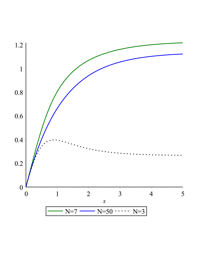
(a) $f(x)$

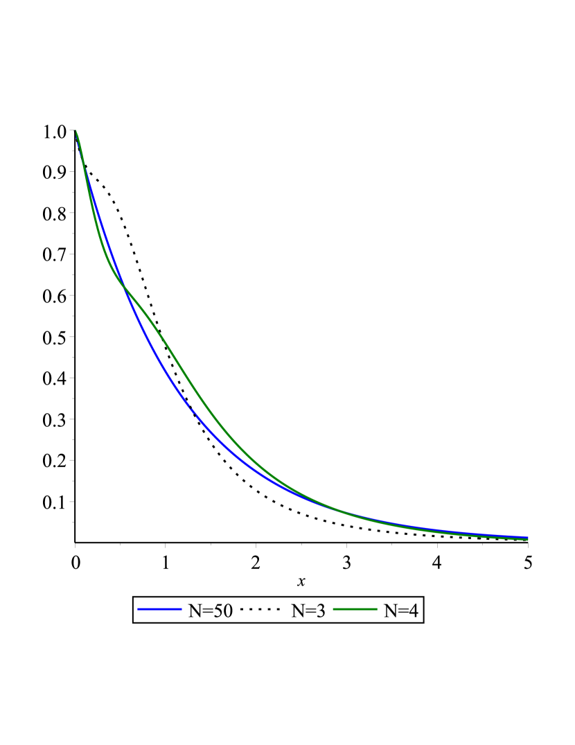
(b) $f^{\prime}(x)$

(c) $f^{\prime\prime}(x)$

(d) Logarithm of the absolute value of residual.

Figure 1: Diagram of $f(x)$, $f^{\prime}(x)$, $f^{\prime\prime}(x)$ and $Log(|res(x)|)$ in the $25$th iteration for different $N$. $\delta=0.1$, $\varepsilon=0.3$, $\alpha=1,\beta=1$, $L=15$.

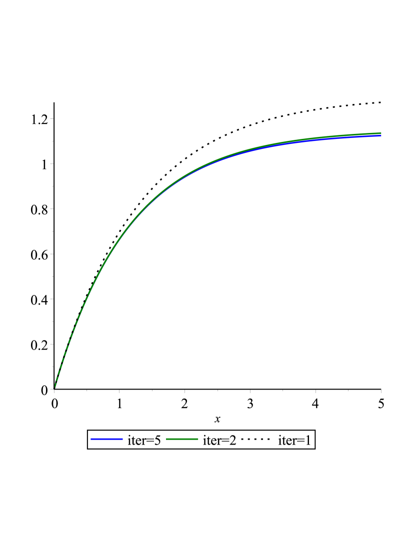
(a) $f(x)$

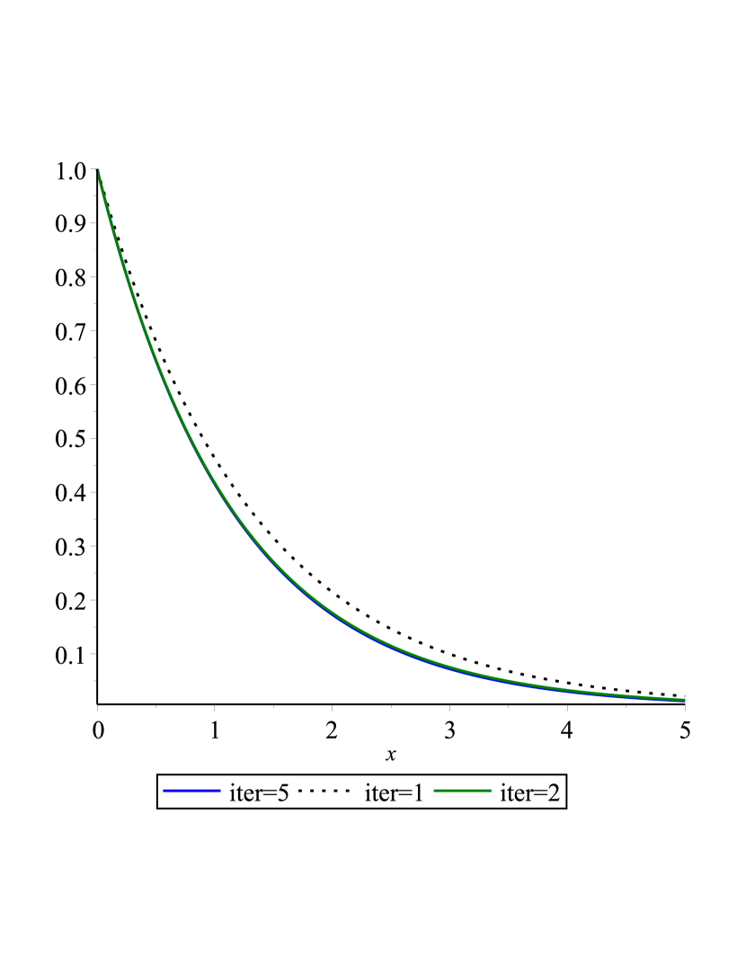
(b) $f^{\prime}(x)$

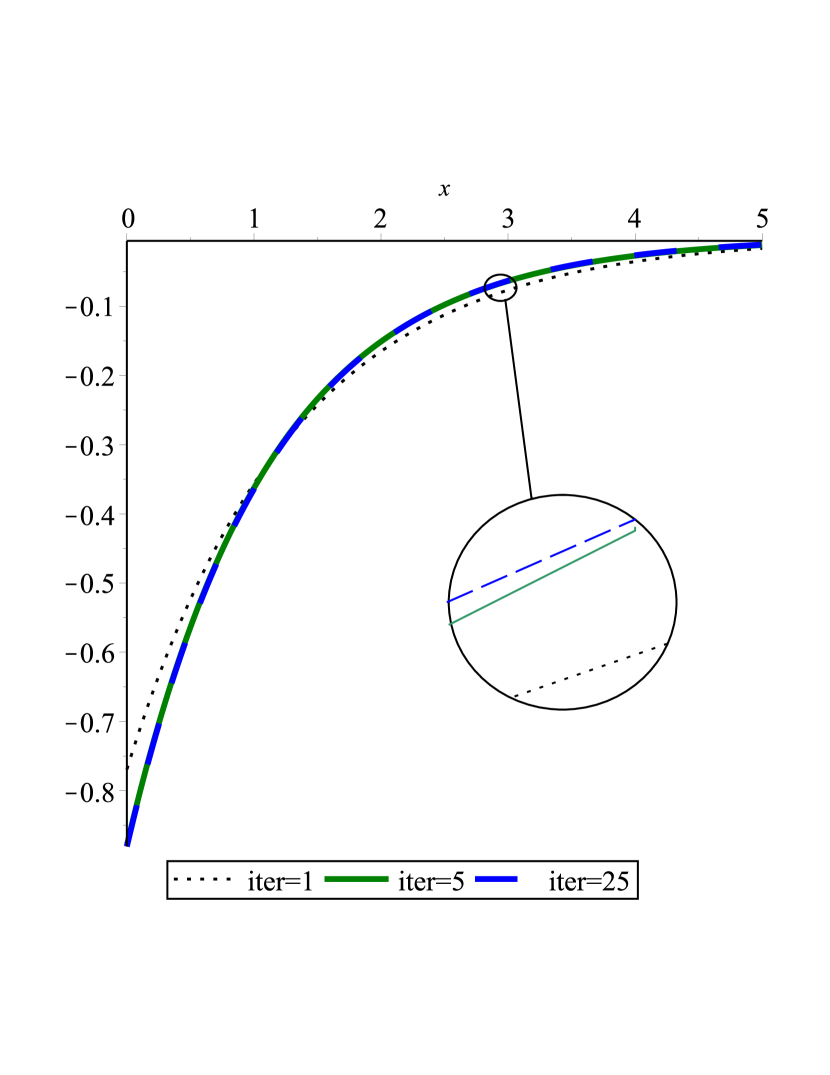
(c) $f^{\prime\prime}(x)$

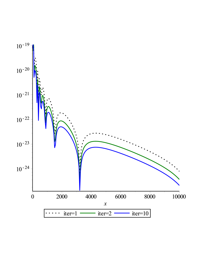
(d) Logarithm of the absolute value of residual.

Figure 2: Diagram of $f(x)$, $f^{\prime}(x)$, $f^{\prime\prime}(x)$ and $Log(|Res(x)|)$ for $N=50$ in different iterations. $\delta=0.1$, $\varepsilon=0.3$, $\alpha=1,\beta=1$, $L=15$.

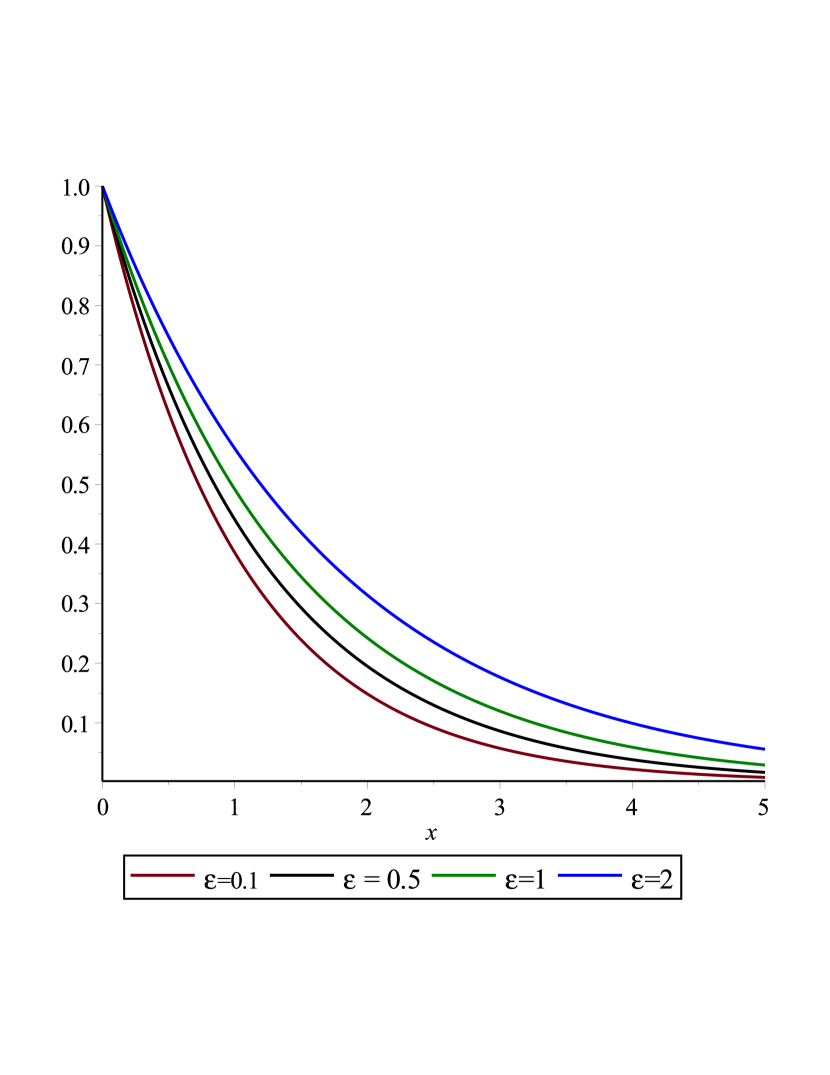
(a) $f^{\prime}(x)$

(b) $f^{\prime\prime}(x)$

Figure 3: Diagram of the effect of $\varepsilon$ on $f^{\prime}(x)$ and $f^{\prime\prime}(x)$ in $15$th iteration. $\delta=0.2$, $N=50$, $\delta=0.2$ ,$\alpha=1,\beta=1$, $L=15$.

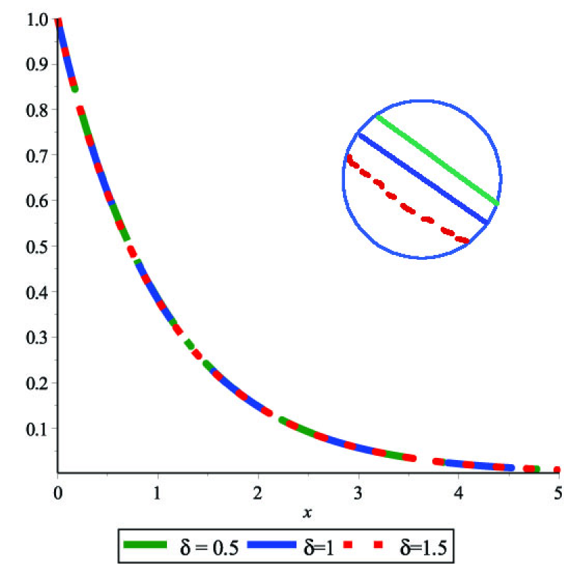
(a) $f^{\prime}(x)$

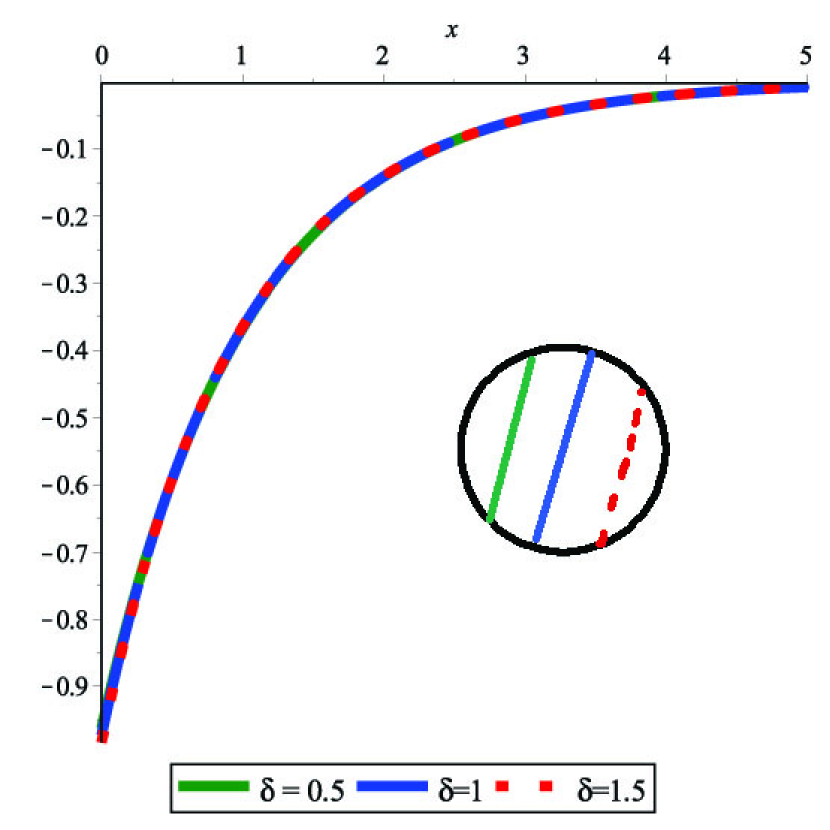
(b) $f^{\prime\prime}(x)$

Figure 4: Diagram of the effect of $\delta$ on $f^{\prime}(x)$ and $f^{\prime\prime}(x)$ in the $15$th iteration. $N=50$, $\varepsilon=0.1$ ,$\alpha=1,\beta=1$, $L=15$.

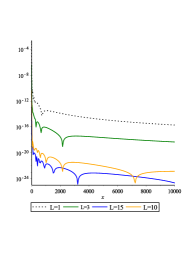
Figure 5: Logarithm of the absolute value of residual in the $15$th iteration by different $L$. $N=50$, $\varepsilon=0.3$, $\delta=0.1$, $\alpha=1,\beta=1$.

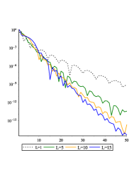
Figure 6: Logarithm of the absolute value of coefficients $\big{(}Log(|a_{j}^{i+1}|),j=0,...,N\big{)}$ that show the optimal value of $L$ in the $25$th iteration. $N=50$, $\varepsilon=0.3$, $\delta=0.1$, $\alpha=1,\beta=1$.

7 conclusion

In this paper, the RJ collocation method applied for a nonlinear equation of momentum with an infinite condition and the velocity and stress profiles of a non-Newtonian Eyring-Powell fluid over a linear stretching sheet is studied. Due to encountering with an unbounded domain, we changed Jacobi polynomials and created RJ basis. Instead of truncation on domain that these days are used parandmoayeri , we make the expansion as if it satisfies all the conditions. By this expansion, the value of $f^{\prime}(\infty)=0$ is reached implicitly. This presented approach has general applicability and can widely be used for solving the problems defined on an unbounded domain. We also used a method to linearize the nonlinear equation in question. As the measurement of $L$ is a crucial matter, its optimal value is also presented. To exhibit the convergence of the presented method, the effect and behavior of the coefficients are explained and this concluded that this method is convergent. Via graphical illustrations, The effect of different parameters on the velocity profile is presented. It is shown that the velocity decreases by increasing the fluid material parameter ($\delta$) and increases by increasing the Eyring-Powell fluid material parameter ($\epsilon$).

Appendix

One can read Eq. (3) as

$$f^{\prime\prime\prime}(x)=\frac{f^{\prime\prime}(x)^{2}-f(x)f^{\prime\prime}(x)}{(1-\varepsilon)\delta\varepsilon f^{\prime\prime}(x)^{2}},$$

applying QLM technique, discussed in section 4, we obtain the approximation of Eq. (3), at step $i+1$, as like as

$$f^{\prime\prime\prime}_{i+1}(x)\approx\frac{f^{\prime\prime}_{i}(x)^{2}-f_{i}(x)f_{i}^{\prime\prime}(x)}{(1-\varepsilon)\delta\varepsilon f_{i}^{\prime\prime}(x)^{2}}+(f_{i+1}-f_{i})\bigg{(}\frac{-f_{i}^{\prime\prime}(x)}{(1-\delta)-\delta\varepsilon f_{i}^{\prime\prime}(x)^{2}}\bigg{)}$$

$$+(f_{i+1}^{\prime}(x)-f_{i}^{\prime}(x))\bigg{(}\frac{2f_{i}^{\prime}(x)}{(1-\delta)-\delta\varepsilon f_{i}^{\prime\prime}(x)^{2}}\bigg{)}$$

$$+(f_{i+1}^{\prime\prime}(x)-f_{i}^{\prime\prime}(x))\bigg{(}\frac{-f_{i}(x)-(f_{i}^{\prime}(x)^{2}-f_{i}f_{i}^{\prime\prime}(x))((1-\delta)-\delta\varepsilon f_{i}^{\prime\prime}(x)^{2})}{((1-\delta)-\delta\varepsilon f_{i}^{\prime\prime}(x)^{2})^{2}}\bigg{)},$$ (9)

based on the philosophy of QLM technique, $f_{i}(x)$ is known, and $f_{i+1}$ is being attempted to be solved. By factorization, the simpler form of the Eq. (Appendix) can be shown as:

$$g_{1}(.)+g_{2}(.)f_{i+1}(x)+g_{3}(.)f^{\prime}_{i+1}(x)+g_{4}(.)f^{\prime\prime}_{i+1}(x)-f^{\prime\prime\prime}_{i+1}(x)\approx 0,$$

where

$$g_{1}(.)=\frac{1}{-\varepsilon\delta f_{i}^{\prime\prime}(x)^{2}-\varepsilon+1}\bigg{(}-f_{i}(x)f_{i}^{\prime\prime}(x)-f_{i}^{\prime}(x)^{2}-$$

$$\frac{x}{x^{2}+1}f_{i}(x)^{\prime\prime}+2\frac{-x^{2}+1}{(x^{2}+1)^{2}}-\frac{2x^{3}-6x}{(x^{2}+1)^{3}}f_{i}(x)\bigg{)},$$

$$g_{2}(.)=\frac{1}{-\varepsilon\delta f_{i}^{\prime\prime}(x)^{2}-\varepsilon+1}\bigg{(}(\frac{-x^{2}}{x^{2}+1})f_{i}^{\prime\prime}(x)+\frac{4x}{(x^{2}+1)^{2}}f_{i}^{\prime}(x)-(\frac{-6x^{2}+2}{(x^{2}+1)3})f_{i}(x)^{\prime\prime}\bigg{)},$$

$$g_{3}(.)=\frac{1}{-\varepsilon\delta f_{i}^{\prime\prime}(x)^{2}-\varepsilon+1}\bigg{(}(\frac{-2x^{4}-2x^{2}}{(x^{2}+1)^{2}})f_{i}^{\prime}(x)+(\frac{-4x^{3}-4x}{(x^{2}+1)^{3}})f_{i}(x)\bigg{)},$$

$$g_{4}(.)=\frac{1}{-\varepsilon\delta f_{i}^{\prime\prime}(x)^{2}-\varepsilon+1}\bigg{(}(\frac{-x^{6}-2x^{4}-x^{2}}{(x^{2}+1)^{3}})f_{i}(x)\bigg{)}.$$

for simplicity [(.) $\equiv$ $\big{(}x,f_{i}(x),f^{\prime}_{i}(x),f^{\prime\prime}_{i}(x)\big{)}$].

References

- (1) Crane L. J. Flow past a stretching plate. Zeitschrift für angewandte Mathematik und Physik 1970; 17(4):645–647.
- (2) Mukhopadhyay S. Slip effects on MHD boundary layer flow over an exponentially stretching sheet with suction/blowing and thermal radiation. Ain Shams Engineering Journal 2013; 4(3):485–491.
- (3) Bhattacharyya k, Mukhopadhyay S, Layek G.C and Pop I. Effects of thermal radiation on micropolar fluid flow and heat transfer over a porous shrinking sheet. International Journal of Heat and Mass Transfer 2012; 55(11):2945–2952.
- (4) Gupta P.S and Gupta A.S. Heat and mass transfer on a stretching sheet with suction or blowing. The Canadian Journal of Chemical Engineering 1977; 55(6):744–746.
- (5) Brady J.F and Acrivos A. Steady flow in a channel or tube with an accelerating surface velocity. An exact solution to the Navier Stokes equations with reverse flow. Journal of Fluid Mechanics 1981; 112:127–150.
- (6) Wang C.Y. Liquid film on an unsteady stretching surface. Quarterly of Applied Mathematics 1990; 48(4):601–610.
- (7) Sridharan R. The axisymmetric motion of a liquid film on an unsteady stretching surface. Journal of Fluids Engineering 1995;117(1):81–85.
- (8) Hayat T, Awais M and Asghar S. Radiative effects in a three-dimensional flow of MHD Eyring-Powell fluid. Journal of the Egyptian Mathematical Society 2013; 21(3):379–384.
- (9) Rahimi J, Ganji D.D, Khaki M and Hosseinzadeh K. Solution of the boundary layer flow of an Eyring-Powell non-Newtonian fluid over a linear stretching sheet by collocation method. Alexandria Engineering Journal 2016;in press.
- (10) Patel M and Timol M.G. Numerical treatment of Powell–Eyring fluid flow using method of satisfaction of asymptotic boundary conditions . Applied Numerical Mathematics 2009; 59(10):2584–2592.
- (11) Hayat T, Iqbal Z, Qasim M and Obaidat S. Steady flow of an Eyring Powell fluid over a moving surface with convective boundary conditions. International Journal of Heat and Mass Transfer 2012; 55(7):1817–1822.
- (12) Roşca A.V and Pop I. Flow and heat transfer of Powell–Eyring fluid over a shrinking surface in a parallel free stream. International Journal of Heat and Mass Transfer 2014; 71:321–327.
- (13) Jalil M, Asghar S and Imran S.M. Self similar solutions for the flow and heat transfer of Powell-Eyring fluid over a moving surface in a parallel free stream. International Journal of Heat and Mass Transfer 2013; 65: 73–79.
- (14) Hayat T, Asad S, Mustafa M, Alsaedi A. Radiation effects on the flow of Powell-Eyring fluid past an unsteady inclined stretching sheet with non-uniform heat source/sink. Plos one 2014; 9(7).
- (15) Sugunamma V, Sandeep N, Reddy JR, Krishna PM. Influence of Non Uniform Heat Source/Sink on Powell-Eyring Fluid Past An Inclined Stretching Sheet With Suction/Injection. Special Issue on Computational Science, Mathematics and Biology 2016.
- (16) Tatari M, Dehghan M and Razzaghi M. Application of the Adomian decomposition method for the Fokker–Planck equation. Mathematical and Computer Modelling 2007; 45(5):639–650.
- (17) Shakeri F and Dehghan M. Solution of delay differential equations via a homotopy perturbation method. Mathematical and Computer Modelling 2008; 48(3):486–498.
- (18) Abdou M.A and Soliman A.A. Variational iteration method for solving Burger’s and coupled Burger’s equations. Journal of Computational and Applied Mathematics 2005;181(2):245–251.
- (19) Ma W.X, Huang T and Zhang Y. A multiple exp-function method for nonlinear differential equations and its application. Physica Scripta 2010; 82(6).
- (20) Dehghan M and Saadatmandi A. Chebyshev finite difference method for Fredholm integro-differential equation. International Journal of Computer Mathematics 2008; 85(1):123–130.
- (21) Choi H.J and Kweon J.R. A finite element method for singular solutions of the Navier-Stokes equations on a non-convex polygon. Journal of Computational and Applied Mathematics 2016; 292:342–362.
- (22) Mirzaei D and Dehghan M. A meshless based method for solution of integral equations. Applied Numerical Mathematics 2010; 60(3):245–262.
- (23) Parand K and Hosseini L. Numerical approach of flow and mass transfer on nonlinear stretching sheet with chemically reactive species using rational Jacobi collocation method. International Journal of Numerical Methods for Heat and Fluid Flow 2013; 23(5):772–789.
- (24) Amani R. J, Kazem S, Shaban M, Parand K and Yildirim A. Numerical solution of fractional differential equations with a Tau method based on Legendre and Bernstein polynomials. Mathematical Methods in the Applied Sciences 2014; 37(3):329–342.
- (25) Bhrawy A and Al-Shomrani M.M. A shifted Legendre Spectral method for fractional-order multi-point boundary value problems. Advances in Difference Equations 2012;
- (26) Doha E.H, Abd-Elhameed W.M and Youssri Y.H. Second kind Chebyshev operational matrix algorithm for solving differential equations of Lane–Emden type. New Astronomy 2013;23:113–117.
- (27) Abd-Elhameed W.M, Doha E.H and Youssri Y.H. Efficient Spectral-Petrov-Galerkin methods for third-and fifth-order differential equations using general parameters generalized Jacobi polynomials. Quaestiones Mathematicae 2013; 36(1):15–38.
- (28) Doha E.H, Bhrawy A, Hafez R.M and Abdelkawy M.A. A Chebyshev-Gauss-Radau scheme for nonlinear hyperbolic system of first order. Applied Mathematics and Information Sciences 2014; 8(2):535–544.
- (29) Doha E.H, Abd-Elhameed W.M and Bassuony M.A. On using third and fourth kinds Chebyshev operational matrices for solving Lane-Emden type equations. Romanian Journal of Physics 2015; 60.
- (30) Parand K, Dehghan M and Baharifard F. Solving a Laminar boundary layer equation with the Rational Gegenbauer functions. Applied Mathematical Modelling 2013; 37(3):851–863.
- (31) Parand K and Hemami M. Numerical study of astrophysics equations by meshless collocation method based on compactly supported radial basis function. International Journal of Applied and Computational Mathematics 2016;
- (32) Parand K and Hemami M. Application of meshfree method based on compactly supported radial basis function for solving unsteady isothermal gas through a micro-nano porous medium. Iranian Journal of Science and Technology, Transactions A: Science 2015;in press.
- (33) Kazem S, Amani R. J, Parand K, Shaban M and Saberi H. The numerical study on the unsteady flow of gas in a semi-infinite porous medium using an RBF collocation method. International Journal of Computer Mathematics 2012; 89(16):2240–2258.
- (34) Parand K, Hossayni S.A and Amani R. J. Operation matrix method based on Bernstein polynomials for the Riccati differential equation and Volterra population model. Applied Mathematical Modelling 2016; 40(2):993–1011.
- (35) Amani R. J, Parand K and Vincenzo L. Pricing European and American options by radial basis point interpolation. Applied Mathematics and Computation 2015; 251:363–377
- (36) Parand K and Nikarya M. Application of Bessel functions for solving differential and integro-differential equations of the fractional order. Applied Mathematical Modelling 2014; 38(15):4137–4147.
- (37) Shen J. Stable and efficient Spectral methods in unbounded domains using Laguerre functions.SIAM Journal on Numerical Analysis 2000;38(4):1113–1133.
- (38) Guo B.Y and Zhang X.Y. Spectral method for differential equations of degenerate type on unbounded domains by using generalized Laguerre functions. Applied Numerical Mathematics 2007; 57(4):455–471.
- (39) Guo B.Y, Shen J and Xu C.L. Spectral and Pseudospectral approximations using Hermite functions: application to the Dirac equation. Advances in Computational Mathematics 2003; 19:35–55.
- (40) Ma H and Zhao T. A stabilized Hermite Spectral method for second‐order differential equations in unbounded domains. Numerical Methods for Partial Differential Equations 2007; 23(5):968–983.
- (41) Boyd J.P. Spectral methods using rational basis functions on an infinite interval. Journal of Computational Physics 1987; 69(1):112-142.
- (42) Guo B.Y and Yi Y.G. Generalized Jacobi rational Spectral method and its applications. Journal of Scientific Computing 2010;43(2):201–238.
- (43) Boyd J.P. Chebyshev domain truncation is inferior to Fourier domain truncation for solving problems on an infinite interval. Journal of Scientific Computing 1988; 3(2):109–120.
- (44) Parand K, Latifi S, Moayeri MM. Shifted Lagrangian Jacobi collocation scheme for numerical solution of a model of HIV infection. SeMA Journal. 2017.
- (45) Bhrawy A, Zaky M. A fractional order Jacobi Tau method for a class of time‐fractional PDEs with variable coefficients. Mathematical Methods in the Applied Sciences 2015; 39(7):1765–1779.
- (46) Bhrawy A, Alzaidy J.F, Abdelkawy M.A and Biswas A. Jacobi Spectral collocation approximation for multi-dimensional time-fractional Schrödinger equations. Nonlinear Dynamics 2016 ;84(3):1553–1567.
- (47) Bhrawy A, Doha E.H, Ezz-Eldien S.S and Abdelkawy M.A. A Jacobi Spectral collocation scheme based on operational matrix for time-fractional modified Korteweg-de Vries equations.Computer Modeling in Engineering and Sciences 2015; 104(3):185–209.
- (48) Bhrawy A, Doha E.H, Baleanu D and Hafez R.M. A highly accurate Jacobi collocation algorithm for systems of high order linear differential-difference equations with mixed initial conditions. Mathematical Methods in the Applied Sciences 2015; 38(14):3022–3032.
- (49) Doha E.H, Bhrawy A and Abdelkawy M.A. An Accurate Jacobi Pseudospectral Algorithm for Parabolic Partial Differential Equations With Nonlocal Boundary Conditions. Journal of Computational and Nonlinear Dynamics 2015;10(2).
- (50) Shen J, Tang T and Wang L.L. Spectral methods: Algorithms, Analysis and Applications 2011.
- (51) Parand K, Mazaheri P, Yousefi H and Delkhosh M. Fractional order of rational Jacobi functions for solving the non-linear singular Thomas-Fermi equation. The European Physical Journal Plus 2017;132(2):77.
- (52) Khan R.A. The generalized Quasilinearization technique for a second order differential equation with separated boundary conditions. Mathematical and Computer Modelling 2006; 43(7):727–742.
- (53) El-Gebeily M and O’Regan D. A generalized Quasilinearization method for second-order nonlinear differential equations with nonlinear boundary conditions. Journal of Computational and Applied Mathematics 2006; 192(2):270–281.
- (54) Vatsala A and Wang L. The generalized Quasilinearization method for reaction diffusion equations on an unbounded domain. Journal of Mathematical Analysis and Applications 1999; 237(2):644–656.
- (55) El-Gebeily M and O’Regan D. A Quasilinearization method for a class of second order singular nonlinear differential equations with nonlinear boundary conditions. Nonlinear Analysis: Real World Applications 2007; 8(1):174–186.
- (56) Mandelzweig V.B. Quasilinearization method and its verification on exactly solvable models in quantum mechanics. Journal of Mathematical Physics. 1999; 40(12):6266-6291.
- (57) Kalaba R. On nonlinear differential equations, the maximum operation, and monotone convergence. Journal of Mathematic Mechanics. 1959; 8(4):519–574.
- (58) Bellman R.E and Kalaba R.E. Quasilinearization and nonlinear boundary-value problems 1965;
- (59) Mandelzweig V, Tabakin F. Quasilinearization approach to nonlinear problems in physics with application to nonlinear ODEs. Computer Physics Communications 2001; 141(2):268–281.
- (60) Parand K, Delkhosh M. Accurate solution of the Thomas–Fermi equation using the fractional order of rational Chebyshev functions. Journal of Computational and Applied Mathematics 2017; 317: 624-642.
- (61) Boyd J.P. Chebyshev and Fourier spectral methods. Courier Corporation, 2001.
- (62) Parand K, Lotfi Y, Rad JA. An accurate numerical analysis of the laminar two-dimensional flow of an incompressible Eyring-Powell fluid over a linear stretching sheet. The European Physical Journal Plus 2017; 132(9):397.
- (63) Parand K, Moayeri M.M, Latifi S and Delkhosh M. A numerical investigation of the boundary layer flow of an Eyring-Powell fluid over a stretching sheet via rational Chebyshev functions. The European Physical Journal Plus 2017; 132(7).