Thermodynamic Properties of Holographic superfluids

Abstract

Using the holographic model for spontaneous symmetry breaking, we study some properties of the dual superfluid such as the thermodynamic exponents, Joule-Thomson coefficient, Compressibility etc. Our focus is on how these properties vary with the scaling dimension and the charge of the operator that undergoes condensation.

1 Introduction

Following the paper of Gubser Gubser , Hartnoll, Herzog and Horowitz HHH constructed a model exhibiting spontaneous breaking of a U(1) gauge symmetry in the 5-d Einstein-Maxwell-Scalar system with a positive cosmological constant in the absence of a potential for the scalar field. This phenomenon has an interpretation, via the gauge gravity duality, as the spontaneous breaking of a $U(1)$ global symmetry of a boundary theory that is dual to the bulk system. The dual “field theory” corresponding to these gravity systems contain condensates which are responsible for the breaking of the global symmetry and an excitation spectrum that gives rise to superfluidity (dissipation-less transport). Since then, much fluid has flown under this holographic bridge. These include various modifications of the initial action, the study of fluctuations, hydrodynamics and extensions to non-relativistic cases, dynamics etc. Reviews that summarize some of the developments are Hartnoll:2009sz -McGreevy:2016myw . Much of the focus of this subsequent work has been on the phases of such systems, transport properties and some questions regarding entanglement entropy and the dependence of these quantities on bulk parameters.

1.1 Literature Review

In this short survey, we attempt to collect together a list of articles in which some bulk parameter is tuned under various motivations. This list is not exhaustive and we welcome suggestions and requests for citation.

Early on, Horowitz:2008bn studied the variation of the superfluid density, the gap and the order parameter with the scaling dimension, but in the probe limit (in 3 and 4 boundary dimensions). These authors also observed that the mass of the bulk scalar $m^{2}$ plays the role of the interaction strength. In Gubser:2008pf -Horowitz:2009ij , the zero temperature ground state properties were studied. The work by SJS showed that the parameter space of solutions to gravity system is quite involved showing the presence of numerous branches of solutions close to each other. In Umeh:2009ea , the dependence of the condensate on the scaling dimension was studied albeit in the probe approximation, and a qualitative difference between $\Delta_{-}$ and $\Delta_{+}$ condensates was argued for. The $\Delta_{-}$ condensate diverged at low temperature, but that was an artifact of the probe limit HHH2 . In the latter work, the dependence on $q$ was also studied, where it was pointed out that $\Delta_{-}$ and $\Delta_{+}$ condensates behaved differently as a function of $q$ - the bulk gauge coupling. It was also pointed out that condensation occurs for even neutral scalars and thus suggested a second mechanism driving the condensation due to the formation of an $AdS_{2}$ throat ( distinct from the condensation of charged scalars because the effective mass becomes tachyonic). In Liu:2010ka ; Pan:2011ns ; Aprile:2009ai ; Franco:2009if , the bulk gauge field was coupled to a Stuckelberg field and the phase diagram and electrical conductivity were studied. Pan:2009xa studied the behaviour of the condensate in a system with Gauss-Bonnet couplings in the bulk in the probe limit for varying Gauss-Bonnet coupling and scalar field mass (and also varying spacetime dimension). Brihaye:2010mr improved the previous calculation going beyond the probe limit and observed that the critical temperature decreased with increasing GB-coupling (in 3+1-D). In the work of Charmousis:2010zz , a more detailed study of thermodynamic properties such as heat capacity and the grand potential were studied using a bulk system with a real scalar field (dilaton) which triggers the symmetry breaking. In Arean:2010zw , the authors studied the onset of condensation for various values of the mass of a bulk scalar interacting with a Maxwell field in the background of a neutral black brane in d=3,4. The authors find an interesting phase diagram in the superfluid velocity-temperature plane as the dimension and mass of the scalar field is varied. In Way - the authors constructed a detailed phase diagram for various values of $q$ by starting with a 3-D boundary system compactified on a circle of radius $\gamma$ . In this case, there is another saddle point namely the AdS soliton that competes with the black hole - and is interpreted on the boundary as an insulating phase. An early suggestion in KKY1 ; KKY2 that the bulk scalar mass can model the (Feshbach) interaction strength in the dual system was reviewed in KKY where the dependence on the mass was detailed. In Edalati:2010ge , a bulk fermion coupled to the gauge field was studied in the probe approximation. Varying the (dipole) coupling strength produced interesting phenomenology vide the cuprates. Another approach to BCS phenomenology using bulk fermions appears in the work of Liu:2014mva . In Dias:2011tj , an exhaustive study of the phase diagram of this system in $d=4$ with $m^{2}=0$ was performed for spherical boundary topology, in particular varying the charge of the scalar field. It was pointed out that the nature of the ground state changed discontinuously as a function of the electric charge. Bifundamental fields Arean:2015wea have also been considered with a view to obtain more interesting phenomenology The work of Plantz:2015pem focuses on the fluctuations of the order parameter and studies variations with respect to the mass and charge. Another modification of the bulk action, this time with two scalar fields and quartic self-couplings is the work Chen:2016cym who also obtain a phase diagram as bulk parameters are varied. Recently, deWolfe introduce double trace deformations of the charged scalar as modeling the interaction between fermionic constituents of the boundary system towards capturing the physics of the BEC-BCS crossover. This interaction leads to a shift in the effective mass of the bulk scalar and thus is suggestively similar to the earlier proposal in KKY1 that tuning the mass of the bulk scalar is the way to go in capturing this crossover.

As is seen in this survey, the emphasis has mostly been on modifications of the bulk action and exploring the resulting phase diagram and transport coefficients with a view to “interesting” boundary phenomenology. Our present study, on the other hand will discuss thermostatic properties such as the energy, entropy, equations of state and a few response coefficients of these systems by including the backreaction of the charged matter fields on the gravitational fields. We do not turn on additional potentials for the scalar field.

The usual approaches to superfluidity involves using the Gross-Pitaevski equations (order parameter equations) or the microscopic Bogoliubov-de Gennes equations (in case of fermionic constituents). A significant focus of study in these contexts has been to explore the dependence on the scattering length $a_{F}$ of the constituents - especially in view of the fact that $a_{F}$ can be varied experimentally using magnetic fields (and atoms). The holographic approaches are however significantly easier to handle and therefore a question of interest is to ask if we can map microscopic parameters (for instance $a_{F}$) onto the parameters in the gravitational equations.

In this work we propose to treat the scaling dimension of the operator that undergoes condensation as a proxy for the interaction strength (this was initially explored using solitons in KKY1 -KKY2 and reviewed in KKY ). In that work, it was observed that the amount of condensation depends strongly on the scaling dimension. If, for instance, the system consists of bosons - we may expect that the condensate is of BEC type. On the other hand, if it is fermionic matter that undergoes pairing followed by condensation, then at low interaction strengths, the Cooper pairs are large and floppy, and we may expect that the condensate exhibit properties of fermion bilinears (and perhaps also show vestiges of a Fermi energy). We had presented evidence in that work that solitons with $\Delta=2$ involve two length scales similar to Fermi systems undergoing condensation. However, if the interaction between the fermions is very strong, then the Cooper pairs could be tightly bound and are effectively bosonic - thus the condensate should be of the BEC type. We had shown that the ones with $\Delta=1$ were more like Bose systems with quantitatively larger amounts of condensate.

We thus expect to see significant differences in even thermostatic properties such as entropy and the chemical potential on either side of this crossover as we vary the scaling dimension of the operator undergoing condensation and the electric charge of the scalar field responsible for this phenomenon.

This document is organized as follows. In the first section we will present the basic equations of the model in order to be self-contained. We will then recall the symmetries of the action that will allow us to scale the various quantities and simplify the parameter space. This allows multiple interpretations of the same classical solution; the various thermodynamic quantities obtained from the action are however different.

The second section will briefly discuss some numerical issues that arise in exploring the parameter space of the solution, now including the backreaction of the scalar field.

The subsequent sections organize the new results as follows.

2 Model

The action we adopt in this work is

$$S=\int\frac{\sqrt{g}}{16\pi G_{N}}\left(R+\frac{2d(d-1)}{L^{2}}-\frac{1}{\lambda^{2}}[\frac{1}{4}F^{2}+|D\psi|^{2}+V(\psi)]\right)$$ (1)

where we shall define the gauge covariant derivative $D\psi=(\partial+ieA)\psi$. This action is to be supplemented with several boundary terms (including the Gibbons-Hawking term) in order to obtain consistent equations, 2-point functions and finite values when evaluated on solutions. These boundary terms maybe obtained by the procedure of holographic renormalization Skenderis .

We will interpret $G_{N}\sim\frac{1}{N^{2}}$ with $N$ as the number of colors, and $L$, having dimension length, sets the scale of the volume in the field theory (and hence maybe scaled to unity).

Here, $e\lambda$ is the charge of the scalar field (as can be seen by canonically normalizing the field $A$) and $\lambda$ controls the interpretation of the gauge field $A$. For instance, $A$ can be interpreted as baryon number if $\lambda\sim\sqrt{N}$.

Then an application of Gauss’ law to a solution with a charged black hole in the bulk of AdS will give the charge carried by the black hole as being proportional to N (thus correctly taking care of deconfined quarks - each baryon being regarded as being made up of N quarks).

This interpretation is supported by regarding $F$ as the gauge field on the world-volume of some compact branes which is a plausible holographic model for baryons (in this case, the normalization of the DBI action for the wrapped brane would account for the factor of $N$). The other possibility is the interpretation of $A$ as a quark number. In this case, we should set $\lambda\sim O(1)$. In this case, the $F$ is interpreted as the world volume $B$-field of a fundamental string ending on the horizon of the black hole. In both cases, we assume a constant dilaton profile.

We can get rid of the charge $e$ by scaling the matter fields and another scaling of the scalar field by a common factor $\lambda e$ results in an overall factor of $\frac{1}{q^{2}}=\frac{1}{e^{2}\lambda^{2}}$ multiplying the matter part of the action. We must however utilize the action 1 in order to determine field theory quantities. The holographic duality suggests that we interpret the action, evaluated on a given classical solution, as the generating function of connected correlation functions of the dual theory (the sources are introduced via boundary terms for the bulk fields). And since the latter are obtained by taking functional derivatives with respect to the sources, the coefficients of the various terms in the bulk action affect the relative normalization of the various n-point functions.

We will assume that the bulk metric takes the following form

$$ds^{2}=-g\,e^{-\chi}dt^{2}+\frac{dz^{2}}{g}+\frac{(dx^{2}+dy^{2})}{z^{2}}$$

and that the solution involves only the scalar potential $\phi$. We will look for solutions with a real profile for the scalar field $\psi$ and all fields are assumed to be functions of the radial co-ordinate z only.

The equations for arbitrary boundary dimension $d$ are

$$\Psi^{\prime\prime}+\left(\frac{g^{\prime}}{g}-\frac{\chi^{\prime}}{2}-\frac{d-1}{z}\right)\Psi^{\prime}+\frac{\phi^{2}e^{\chi}}{g^{2}}\Psi-\frac{V^{\prime}(\Psi)}{2g}=0$$ (2)

$$\phi^{\prime\prime}+\left(\frac{\chi^{\prime}}{2}-\frac{d-1}{z}\right)\phi^{\prime}-\frac{2\Psi^{2}}{g}\phi=0$$

$$\chi^{\prime}-\frac{4}{z}-\frac{2z}{q^{2}(d-1)}\left((\Psi^{\prime})^{2}+\frac{\phi^{2}\Psi^{2}e^{\chi}}{g^{2}}\right)=0$$

$$g^{\prime}-\left(\frac{d}{z}+\frac{\chi^{\prime}}{2}\right)g+dz-\frac{2z}{q^{2}(d-1)}\left(\frac{V(\Psi)}{2}+\frac{(\phi^{\prime})^{2}e^{\chi}}{4}\right)=0$$

Recall that the system of equations above are invariant under two independent transformations Gubser - scaling of all the coordinates by a common factor and rescaling only the time coordinate. That is to say, if $g,h=e^{\chi},\phi,\Psi$ solve the equations then so will

$$\tilde{g}(z):=\alpha^{2}\,g(\frac{z}{\alpha})\hskip 28.45274pt\tilde{h}(z):=\alpha^{2}\beta^{2}\,h(\frac{z}{\alpha})\hskip 28.45274pt\tilde{\phi}(z):=\frac{1}{\beta}\,\phi(\frac{z}{\alpha})\hskip 28.45274pt\tilde{\Psi}(z):=\Psi(\frac{z}{\alpha})$$ (3)

3 Numerical solution and asymptotics

To integrate the above equations numerically, we need to supply various initial/boundary conditions. These are

$$g(z=z_{H}) =0\hskip 28.45274pt\chi(z=0) = 0$$ (4)

$$\phi(z=z_{H}) =0\hskip 28.45274pt\phi^{\prime}(z=z_{H}) = \phi_{0}$$

$$\Psi(z=z_{H}) =\Psi_{0}\hskip 28.45274pt\Psi^{\prime}(z=z_{H}) = {\rm regular}$$

The regularity condition on $\Psi^{\prime}$ at $z=z_{H}$ is required in view of the vanishing metric factor which indicates the presence of a black hole in the bulk with the horizon at $z=z_{H}$. The freedom to rescale time is eliminated by the condition that $\chi(z=0)=0$. Requiring that the horizon appear at $z=z_{H}=1$ fixes the remaining coordinate scaling symmetry of the equations.

Using the equations, we can see that the scalar field $\Psi$ has the asymptotic expansion

$$\Psi(z)\sim\Psi_{n}z^{\Delta_{n}}+...+\Psi_{nn}z^{\Delta_{nn}}$$ (5)

where both exponents satisfy $\Delta(\Delta-d)=-m^{2}L^{2}$. The coefficient $\Psi_{n}$ of $z^{\Delta_{n}}$ is interpreted as the condensate (i.e, VEV) of an operator $\mathcal{O}$ in the boundary theory. This condensate breaks a global $U(1)$ symmetry manifests as a gauge symmetry in the bulk and is therefore “Higgsed” by the scalar field profile. $\Psi_{nn}$ is then an external source that turns on explicit symmetry breaking terms in the boundary Hamiltonian. For spontaneous symmetry breaking, we will tune the parameter $\phi_{0}$ to ensure that $\Psi_{nn}=0$.

In the range $\frac{d^{2}}{4}-1<-m^{2}<\frac{d^{2}}{4}$, either root of the equation above maybe chosen as $\Delta_{n}$, whereas for larger values of $m^{2}$, only the coefficient of the smaller power of $z$ can be interpreted as the condensate KW .

For instance, for $m^{2}=-2$, we may require a vanishing first (or second) derivative at the boundary These two boundary behaviors determine the scaling dimension of the operator that undergoes condensation to be $\Delta_{\pm}=2,1$ respectively. Thus, the operators maybe thought of as a fermion bilinear or a charged scalar bilinear in the field theory language (recall that in d=3 a fermion has bare scaling dimension 1 and a scalar field $\frac{1}{2}$).

We employ a simple Newton-Raphson iteration to determine that value of $\phi_{0}$ for fixed $q$ and $\Psi_{0}$ which ensures that the solution of the differential equation satisfies the boundary conditions on $\Psi$. With a little experimentation, one can easily see that there are multiple solutions for a fixed $\Psi_{0}$ (with different values for $\phi_{0}$) differing by the number of nodes in the radial profile for the scalar field.

In this work, we will restrict our attention to the solutions without any node in the scalar field profile. The interpretation of the other solutions with nonzero number of nodes is left for future work - perhaps along the lines of Winters . Some preliminary results (obtained in joint work with Sudip Naskar (IIT Indore)) suggests that various extensive quantities scale with the number of nodes. Following the work of SJS , who show that the space of solutions exhibits strong sensitivity to the values of $q$, care must be taken to ensure that one is exploring the correct branch of bulk solution. In particular, for small values of $q$, there are multiple solutions for the scalar field profile with no nodes. In this work, we have not explored these other regions of parameter space.

The solution so obtained still has two independent parameters namely $\Psi_{0}$ and $z_{H}$, which allows us to vary the temperature and chemical potential independently. However, the scaling symmetry 3 of the equations of motion implies that we can keep one of these fixed while obtaining numerical solutions without loss of generality.

If one imagines that the bulk description is a kind of Ginzburg-Landau free energy, then the parameters $z_{H}$ and $\Psi_{0}$ maybe expected to have definite scaling properties with the temperature and chemical potential at least close to $T_{c},\mu_{c}$. This is indeed observed to be the case.

The numerical solution is obtained by integrating out from the horizon which maybe set to $z_{H}=1$. The solution so obtained has $\chi(0)=\chi_{0}\neq 0$. We then employ the freedom to rescale the time coordinate at the boundary to shift this boundary value of $\chi$ to zero which rescales the chemical potential and the temperature. We may then use the $\alpha$ rescaling 3 to set either the temperature or the chemical potential to any desired value.

A consequence of the scaling symmetry is that we have an equation of state $E=(d-1)PV$ - this is because the trace of the stress tensor vanishes due to this symmetry.

The adapted AdS/CFT correspondence suggests that the thermodynamic quantities of the field theory are read off from the boundary data of the bulk fields. Specifically, the chemical potential $\mu$ and the number density $\rho$ of the boundary theory are read off from the asymptotic behaviour of the bulk gauge field $A_{0}$ as

$$A_{0}(z)\sim a_{0}+...+Qz^{d-2}+...$$

as $\mu=\frac{a_{0}}{q}$ and $\rho={Q}{q}$. It maybe noted that the latter quantity is related to the electric field at the boundary; hence, the particle number is the electric flux at the boundary. Requiring that the potential vanish Gubser at $z=z_{H}$ thus determines an equation of state of the boundary theory - i.e, the dependence of the number density $\rho(\mu)$.

The boundary stress tensor is computed by determining the coefficient of $r^{d}$ in the Fefferman-Graham (FG) form for the bulk metric (this is sufficient in d=3)Skenderis .

We provide a table summarizing the manner in which the thermodynamical quantities of the system living on the boundary are read off from the bulk fields.

Entropy density	s	$\frac{1}{4G_{N}z_{H}^{(d-1)}}$
Temperature	T	$\frac{1}{4\pi}\frac{g^{\prime}(z_{H})}{\sqrt{h(z_{H})}}$
Chemical potential	$q\mu$	$a_{0}=A_{0}(z=0)$
Number density	$q\rho$	$A_{0}^{\prime}(0)/16\pi G_{N}$
Energy density	$\epsilon$	$-\frac{(d-1)g_{3}}{16\pi G_{N}}$
Pressure	P	$-\frac{g_{3}}{16\pi G_{N}}$
Condensate	$\langle{\mathcal{O}}\rangle$	$k(2\Delta-d)\psi_{n}$

From the equations it is clear that if $A_{0}$ is a solution then so is $-A_{0}$. Choosing solutions so that $\mu<0$, it turns out that $\rho>0$ (presumably to ensure that the boundary condition $A_{0}(z_{H})=0$ on the bulk gauge field is satisfied even though the latter quantity is determined at the boundary and not at the horizon). This is consistent with the idea that the chemical potential is negative for Bose Einstein Condensates.

We can also observe that the electric flux increases monotonically out to the boundary implying that the electric charge of the scalar cloud is of the same sign as that of the black hole. Thus, electric repulsion between the cloud and the black hole can counteract the gravitational attraction leading to an equilibrium.

We also note that the actual chemical potential and number density can be chosen to depend on $q$ in several ways depending on the interpretation of the boundary current dual to the bulk gauge field $A$ and the scalar field $\psi$. We shall return to this normalization issue when we consider the variation of the thermodynamics with $q$.

The FG form for the bulk metric is $ds^{2}=\frac{dr^{2}}{r^{2}}+\frac{g_{ij}dx^{i}dx^{j}}{r^{2}}$. Assuming that the function $g$ in the metric has a series expansion $g(z)=z^{2}(1+g_{2}z^{2}+g_{3}z^{3}+...)$ - a similar series needs to be assumed for $h=e^{\chi}$ - we can perform a coordinate transformation from the $r$ to the $z$ coordinate to convert the metric to the FG form.

Inverting the resulting series to find $z(r)$ gives

$$\frac{1}{z^{2}}=\frac{1}{r^{2}}\left(1-\frac{g_{2}r^{2}}{2}-\frac{g_{3}r^{3}}{3}+(\frac{g_{2}^{2}}{16}-\frac{g_{4}}{4})r^{4}+...\right).$$

Thus, the boundary stress tensor along the x-directions is given by $T_{xx}=-\frac{d}{4\pi G_{N}}\frac{g_{3}}{3}$ and the energy density $\epsilon=T_{00}=-\frac{d}{4\pi G_{N}}\frac{2g_{3}}{3}$ and hence boundary stress tensor is traceless implying the equation of state $\epsilon=(d-1)p$.

By using the differential equations 2, and substituting in the asymptotic expansion, it is easily determined that $g_{2}=\frac{\Psi_{1}^{2}}{2q^{2}}$ and $h_{2}=\frac{h_{0}\Psi_{1}^{2}}{2q^{2}}$ where $\Psi_{1}$ is the value of the condensate in the case that $\Delta=1$ operator condenses.

In the case the operator that condenses has $\Delta=2$, the metric expansion is $g_{4}=\frac{\Psi_{2}^{2}}{q^{2}}$ and $h_{4}=\frac{h_{0}\Psi_{2}^{2}}{q^{2}}$ is the first non-vanishing coefficient.

We attempted to determine the coefficients $g_{n}$ by fitting the numerical solution to a polynomial. The fit was required to be stable against perturbation in the range over which the polynomial is required to match the solution and also by perturbing the degree of the polynomial. The goodness of fit was determined by the (unnormalized) variance of the fitting function with respect to the numerical solution. In particular, we first check that the coefficients that ought to vanish are indeed numerically “very small”, that $g_{2,4},h_{2,4}$ are indeed determined by the condensate (as above from the expansion) and further that if the fitting polynomial is modified by dropping the vanishing powers (using the expansion as above), then the goodness of fit improves.

However, we find that the energy values are quite unstable in the sense that varying the degree of the fitting polynomial and the cutoff produce large changes in the numerical coefficient $g_{3}$. Therefore, we adopted a different approach based on the Euler relation. Recall that the extensivity properties of the energy of a thermodynamic system implies that the state variables obey the Euler relation

$$\epsilon=Ts-\mu\rho-p$$

with $s$ being the entropy density, $\epsilon$ being the energy density and $\rho$ being the particle number density.

The entropy of the boundary theory is defined to be the Bekenstein-Hawking entropy of the black hole, namely $S=\frac{A}{4G_{N}}$ where $A$ is the area of the horizon. In contrast to the other observables of the boundary theory, entropy is determined by a quantity evaluated deep in the bulk geometry. The temperature was determined as the deficit angle in the Euclidean metric as $T=\frac{1}{4\pi}\frac{g^{\prime}(z_{H})}{\sqrt{h(z_{H})}}$.

Using these values for the entropy and temperature, and the other quantities we first verify that the Euler relation indeed holds for a few scaling dimensions and over some range of temperatures by ensuring that a stable and accurate energy value was determined (using the above procedure). A graph of the ratio Fig:1 shows that whenever the numerics are reliable, this thermodynamic consistency condition is indeed obeyed.

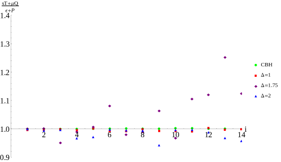
Figure 1: Verifying Euler relation: the horizontal axis is a solution index

Hence, in what follows - we simply determine the energy numerically by using the Euler relation and the conformal equation of state $E=(d-1)PV$ as $\epsilon=\frac{d-1}{d}(Ts-\mu\rho)$.

The action of the bulk theory when evaluated on the solutions is interpreted as a thermodynamic potential of the boundary theory. However one must add counterterms (living entirely on the boundary thereby not affecting the equations of motion) to ensure that the divergences coming from integrating upto $z=0$ cancel. A simple approach is to use a minimal subtraction scheme which ensures cancellation of only the divergent terms. A more sophisticated approach is to use the method of “holographic renormalization” Skenderis .

We find that neither of these approaches is numerically tractable for similar reasons as mentioned in the evaluation of the energy. The integration of the gravity part of the action turns out to be extremely sensitive to the cutoff and ensuring that the numerical values are insensitive to the choice of cutoff proved well-nigh impossible.

However, not all is lost - using the Euler relation above the grand potential is simply the negative of the pressure which can be determined directly from the energy by using the equation of state relating the pressure to the energy density.

Since the particle number is computed by using Gauss’ law, we can calculate the number of particles carried by the black hole alone by evaluating the electric flux at the horizon. In the dual theory, this maybe interpreted as the number of particles occupying the excited states of the single particle spectrum (although this may not be sensible when the particles are strongly interacting). From the field theory point of view, the interpretation of the condensate as the occupancy of the ground state of the single particle spectrum has been a source of some tension because of thermal fluctuations (and especially interaction effects). This ambiguity in the separation of the total particle number is also visible in the holographic dual. Assuming the field theory dual to live at the boundary, it is unclear if the electric field at the horizon (located in the interior of the asymptotic spacetime) is an independent observable of the boundary theory. Due to quantum effects, particles will be exchanged between the scalar field and the black hole through “Hawking radiation” and infall similar to what happens in the two-component model of a superfluid. The electric flux at the boundary of AdS however suffers from no such ambiguities and is directly interpretable as the total number of particles.

4 Entropy and the microcanonical ensemble

We start by discussing the behaviour of the entropy of the system as a function of the extensive variables: the total energy $E$ and the total number of particles $N$ - namely, the fundamental thermodynamic relation. The energy and the number of particles are the natural variables characterizing the system in the microcanonical ensemble. Note that the field theory coordinates $x,y$ span an infinite volume in units of the radius $L$ of AdS (which has been set to unity). Hence, the appropriate variables are the energy density $\epsilon=E/V$ and the number density $\rho=N/V$.

Firstly, we shall identify the space of solutions of gravity system corresponding to various thermal states of the dual field theory. In the absence of the condensate, we have a thermal gas of particles in the field theory which is described by a charged AdS black hole Chamblin , with the energy density $\epsilon$

$$\epsilon=\frac{(d-1)}{4\pi}(4G_{N}s^{d})^{\frac{1}{d-1}}(1+\frac{(d-2)}{32q^{2}(d-1)G_{N}^{2}}\frac{\rho^{2}}{s^{2}})$$ (6)

exhibiting two different power laws at either extremes, depending on the ratio dimensionless $\frac{\rho}{s}$. What is not obvious from this expression is that the density is bounded $0<\rho<\rho_{M}$. From the gravitational point of view, this is due to the extremality limit - it is not possible to ’overcharge’ ($M_{bh}<Q_{bh}$ in appropriate units) a black hole.

These solutions fill out the region in white in Fig: 2 where the dot-dashed line in black shows a family of charged black hole (CBH) solutions of varying energy at fixed density. In the figure, the upper boundary of the white region corresponds to $\rho=0$, corresponding to neutral black holes. The lower boundary of the white region corresponds to extremal black holes $\rho=\rho_{M}$ without a condensate, that is to say charged black holes with $T=0$. Below this region, there are no black hole solutions without a scalar field component. From the point of view of the dual system, the extremal black holes are a bit of a puzzle since they have nonzero entropy at zero temperature. This violation of Nernst’ law implies that these black holes cannot be the correct description of the phase of this system at low entropies.

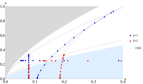
Figure 2: Entropy density vs Energy density

On the other hand, for sufficiently large density (or chemical potential), we have solutions with a condensate - represented on the gravity side by solution with a nonzero profile for the scalar field. These solutions fill out the region in blue in the figure. Two such families of solutions are shown as a pair of solid curves in red and blue at the same total number density as the black dot-dashed curve. The line in blue represent solutions with a $\Delta=1$ condensate and a black hole while the line in red involves the $\Delta=2$ condensate (all for the same total particle density). It is seen that the condensate solutions ”continue” the black hole curve upto $s=0$. It is evident that the onset of condensation occurs much earlier in energy for $\Delta=1$ than for $\Delta=2$. The figure, Fig: 2 suggests that entropy and the slope (i.e., temperature) are both continuous, which would imply that the condensation transition is continuous.

In the figure the row and column of (blue and red) dots, represent points with the same value of $\rho$ but varying condensate value. The blue and red dots represent condensation of operators of scaling dimension $\Delta=1$ and $\Delta=2$ respectively. The uppermost (and leftmost) points correspond to the onset of condensation. Note that the onset of condensation does not extend into the upper grey region of neutral black holes as expected. For the charge cloud to be stable and located away from the black hole, the gravitational attraction of the black hole needs to be cancelled by a repulsive force. If the black holes are neutral, this is not possible, and the cloud will fall in (thus, one can have different kinds of repulsive forces such as dilaton charges leading to other interpretations on the boundary).

Starting from any one of these solutions, we may use the scaling property 3 to obtain new solutions. These scaled solutions fall on the dashed curves in red and blue in the figure (these were obtained by scaling the leftmost red and blue point with $s=1/4$). It maybe noted that the curves do not cut across regions of different color.

The following conclusions may then be drawn from a study of the space of solutions in the $s-E$ plane (the points listed below apply to the situation where the scaling dimension of the operator undergoing condensation is fixed ):

• For every point in the blue region, there is a black hole condensate solution without a node in the scalar field profile.

• For every point in the white region, there is either a unique charged black hole solution with no condensate, or

  There are two solutions with black holes, one of them with a condensate.

• For any $q$ and $\Delta$, and for constant particle number $\rho$, at high entropy we have only charged black hole solutions without any condensate. At low enough entropy, solutions with condensates start to appear. There is a small window of entropy and energy where both solutions co-exist after which the charged black hole curve terminates at an extremal charged black hole. However, solutions with a condensate continue further upto $s=0$ (see the solid curves in Fig: 2).

• It is also seen that for a fixed entropy, $s=1$ say, the solutions with a condensate exist beyond a critical value of energy $\epsilon_{c}$. These solutions are represented by horizontal sequence of blue and red dots in figure Fig: 2. It maybe noted that the $\Delta=1$ dots (in blue) start closer to the neutral black hole boundary (grey region) compared to the $\Delta=2$ dots (in red) that start closer to the extremal black hole i.e., critical value $\epsilon_{c}$ at which condensation starts increases with $\Delta$.

• Conversely, for a given value of $E$, there exist condensate solutions below a critical value $s_{c}$ of entropy. The critical value decreases with the scaling dimension and the temperature is correspondingly lowered. These are demonstrated by the vertical sequence of points marked in blue and red in the Fig: 2.

• Since the curves “end vertically” the slope $\frac{\partial s}{\partial\epsilon}=\infty=\frac{1}{T}$ verifying Nernst’ law. For a given value of the number of particles $\rho$, the larger values of $\Delta$ have larger energies at $T=0$ which is the intersection point of the constant $\rho$ curves with the E-axis.

• A plot of the entropy vs temperature at constant particle number is shown in Fig: LABEL:sTQ where the green curve represents the charged black hole solutions. The solutions with a condensate branch off at different values of $T_{c}$ for the different scaling dimensions - the lower values condensing earlier.

  This figure shows that upon the inclusion of the condensate solutions, the entropy of the system smoothly goes to zero at absolute zero temperature satisfying the Third law of Thermodynamics (which the charged black holes by themselves fail to obey). The location of the horizon of the black hole moves deeper into the bulk of AdS at lower temperatures thereby decreasing the entropy, while the $T=0$ system has no black hole.

• Since entropy and temperature are continuous at the onset of condensation - this transition is smooth without any latent heat. However, the derivative of the entropy jumps at condensation - implying a discontinuity in the specific heat.

  Because of the underlying conformal symmetry, we have an equation of state $p=\epsilon/2$ ($d=3$) which implies that $\epsilon_{0}$ is also the degeneracy pressure (i.e., pressure at zero temperature).

• Plotting the entropy (Fig: LABEL:sQe) as function of the density holding the energy fixed again shows that the entropy goes to zero smoothly as $T$ goes to zero (the graphs “end vertically” on the x-axis).

• At a given energy (for the same number density), once condensation occurs - the solution with the condensate always has higher entropy numerically and is thus the preferred phase (for all values of $q$ and $\Delta$). This is seen by comparing the dot-dashed curve with the red (or blue) solid curves in Fig: 2 (the latter correspond to condensates with $\Delta=2,1$ respectively)- for any given energy, the solid curves are always above the dot-dashed curve.

  In gravitational terms, this statement translates into saying that the area of the (charged) black hole increases once the cloud of charge represented by the scalar field appears (at fixed number density for low enough energy or for high enough density at fixed energy). Lowering the total energy of the system is achieved by moving charge out of the black hole into the scalar cloud surrounding it - assuming that the cloud models ground state occupancy in the usual picture of Bose condensation. This process seems to have a smaller electrical effect than gravitational (then, the horizon moves closer to the boundary, decreasing $z_{H}$ thereby increasing the entropy). This conclusion is not obvious since one could have expected that the small charge on the cloud can only repel the black hole pushing the horizon further into the bulk.

• The power-law behaviour of energy as a function of temperature is shown in Fig: 5 - the lower curves represent the specific heat (scaled by a factor of ten) which is the derivative of the energy.

  

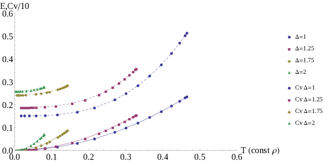
  Figure 5: $\epsilon,\frac{C_{V}}{10}$ vs T for constant $\rho$

  The discontinuity in the specific heat maybe seen in the graph of the energy density (at constant number density) Fig: 5 - the finite discontinuity in the specific heat is markedly different from the lambda transition of superfluid liquid helium.

• As shown in Fig: LABEL:muqe, the chemical potential turns out to be linear function of the charge density. In the absence of the condensate, i.e., for the charged black hole alone, the bulk gauge field is a linear function of the holographic direction $z$, and imposing the boundary condition that $A_{0}(z_{H})=0$ gives a linear relation between $\mu$ and $\rho$ (see Appendix). Once the scalar field is present, the gauge-field profile in the z-direction is no longer linear. The nearly linear behaviour of the chemical potential is surprising because in the bulk language this means that the scalar cloud hardly affects the bulk gauge field profile. Of course, the equivalent statement in the usual understanding of condensation is that the chemical potential contribution of the condensate is zero.

  Considering the range that the data cover in Fig: LABEL:muqe from the onset of condensation at $\rho=\rho_{c}$ to $T=0$, the density varies by a factor of two for small $\Delta$, whereas for the larger $\Delta$, the density hardly changes.

  A similar statement obtains for the energy variation suggesting that for larger scaling dimensions, most of the states undergoing condensation at finite temperature are from occupied states near the ground state.

• To conclude, we show the behaviour of the condensate (order parameter VEV) in Fig: LABEL:oqe; the numerical data can be fit by a functional form $\mathcal{O}=\mathcal{O}_{0}\sqrt{\frac{\rho}{\rho_{c}}-1}$. We shall return to this in section 6. However, the large difference as we vary the scaling dimension is noteworthy.

4.1 Entropy and condensation

Once we know that condensation occurs, we can plot the entropy of the system as a function of the total number density (at fixed temperature). We may expect that, if the system were bosonic, the entropy saturates because the added particles occupy the ground state. This is shown in Fig: LABEL:sqT - where we normalize the entropy by the charge on the black hole $\rho_{T}$. This figure shows that the entropy varies but little - most of increase in the number density is added to the condensate which indeed contributes little to the entropy.

The charge in the scalar cloud resides close to the horizon for larger scaling dimension system- whereas for the smaller, the charge is more distributed (see section 6.4). This is easily understood from a Frobenius analysis of the bulk equations. In the holographic dictionary, the radial direction corresponds to energy scales of the dual system. This means that the particles in the condensate are, on the average, more dispersed in energy for smaller scaling dimension as might be expected.

In the usual AdS holographic dictionary, the entropy of the boundary theory is mapped to the area of the horizon of a black hole that is present far in the interior of AdS space. However, this horizon area when “pulled back” onto the boundary (so that it is a boundary observable) could be expected to be “distorted” or lensed by the energy density present in the scalar field profile in the intervening region. If this happens, this is the gravitational interpretation of entropy production/reduction. Thus, it is interesting to ask whether the entropy is affected by the presence of the condensate. The field theory interpretation would suggest that the entropy remains nearly constant (the interaction (thermal loops) between the condensate and the thermal cloud could alter this expectation). In the AdS side, we therefore vary the total electric charge while keeping the charge on the black hole fixed (thus only the number density in the condensate changes).

In Fig: LABEL:sbyrho, we see that the entropy density remains nearly constant over a large range of total charge (for fixed charge on the black hole which we take to represent the thermally excited population $\rho_{T}$).

The minima in this fixed temperature graph shows that for low electric charge in the condensate cloud, the Coulomb repulsion leads to decrease in horizon area (the horizon is ’repelled’ from the boundary), (Fig: LABEL:sbyrho) - but clearly gravitational attraction dominates at large condensate density since the entropy eventually increases. Note that, for larger values of the scaling dimension, the minima seems to be disappear.

It will be interesting to understand the minima entirely from the dual field theory perspective. Gravitational attraction and Coulomb repulsion in terms of field theory?

This has the interpretation of a thermodynamic process which changes the number of particles in the condensate while keeping the number of particles in the thermal cloud fixed. This process deserves to be studied better perhaps along the lines of Sonner:2014tca since it seems like one is probing the change in a quantum state (the condensate) which is interacting with a thermal bath. The entropy changes observed must be because the energy (temperature) stored in the cloud undergoes a change due to addition of particles in the condensate.

At a given energy where black hole solutions coexist with solutions with condensates, the solutions with a condensate have higher entropy (see Fig: 2). The process of condensation involves moving charge from the black hole into the scalar cloud surrounding it. This leads to an increase in entropy because the entropy of the black holes increase as the density decreases at fixed energy.

In this process, since $\delta E=0$,

$$0=\delta E\geq\delta\rho_{cond}E_{0}+\delta\rho_{T}E_{1}=\delta\rho_{tot}E_{0}+\delta\rho_{T}(E_{1}-E_{0})$$

with $E_{1}>E_{0}$. Here $E_{1}$ is the energy of the first excited state (in the single particle language) from which particles are removed (which is likely the highest occupied state). From this we get, $|\frac{\delta\rho_{cond}}{\delta\rho_{T}}|\geq\frac{E_{1}}{E_{0}}$   ($\delta\rho_{T}<0$) which implies that if the (absolute value) of the slope of the graph of $\rho_{cond}\,{\rm vs.}\,\rho_{T}$ is greater than unity (at $T=0$), this indicates a gapped system.

These graphs for various scaling dimensions are shown in Fig: 10 along with a dashed (red) line line of unit slope. We immediately observe that the near zero temperature values of $\rho_{cond}$ (y-intercepts) are greater than the corresponding x-intercepts which represent the initial population in the thermally excited states. From a visual comparison, it is seen that the slope of all curves is greater than unity (in the lower part of the curve near $T_{c}$). However, we note that near the y-axis, the slope is nearly unity at $T=0$ indicating the absence of an energy gap.

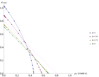
Figure 10: Occupancies of the condensate vs. excited states at fixed energy E

Note that at zero temperature, all the electric charge resides on the condensate (and there is no black hole in the bulk). Gubser:2008pf -Horowitz:2009ij . Thus, all the graphs intersect the y-axis at nonzero values of $\rho_{cond}$. For a given energy, the amount of $\rho_{cond}$ decreases with the scaling dimension. This is as expected since the higher scaling dimension operators create states of higher energy in the field theory. On the other hand, the onset of condensation is represented by the x-intercept which shows a systematic increase with the scaling dimension of the operator that undergoes condensation also as expected. Fixing the total energy, we can note that for smaller $\Delta$, the number of particles occupying the condensate at $T=0$, is nearly double that in the thermal gas at $T=T_{c}$ in contrast to the larger $\Delta$. This suggests that most of the particles in the larger $\Delta$ systems are near the ground state (so that energy changes only by little when these condense).

5 Grand Canonical Ensemble: Chemical potential and equation of state

In the grand canonical ensemble, thermodynamic states are labeled by the chemical potential and temperature. Therefore, to begin with, we try to understand how the various solutions cover the quadrant $T>0,\mu<0$. In Fig: 11, the radial lines represent families of solutions obtained by the scaling transformation, eqn: 3, starting from any one of the solutions (represented by colored dots) on that ray. We obtain straight lines because both $\mu$ and $T$ having dimensions of energy, transform in the same way under scaling.

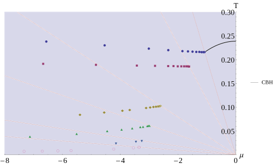
Figure 11: $\mu$ vs T for $s=\frac{1}{4\pi}$

The solid black curve represents charged black holes without a condensate and dots represent solutions with a condensate - all these points have entropy density $s=1$. The various radial rays are critical lines to the right of which there are NO solutions with a condensate of that scaling dimension. For instance, in the region to the right of the right most ray - there are no solutions with condensates for scalar fields with scaling dimensions $\Delta>1$. The blue dots representing the $\Delta=1$ condensates make their first appearance on this ray; In this region, there are only black holes without condensates (for the $\Delta=1$ operator) - there could be operators of lower scaling dimension that could also condense. To the right of the second most ray there are no solutions for scaling dimensions $\Delta>5/4$ etc. As the scaling dimension increases, the condensate solutions appear at larger (negative) values of the chemical potential.

In the same figure, we see that, for fixed $\mu$ and $\Delta$, a condensate solution always appears at low enough temperature (this occurs at the intersection of the constant $\mu$ line with the ray corresponding to the particular $\Delta$ chosen). The temperature at which condensate solutions can be found decreases for large scaling dimension, while for small scaling dimension, this critical temperature actually increases. Note that in this figure, entropy is being kept constant.

Thus, we see that for most of the quadrant the CBH solutions co-exist with the condensate solutions. In this region, the question of which phase dominates is then decided by the system having larger pressure (lower grand potential). This is quite different from the micro-canonical ensemble where the coexistence region is very small.

From the perspective of the microcanonical partition function

$$\frac{\mu}{T}=-\log\frac{\Omega(E,V,N+1)}{\Omega(E,V,N)}$$

Thus, $\mu$ represents the cost of adding a particle to the system while keeping the thermodynamic internal energy $E$ constant. We may interpret the higher energy cost for higher scaling dimension condensates as being due to these being composite operators in terms of single particle states.

At fixed number density after the onset of condensation, in sharp contrast to the bare black hole, it is seen that the chemical potential hardly changes. In any case, at $T=0$, we may expect that the distinction between chemical potential and the ground state energy disappears. This is indeed the case as shown by the graph in Fig: 12 where the ratio of the energy per particle to the chemical potential is plotted as a function of the temperature.

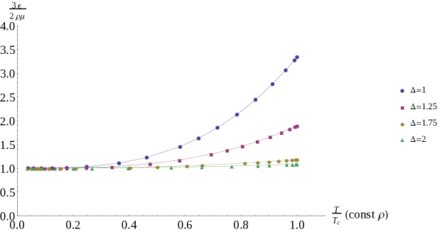
Figure 12: $\frac{3\epsilon}{2\mu\rho}$ vs T at constant $\rho$

Note that at zero temperature, since the entropy goes to zero, because of extensivity and the equation of state, the ratio $\frac{\epsilon}{\rho\mu}\to\frac{d-1}{d}$ - which is an artifact of the conformal symmetry.

5.1 Equation of state

As mentioned earlier, a consequence of conformal invariance is the tracelessness of the stress tensor of the field theory which leads to the equation of state $\epsilon=(d-1)p$. In the grand canonical ensemble, we have another equation of state relating $\mu$ with its thermodynamic conjugate, the number density $\rho$ (for fixed $T$ or $\epsilon$).

Using extensivity, we can see that the equation of state takes the form $\mu^{2}=\rho\,f(\frac{T^{2}}{\rho},\Delta)$ (in $d=3$ again assuming analyticity in $T$). The dependence on temperature however must be determined numerically. Fig: LABEL:qmuT shows that in fact, $\mu^{2}/\rho$ is nearly independent of $\rho$ when there is a condensate (the dashed curves represents the equation of state obtained from a charged black hole) The constant seems to depend mildly on the scaling dimension with larger scaling dimensions having more negative chemical potential values.

The phase diagram of the Einstein-Maxwell system alone was studied a long time ago (for spherical boundary topology) Chamblin where it was observed that the charged black holes do not represent the low temperature phases. The solutions with a condensate fill out the low temperature region as seen in the graph of the grand potential as a function of the temperature (for fixed chemical potential). Similar to the canonical ensemble, the solutions with a condensate represent the stable phase with a lower grand potential compared to the corresponding black hole. As before, the phase transition is continuous.

6 Dependence on the Scaling dimension

In this section, we shall focus on the dependence of various thermodynamic properties on $\Delta_{-}$ defined as the scaling dimension of the operator that undergoes condensation.

6.1 Power laws and Thermostatics

The shape of the entropy curves (Fig: 2, Fig: LABEL:sTQ) suggests power law dependencies on the independent variable. Thus we attempt to fit $s=s_{0}(\epsilon-\epsilon_{0})^{\alpha}$ to our numerics, where the constants $s_{0},\epsilon_{0}$ are functions of both $\Delta$ and $q$ as well as the density $\rho$ (which is being kept constant).

Such a fitting form is also suggested by experiment (for instance, Luo:PRL ) where it is found that the entropy for ${\rm Li}^{6}$ atoms in a trap could be fitted with the formula $s=s_{0}\left(\frac{\epsilon-\epsilon_{0}}{\epsilon_{F}}\right)^{\alpha}$ with an exponent $\alpha=0.6$. Their system thus behaved like a degenerate Fermi gas and $\epsilon_{F}$ was interpreted as the Fermi energy while $\epsilon_{0}$ is the ground state energy per particle.

The comparison with the holographic system must be made with circumspection: the holographic system is both conformal and relativistic - although both these symmetries are broken by the temperature and chemical potential. The dual boundary system lives in 2 noncompact dimensions whereas the above experiment is in a trap in 3D. Nevertheless, the interpretation of $\epsilon_{F}$ is likely to be profitable.

From the expression for entropy, we can obtain the dependence of the energy on temperature by inverting the equation $\frac{1}{T}=\frac{\partial s}{\partial\epsilon}$. Thus, $\epsilon=\epsilon_{0}+(\frac{\epsilon_{F}^{\alpha}}{\alpha s_{0}})^{\frac{1}{\alpha-1}}\,T^{\frac{1}{1-\alpha}}$ and hence the exponent for the specific heat is determined $c_{v}\sim T^{\frac{\alpha}{1-\alpha}}$.

It is noteworthy that we obtain an excellent fit to the numerical data with the above fitting form. The best fit values for the parameters of the fit are shown in Fig: LABEL:seFit and the Table: LABEL:TablesE above. The graph shows that the exponent varies from nearly $\alpha=2/3$ for $\Delta=1$ to $\alpha=1/2$ for large $\Delta$. Note also that the energy per particle increases with the scaling dimension, but seems to be saturating for large $\Delta$.

For the dependence of the entropy on the density (keeping the energy held constant), the expression $s=s_{0}\left(\frac{\rho_{0}-\rho}{\rho_{0}-\rho_{c}}\right)^{\beta}$ fits the data near the onset of condensation $\rho_{c}$ (but deviates somewhat near $T=0$ for the smaller scaling dimensions). In the table LABEL:srtable, we show the best values of $\rho_{0}$ and $\beta$ as well as the values of the critical density $\rho_{c}$ (note that both $\rho_{0,c}$ depend on the constant energy). The accompanying graph shows the ratio of $\frac{\rho_{0}}{\rho_{c}}$ which illustrates the large variation with the scaling dimension.

The exponents in the two tables above agree reasonably well.

We can read off the ground state energy per particle from the y-intercept in the graph Fig: 10, or equivalently from $\epsilon_{0}=\frac{\epsilon}{\rho_{0}}$ where $\epsilon$ is the constant energy at which Table: LABEL:srtable was obtained. This can be compared with the zero temperature value as mentioned in Table: 6.1 (keeping in mind that the different density used for the latter table). These different evaluations agree to numerical accuracy (as they must).

In the canonical ensemble, we can numerically fit a polynomial to the $\epsilon$ vs $T$ points and from this obtain a graph of the specific heat itself - this was shown in Fig: 5. The specific heat behaves as $C_{v}\sim T^{\sigma}$ as shown in the table below - where one can see that the ground state energy $\epsilon(T=0)$ scales (nearly) linearly with the scaling dimension. These values for the ground state energy and exponents agree with those obtained from the $s$ vs. $\epsilon$ curves (as they must) $\sigma=\frac{\alpha}{1-\alpha}$.

$\Delta$	$\epsilon$	$\tilde{\epsilon}_{0}$	$\epsilon_{F}$	$\frac{\rho_{0}}{\rho_{c}}-1$	$\mathcal{O}_{0}$	$\sigma$
1	$0.15+3.6T^{\sigma+1}$	0.19	0.29	1.265	4.7	2.06
5/4	$0.19+4.8T^{\sigma+1}$	0.22	0.25	0.552	5.6	2.03
7/4	$0.24+14.5T^{\sigma+1}$	0.27	0.143	0.113	21	1.6
2	$0.26+37T^{\sigma+1}$	0.29	0.09	0.049	67	1.3

We also showed the dependence of the order parameter on the density (keeping $\epsilon$ fixed) in Fig: LABEL:oqe. The vev is well fitted by curves of the form $\langle\mathcal{O}\rangle=\mathcal{O}_{0}\sqrt{\frac{\rho}{\rho_{c}}-1}$ where the constant $\mathcal{O}_{0}$ is shown in Table: 6.1. The order of magnitude difference in the prefactor $\mathcal{O}_{0}$ (Table: 6.1) between the lower scaling dimensions and the higher ones is noteworthy - a similar such difference was pointed out as defining either sides of the BEC-BCS crossover in Stringari . Such a large difference was also observed in the earlier work KKY in the condensate fraction in the core of vortices and dark solitons.

6.2 Onset of Condensation

We plot the value of $T_{c}$ at which condensation starts as a function of scaling dimension while keeping the chemical potential fixed. For a given $\Delta$, as $q$ increases the onset of condensation $T_{c}$ also increases for fixed $\mu$. For larger $\Delta$, the the temperature of onset decreases as expected.

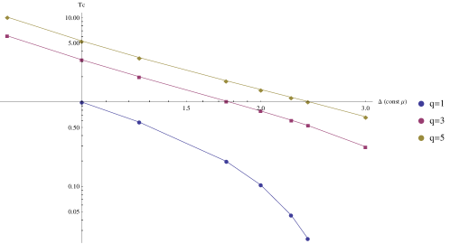
Figure 17: $T_{c}$ vs. $\Delta$ at constant chemical potential

Our proposal is to compare this graph with computations of the variation of the condensation temperature with the interaction strength as in for instance cold atom systems what or neutrons Sunethra . In these systems, the possibility of BEC-BCS crossover leads to the presence of a new energy scale, namely the Fermi energy (apart from the healing length). Such a possibility was already explored earlier in KKY where the core densities of solitons were argued to show signs of a Fermi energy.

On dimensional grounds, the appearance of a new length scale might be expected to alter the functional dependence of $T_{c}$ on $\Delta$. In the graph of $T_{c}$ vs $\Delta$, which is shown on logscale, we can see that for large $q$ where the back-reaction of the scalar cloud is insignificant, the $T_{c}$ is a power of $\Delta$.

But, for $q=1$, where the back-reaction plays a significant role, we might want to see a difference arising for $\Delta>=2$. Such a change in character maybe attributed to a new scale either arising or disappearing - but the graph is not conclusive.

6.3 Joule Thomson Coefficient

From Fig: 11, where one sees two different slopes for the chemical potential graphs, one might be tempted to infer a qualitative difference. This difference is clearly visible in a graph of how the density changes while adiabatically (keeping entropy constant) changing the temperature - i.e., the coefficient of volume expansion. The $\Delta=1,1.25$ curves show a monotonic increase in the density at fixed entropy whereas the $\Delta=2,2.25$ show a decrease. For $\Delta<\frac{d}{2}$ the chemical potential decreases (becomes more negative) as the temperature decreases (with entropy fixed), whereas for $\Delta<\frac{d}{2}$, the chemical potential increases (the solutions for $\Delta=0.75$ are numerically inaccurate). Contrast these with the behaviour of the chemical potential for the charged black holes without any condensate - which is the flat horizontal curve towards the bottom of the graph.

From this one can obtain the Joule Thomson coefficient $\mu_{JT}=\frac{1}{\rho}\frac{d\rho}{dT}|_{s}$. In a graph of the density against temperature at constant entropy, the regions where the slope is negative is the region where cooling occurs upon expansion.

As seen in the graph, for small $q\sim 1$, the large $\Delta$ superfluid undergoes cooling upon expansion. Whereas, for either small $\Delta$ or for large $q$ (and any $\Delta$), expansion is accompanied by temperature increase. The horizontal curve is the expansion coefficient of the black hole. This curve terminates at the rightmost point.

On the other hand, consider the slope $\left(\frac{\partial s}{\partial\epsilon}\right)_{T}=\frac{\left(\frac{\partial s}{\partial\rho}\right)_{T}}{\left(\frac{\partial\epsilon}{\partial\rho}\right)_{T}}$. Since the temperature is fixed, the property that is being varied is the number of particles. From the graph (Fig: LABEL:esT), it is clear that entropy decreases for the $\Delta<\frac{d}{2}$ by adding particles. This is possible only if there was an attraction between the particles - because the decrease in entropy can only mean a decrease in phase space volume which is possible if the particle motions are somehow restricted.

In contrast, the higher scaling dimensions show an initial repulsion which would lead to the added particles occupying a larger phase space volume leading to an increase in entropy. Note that eventually (at large densities) we expect that all additional particles occupy the ground state and so the entropy will end up at some nonzero value due to the constant (nonzero) temperature.

6.4 Solution profiles

The features described above maybe traced back to the properties of the gravitational side of the hologram by considering the bulk equations 2. Asymptotic analysis tells us that $\psi\sim z^{\Delta_{-}}$ 5 near the boundary. Thus, the electric charge density in the scalar field, expressed as $\rho(z)=\frac{\psi^{2}A_{0}h}{gz^{2}q^{2}}$ gets pushed away from the boundary as the scaling dimension increases (Fig: LABEL:charged) because the electric scalar potential in the bulk is essentially linear (and vanishes at the horizon).

The behaviour of the bulk metric on the other hand, carries information about the temperature. In this case, increasing the charge in the scalar field near the horizon will decrease the curvature $g^{\prime}_{00}$ of the metric as we can see from the gravity equations in 2. For small scaling dimensions on the other hand, any extra charge is pushed out close to the boundary as seen in Fig: LABEL:charged - thus having small effect on the metric near the horizon. For larger scaling dimensions, the extra charge localizes near the horizon Fig: LABEL:charged and hence this leads to a much larger decrease in slope leading to very low values for the temperature. Note that this effect of the charge competes with the increase in $g^{\prime}_{00}$ due to the $dz$ term in 2 which is present even for the black hole without any scalar field.

In Fig: LABEL:g00, we see that the metric profile for small scaling dimensions (the curves drawn in blue) is similar to the metric of the charged black hole without a condensate (the outermost blue curve). However, for large scaling dimensions and larger values of the condensate, $g_{00}$ flattens out in the region near the horizon. For each scaling dimension (as indicated in the legend), we have shown a pair of curves - the outer curve having lower value of the condensate. We also see that the even for moderate condensation, the second derivative $g^{\prime\prime}_{00}$ differs in sign for the larger scaling dimensions (turns positive) compared to the smaller ones (remains negative). Presumably, this is the reason behind the differing properties of the large and small scaling dimensions.

This does not explain the subsequent increase in temperature for the smaller scaling dimensions (Fig: LABEL:JT). Also, the temperature increases with $\rho$ for large $q$ independent of the scaling dimensions. Presumably, in this range, the temperature is not affected much by the scalar cloud since the fraction of charge contained in the cloud is small as compared to the black hole charge. Thus, the behaviour is essentially that of the charged black hole.

Further, moving some electric charge from the black hole into the scalar cloud keeping the total charge fixed leads to an initial increase in energy (from the coulomb repulsion). But, eventually the Coulomb repulsion cost attains a maximum since as far as the electric charge is concerned, the scalar cloud and black hole are symmetric. Thus, at fixed entropy, energy of the system decreases when electric charge is transferred from the black hole to the scalar cloud. The amount of decrease in energy is less Fig: 2 for the smaller scaling dimensions since, for these, the electric charge is more delocalized in the bulk (note that in Fig: 2, the total density is being varied).

Above, we attempted to explain the observed features of the system entirely in the language of the bulk gravitational system. We might expect that these “bulk explanations” can be translated entirely into the language of the boundary theory. In this context, one might expect that the interpretation of the radial direction as the (renormalization) scale of the field theory could play a role as well.

6.5 Order parameter

The condensate order parameter - which is the vacuum expectation value of the operator that breaks the $U(1)$ symmetry spontaneously, shows the characteristic behaviour as demonstrated in other works- except that we may notice a systematic increase in the zero temperature value with the scaling dimension. The figure Fig: LABEL:vvevT also includes $\sqrt{1-x^{\nu}}$ best-fit curves with exponents as indicated in the plot legend and the order of magnitude difference between $\Delta>\frac{3}{2}$ and $\Delta<\frac{3}{2}$ maybe noted. Another feature is the trend as $\Delta$ increases. For $\Delta=1,5/4,7/4$ the exponent decreases with increasing $\Delta$ whereas for $\Delta=2,9/4,12/5$ the exponent increases (the data for $\Delta=9/4,12/5$ are close enough to be fit with either exponent, but in any case we recall that $\Delta=9/4$ data is numerically inaccurate).

6.6 Compressibility

Observing that the number density (Fig: 10) or condensate (Fig: LABEL:vevT) at zero temperature is much larger for the smaller scaling dimensions leads us to compare the compressibility of the various cases. The larger occupancy suggests that the compressibility is larger.

We can obtain both isothermal and adiabatic(isentropic) compressibilities defined as

$$\kappa_{T,S}=-\frac{1}{\rho}\frac{d\rho}{dP}$$

from the numerical solution. The isothermal graph of pressure vs. density is shown in Fig: LABEL:comp (note the log-scale) along with best fit curves of the form

$$P=P_{0}\rho^{\frac{3}{2}}$$

.

From these, we may extract the isothermal and adiabatic compressibilities, and obtain the ratio $\frac{\kappa_{T}}{\kappa_{S}}$. This ratio should be greater than unity - in fact, one can define an effective number of degrees of freedom $d_{f}$ by $\frac{\kappa_{T}}{\kappa_{S}}=1+\frac{2}{d_{f}}$. For all values of $\Delta$, our numerical accuracy does not distinguish $\kappa_{s}$ and $\kappa_{T}$ and so the number of degrees of freedom is essentially infinity. For this to be deemed sensible, we should be able see that $d_{f}$ tracks finite N corrections as befits a holographic interpretation (perhaps, this be done for charged black holes alone) .

A second feature that is noteworthy is the behaviour near the bottom end of the graph (at low densities) which is near $T_{c}$. The compressibilities are clearly becoming larger (pressure is becoming constant) - perhaps it might be worth exploring if the compressibility actually diverges.

7 Dependence on q

In this section, we shall study how the above features vary as we vary the parameter $q=\frac{e\lambda}{\sqrt{G_{N}}}$. Since $G_{N}\sim 1/N^{2}$, varying $q$ is interpreted as varying $N$ which is related to number of colors in the gauge theory. The gauge coupling $\lambda$ could be interpreted in a variety of ways as discussed in the introduction. We can also view $q$ as standing proxy for $e$ which characterizes the strength of the interaction between particles in the condensate and the thermal bath. Of course, we may simply take the bulk gravitational point of view in which case $q$ stands in for $G_{N}$.

Each thermodynamic aspect discussed in the previous sections has a corresponding tale to tell as we vary $q$. We shall present only those where the variation with $q$ is either significant or interesting. Since $q$ appears as an overall factor multiplying the matter part of the action, we may expect that thermodynamic quantities involving only the scalar field and Maxwell field will not be significantly affected by variation in $q$. Therefore, we focus on thermodynamic properties involving the metric and a matter field such as entropy vs. number density etc. At large $q$, the matter fields do not affect the gravitational fields - in practice, we see that even for $q\sim 5$, the metric profile is hardly changed by the condensation of the scalar field at moderate values of the density and away from $T=0$.

In each case, we consider the boundary terms at $z=0$ under an arbitrary variation of the bulk fields. If we identify the boundary chemical potential as $\mu=A_{0}(z=0)$, then the number density picks up the $q-$factors $\rho=\frac{1}{q^{2}}A_{0}$ (via the functional derivative $\frac{\delta\log Z}{\delta\mu}=\rho$). We may also identify $\mu=\frac{1}{q}A_{0}(z=0)$ whence $\rho=\frac{1}{q}A_{0}$. In the first case, $A_{0}$ maybe interpreted as the dual of a quark current, since $\rho$ is proportional to $N^{2}$, while in the second case, $A_{0}$ is more like “baryon” current. Similarly, the number $e$ controls the interpretation of the condensate - whether “pairs” ($e=2$) or “single” ($e=1$) particles make up the condensate.

The parameter $\lambda$ has the interpretation of the interaction strength between the particles (after all, it is the YM coupling constant in the bulk). In the superfluid literature, this interaction strength between the particles is tunable (usually with the aid of the Feshbach resonance) and is captured by the scattering length $a$. Unfortunately, all these cases are covered by the same equations of motion - because the parameters appear only in the combination $q$ and clearly modifications of the bulk action are needed to see “subleading” effects.

We begin with the order parameter by keeping the operator undergoing condensation (i.e., $\Delta$) fixed and varying the coupling constant $q$.

The accompanying graph clearly shows the difference in the two families of condensates, there being an order of magnitude difference between $\Delta=1$ and $\Delta=2$ (as observed earlier in KKY ). We have also overlaid best-fit curves $\langle{\mathcal{O}}_{0}\rangle\sqrt{1-x^{\nu}}$.

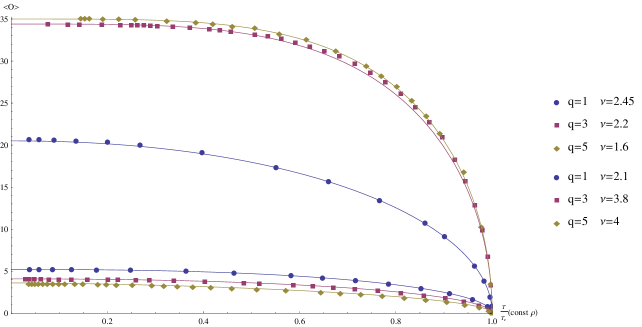
Figure 26: $\frac{<{\mathcal{O}}>}{{\mathcal{O}_{0}}}$ vs $\frac{T}{T_{c}}$ at constant density $\rho$

The larger values of $q$ are closer to the probe limit when the scalar field backreaction can be safely ignored. The probe limit is however attained differently for $\Delta>\frac{3}{2}$ compared to $\Delta<\frac{3}{2}$ (this difference in the behaviour as a function of $q$ was already noted by HHH2 ). Both the exponent and the amount of condensation $\mathcal{O}_{0}$ decrease with $q$ for $\Delta<\frac{d}{2}$ but increase for larger $\Delta$.

Putting together the story for various other values of $\Delta$, we get the following Table: 7 where the trend in both the exponent and the magnitude of the VEV are clearly seen as a function of $q$.

$\Delta\downarrow\,q\rightarrow$	1	3	5	1	3	5
1	2.45	2.2	1.6	5.2	4.08	3.6
$\frac{5}{4}$	2.6	2.8	2.3	4.42	3.67	3.27
$\frac{7}{4}$	2.3	3.7	3.5	8.9	10.5	10
2	2.1	3.8	4	20.5	34.4	35

The first part of the table show the behaviour of the exponent while the second part shows the behaviour of the zero temperature value $\mathcal{O}_{0}$ in $\langle\mathcal{O}\rangle=\mathcal{O}_{0}\sqrt{1-\left(\frac{T}{T_{c}}\right)^{\nu}}$. For any q, it is noteworthy that $\mathcal{O}_{0}$ for $\Delta=2$ is an order of magnitude larger than that for $\Delta=1$.

The energy density continues to behave as $T^{3}$ (at fixed $\rho$) for all values of $q$ except that for larger values of $\Delta$, the energy density goes to nearly zero at $T\to 0$. Correspondingly, the exponents in the entropy vs. density graph (at constant energy) all remain the same at $5/8$ for all $q$ and all $\Delta$.

The entropy density which was a power law of temperature (near $T=T_{c}$) continues to be a power law. However, for larger values of $q$ - the exponents which varied significantly for $q=1$ (see Table: 6.1) become nearly identical at $\alpha=2.25$ (is this the exponent for the black hole?). Of course in the probe limit, the condensation process does not affect the black hole and hence the specific heat becomes continuous as well.

In the case of the entropy as a function of the density (at fixed temperature or thermal density) - we have seen that the entropy decreases initially for the smaller $\Delta$ (Fig: LABEL:sqT). For larger values of $q\geq 2$, the minima disappears, and all curves maybe simply described as a simple power law $s\sim\rho^{\frac{3}{4}}$ (for all $\Delta$).

8 Free energy and Entropy

All along, we have identified the entropy of the dual system with the area of the horizon of the black hole $s=\frac{1}{4\pi z_{H}^{2}}$ . On the other hand, the entropy of the dual system may also be evaluated by considering the Grand Potential $\Omega$ and taking its derivative with respect to $T$–$s=(\frac{\partial\Omega}{\partial T})_{\mu}$ . It will be interesting to ask if these two values agree. In the holographic language, taking derivatives of the grand potential requires us to compare two classical solutions which is similar to considering a (quasi-static) thermodynamic process. Put this way, it is quite non-obvious that these two evaluations will give us the same result, especially because of the presence of the condensate.

To check this, we first use an interpolation function to fit the values $\Omega(T)$ for fixed chemical potential. The numerical derivative $s=(-\frac{\partial\Omega}{\partial T})_{\mu}$ is plotted as a solid curve in the figure 27 against the entropy data obtained from individual solutions as $s=\frac{1}{4\pi z_{H}^{2}}$ shown as dots- showing excellent agreement.

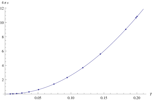
Figure 27: $4\pi s$ vs. T at constant $\mu$ for $q=1,\Delta=1$

Another such thermodynamic relation is $\frac{\partial(\beta\Omega)}{\partial\beta}=U=T_{00}$ - which we show in figure 28. In this graph, we show the energy data points obtained from using the FG-expansion $\epsilon=-\frac{d}{4\pi G_{N}}\frac{2}{3}g^{(d)}_{00}$ (blue dots) as described earlier - along with the energy values determined by using the Euler relation (magenta colored dots). These are shown against the curve obtained by using an interpolating function and differentiating.

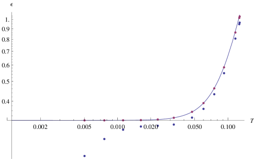
Figure 28: $e$ vs. T at constant $\mu$ for $q=1,\Delta=1$

These equalities are expected if we identify $\log Z=-\beta\Omega$ with the grand partition function. Many other such thermodynamic consistency conditions and relations have been studied/used in works on holographic fluid dynamics and also on holographic sum rules. For the charged black hole alone - these relations can be verified analytically as detailed in the appendix.

9 Discussion

In this paper - we have assembled together a fairly comprehensive treatment of the thermostatic properties of a particular family of holographic superfluid systems. We have shown that upon inclusion of the condensate solutions, a complete phase diagram can be obtained. Here, we focused on the phenomenological differences that occur due to varying scaling dimensions. We have presented a careful exploration of thermodynamic consistency of the holographic recipe - by showing that familiar thermodynamic relations are indeed obeyed by these holographic systems.

A utility of the holographic description is that some of the features of the field theory thermodynamics maybe understood as a competition between gravitational attraction and electric repulsion between the black hole and the charge cloud of the scalar field. Another approach via the Raychaudhuri equations Tian on the gravitational side could lead to further insights on the behaviour of the field theory system - especially from the viewpoint of the quantum to thermal transition that happens when the condensate occupancy is varied keeping the total number of particles fixed. This line of exploration will be able to shed some further light on the condensation of neutral scalars as well.

The dependence of various thermostatic quantities compare favorably with those obtained from experimental systems probing the physics of gases of cold atoms. These comparisons must be approached with caution - since there is scant motivation. However, the holographic graphs do seem to capture interaction effects going well beyond perturbation theory and even mean field theory. Thus, a careful and more comprehensive comparison in four boundary dimensions, this time including transport properties and relaxation time scales might be an exciting place to confront holography with experiments.

In fact, our study has already suggested that isentropic processes maybe able to better capture the effect of the interactions and highlight qualitative differences as we vary the interaction strength. We have also shown that the critical exponent of the order parameter depends on the bulk gauge charge apart from the nature of the order parameter (quantified by the scaling dimension). This latter feature is relevant for further exploration along the lines of holographic QCD equations of state since the gauge field in the bulk gets reinterpreted as giving rise to a flavor symmetry in the boundary. We have also pointed out that for the purpose of phenomenology of these systems, additional (bulk) interactions that break the degeneracy among the parameters $\lambda,e,G_{N}$ will be required. The manner in which $q$ appears in the thermodynamic quantities in the main text suggest specific additional bulk couplings which might be expected to play a significant role (in fact, one should re-examine the literature surveyed in the introduction in this light since significant work has already been done along these directions). We hope to explore a few of these questions in the near future.

10 Charged black hole

In this section, we summarize the thermodynamics of charged black holes in $AdS_{d+1}$ space.

$$\Psi(z)=0\hskip 28.45274pt\chi(z)=4\log z$$ (7)

$$\phi(z)=\mu+Qz^{d-2}$$ (8)

$$g(z)=z^{2}+\frac{(d-2)Q^{2}z^{2d}}{2q^{2}(d-1)}-cz^{2+d}$$ (9)

The parameters $q,Q$ and $c$ determine the temperature of the AdS-Schwarzschild black hole. For positive $c$, is this solution unstable in the usual thermodynamic sense. Note that $c$ also has the interpretation of energy in the dual theory while the condition that the scalar potential vanish at the horizon determines the chemical potential to be $\mu=-\frac{Qz_{0}^{d-2}}{q}$ where $Q$ is related to the number density $\rho$ as $\rho=\frac{(d-2)Qz_{H}^{d-3}}{16\pi qG_{N}z_{H}^{d-1}}$

By rescaling $r=\lambda z$ and defining $\alpha=\frac{(d-2)Q^{2}}{2q^{2}(d-1)}$,

$$g=\lambda^{2}r^{2}(1-c\lambda^{d}(r^{d}-\frac{\alpha\lambda^{d-2}}{c}r^{2d-2}))$$

If we choose $\frac{\alpha\lambda^{d-2}}{c}=1$, this fixes $\lambda$ and the function can be rewritten as

$$g=r^{2}c\lambda^{d+2}(\beta-r^{d}+r^{2d-2})$$

with $\beta=\frac{1}{c\lambda^{d}}$ and hence the root $r_{0}(\beta)$ is a function of the combination $\beta$ alone. The temperature is determined from the conical singularity argument to be

$$T(c,\frac{Q}{q})=\frac{g^{\prime}[r_{0}]\exp[-\frac{\chi}{2}]}{4\pi}=\frac{c\lambda^{d-1}}{4\pi r_{0}}(2\beta-(d+2)r_{0}^{d}+2dr_{0}^{2d-2}))$$ (10)

From the expression for the location of the horizon, we can see that there is a condition $0<\beta<\frac{27}{256}(d=3)$ which in turn means that there is an upper bound on $Q$ given $c,q$. That is to say, for a given energy $c$, the charge density that the condensate free “black hole” can sustain has a limit. This statement can also be translated into the canonical ensemble and maybe said to be the dual of the statement that there is a maximum number density that can be supported by the excited states of a bosonic system at finite temperature (or energy). Increasing the density further could lead to BEC - thus finite occupancy of the ground state. In the AdS side, this means that we have a charged scalar field with a nonvanishing profile.

From the analytic solution, we may extract the following boundary data.

$$\epsilon=\frac{(d-1)}{16\pi G_{N}z_{H}^{d}}(1+\alpha z_{H}^{2d-2})\quad P=\frac{\epsilon}{d-1}\quad\rho=\frac{1}{16\pi G_{N}}\frac{(d-2)Q}{q}$$ (11)

$$s=\frac{1}{4G_{N}z_{H}^{d-1}}\quad T=\frac{1}{4\pi z_{H}}(d-(d-2)\alpha z_{H}^{2d-2})\quad\mu=-\frac{Q}{qz_{H}^{d-2}}$$ (12)

From this data, we can see that the Euler relation $\frac{\mu\rho+Ts}{\epsilon+P}=1$ is trivially satisfied.

References

- (1) S. S. Gubser, Phys. Rev. D 78, 065034 (2008) [arXiv:0801.2977 ].
- (2) S. A. Hartnoll, C. P. Herzog and G. T. Horowitz, Phys. Rev. Lett. 101, 031601 (2008) [arXiv:0803.3295 ].
- (3) S. A. Hartnoll, C. P. Herzog and G. T. Horowitz, JHEP 0812, 015 (2008) [arXiv:0810.1563 ].
- (4) S. A. Hartnoll, Class. Quant. Grav. 26, 224002 (2009) [arXiv:0903.3246 ].
- (5) J. McGreevy, Adv. High Energy Phys. 2010, 723105 (2010) [arXiv:0909.0518 ].
- (6) S. A. Hartnoll, arXiv:1106.4324 .
- (7) S. Sachdev, Ann. Rev. Condensed Matter Phys. 3, 9 (2012) [arXiv:1108.1197 [cond-mat.str-el]].
- (8) A. Adams, L. D. Carr, T. Sch fer, P. Steinberg and J. E. Thomas, New J. Phys. 14, 115009 (2012) [arXiv:1205.5180 ].
- (9) D. Musso, PoS Modave 2013, 004 (2013) [arXiv:1401.1504 ].
- (10) R. G. Cai, L. Li, L. F. Li and R. Q. Yang, Sci. China Phys. Mech. Astron. 58, no. 6, 060401 (2015) [arXiv:1502.00437 ].
- (11) J. McGreevy, arXiv:1606.08953 .
- (12) Stefano Giorgini, Lev P. Pitaevskii, Sandro Stringari, Rev. Mod. Phys. 80, 1215 [arXiv:0706.3360]
- (13) S. Ramanan and M. Urban, Phys. Rev. C 88, no. 5, 054315 (2013) [arXiv:1308.0939 [nucl-th]].
- (14) M. Antezza, F. Dalfovo, L. P. Pitaevskii, S. Stringari Phys. Rev. A 76, 043610 (2007) [arXiv:0706.0601].
- (15) Luo, L.; Clancy, B.; Joseph, J.; Kinast, J.; Thomas, J. E. Physical Review Letters, vol. 98, Issue 8, id. 080402 [arXiv:cond-mat/0611566]
- (16) S. de Haro, S. N. Solodukhin and K. Skenderis, Commun. Math. Phys. 217 (2001) 595 [hep-th/0002230]
- (17) A. Chamblin, R. Emparan, C. V. Johnson and R. C. Myers, Phys. Rev. D 60, 104026 (1999) [hep-th/9904197].
- (18) M. Kruczenski, D. Mateos, R. C. Myers and D. J. Winters, JHEP 0307, 049 (2003) [hep-th/0304032].
- (19) I. R. Klebanov and E. Witten, Nucl. Phys. B 556, 89 (1999) [hep-th/9905104].
- (20) G. T. Horowitz and M. M. Roberts, Phys. Rev. D 78, 126008 (2008) [arXiv:0810.1077 ].
- (21) S. S. Gubser and A. Nellore, JHEP 0904, 008 (2009) [arXiv:0810.4554 ].
- (22) S. S. Gubser and A. Nellore, Phys. Rev. D 80, 105007 (2009) [arXiv:0908.1972 ].
- (23) G. T. Horowitz and M. M. Roberts, JHEP 0911, 015 (2009) [arXiv:0908.3677 ].
- (24) Y. Kim, Y. Ko and S. J. Sin, Phys. Rev. D 80, 126017 (2009) [arXiv:0904.4567 ].
- (25) O. C. Umeh, JHEP 0908, 062 (2009) [arXiv:0907.3136 ].
- (26) S. Franco, A. M. Garcia-Garcia and D. Rodriguez-Gomez, Phys. Rev. D 81, 041901 (2010) [arXiv:0911.1354 ].
- (27) V. Keranen, E. Keski-Vakkuri, S. Nowling and K. P. Yogendran, Phys. Rev. D 81, 126011 (2010) [arXiv:0911.1866 ].
- (28) V. Keranen, E. Keski-Vakkuri, S. Nowling and K. P. Yogendran, Phys. Rev. D 81, 126012 (2010) [arXiv:0912.4280 ].
- (29) F. Aprile and J. G. Russo, Phys. Rev. D 81, 026009 (2010) [arXiv:0912.0480 ].
- (30) Q. Pan, B. Wang, E. Papantonopoulos, J. Oliveira and A. B. Pavan, Phys. Rev. D 81, 106007 (2010) [arXiv:0912.2475 ].
- (31) Y. Brihaye and B. Hartmann, Phys. Rev. D 81, 126008 (2010) [arXiv:1003.5130 ].
- (32) Y. Liu and Y. W. Sun, JHEP 1007, 099 (2010) [arXiv:1006.2726 ].
- (33) C. Charmousis, B. Gouteraux, B. S. Kim, E. Kiritsis and R. Meyer, JHEP 1011, 151 (2010) [arXiv:1005.4690 ].
- (34) D. Arean, P. Basu and C. Krishnan, JHEP 1010, 006 (2010) [arXiv:1006.5165 ].
- (35) G. T. Horowitz and B. Way, JHEP 1011, 011 (2010) [arXiv:1007.3714 ].
- (36) V. Keranen, E. Keski-Vakkuri, S. Nowling and K. P. Yogendran, New J. Phys. 13, 065003 (2011) [arXiv:1012.0190 ].
- (37) M. Edalati, R. G. Leigh, K. W. Lo and P. W. Phillips, Phys. Rev. D 83, 046012 (2011) [arXiv:1012.3751 ].
- (38) Q. Pan and B. Wang, arXiv:1101.0222 .
- (39) O. J. C. Dias, P. Figueras, S. Minwalla, P. Mitra, R. Monteiro and J. E. Santos, JHEP 1208, 117 (2012) [arXiv:1112.4447 ].
- (40) Y. Liu, K. Schalm, Y. W. Sun and J. Zaanen, JHEP 1405, 122 (2014) [arXiv:1404.0571 ].
- (41) D. Arean and J. Tarrio, JHEP 1504, 083 (2015) [arXiv:1501.02804 ].
- (42) N. W. M. Plantz, H. T. C. Stoof and S. Vandoren, arXiv:1511.05112 .
- (43) J. W. Chen, S. H. Dai, D. Maity and Y. L. Zhang, Phys. Rev. D 94, no. 8, 086004 (2016) [arXiv:1603.08259 ].
- (44) O. DeWolfe, O. Henriksson and C. Wu, arXiv:1611.07023 .
- (45) A. Karch and B. Robinson, JHEP 1512, 073 (2015) [arXiv:1510.02472 ].
- (46) Lei Yin, Defu Hou, Hai-cang Ren Phys. Rev. D 91, no. 2, 026003 (2015) [arXiv:1311.3847 ].
- (47) J. Sonner and B. Withers, Phys. Rev. D 82, 026001 (2010) [arXiv:1004.2707 ].
- (48) E. Kiritsis and V. Niarchos, JHEP 1208, 164 (2012) [arXiv:1205.6205 ].
- (49) I. Amado, D. Arean, A. Jimenez-Alba, K. Landsteiner, L. Melgar and I. Salazar Landea, JHEP 1402, 063 (2014) [arXiv:1307.8100 ].
- (50) J. Sonner, A. del Campo and W. H. Zurek, Nature Commun. 6, 7406 (2015) [arXiv:1406.2329 ]
- (51) N. Iqbal and H. Liu, Class. Quant. Grav. 29, 194004 (2012) [arXiv:1112.3671 ].
- (52) S. A. Hartnoll and R. Pourhasan, JHEP 1207, 114 (2012) [arXiv:1205.1536 ]
- (53) B. Ahn, S. Hyun, K. K. Kim, S. A. Park and S. H. Yi, Phys. Rev. D 94, no. 2, 024043 (2016) [arXiv:1512.09319 ].
- (54) Y. Tian, X. N. Wu and H. B. Zhang, “Holographic Entropy Production,” JHEP 1410, 170 (2014) [arXiv:1407.8273 ].
- (55) Mark J. H. Ku, Ariel T. Sommer, Lawrence W. Cheuk, Martin W. Zwierlein “Revealing the Superfluid Lambda Transition in the Universal Thermodynamics of a Unitary Fermi Gas,” Science 335, 563-567 (2012) [arXiv:1110.3309]