A mathematical study of CD8⁺ T cell responses calibrated with human data

Abstract

Complete understanding of the mechanisms regulating the proliferation and differentiation that takes place during human immune CD8⁺ T cell responses is still lacking. Human clinical data is usually limited to blood cell counts, yet the initiation of these responses occurs in the draining lymph nodes; antigen-specific effector and memory CD8⁺ T cells generated in the lymph nodes migrate to those tissues where they are required. We use approximate Bayesian computation with deterministic mathematical models of CD8⁺ T cell populations (naive, central memory, effector memory and effector) and yellow fever virus vaccine data to infer the dynamics of these CD8⁺ T cell populations in three spatial compartments: draining lymph nodes, circulation and skin. We have made use of the literature to obtain rates of division and death for human CD8⁺ T cell population subsets and thymic export rates. Under the decreasing potential hypothesis for differentiation during an immune response, we find that, as the number of T cell clonotypes driven to an immune response increases, there is a reduction in the number of divisions required to differentiate from a naive to an effector CD8⁺ T cell, supporting the “division of labour” hypothesis observed in murine studies. We have also considered the reverse differentiation scenario, the increasing potential hypothesis. The decreasing potential model is better supported by the yellow fever virus vaccine data.

1 Introduction

In response to cognate antigen, a single naive T cell is able to produce multiple subsets of memory and effector T cells of different phenotypes and functional properties [1]. Recent studies suggest that, in humans, this differentiation process follows a linear progression characterised by the following transitions: from naive (N) to stem cell memory (SCM), to central memory (CM), to transitional memory (TM), to effector memory (EM), and to (terminal) effector (or EMRA) (E) T cells [2, 3]. Stimulation by cognate antigen seems to drive less-differentiated cells to generate more-differentiated progeny. Yet, the mechanisms that control the proliferation and differentiation steps during an immune response, from the activation of naive T cells to the generation of memory and effector cells, are not clearly understood [4, 5, 6, 7].

In the case of CD8⁺ T cells, a few of these mechanisms have already been identified and have helped decipher some of the rules that govern CD8⁺ T cell differentiation (see Ref. [4]). This study showed that, after antigenic stimulation, naive CD8⁺ T cells become committed to multiple rounds of division, then differentiate into effector and memory cells. That is, once the parental naive CD8⁺ T cell has been activated, a developmental program is triggered, in which daughter cells continue to divide and differentiate without further antigenic stimulation. Thus, the initial antigen encounter initiates an instructive developmental programme that leads to effector and memory CD8⁺ T cell formation and confers protective immunity [4, 5].

Mathematical models, together with experimental and clinical data, have improved our understanding of CD8⁺ T cell responses and the generation of effector and memory cells during infection. For example, Ref. [8] combines mathematical modelling with experimental data from clinical studies of yellow fever virus (YFV) to explore kinetic details of the human immune response to vaccination. Some important results from this study include: i) the estimation of the doubling time of effector CD8⁺ T cells to be around two days, ii) that the peak of the CD8⁺ T cell-mediated immune response depends on the rate of T cell proliferation, and iii) that the observed expansion of the YFV-specific CD8⁺ T cell population was achieved in fewer than nine cell divisions [8]. The authors made use of a simple mathematical model, based on Refs. [9, 10], to describe the fraction of YFV-specific CD8⁺ T cells in the secondary lymphoid organs (SLOs) and circulation (blood). The model includes migration from SLOs to blood and from blood to tissues, as well as proliferation in the SLOs (before the peak of the response) and death both in the SLOs and in blood, only after the peak of the response. They calibrated their mathematical model with the average (among all patients) fraction of specific CD8⁺ T cells from the YFV vaccine data in Ref. [11] (see Figure 3B in Ref. [11]).

In two other examples of combined experimental and modelling studies, the authors have followed the clonal expansion of transgenic OT-1 cells in mice. Their experiments identified a heterogeneous population of CD8⁺ T cells arising from naive cells during bacterial infection, and showed that the clonal expansion and differentiation of individual naive T cells is highly stochastic [12, 13]. These stochastic events, from multiple individual precursors, gave rise to a robust cellular fate. Mathematical modelling and parameter calibration indicated that CD8⁺ T cells follow a linear developmental path, with long-lived slowly-proliferating cells differentiating to short-lived, highly proliferating cells [12]. Finally, Gong et al. have recently developed a hybrid approach, that uses an agent-based model in the lymph nodes (LNs) and an ordinary differential equation (ODE) model in the blood compartment [14]. This multi-compartmental model considers the following events: the interaction of naive T cells with antigen-bearing dendritic cells (DCs), as well as cellular proliferation and differentiation in two spatial locations (LNs and blood) [14]. The model was calibrated with mice lymphocytic choriomeningitis virus (LCMV) infection data and the authors concluded that the cellular heterogeneity observed can be attributed to the number of antigen-bearing DCs that each naive T cell is responding to [14].

A number of questions about the kinetics of CD8⁺ T cell-mediated immune responses remain unanswered. For example, the sequence of differentiation steps during a CD8⁺ T cell response is unknown: is it from naive to effector to memory or from naive to memory to effector? A related second question is more technical. As human clinical data is usually limited to blood cell counts, how feasible is it to develop a mathematical model with spatial compartments, such as the draining lymph nodes, circulation (or blood) and tissues, that can be parameterised with data from only the blood compartment? Finally, flow cytometry and tetramer staining allow us to identify and measure, within the blood compartment, the fraction of antigen-specific CD8⁺ T cells in the total CD8⁺ T cell population. It remains a challenge to develop mathematical models of the kinetics of CD8⁺ T cell-mediated immune responses that include different CD8⁺ populations (naive, central memory, effector memory and effector) in the three previously mentioned spatial compartments, that can be calibrated with human data.

In this paper, we analyse population-average models of CD8⁺ T cell dynamics that include four cellular populations: naive, central memory, effector memory and effector T cells, and three spatial compartments: the draining lymph nodes, circulation and skin. We note that each CD8⁺ T cell subpopulation is defined in terms of its homeostatic ability to proliferate or not, its survival capability, migration pattern, its division rates in the presence of antigen, as well as the number of divisions required to differentiate (see Section 2.1) [15]. Since our mathematical models will be calibrated with the fraction of total specific CD8⁺ T cells from the YFV vaccine data in Ref. [11] (see Figure 3B in Ref. [11]), our definition of naive, central memory, effector memory and effector CD8⁺ T cells is not based on their expression levels of CD45RA and CCR7 as provided by flow cytometry data [16, 17]. In this sense, our definition of naive, central memory, effector memory and effector CD8⁺ T cells is based on cell function instead of phenotype.

In order to decipher the sequence of differentiation events during an immune response, we first consider the decreasing potential (DP) hypothesis for generating CD8⁺ T cell heterogeneity [12], with differentiation events linked to division [18]. We have made use of the literature to obtain rates of division and death for each human CD8⁺ T cell population subset, as well as naive T cell thymic export rates. Approximate Bayesian computation (ABC) has been used together with the mathematical model and YFV vaccine data from Ref. [11] (see Figure 3B in Ref. [11]) to obtain posterior distributions of the subset of parameters related to the immune response, such as the number of divisions in the differentiation programme, the time to first division, the time to subsequent divisions, the number of specific clonotypes involved in the response, the duration of the immune response, and migration rates. We find that as the number of clonotypes driven to an immune response increases, there is a reduction in the number of divisions required to differentiate from a naive to an effector CD8⁺ T cell, thus supporting the “division of labour” already observed in murine studies [13, 19]. We then consider the increasing potential (IP) hypothesis for generating CD8⁺ T cell heterogeneity [20], and compare it with the decreasing potential model. Mathematical modelling, Bayesian computation and the YFV data provide marginally stronger support for the DP than the IP hypothesis. We have also performed a sensitivity analysis of both models to determine the extent to which the parameters influence the population dynamics and circulatory kinetics of CD8⁺ T cells through the draining LNs, circulation and skin.

The structure of the paper is as follows: Section 2 provides a brief description of the mathematical models used to describe CD8⁺ T cell dynamics (homeostasis, decreasing potential and increasing potential hypotheses), the choice of model parameters and the computational algorithm. We also describe the sensitivity analysis carried out, as well as the YFV vaccination data used to calibrate the models. The results of our study are presented in Section 3, namely model calibration for both DPM and IPM alongside a comparison of the two models. We discuss our results in Section 4. In Section 5, we provide full details of the mathematical models (ordinary differential equations for the homeostasis, decreasing potential and increasing potential models). We also provide an extensive literature review highlighting the sources for our parameter estimates for the number of cells, carrying capacities, division rates, death rates, thymic export rates, migration rates, times to first and subsequent divisions, as well as the number of clonotypes recruited to an immune response and the duration of the immune response. Finally, we describe the methods involved in the sensitivity analysis and Bayesian calibration of the mathematical models.

2 Materials and methods

2.1 Mathematical models

2.1.1 Mathematical model of T cell homeostasis

A subset of the diverse population of CD8⁺ T cells generated during an immune response is preserved once antigen is cleared. This is due to the homeostatic mechanisms that are in place to maintain both the size and T cell receptor (TCR) diversity of the CD8⁺ T cell population. Thus, we require a mathematical model of CD8⁺ T cell homeostasis (in the absence of cognate antigen). Full details of the model are provided in Section 5.1.1 below. We now present a brief summary of the model.

The homeostasis model includes three subsets of CD8⁺ T cells: naive (N), central memory (CM), and effector memory (EM) cells. Naive cells are further divided into antigen-specific and non-specific naive T cells. CM and EM cells are assumed to be specific to a fiducial skin-delivered antigen (or cognate antigen). The naive and central memory populations reside in the draining LNs (dLNs) and blood compartments. Effector memory cells can also reside in the skin [21] (see Figure 1).

Figure 1: Mathematical model of CD8⁺ T cell homeostasis. We consider non-specific (grey) and specific (blue) naive ($N_{r}$ and $N$), central memory ($C$) (green) and effector memory ($M$) (brown) CD8⁺ T cells. Each cell type can be in three different spatial compartments: draining LNs (dLNs), blood and resting LNs (B) or skin (S). Each cell type can divide with rates $\theta_{n}$, $\theta_{c}$ and $\theta_{m}$, or die with rates $\mu_{n}$, $\mu_{c}$ and $\mu_{m}$, respectively. Non-specific and specific naive CD8⁺ T cells populate the peripheral blood (B) compartment from the thymus with rates $\delta_{r}$ and $N_{c}\;\delta$, respectively. Naive and CM cells migrate between dLNs and B, with rates $\gamma$ and $\phi$, respectively. EM cells migrate from dLNs to B with rate $\zeta$, as well as between B and S, with rates $\xi$ and $\psi$, respectively. The rates have been labelled with subscripts $n$, $c$, and $m$ for naive, central memory, and effector memory cells, respectively.

In what follows we describe, for each cellular subtype, the processes that are included in the homeostasis model:

• Naive cells are released from the thymus into the circulation, and we assume a constant thymic export rate per clonotype, denoted by $\delta$. We denote by $\delta_{r}$, the total thymic non-specific export rate (see Table 1).

• Division is assumed for N, CM and EM CD8⁺ T cells to be logistic [22], with proliferation rate, $\theta$ and carrying capacity per clonotype, $\kappa$. This logistic term encodes competition for resources, and thus avoids unlimited exponential growth of the populations. The rates are denoted by the subscripts $n$, $c$, and $m$ for naive, central memory, and effector memory cells, respectively (see Table 1).

• Each subset of CD8⁺ T cells has a finite lifespan, and we assume that the death rates are independent of the spatial location. We denote them by $\mu$ and make use of the subscripts $n$, $c$, and $m$ for naive, central memory, and effector memory cells, respectively (see Table 1). The death term of each subset is proportional to its population size.

• Migration for any cell type is assumed to be proportional to its population size. We assume naive and central memory cells circulate between dLNs and the blood compartment. Effector memory cells migrate from the dLNs to the blood compartment, and are assumed to circulate between skin and the blood compartment (see Table 2).

We have assumed that each population maintains its numbers independently [23, 24, 25]. Naive cells are released from the thymus and divide due to TCR interactions with self-peptides expressed on antigen-presenting cells, or IL-7 cytokine signalling [26]. Effector memory cells maintain their numbers by homeostatic mechanisms that involve cytokine IL-15, while central memory cells use both IL-7 and IL-15 [27, 5]. We assume that the death and division rate of each CD8⁺ T cell subtype is independent of its spatial location. Naive and central memory cells migrate between dLNs and circulation, while effector memory cells can also migrate to the skin. The migration rates of naive and central memory cells are assumed to be same [28], as the trafficking molecules CD62L and CCR7 are expressed on both populations [29]. Effector memory cells migrate from dLNs to blood and preferentially migrate to skin [30]. Effector memory cells do not migrate from blood to dLNs, as they lack lymph node homing molecules, but express skin homing chemokine receptors, such as CCR4 and CCR10 [31, 32]. We do not include effector cells in the homeostasis model, as they are terminally differentiated cells with a short lifespan [2, 3].

2.1.2 Mathematical model of T cell differentiation: decreasing potential model

During antigen challenge, antigen presenting cells (APCs) migrate to the dLNs for efficient antigen presentation to naive T cells. With the general observation that upon activation by APCs, antigen-specific naive cells give rise to long-lived memory cells and effector cells, several potential mechanisms have been suggested for T cell diversification [33, 20]. Experimental studies involving the adoptive transfer and in vivo fate mapping of single CD8⁺ T cells [12], chromatin state transitions [34], and metabolism shift during cell differentiation [35], support a model of progressive differentiation [36, 5]. This model of differentiation is also supported by recent studies of human T cell compartmentalisation [6, 7].

According to this progressive differentiation model, sustained antigenic stimulation of T cells drives differentiation towards effector function. Thus, from naive T cells, central memory cells are generated, followed by effector memory and effector cells, with further antigen stimulation at each differentiation stage. This model, known as the “decreasing potential model” (DPM) [37, 38] is supported by experimental observations [39, 40, 18, 2, 41, 42] (see Figure 2).

Figure 2: CD8⁺ T cell differentiation model during an immune response: decreasing potential model (DPM). Differentiation is mediated by the interaction between specific CD8⁺ T cells with antigen presenting cells (APCs) and proceeds from naive ($N$) to central memory ($C$), to effector memory ($M$), and finally to fully differentiated effector ($E$) cells.

We will assume that a single APC contact is required to trigger a programme of multiple rounds of division (or clonal expansion) before differentiation to the next stage of the differentiation pathway can take place [4] (see Fig. 2 and Fig. 3). By following cellular divisions using carboxyfluorescein succinimidyl ester (CFSE), experimental studies have shown in both B cells and T cells, that class switching and differentiation depends on the number of divisions [43, 44, 18, 45, 46]. Each division enhances the probability of differentiating to a new identifiable subtype [47].

Figure 3: Division-linked differentiation hypothesis: a number of divisions, $g$, is required for each CD8⁺ T cell differentiation step. For example, differentiation from naive ($N$) (blue) to central memory ($C$) (green) subtype requires $g_{n}$ divisions steps (shown here for $g_{n}=3$). Each division step gives rise to two intermediate daughter cells ($I$) (light green). The first division step requires interaction with an APC and has rate $\alpha_{n}$. Each subsequent division step is part of a programme of $g_{n}$ divisions and has rate $\lambda_{n}$. The last division step gives rise to central memory cells.

The mathematical model of CD8⁺ T cell dynamics during an immune response under the decreasing potential hypothesis (see Fig. 4) includes the following cell types : specific naive cells ($N$), intermediate cells in the differentiation pathway between naive and central memory cells ($I$), central memory cells ($C$), intermediate cells in the differentiation pathway between central and effector memory cells ($J$), effector memory cells ($M$), intermediate cells in the differentiation pathway between effector memory and effector cells ($K$), and effector cells ($E$). We assume no bystander activation during an immune response and thus, non-specific CD8⁺ T cell are not considered [13].

Figure 4: Mathematical model of CD8⁺ T cell dynamics during an immune response. The model considers naive, central memory, effector memory and effector CD8⁺ T cells and three spatial compartments. T cell interaction with a cognate APC triggers a programme of division steps that leads to differentiation (decreasing potential model): from naive to CM, to EM and to fully differentiated effector T cells. Vertical arrows describe the differentiation programme (linked to division) set by APC interactions. As described in the model of homeostasis, N, CM and EM divide (oval arrows) ($\theta_{n},\theta_{c},\theta_{m}$), die ($\mu_{n},\mu_{c},\mu_{m}$) and migrate. Effector cells have the same migratory behaviour as EM cells. Cell subtype specific rates are labelled by the subscripts $n$, $c$, $m$, and $e$ for naive, central memory, effector memory, and effector cells, respectively. We assume no bystander activation during an immune response and thus, non-specific naive CD8⁺ T cells are described by the homeostasis model.

In what follows, we describe, for each cellular subtype, the processes that are included in the DPM:

• Antigen-induced proliferation is triggered by a contact with a cognate antigen presenting cell (see Figure 2). This contact starts a programme of division events, characterised by the total number of divisions, $g$, that leads to differentiation (see Figure 3). The rate of contact with an antigen presenting cell is denoted by $\alpha$ and is the inverse of the time to first division. The rate of subsequent divisions is denoted by $\lambda$ and is the inverse of the time to subsequent divisions. The rates are denoted by the subscripts $n$, $c$, and $m$ for naive, central memory, and effector memory cells, respectively (see Table 2). The division rate of every population is assumed to be proportional to its corresponding population size. Antigen presentation can take place in the dLNs and skin compartment.

• The death rates of naive, central memory and effector memory T cells are the same as in the homeostasis model. For effector cells, we denote their death rate by $\mu_{e}$. Intermediate cell types have identical death rate to those of their parents, so that the death rate of $I$, $J$ and $K$ cells is $\mu_{n}$, $\mu_{c}$, and $\mu_{m}$, respectively (see Table 1). As in the homeostasis model, death terms are proportional to the population size of each subset.

• Migration rules for naive, central and effector memory T cells are as in the homeostasis model. Effector cells migrate with the same rules and rates as effector memory cells (see Table 2). Intermediate cells in the dLNs and skin compartment have no migratory capability (see Fig. 4).

As the frequency of precursor naive T cells varies [48, 49] and there may be multiple TCR clonotypes responding to a given cognate antigen [50], we introduce $N_{c}$, the number of different TCR clonotypes that are taking part in the immune response, as an additional parameter of the model. Together the different TCR clonotypes constitute the antigen-specific CD8⁺ naive T cell population. We exclude any non-specific naive CD8⁺ T cells in the immune response model and thus, neglect any potential bystander activation [51, 13].

2.1.3 Mathematical model of T cell differentiation: increasing potential model

The mathematical model of CD8⁺ T cell dynamics under the increasing potential hypothesis has been described in Section 5.1.3, and we only summarise the model in this section.

The differentiation route in the IPM takes naive T cells cells to effector, followed by effector memory and central memory, with further antigen stimulation at each differentiation stage (see Fig. 5). The mathematical model considers naive (antigen-specific and non-specific) T cells, as well as effector, effector memory and central memory cells in three spatial compartments. The events for any given cell type during an immune response are, as in the DPM case (see Section 2.1.2): encounter with an APC, which starts a programme of division-linked differentiation steps (see Fig. 6), death, and migration. Non-specific naive T cells are assumed to behave according to the homeostasis model [51, 13] (see Section 5.1.1). The IPM is depicted in Fig. 7). As discussed above, we will assume that $N_{c}$ different and independent TCR clonotypes are taking part in the immune response, and that all of them can be described with identical rates of activation, proliferation, death and migration, as well as thymic export [22, 52, 13]. In this sense and for the mathematical models considered in this manuscript, $N_{c}$ is the parameter that encodes how broad the CD8⁺ immune response is, as it quantifies how many different TCR clonotypes are driven to proliferate and differentiate in response to skin-delivered antigen.

Figure 5: CD8⁺ T cell differentiation model during an immune response: increasing potential model. Differentiation is mediated by the interaction between specific CD8⁺ T cells with antigen presenting cells (APCs) and proceeds from naive ($N$) to effector ($E$), to effector memory ($M$), and finally to central memory ($C$) cells.

Figure 6: Division-linked differentiation hypothesis: a number of divisions, $g$, is required for CD8⁺ T cell differentiation. For example, differentiation from naive ($N$) (blue) to effector ($E$) (red) subtype requires $g_{n}$ divisions steps (shown here for $g_{n}=3$). Each division step gives rise to two intermediate cells ($I$) (pink). The first division step requires interaction with an APC and is characterised by the rate $\alpha_{n}$. Each subsequent division step is part of a programme of $g_{n}$ divisions and is characterised by the rate $\lambda_{n}$ and the last division step gives rise to $E$ cells.

Figure 7: Mathematical model of CD8⁺ T cell dynamics during an immune response (increasing potential model). The model considers naive, central memory, effector memory and effector CD8⁺ T cells and three spatial compartments. The mathematical model of the dynamics during an immune response is based on the assumption that a T cell interaction with an APC triggers a programme of division steps that leads to differentiation (increasing potential model): from naive to E, to EM and to central memory (CM) T cells. Vertical arrows describe the differentiation programme (linked to division) set by APC interactions. As described in the model of homeostasis, (antigen-specific and non-specific) N, CM and EM CD8⁺ T cells divide (oval dashed arrows) ($\theta_{n},\theta_{c},\theta_{m}$), die ($\mu_{n},\mu_{c},\mu_{m}$) and migrate. Naive cells have the same migratory behaviour as CM cells and effector cells have the same migratory behaviour as EM cells. Cell subtype specific rates are labelled by the subscripts $n$, $c$, $m$, and $e$ for naive, central memory, effector memory, and effector cells, respectively. We assume no bystander activation during an immune response and thus, non-specific naive CD8⁺ T cells are described by the homeostasis model.

2.2 Model parameters and computational algorithm

We have made use of the published literature to obtain parameter estimates for the number of cells, carrying capacities, division rates, death rates and thymic export rates for the different CD8⁺ T cell populations considered in the DPM and IPM. Full details can be found in Section 5.2, and, in this section, we provide a brief summary of our literature review.

Model parameters can be classified into two different types, according to whether they are fixed (see Table 1) or included in the Bayesian learning when we carry out model calibration (see Table 2). Fixed parameters include the carrying capacities, division rates, death rates and thymic export rates. These parameters are assumed to have known values and are set at the same value for both the DPM and IPM.

Parameter	Definition	Value
$\kappa_{n}$	Carrying capacity per clonotype of naive cells	1,940 cells
	Carrying capacity of specific naive cells	$N_{c}\times\kappa_{n}$
$\kappa_{r}$	Carrying capacity of non-specific naive cells	$(N_{R}-N_{c})\times\kappa_{n}$
$\kappa_{c}$	Carrying capacity per clonotype of specific central memory cells	87,750 cells
$\kappa_{m}$	Carrying capacity per clonotype of specific effector memory cells	87,750 cells
$\theta_{n}$	Division rate of naive cells	5.63$\times 10^{-4}$ per day
$\theta_{c}$	Division rate of central memory cells	6.49$\times 10^{-3}$ per day
$\theta_{m}$	Division rate of effector memory cells	6.49$\times 10^{-3}$ per day
$\mu_{n}$	Death rate of naive cells	4.46$\times 10^{-4}$ per day
$\mu_{c}$	Death rate of central memory cells	3.67$\times 10^{-3}$ per day
$\mu_{m}$	Death rate of effector memory cells	3.67$\times 10^{-3}$ per day
$\mu_{e}$	Death rate of effector cells	3.57$\times 10^{-2}$ per day
$\delta$	Thymic export rate per clonotype	0.12 cells per day
	Thymic export rate of specific cells	$N_{c}\times\delta$
$\delta_{r}$	Thymic export rate of non-specific cells	$(N_{R}-N_{c})\times\delta$

Table 1: Summary of parameters that are considered fixed in the mathematical models. Details of parameter estimation from published literature has been provided in Section 5.2.

The rest of the parameters, which are to be included in the Bayesian analysis, are those related to the immune response, such as the number of divisions in the differentiation programme ($g$), the time to first division ($1/\alpha$), the time to subsequent divisions ($1/\lambda$), the number of specific clonotypes involved in the response ($N_{c}$), the duration of the immune response $\tau_{E}$, and all migration rates. These parameters will be part of the model calibration based upon YFV vaccine data from Ref. [11] (see Figure 3B in Ref. [11]). As described in Section 5.5, given the prior distributions provided in Table 2, we will obtain posterior distributions for this subset of parameters given a mathematical model and the data. We use uniform distributions for these parameters because we could not say anything more about the parameters prior to the analysis and we did not want to bias the analysis. If we had access to further expertise on the parameters, we could have employed formal expert knowledge elicitation techniques to refine the prior distributions by incorporating expert judgements on the parameter values [53, 54].

Parameter (unit)	Definition	Prior distribution (unit)
$g_{n},g_{c},g_{m},g_{e}$	Number of generations	$g_{n},g_{c},g_{m},g_{e}$ $\sim$ $\mathcal{U}\{1,2,\dots,11\}$
$\alpha_{n},\alpha_{c},\alpha_{m},\alpha_{e}$ (per day)	Rate of first division	$\frac{1}{\alpha_{n}},\frac{1}{\alpha_{c}},\frac{1}{\alpha_{m}},\frac{1}{\alpha_{e}}\sim\mathcal{U}(0.25,5.0)$ (day)
$\lambda_{n},\lambda_{c},\lambda_{m},\lambda_{e}$ (per day)	Rate of subsequent divisions	$\frac{1}{\lambda_{n}},\frac{1}{\lambda_{c}},\frac{1}{\lambda_{m}},\frac{1}{\lambda_{e}}\sim\mathcal{U}(0.25,5.0)$ (day)
$\gamma$ (per day)	Migration rate from dLN to B for N and CM cells	$\frac{1}{\gamma}\sim\mathcal{U}(6.94\times 10^{-4},10.0)$ (day)
$\phi$ (per day)	Migration rate from B to dLN for N and CM cells	$\frac{1}{\phi}\sim\mathcal{U}(6.94\times 10^{-4},10.0)$ (day)
$\zeta$ (per day)	Migration rate from dLN to B for EM and E cells	$\frac{1}{\zeta}\sim\mathcal{U}(6.94\times 10^{-4},10.0)$ (day)
$\xi$ (per day)	Migration rate from B to S for EM and E cells	$\frac{1}{\xi}\sim\mathcal{U}(6.94\times 10^{-4},10.0)$ (day)
$\psi$ (per day)	Migration time from S to B for EM and E cells	$\frac{1}{\psi}\sim\mathcal{U}(6.94\times 10^{-4},10.0)$ (day)
$N_{c}$	Number of TCR clonotypes	$N_{c}\sim\mathcal{U}\{1,2,\dots,N_{c}^{max}\}$
$\tau_{E}$ (day)	Duration of immune challenge	$\tau_{E}$ $\sim$ $\mathcal{U}(5,60)$ (day)
$\sigma^{2}$	Variance in the error term	$\sigma^{2}$ $\sim$ $\mathcal{IG}(3,1)$

Table 2: Summary of parameters and their prior distributions used in the Bayesian analysis for the calibration of the DP and IP models. Details of the estimation of these parameters from the literature has been provided in Section 5.2. We have chosen $N_{c}^{max}$ = 10⁵ (see Section 5.2.11).

Once a choice of model parameters has been made, the first step is to provide a solution to the system of equations of the DPM (12)-(29) for the antigen-specific cells, as well as to find a solution to equations (1) and (5) for the non-specific naive T cell populations. The second step is to choose initial conditions for all the cell types in the three spatial compartments. The choice of initial conditions depends on the immune scenario under consideration and a comprehensive discussion has been provided in Section 5.3.

Finally, given a choice of parameters and initial conditions, the ODEs will be solved using a 4th order Runge-Kutta method implemented using Python. Thus, parameters, initial conditions and the numerical solver implemented in Python constitute the computational algorithm that will be referred to as the simulator of the mathematical model. For the case of the DPM model, the simulator will numerically integrate the equations described in Section 5.1.2, and, for the IPM, it will integrate those equations in Section 5.1.3.

2.3 Sensitivity analysis

We used global sensitivity analysis methods [55] to check that the model parameters were having the expected effects on the various model outputs. To achieve this, we have used probabilistic sensitivity analysis techniques and produced main effect plots using the methods of Ref. [56]. These main effect plots show the average output response as we vary each parameter in turn. We have also calculated main effect and total effect indices (that provide a measure of each parameter’s importance in terms of contribution to output uncertainty) in order to establish which inputs were important for a given model output. This additional analysis has allowed us to focus our efforts when assessing input parameter uncertainty (using the methods described in Refs. [57, 56]). In order to run these analyses, we needed to specify plausible ranges for each of the input parameters, and these are given in Table 2.

In our sensitivity analyses, we found that both models had a level of redundancy in that some parameters had only a limited effect on model output over the plausible ranges. For the DPM, we found that five of the model parameters had relatively limited effects on the outputs corresponding to the data we had available to calibrate the model. Similarly, for the IPM, there were six parameters that had negligible effect when varied. This means that we could not hope to reduce our uncertainty about these parameters in the light of the data and that carefully modelling of our prior beliefs was not required. Further details of the sensitivity analyses have been provided in Section 5.4.

2.4 Yellow fever virus vaccine human data and model calibration

2.4.1 Yellow fever virus vaccine human data

We make use of clinical data from the kinetics of virus-specific CD8⁺ T cell responses. Healthy volunteers (21-32 years of age) were vaccinated with the yellow fever virus (YFV) vaccine 17D (YF-17D) as described in detail in Ref. [11]. Volunteers were vaccinated with 0.5 mL of the YF-17D vaccine and virus-specific CD8⁺ T cells were selected on days 3, 11, 14, 30 and 90 with tetramer staining (HLA-A2 restricted CD8⁺ T cells specific for the NS4B epitope of YFV). We have made use of the fraction of specific CD8⁺ T cells out of the total CD8⁺ T cell population at days 11, 14, 30 and 90 post-vaccination for each volunteer (see Ref. [11], Figure 3B).

2.4.2 Model calibration

In order to calibrate the models in the light of the yellow fever data described in Section 2.4.1, we have employed a Bayesian methodology similar to the ones described in Refs. [58, 59, 60]. The general calibration scheme is as follows: we start with prior distributions for each input parameter that encode uncertainty about the true values of the inputs, then we update the prior distributions in the light of the data by giving more weight to the input parameters that would allow the model to reproduce the data. Prior distributions have been described in Section 2.2 and detailed in Table 2. Given the updated distributions (called the posterior distributions), we are able to investigate relationships between the parameters and the type of model behaviours that are supported. There are two substantial technical challenges to overcome when updating the prior distributions in the light of data: the first is producing a statistical framework for linking the data to the model outputs (that is, specifying a likelihood function), and the second is the normalisation of the updated probability distributions. To circumnavigate these problems, we used an approximate Bayesian computation algorithm that allows us to use the simulator directly, with minimal formal modelling of the statistical link between the model and data. The simulator and the ABC algorithm we have employed has been fully described in Section 5.3 and in Section 5.5, respectively. Again, using a Bayesian framework, we can also compare models (in our case the DPM and the IPM) by asking which model has the highest posterior probability. The posterior probabilities in this case are found through a combination of prior beliefs about which model is best, and considerations of which model the data supports. For the prior probabilities, we opted not to favour one model over the other, so we set the DPM and the IPM to be equally likely. Relative adjustments to the prior probabilities were made with respect to how well the data could be reconstructed using each model (DPM or IPM). Again, this adjustment is achieved by making use of an approximate Bayesian computation algorithm that is presented in Section 5.5. Specific details concerning parameter uncertainty and our calibration methods have been provided in Section 5.5.

3 Results

3.1 Model calibration in the light of the data

3.1.1 Model calibration of the decreasing potential model

Table 3 provides summary statistics of the posterior parameter distributions obtained after model calibration of the decreasing potential model with human YFV vaccination data for $N_{c}^{max}=10^{5}$ (see Table 3).

$N_{c}^{max}$	$10^{5}$
Parameter	2.5%	50% (median)	97.5%
$g_{n}$	1	3	10
$g_{c}$	1	3	11
$g_{m}$	1	4	11
$\alpha_{n}$	0.21	0.36	2.48
$\alpha_{c}$	0.20	0.35	2.20
$\alpha_{m}$	0.20	0.37	2.48
$\lambda_{n}$	0.21	0.37	2.59
$\lambda_{c}$	0.20	0.35	2.42
$\lambda_{m}$	0.20	0.34	2.46
$\gamma$	0.10	0.27	7.87
$\phi$	0.10	0.16	1.30
$\zeta$	0.10	0.19	4.41
$\psi$	0.10	0.18	2.56
$\xi$	0.10	0.22	7.47
$N_{c}$	3,378.65	46,342.00	97,043.23
$\tau_{E}$	8.70	21.56	56.72
$\sigma^{2}$	0.17	0.43	1.18

Table 3: Summary statistics of the posterior parameter distributions obtained after model calibration of the decreasing potential model with human YFV vaccination data for $N_{c}^{max}=10^{5}$. For all parameters, median values and 95% credible intervals (CI) are shown.

Given the data, we learn the most about the following parameters of the decreasing potential model:

• the number of generations for the three cell types (naive, central memory and effector memory): the data suggest that the number of generations for each cell type, ($g_{n},g_{c},g_{m}$), is likely to be below six in agreement with a previous mathematical study of the same data, that estimated that the observed expansion of the CD8⁺ T cell response was achieved in fewer than nine divisions [8],

• the uncertainty in the migration rates $\gamma$ and $\phi$ has been reduced a little in that higher values of $\gamma$ and lower values of $\phi$ are supported by the data, and

• the duration of the immune challenge: $\tau_{E}$ is distributed around 20 days with only a 5% chance of $\tau_{E}<10$ days.

The posterior distributions of $g_{n},g_{c},g_{m},1/\gamma,1/\phi$ and $\tau_{E}$ are given in Figure 8.

Figure 8: Bar charts and histograms of posterior samples (dark grey) plotted alongside prior samples (light grey) for six input parameters of the DPM ($g_{n},g_{c},g_{m},1/\gamma,1/\phi,\tau_{E}$).

In the posterior distributions, we find a strong relationship between $g_{m}$ and $\tau_{E}$. It is clear from the posterior distribution that, if $g_{m}$ is equal to or greater than seven, then $\tau_{E}$ is generally restricted to being at most 30 days, if we want to be able to reproduce the YFV vaccination data. This can be seen in the scatter plot of the posterior samples comparing $g_{m}$ and $\tau_{E}$ (see Figure 9). On the other hand, for lower values of $g_{m}$, $\tau_{E}$ can be any value over seven days and the data can still be reproduced. This effect is having a relatively small impact on the results, because there is only a 26% chance of $g_{m}$ being equal to or greater than seven from our posterior distribution.

Figure 9: Scatter plot of posterior samples for input parameters $g_{m}$ and $\tau_{E}$ in the DPM.

3.1.2 Model calibration of the increasing potential model

The table below provides a summary statistics of the posterior parameter distributions obtained after model calibration of the increasing potential model with human YFV vaccination data for $N_{c}^{max}=10^{5}$ (see Table 4).

$N_{c}^{max}$	$10^{5}$
Parameter	2.5%	50% (median)	97.5%
$g_{n}$	1	5	11
$g_{e}$	1	5	11
$g_{m}$	1	6	11
$g_{c}$	1	6	11
$\alpha_{n}$	0.20	0.37	2.92
$\alpha_{e}$	0.20	0.34	2.50
$\alpha_{m}$	0.21	0.36	2.68
$\alpha_{c}$	0.20	0.37	2.58
$\lambda_{n}$	0.21	0.36	2.39
$\lambda_{e}$	0.20	0.33	2.429
$\lambda_{m}$	0.20	0.38	2.17
$\lambda_{c}$	0.20	0.38	2.55
$\gamma$	0.10	0.21	5.89
$\phi$	0.10	0.18	2.06
$\zeta$	0.10	0.20	5.48
$\psi$	0.10	0.22	6.80
$\xi$	0.10	0.19	2.65
$N_{c}$	948.73	43,208.00	97,006.47
$\tau_{E}$	7.71	15.01	43.16
$\sigma^{2}$	0.2	0.46	1.15

Table 4: Summary statistics of the posterior parameter distributions obtained after model calibration of the increasing potential model with human YFV vaccination data for $N_{c}^{max}=10^{5}$. For all parameters, median values and 95% credible intervals (CI) are shown.

Given the data, we learn the most about the following parameters of the increasing potential model:

• the model supports lower values of $g_{n}$ and $g_{e}$,

• the rate of subsequent divisions per day for effector memory cells, $\lambda_{m}$, is likely to be relatively low (that is, less than 0.5 per day), and, for the rate of subsequent divisions per day for naive cells, $\lambda_{n}$, values of 0.35 are favoured by the data, and

• the duration of the immune challenge: $\tau_{E}$ is distributed around 14 days with only 16% of $\tau_{E}>20$ days.

Overall, the IPM is more readily able to match the data when $N_{c}$ is smaller than for the DPM case. The posterior samples for six parameters of the IPM are given in Figure 10.

Figure 10: Bar charts and histograms of posterior samples (dark grey) plotted alongside prior samples (light grey) for six input parameters of the IPM ($g_{n},g_{e},1/\lambda_{n},1/\lambda_{m},N_{c},\tau_{E}$).

3.1.3 Model comparison

We have considered two plausible models of T cell responses: a decreasing and an increasing potential model. In a similar fashion to the way we have established plausible parameter values given the data, we can learn which model is more likely given the data. We do this by setting the prior probability of each model to 50% and using an extended version of the ABC approach to update that probability in the light of the data. In short, we randomly choose between the two models before randomly drawing from the distributions for the corresponding input parameters. When we have a big enough posterior sample, we can count the number of times that each model was accepted. If one model is more likely than the other, then there will not be an equal number of acceptances for each model.

We use this approach to compare the decreasing potential model with the increasing potential model. We find that we need $6.55\times 10^{5}$ runs to find $2\times 10^{3}$ acceptable parameter sets for the IPM, whereas we require just $2.01\times 10^{5}$ runs to find $2\times 10^{3}$ acceptable parameter sets for the DPM. If we assume that, a priori, the two models are equally likely, then an estimate for the posterior probability of the DPM over the IPM is given by the following ratio:

$$\frac{\frac{2000}{2.01\times 10^{5}}}{\frac{2000}{2.01\times 10^{5}}+\frac{2000}{6.55\times 10^{5}}}=\frac{6.55}{6.55+2.01}=0.76\;,$$

which leads to a posterior probability of 0.24 for the IPM because we are only considering two possible models. Therefore, there is some evidence to suggest that the DPM is the more appropriate model given the YFV vaccination data, but this is far from being conclusive: we note that these probabilities hinge on the fact that we are only considering two possible models and both models have been found to be plausible. The same approach could be used to evaluate a range of plausible models, and the present comparison is an illustration of the technique.

Here, because we have not explicitly calculated the model likelihoods, traditional information-criteria-based approaches to evaluating relative model performance are not open to us. However, our comparison approach based upon posterior probabilities automatically accounts for uncertainty in the model parameters and penalises for model complexity like many other information-based criteria, such as Akaike information criterion (AIC) and Bayesian information criterion (BIC).

3.1.4 Division of labour

Our results are in line with the concept of “division of labour” [13, 19]. That is, as the naive precursor frequency increases, and thus, a larger number of antigen-specific naive CD8⁺ T cells are recruited into the immune response, fewer divisions are required in the differentiation programme of antigen-specific cells, and greater timescales for the first division are still enough to mount a timely immune response. We can provide a more accurate quantification of the previous statement. If we let $g=g_{n}+g_{c}+g_{m}$ and $N_{c}^{max}=10^{5}$, we have estimated the following conditional probabilities:

$${\mathbb{P}}(g\geq 9|N_{c}<10^{4}) = 0.88\;,\quad\text{with}\quad(0.82,0.95)\quad 99\%\text{ CI}\;,$$

$${\mathbb{P}}(g\geq 9|N_{c}\geq 10^{4}) = 0.69\;,\quad\text{with}\quad(0.65,0.72)\quad 99\%\text{ CI}\;,$$

$${\mathbb{P}}(g\geq 10|N_{c}<10^{4}) = 0.79\;,\quad\text{with}\quad(0.70,0.88)\quad 99\%\text{ CI}\;,$$

$${\mathbb{P}}(g\geq 10|N_{c}\geq 10^{4}) = 0.59\;,\quad\text{with}\quad(0.56,0.63)\quad 99\%\text{ CI}\;,$$

$${\mathbb{P}}(g\geq 11|N_{c}<10^{4}) = 0.63\;,\quad\text{with}\quad(0.53,0.74)\quad 99\%\text{ CI}\;,$$

$${\mathbb{P}}(g\geq 11|N_{c}\geq 10^{4}) = 0.52\;,\quad\text{with}\quad(0.49,0.56)\quad 99\%\text{ CI}\;.$$

From these results, it can be seen that there is a division of labour in the sense that, if $N_{c}$ is relatively large, the chance of having a large number of total divisions in the differentiation programme is significantly reduced. We note that all these differences are statistically significant at an approximate 1% level, except for when $g$ is greater than 10. Finally, for $N_{c}^{max}$ = 10⁵ the median total number of generations, $g=g_{n}+g_{c}+g_{m}$, is 11 (see Table 3). This value is in line with a recent study to quantify the kinetics of CD8⁺ specific T cells during YFV vaccination [8] despite the fact that this model did not consider the individual kinetics of each CD8⁺ specific T cell subset (N, CM, EM, E).

3.1.5 Initial conditions for antigen-specific naive CD8⁺ T cells in the decreasing potential model

We have also made use of model calibration to study the posterior distribution of the initial conditions for antigen-specific naive CD8⁺ T cells in the decreasing potential model. We have considered that in the case of YFV vaccination, the initial conditions correspond to a primary immune response (see Section 5.3), so that, at the time of the challenge (or initial time, $t=0$), the only CD8⁺ T cells present are naive (non-specific and antigen-specific) and there are no specific central memory, effector memory or effector T cells in any spatial compartment. A further assumption is the fact that, as described in detail in Section 5.3, prior to the immune challenge (YFV vaccination), naive cells are assumed to be in homeostatic (or steady-state) conditions (see Section 5.1.1). This means that $N_{0}$ and $N^{(B)}_{0}$, the initial conditions for the antigen-specific naive cell populations in the draining lymph nodes and in the blood compartments, respectively, are the stable steady-state solutions of (2) and (6). It is clear from these equations, that the stable steady-state solutions depend on the fixed parameters $\theta_{n},\kappa_{n},\mu_{n}$ and $\delta$, as well as on the Bayesian parameters $N_{c},\gamma,\phi$. The posterior distributions of $N_{0}$ and $N^{(B)}_{0}$ are shown in Fig. 11. We can derive the following probabilities from these distributions:

$${\mathbb{P}}(N_{0}\leq 10^{5}) = 0.004\;,\quad{\mathbb{P}}(N^{(B)}_{0}\leq 10^{5})=0.0015\;,$$

$${\mathbb{P}}(10^{5}<N_{0}\leq 10^{6}) = 0.0375\;,\quad{\mathbb{P}}(10^{5}<N^{(B)}_{0}\leq 10^{6})=0.017\;,$$

$${\mathbb{P}}(10^{6}<N_{0}\leq 10^{7}) = 0.301\;,\quad{\mathbb{P}}(10^{6}<N^{(B)}_{0}\leq 10^{7})=0.1635\;,$$

$${\mathbb{P}}(10^{7}<N_{0}\leq 10^{8}) = 0.6575\;,\quad{\mathbb{P}}(10^{7}<N^{(B)}_{0}\leq 10^{8})=0.818\;,$$

$${\mathbb{P}}(10^{8}<N_{0}) = 0\;,\quad{\mathbb{P}}(10^{8}<N^{(B)}_{0})=0\;.$$

For both $N_{0}$ and $N^{(B)}_{0}$, there is the highest probability that the size is in the interval $[10^{7},10^{8}]$ with probabilities of 0.66 and 0.82 for the dLN and blood, respectively.

Figure 11: Histograms of samples for $N_{0}$ (left) and $N^{(B)}_{0}$ (right) based on the posterior distributions for the DPM.

3.2 Model performance in the light of the data

In this section, we make use of the results derived from the model calibration in the light of the YFV data to study the temporal dynamics of the different CD8⁺ T cell populations for both the DPM and IPM models. We have made use of the mathematical models, the fixed parameters (see Table 1), as well as the summary statistics for each of the models (see Table 3 and Table 4, respectively), and the simulator to generate a time course that corresponds to the YFV vaccine data, assuming that vaccination takes place at time $t=0$.

Fig. 12 shows the median time courses for the fraction of specific CD8⁺ T cells and the fractions of the four identified subtypes in blood. For the DPM model, there is a drop in the fraction of naive CD8⁺ T cells to close to zero 12 days after the vaccination whereas the fractions of central and effector memory cells peak around that time. Fig. 13 shows that the IPM exhibits similar behaviour for the naive CD8⁺ T cells, but the fractions of central and effector memory cells do not have the same peak.

Figure 12: Time course of specific CD8⁺ T cell subsets in blood generated with the simulator of the decreasing potential model. Solid lines have been obtained with the median of the posterior parameters and dotted lines with the 95% credible interval (see Table 3). Top left: fraction of specific naive CD8⁺ T cells out of total specific CD8⁺ T cells. Top right: fraction of specific central memory CD8⁺ T cells out of total specific CD8⁺ T cells. Bottom left: fraction of specific effector memory CD8⁺ T cells out of total specific CD8⁺ T cells. Bottom right: fraction of specific effector CD8⁺ T cells out of total specific CD8⁺ T cells. Lower plot: fraction of specific total CD8⁺ T cells out of total CD8⁺ T cells.

Figure 13: Time course of specific CD8⁺ T cell subsets in blood generated with the simulator of the increasing potential model. Solid lines have been obtained with the median of the posterior parameters and dotted lines with the 95% credible interval (see Table 3). Top left: fraction of specific naive CD8⁺ T cells out of total specific CD8⁺ T cells. Top right: fraction of specific central memory CD8⁺ T cells out of total specific CD8⁺ T cells. Bottom left: fraction of specific effector memory CD8⁺ T cells out of total specific CD8⁺ T cells. Bottom right: fraction of specific effector CD8⁺ T cells out of total specific CD8⁺ T cells. Lower plot: fraction of specific total CD8⁺ T cells out of total CD8⁺ T cells.

Because the models are currently calibrated on the specific fraction of CD8⁺ T cells (out of total CD8⁺ T cells) alone, there is a great deal of uncertainty shown in the plotted possible time courses (especially for the four subtypes). Incorporating reliable phenotype data into the analysis would help to reduce this uncertainty and would benefit the model comparison. Data on the CD8⁺ T cell fractions around days 15 and 20 after vaccination would help to further differentiate between the models, since we know from the plausible time courses that this is where the two models have appreciably different behaviour. The collection of such data is viable (see Figure 4B of Ref. [11]); however, for the present analysis, the data on the post-vaccination dynamics of the CD8⁺ T cell phenotypes were not made available.

4 Discussion

A population-average mathematical model of CD8⁺ T cell dynamics has been developed that allows us to study the cellular processes (proliferation, differentiation, migration and death) that regulate the generation of a diverse and heterogeneous CD8⁺ T cell population during an immune response. The model considers four cellular populations, (naive, central memory, effector memory and effector T cells) and three spatial compartments (draining lymph nodes, circulation and skin). Cell death, division, thymic export, migration, as well as T cell activation by antigen, and a programme of differentiation-linked division are used to functionally characterise each CD8⁺ T cell subtype [16, 17]. Our mathematical models are calibrated with the fraction of total specific CD8⁺ T cells from the YFV vaccine data in Ref. [11].

We first consider a differentiation programme based on the “decreasing potential” hypothesis as described recently in Ref. [12]. These authors carried out single-cell kinetic experiments of murine bacterial infection and concluded that cells differentiate towards phenotypes with higher proliferation capacity and lower differentiating capacity [12]. The reverse differentiation scenario, called the linear differentiation model or “increasing potential model” [20, 61, 33], where effector cells appear earlier than any other phenotype (N$\rightarrow$E$\rightarrow$EM$\rightarrow$CM) has also been considered in our analysis.

We have made use of the literature to obtain rates of division, death and thymic export for each population subset. Approximate Bayesian computation (ABC) has been used together with the mathematical model and YFV vaccination data from Ref. [11] (see Figure 3B in Ref. [11]) to obtain posterior distributions for the subset of parameters related to the immune response, such as the number of divisions in the differentiation programme, the time to first division, the time to subsequent divisions, the number of specific clonotypes involved in the response, the duration of the immune response and migration rates.

After model calibration of the DPM (see Table 3), the median value of $g=g_{n}+g_{c}+g_{m}$ is 11, which is in line with recent mathematical modelling results that make use of the YFV vaccination data [8, 19] and predicted nine cell divisions for the observed CD8⁺ T cell expansion. We also find that as the number of naive cells driven to an immune response increases, there is a reduction in the number of divisions, $g$, required to differentiate from a naive to an effector CD8⁺ T cell, which supports the “division of labour” already observed in mice studies [13]. Our estimates that median division rates, $\alpha_{n},\alpha_{c},\alpha_{m},\lambda_{n},\lambda_{c},\lambda_{m}$, are less than 0.5 per day also agree with the results of Ref. [8], which predicted a doubling time of two days. As discussed in Ref. [62], and supported by our results, we note that memory T cells (CM and EM), once generated, are present at higher numbers than naive cells (see Fig. 12). Their long-term maintenance is guaranteed by homeostatic mechanisms. Our homeostasis mathematical model encodes this immunological fact by the choice of parameters (reviewed from the literature) (values of $\kappa_{c}>\kappa_{n}$ and $\theta_{c}>\theta_{n}$).

Model calibration was also carried out for the IPM (see Table 4), as well as model comparison between the DPM and the IPM. Using a Bayesian approach, we have shown that we can use the data to update parameter distributions and perform model comparisons. Despite the data being on the number of specific CD8⁺ T cells, we are able to make inferences about the model parameters governing differentiation across the different phenotypes. For the model comparison, our analysis leads to a posterior probability of the IPM equal to 0.24, so the DPM is favoured by the data, but we cannot rule out either hypothesis. The type of comparison carried out here could be easily extended to cover multiple models [63], and the associated uncertainty analyses can be used to help identify where further data could help to aid the model discrimination (as shown in Section 3.2).

The model presented here is relatively comprehensive (see some recent mathematical modelling efforts of CD8⁺ T cell responses [8, 14]), yet it fails to include the role of TCR specificity or that of cytokines. Thus, improvement of the current model will require the consideration of the “signal strength” hypothesis [64] and cross-reactivity [65]. This will be essential to decipher the role of individual T cell clonotypes, with different TCR affinities, in the dynamics of a human immune response. Avenues to explore in the future include the roles of heterogeneity and stochastic behaviour at the single cell level. We have limited ourselves to describing the mean behaviour of the cell populations. We have also restricted our study to CD8⁺ T cells.

We have made use of a deterministic model, yet the expression of differentiation, or “binary”, markers by T cells appears to be stochastic as not all possible phenotypes can be found in the population of T cells that is generated during an immune response [1]. We still do not have a full understanding of the mechanisms that regulate cellular fate decision [20]. It is out of the scope of this paper, but our future effort will require the development of stochastic mathematical models that can account for the inherent randomness at the single cell level during immune cell differentiation [46].

The inclusion of a skin compartment in our model is partly motivated by a desire to study the dynamics of the CD8⁺ T cell response in humans, where the antigen has been delivered via the dermal route, such as in skin sensitisation [66]. The analysis and the results presented suggest that the Bayesian methodology reported will enable us to infer model parameters related to the T cell dynamics [67] and TCR repertoire [68] associated with immune responses via the dermal route. The ability to conclusively distinguish between different hypotheses (and therefore models) of CD8⁺ T cell differentiation will depend critically on the availability of phenotype data from such responses.

Acknowledgement

The authors wish to thank the members of the “T cell Forum” both past and present for their creative input and critical review of this manuscript. JPG, SMK, GL and CMP acknowledge financial support from Unilever under contract CH-2011-0828.

5 Methods

5.1 Mathematical models of CD8⁺ T cell dynamics

5.1.1 Mathematical model of CD8⁺ T cell homeostasis

We first introduce the mathematical model that describes the dynamics of CD8⁺ T cells during homeostasis. In homeostasis, we consider the following CD8⁺ T cell subsets: non-specific naive T cells ($N_{r}$), antigen-specific naive T cells ($N$), antigen-specific central memory T cells ($C$), and antigen-specific effector memory T cells ($M$). We assume that terminally differentiated (antigen-specific) effector T cells ($E$) do not divide and thus, are not included in the analysis that follows. We hypothesise that the number of different T cell clonotypes that are antigen-specific out of the total TCR diversity, $N_{R}$, and driven into the immune response is $N_{c}$. In this way, $N$ represents the total number of antigen-specific naive T cells that belong to $N_{c}$ different clonotypes, $C$ represents the total number of antigen-specific central memory T cells that belong to $N_{c}$ different clonotypes, and $M$ represents the total number of antigen-specific effector memory T cells that belong to $N_{c}$ different clonotypes. Finally, we assume that all clonotypes (non-specific and antigen-specific) can be described with the same parameters for proliferation, death and migration, and thus, are identical [22, 52]. In this sense and for the mathematical model considered in this manuscript, $N_{c}$ is the parameter that encodes how broad the CD8⁺ immune response is, as it quantifies how many different TCR clonotypes are driven to proliferate and differentiate in response to the specific antigen.

The mathematical model considers CD8⁺ T cells in three different spatial compartments: draining lymph nodes (dLNs), blood and resting lymph nodes (B) and skin (S). CD8⁺ T cell populations in blood and resting lymph nodes are labelled with a superscript $(B)$ and those in skin with a superscript $(S)$. The CD8⁺ T cell population of the draining lymph nodes is not labelled with a superscript. We include the following processes in the homeostasis model (see Figure 1):

• Thymic output: naive T cells that have survived thymic selection are incorporated into the peripheral blood compartment, $(B)$. We denote by $\delta$ the thymic export rate per T cell clonotype and by $\delta_{r}$ the total thymic non-specific export rate. We note that $N_{c}\;\delta$ is the total specific naive cell thymic exit rate, and $\delta_{r}=(N_{R}-N_{c})\;\delta$ is the total non-specific naive cell thymic exit rate.

• Division: we model cell division with a logistic term, with $\theta$ the division rate and $\kappa$, the carrying capacity of the population. The logistic term is a simple and standard way to model the competition for limited resources of a population with a characteristic equilibrium size of $\kappa$ [22]. We assume that antigen-specific and non-specific naive cells homeostatically proliferate with the same rate, but have a different carrying capacity, $\kappa_{r}$ and $\kappa_{n}$, respectively. Each T cell population divides with rate $\theta_{n}$, $\theta_{c}$ and $\theta_{m}$ for naive, CM and EM, respectively, and has corresponding carrying capacities given by $\kappa_{r}$, $\kappa_{n}$, $\kappa_{c}$ and $\kappa_{m}$.

• Cell death: we assume a constant per cell rate of death and we denote it by $\mu$. We assume that specific and non-specific naive cells die with the same rate. Each cell type can die with rates $\mu_{n}$, $\mu_{c}$ and $\mu_{m}$ for naive, CM and EM, respectively.

• Cell migration: we assume that naive and central memory cells migrate between the dLNs and the resting LNs and blood, but do not migrate to the skin. $\gamma$ is their migration rate from the dLNs to the resting LNs and blood, and $\phi$ is their migration rate from the resting LNs and blood to the dLNs. We assume that specific and non-specific naive cells have the same migration rates. Effector memory cells can only migrate from the dLNs to the resting LNs and blood with rate $\zeta$. They also migrate between the resting LNs and blood and skin with rates $\xi$ and $\psi$, respectively.

The ordinary differential equations (ODEs) that describe the homeostasis model are presented below and a description of the model is provided in Figure 1. Each proliferation and death rate is labelled with a subscript that corresponds to the population subset under consideration, $n$, $c$, and $m$ for naive (N), central memory (CM), and effector memory (EM) cells, respectively. In the dLNs, we write

$$\frac{dN_{r}}{dt} = \theta_{n}\;N_{r}\left(1-\frac{N_{r}}{\kappa_{r}}\right)-\mu_{n}\;N_{r}-\gamma\;N_{r}+\phi\;N_{r}^{(B)}\;,$$ (1)

$$\frac{dN}{dt} = \theta_{n}\;N\left(1-\frac{N}{N_{c}\;\kappa_{n}}\right)-\mu_{n}\;N-\gamma\;N+\phi\;N^{(B)}\;,$$ (2)

$$\frac{dC}{dt} = \theta_{c}\;C\left(1-\frac{C}{N_{c}\;\kappa_{c}}\right)-\mu_{c}\;C-\gamma\;C+\phi\;C^{(B)}\;,$$ (3)

$$\frac{dM}{dt} = \theta_{m}\;M\left(1-\frac{M}{N_{c}\;\kappa_{m}}\right)-\mu_{m}\;M-\zeta\;M\;.$$ (4)

In blood and the resting LNs, we have

$$\frac{dN_{r}^{(B)}}{dt} = \theta_{n}\;N_{r}^{(B)}\left(1-\frac{N_{r}^{(B)}}{\kappa_{r}}\right)-\mu_{n}\;N_{r}^{(B)}-\phi\;N_{r}^{(B)}+\gamma\;N_{r}+\delta_{r}\;,$$ (5)

$$\frac{dN^{(B)}}{dt} = \theta_{n}\;N^{(B)}\left(1-\frac{N^{(B)}}{N_{c}\;\kappa_{n}}\right)-\mu_{n}\;N^{(B)}-\phi\;N^{(B)}+\gamma\;N+N_{c}\;\delta\;,$$ (6)

$$\frac{dC^{(B)}}{dt} = \theta_{c}\;C^{(B)}\left(1-\frac{C^{(B)}}{N_{c}\;\kappa_{c}}\right)-\mu_{c}\;C^{(B)}-\phi\;C^{(B)}+\gamma\;C\;,$$ (7)

$$\frac{dM^{(B)}}{dt} = \theta_{m}\;M^{(B)}\left(1-\frac{M^{(B)}}{N_{c}\;\kappa_{m}}\right)-\mu_{m}\;M^{(B)}-\xi\;M^{(B)}+\zeta\;M+\psi\;M^{(S)}\;.$$ (8)

Finally, in the skin we have

$$\frac{dM^{(S)}}{dt} = \theta_{m}\;M^{(S)}\left(1-\frac{M^{(S)}}{N_{c}\;\kappa_{m}}\right)-\mu_{m}\;M^{(S)}-\psi\;M^{(S)}+\xi\;M^{(B)}\;.$$ (9)

In order to solve the previous set of ODEs, we need to provide initial conditions for the nine different cell types considered in the homeostasis model. We introduce the following notation for the initial conditions of naive T cells:

$$N_{r}(0)=N_{r0},\quad N(0)=N_{0},\quad N_{r}^{(B)}(0)=N_{r0}^{(B)},\quad N^{(B)}(0)=N_{0}^{(B)}\;,$$ (10)

and for central and effector memory T cells:

$$C(0)=C_{0},\quad M(0)=M_{0},\quad C^{(B)}(0)=C_{0}^{(B)},\quad M^{(B)}(0)=M_{0}^{(B)},\quad M^{(S)}(0)=M_{0}^{(S)}\;.$$ (11)

Initial conditions will be considered and specified in Section 5.3, where we discuss the computational algorithm used to solve the ODEs of the combined CD8⁺ homeostasis, discussed in this section, and immune response model [69] (either the decreasing potential model, which is described in Section 5.1.2, or the increasing potential model, which is introduced in Section 5.1.3).

5.1.2 CD8⁺ T cell dynamics during an immune response: decreasing potential model

We now introduce the mathematical model that describes the dynamics of a CD8⁺ T cell immune response. We assume that $N_{c}$ different TCR clonotypes are driven into the response and thus, the non-specific clonotypes, $N_{R}-N_{c}$, and their naive cells will follow the dynamics that were considered in the homeostasis model, and given by (1) and (5) (see Section 5.1.1). We also assume, as described above, that the different clonotypes driven into the response can be described with identical rates, and are thus indistinguishable.

We consider the following CD8⁺ T cell subsets: antigen-specific naive T cells ($N$), antigen-specific central memory T cells ($C$), antigen-specific effector memory T cells ($M$), and antigen-specific effector T cells ($E$). These different T cell subtypes describe, in a combined way, the $N_{c}$ clonotypes driven into the immune response. In this way, $N$ represents the total number of antigen-specific naive T cells that belong to $N_{c}$ different clonotypes, $C$ the total number of antigen-specific central memory T cells that belong to $N_{c}$ different clonotypes, $M$ the total number of antigen-specific effector memory T cells that belong to $N_{c}$ different clonotypes, and $E$ the total number of antigen-specific effector T cells that belong to $N_{c}$ different clonotypes. The model considers CD8⁺ T cells in three different spatial compartments and we follow the notation introduced in Section 5.1.1. Thus, all T cell populations in blood and resting lymph nodes are labelled with a superscript $(B)$, those in skin with a superscript $(S)$, and the CD8⁺ T cell population of the draining lymph nodes is not labelled with a superscript. We include the following processes in the immune response model (see Figure 4):

• Antigen-driven proliferation and differentiation in the dLNs: we assume that a T cell contact with an APC starts a programme of division-linked-differentiation for antigen-specific CD8⁺ T cells, according to the decreasing potential model (DPM) (see Figure 2). Each differentiation step requires an APC contact and involves a number of divisions (or generations), $g$, that depends on the subtype of the T cell, whether N, CM or EM (see Figure 3). That is, in the dLNs and upon antigen stimulation (APC-mediated), specific naive cells divide for $g_{n}$ generations to differentiate to central memory cells at the $g_{n}^{\rm th}$ division. Similarly, central memory and effector memory cells divide for $g_{c}$ and $g_{m}$ generations to differentiate to effector memory and effector cells, respectively, at the last division. We assume that effector memory cells can also encounter APCs in the $S$ spatial compartment, and differentiate to effector cells. We denote by $I$, $J$, and $K$ the precursor (or intermediate) cells for $C$, $M$, and $E$, respectively (see Figure 3). In this way, the progeny of $N$ is denoted by $I_{1}$, the progeny of $I_{1}$ by $I_{2}$, the progeny of $I_{g_{n}-1}$ by $C$, the progeny of $C$ by $J_{1}$, the progeny of $J_{1}$ by $J_{2}$, the progeny of $I_{g_{c}-1}$ by $M$, the progeny of $M$ by $K_{1}$, the progeny of $K_{1}$ by $K_{2}$, and finally, the progeny of $I_{g_{m}-1}$ by $E$. The first division takes place with rate $\alpha$ and subsequent divisions occur at rate $\lambda$. Each of these rates will include a subscript $n,c,m$ depending on the T cell subtype under consideration, whether N, CM or EM.

• Thymic output: naive T cells are exported from the thymus to the peripheral blood compartment, $B$, as described in Section 5.1.1.

• Division: we consider homeostatic proliferation only for N (antigen-specific and non-specific), CM and EM T cells, as described in Section 5.1.1. We neglect division for the populations $I$, $J$ and $K$, as they are intermediate cells generated during the immune response.

• Cell death: we assume a constant per cell rate of death and we denote it by $\mu$. Each cell type can die with rates $\mu_{n}$, $\mu_{c}$, $\mu_{m}$, and $\mu_{e}$, respectively. We assume that the intermediate populations $I$, $J$ and $K$ have the same death rates as their parent subtypes, N, CM and EM, respectively.

• Cell migration: naive and CM T cells have the same migratory behaviour as described in Section 5.1.1. EM and effector T cells have the same migratory behaviour, as described for EM T cells in Section 5.1.1. We assume that the intermediate populations $I$, $J$ and $K$ do not migrate, thus, they only need to be considered in the dLN compartment.

The ordinary differential equations (ODEs) that describe the immune response according to the decreasing potential model are presented below and a description of the model is provided in Figure 4. Each proliferation, differentiation and death rate is labelled with a subscript that corresponds to the population subset under consideration, $n$, $c$, $m$ and $e$ for naive, central memory, effector memory, and effector cells, respectively. In the dLNs, we can write

$$\frac{dN}{dt} = \theta_{n}\;N\left(1-\frac{N}{N_{c}\;\kappa_{n}}\right)-\alpha_{n}\;N-\mu_{n}\;N-\gamma\;N+\phi\;N^{(B)}\;,$$ (12)

$$\frac{dI_{1}}{dt} = 2\;\alpha_{n}\;N-\lambda_{n}\;I_{1}-\mu_{n}\;I_{1}\;,$$ (13)

$$\frac{dI_{i}}{dt} = 2\;\lambda_{n}\;I_{i-1}-\lambda_{n}\;I_{i}-\mu_{n}\;I_{i}\;,\quad\forall i=2,\ldots,g_{n}-1\;,$$ (14)

$$\frac{dC}{dt} = 2\;\lambda_{n}\;I_{g_{n}-1}+\theta_{c}\;C\left(1-\frac{C}{N_{c}\;\kappa_{c}}\right)-\alpha_{c}\;C-\mu_{c}\;C-\gamma\;C+\phi\;C^{(B)}\;,$$ (15)

$$\frac{dJ_{1}}{dt} = 2\;\alpha_{c}\;C-\lambda_{c}\;J_{1}-\mu_{c}\;J_{1}\;,$$ (16)

$$\frac{dJ_{i}}{dt} = 2\;\lambda_{c}\;J_{i-1}-\lambda_{c}\;J_{i}-\mu_{c}\;J_{i}\;,\quad\forall i=2,\ldots,g_{c}-1\;,$$ (17)

$$\frac{dM}{dt} = 2\;\lambda_{c}\;J_{g_{c}-1}+\theta_{m}\;M\left(1-\frac{M}{N_{c}\;\kappa_{m}}\right)-\alpha_{m}\;M-\mu_{m}\;M-\zeta\;M\;.$$ (18)

$$\frac{dK_{1}}{dt} = 2\;\alpha_{m}\;M-\lambda_{m}\;K_{1}-\mu_{m}\;K_{1}\;,$$ (19)

$$\frac{dK_{i}}{dt} = 2\;\lambda_{m}\;K_{i-1}-\lambda_{m}\;K_{i}-\mu_{m}\;K_{i}\;,\quad\forall i=2,\ldots,g_{m}-1\;,$$ (20)

$$\frac{dE}{dt} = 2\;\lambda_{m}\;K_{g_{m}-1}-\mu_{e}\;E-\zeta\;E\;.$$ (21)

In blood and resting LNs, we have

$$\frac{dN^{(B)}}{dt} = \theta_{n}\;N^{(B)}\left(1-\frac{N^{(B)}}{N_{c}\;\kappa_{n}}\right)-\mu_{n}\;N^{(B)}-\phi\;N^{(B)}+\gamma\;N+N_{c}\;\delta\;,$$ (22)

$$\frac{dC^{(B)}}{dt} = \theta_{c}\;C^{(B)}\left(1-\frac{C^{(B)}}{N_{c}\;\kappa_{c}}\right)-\mu_{c}\;C^{(B)}-\phi\;C^{(B)}+\gamma\;C\;,$$ (23)

$$\frac{dM^{(B)}}{dt} = \theta_{m}\;M^{(B)}\left(1-\frac{M^{(B)}}{N_{c}\;\kappa_{m}}\right)-\mu_{m}\;M^{(B)}-\xi\;M^{(B)}+\zeta\;M+\psi\;M^{(S)}\;,$$ (24)

$$\frac{dE^{(B)}}{dt} = -\mu_{e}\;E^{(B)}-\xi\;E^{(B)}+\zeta\;E+\psi\;E^{(S)}\;.$$ (25)

Finally, in the skin we have

$$\frac{dM^{(S)}}{dt} = \theta_{m}\;M^{(S)}\left(1-\frac{M^{(S)}}{N_{c}\;\kappa_{m}}\right)-\alpha_{m}\;M^{(S)}-\mu_{m}\;M^{(S)}-\psi\;M^{(S)}+\xi\;M^{(B)}\;,$$ (26)

$$\frac{dK^{(S)}_{1}}{dt} = 2\;\alpha_{m}\;M^{(S)}-\lambda_{m}\;K^{(S)}_{1}-\mu_{m}\;K^{(S)}_{1}\;,$$ (27)

$$\frac{dK^{(S)}_{i}}{dt} = 2\;\lambda_{m}\;K^{(S)}_{i-1}-\lambda_{m}\;K^{(S)}_{i}-\mu_{m}\;K^{(S)}_{i}\;,\quad\forall i=2,\ldots,g_{m}-1\;,$$ (28)

$$\frac{dE^{(S)}}{dt} = 2\;\lambda_{m}\;K^{(S)}_{g_{m}-1}-\mu_{e}\;E^{(S)}-\psi\;E^{(S)}+\xi\;E^{(B)}\;.$$ (29)

We note that during an immune response, the dynamics for the non-specific CD8⁺ naive T cells, $N_{r}$ and $N_{r}^{(B)}$ are regulated by division and given by by (1) and (5) (see Section 5.1.1).

The mathematical model allows us to follow in time and to quantify the number of total specific CD8⁺ T cells generated during an immune response in each spatial compartment. That is, at any time $t\geq 0$, these populations are given by

$$T_{8}(t) = N(t)+\sum_{i=1}^{g_{n}-1}I_{i}(t)+C(t)+\sum_{i=1}^{g_{c}-1}J_{i}(t)+M(t)+\sum_{i=1}^{g_{m}-1}K_{i}(t)+E(t)\;,$$ (30)

$$T_{8}^{(B)}(t) = N^{(B)}(t)+C^{(B)}(t)+M^{(B)}(t)+E^{(B)}(t)\;,$$ (31)

$$T_{8}^{(S)}(t) = M^{(S)}(t)+\sum_{i=1}^{g_{m}-1}K^{(S)}_{i}(t)+E^{(S)}(t)\;,$$ (32)

where $T_{8}(t)$ is the total number of specific CD8⁺ T cells in the dLN compartment, $T_{8}^{(B)}(t)$ is the total number of specific CD8⁺ T cells in the blood compartment, and $T_{8}^{(S)}(t)$ is the total number of specific CD8⁺ T cells in the skin compartment at time $t$. We also need to account for the non-specific naive T cell population and thus, the total number of CD8⁺ T cells in each spatial compartment at time $t$, is given by $T_{8}(t)+N_{r}(t)$, $T_{8}^{(B)}(t)+N_{r}^{(B)}(t)$ and $T_{8}^{(S)}(t)$, respectively. From cell counts, as defined above, the mathematical model also allows us to calculate the fraction of specific CD8⁺ T cells out of the total CD8⁺ T cell population, and the fraction of specific CD8⁺ T cells of a given subtype (N, CM, EM, E). We define the specific fraction of CD8⁺ T cells out of the total CD8⁺ T cell population in blood, and the fraction of specific CD8⁺ naive, central memory, effector memory and effector T cells at a given time $t$ in the blood compartment, as follows

$$f_{8}(t)=\frac{T_{8}^{(B)}(t)}{N_{r}^{(B)}(t)+T_{8}^{(B)}(t)}\;,f_{n}(t)=\frac{N^{(B)}(t)}{T_{8}^{(B)}(t)}\;,f_{c}(t)=\frac{C^{(B)}(t)}{T_{8}^{(B)}(t)}\;,f_{m}(t)=\frac{M^{(B)}(t)}{T_{8}^{(B)}(t)}\;,f_{e}(t)=\frac{E^{(B)}(t)}{T_{8}^{(B)}(t)}\;.$$ (33)

In order to solve the previous set of ODEs, we need to provide initial conditions for the different cell types considered in the immune response model. We assume that at the initial time there are no intermediate cells, that is

$$I_{i}(0) = 0\;,\quad\forall i=1,\ldots,g_{n}-1\;,$$ (34)

$$J_{i}(0) = 0\;,\quad\forall i=1,\ldots,g_{c}-1\;,$$ (35)

$$K_{i}(0) = 0\;,\quad\forall i=1,\ldots,g_{m}-1\;,$$ (36)

$$K^{(S)}_{i}(0) = 0\;,\quad\forall i=1,\ldots,g_{m}-1\;.$$ (37)

For a primary immune response, we assume that at the initial time there are no specific central memory, effector memory or effector T cells in any spatial compartment, that is

$$C(0) = C_{0}=0,\quad M(0)=M_{0}=0,\quad E(0)=E_{0}=0\;,$$ (38)

$$C^{(B)}(0) = C_{0}^{(B)}=0,\quad M^{(B)}(0)=M_{0}^{(B)}=0,\quad E^{(B)}(0)=E_{0}^{(B)}=0\;,$$ (39)

$$M^{(S)}(0) = M_{0}^{(S)}=0,\quad E^{(S)}(0)=E_{0}^{(S)}=0\;.$$ (40)

In the case of a secondary immune response, the initial conditions for the specific memory subsets (CM or EM), $C_{0},M_{0},C_{0}^{(B)},M_{0}^{(B)}$ and $M_{0}^{(S)}$ will be taken to be the number of cells that have been generated during a primary immune response and maintained by homeostasis in each of the spatial compartments. Initial conditions for effector cells will be zero, that is, $E_{0}^{(B)}=E_{0}^{(S)}=0$. Initial conditions for naive T cells (non-specific and antigen-specific) will be considered and specified in Section 5.3, where we discuss the computational algorithm used to solve the ODEs of the combined CD8⁺ T cell homeostasis and immune response model.

5.1.3 Mathematical model of CD8⁺ T cell dynamics: increasing potential model

We now introduce the mathematical model that describes the dynamics of a CD8⁺ T cell immune response under the hypothesis of increasing potential differentiation (IPM). We assume that $N_{c}$ different TCR clonotypes are driven into the response and thus, the dynamics of the non-specific naive T cells is described by the homeostasis model (see Section 5.1.1). We also assume that the different clonotypes driven into the response can be described with identical rates, and are thus indistinguishable.

We consider the same CD8⁺ T cell subsets as in the DPM: antigen-specific naive T cells ($N$), antigen-specific central memory T cells ($C$), antigen-specific effector memory T cells ($M$), and antigen-specific effector T cells ($E$). These different T cell subtypes describe, in a combined way, the $N_{c}$ clonotypes driven into the immune response. The model considers CD8⁺ T cells in three different spatial compartments and we follow the notation introduced in Section 5.1.1. Thus, all T cell populations in blood and resting lymph nodes are labelled with a superscript $(B)$, those in skin with a superscript $(S)$, and the CD8⁺ T cell population of the draining lymph nodes is not labelled with a superscript. We include the following processes in the immune response model (see Figure 7):

• Antigen-driven proliferation and differentiation in the dLNs: we assume that a T cell contact with an APC starts a programme of division-linked-differentiation for antigen-specific CD8⁺ T cells, according to the increasing potential model (see Figure 5). Each differentiation step requires an APC contact and involves a number of divisions (or generations), $g$, that depends on the subtype of the T cell, whether N, E, or EM (see Figure 6). That is, in the dLNs upon antigen stimulation (APC-mediated), specific naive cells divide for $g_{n}$ generations to differentiate to effector cells at the $g_{n}^{\rm th}$ division. Similarly, effector and effector memory cells divide for $g_{e}$ and $g_{m}$ generations to differentiate to effector memory and central memory cells, respectively at the last division. We denote by $I$, $J$, and $K$ the precursors for $E$, $M$, and $C$, respectively (see Figure 6). We assume that effector cells can also encounter APCs in the $S$ spatial compartment, which differentiate to effector memory cells. In this way, the progeny of $N$ is denoted by $I_{1}$, the progeny of $I_{1}$ by $I_{2}$, the progeny of $I_{g_{n}-1}$ by $E$, the progeny of $E$ by $J_{1}$, the progeny of $J_{1}$ by $J_{2}$, the progeny of $I_{g_{c}-1}$ by $M$, the progeny of $M$ by $K_{1}$, the progeny of $K_{1}$ by $K_{2}$, and finally, the progeny of $I_{g_{m}-1}$ by $C$. The first division takes place with rate $\alpha$ and subsequent divisions occur at rate $\lambda$. Each of these rates will include a subscript $n,e,m$ depending on the T cell subtype under consideration, whether N, E or EM. In the case of central memory cells in the dLNs, we assume that a contact with an APC starts a programme of $g_{c}$ divisions with no further differentiation events. That is, each proliferation event gives rise to two central memory cells that are identical to the dividing (or mother) cell. The rate of first division is $\alpha_{c}$ and subsequent divisions take place with rate $\lambda_{c}$ (see Figure 7). In a similar way and in the $S$ compartment, a contact between an APC and an effector memory cell starts a programme of $g_{m}$ divisions with no further differentiation events. That is, each proliferation event gives rise to two effector memory cells that are identical to the dividing (or mother) cell. The rate of first division is $\alpha_{m}$ and subsequent divisions take place with rate $\lambda_{m}$ (see Figure 7).

• Thymic output: naive T cells are exported from the thymus to the peripheral blood compartment, $B$, as described in Section 5.1.1.

• Division: we consider homeostatic proliferation only for N, CM and EM T cells, as described in Section 5.1.1. We neglect homeostatic proliferation for the populations $I$, $J$ and $K$, as they are intermediate cells generated during the immune response.

• Cell death: we assume a constant per cell rate of death and we denote it by $\mu$. Each cell type can die with rates $\mu_{n}$, $\mu_{c}$, $\mu_{m}$, and $\mu_{e}$, respectively. We assume that the intermediate populations $I$, $J$ and $K$ have the same death rates as their parent subtypes, N, E and EM, respectively.

• Cell migration: naive and CM T cells have the same migratory behaviour and described in Section 5.1.1. EM and effector T cells have the same migratory behaviour, as described for EM T cells in Section 5.1.1. We assume that the intermediate populations $I$, $J$ and $K$ do not migrate, thus, they only need to be considered in the dLN compartment.

The ordinary differential equations (ODEs) that describe the immune response for the increasing potential model are presented below and a description of the model is provided in Figure 7. Each proliferation, differentiation and death rate is labelled with a subscript that corresponds to the population subset under consideration, $n$, $c$, $m$ and $e$ for naive, central memory, effector memory, and effector cells, respectively. In the dLNs, we can write

$$\frac{dN}{dt} = \theta_{n}\;N\left(1-\frac{N}{N_{c}\;\kappa_{n}}\right)-\alpha_{n}\;N-\mu_{n}\;N-\gamma\;N+\phi\;N^{(B)}\;,$$ (41)

$$\frac{dI_{1}}{dt} = 2\;\alpha_{n}\;N-\lambda_{n}\;I_{1}-\mu_{n}\;I_{1}\;,$$ (42)

$$\frac{dI_{i}}{dt} = 2\;\lambda_{n}\;I_{i-1}-\lambda_{n}\;I_{i}-\mu_{n}\;I_{i}\;,\quad\forall i=2,\ldots,g_{n}-1\;,$$ (43)

$$\frac{dE}{dt} = 2\;\lambda_{n}\;I_{g_{n}-1}-\alpha_{e}\;E-\mu_{e}\;E-\zeta\;E\;,$$ (44)

$$\frac{dJ_{1}}{dt} = 2\;\alpha_{e}\;E-\lambda_{e}\;J_{1}-\mu_{e}\;J_{1}\;,$$ (45)

$$\frac{dJ_{i}}{dt} = 2\;\lambda_{e}\;J_{i-1}-\lambda_{e}\;J_{i}-\mu_{e}\;J_{i}\;,\quad\forall i=2,\ldots,g_{e}-1\;,$$ (46)

$$\frac{dM}{dt} = 2\;\lambda_{e}\;J_{g_{e}-1}+\theta_{m}\;M\left(1-\frac{M}{N_{c}\;\kappa_{m}}\right)-\alpha_{m}\;M-\mu_{m}\;M-\zeta\;M\;.$$ (47)

$$\frac{dK_{1}}{dt} = 2\;\alpha_{m}\;M-\lambda_{m}\;K_{1}-\mu_{m}\;K_{1}\;,$$ (48)

$$\frac{dK_{i}}{dt} = 2\;\lambda_{m}\;K_{i-1}-\lambda_{m}\;K_{i}-\mu_{m}\;K_{i}\;,\quad\forall i=2,\ldots,g_{m}-1\;,$$ (49)

$$\frac{dC_{0}}{dt} = 2\;\lambda_{m}\;K_{g_{m}-1}+\theta_{c}\;C_{0}\left(1-\frac{C}{N_{c}\;\kappa_{c}}\right)-\alpha_{c}\;C_{0}-\mu_{c}\;C_{0}-\gamma\;C_{0}+\phi\;C_{0}^{(B)}\;,$$ (50)

$$\frac{dC_{1}}{dt} = 2\;\alpha_{c}\;C_{0}+\theta_{c}\;C_{1}\left(1-\frac{C}{N_{c}\;\kappa_{c}}\right)-\lambda_{c}\;C_{1}-\mu_{c}\;C_{1}-\gamma\;C_{1}+\phi\;C_{1}^{(B)}\;,$$ (51)

$$\frac{dC_{i}}{dt} = 2\;\lambda_{c}\;C_{i-1}+\theta_{c}\;C_{i}\left(1-\frac{C}{N_{c}\;\kappa_{c}}\right)-\lambda_{c}\;C_{i}-\mu_{c}\;C_{i}-\gamma\;C_{i}+\phi\;C_{i}^{(B)}\;,\quad\forall i=2,\ldots,g_{c}-1\;,$$ (52)

$$\frac{dC_{g_{c}}}{dt} = 2\;\lambda_{c}\;C_{g_{c}-1}+\theta_{c}\;C_{g_{c}}\left(1-\frac{C}{N_{c}\;\kappa_{c}}\right)-\mu_{c}\;C_{g_{c}}-\gamma\;C_{g_{c}}+\phi\;C_{g_{c}}^{(B)}\;,$$ (53)

where the population of central memory cells in the draining lymph nodes is given by $C=\sum_{i=0}^{{g_{c}}}C_{i}$.

In blood and resting LNs, we have

$$\frac{dN^{(B)}}{dt} = \theta_{n}\;N^{(B)}\left(1-\frac{N^{(B)}}{N_{c}\;\kappa_{n}}\right)-\mu_{n}\;N^{(B)}-\phi\;N^{(B)}+\gamma\;N+N_{c}\;\delta\;,$$ (54)

$$\frac{dE^{(B)}}{dt} = -\mu_{e}\;E^{(B)}-\xi\;E^{(B)}+\zeta\;E+\psi\;E^{(S)}\;,$$ (55)

$$\frac{dM_{0}^{(B)}}{dt} = \theta_{m}\;M_{0}^{(B)}\left(1-\frac{M^{(B)}}{N_{c}\;\kappa_{m}}\right)-\mu_{m}\;M_{0}^{(B)}-\xi\;M_{0}^{(B)}+\zeta\;M+\psi\;M_{0}^{(S)}\;,$$ (56)

$$\frac{dM_{j}^{(B)}}{dt} = \theta_{m}\;M_{j}^{(B)}\left(1-\frac{M^{(B)}}{N_{c}\;\kappa_{m}}\right)-\mu_{m}\;M_{j}^{(B)}-\xi\;M_{j}^{(B)}+\psi\;M_{j}^{(S)}\;,\quad\forall j=1,\ldots,g_{m}$$ (57)

$$\frac{dC_{i}^{(B)}}{dt} = \theta_{c}\;C_{i}^{(B)}\left(1-\frac{C^{(B)}}{N_{c}\;\kappa_{c}}\right)-\mu_{c}\;C_{i}^{(B)}-\phi\;C_{i}^{(B)}+\gamma\;C_{i}\;,\quad\forall i=0,\ldots,g_{c}\;,$$ (58)

where the population of effector memory cells in the blood compartment is given by $M^{(B)}=\sum_{i=0}^{{g_{m}}}M_{i}^{(B)}$ and the population of central memory cells in the blood compartment is given by $C^{(B)}=\sum_{i=0}^{{g_{c}}}C_{i}^{(B)}$.

Finally, in the skin we have

$$\frac{dE^{(S)}}{dt} = -\alpha_{e}\;E^{(S)}-\mu_{e}\;E^{(S)}-\psi\;E^{(S)}+\xi\;E^{(B)}\;,$$ (59)

$$\frac{dJ_{1}^{(S)}}{dt} = 2\;\alpha_{e}\;E^{(S)}-\lambda_{e}\;J_{1}^{(S)}-\mu_{e}\;J_{1}^{(S)}\;,$$ (60)

$$\frac{dJ_{i}^{(S)}}{dt} = 2\;\lambda_{e}\;J_{i-1}^{(S)}-\lambda_{e}\;J_{i}^{(S)}-\mu_{e}\;J_{i}^{(S)}\;,\quad\forall i=2,\ldots,g_{e}-1\;,$$ (61)

$$\frac{dM_{0}^{(S)}}{dt} = 2\;\lambda_{e}\;J_{g_{e}-1}^{(S)}+\theta_{m}\;M_{0}^{(S)}\left(1-\frac{M^{(S)}}{N_{c}\;\kappa_{m}}\right)-\alpha_{m}\;M_{0}^{(S)}-\mu_{m}\;M_{0}^{(S)}-\psi\;M_{0}^{(S)}+\xi\;M_{0}^{(B)}\;,$$ (62)

$$\frac{dM_{1}^{(S)}}{dt} = 2\;\alpha_{m}\;M_{0}^{(S)}+\theta_{m}\;M_{1}^{(S)}\left(1-\frac{M^{(S)}}{N_{c}\;\kappa_{m}}\right)-\lambda_{m}\;M_{1}^{(S)}-\mu_{m}\;M_{1}^{(S)}-\psi\;M_{1}^{(S)}+\xi\;M_{1}^{(B)}\;,$$ (63)

$$\frac{dM_{i}^{(S)}}{dt} = 2\;\lambda_{m}\;M_{i-1}^{(S)}+\theta_{m}\;M_{i}^{(S)}\left(1-\frac{M^{(S)}}{N_{c}\;\kappa_{m}}\right)-\lambda_{m}\;M_{i}^{(S)}-\mu_{m}\;M_{i}^{(S)}-\psi\;M_{i}^{(S)}+\xi\;M_{i}^{(B)}\;,\quad\forall i=2,\ldots,g_{m}-1$$ (64)

$$\frac{dM_{g_{m}}^{(S)}}{dt} = 2\;\lambda_{m}\;M_{g_{m}-1}^{(S)}+\theta_{m}\;M_{g_{m}}^{(S)}\left(1-\frac{M^{(S)}}{N_{c}\;\kappa_{m}}\right)-\mu_{m}\;M_{g_{m}}^{(S)}-\psi\;M_{g_{m}}^{(S)}+\xi\;M_{g_{m}}^{(B)}\;,$$ (65)

where the population of effector memory cells in the skin compartment is given by $M^{(S)}=\sum_{i=0}^{{g_{m}}}M_{i}^{(S)}$.

We note that, during an immune response, the dynamics of the non-specific CD8⁺ naive T cells, $N_{r}$ and $N_{r}^{(B)}$ is regulated by cell division and given by by (1) and (5) (see Section 5.1.1).

The IP mathematical model allows us to follow in time and to quantify the number of total specific CD8⁺ T cells generated during an immune response in each spatial compartment. That is, at any time $t\geq 0$, these populations (in the increasing potential model) are given by

$$T_{8}(t) = N(t)+\sum_{i=1}^{g_{n}-1}I_{i}(t)+E(t)+\sum_{i=1}^{g_{e}-1}J_{i}(t)+M(t)+\sum_{i=1}^{g_{m}-1}K_{i}(t)+\sum_{i=0}^{g_{c}}C_{i}(t)\;,$$ (66)

$$T_{8}^{(B)}(t) = N^{(B)}(t)+E^{(B)}(t)+\sum_{i=0}^{g_{m}}M_{i}^{(B)}(t)+\sum_{i=0}^{g_{c}}C_{i}^{(B)}(t)\;,$$ (67)

$$T_{8}^{(S)}(t) = E^{(S)}(t)+\sum_{i=1}^{g_{e}-1}J_{i}^{(S)}(t)+\sum_{i=0}^{g_{m}}M_{i}^{(S)}(t)\;,$$ (68)

where $T_{8}(t)$ is the total number of specific CD8⁺ T cells in the dLN compartment, $T_{8}^{(B)}(t)$ is the total number of specific CD8⁺ T cells in the blood compartment, and $T_{8}^{(S)}(t)$ is the total number of specific CD8⁺ T cells in the skin compartment. As mentioned in Section 5.1.2, the total number of CD8⁺ T cells in each spatial compartment at time $t$, is given by $T_{8}(t)+N_{r}(t)$, $T_{8}^{(B)}(t)+N_{r}^{(B)}(t)$ and $T_{8}^{(S)}(t)$, respectively. The IPM will also allows us to calculate the total fraction of specific CD8⁺ T cells out of the total CD8⁺ T cell count in blood and the fraction of specific CD8⁺ T cells of a given subtype in blood. These fractions have already been defined in (33). For the increasing potential model, we note that ${T_{8}^{(B)}}(t)$ is given by (67), ${N^{(B)}}(t)$ solves (54), ${E^{(B)}}(t)$ solves (55), ${M^{(B)}}(t)$ is given by $\sum_{i=0}^{{g_{m}}}\;M_{i}^{(B)}(t)$, where ${M^{(B)}_{0}}(t)$ solves (56) and ${M^{(B)}_{j}}(t)$ solves (57) for $1\leq j\leq g_{m}$, and ${C^{(B)}}(t)$ is given by $\sum_{i=0}^{{g_{c}}}\;C_{i}^{(B)}(t)$, where ${C^{(B)}_{j}}(t)$ solves (58).

In order to solve the previous set of ODEs, we need to provide initial conditions for the different cell types considered in the IPM immune response model. We assume that at the initial time there are no intermediate cells, that is

$$I_{i}(0)=0\;,\quad \forall i=1,\ldots,g_{n}-1\;,$$ (69)

$$J_{i}(0)=J^{(S)}_{i}(0)=0\;,\quad \forall i=1,\ldots,g_{e}-1\;,$$ (70)

$$K_{i}(0)=M_{i}^{(B)}(0)=M_{i}^{(S)}(0)=0\;,\quad \forall li=1,\ldots,g_{m}-1\;,$$ (71)

$$C_{i}(0)=C_{i}^{(B)}(0)=0\;,\quad \forall i=1,\ldots,g_{c}\;.$$ (72)

For a primary immune response, and as discussed in Section 5.1.2, we assume that at the initial time there are no specific central memory, effector memory or effector T cells in any spatial compartment. In the case of a secondary immune response, as described in Section 5.1.2, there are no effector cells at the initial time. Initial conditions for the memory subsets (CM or EM), $C_{0},M_{0},C_{0}^{(B)},M_{0}^{(B)}$ and $M_{0}^{(S)}$, will be taken to be the number of cells that have been generated during a primary immune response and maintained by homeostasis in each of the spatial compartments [see Section 5.3]. Initial conditions for naive cells (non-specific and antigen-specific) will be considered and specified in Section 5.3, where we discuss the computational algorithm used to solve the ODEs of the combined CD8⁺ T cell homeostasis and immune response model.

5.2 Parameter estimates from published literature

In this Section, we make use of the published literature to obtain parameter estimates for the number of cells, carrying capacities, division rates, death rates and thymic export rates.

5.2.1 Cell numbers

1. Naive TCR diversity.

   The human naive TCR diversity (or number of different TCR clonotypes) has been estimated to be $2.5\times 10^{7}$ in Ref. [70]. We denote this parameter by $N_{R}$.

2. Total number of lymphocytes (in lymph nodes and blood).

   The total number of lymphocytes in humans has been estimated to be $4.60\times 10^{11}$ from a quantitative assessment of lymphocyte numbers in mucosal and lymphoid tissues [71]. These authors also report that the total number of lymphocytes in the lymph nodes is $1.90\times 10^{11}$ and the total number of lymphocytes in the blood is $1.0\times 10^{10}$ (see Table 1 of Ref. [71]).

3. Total number of CD8⁺ T cells (in lymph nodes and blood).

   In Ref. [71] the authors make use of the distribution of CD8⁺ T cells in different organs and tissues (provided in Ref. [72]), to estimate that the total number of CD8⁺ T cells in humans is $1.09\times 10^{11}$. They are also able to estimate that the total number of CD8⁺ T cells in the LNs is $3.8\times 10^{10}$ and $2.5\times 10^{9}$ in blood (see Table 3 of Ref. [71]). We also note that making use of the estimates provided in Ref. [73] (Table 3 and Table S1), the mean number of CD8⁺ T cells (for five healthy individuals aged between 20 and 25) in 5 litres (L) of blood is $2.59\times 10^{9}$. These authors have assumed that the total blood volume in humans is 5L and that $2\%$ of all T cells reside in blood [72]. Given these two different estimates for the total number of CD8⁺ T cells in blood, we take their average to obtain $2.55\times 10^{9}$.

4. Total number of naive CD8⁺ T cells (in lymph nodes and blood).

   Recent experimental observations allow us to calculate the number of naive CD8⁺ T cells in the lymph nodes and blood in humans [74]. The frequency of naive CD8⁺ T cells is found to be 48% in the inguinal lymph nodes, 39% in the lung lymph nodes and 40% in the mesenteric lymph nodes (see Figure 3B of Ref. [74]). If we assume that 42.3% of all CD8⁺ T cells in the LNs are naive (average of the above percentages), we then obtain that $1.61\times 10^{10}=0.423\times 3.8\times 10^{10}$ is the number of naive CD8⁺ T cells in the LNs. In blood the frequency of naive CD8⁺ T cells is found to be $39\%$ (see Figure 3B of Ref. [74]), which implies that $9.95\times 10^{8}=0.39\times 2.55\times 10^{9}$ is the number of naive CD8⁺ T cells in blood. This last number can be also estimated from Table S1 of Ref. [73] . These authors estimate that 56.6% of all CD8⁺ T cells in blood are naive. If there are $2.55\times 10^{9}$ CD8⁺ T cells in blood, we conclude that there are $1.44\times 10^{9}$ naive CD8⁺ T cells in blood. Given these two different estimates for the number of naive CD8⁺ T cells in blood, we take their average to obtain $1.22\times 10^{9}$. A recent estimate from Ref. [75] (Table 2) indicates that the (averaged over young and aged individuals) number of naive CD8⁺ T cells in blood is 142.5 cells per $\mu$L. Thus, these authors conclude that the total number of naive CD8⁺ T cells in blood is $7.13\times 10^{8}$. From the two different estimates, $1.22\times 10^{9}$ and $7.13\times 10^{8}$, we assume that their average, $9.7\times 10^{8}$ is the total number of naive CD8⁺ T cells in blood for humans. Finally, if we assume, as done by the authors of Ref. [73], that $2\%$ of all T cells reside in blood [72], we obtain $4.85\times 10^{10}$ to be the total number of naive CD8⁺ T cells in humans. We denote this parameter by $N_{8}$.

5. Number of naive CD8⁺ T cells per clonotype (in lymph nodes and blood).

   Given the TCR diversity, $N_{R}$, we can now estimate the number of naive CD8⁺ T cells per clonotype in the LNs and in blood. For the LNs, we obtain $644=1.61\times 10^{10}/N_{R}$ and for blood, we have $39=9.7\times 10^{8}/N_{R}$.

6. Number of lymph nodes (LNs) in the human body.

   The mathematical models developed in this manuscript consider three different spatial compartments: the draining lymph nodes (dLNs), the resting lymph nodes and blood (B) and skin (S). Naive cells are found in the first two compartments, and we need to calculate the number of naive CD8⁺ T cells per clonotype in each of these two spatial locations (dLNs and B). Ref. [76] estimates the number of individual LNs in humans to be 600, as well as Ref. [77]. Ref. [78] estimates this number to be in the range $[600,700]$, with a mean of 650. If we take the average of 600 and 650, we obtain 625 to be the the number of individual LNs in humans. Our interest in skin sensitisation scenarios (or cutaneous vaccination) leads us to consider the axilla site to be the dLN compartment [79]. In the axilla site, it is reported that the number of individual LNs is in the range of $[20,30]$ [77]. We will consider then that there are 25 individual LNs in the axilla site, which correspond to the draining LNs. Thus, for our purposes we assume there are 25 dLNs and 600 resting LNs.

7. Number of naive CD8⁺ T cells per clonotype in dLN compartment.

   Our previous estimates allow us to conclude that the number of naive CD8⁺ T cells per clonotype in an individual LN is 644/625 (number of naive CD8⁺ T cells per clonotype in LNs divided by the number of individual LNs in humans). We approximate 644/625 by 1, that is, there is one naive CD8⁺ T cell per clonotype in an individual LN. As the dLNs have 25 individual LNs, we conclude that $n_{c}^{(dLN)}$, the number of naive CD8⁺ T cells per clonotype in the dLN compartment is 25. Finally, we note that the total number of naive CD8⁺ T cells in the dLN compartment is $N_{R}\times n_{c}^{(dLN)}$.

8. Number of naive CD8⁺ T cells per clonotype in B compartment.

   We now compute the number of naive CD8⁺ T cells per clonotype in the blood compartment, which is composed of the resting lymph nodes and blood. Our previous estimates lead to 600 resting LNs. Thus, there are 600 naive CD8⁺ T cells per clonotype in the resting LNs. We had previously obtained 39 naive CD8⁺ T cells per clonotype in blood. Together these results imply that the spatial B compartment consists of 639 naive CD8⁺ T cells per clonotype. We denote this number by $n_{c}^{(B)}$. If we multiply $n_{c}^{(B)}$ by $N_{R}$, we obtain the total number of naive CD8⁺ T cells in the blood compartment.

9. Number of specific and non-specific naive CD8⁺ T cells in dLN and in B compartments.

   Let us define $N_{c}$ to be the number of different TCR clonotypes driven into an immune response. This implies that $N_{R}-N_{c}$ is the number of non-specific TCR clonotypes. As $n_{c}^{(dLN)}$ is the number of naive CD8⁺ T cells per clonotype in the dLN compartment, this means that $N_{c}\times n_{c}^{(dLN)}$ and $(N_{R}-N_{c})\times n_{c}^{(dLN)}$ is the total number of antigen-specific and non-specific, respectively, naive CD8⁺ T cells in the dLN compartment. For the B compartment, the previous results generalise to $N_{c}\times n_{c}^{(B)}$ and $(N_{R}-N_{c})\times n_{c}^{(B)}$, as the total number of specific and non-specific, respectively, naive CD8⁺ T cells in the B compartment.

5.2.2 Carrying capacities

1. Carrying capacity per clonotype of the naive CD8⁺ T cell population.

   We first estimate the carrying capacity per clonotype of the naive CD8⁺ T cell population, $\kappa_{n}$. We assume that $\kappa_{n}$ is given by $\frac{N_{8}}{N_{R}}$, as $N_{8}$ is the total number of naive CD8⁺ T cells in humans and $N_{R}$ its TCR diversity. This means that if there are $N_{c}$ clones driven into an immune response, the carrying capacity of the specific naive CD8⁺ T cell population is $N_{c}\times\kappa_{n}$.

2. Carrying capacity of the non-specific naive CD8⁺ T cell population.

   For the non-specific naive CD8⁺ T cell population its carrying capacity is denoted by $\kappa_{r}$ and it is given by $(N_{R}-N_{c})\times\kappa_{n}$.

3. Carrying capacity per clonotype of the central and effector memory CD8⁺ T cell population.

   We now estimate the carrying capacity per clonotype of the central, $\kappa_{c}$, and effector, $\kappa_{m}$ memory CD8⁺ T cell populations. To this end, we make use of Table 5, that provides measurements of the fraction of both central and effector memory CD8⁺ T cell populations in blood. Thus, the number of central and effector memory CD8⁺ T cells in blood is given by $4.09\times 10^{8}=16.02\%\times 2.55\times 10^{9}$ and $4.85\times 10^{8}=19.03\%\times 2.55\times 10^{9}$, and the total number of memory CD8⁺ T cells in blood is $8.94\times 10^{8}$. A recent estimate from Ref. [75] (Table 2) indicates that the (averaged over young and aged individuals) number of memory CD8⁺ T cells in blood is 101.5 cells per $\mu$L. This implies that the total number of memory CD8⁺ T cells in blood (assuming 5L of blood in humans) is $5.08\times 10^{8}$. We average over these two different estimates to conclude that there are $7.01\times 10^{8}$ memory CD8⁺ T cells in blood. Assuming that $2\%$ of all T cells reside in blood [72], we obtain $3.51\times 10^{10}$ to be the total number of memory CD8⁺ T cells in humans. In order to obtain the carrying capacity per clonotype, we require an estimate of memory TCR diversity. Ref. [80] reports that the number of clonotypes observed in the human memory population is about 2$\times 10^{5}$ (see Figure 1D of Ref. [80]). A similar diversity was estimated in Ref. [70], 1-2$\times 10^{5}$ different $\beta$ chains, which on average only paired with a single $\alpha$ chain each. If we assume that $\kappa_{c}=\kappa_{m}$, we conclude that $\kappa_{c}=\kappa_{m}=87,750=\frac{3.51\times 10^{10}}{2\times 2\times 10^{5}}$.

Reference	Markers	Measure (%)	Naive	Central memory	Effector memory	Effector
Table 2, Ref. [81]	CD45RA and CD27	median	44.00	28.00	7.00	7.00
Figure 1, Ref. [82]	CD45RA and CD27	mean	31.12	22.05	19.68	30.53
Table 2, Ref. [83]	CD45RA and CD27	median	52.00	33.00	3.00	11.50
Figure 1, Ref. [84]	CD45RA and CCR7	mean	27.82	6.65	40.06	23.09
Figure 3B, Ref. [74]	CD45RA and CCR7	mean	39.00	8.03	23.00	30.19
Table 1, Ref. [85]	CD45RA and CCR7	mean	40.40	8.55	18.45	26.80
Table S3, Ref. [6]	CD45RA and CCR7	mean	44.55	5.85	22	27.61
		average	39.84	16.02	19.03	22.39

Table 5: Reported (percentage) distribution of CD8⁺ T cell subsets in blood.

5.2.3 Division rates

1. Total production rate of naive CD8⁺ T cells. In Ref. [73] (Table 3), the median naive CD8⁺ T cell production per day is estimated to be $2.39\times 10^{7}$ cells. The authors of Ref. [75] (Table 2) report a production rate (averaged over young and aged individuals) of $1.55\times 10^{7}$ cells per day. We consider the average of these two different estimates to yield $1.97\times 10^{7}$ naive CD8⁺ T cells per day.

2. Thymic rate of naive CD8⁺ T cells. For a human adult, 20% of the production of naive CD8⁺ T cells is contributed from the thymus [86] and the remaining 80% of production is from peripheral proliferation. In Ref. [87] the authors report that thymic production is 11% of the total. We take the average of these two estimates, $15.5\%$, to be the thymic contribution to naive CD8⁺ T cell production.

3. Division rate of naive CD8⁺ T cells.

   The above estimate leads to $84.5\%$ to be the peripheral contribution to naive CD8⁺ T cell production. Given the total production rate, $1.97\times 10^{7}$ naive CD8⁺ T cells per day, this means that $1.66\times 10^{7}$ naive CD8⁺ T cells per day are generated by peripheral proliferation. If $N_{8}$ is the total number of naive CD8⁺ T cells, then $3.42\times 10^{-4}=\frac{1.66\times 10^{7}}{N_{8}}$ per day is the homeostatic naive division rate. The authors of Ref. [88] estimated that naive T cells divide once every 3.5 years in the periphery, which leads to $7.83\times 10^{-4}$ per day as the homeostatic naive division rate. We take the average of these two different estimates to obtain $\theta_{n}=5.63\times 10^{-4}$ per day.

4. Division rate of central and effector memory CD8⁺ T cells.

   In order to estimate $\theta_{c}$ and $\theta_{m}$, the division rate of central and effector memory CD8⁺ T cells, respectively, we make use of the estimated proliferation rates provided in Ref. [88]. The authors estimated that memory T cells divide once every 22 weeks, which leads to $6.49\times 10^{-3}$ per day. We assume $\theta_{m}=\theta_{c}$, since the authors do not distinguish between CM and EM T cells.

5.2.4 Death rates

1. Death rate of naive CD8⁺ T cells.

   Our first estimate for the death rate of CD8⁺ naive T cells, $\mu_{n}$, has been obtained making use of Ref. [73] (Table 2). In this reference, the authors provide the median half-life of naive CD8⁺ T cells to be 2,374 days. We make use of the fact that the death rate is given by $\frac{\log 2}{\text{half-life}}$ to obtain $2.92\times 10^{-4}$ per day. A second estimate provides an average turnover rate of 0.06% per day (averaged over young and aged individuals). This is equivalent to a lifespan of 4.5 years for naive CD8⁺ naive T cells or to a death rate of $6.09\times 10^{-4}$ per day (see Table 2 of Ref. [75]). We take the average of the above estimates to obtain $\mu_{n}=4.51\times 10^{-4}$ per day.

2. Death rate of central and effector memory CD8⁺ T cells.

   The authors of Ref. [73] (Table 2) also provide the median half-life of memory CD8⁺ T cells to be 244 days. Thus, we estimate $2.84\times 10^{-3}$ per day. A second estimate provides an average turnover rate of 0.45% per day (averaged over young and aged individuals). This is equivalent to a lifespan of approximately 222 days for memory CD8⁺ T cells or to a death rate of $4.05\times 10^{-3}$ per day (see Table 2 of Ref. [75]). We take the average of the above estimates to obtain $\mu_{c}=3.67\times 10^{-3}$ per day. We assume $\mu_{m}=\mu_{c}$, since the authors do not distinguish between CM and EM T cells.

3. Death rate of effector CD8⁺ T cells.

   Finally, the death rate of effector CD8⁺ T cells, $\mu_{e}$, has been estimated from the observation that effector CD8⁺ T cells have a lifespan of about four weeks [51]. As the death rate = $\frac{1}{\text{lifespan}}$, we obtain $\mu_{e}=3.57\times 10^{-2}$ per day.

5.2.5 Thymic export rates

1. Thymic rate per CD8⁺ T cell clonotype.

   We have estimated above that $15.5\%$ is the thymic contribution to naive CD8⁺ T cell production and that the total production rate of naive CD8⁺ T cells is $1.97\times 10^{7}$ cells per day. This implies that $0.12=15.5\%\times 1.97\times 10^{7}/N_{R}$ is the thymic output per clonotype and per day. We denote this parameter by $\delta$. If $N_{c}$ TCR clonotypes are driven into an immune response, the total rate of thymic export for antigen-specific naive CD8⁺ T cells is $N_{c}\times\delta$.

2. Thymic rate for non-specific CD8⁺ naive T cells.

   Given the estimate for $\delta$ above, and that there are $N_{R}-N_{c}$ non-specific naive CD8⁺ T cell clonotypes, the total rate of thymic export for non-specific naive CD8⁺ T cells is $\delta_{R}=(N_{R}-N_{c})\times\delta$.

5.2.6 Migration rates

Recent estimates from mice of the timescales of T cell migration provide a range between 0.5 minutes to 3 days [89]. Naive T cells in mice have been estimated to reside in the lymph nodes for timescales that range between 0.5 and three days [90]. Finally, the timescale of effector T cells to exit from the lymph nodes have been estimated to be of the order of minutes to hours (see Figure 2 in Ref. [91]). Given these estimates, we choose to assume that the timescales of migration in our model, $\gamma^{-1},\phi^{-1},\zeta^{-1},\psi^{-1}$, and $\xi^{-1}$ are not fixed parameters and will be sampled from a uniform distribution with minimum one minute and maximum ten days, as shown in Table 2.

5.2.7 Changes in lymph node influx and efflux

1. Change in influx rate.

   Bovine data indicate that during an initial period of 3.5 days, lymph node influx increases from $4.67\times 10^{6}$ to $15.04\times 10^{6}$ T cells per hour. This means a 3.22 fold increase during the first 3.5 days post-infection. This will be implemented in our model as follows: during the first 3.5 days post-infection (post-challenge or post-vaccination) the migration rate $\phi$ will be increased by a factor of 3.22 to become $3.22\times\phi$.

2. Change in efflux rate.

   The output of lymphocytes in the efferent lymph (from a lymph node draining a PPD-induced delayed type hypersensitivity reaction in sheep) has been shown to decrease significantly over the first 24 hours [92]. We have taken the average of the fold-reduction in output observed at 9, 12, 15, 21 and 24 hours, which was 0.26, 0.19, 0.16, 0.23, 0.29, and 0.37 (see Figure 1 in Ref. [92]), to obtain a value of 3.4 fold-reduction during a period of twenty four hours. A different set of bovine data indicates a three fold-reduction in the efflux rate at 12 hours post-exposure to orf virus, which reaches resting levels by 24 hours. We take this set of data to obtain a 3 fold-reduction during a period of twenty four hours. The average of these two estimates leads to a 3.2 fold-reduction in efflux during a period of twenty four hours. This will be implemented in our model as follows: during the first 2 days post-infection (post-challenge or post-vaccination) the migration rates $\gamma$ (for naive and central memory T cells) and $\zeta$ (for effector and effector memory T cells) will be decreased by a factor of 3.2 to become $\gamma/3.2$ or $\zeta/3.2$, respectively.

5.2.8 Programme of proliferation: number of generations

A recent mathematical modelling effort, in combination with human CD8⁺ YFV kinetic data [93, 11], has estimated that during the differentiation process CD8⁺ T cells undergo fewer than nine divisions [8]. Given this estimate and our division-linked differentiation hypothesis, we choose to assume that the number of divisions, encoded in the parameters $g_{n}$, $g_{c}$, $g_{m}$ and $g_{e}$, to undergo differentiation are not fixed parameters and will be sampled from a uniform distribution with minimum one division and maximum eleven divisions (see Table 2).

5.2.9 Time to first division

The time to first division for CD8⁺ T cells has been measured in the mouse OT-I model [94] and estimated to be approximately two days, with a range of 29 to 55 hours. In our model the parameter $\alpha$ is the inverse of the time to first division, and thus, we will assume that the parameters $\alpha_{n}^{-1}$, $\alpha_{c}^{-1}$, $\alpha_{m}^{-1}$ and $\alpha_{e}^{-1}$ for each CD8⁺ T cell subtype (N, CM, EM or E), are not fixed parameters and will be sampled from a uniform distribution with minimum 0.25 days and maximum 5 days (see Table 2).

5.2.10 Time to subsequent divisions

In Ref. [12], the authors have made use of experimental data from the OT-I transgenic mouse model, with CD8⁺ T cells that are specific for the SIINFEKL peptide from chicken ovalbumin (OVA), and mathematical modelling to estimate the doubling time of these cells. Their estimates range between 0.8 and 1.64 days (see Figure S17 in Ref. [12]). The estimate for the doubling time of CD8⁺ T cells provided by the authors of Ref. [8] is 1.8 days. These authors have also made use of a mathematical model, in combination with human CD8⁺ YFV kinetic data [93, 11], to derive this estimate from the range 1.4 to 2.66 days for the doubling time of human CD8⁺ T cells. In our model the parameter $\lambda$ is the inverse of the time to subsequent divisions (or doubling time), and thus, we will assume that the parameters $\lambda_{n}^{-1}$, $\lambda_{c}^{-1}$, $\lambda_{m}^{-1}$ and $\lambda_{e}^{-1}$ for each CD8⁺ T cell subtype (N, CM, EM or E), are not fixed parameters and will be sampled from a uniform distribution with minimum 0.25 days and maximum 5 days (see Table 2).

5.2.11 Maximum number of clonotypes recruited to the immune response

Recent human CD4⁺ estimates of the number of clonotypes recruited to the immune response range between 100 and 5,000 (see Figure 1 in Ref. [95]). CD8⁺ mice data from viral infections show that more than 1,000 clonotypes have responded to a given immuno-dominant epitope, with a range between 10² to 10⁵ (see the Abstract in Ref. [50]). Given these estimates, we choose to assume that the number of clonotypes recruited to the immune response, $N_{c}$, will not be a fixed parameter and will be sampled from a uniform distribution with minimum one and maximum $N_{c}^{max}=10^{5}$, given the above estimates (see Table 2).

5.2.12 Duration of immune challenge

The data used to carry out model calibration indicate that viral titers become undetectable by day 16 post-vaccination [11]. Yet, the fraction of specific CD8⁺ T cells increases until day 30 post-vaccination and declines by day 90 post-vaccination (see Figure 3 in Ref. [11]). Given these estimates, we choose to assume that the the duration of the immune challenge, $\tau_{E}$, will not be a fixed parameter and will be sampled from a uniform distribution with minimum 5 days and maximum 60 days (see Table 2).

5.3 Computational algorithm

Solving the ODEs that describe the dynamics of antigen-specific and non-specific CD8⁺ T cells during an immune response (according to the DPM hypothesis), requires finding a solution to the set of equations (12)-(29) for the antigen-specific cells, as well as finding a solution to equations (1) and (5), for the non-specific naive T cell populations. In order to do so, the first thing that we require is to choose a set of parameters, as described in Section 2.2 and Section 5.1.2. We note that a subset of parameters are fixed, and given in Table 1, and the rest of the parameters will be sampled from a number of distributions, as described in Table 1. Once a set of parameters has been chosen, and before we can solve the system of ODEs at hand, the next step is to choose initial conditions for all the cell types in the three spatial compartments. The choice of initial conditions depends on the immune scenario under consideration. For a primary immune response, we will assume that at the initial time ($t=0$), the only CD8⁺ T cells present are naive (non-specific and antigen-specific) and thus, there are no specific central memory, effector memory or effector T cells in any spatial compartment, that is $C_{0}=M_{0}=E_{0}=C_{0}^{(B)}=M_{0}^{(B)}=E_{0}^{(B)}=M_{0}^{(S)}=E_{0}^{(S)}=0$. Naive cells are assumed to be in homeostatic (or steady-state) conditions prior to the immune challenge. This means that $N_{r0},N_{0},N^{(B)}_{r0}$ and $N^{(B)}_{0}$, the initial conditions for the naive cell populations in the draining lymph nodes and in the blood compartments, respectively, are the stable steady-state solutions of equations (1), (2), (5) and (6). If we consider the limit in which the migration terms tend to zero in these equations (without loss of generality, but in order to simplify the expressions), the steady-state solutions, labelled with a star, are given by

$$N_{r}^{\star} = \frac{\kappa_{r}}{\theta_{n}}\;(\theta_{n}-\mu_{n})\;,$$ (73)

$$N^{\star} = \frac{N_{c}\;\kappa_{n}}{\theta_{n}}\;(\theta_{n}-\mu_{n})\;,$$ (74)

$$N_{r}^{(B)\star} = \frac{1}{2\;\theta_{n}}\;\left[\kappa_{r}\;(\theta_{n}-\mu_{n})+\sqrt{\kappa_{r}^{2}\;(\theta_{n}-\mu_{n})^{2}+4\;\kappa_{r}\;\delta_{r}\;\theta_{n}}\right]\;,$$ (75)

$$N^{(B)\star} = \frac{1}{2\;\theta_{n}}\;\left[N_{c}\;\kappa_{n}\;(\theta_{n}-\mu_{n})+\sqrt{N_{c}^{2}\;\kappa_{n}^{2}\;(\theta_{n}-\mu_{n})^{2}+4\;N_{c}^{2}\;\kappa_{n}\;\delta\;\theta_{n}}\right]\;.$$ (76)

Given a choice of parameter values, we set $N_{r0}=N_{r}^{\star},N_{0}=N^{\star},N^{(B)}_{r0}=N_{r}^{(B)\star},N^{(B)}_{0}=N^{(B)\star}$, as these steady-state solutions can be shown (in the limit in which the migration terms tend to zero) to be the unique stable steady-state solutions of the system of equations given by  (1), (2), (5) and (6). In fact, it is easy to prove that in this limit, the eigenvalue of the Jacobian matrix is given by $\mu_{n}-\theta_{n}$, which is negative for the parameters described in Table 1.

For a secondary immune response, we will assume that at the initial time ($t=0$), the only CD8⁺ T cells present are naive (non-specific and antigen-specific), central memory and effector memory cells, but no effector cells in any spatial compartment. N, CM and EM CD8⁺ T cells are assumed to be in homeostatic (or steady-state) conditions prior to a secondary immune challenge. This means that the initial conditions for these populations in the draining lymph nodes, in the blood and in the skin compartments, are the stable steady-state solutions of the equations described in Section 5.1.1 for the DPM. If we consider the limit in which the migration terms tend to zero in these equations (without loss of generality, but in order to simplify the expressions), the steady-state solutions for these populations, labelled with a star, are given by

$$N_{r}^{\star} = \frac{\kappa_{r}}{\theta_{n}}\;(\theta_{n}-\mu_{n})\;,$$ (77)

$$N^{\star} = \frac{N_{c}\;\kappa_{n}}{\theta_{n}}\;(\theta_{n}-\mu_{n})\;,$$ (78)

$$C^{\star} = \frac{N_{c}\;\kappa_{c}}{\theta_{c}}\;(\theta_{c}-\mu_{c})\;,$$ (79)

$$M^{\star} = 0\;,$$ (80)

$$N_{r}^{(B)\star} = \frac{1}{2\;\theta_{n}}\;\left[\kappa_{r}\;(\theta_{n}-\mu_{n})+\sqrt{\kappa_{r}^{2}\;(\theta_{n}-\mu_{n})^{2}+4\;\kappa_{r}\;\delta_{r}\;\theta_{n}}\right]\;,$$ (81)

$$N^{(B)\star} = \frac{1}{2\;\theta_{n}}\;\left[N_{c}\;\kappa_{n}\;(\theta_{n}-\mu_{n})+\sqrt{N_{c}^{2}\;\kappa_{n}^{2}\;(\theta_{n}-\mu_{n})^{2}+4\;N_{c}^{2}\;\kappa_{n}\;\delta\;\theta_{n}}\right]\;,$$ (82)

$$C^{(B)\star} = \frac{N_{c}\;\kappa_{c}}{\theta_{c}}\;(\theta_{c}-\mu_{c})\;,$$ (83)

$$M^{(B)\star} = \frac{N_{c}\;\kappa_{m}}{\theta_{m}}\;(\theta_{m}-\mu_{m})\;,$$ (84)

$$M^{(S)\star} = \frac{N_{c}\;\kappa_{m}}{\theta_{m}}\;(\theta_{m}-\mu_{m})\;.$$ (85)

The previous expressions are for reference only, as we have solved the equations in their full generality with migration terms included. If migration terms are included, the analytical expressions of the steady-states become more complicated, and thus, have not been included. Yet, we have been able to show that for our choice of parameters, the equations of the homeostasis model for the naive, central and effector memory T cell populations described in Section 5.1.1, have a unique stable steady-state that reduces to the solution presented above, if migratory terms are neglected.

Finally, given a choice of parameters and initial conditions, the ODEs were solved using a 4th order Runge-Kutta method implemented using Python. Thus, parameters, initial conditions and the numerical solver implemented in Python constitute the computational algorithm that will be referred to as the simulator of the mathematical model. For the case of the DPM model, the simulator will numerically integrate the equations described in Section 5.1.2, and for the IPM, it will integrate the equations presented in Section 5.1.3. The initial conditions for the IPM are chosen in a similar way as done for the DPM, and the details are not included here.

5.4 Sensitivity analysis for the decreasing potential model

When implementing a mathematical model within some computational algorithm (or simulator), it is important to verify that the resulting simulator is behaving in the way that is meant. It can also be beneficial to identify the inputs to that simulator that have an impact on the simulator outputs: if we can identify such important inputs, we can determine which inputs need to be determined more carefully and which inputs we have the best chance of learning about in a parameter estimation scheme. For the present simulator (described in Section 5.3), we have performed a global sensitivity analysis as described in Ref. [55]. In this analysis, we propagate the uncertainty in the inputs (as discussed earlier) through the simulator to obtain uncertain outputs. The uncertainty in the outputs can be apportioned to each input, in terms of their direct and indirect impacts, and the underlying principle is that the inputs that are responsible for causing the most uncertainty in the outputs are the most important.

The direct (that is, the input acting alone) and indirect (that is, the input acting in conjunction with other inputs) effects that inputs have on an output can be quantified using main and total effect indices [57]. The main effect index for an input gives the proportion of variance in the output that is directly accounted for by that input alone. The total effect index for an input gives the proportion of variance in the output that is accounted for by that input alone and through interactions that input has with other inputs. As such, it is not typical for the main effect indices or the total effect indices to sum to one when considering the indices for all inputs, because the main effect indices only account for inputs acting alone and the total effect indices double count interaction effects. In addition to these indices, we are able to visualise the main effect of an input through a plot of the expected value of the output conditional on fixed values of that input.

Of course, for our simulator, we do not have a single output: we have multiple time series. For our sensitivity analysis, we focus on the model outputs that relate to the data that we will use to calibrate the model. In our case, model outputs are $f_{8}(t),f_{n}(t),f_{c}(t),f_{m}(t)$ and $f_{e}(t)$ for $t=11,14,30,90$ days post-vaccine. This gives us twenty potential outputs to consider (we, in fact, consider the logit transformed outputs). We have calculated main effect indices and total effect indices considering each of the outputs in turn. To get an overall picture of the importance of the inputs across all outputs simultaneously, we have employed a principal component analysis (PCA) on the outputs and calculated the indices for the first four principal components (which account for approximately 90% of the variability in the sampled outputs).

Using the main and total effect indices from the analysis of the first four principal components, we find that the most important parameters are (in order of importance): $\tau_{E}$, $\lambda_{c}$, $g_{n}$, $g_{c}$, $g_{m}$, $\lambda_{n}$, $\lambda_{m}$, $\phi$ and $\gamma$. Although these parameters have an impact across all of the outputs, it is difficult to interpret the estimated main effects because the corresponding principal components are not on the same scale as the simulator’s outputs.

We can therefore investigate the role of the most important parameters by considering their impact on individual inputs. Figure 14 is a plot of $\tau_{E}$ against the conditional expectation of $\log\left[T^{(B)}_{8}(t=30)\right]$, where this expectation is calculated by fixing the value of $\tau_{E}$ and finding the average value of $\log\left[T_{8}^{(B)}(t=30)\right]$ with respect to the uncertainty in the other input parameters. For all of the input parameters, we consider their influence on the model outputs over the ranges specified in Table 2. We can see that as $\tau_{E}$ increases, the total number of CD8⁺ antigen-specific T cells at 30 days increases until $\tau_{E}=30$ days, when the number of cells stabilises.

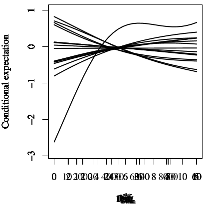
Figure 14: Plot of the conditional expectation of $\log[T^{(B)}_{8}(t=30)]$ given fixed values of $\tau_{E}$ for the DPM where we average over the uncertainty in the remaining model parameters.

Other parameters, such as the number of generations for the different subtypes, have a much more mundane effect, where the total number of antigen-specific cells increases as $g_{n}$, $g_{c}$ and $g_{m}$ increase. For $\lambda_{c}$, as this parameter increases, the total number of antigen-specific cells also increases. The same effect is observed for $\lambda_{n}$, $\lambda_{m}$ and $\phi$, whereas an opposite (but weaker effect) is seen for $\gamma$ (as shown in Figure 15).

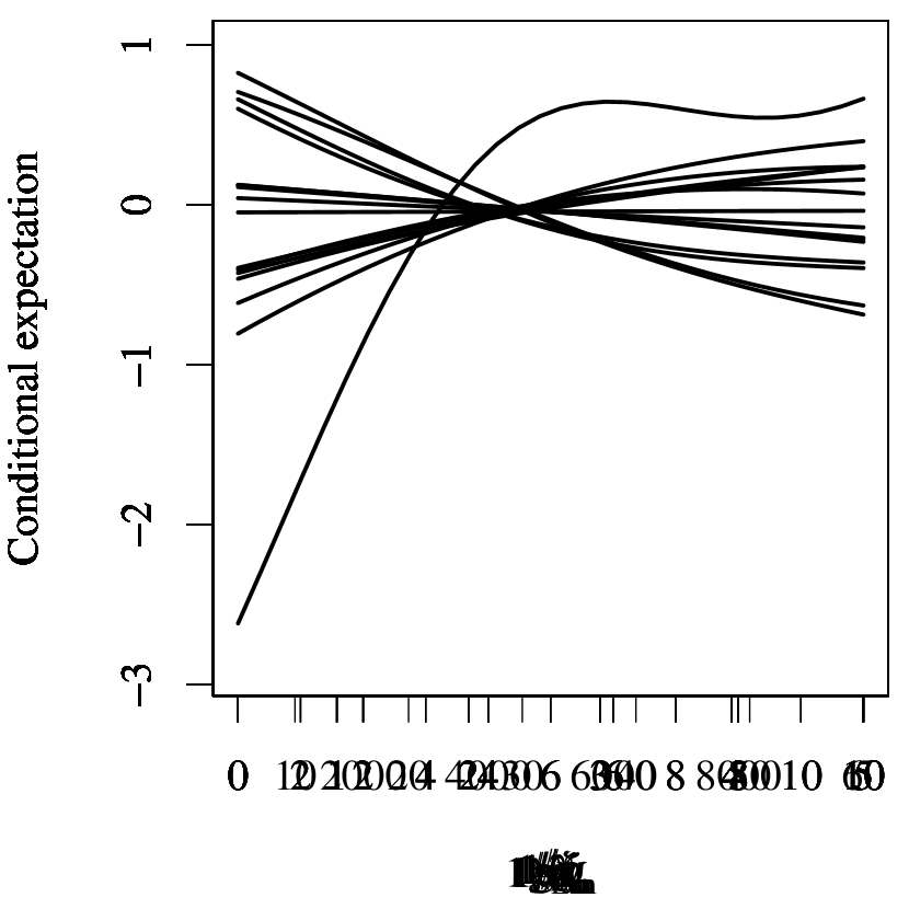
Figure 15: Plot of the conditional expectation of $\log[T^{(B)}_{8}(t=30)]$ given fixed values of four different input parameters in the DPM ($1/\lambda_{n}$, $1/\lambda_{c}$, $1/\phi$ and $1/\gamma$).

We also note that we may be able to rule out lower values of $N_{c}$ when we learn the parameters from data (see Section 3.1). This is because $N_{c}$ has an impact on the model outputs for low values alone. Essentially, the total number of CD8⁺ T cells is reduced for relatively small values of $N_{c}$, and this effect disappears for $N_{c}\gtrsim 25,000$, where the outputs are seemingly unaffected by $N_{c}$.

In addition to performing sensitivity analyses on the outputs that correspond to observed data, we can consider the influence of the input parameters on other model outputs, such as the maximum number of antigen-specific CD8⁺ T cells in blood and the time at which this maximum is realised. For the output $\max_{t}[T^{(B)}_{8}(t)]$, we found that $\tau_{E}$ and the number of generations had a leading role, alongside $\alpha_{m}$ and $\phi$. In fact, in order of relevance, the parameters that influence the output $\max_{t}[T^{(B)}_{8}(t)]$ are $\tau_{E},g_{c},g_{n},g_{m}$ and $\alpha_{m}$. It is clear from Figure 16 that, as the number of generations and $\tau_{E}$ increase, $\max_{t}[T^{(B)}_{8}(t)]$ increases.

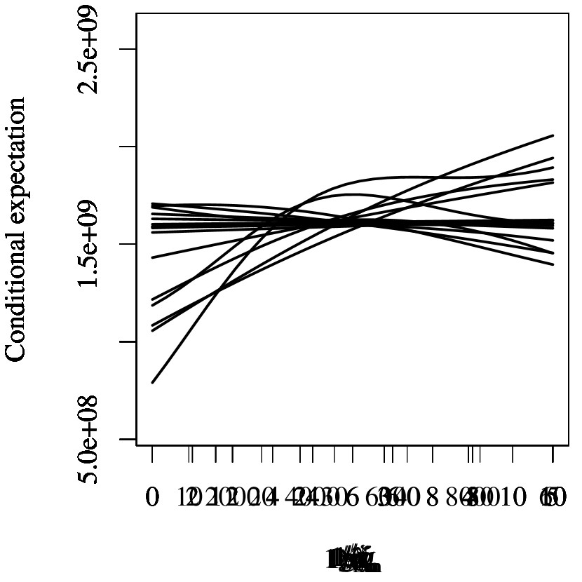
Figure 16: Plot of the conditional expectation for the maximum number of antigen-specific CD8⁺ T cells in blood given fixed values of four different input parameters in the DPM ($g_{n},g_{c},g_{m}$ and $\tau_{E}$ fixed one-at-a-time and averaging over the uncertainty in the remaining 15 parameters).

For the time at which $\max_{t}[T^{(B)}_{8}(t)]$ is realised, the most influential parameter by far is $\tau_{E}$ (the total effect of $\tau_{E}$ accounts for 85% of the variance in the time to the maximum). As expected, as $\tau_{E}$ increases, the time taken to reach the maximum increases (see Figure 17). For completeness, we also include a histogram for the time taken to reach the maximum in the DPM for $N_{c}^{max}=10^{5}$ (see Figure 18)

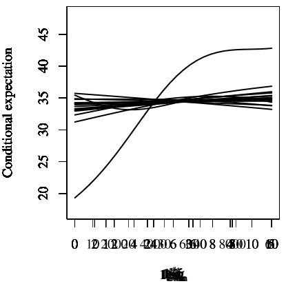
Figure 17: Plot of the conditional expectation for the time taken (in days) to reach the maximum number of antigen-specific CD8⁺ T cells in blood, $\max_{t}[T^{(B)}_{8}(t)]$, given fixed values of $\tau_{E}$ in the DPM.

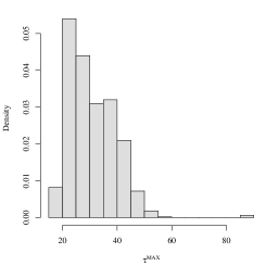
Figure 18: Histogram of the time taken to reach the maximum number of antigen-specific CD8⁺ T cells in blood, $\max_{t}[T^{(B)}_{8}(t)]$, based upon the posterior distributions of the DPM input parameters.

5.4.1 Sensitivity analysis for the increasing potential model: a brief comment

For completeness, we conducted the same probabilistic sensitivity analysis for the increasing potential model (both for individual outputs and for PCA transformed outputs). Four parameters are more influential than any others in that they regularly have relatively high total effect indices for all the outputs of interest: $\tau_{E}$, $g_{n}$, $\lambda_{n}$ and $g_{e}$. As in the case of the decreasing potential model, $\tau_{E}$ has a great impact on the number of antigen-specific cells in the blood compartment. There are several other input parameters that cause some of the variance for some of the outputs: $g_{c}$, $\alpha_{c}$, $\lambda_{e}$, $\lambda_{m}$, $\phi$ and $\xi$.

5.5 Calibration method

We take a Bayesian approach to the calibration of the simulator’s input parameters: we set prior distributions for each of the parameters and update them in the light of the data and the mathematical model. The updated distributions are called posterior distributions. Given the complexity of the model and the approximate nature of the likelihood, we employ an approximate Bayesian computation (ABC) approach [96]. For such an approach, we do not need to specify a likelihood function for the data given the simulator: we just need to be able to simulate data in a similar form to the data that we have. The basic ABC approach that we employ is as follows:

1. Decide on the number of required samples $N$, and set $i=0$.

2. Make a single draw from the prior distributions of the unknown input parameters.

3. Run the simulator in order to use the drawn input parameters to find a set of outputs that correspond to the data.

4. If the simulated data are sufficiently close to the observed data, add the drawn input parameters to your sample and increase $i$ by one.

5. If $i<N$, go to step 1.

In step 2, and to simulate data, we can run the simulator for any given set of input values to get a set of outputs that correspond to the data that we will observe. If we make the judgement that the simulator is providing outputs that correspond to the CD8⁺ specific T cell fraction $f_{8}(t)$ for the average human post-vaccination, then we need to also specify a mechanism that can generate the variability in the human population. For the specific T cell fraction at time $t$, $f_{8}(t)$, we use a log normal distribution with its mean provided by the simulator and a variance to be learnt from the data. These choices result in a need to learn the input parameters and the variability parameter value from the data. Given the data, plausible distributions are as follows:

$$\log\left(f_{8,\mbox{obs}}(t)\right)|\Theta,\sigma^{2}\sim\mbox{N}\left(f_{8,\mbox{model}}(t),\sigma^{2}\right)\leavevmode\nobreak\ \leavevmode\nobreak\ \leavevmode\nobreak\ \leavevmode\nobreak\ \mbox{for }t\in\{11,14,30,90\},$$

where $\Theta$ is the complete set of input parameters and $\sigma^{2}$ is the variance in the observed data.

In step 3, we compare the simulated data with the observed data. Here we must choose what distance measure to use and what tolerance is permitted. Both of these choices have an impact on the accuracy on the approximation. For instance, if we consider a Euclidean distance between the simulated and observed data sets and set the tolerance to be zero, then the algorithm provides an exact posterior result. In our case, because the data are continuous, there is zero chance of replicating the data exactly so we must have a non-zero tolerance and the size of the tolerance will determine the length of time it takes for the algorithm to produce the sample. We calculate the Euclidean distance between $\log\left[f_{8,\mbox{obs}}(t)\right]$ and $\log\left[f_{8,\mbox{model}}(t)\right]$ for each of the time points and for each of the individuals and compare this with tolerance $\epsilon_{T}$. The final value of $\epsilon_{T}$ we used was 13.5 for both the DPM and IPM models. Using the same value for the tolerance was important because the ABC results were used in the model comparison of Section 3.1.3.

References

- [1] Mahnke YD, Brodie TM, Sallusto F, Roederer M, Lugli E. The who’s who of T-cell differentiation: Human memory T-cell subsets. European Journal of Immunology. 2013;43(11):2797–2809.
- [2] Gattinoni L, Lugli E, Ji Y, Pos Z, Paulos CM, Quigley MF, et al. A human memory T cell subset with stem cell-like properties. Nature Medicine. 2011;17(10):1290–1297.
- [3] Lugli E, Dominguez MH, Gattinoni L, Chattopadhyay PK, Bolton DL, Song K, et al. Superior T memory stem cell persistence supports long-lived T cell memory. Journal of Clinical Investigation. 2013;123(2):0–0.
- [4] Kaech SM, Ahmed R. Memory CD8+ T cell differentiation: initial antigen encounter triggers a developmental program in naive cells. Nature Immunology. 2001;2(5):415–422.
- [5] Farber DL, Yudanin NA, Restifo NP. Human memory T cells: generation, compartmentalization and homeostasis. Nature Reviews Immunology. 2014;14(1):24–35.
- [6] Thome JJ, Yudanin N, Ohmura Y, Kubota M, Grinshpun B, Sathaliyawala T, et al. Spatial Map of Human T Cell Compartmentalization and Maintenance over Decades of Life. Cell. 2014;159(4):814–828.
- [7] Thome JJ, Bickham KL, Ohmura Y, Kubota M, Matsuoka N, Gordon C, et al. Early-life compartmentalization of human T cell differentiation and regulatory function in mucosal and lymphoid tissues. Nature Medicine. 2016;22(1):72–77.
- [8] Le D, Miller JD, Ganusov VV. Mathematical modeling provides kinetic details of the human immune response to vaccination. Frontiers in Cellular and Infection Microbiology. 2014;4.
- [9] De Boer RJ, Oprea M, Antia R, Murali-Krishna K, Ahmed R, Perelson AS. Recruitment times, proliferation, and apoptosis rates during the CD8+ T-cell response to lymphocytic choriomeningitis virus. Journal of Virology. 2001;75(22):10663–10669.
- [10] Althaus CL, Ganusov VV, De Boer RJ. Dynamics of CD8+ T cell responses during acute and chronic lymphocytic choriomeningitis virus infection. Journal of Immunology. 2007;179(5):2944–2951.
- [11] Akondy RS, Monson ND, Miller JD, Edupuganti S, Teuwen D, Wu H, et al. The yellow fever virus vaccine induces a broad and polyfunctional human memory CD8+ T cell response. Journal of Immunology. 2009;183(12):7919–7930.
- [12] Buchholz VR, Flossdorf M, Hensel I, Kretschmer L, Weissbrich B, Gräf P, et al. Disparate individual fates compose robust CD8+ T cell immunity. Science. 2013;340(6132):630–635.
- [13] Gerlach C, Rohr JC, Perié L, van Rooij N, van Heijst JW, Velds A, et al. Heterogeneous Differentiation Patterns of Individual CD8+ T Cells. Science. 2013;340(6132):635–639.
- [14] Gong C, Linderman JJ, Kirschner D. Harnessing the heterogeneity of T cell differentiation fate to fine-tune generation of effector and memory T cells. Frontiers in Immunology. 2014;5:57.
- [15] Thomas-Vaslin V, Altes HK, de Boer RJ, Klatzmann D. Comprehensive assessment and mathematical modeling of T cell population dynamics and homeostasis. Journal of Immunology. 2008;180(4):2240.
- [16] Appay V, Dunbar PR, Callan M, Klenerman P, Gillespie GM, Papagno L, et al. Memory CD8+ T cells vary in differentiation phenotype in different persistent virus infections. Nature medicine. 2002;8(4):379–385.
- [17] Gerritsen B, Pandit A. The memory of a killer T cell: models of CD8+ T cell differentiation. Immunology and cell biology. 2015;.
- [18] Schlub TE, Venturi V, Kedzierska K, Wellard C, Doherty PC, Turner SJ, et al. Division-linked differentiation can account for CD8+ T-cell phenotype in vivo. European Journal of Immunology. 2009;39(1):67–77.
- [19] Harty JT, Badovinac VP. Shaping and reshaping CD8+ T-cell memory. Nature Reviews Immunology. 2008;8(2):107–119.
- [20] Kaech SM, Cui W. Transcriptional control of effector and memory CD8+ T cell differentiation. Nature Reviews Immunology. 2012;12(11):749–761.
- [21] Gebhardt T, Mackay LK. Local immunity by tissue-resident CD8+ memory T cells. Frontiers in Immunology. 2012;3.
- [22] Antia R, Pilyugin SS, Ahmed R. Models of immune memory: on the role of cross-reactive stimulation, competition, and homeostasis in maintaining immune memory. Proceedings of the National Academy of Sciences. 1998;95(25):14926–14931.
- [23] Tanchot C, Lemonnier FA, Pérarnau B, Freitas AA, Rocha B. Differential requirements for survival and proliferation of CD8 naive or memory T cells. Science. 1997;276(5321):2057–2062.
- [24] Freitas AA, Rocha B. Population biology of lymphocytes: the flight for survival. Annual Review of Immunology. 2000;18(1):83–111.
- [25] Johnson PL, Goronzy JJ, Antia R. A population biological approach to understanding the maintenance and loss of the T-cell repertoire during aging. Immunology. 2014;142(2):167–175.
- [26] Takada K, Jameson SC. Naive T cell homeostasis: from awareness of space to a sense of place. Nature Reviews Immunology. 2009;9(12):823–832.
- [27] Boyman O, Létourneau S, Krieg C, Sprent J. Homeostatic proliferation and survival of naive and memory T cells. European Journal of Immunology. 2009;39(8):2088–2094.
- [28] Berard M, Tough DF. Qualitative differences between naive and memory T cells. Immunology. 2002;106(2):127–138.
- [29] Nolz JC, Starbeck-Miller GR, Harty JT. Naive, effector and memory CD8 T-cell trafficking: parallels and distinctions. Immunotherapy. 2011;3(10):1223–1233.
- [30] Masopust D, Vezys V, Marzo AL, Lefrançois L. Preferential localization of effector memory cells in nonlymphoid tissue. Science. 2001;291(5512):2413–2417.
- [31] Mueller SN, Gebhardt T, Carbone FR, Heath WR. Memory T cell subsets, migration patterns, and tissue residence. Annual Review of Immunology. 2013;31:137–161.
- [32] Benechet AP, Menon M, Khanna KM. Visualizing T Cell Migration in situ. Frontiers in Immunology. 2014;5.
- [33] Ahmed R, Bevan MJ, Reiner SL, Fearon DT. The precursors of memory: models and controversies. Nature Reviews Immunology. 2009;9(9):662–668.
- [34] Zhu J, Adli M, Zou JY, Verstappen G, Coyne M, Zhang X, et al. Genome-wide chromatin state transitions associated with developmental and environmental cues. Cell. 2013;152(3):642–654.
- [35] Sukumar M, Liu J, Ji Y, Subramanian M, Crompton JG, Yu Z, et al. Inhibiting glycolytic metabolism enhances CD8+ T cell memory and antitumor function. Journal of Clinical Investigation. 2013;123(10):4479–4488.
- [36] Restifo NP, Gattinoni L. Lineage relationship of effector and memory T cells. Current Opinion in Immunology. 2013;25(5):556–563.
- [37] Ahmed R, Gray D. Immunological memory and protective immunity: understanding their relation. Science. 1996;272(5258):54–60.
- [38] Lanzavecchia A, Sallusto F. Progressive differentiation and selection of the fittest in the immune response. Nature Reviews Immunology. 2002;2(12):982–987.
- [39] Huster KM, Koffler M, Stemberger C, Schiemann M, Wagner H, Busch DH. Unidirectional development of CD8+ central memory T cells into protective Listeria-specific effector memory T cells. European Journal of Immunology. 2006;36(6):1453–1464.
- [40] Joshi NS, Cui W, Chandele A, Lee HK, Urso DR, Hagman J, et al. Inflammation Directs Memory Precursor and Short-Lived Effector CD8+ T Cell Fates via the Graded Expression of T-bet Transcription Factor. Immunity. 2007;27(2):281–295.
- [41] Buchholz VR, Gräf P, Busch DH. The origin of diversity: studying the evolution of multi-faceted CD8+ T cell responses. Cellular and Molecular Life Sciences. 2012;p. 1–11.
- [42] Cieri N, Camisa B, Cocchiarella F, Forcato M, Oliveira G, Provasi E, et al. IL-7 and IL-15 instruct the generation of human memory stem T cells from naive precursors. Blood. 2013;121(4):573–584.
- [43] Hodgkin PD, Lee JH, Lyons AB. B cell differentiation and isotype switching is related to division cycle number. Journal of Experimental Medicine. 1996;184(1):277–281.
- [44] Gett AV, Hodgkin PD. Cell division regulates the T cell cytokine repertoire, revealing a mechanism underlying immune class regulation. Proceedings of the National Academy of Sciences. 1998;95(16):9488–9493.
- [45] Hogan T, Shuvaev A, Commenges D, Yates A, Callard R, Thiebaut R, et al. Clonally Diverse T Cell Homeostasis Is Maintained by a Common Program of Cell-Cycle Control. Journal of Immunology. 2013;190(8):3985–3993.
- [46] Marchingo JM, Kan A, Sutherland RM, Duffy KR, Wellard CJ, Belz GT, et al. Antigen affinity, costimulation, and cytokine inputs sum linearly to amplify T cell expansion. Science. 2014;346(6213):1123–1127.
- [47] Hasbold J, Gett A, Rush J, Deenick E, Avery D, Jun J, et al. Quantitative analysis of lymphocyte differentiation and proliferation in vitro using carboxyfluorescein diacetate succinimidyl ester. Immunology and Cell Biology. 1999;77(6):516–522.
- [48] Moon JJ, Chu HH, Pepper M, McSorley SJ, Jameson SC, Kedl RM, et al. Naive CD4+ T Cell Frequency Varies for Different Epitopes and Predicts Repertoire Diversity and Response Magnitude. Immunity. 2007;27(2):203–213.
- [49] Obar JJ, Khanna KM, Lefrançois L. Endogenous naive CD8+ T cell precursor frequency regulates primary and memory responses to infection. Immunity. 2008;28(6):859–869.
- [50] Pewe LL, Netland JM, Heard SB, Perlman S. Very diverse CD8 T cell clonotypic responses after virus infections. Journal of Immunology. 2004;172(5):3151–3156.
- [51] Ahmed R, Akondy RS. Insights into human CD8+; T-cell memory using the yellow fever and smallpox vaccines. Immunology and Cell Biology. 2011;89(3):340–345.
- [52] Antia R, Bergstrom CT, Pilyugin SS, Kaech SM, Ahmed R. Models of CD8+ responses: 1. What is the antigen-independent proliferation program. Journal of Theoretical Biology. 2003;221(4):585–598.
- [53] Craig PS, Goldstein M, Seheult A, Smith J. Constructing partial prior specifications for models of complex physical systems. Journal of the Royal Statistical Society: Series D (The Statistician). 1998;47(1):37–53.
- [54] O’Hagan A, Buck CE, Daneshkhah A, Eiser JE, Garthwaite PH, Jenkinson D, et al. Uncertain judgements: eliciting expert probabilities. Chichester: Wiley; 2006.
- [55] Saltelli A, Chan K, Scott EM, editors. Sensitivity Analysis. New York: Wiley; 2000.
- [56] Oakley JE, O’Hagan A. Probabilistic sensitivity analysis of complex models: a Bayesian approach. Journal of the Royal Statistical Society: Series B (Statistical Methodology). 2004;66(3):751–769.
- [57] Sobol IM. Global sensitivity indices for nonlinear mathematical models and their Monte Carlo estimates. Mathematics and Computers in Simulation. 2001;55(1):271–280.
- [58] Gelman A, Bois F, Jiang J. Physiological pharmacokinetic analysis using population modeling and informative prior distributions. Journal of the American Statistical Association. 1996;91(436):1400–1412.
- [59] Girolami M. Bayesian inference for differential equations. Theoretical Computer Science. 2008;408(1):4–16.
- [60] Robey, Chu, Gosling, Lythe, Molina-París. Continuous effector T cell production by an amplifying intermediate in a controlled persistent infection. Immunity. 2016;.
- [61] Obar JJ, Jellison ER, Sheridan BS, Blair DA, Pham QM, Zickovich JM, et al. Pathogen-induced inflammatory environment controls effector and memory CD8+ T cell differentiation. Journal of Immunology. 2011;187(10):4967–4978.
- [62] Wherry EJ, Teichgräber V, Becker TC, Masopust D, Kaech SM, Antia R, et al. Lineage relationship and protective immunity of memory CD8 T cell subsets. Nature Immunology. 2003;4(3):225–234.
- [63] Chipman H, George EI, McCulloch RE, Clyde M, Foster DP, Stine RA. The practical implementation of Bayesian model selection. Lecture Notes-Monograph Series. 2001;p. 65–134.
- [64] Gett AV, Sallusto F, Lanzavecchia A, Geginat J. T cell fitness determined by signal strength. Nature Immunology. 2003;4(4):355–360.
- [65] Yan AW, Cao P, Heffernan JM, McVernon J, Quinn KM, La Gruta NL, et al. Modelling cross-reactivity and memory in the cellular adaptive immune response to influenza infection in the host. Journal of Theoretical Biology. 2017;413:34–49.
- [66] Martin SF, Esser PR, Weber FC, Jakob T, Freudenberg MA, Schmidt M, et al. Mechanisms of chemical-induced innate immunity in allergic contact dermatitis. Allergy. 2011 sep;66(9):1152–63. Available from: http://www.ncbi.nlm.nih.gov/pubmed/21599706.
- [67] Popple A, Williams J, Maxwell G, Gellatly N, Dearman RJ, Kimber I. T lymphocyte dynamics in methylisothiazolinone-allergic patients. Contact Dermatitis. 2016 jul;75(1):1–13. Available from: http://www.ncbi.nlm.nih.gov/pubmed/27145152.
- [68] Oakes T, Popple A, Williams J, Best K, Heather JM, Ismail M, et al. The T cell response to the contact sensitiser paraphenylenediamine is characterised by a polyclonal diverse repertoire of antigen specific receptors. Submitted to: Journal of Allergy and Clinical Immunology. 2016;.
- [69] Kaech SM, Wherry EJ, Ahmed R. Effector and memory T-cell differentiation: implications for vaccine development. Nature Reviews Immunology. 2002;2(4):251–262.
- [70] Arstila TP, Casrouge A, Baron V, Even J, Kanellopoulos J, Kourilsky P. A direct estimate of the human T cell receptor diversity. Science. 1999;286(5441):958–961.
- [71] Ganusov VV, De Boer RJ. Do most lymphocytes in humans really reside in the gut? Trends in Immunology. 2007;28(12):514–518.
- [72] Westermann J, Pabst R. Distribution of lymphocyte subsets and natural killer cells in the human body. The Clinical Investigator. 1992;70(7):539–544.
- [73] Vrisekoop N, den Braber I, de Boer AB, Ruiter AF, Ackermans MT, van der Crabben SN, et al. Sparse production but preferential incorporation of recently produced naive T cells in the human peripheral pool. Proceedings of the National Academy of Sciences. 2008;105(16):6115–6120.
- [74] Sathaliyawala T, Kubota M, Yudanin N, Turner D, Camp P, Thome JJ, et al. Distribution and compartmentalization of human circulating and tissue-resident memory T cell subsets. Immunity. 2013;38(1):187–197.
- [75] Westera L, Hoeven V, Drylewicz J, Spierenburg G, Velzen JF, Boer RJ, et al. Lymphocyte maintenance during healthy aging requires no substantial alterations in cellular turnover. Aging Cell. 2015;14(2):219–227.
- [76] Goroll AH, Mulley AG. Primary care medicine: office evaluation and management of the adult patient. Lippincott Williams & Wilkins; 2012.
- [77] Susan S. Greys Anatomy 40th edition Churchill Livingstone. Spain 2008. 2008;9.
- [78] Pabst R. Plasticity and heterogeneity of lymphoid organs: what are the criteria to call a lymphoid organ primary, secondary or tertiary? Immunology Letters. 2007;112(1):1–8.
- [79] O’Rahilly R, Swenson R, Muller F, Carpenter S, Catlin B, et al. Basic human anatomy. Philadelphia: WB Saunders. 1983;162.
- [80] Qi Q, Liu Y, Cheng Y, Glanville J, Zhang D, Lee JY, et al. Diversity and clonal selection in the human T-cell repertoire. Proceedings of the National Academy of Sciences. 2014;111(36):13139–13144.
- [81] Chamuleau ME, Westers TM, van Dreunen L, Groenland J, Zevenbergen A, Eeltink CM, et al. Immune mediated autologous cytotoxicity against hematopoietic precursor cells in patients with myelodysplastic syndrome. Haematologica. 2009;94(4):496–506.
- [82] Riddell NE, Griffiths SJ, Rivino L, King DC, Teo GH, Henson SM, et al. Multifunctional cytomegalovirus (CMV)-specific CD8+ T cells are not restricted by telomere-related senescence in young or old adults. Immunology. 2015;144(4):549–560.
- [83] Roos MTL, van Lier RA, Hamann D, Knol GJ, Verhoofstad I, van Baarle D, et al. Changes in the composition of circulating CD8+ T cell subsets during acute Epstein-Barr and human immunodeficiency virus infections in humans. Journal of Infectious Diseases. 2000;182(2):451–458.
- [84] Hong MS, Dan JM, Choi JY, Kang I. Age-associated changes in the frequency of naive, memory and effector CD8+ T cells. Mechanisms of Ageing and Development. 2004;125(9):615–618.
- [85] Saule P, Trauet J, Dutriez V, Lekeux V, Dessaint JP, Labalette M. Accumulation of memory T cells from childhood to old age: central and effector memory cells in CD4+ versus effector memory and terminally differentiated memory cells in CD8+ compartment. Mechanisms of Ageing and Development. 2006;127(3):274–281.
- [86] Murray JM, Kaufmann GR, Hodgkin PD, Lewin SR, Kelleher AD, Davenport MP, et al. Naive T cells are maintained by thymic output in early ages but by proliferation without phenotypic change after age twenty. Immunology and Cell Biology. 2003;81(6):487–495.
- [87] den Braber I, Mugwagwa T, Vrisekoop N, Westera L, Mögling R, de Boer AB, et al. Maintenance of peripheral naive T cells is sustained by thymus output in mice but not humans. Immunity. 2012;36(2):288–297.
- [88] Mclean AR, Michie CA. In vivo estimates of division and death rates of human T lymphocytes. Proceedings of the National Academy of Sciences. 1995;92(9):3707–3711.
- [89] Ganusov VV, Auerbach J. Mathematical modeling reveals kinetics of lymphocyte recirculation in the whole organism. PLoS Computational Biology. 2014;p. e1003586.
- [90] Mandl JN, Liou R, Klauschen F, Vrisekoop N, Monteiro JP, Yates AJ, et al. Quantification of lymph node transit times reveals differences in antigen surveillance strategies of naive CD4+ and CD8+ T cells. Proceedings of the National Academy of Sciences. 2012;109(44):18036–18041.
- [91] Schwab SR, Cyster JG. Finding a way out: lymphocyte egress from lymphoid organs. Nature Immunology. 2007;8(12):1295–1301.
- [92] Seabrook TJ, Borron PJ, Dudler L, Hay JB, Young AJ. A novel mechanism of immune regulation: interferon- regulates retention of CD4+ T cells during delayed type hypersensitivity. Immunology. 2005;116(2):184–192.
- [93] Miller JD, van der Most RG, Akondy RS, Glidewell JT, Albott S, Masopust D, et al. Human Effector and Memory CD8+ T Cell Responses to Smallpox and Yellow Fever Vaccines. Immunity. 2008;28(5):710–722.
- [94] Hommel M, Hodgkin PD. TCR affinity promotes CD8+ T cell expansion by regulating survival. Journal of Immunology. 2007;179(4):2250–2260.
- [95] Becattini S, Latorre D, Mele F, Foglierini M, De Gregorio C, Cassotta A, et al. Functional heterogeneity of human memory CD4+ T cell clones primed by pathogens or vaccines. Science. 2015;347(6220):400–406.
- [96] Marin JM, Pudlo P, Robert CP, Ryder RJ. Approximate Bayesian computational methods. Statistics and Computing. 2012;22(6):1167–1180.