A Study of the Abundance of Low-Z Elements in
the Sun During its Whole Predicted Life

Abstract

The study of the elemental composition of stars and galaxies is a key topic for understanding their origin and evolution. In this study, we present the results of the calculation of solar abundances of the isotopes ¹H, ⁴He, ¹²C, ¹⁴N, ¹⁵O, ¹⁶O, ¹⁷O, and ¹⁸O during the four phases of the solar life; Hydrogen burning, Onset of rapid growth and red giant, Helium burning and Helium exhaustion. The open source package nucnet-tools from the Webnucleo Group in Clemson University, SC, USA was used for this purpose. The results for all isotopes are listed in tables for future use. Abundances found, globally, agree fairly well with those predicted in the literature. Results obtained for the last two phases have no equivalent elsewhere.

I Introduction

The theory of stellar evolution is by now well established, after more than sixty years of continuous development, and its main predictions confirmed by various empirical tests (Salaris & Cassisi, 2006). Thanks to the works of Bethe (Bethe, 1939), (Burbidge et al., 1957), and many others, the study of the elemental composition of stars and galaxies, revealed to be a key topic for understanding the origin and evolution of these remote objects (Gargaud et al., 2011),(Wallerstein et al., 1997). Tools for understanding the stellar evolution are 1) atomic spectroscopy, which allows the determination of the elemental abundances in stars, interstellar gas, and galaxies, and 2) nuclear mass spectroscopy, which is used for precise determination of most isotope abundances in Earth, lunar, and meteoritic samples. The abundance of a given element is the relative amount (or fraction) of this element in a sample of matter. It can be expressed either: - in relative terms with respect to the amount of some key element, e.g., the most abundant one, in the sample. - in absolute terms (definition adopted in this work), i.e., with respect to the total amount of matter in the sample. The abundance is expressed in terms of mass fractions; i.e. the mass fraction of a given nuclide to the total mass of the star. Measurements of oxygen abundances in stars or in presolar grains of different ages provide important clues about the chemical evolution of the Galaxy (Meyer et al., 2008). The isotopes of oxygen are a crucial diagnostic tool of nucleosynthesis and Galactic chemical evolution. This is due in large part to oxygen’s high abundance. ¹⁶O is the third most abundant element in the solar system, though considerably less abundant than hydrogen and helium (principally produced in primordial nucleosynthesis). According to the compilation of Lodders (Lodders, 2003) oxygen’s abundance is nearly equal to that of all the other heavy elements (elements with atomic number greater than that of helium) combined (Yurimoto et al., 2007).

Despite the low relative abundances of ¹⁷O and ¹⁸O, they are still sufficiently abundant that they can be measured in stellar atmospheres. Oxygen isotopic abundances are also readily measured in presolar grains in meteorites and interplanetary dust particles. These measurements provide key constraints on nucleosynthesis and stellar evolution (Lodders et al., 2009). The fact that its three stable isotopes are predominantly made in different burning epochs during the life of a star, contributes to oxygen’s importance as a diagnostic tool. ¹⁷O is predominantly made in hydrogen burning, ¹⁸O is predominantly made in the early stages of helium burning and ¹⁶O is made in the later part of helium burning. Thus, the isotopic composition of a stellar atmosphere or a presolar grain provides clues to the stellar region in which the major part of the material was synthesized (El Eid et al., 2004).

Finally, a third significant aspect of oxygen’s role, as a diagnostic tool of nucleosynthesis and galactic chemical evolution, is the primary versus secondary nature of the different isotopes. ¹⁶O is a primary isotope, that is, an isotope that can be synthesized in a star initially composed only of hydrogen, while ¹⁷O and ¹⁸O are secondary isotopes, which means that their formation requires pre-existing seed nuclei from previous stellar generations (Meyer et al., 2008). As a consequence, the abundance of ¹⁶O relative to those of ¹⁷O and ¹⁸O changes with time in the Galaxy’s history. 4.56 billion years ago, our sun started to burn hydrogen and entered the main sequence phase. It will continue in this phase for at least 6.34 billion years until the hydrogen runs out http://www.astronomy.ohio-state.edu/ pogge/. In this paper we present the theoretical calculations of the abundances of the following isotopes: ¹H, ⁴He, ¹²C, ¹⁴N, ¹⁵O, ¹⁶O, ¹⁷O, and ¹⁸O; over the ”whole lifetime” of the sun, i.e. the four phases: Hydrogen burning, Old age, Rapid Growth and Red Giant, Helium burning, and Helium Exhaustion http://www.astronomy.ohio-state.edu/ pogge/. To our knowledge, except (Talafha, 2016).

II Methodology

II.1 Calculating the abundance

In order to calculate the abundance of a given element; one, first, has to define the series of reactions (network) leading to its production and destruction. This leads to a system of coupled differential equations, known as Bateman equations (Krane & Lynch, 1989). These equations are, generally, solved numerically using specific temperature and density as initial conditions. The open-source package nucnet-tools, initiated and developed by the Webnucleo project headed by Bradley S. Meyer, Astronomy and Astrophysics group at Clemson University, South Carolina, USA https://sourceforge.net/p/libnucnet/home/Home/, was used for this purpose. In addition, nucnet-tools allows the determination of the abundance of elements in stars. The sun is being taken as an example in many of the scripts composing the package (Meyer, 2012). In this work, calculation of the abundance of low-Z elements, namely ¹H, ⁴He, ¹²C, ¹⁴N and the oxygen isotopes ¹⁵O, ¹⁶O, ¹⁷O, and ¹⁸O, in the core of the sun is achieved using ”nucnet tools”. A series of scripts is used in order to calculate the network leading to the production and destruction of an isotope. The Newton-Raphson Method is used for solving the system of equations required for the calculation of the abundance of the isotope, in an iterated method until a defined convergence is reached. The procedure is detailed and well explained in (Meyer, 2012).
As mentioned above, the temperature and density are the main parameters for initializing the calculation. They both, mainly, depend on the expansion timescale ($\tau$) which can be defined as (Meyer, 2012):

$$\frac{1}{\tau}=-\frac{1}{\rho_{\circ}}\frac{\partial\rho}{\partial t}$$ (1)

So that the density changes as:

$$\rho(t)=\rho_{\circ}exp(-t/\tau)$$ (2)

and the temperature T₉ = T/10⁹ K is such that $\rho\propto T^{3}_{9}$(Meyer, 2012).

Here, the expansion time scale,$\tau$, is taken equal to infinity. This choice means that the temperature T and density ($\rho$), in the center of the sun, remain constants with time. The initial values of T and $\rho$ are, respectively, 1.548 $\times$ 10⁷ K, 1.505 $\times$ 10² g/cm³ at time t = 10.9 billion years.

Appropriate nuclides and reactions data from the JINA (Joint Institute for Nuclear Astrophysics) database  (Côté et al., 2017) are used when needed.

II.2 Production and destruction of oxygen isotopes

The following reactions contribute to the production of oxygen isotopes (Meyer et al., 2008): ${}^{14}_{7}N$(p,$\gamma$)${}^{15}_{8}O$, ${}^{19}_{9}F$(p,$\alpha$)${}^{16}_{8}O$, ${}^{15}_{7}N$(p,$\gamma$)${}^{16}_{8}O$, ${}^{12}_{6}C$($\alpha$,$\gamma$)${}^{16}_{8}O$, and the two decay reactions: ${}^{17}_{9}F\longrightarrow^{17}_{8}O+e^{+}+v_{e}$ and ${}^{18}_{9}F\longrightarrow^{18}_{8}O+e^{+}+v_{e}$.

The decay reaction, always has constant reaction rates. ”nucnet-tools” allows the calculation of such reaction rates.We find, for example, that the reactions ${}^{17}_{9}F\longrightarrow^{17}_{8}O+e^{+}+v_{e}$ and ${}^{18}_{9}F\longrightarrow^{18}_{8}O+e^{+}+v_{e}$ have the rates 1.0746$\times$10^-2 and 1.0518$\times$10^-4 respectively.

It is worth noting that the reactions rates in the output are the product N_A $\left<v\right>$ which has units of cm³ mole^-1 s^-1,where N_A is the Avogadro’s number, is the reaction’s cross-section and v is the velocity of the projectile. The destruction of oxygen isotopes occurs by several reactions, such as: ${}^{16}_{8}O$(p,$\gamma$)${}^{17}_{9}F$, ${}^{17}_{8}O$(p,$\gamma$)${}^{18}_{9}F$, ${}^{17}_{8}O$(p,$\alpha$)${}^{14}_{7}N$, ${}^{18}_{8}O$(p,$\gamma$)${}^{19}_{9}F$, and ${}^{15}_{8}O\longrightarrow^{15}_{7}N+e^{+}+v_{e}$. Some of these reactions involve a proton or an alpha giving a new heavier element, and some of them are decay reactions which have a constant reaction rate at any temperature such as ${}^{15}_{8}O\longrightarrow^{15}_{7}N+e^{+}+v_{e}$ with rate 5.6816$\times$10^-3.

III Results

Calculations were performed over the ”whole lifetime” of the sun. The first two columns in Table 1 show the consecutive phases of our sun and their lifetimes, as in http://www.astronomy.ohio-state.edu/ pogge/. The initial values of the important parameters for achieving the iterations, namely; the temperature (10⁹ K), density (g/cm³), and the value of abundance to start with, are also shown in Table  1.

Preliminary note: the figures herein illustrate the most significant results. The initial values for the abundance of the studied isotopes are shown in Table 2. All results are compiled in a single table (Table 3).

Calculations are run with an infinite expansion timescale ($\tau$). In addition the initial conditions in Table 2 are assumed. The electron screening and nuclear statistical corrections are neglected in these calculations. The radius of the sun changes during phases, so that, the density changes accordingly. The density in phases II, III, and IV are taken to be $\rho$ = $\rho_{\circ}\times r^{3}$, where r is the radius of the sun (in units of the actual radius, R_∘) at the beginning of each phase http://www.astronomy.ohio-state.edu/ pogge/

Table 1: Phases of the Sun. Initial conditions for each phase in the sun’s lifetime.

Phase	Duration	Temp.(109 K)	Density(g/cm3)	Abundance
Hydrogen Burning	10.9 Gy	0.0154	$\rho_{0}$ = 150.5	Lodders
Old age,	1301 My	0.0154	$\rho$ = $\rho_{0}\times(2.3)^{3}$ = 1831.1335	last step in H burning
Rapid Growth and RG
Helium Burning	110 My	0.1	$\rho$ = $\rho_{0}\times(9.5)^{3}$ = 129034.9375	last step in previous phase
Helium Exhaustion	20 My	0.6	$\rho$ = $\rho_{0}\times(18)^{3}$ =877716	last step in He burning
	12.331 Gy

Table 2: Initial values (t = 0) of the abundance of the studied elements from (Lodders, 2003)

	1H	4He	12C	14N	15O	16O	17O	18O
Initial values (t = 0)	0.7109	0.2741	0.0025	0.0008	1.18$\times 10^{-25}$	0.0066	2.62$\times 10^{-6}$	1.49$\times 10^{-5}$

III.1 Phase I: The H Burning Phase

Hydrogen burning is the first phase in the lifetime of the sun, where hydrogen burns to produce helium, it will continue for 10.9 Gy. Figures 1 to 5 show, the mass fractions of the isotopes ¹H with ⁴He, ¹²C, ¹⁴N and the oxygen isotopes ¹⁶O, ¹⁷O and ¹⁸O, respectively, during this phase. One can see from these figures, that for the last time step in the calculation (10.9 Gy), the abundance for ¹H is X = 0.1121, for ⁴He is Y = 0.8725 and is 6.86$\times$10^-6 for ¹²C. These results together with the abundances for ¹⁴N and the oxygen isotopes (¹⁵O, ¹⁶O, ¹⁷O and ¹⁸O) are shown in Table 3.

III.2 Phase II: Old age, Onset rapid growth, and red giant (1.301 Gy)

After the hydrogen core is exhausted, the helium atoms become unstable and start to collapse under their own weight which makes the core hotter and denser while the remaining hydrogen gets moved out into a thin shell surrounding the helium core. The next 700 My (phase ending at 11.6 Gy) show a slow evolution where the brightness remains constant and the radius gets bigger; the sun becomes a subgiant star. After that, the subgiant Sun starts a rapid growth in size for 601 My (after 12.201 Gy from its birth). At that time, the stellar wind begins and the outer parts of the sun’s envelope get lost to the wind. The red giant phase starts at 12.233 Gy, the sun becomes brighter and bigger to engulf Mercury, the helium core will reach a temperature of 100 Million degrees and helium fusion ignites in the core producing carbon and oxygen http://www.astronomy.ohio-state.edu/ pogge/. Calculations show no significant variation of the mass fraction of all the studied elements over the total period of 1301 My. Thus the two previous periods were grouped in one phase (phase II of 1.301 Gy). Calculations show that for the last time step (1301 My) the abundance for ¹H is X = 1.62 $\times$10^-13, for ⁴He is Y = 0.8736. The corresponding abundance of ¹² C is 6.87 $\times$ 10^-6. These results together with the abundances for ¹⁴N and the oxygen isotopes (¹⁵O, ¹⁶O, ¹⁷O, and ¹⁸O) are shown in Table 3.
As expected, the star runs out of hydrogen and the main source of energy is the helium burning.

III.3 Phase III: Helium Burning Phase

At 12.201 Gy the red giant settles down for a 110 My of stability as a helium burning star. At the end of this period, the giant’s core finally runs out of helium and the C-O ash begins to collapse rapidly http://www.astronomy.ohio-state.edu/ pogge/. Table 3 shows the mass fractions of the studied elements during this phase.

III.4 Phase IV: Helium Exhaustion Phase

Finally, and the calculations stop here, the same procedure is used for the He exhaustion phase which lasts for 20 My. The mass fractions of all the studied elements during the helium exhaustion phase are shown and discussed in Table 3. At the last time step of the helium exhaustion phase the abundance of elements will be X = 8.22782 $\times$10^-34 for ¹H, Y = 3.469325$\times$10^-20 for ⁴He and 2.20796 $\times$10^-14 for ¹²C. Calculations were also done for ¹⁹O, following the same procedure as for the other isotopes. The calculations give infinitesimally small mass fractions for all the four phases. For simplicity and clarity, the choice was made to add the discussion of this work’s results as part of Table 3.

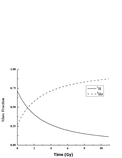
(a) Abundance of ¹H and ⁴He in the H-burning phase

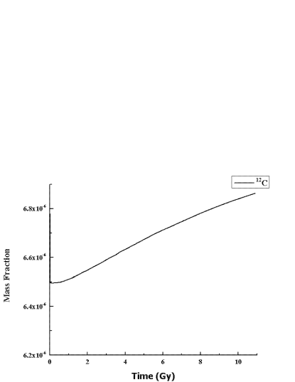
(b) Abundance of ¹²C in the H-burning phase

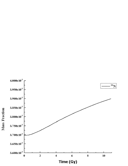
(c) Abundance of ¹⁴N in the H-burning phase

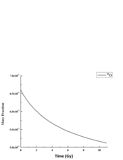
(d) Abundance of ¹⁶O in the H-burning phase

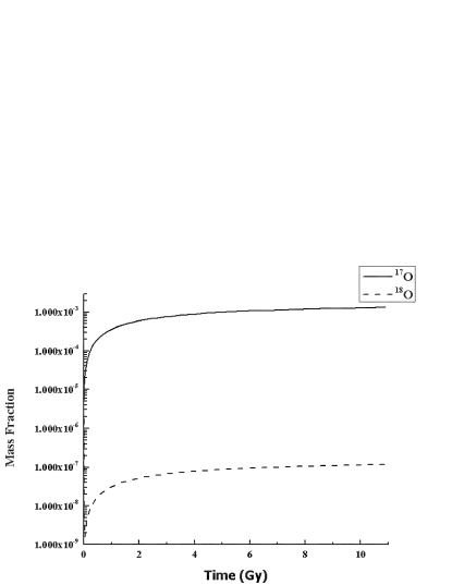
(e) Abundance of ¹⁷O and ¹⁸O in the H-burning phase

Figure 1: Abundances of Low-z elements during the five phases of the sun.

IV Conclusions

In this work, the abundance of the isotopes ¹H, ⁴He, ¹²C, ¹⁴N, ¹⁵O, ¹⁶O, ¹⁷O, and ¹⁸O in the core of our sun, were calculated over a period of 12.331 Gy. The main tool used is the open source package nucnet-tools from the Webnucleo Group in Clemson University, South Carolina, USA. The predicted lifetime of the sun is divided into four main phases; namely 1) Hydrogen burning, 2) Lively old age, Onset rapid growth and red giant, 3) Helium burning and 4) Helium exhaustion (Table 1). The initial abundances of the elements were taken from Lodders compilation for proto-sun. The obtained results, in this work, confirm the predictions by nuclear physics models. To avoid redundancy, the reader is referred to the last column in Table 3 which resumes all the conclusions that can be driven from this work. But globally, one can say that the calculations are consistent with the theoretical predictions of the abundance of studied isotopes, and especially the oxygen isotopes, in the core of the sun.

Table 3: Abundance of the studied elements at the end of each of the 4 phases and major observations

Element	Phase	Abundance
	I	0.1121	Mass fraction decreases in phases I, II. At the end of phase IV
${}^{1}H$	II	0.0441804	there is almost no hydrogen.
	III	1.23$\times 10^{-25}$
	IV	1.99$\times 10^{-26}$
	I	0.8725	The mass fraction of 4He increases and reaches a maximum at
${}^{4}He$	II	0.940427	the end of phase III. 20 My after that, i.e. at the end of the
	III	0.3187	last phase (IV) starts,the so-called, Helium flash. This phase
	IV	8.78$\times 10^{-18}$	is beyond our study.
	I	6.86$\times 10^{-6}$	The mass fraction of 12C increases very slowly and reaches
${}^{12}C$	II	6.9$\times 10^{-6}$	a maximum at the end of phase III. In the last phase (IV)
	III	0.3893	12C is still present in a fraction much larger than that of 1H.
	IV	0.00198
	I	0.0039	The mass fraction of 14N is almost stable over the first
${}^{14}N$	II	0.004	two phases (12.201 Gy) then it increases and reaches
	III	8.37$\times 10^{-3}$	a maximum at the end of phase III. In the last phase
	IV	5.49$\times 10^{-11}$	(IV) 14N almost vanishes.
	I	1.60$\times 10^{-17}$	The mass fraction of 15O is almost stable over the four phases.
${}^{15}O$	II	7.10$\times 10^{-17}$	It constantly decreases to a very small fraction. This is expected
	III	1.72$\times 10^{-26}$	since this isotope is unstable (half-life = 122 s)
	IV	Less than 1$\times 10^{-30}$
	I	5.10$\times 10^{-3}$	The mass fraction of 16O is almost stable till the end of phase III.
${}^{16}O$	II	4.81$\times 10^{-3}$	In the last 20 My, a drastic decrease is found. Nevertheless,
	III	0.2775	this isotope is still present at the end of the four phases.
	IV	0.030
	I	0.0013	The mass fraction of 17O is almost stable till the end of phase II.
${}^{17}O$	II	0.0015	This stable isotope is still present at the end of the first three
	III	1.08$\times 10^{-9}$	phases. Nevertheless a drastic decrease is found in the last phase,
	IV	1.20$\times 10^{-9}$	as expected.
	I	1.17$\times 10^{-7}$	The mass fraction of 17O is very small compared to 16O. Its
${}^{18}O$	II	1.33$\times 10^{-7}$	abundance is larger in the first two phases, as mentioned in
	III	7.80$\times 10^{-4}$	the text. The obvious variations from phase to another is due
	IV	2.55$\times 10^{-11}$	to the reactions of its production and destruction. A clarification
			can be obtained thanks to a future study on the calculation of
			reaction rates of the oxygen isotopes
${}^{19}O$	all phases	Infinitesimal traces

References

- Bethe (1939) Bethe H. A., 1939, Physical Review, 55, 103
- Burbidge et al. (1957) Burbidge E. M., Burbidge G. R., Fowler W. A., Hoyle F., 1957, Reviews of Modern Physics, 29, 547
- Côté et al. (2017) Côté B., Ritter C., Herwig F., O’Shea B. W., Pignatari M., Silvia D., Jones S., Fryer C. L., 2017, in Kubono S., Kajino T., Nishimura S., Isobe T., Nagataki S., Shima T., Takeda Y., eds, 14th International Symposium on Nuclei in the Cosmos (NIC2016) JINA-NuGrid Galactic Chemical Evolution Pipeline. p. 020203
- El Eid et al. (2004) El Eid M. F., Meyer B. S., The L.-S., 2004, Astrophys. J. , 611, 452
- Gargaud et al. (2011) Gargaud M., Amils R., Quintanilla J. C., Cleaves H. J. ., Irvine W. M., Pinti D. L., Viso M., 2011, Encyclopedia of Astrobiology
- Krane & Lynch (1989) Krane K. S., Lynch W. G., 1989, Physics Today, 42, 78
- Lodders (2003) Lodders K., 2003, Astrophys. J. , 591, 1220
- Lodders et al. (2009) Lodders K., Palme H., Gail H.-P., 2009, Landolt Börnstein
- Meyer (2012) Meyer B., 2012, in Nuclei in the Cosmos (NIC XII) WEBNUCLEO.org. p. 96
- Meyer et al. (2008) Meyer B. S., Nittler L. R., Nguyen A. N., Messenger S., 2008, Reviews in Mineralogy and Geochemistry, 68, 31
- Salaris & Cassisi (2006) Salaris M., Cassisi S., 2006, Evolution of Stars and Stellar Populations
- Talafha (2016) Talafha M. H., , 2016, An Open Source Package for the Study of Abundance of Elements in Stars
- Wallerstein et al. (1997) Wallerstein G., Iben Jr. I., Parker P., Boesgaard A. M., Hale G. M., Champagne A. E., Barnes C. A., Käppeler F., Smith V. V., Hoffman R. D., Timmes F. X., Sneden C., Boyd R. N., Meyer B. S., Lambert D. L., 1997, Reviews of Modern Physics, 69, 995
- Yurimoto et al. (2007) Yurimoto H., Kuramoto K., Krot A. N., Scott E. R. D., Cuzzi J. N., Thiemens M. H., Lyons J. R., 2007, Protostars and Planets V, pp 849–862