Analysis of angular momentum properties of photons emitted in fundamental atomic processes

Abstract

Many atomic processes result in the emission of photons. Analysis of the properties of emitted photons, such as energy and angular distribution as well as polarization, is regarded as a powerful tool for gaining more insight into the physics of corresponding processes. Another characteristic of light is the projection of its angular momentum upon propagation direction. This property has attracted a special attention over the last decades due to studies of twisted (or vortex) light beams. Measurements being sensitive to this projection may provide valuable information about the role of angular momentum in the fundamental atomic processes. Here we describe a simple theoretical method for determination of the angular momentum properties of the photons emitted in various atomic processes. This method is based on the evaluation of expectation value of the total angular momentum projection operator. To illustrate the method, we apply it to the text-book examples of plane-wave, spherical-wave, and Bessel light. Moreover, we investigate the projection of angular momentum for the photons emitted in the process of the radiative recombination with ionic targets. It is found that the recombination photons do carry a non-zero projection of the orbital angular momentum.

I INTRODUCTION

In recent decades various experimental techniques have been developed to produce beams of light carrying a non-zero projection of the orbital angular momentum (OAM) onto the propagation direction MolinaTerriza_NP3_305:2007 ; Yao_OP3_161:2011 ; Torres:2011 ; AML:2013 . These twisted (or vortex) beams possess helical phase wavefront and non-homogeneous intensity profile. Due to these distinguishing features the twisted photons have found extensive applications, e.g. in optical Bozinovic_S340_1545:2013 and free-space Gibson_OE12_5448:2004 ; Wang_NP6_488:2012 ; Su_OE20_9396:2012 communications, metrology Ambrosio_NC4_2432:2013 , and biophysics Grier_N424_810:2003 . Many of these applications require a detailed description of the fundamental atomic processes.
During recent years numerous theoretical studies have been conducted to investigate the effects of the twisted light beams in absorption Schmiegelow_EPJD66_157:2012 ; Afanasev_PRA88_033841:2013 ; Scholz-Marggraf_PRA90_013425:2014 ; Surzhykov_PRA91_013403:2015 ; Schmiegelow_NC7_12998:2016 ; Muller_PRA94_041402:2016 ; Seipt_PRA94_053420:2016 ; Surzhykov_PRA94_033420:2016 ; Kaneyasu_PRA95_023413:2017 and scattering Stock_PRA92_013401:2015 ; Zhang_PRL117_113904:2016 processes. Much less attention has been paid to the question of whether emitted light is twisted or not. The “twistedness” of the post-interaction photons has been estimated mainly in the processes being dedicated to their production. As an example, the OAM of the emitted light was evaluated in the the Compton scattering Jentschura:2011 ; Ivanov_PRD83_093001:2011 ; Ivanov_PRA84_033804:2011 and in the process of the high harmonic generation Hernandez_PRL111_083602:2013 ; Rego_PRL117_163202:2016 ; Kong_NC8_14970:2017 ; Gauthier_NC8_14971:2017 . The methods of these studies, however, are strongly related to the features of particular processes and cannot be extended to other situations. To the best of our knowledge, no effort has been done to provide a theoretical approach which would allow to analyze the angular momentum properties of outgoing photons for arbitrary reaction.
In this contribution we describe a simple theoretical method for the analysis of the angular momentum properties of the photons emitted in fundamental atomic processes. This method is based on the calculation of the average value of the total angular momentum (TAM) projection operator of the outgoing photons. The averaged value can be naturally calculated within the framework of the density matrix formalism. This method allows one to find out whether the emitted photons are twisted or not for arbitrary reaction.
We apply our method to analyze the angular momentum properties of photon beams for several cases. First, the “twistedness” of the plane-wave, spherical-wave, and Bessel radiation has been re-explored. As the second example, we analyze the angular momentum properties of light emitted due to the radiative recombination (RR) of electrons with bare nuclei. We show that the RR photons, emitted along the electron beam direction, do carry a non-zero and well-defined projection of angular momentum.
Relativistic units ($m_{e}=\hbar=c=1$) and the Heaviside charge unit ($e^{2}=4\pi\alpha$) are used in the paper.

II BASIC FORMALISM

The main goal of the present paper is to formulate a theoretic method which will allow one to determine whether the photons emitted in basic atomic processes are twisted or not. For this purpose we start with the mathematical definition of the twisted light. Here and throughout we restrict ourselves to the case of the Bessel twisted photons.

II.1 Twisted photons

Let us consider the brief theoretical description of the Bessel-wave twisted photons. These waves are the solutions of the free-wave equation in an empty space with the well-defined energy $\omega$, the helicity $\lambda$, and the projections of the momentum $k_{z}$ and total angular momentum (TAM) $m_{\gamma}$ onto the propagation direction. This direction is chosen along the $z$ axis. Additionally, the absolute value of the transverse momentum $\varkappa_{\gamma}=\left(\omega^{2}-k_{z}^{2}\right)^{1/2}$ is well defined. Such a twisted photon state $\left|\varkappa_{\gamma}m_{\gamma}k_{z}\lambda\right\rangle$ is described by the vector potential Jentschura:2011 ; Ivanov_PRA84_033804:2011 ; Matula_JPB46_205002:2013

$${\bf A}^{\rm(tw)}_{\varkappa_{\gamma}m_{\gamma}k_{z}\lambda}({\bf r}) = i^{\lambda-m_{\gamma}}\int\frac{e^{im_{\gamma}\varphi_{k}}}{2\pi k_{\perp}}\delta(k_{\parallel}-k_{z})\delta(k_{\perp}-\varkappa_{\gamma}){\bf A}^{\rm(pl)}_{{\bf k}\lambda}({\bf r})d{\bf k},$$ (1)

where $k_{\parallel}$ and $k_{\perp}$ are the longitudinal and transversal components of momentum ${\bf k}$, respectively, and ${\bf A}^{\rm(pl)}_{{\bf k}\lambda}$ is the vector potential of the plane-wave photon

$${\bf A}^{\rm(pl)}_{{\bf k}\lambda}({\bf r})=\frac{\bm{\epsilon}_{\lambda}({\bf k})e^{i{\bf k}\cdot{\bf r}}}{\sqrt{2\omega(2\pi)^{3}}}.$$ (2)

Eq. (1) implies that the Bessel light can be “seen” as a coherent superposition of the plane-wave photons with the linear momenta ${\bf k}$ laying on the surface of a cone with the opening angle $\theta_{\gamma}=\arctan\left(\varkappa_{\gamma}/k_{z}\right)$.
In the literature one may find many definitions of the twisted light. Here we will term photons as twisted, in the sense of pure Bessel beams, if they possess a well-defined TAM projection and a well-defined opening angle differing from $0^{\circ}$. Therefore, in order to determine the OAM properties of the photon one needs to calculate its TAM projection and the opening angle. Instead, of the evaluation of the opening angle one can calculate its’ sine or cosine. For the monochromatic photon beam, the evaluation of the opening angle cosine simplifies to the calculation of the longitudinal momentum. In the framework of the present investigation we restrict our consideration to this type of beams.

II.2 Evaluation of TAM projection and opening angle of light

As described above, the twisted light is characterized by the TAM projection and by the opening angle. Below we consider a method of the evaluation of the mean values of these two quantities. In the previous section it was assumed that the propagation direction of the twisted light coincides with the $z$-axis. But this is not always the case for the atomic processes. We analyze, therefore, the TAM projection onto the propagation direction of the photons emitted in some arbitrary $\hat{{\bf n}}_{0}$ direction. The mean values of the TAM projection operator and the opening angle are conveniently evaluated within the framework of the density matrix formalism. In this approach, the average value of the projection of the TAM operator ${\bf J}$ onto some arbitrary $\hat{{\bf n}}_{0}$ axis, defining the propagation direction of the emitted photons, is given by

$$\left\langle{\bf J}\cdot\hat{{\bf n}}_{0}\right\rangle=\frac{Tr\left[\rho^{(\rm ph)}\rho_{\hat{{\bf n}}_{0}}^{(\rm det)}\left({\bf J}\cdot\hat{{\bf n}}_{0}\right)\right]}{Tr\left[\rho^{(\rm ph)}\rho^{(\rm det)}_{\hat{{\bf n}}_{0}}\right]},$$ (3)

where $\rho^{(\rm ph)}$ is the density operator of the photon and the operator $\rho_{\hat{{\bf n}}_{0}}^{(\rm det)}$ describes the detector. The form of the detector operator depends on a particular experiment. In our study we consider so large detector that it can be approximated by a plane-wave detector located perpendicular to the $\hat{{\bf n}}_{0}$ direction.
The right-hand side of Eq. (3) is written in the operator form. For practical applications it is more convenient to re-write this expression in the matrix form, which requires choosing the basis representation of photons states. Here we use the helicity basis of plane-wave solutions, $\left|{\bf k}\lambda\right\rangle$, where ${\bf k}$ is the wave vector and $\lambda$ is the helicity, in which the expression (3) is given by

$$\left\langle{\bf J}\cdot\hat{{\bf n}}_{0}\right\rangle=\frac{\sum_{\lambda\lambda^{\prime}\lambda^{\prime\prime}}\int d{\bf k}d{\bf k}^{\prime}d{\bf k}^{\prime\prime}\left(8\omega\omega^{\prime}\omega^{\prime\prime}\right)\left\langle{\bf k}\lambda\left|\rho^{(\rm ph)}\right|{\bf k}^{\prime}\lambda^{\prime}\right\rangle\left\langle{\bf k}^{\prime}\lambda^{\prime}\left|\rho^{(\rm det)}_{\hat{{\bf n}}_{0}}\right|{\bf k}^{\prime\prime}\lambda^{\prime\prime}\right\rangle\left\langle{\bf k}^{\prime\prime}\lambda^{\prime\prime}\left|\left({\bf J}\cdot\hat{{\bf n}}_{0}\right)\right|{\bf k}\lambda\right\rangle}{\sum_{\lambda\lambda^{\prime}}\int d{\bf k}d{\bf k}^{\prime}\left(4\omega\omega^{\prime}\right)\left\langle{\bf k}\lambda\left|\rho^{(\rm ph)}\right|{\bf k}^{\prime}\lambda^{\prime}\right\rangle\left\langle{\bf k}^{\prime}\lambda^{\prime}\left|\rho^{(\rm det)}_{\hat{{\bf n}}_{0}}\right|{\bf k}\lambda\right\rangle}.$$ (4)

The states $\left|{\bf k}\lambda\right\rangle$ are described by the vector potential (2) and satisfy the following completeness condition

$$\sum_{\lambda}\int d{\bf k}\left(2\omega\right)\left|{\bf k}\lambda\right\rangle\left\langle{\bf k}\lambda\right|=I,$$ (5)

with $I$ being the unity operator. In the helicity basis of plane-wave solutions the matrix element of the detector operator expresses as Balashov

$$\left\langle{\bf k}^{\prime}\lambda^{\prime}\left|\rho^{(\rm det)}_{\hat{{\bf n}}_{0}}\right|{\bf k}\lambda\right\rangle=\frac{1}{2\omega}\delta\left({\bf k}-{\bf k}^{\prime}\right)\theta\left({\bf k}\cdot\hat{{\bf n}}_{0}\right)\delta_{\lambda\lambda^{\prime}},$$ (6)

where $\theta(x)$ is the Heaviside function. Substituting Eq. (6) into Eq. (4) one obtains the following expression for the average value of the TAM projection operator

$$\left\langle{\bf J}\cdot\hat{{\bf n}}_{0}\right\rangle=\frac{\sum_{\lambda\lambda^{\prime}}\int d{\bf k}d{\bf k}^{\prime}\left(4\omega\omega^{\prime}\right)\left\langle{\bf k}\lambda\left|\rho^{(\rm ph)}\right|{\bf k}^{\prime}\lambda^{\prime}\right\rangle\left\langle{\bf k}^{\prime}\lambda^{\prime}\left|\left({\bf J}\cdot\hat{{\bf n}}_{0}\right)\right|{\bf k}\lambda\right\rangle\theta\left({\bf k}\cdot\hat{{\bf n}}_{0}\right)}{\sum_{\lambda}\int d{\bf k}\left(2\omega\right)\left\langle{\bf k}\lambda\left|\rho^{(\rm ph)}\right|{\bf k}\lambda\right\rangle\theta\left({\bf k}\cdot\hat{{\bf n}}_{0}\right)}.$$ (7)

The explicit form of the photon density matrix $\left\langle{\bf k}\lambda\left|\rho^{(\rm ph)}\right|{\bf k}^{\prime}\lambda^{\prime}\right\rangle$ depends on the particular “scenario” under investigation. In the present paper we consider the cases of plane-wave, spherical-wave, and Bessel radiation as well as of RR photons.
While the evaluation of the photon density matrix requires the knowledge about a process under consideration, the matrix element of the operator $\left({\bf J}\cdot\hat{{\bf n}}_{0}\right)$, which also enters into Eq. (4) is independent on the particular “scenario”. It is conveniently calculated in the momentum representation for the TAM operator Akhiezer

$${\bf J}_{p}=-i\left[{\bf p}\times\nabla_{p}\right]+{\bf S},$$ (8)

where ${\bf S}$ is the spin-1 operator. Apart from the operator ${\bf J}$, the vector potential of the plane-wave photon has also to be written in the momentum representation:

$${\bf f}^{(\rm pl)}_{{\bf k}\lambda}({\bf p})=\frac{\bm{\epsilon}_{\lambda}({\bf k})}{\sqrt{2\omega}}\delta({\bf p}-{\bf k}),$$ (9)

which is related to the vector potential in the coordinate representation (2) by the following simple relation

$${\bf A}^{(\rm pl)}_{{\bf k}\lambda}({\bf r})=\frac{1}{\sqrt{(2\pi)^{3}}}\int d{\bf p}\ {\bf f}^{(\rm pl)}_{{\bf k}\lambda}({\bf p})e^{i{\bf p}\cdot{\bf r}}.$$ (10)

Utilizing Eqs. (8) and (9), one can derive the explicit expression for the matrix element of the TAM projection operator

$$\left\langle{\bf k}^{\prime}\lambda^{\prime}\left|\left({\bf J}\cdot\hat{{\bf n}}_{0}\right)\right|{\bf k}\lambda\right\rangle = \int d{\bf p}{\bf f}^{(\rm pl)\dagger}_{{\bf k}^{\prime}\lambda^{\prime}}({\bf p})\left({\bf J}_{p}\cdot\hat{{\bf n}}_{0}\right){\bf f}^{(\rm pl)}_{{\bf k}\lambda}({\bf p})=\frac{1}{4\pi k^{2}}\delta(k-k^{\prime})\frac{\delta_{\lambda\lambda^{\prime}}}{2\omega}\sum_{\mu}\left(\hat{{\bf n}}_{0}\right)^{\mu}$$ (11)

$$\times\sum_{jm_{j}m_{j}^{\prime}}(2j+1)\sqrt{j(j+1)}C_{jm_{j}\,1\mu}^{jm_{j}^{\prime}}D_{m_{j}\lambda}^{j}(\varphi_{k},\theta_{k},0)D_{m^{\prime}_{j}\lambda}^{j*}(\varphi_{k}^{\prime},\theta_{k}^{\prime},0).$$

Here $(\hat{{\bf n}}_{0})^{\mu}$ are the contravariant vector components, $C_{j_{1}m_{1}\,j_{2}m_{2}}^{JM}$ is the Clebsch-Gordan coefficient, $D_{MM^{\prime}}^{J}$ is the Wigner matrix Rose_ETAM ; Varshalovich , $(k,\theta_{k},\varphi_{k})$ are the spherical coordinates of ${\bf k}$, and $(k^{\prime},\theta_{k}^{\prime},\varphi_{k}^{\prime})$ are those of ${\bf k}^{\prime}$.
Substituting the explicit form of $\left\langle{\bf k}\lambda\left|\rho^{(\rm ph)}\right|{\bf k}^{\prime}\lambda^{\prime}\right\rangle$ and Eq. (11) into Eq. (4), one can evaluate the average value of the TAM projection. But the mean value of the TAM projection operator can not solely describe the “twistedness” of light. Indeed, in accordance with the definition (see Section II.1), the light is called twisted if its TAM projection onto the propagation direction is well-defined. Therefore, one needs to know not only the mean value but also the dispersion of TAM

$$\Delta_{J}=\sqrt{\left\langle\left({\bf J}\cdot\hat{{\bf n}}_{0}\right)^{2}\right\rangle-\left\langle{\bf J}\cdot\hat{{\bf n}}_{0}\right\rangle^{2}}.$$ (12)

As is seen from this expression, the evaluation of $\Delta_{J}$ requires the knowledge of not only $\left\langle{\bf J}\cdot\hat{{\bf n}}_{0}\right\rangle$ given by Eq. (11) but also of $\left\langle\left({\bf J}\cdot\hat{{\bf n}}_{0}\right)^{2}\right\rangle$. By using Eqs. (8) and (9) and performing some tedious but straightforward calculations, one obtains the explicit expression for the matrix element of the $\left({\bf J}\cdot\hat{{\bf n}}_{0}\right)^{2}$ operator. For the sake of brevity we will omit details of these calculations here and just present the final result

$$\left\langle{\bf k}^{\prime}\lambda^{\prime}\left|\left({\bf J}\cdot\hat{{\bf n}}_{0}\right)^{2}\right|{\bf k}\lambda\right\rangle = \frac{1}{\sqrt{4\pi}k^{2}}\delta(k-k^{\prime})\frac{\delta_{\lambda\lambda^{\prime}}}{2\omega}\sum_{J_{n}M_{n}}C_{10\,10}^{J_{n}0}Y^{*}_{J_{n}M_{n}}(\hat{{\bf n}}_{0})\sum_{jm_{j}m_{j}^{\prime}}j(j+1)(2j+1)^{3/2}$$ (13)

$$\times C_{jm_{j}\,J_{n}M_{n}}^{jm_{j}^{\prime}}\begin{Bmatrix}1&1&J_{n}\\ j&j&j\end{Bmatrix}D_{m_{j}\lambda}^{j}(\varphi_{k},\theta_{k},0)D_{m^{\prime}_{j}\lambda}^{j*}(\varphi_{k}^{\prime},\theta_{k}^{\prime},0).$$

Here $\{\cdots\}$ denotes the Wigner $6j$ symbol Varshalovich and $Y_{lm}(\theta,\varphi)$ is the spherical harmonic.
Up to now we have discussed the evaluation of the mean value and the dispersion of the TAM projection of light. As was already mentioned, in order to determine whether the emitted photon is twisted or not one needs also to evaluate the opening angle $\theta_{\gamma}$ or its cosine. In the case of the monochromatic photon beam

$$\cos\theta_{\gamma}=\frac{1}{\omega}\left\langle{\bf p}\cdot\hat{{\bf n}}_{0}\right\rangle,$$ (14)

where ${\bf p}$ is the momentum operator. Re-writing the expression (14) in the form similar to Eq. (7) and utilizing the explicit form of the matrix elements:

$$\left\langle{\bf k}^{\prime}\lambda^{\prime}\left|\left({\bf p}\cdot\hat{{\bf n}}_{0}\right)\right|{\bf k}\lambda\right\rangle = \frac{\delta_{\lambda\lambda^{\prime}}}{2\omega}\delta({\bf k}-{\bf k}^{\prime})\left({\bf k}\cdot\hat{{\bf n}}_{0}\right),$$ (15)

$$\left\langle{\bf k}^{\prime}\lambda^{\prime}\left|\left({\bf p}\cdot\hat{{\bf n}}_{0}\right)^{2}\right|{\bf k}\lambda\right\rangle = \frac{\delta_{\lambda\lambda^{\prime}}}{2\omega}\delta({\bf k}-{\bf k}^{\prime})\left({\bf k}\cdot\hat{{\bf n}}_{0}\right)^{2}.$$ (16)

one can evaluate the mean value and the opening angle cosine $\cos\theta_{\gamma}$. The dispersion $\Delta_{p}$ is defined analogously to the dispersion $\Delta_{J}$.

III RESULTS AND DISCUSSIONS

III.1 TAM and its dispersion for plane-wave, spherical-wave, and Bessel photons

In order to demonstrate the method which is described above let us evaluate the TAM projection, momentum projection, which is directly related to the opening angle cosine (14), and their dispersions for the plane-wave, spherical-wave, and twisted photons.

III.1.1 Plane-wave photons

As was discussed in Section II.2, in order to find the average value of the TAM and its dispersion it is sufficient to calculate the trace of the density matrix with TAM and squared TAM projection operators. The density operator for the plane-wave photon with the momentum ${\bf k}$ and polarization $\bm{\epsilon}_{\lambda}$ is given by

$$\rho_{{\bf k}\lambda}^{\rm(pl)}=\left|{\bf k}\lambda\right\rangle\left\langle{\bf k}\lambda\right|.$$ (17)

In the present study we restrict ourselves to the case of TAM projection onto the photon propagation direction, i.e. $\hat{{\bf n}}_{0}=\hat{{\bf k}}\equiv{\bf k}/|{\bf k}|$. For this case one obtains:

$$\left\langle{\bf J}\cdot\hat{{\bf k}}\right\rangle_{\rm pl}=\lambda,\quad\left\langle\left({\bf J}\cdot\hat{{\bf k}}\right)^{2}\right\rangle_{\rm pl}=1,\quad\Delta^{(\rm pl)}_{J}=0,$$ (18)

$$\left\langle{\bf p}\cdot\hat{{\bf k}}\right\rangle_{\rm pl}=\omega,\quad\left\langle\left({\bf p}\cdot\hat{{\bf k}}\right)^{2}\right\rangle_{\rm pl}=\omega^{2},\quad\Delta^{(\rm pl)}_{p}=0.$$ (19)

The formulas (18) represent the well-known fact that the TAM projection of the plane-wave photon on its propagation direction is given by the helicity $\lambda$. The expressions (19) indicate that the plane-wave photon is the eigenfunction of the ${\bf p}$ operator.

III.1.2 Spherical-wave photons

The density operator for the spherical-wave photon with energy $\omega$, TAM $j$, and TAM projection onto the $z$ axis $m_{\gamma}$ is given by

$$\rho_{\omega jm_{\gamma}\pi}^{\rm(sph)}=\left|\omega jm_{\gamma}\pi\right\rangle\left\langle\omega jm_{\gamma}\pi\right|,$$ (20)

with $\pi=0$ for the magnetic and $\pi=1$ for the electric photon. The explicit form of the vector potential of the spherical photon in the momentum space expresses as follows Berestetsky

$${\bf f}^{\rm(sph)}_{\omega jm_{\gamma}\pi}({\bf p})=\frac{4\pi^{2}}{\omega^{3/2}}\delta(|{\bf p}|-\omega){\bf Y}^{(\pi)}_{jm_{\gamma}}(\hat{{\bf p}}),$$ (21)

where ${\bf Y}^{(\pi)}_{jm_{\gamma}}$ is the spherical harmonic vectors Varshalovich . Utilizing the formalism described in Section II.2 and Eqs. (20) and (21), one can calculate the average value of the projection of the TAM operator onto some arbitrary $\hat{{\bf n}}_{0}$ axis. Here we focus on the situation when $\hat{{\bf n}}_{0}$ coincides with the quantization $z$ axis, i.e. $\hat{{\bf n}}_{0}=\hat{\bf e}_{z}$ with $\hat{\bf e}_{z}$ being the unit vector directed along the $z$ axis. In this case:

$$\left\langle J_{z}\right\rangle_{\rm sph}=m_{\gamma},\quad\left\langle J_{z}^{2}\right\rangle_{\rm sph}=m^{2}_{\gamma},\quad\Delta^{(\rm sph)}_{J}=0.$$ (22)

From these equations one can see that the spherical-wave photon is the eigenfunction of the $J_{z}$ operator with the eigenvalue $m_{\gamma}$. It is worth mentioning that the average value of the opening angle cosine and its’ dispersion are both depend on the $j$ and $m_{\gamma}$. And since these dependencies cannot be expressed by a compact formula we omit them in the sake of brevity.

III.1.3 Twisted photons

Let us now consider the case of the Bessel-wave twisted photon propagating along the $z$ axis. The corresponding density operator is given by

$$\rho_{\varkappa_{\gamma}m_{\gamma}k_{z}\lambda}^{\rm(tw)}=\left|\varkappa_{\gamma}m_{\gamma}k_{z}\lambda\right\rangle\left\langle\varkappa_{\gamma}m_{\gamma}p_{z}\lambda\right|,$$ (23)

where $\varkappa_{\gamma}$ and $k_{z}$ are the transversal and longitudinal momenta, $\lambda$ is the helicity, and $m_{\gamma}$ is the TAM projection onto the propagation direction. As in the case of the plane- and spherical-wave photons, we restrict ourselves to evaluation of TAM projection and its dispersion for the particular direction of $\hat{{\bf n}}_{0}$. Namely, we study the situation when $\hat{{\bf n}}_{0}$ is directed along the propagation direction, i.e. $\hat{{\bf n}}_{0}=\hat{\bf e}_{z}$. In this case one obtains

$$\left\langle J_{z}\right\rangle_{\rm tw}=m_{\gamma},\quad\left\langle J_{z}^{2}\right\rangle_{\rm tw}=m^{2}_{\gamma},\quad\Delta^{(\rm tw)}_{J}=0,$$ (24)

$$\left\langle p_{z}\right\rangle_{\rm tw}=k_{z},\quad\left\langle p_{z}^{2}\right\rangle_{\rm tw}=k_{z}^{2},\quad\Delta^{(\rm tw)}_{p}=0.$$ (25)

As is expected from the form of the density operator (23), the mean value of the TAM projection onto the propagation direction of the twisted photon equals $m_{\gamma}$ with the zero dispersion. The formulas (25) denote that the Bessel-wave twisted photon is the eigenfunction of the $p_{z}$ operator.

III.2 Radiative recombination of electrons with bare nuclei

Until now we have applied our approach to study the “twistedness” of light to the textbook examples of the plane-wave, spherical-wave, and Bessel-wave twisted radiation. Let us now turn to the analysis of the photons emitted in one of the fundamental processes of light-matter interaction, namely the radiative recombination (RR) of electrons with bare nuclei. Despite a large number of studies devoted to this process (for a review see Ref. Eichler_PR439_1:2007 ) no attention has been paid so far to the angular momentum properties of the RR photons. Below we analyze these properties for two different scenarios. In the first one we assume that the incident electrons are prepared in the plane-wave state, while in the second one in the twisted one. For the second scenario the collisions with a single ion and a macroscopic target are considered.

III.2.1 Recombination of plane-wave electrons

Let us start from the simplest case, the recombination of a plane-wave electron with a bare nucleus. The density matrix of the photons emitted in course of the RR of the asymptotically plane-wave electron with the momentum ${\bf p}$ and the helicity $\mu$ into the final bound $f$ state with the TAM projection $m_{f}$ has the following form

$$\left\langle{\bf k}\lambda\left|\rho^{(\rm pl)}_{{\bf p}\mu;fm_{f}}\right|{\bf k}^{\prime}\lambda^{\prime}\right\rangle=\tau^{(\rm pl)}_{{\bf p}\mu;fm_{f},{\bf k}\lambda}\tau^{(\rm pl)*}_{{\bf p}\mu;fm_{f},{\bf k}^{\prime}\lambda^{\prime}},$$ (26)

with the amplitude

$$\tau^{(\rm pl)}_{{\bf p}\mu;fm_{f},{\bf k}\lambda}=\int d{\bf r}\Psi_{fm_{f}}^{\dagger}({\bf r})R^{\dagger}_{{\bf k}\lambda}({\bf r})\Psi_{{\bf p}\mu}^{(+)}({\bf r}).$$ (27)

Here $\Psi_{fm_{f}}$ is the wave function of the electron in the final state, $R_{{\bf k}\lambda}$ designates the transition operator which has the following form in the Coulomb gauge

$$R_{{\bf k}\lambda}({\bf r})=-\sqrt{\frac{\alpha}{\omega(2\pi)^{2}}}\bm{\alpha}\cdot\bm{\epsilon}_{\lambda}e^{i{\bf k}\cdot{\bf r}},$$ (28)

with $\bm{\alpha}$ being the vector of Dirac matrices, and $\Psi_{{\bf p}\mu}^{(+)}$ is the wave function of the electron in the initial state given by Eichler ; Rose_RET ; Pratt

$$\Psi_{{\bf p}\mu}^{(+)}({\bf r})=\frac{1}{\sqrt{4\pi\varepsilon p}}\sum_{\kappa m_{j}}C_{l0\,1/2\mu}^{j\mu}i^{l}\sqrt{2l+1}e^{i\delta_{\kappa}}D_{m_{j}\mu}^{j}\left(\varphi_{p},\theta_{p},0\right)\Psi_{\varepsilon\kappa m_{j}}({\bf r}).$$ (29)

Here $\kappa=(-1)^{l+j+1/2}(j+1/2)$ is the Dirac quantum number with $j$ and $l$ being the TAM and OAM, respectively, and $\delta_{\kappa}$ is the phase shift corresponding to the potential of the extended nucleus.
Above we have presented the density matrix (26) of the photon emitted in course of the RR of a plane-wave electron with a bare nucleus. Now we turn to the evaluation of “twistedness” of this radiation. Let us fix the $z$ axis along the propagation direction of the incoming electron. For such choice of the coordinate system the TAM projection onto the $z$ axis, i.e. $\hat{{\bf n}}_{0}=\hat{\bf e}_{z}$, and its dispersion equal, respectively,

$$\left\langle J_{z}\right\rangle_{\rm pl}=\mu-m_{f},\quad\Delta_{J}=0.$$ (30)

This equation indicates that the photons being emitted in course of the RR of the polarized plane-wave electron and propagating in the forward direction do possess the well-defined projection of TAM onto their propagation direction. This means that the RR photons can carry the nonzero projection of the OAM onto the propagation direction which is determined solely by the helicity $\mu$ of the incident electron and by the magnetic quantum number of the residual ion $m_{f}$.
Above we analyzed the angular momentum properties of the photons emitted along the $z$ axis. Let us remind here that the $z$ axis is fixed along the propagation direction of the incoming electron. Now let us consider the angular momentum properties of the RR photons emitted into some arbitrary direction $\hat{{\bf n}}_{0}\neq\hat{\bf e}_{z}$. This case is represented in Fig. 1 for the RR with the bare argon nuclei.

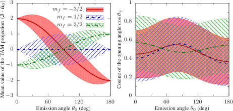
Figure 1: The mean value of the operator of the TAM projection on the direction of photon emission $\hat{{\bf n}}_{0}=\left(\sin\theta_{0},0,\cos\theta_{0}\right)$ (left panel) and the cosine of the opening angle (right panel). The recombination of the 2 keV plane-wave electron with $\mu=1/2$ into the $2p_{3/2}(m_{f})$ state of the H-like Ar ($Z=18$) ion is considered. The shadowed areas designate the dispersions.

On the left panel of this figure it is seen that for the forward and backward emission angles the TAM projection takes the well-defined values. This fact is predicted by the relation (30). From the right panel of Fig. 1 one can conclude that for all propagation directions the emitted photons do not have the well-defined opening angle $\theta_{\gamma}$ and consequently transversal momentum. This can be explained as follows. In the external field of the nucleus the momentum does not conserve and, as a result, the distribution of the momentum occurs. In accordance with definition given in Section II.1, the RR photons can not be regarded as twisted. But, these photons can neither be regarded as the plane or the spherical wave since the cosine of the opening angle always differs from 1 and 0, respectively (see the right panel of Fig. 1). Therefore, one can say that the RR photons emitted in the forward or backward directions are, in some sense, twisted.

III.2.2 Recombination of twisted electrons

Up to now we have discussed recombination of the plane-wave electrons. Nowadays, one can also use the twisted electrons instead of the conventional ones. These electrons possessing a non-zero projection of OAM onto their propagation direction can be readily produced with present experimental techniques Verbeeck_N467_301:2010 ; Uchida_N464_737:2010 ; McMorran_S331_192:2011 ; Grillo_PRL114_034801:2015 ; Mafakheri_MM21_667:2015 . It is of interest, therefore, to investigate the possibility of the TAM transfer from the twisted electron beam to the RR photons. Previously, the recombination of the vortex electrons was studied in Refs. Matula_NJP16_053024:2014 ; Zaytsev_PRA95_012702:2017 . In both works, however, no attention has been paid to the question whether the emitted radiation is twisted or not. Below we evaluate the TAM projection of the radiative photons and thereby fill in the gap.
Let us start with the brief recall of the main properties of the free twisted electrons which we take here in the form of the Bessel waves. As the vortex photons, these electrons are characterized by the following set of quantum numbers. The energy $\varepsilon$, the helicity $\mu$, and the projections of the linear $p_{z}$ and total angular $m_{e}$ momenta onto the propagation direction which is chosen as the $z$ axis. Twisted electrons possess a well-defined transversal momentum $\varkappa_{e}=\sqrt{\varepsilon^{2}-1-p_{z}^{2}}$ and the so-called opening angle $\theta_{e}=\arctan\left(\varkappa_{e}/p_{z}\right)$. The wave function of the state with the quantum numbers listed above have an inhomogeneous probability distribution and an inhomogeneous probability current density (see, e.g., Ref. Zaytsev_PRA95_012702:2017 ). Due to this feature, the relative position of the target with respect to the scattering electron and the type of the target become important. Here we consider two types of targets, viz. a single ion and an infinitely extended (macroscopic) target.

Single ion

Having discussed the basic properties of the twisted electrons, we are ready to study their interaction with ionic targets. First, we will consider the case of electron recombination with a single bare nucleus placed at some well-defined position inside the vortex electron beam. The density matrix for such a scenario can be written as

$$\left\langle{\bf k}\lambda\left|\rho^{(\rm tw,sngl)}_{\varkappa_{e}m_{e}p_{z}\mu;fm_{f}}({\bf b})\right|{\bf k}^{\prime}\lambda^{\prime}\right\rangle=\tau^{(\rm tw)}_{\varkappa_{e}m_{e}p_{z}\mu;fm_{f},{\bf k}\lambda}({\bf b})\tau^{(\rm tw)*}_{\varkappa_{e}m_{e}p_{z}\mu;fm_{f},{\bf k}^{\prime}\lambda^{\prime}}({\bf b}).$$ (31)

The amplitude of this process can be constructed from the plane-wave electron RR amplitude as follows Zaytsev_PRA95_012702:2017

$$\tau^{(\rm tw)}_{\varkappa_{e}m_{e}p_{z}\mu;fm_{f},{\bf k}\lambda}({\bf b})=i^{\mu-m_{e}}\int\frac{e^{im_{e}\varphi_{p}}}{2\pi p_{\perp}}\delta(p_{\parallel}-p_{z})\delta(p_{\perp}-\varkappa_{e})e^{i{\bf p}\cdot{\bf b}}\tau^{(\rm pl)}_{{\bf p}\mu;fm_{f},{\bf k}\lambda}d{\bf p},$$ (32)

where ${\bf b}=\left(b\cos\varphi_{b},b\sin\varphi_{b},0\right)$ is the impact parameter, i.e. the distance from the target ion to the central ($z$) axis of the incident vortex electron beam. Substituting the density matrix (31) into Eq. (3) one can evaluate the mean value of the TAM operator projection onto the direction of the photon emission $\hat{{\bf n}}_{0}$ and thereby find out whether the emitted photons are twisted or not.
The most interesting situation occurs when the ion is placed in the center of the vortex electron beam (${\bf b}=0$). In this case, it can be analytically shown that for the forward photon emission, $\hat{{\bf n}}_{0}=\hat{\bf e}_{z}$,

$$\left\langle J_{z}\right\rangle^{(b=0)}_{\rm tw}=m_{e}-m_{f},\quad\Delta^{\rm(b=0)}_{J}=0.$$ (33)

This means that the radiative photons propagating along the $z$ axis do carry the well-defined projection of the TAM onto their propagation direction. And this projection is determined solely by the TAM projections of the initial $m_{e}$ and final $m_{f}$ electrons states. This is explained as follows. For ${\bf b}=0$ the entire system possesses the azimuthal symmetry with respect to the $z$ axis. As a result, the angular momentum projection on this axis is conserved and the TAM projection of the twisted electron $m_{e}$ is equal to the sum of $m_{f}$ and TAM projection of the emitted photon. This is expressed by Eq. (33)
The angular momentum properties of the RR photons emitted into some arbitrary direction $\hat{{\bf n}}_{0}\neq\hat{\bf e}_{z}$ are presented in Fig. 2.

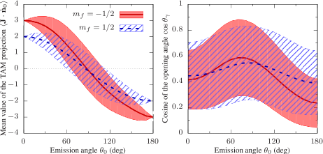
Figure 2: The mean value of the operator of the TAM projection on the direction of photon emission $\hat{{\bf n}}_{0}=\left(\sin\theta_{0},0,\cos\theta_{0}\right)$ (left panel) and the cosine of the opening angle (right panel). The recombination of the 2 keV twisted electron with $m_{e}=5/2$, $\mu=1/2$, and $\theta_{p}=30^{\circ}$ into the ground $1s(m_{f})$ state of the H-like Ar ($Z=18$) ion is considered. It is assumed that the ion is placed on the $z$ axis (${\bf b}=0$). The shadowed areas designate the dispersions of the average values.

From the left panel of this figure one can see that the photons emitted in the directions $\hat{{\bf n}}_{0}\neq\pm\hat{\bf e}_{z}$ do not possess a well-defined value of the TAM projection onto the propagation direction. From the right panel of Fig. 2 it is seen that the emitted photons do not have a well-defined opening angle $\theta_{\gamma}$. However, as in the case of the plane-wave electron recombination, we can say that the RR photons emitted in the forward or backward directions are, in some sense, twisted.
Up to now we discussed the case when the ion was placed on the electron vortex line, ${\bf b}=0$. If the ion is displaced from this axis by the impact parameter ${\bf b}$, the rotational symmetry is broken. In this case, the projection of the TAM of the RR photon is not well-defined. It is clearly seen from Fig. 3, where the results for the twisted electron RR with the bare argon nucleus being shifted from the $z$ axis are depicted.

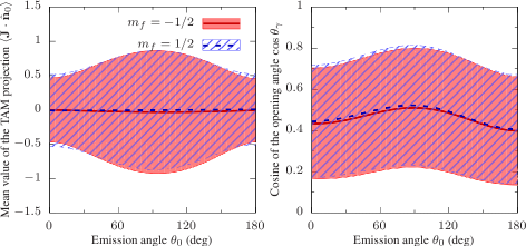
Figure 3: The mean value of the operator of the TAM projection on the direction of photon emission $\hat{{\bf n}}_{0}=\left(\sin\theta_{0},0,\cos\theta_{0}\right)$ (left panel) and the cosine of the opening angle (right panel). The recombination of the 2 keV twisted electron with $m=5/2$, $\mu=1/2$, and $\theta_{p}=30^{\circ}$ into the ground $1s(m_{f})$ state of the H-like Ar ($Z=18$) ion is considered. It is assumed that the ion is shifted along the $x$ axis from the electron propagation direction on 1 nm. The shadowed areas designate the dispersions of the average values.

It is also worth mentioning that the dependence on the TAM projection of the incident twisted electron $m_{e}$ is almost absent.

Macroscopic target

The single-ion target is interesting from theoretical viewpoint but it can not be realized in experiment. We consider, therefore, a more realistic scenario in which the twisted electron beam collides with a macroscopic target, which we describe as an incoherent superposition of ions being homogeneously distributed. The density matrix for this case is given by Zaytsev_PRA95_012702:2017

$$\left\langle{\bf k}\lambda\left|\rho^{(\rm tw,mac)}_{\varkappa_{e}m_{e}p_{z}\mu;fm_{f}}\right|{\bf k}^{\prime}\lambda^{\prime}\right\rangle=\int\frac{d{\bf b}}{\pi R^{2}}\left\langle{\bf k}\lambda\left|\rho^{(\rm tw,sngl)}_{\varkappa_{e}m_{e}p_{z}\mu;fm_{f}}({\bf b})\right|{\bf k}^{\prime}\lambda^{\prime}\right\rangle,$$ (34)

where $1/(\pi R^{2})$ is the cross section area with $R$ being the radius of the cylindrical box. In the case of the twisted electron RR with the macroscopic target the emitted photon, unfortunately, does have neither a well-defined TAM projection nor a well-defined opening angle.

IV CONCLUSION

In the present work, we described the simple theoretical method for the evaluation of the “twistedness” of the photons emitted in basic atomic processes. As the applications of the proposed method, we evaluated the TAM projection and its dispersion for the plane-wave, spherical-wave, and twisted photons. We have also analyzed the “twistedness” of the photons emitted in the radiative recombination of electrons with the bare argon nuclei. Two different situations have been considered. In the first scenario it was assumed that the incident electron was prepared in the plane-wave state, while the twisted state was considered in the second one. It was found that in the first scenario the RR photons emitted in the forward or backward directions have the well-defined TAM projection onto this direction. For these photons the TAM projection is determined solely by the polarizations of the incident plane-wave electron and by the magnetic quantum number of the residual ion. In the second scenario, the most interesting result has been obtained for the RR with the ion placed in the center of the electron beam. In this case the recombination radiation propagating in the forward direction does possess a well-defined TAM projection onto this direction. This result does not retain for the target ion being shifted from the propagation direction as well as for the recombination with the macroscopic target. And, although, for the both scenarios the emitted photons do not have well-defined opening angles, we believe that the RR photons for the forward or backward emission directions are, in some sense, twisted.
To summarize, the developed method allows one to find out whether the emitted photons are twisted without going into details of the process. This method can be readily extended to the evaluation of the “twistedness” of other particles.

References

- (1) G. Molina-Terriza, J. P. Torres, and L. Torner, Nat. Phys. 3, 305 (2007).
- (2) A. M. Yao and M. J. Padgett, Adv. Opt. Photon. 3, 161 (2011).
- (3) J. P. Torres and L. Torner, Twisted Photons: Applications of Light with Orbital Angular Momentum (Wiley-VCH, Weinheim, 2011).
- (4) The Angular Momentum of Light, edited by D. L. Andrews and M. Babiker (Cambridge University, Cambridge, England, 2013).
- (5) N. Bozinovic, Y. Yue, Y. Ren, M. Tur, P. Kristensen, H. Huang, A. E. Willner, and S. Ramachandran, Science 340, 1545 (2013).
- (6) G. Gibson, J. Courtial, M. Padgett, M. Vasnetsov, V. Pas’ko, S. Barnett, and S. Franke-Arnold, Opt. Express 12, 5448 (2004).
- (7) J. Wang, J.-y. Yang, I. M. Fazal, N. Ahmed, Y. Yan, H. Huang, Y. Ren, Y. Yue, S. Dolinar, M. Tur, and A. E. Willner, Nat. Photonics 6, 488 (2012).
- (8) T. Su, R. P. Scott, S. S. Djordjevic, N. K. Fontaine, D. J. Geisler, X. Cai, and S. J. B. Yoo, Opt. Express 20, 9396 (2012).
- (9) V. D’Ambrosio, N. Spagnolo, L. Del Re, S. Slussarenko, Y. Li, L. C. Kwek, L. Marrucci, S. P. Walborn, L. Aolita, and F. Sciarrino, Nat. Commun. 4, 2432 (2013).
- (10) D. G. Grier, Nature (London) 424, 810 (2003).
- (11) C. T. Schmiegelow and F. Schmidt-Kaler, Eur. Phys. J. D 66, 157 (2012).
- (12) A. Afanasev, C. E. Carlson, and A. Mukherjee, Phys. Rev. A 88, 033841 (2013).
- (13) H. M. Scholz-Marggraf, S. Fritzsche, V. G. Serbo, A. Afanasev, and A. Surzhykov, Phys. Rev. A 90, 013425 (2014).
- (14) A. Surzhykov, D. Seipt, V. G. Serbo, and S. Fritzsche, Phys. Rev. A 91, 013403 (2015).
- (15) C. T. Schmiegelow, J. Schulz, H. Kaufmann, T. Ruster, U. G. Poschinger, and F. Schmidt-Kaler, Nat. Commun. 7, 12998 (2016).
- (16) R. A. Müller, D. Seipt, R. Beerwerth, M. Ornigotti, A. Szameit, S. Fritzsche, and A. Surzhykov, Phys. Rev. A 94, 041402(R)(2016).
- (17) D. Seipt, R. A. Müller, A. Surzhykov, and S. Fritzsche, Phys. Rev. A 94, 053420 (2016).
- (18) A. Surzhykov, D. Seipt, and S. Fritzsche, Phys. Rev. A 94, 033420 (2016).
- (19) T. Kaneyasu, Y. Hikosaka, M. Fujimoto, T. Konomi, M. Katoh, H. Iwayama, and E. Shigemasa, Phys. Rev. A 95, 023413 (2017).
- (20) S. Stock, A. Surzhykov, S. Fritzsche, and D. Seipt, Phys. Rev. A 92, 013401 (2015).
- (21) L. Zhang, B. Shen, X. Zhang, S. Huang, Y. Shi, C. Liu, W. Wang, J. Xu, Z. Pei, and Z. Xu, Phys. Rev. Lett. 117, 113904 (2016).
- (22) U. D. Jentschura and V. G. Serbo, Phys. Rev. Lett. 106, 013001 (2011); Eur. Phys. J. C 71, 1571 (2011).
- (23) I. P. Ivanov, Phys. Rev. D 83, 093001 (2011).
- (24) I. P. Ivanov and V. G. Serbo, Phys. Rev. A 84, 033804 (2011).
- (25) C. Hernaández-García, A. Picón, J. S. Román, and L. Plaja, Phys. Rev. Lett. 111, 083602 (2013).
- (26) L. Rego, J. S. Román, A. Picón, L. Plaja, and C. Hernández-García, Phys. Rev. Lett. 117, 163202 (2016).
- (27) F. Kong, C. Zhang, F. Bouchard, Z. Li, G. G. Brown, D. H. Ko, T. J. Hammond, L. Arissian, R. W. Boyd, E. Karimi, and P. B. Corkum, Nat. Commun. 8, 14970 (2017).
- (28) D. Gauthier, P. R. Ribic, G. Adhikary, A. Camper, C. Chappuis, R. Cucini, L. F. DiMauro, G. Dovillaire, F. Frassetto, R. Géneaux, P. Miotti, L. Poletto, B. Ressel, C. Spezzani, M. Stupar, and T. Ruchon, Nat. Commun. 8, 14971 (2017).
- (29) O. Matula, A. G. Hayrapetyan, V. G. Serbo, A. Surzhykov, and S. Fritzsche, J. Phys. B 46, 205002 (2013).
- (30) V. V. Balashov, A. N. Grum-Grzhimailo, and N. M. Kabachnik, Polarization and Correlation Phenomena in Atomic Collisions (Springer, Boston, 2000).
- (31) A. I. Akhiezer and V. B. Berestetskii, Quantum Electrodynamics (Interscience, New York, 1965).
- (32) M. E. Rose, Elementary Theory of Angular Momentum (Wiley, New York, 1957).
- (33) D. A. Varshalovich, A. N. Moskalev, and V. K. Khersonskii, Quantum Theory of Angular Momentum (World Scientific, Singapore, 1988).
- (34) V. B. Berestetsky, E. M. Lifshitz, and L. P. Pitaevskii, Quantum Electrodynamics (Butterworth-Heinemann, Oxford, 2006).
- (35) J. Eichler and Th. Stöhlker, Phys. Rep. 439, 1 (2007).
- (36) J. Eichler and W. Meyerhof, Relativistic Atomic Collisions (Academic, San Diego, 1995).
- (37) M. E. Rose, Relativistic Electron Theory (Wiley, New York, 1961).
- (38) R. H. Pratt, A. Ron, and H. K. Tseng, Rev. Mod. Phys. 45, 273 (1973); 45, 663(E) (1973).
- (39) J. Verbeeck, H. Tian, and P. Schattschneider, Nature 467, 301 (2010).
- (40) M. Uchida and A. Tonomura, Nature 464, 737 (2010).
- (41) B. J. McMorran, A. Agrawal, I. M. Anderson, A. A. Herzing, H. J. Lezec, J. J. McClelland, and J. Unguris, Science 331, 192 (2011).
- (42) V. Grillo, G. C. Gazzadi, E. Mafakheri, S. Frabboni, E. Karimi, and R. W. Boyd, Phys. Rev. Lett. 114, 034801 (2015).
- (43) E. Mafakheri, V. Grillo, R. Balboni, G. C. Gazzadi, C. Menozzi, S. Frabboni, E. Karimi, and R. W. Boyd, Microsc. Microanal. 21, 667 (2015).
- (44) O. Matula, A. G. Hayrapetyan, V. G. Serbo, A. Surzhykov, and S. Fritzsche, New J. Phys. 16, 053024 (2014).
- (45) V. A. Zaytsev, V. G. Serbo, and V. M. Shabaev, Phys. Rev. A 95, 012702 (2017).