Contingent Derivatives and regularization for noncoercive inverse problems

Abstract

We study the inverse problem of parameter identification in non-coercive variational problems that commonly appear in applied models. We examine the differentiability of the set-valued parameter-to-solution map by using the first-order and the second-order contingent derivatives. We explore the inverse problem by using the output least-squares and the modified output least-squares objectives. By regularizing the non-coercive variational problem, we obtain a single-valued regularized parameter-to-solution map and investigate its smoothness and boundedness. We also consider optimization problems using the output least-squares and the modified output least-squares objectives for the regularized variational problem. We give a complete convergence analysis showing that for the output least-squares and the modified output least-squares, the regularized minimization problems approximate the original optimization problems suitably. We also provide the first-order and the second-order adjoint method for the computation of the first-order and the second-order derivatives of the output least-squares objective. We provide discrete formulas for the gradient and the Hessian calculation and present numerical results.

2000 Mathematics Subject Classification 35R30, 49N45, 65J20, 65J22, 65M30

1 Introduction

Non-coercive variational problems frequently emerge from applied models (see [21]). However, often less general versions of such models are studied under the coercivity assumption so that useful technical tools can be employed. For instance, in all the available literature on the inverse problem of identifying a variable parameter in elliptic partial differential equations using a variational framework, the bilinear form has always been chosen to be coercive. The coercivity ensures that the variational problem is uniquely solvable and retains stability on the data perturbation. Under coercivity, the parameter-to-solution map is single-valued, well-defined, and infinitely differentiable. Furthermore, coercivity also plays a decisive role in local stability estimates, see [27]. Although the solvability of a noncoercive variational problem can be ensured by other tools (see [3]), the parameter-to-solution map, in this case, is a set-valued map. Therefore, for parameter identification in noncoercive variational problems, to derive optimality conditions, one has to employ a suitable notion of a derivative of set-valued maps. Therefore, the known techniques need to be altered significantly to cope with the involvement of such technical tools. For an overview of the recent developments in the vibrant and expanding field of inverse problems, the reader is referred to [2, 5, 6, 10, 11, 13, 14, 17, 22, 23, 33, 30, 34, 36, 37, 38, 40].

A prototypical example of a non-coercive variational problem is the weak formulation of pure Neumann boundary value problem (BVP): Given a bounded open domain $\Omega$ and the unit outer unit normal $n$, consider the problem of finding $u$ such that

(1) $$-\nabla\cdot(a\nabla u)=f\ \ \mbox{in}\ \Omega,\ \frac{\partial u}{\partial n}=g\ \ \mbox{on}\ \partial\Omega,$$

where $\frac{\partial u}{\partial n}$ is the outer normal derivative of $u$ on the boundary $\partial\Omega$, and $f$ and $g$ are two given functions. It is known that the weak form of the above BVP leads to a noncoercive bilinear form. Moreover, (1) is solvable only under the compatibility condition

$$\int_{\Omega}f+\int_{\partial\Omega}g=0,$$

whereas, as a consequence of Fredholm alternate, there are infinitely many solutions, with any two solutions only differing by a constant. Furthermore, among these solutions, there is a unique solution under the additional constraint $\int_{\Omega}u=0$.

All the research on the inverse problems of parameter identification in pure Neumann BVP, the constraint $\int_{\Omega}u=0$ and the compatibility condition have been imposed so that the parameter-to-solution map $a\to u(a)$ is well-defined and single-valued.

The primary objective of this work is to conduct a thorough study of the inverse problem of parameter identification in noncoercive variational problems. However, before going into the details of the main contribution of this article, we provide a brief review of the existing approaches for parameter identification in partial differential equations (PDEs) and variational problems by focusing on the role of coercivity. Let $B$ be a Banach space and let $A$ be a closed, and convex subset of $B$ with a nonempty interior. Given a Hilbert space $V$, let $T:B\times V\times V\rightarrow\mathbb{R}$ be a trilinear form with $T(a,u,v)$ symmetric in $u$, $v$, and let $m$ be a bounded linear functional on $V$. Assume there are constants $\alpha>0$ and $\beta>0$ such that the following continuity (cf. (2)) and coercivity (cf. (3)) conditions hold:

(2) $$T(a,u,v) \leq\beta\|a\|_{B}\|u\|_{V}\|v\|_{V},\ \ \text{for all}\ u,v\in V,\ a\in B,$$

(3) $$T(a,u,u) \geq\alpha\|u\|_{V}^{2},\ \text{for all}\ u\in V,\ a\in A.$$

Consider the following variational problem: Given $a\in A$, find $u=u(a)\in V$ such that

(4) $$T(a,u,v)=m(v),\ \ \text{for every}\ v\in V.$$

Due to the conditions imposed on the trilinear map $T$, the Riesz representation theorem ensures that for any $a\in A$, variational problem (4) admits a unique solution $u(a)$ (see [21]). The inverse problem now seeks the parameter $a$ in (4) from a measurement $z$ of $u$. This inverse problem is often studied in an optimization framework, either formulating the problem as an unconstrained optimization problem or treating it as a constrained optimization problem in which the variational problem itself is the constraint.

Given a Banach space $Z\supseteq V$ equipped with the norm $\|\cdot\|_{Z}$, the most commonly adopted optimization framework minimizes the following output least-squares (OLS) functional

(5) $$J_{1}(a):=\|u(a)-z\|^{2}_{Z}$$

where $z\in Z$ is the data (the measurement of $u$) and $u(a)$ solves the variational form (4).

For an insight into the abstract framework, consider the boundary value problem (BVP)

(6) $$-\nabla\cdot(a\nabla u)=f\ \ \mbox{in}\ \Omega,\ u=0\ \ \mbox{on}\ \partial\Omega,$$

where $\Omega$ is a suitable domain in $\mathbb{R}^{2}$ or $\mathbb{R}^{3}$ and $\partial\Omega$ is its boundary. BVP (6) models useful real-world problems and has been studied in detail. For example, in (6), $u=u(x)$ may represent the steady-state temperature at a point $x$ of a body; then $a$ would be a variable thermal conductivity coefficient, and $f$ the external heat source. BVP (6) also models underground steady state aquifers in which the parameter $a$ is the aquifer transmissivity coefficient, $u$ is the hydraulic head, and $f$ is the recharge. The inverse problem in the context of (6) is to estimate the parameter $a$ from a measurement $z$ of the solution $u$.

For (6) with $Z=L_{2}(\Omega)$, optimization problem (5) reduces to minimizing

(7) $$\tilde{J}_{1}(a):=\int_{\Omega}(u(a)-z)^{2},$$

where $z$ is the measurement of $u$ and $u(a)$ solves the variational form of (6) given by

(8) $$\int_{\Omega}a\nabla u\cdot\nabla v=\int_{\Omega}fv,\ \ \text{for all}\,v\in H_{0}^{1}(\Omega).$$

A variant of (5) is the following modified OLS functional (MOLS) introduced in [19]

(9) $$J_{2}(a)=T(a,u(a)-z,u(a)-z),$$

where $z$ is the data and $u(a)$ solves (4). In [19], the author established that (9) is convex and used it to estimate the Lamé moduli in the equations of isotropic elasticity. Studies related to MOLS functional and its extensions can be found in [15, 20, 26].

The MOLS functional, given in (9), was inspired by Knowles [35] who minimized a coefficient-dependent norm

(10) $$\tilde{J}_{2}(a):=\int_{\Omega}a\nabla(u(a)-z)\cdot\nabla(u(a)-z),$$

where $z$ is the measurement of $u$, and $u(a)$ solves (8).

Besides the OLS functional and the MOLS functional, there are other approaches. The equation error method (cf. [1, 28, 29]), for (6), consists of minimizing the functional

$$\tilde{J}_{3}(a):=\|\nabla(a\nabla z)+f\|^{2}_{H^{-1}(\Omega)}$$

where $H^{-1}(\Omega)$ is the dual of $H_{0}^{1}(\Omega)$ and $z$ is the data. In [16], the equation error approach was explored in an abstract framework.

Finally, we recall the following two results from [19] for the parameter-to-solution map.

Lemma 1.1.

For any $a\in A$, the solution $u(a)$ of the variational problem (4) satisfies $\|u(a)\|_{V}\leq\alpha^{-1}\|m\|_{V^{*}}$. Moreover, for any $a,b\in A$, we have

(11) $$\|u(a)-u(b)\|_{V}\leq\min\left\{\frac{\beta}{\alpha}\|u(a)\|_{V},\frac{\beta}{\alpha}\|u(b)\|_{V},\frac{\beta}{\alpha^{2}}\|m\|_{V^{*}}\right\}\|b-a\|_{B}.$$

Lemma 1.2.

For each $a$ in the interior of $A$, the solution $u(a)$ of the variational problem (4) is infinitely differentiable at $a$. Given $u=u(a)$, the first derivative $Du(a)\delta a$ of $u(a)$ in the direction $\delta a$, is the unique solution of the following variational equation

(12) $$T(a,Du(a)\delta a,v)=-T(\delta a,u,v),\ \forall\,v\in V.$$

Furthermore, the second derivative $D^{2}u(a)(\delta a_{1},\delta a_{2})$ of $u(a)$ in the direction $(\delta a_{1},\delta a_{2})$, is the unique solution of the following variational equation

(13) $$T(a,D^{2}u(a)(\delta a_{1},\delta a_{2}),v)=-T(\delta a_{2},Du(a)\delta a_{1},v)-T(\delta a_{1},Du(a)\delta a_{2},v),\ \forall\,v\in V.$$

Moreover, the following bounds hold:

(14) $$\|Du(a)\| \leq \frac{\beta}{\alpha}\|u(a)\|_{V} \leq\frac{\beta}{\alpha^{2}}\|m\|_{V^{*}},$$

(15) $$\left\|D^{2}u(a)\right\| \leq \,\frac{2\beta^{2}}{\alpha^{2}}\|u(a)\|_{V} \leq\frac{2\beta^{2}}{\alpha^{3}}\|m\|_{V^{*}}.$$

In all of the above results, coercivity condition (3) played the most crucial role. It gives the unique solvability of variational problem (4), proves bound on the parameter-to-solution map, establishes its Lipschitz continuity and infinite differentiability. As another useful consequences of the coercivity, the first-order and the second-order derivatives of the parameter-to-solution maps are the unique solutions of the variational problems (12) and (13). Moreover, the useful bounds (14) and (15) also hold due to the coercivity.

This work aims to study the inverse problem of parameter identification in noncoercive variational problems with perturbed data. Our main contributions are as follows:

1. Assuming that the noncoercive variational problem is solvable, we give a derivative characterization for the set-valued parameter-to-solution map by using the first-order and the second-order contingent derivatives. To our knowledge, this is the first use of such tools from variational analysis in the study of inverse problems.

2. We study the inverse problem by posing optimization problems using the output least-squares and the modified output least-squares functionals for the set-valued parameter to solution map. We regularize the noncoercive variational problem and obtain the single-valued regularized parameter-to-selection map and explore its smoothness. We consider optimization problems using the output least-squares and the modified output least-squares for the regularized variational problem. We prove that the MOLS objective is convex and give a complete convergence analysis showing that the regularized problems approximate the original problem suitably.

3. To compute the first-order and the second-order derivative of the OLS functional, we give first-order, and second-order adjoint methods in the continuous setting. We provide a discretization scheme and give discrete formulas for the OLS and the MOLS functionals and their gradient and Hessian calculation. As a byproduct of our study, we obtain new insight into the case when the actual trilinear form is coercive, however, for the computations, only its contaminated analog is available which is noncoercive. All the conditions imposed for the convergence analysis are satisfied in this case of practical importance.

We organize the contents of this paper into seven sections. Section 2 introduces the inverse problem and explores the smoothness of the set-valued parameter-to-solution map. Section 3 investigates the inverse problem by using the output-least squares approach and the modified output least squares approach. Section 4 is devoted to the first-order and the second-order adjoint approaches. Section 5 provides a detailed computational framework including the discrete gradient and Hessian formulae. In Section 6, we report the outcome of some preliminary numerical experiments. The paper concludes with some remarks.

2 Set-valued Solution Map for a Noncoercive Variational Problem

For convenience, we recall the general setting once again. Let $B$ be a Banach space, let $A\subset B$ be a nonempty, closed, and convex set. Let $V$ be a Hilbert space continuously imbedded in a Hilbert space $Z$. Let $T:B\times V\times V\rightarrow\mathbb{R}$ be a trilinear form with $T(a,u,v)$ symmetric in $u$, $v$. Let $m$ be a bounded linear functional on $V$. Assume that $T$ satisfies the continuity assumption (2) and the following positivity condition:

(16) $$T(a,u,u)\geq 0,\ \text{for all}\ u\in V,\ a\in A.$$

Consider the noncoercive variational problem: Given $a\in A$, find $u=u(a)\in V$ such that

(17) $$T(a,u,v)=m(v),\ \ \text{for every}\ v\in V.$$

Since we do not impose the coercivity condition (see (3)) on $T$, additional conditions are necessary to ensure that (17) is solvable. For example, recession analysis can be used to ensure that (17) is solvable but such conditions don’t guarantee that the solution is unique (see [21]). Therefore, it is natural to study the behavior of the set-valued parameter-to-solution map. For a given parameter $a\in A$, by $\mathcal{U}(a)$ we denote the set of all solutions of variational equation (17). In the following, we assume that for each $a\in A$, the set $\mathcal{U}(a)$ is nonempty. The following lemma provides additional information:

Lemma 2.1.

For any $a\in A$, the set of all solutions $\mathcal{U}(a)$ of (17) is closed and convex.

Proof 2.2.

The proof follows at once from the definition of the set-valued parameter-to-solution map $\mathcal{U}:A\rightrightarrows V$. Indeed, let $u$ and $w$ be two arbitrary elements in $\mathcal{U}(a)$. Then, for every $v\in V$, we have $T(a,u,v)=m(v)$ and $T(a,w,v)=m(v)$. We take $t\in[0,1]$ and note that for every $v\in V$, we have $T(a,tu,v)=tm(v)$ and $T(a,(1-t)u,v)=(1-t)m(v)$. We combine these equations to note that for every $v\in V$, we have $T(a,tu+(1-t)w,v)=m(v)$. Consequently, $tu+(1-t)w\in\mathcal{U}(a)$ confirming the convexity of $\mathcal{U}(a)$. The set $\mathcal{U}(a)$ is closed due to the continuity of the trilinear form $T$. The proof is complete.

Our goal is to obtain a derivative characterization for the set-valued parameter-to-solution map. In the literature, a variety of derivative concepts have been employed to differentiate set-valued maps (see [32]). We will use first-order and second-order contingent derivatives of the parameter-to-solution set-valued map $\mathcal{U}:A\rightrightarrows V$. These derivatives are defined by using the contingent cone and the second-order contingent set which we recall now.

Definition 2.3.

Let $X$ be a normed space, let $S\subset X$ and let $\bar{z}\in\operatorname{\mathrm{cl}}(S)$ (closure of $S$).

1. The contingent cone $C(S,\bar{z})$ of $S$ at $\bar{z}$ is the set of all $z\in X$ such that there are sequences $\{t_{n}\}\subset\mathbb{P}:=\{t\in\mathbb{R}\,|\ t>0\}$ and $\{z_{n}\}\subset X$ with $t_{n}\downarrow 0$ and $z_{n}\to z$ such that $\bar{z}+t_{n}z_{n}\in S$, for every $n\in\mathbb{N}$.

2. The second-order contingent set $C^{2}(S,\bar{z},w)$ of $S$ at $\bar{z}\in\operatorname{\mathrm{cl}}(S)$ in the direction $w\in X$ is the set of all $z\in S$ such that there are a sequence $\{z_{n}\}\subset X$ with $z_{n}\to z$ and a sequence $\{t_{n}\}\subset\mathbb{P}$ with $t_{n}\downarrow 0$ such that $\bar{z}+t_{n}w+t_{n}^{2}z_{n}/2\in S$, for every $n\in\mathbb{N}$.

Remark 2.4.

It is known that the contingent cone $C(S,\bar{z})$ is a nonempty closed cone. However, $C^{2}(S,\bar{z},w)$ is only a closed set (possibly empty), non-connected in general, and it may be nonempty only if $w\in C(S,\bar{z})$. Details of these concepts can be found in [7, 8, 32].

Next we collect some notions for set-valued maps. Given normed spaces $X$ and $Y$, let $F:X\rightrightarrows Y$ be a set-valued map. The (effective) domain and the graph of $F$ are defined by $\text{dom}(F):=\{x\in X|\quad F(x)\not=\emptyset\}$, and $\text{graph}(F):=\{(x,y)\in X\times Y|\quad y\in F(x)\}$.

We now introduce first-order and second-order derivatives of set-valued maps.

Definition 2.5.

Let $X$ and $Y$ be normed spaces, let $F:X\rightrightarrows Y$ be a set-valued map, and let $(\bar{x},\bar{y})\in\operatorname{\mathrm{graph}}(F)$. Then the contingent derivative of $F$ at $(\bar{x},\bar{y})$ is the set-valued map $DF(\bar{x},\bar{y}):X\rightrightarrows Y$ given by

$$DF(\bar{x},\bar{y})(x):=\{y\in Y\,|\ (x,y)\in C(\operatorname{\mathrm{graph}}(F),(\bar{x},\bar{y}))\}.$$

Moreover, the second-order contingent derivative of $F$ at $(\bar{x},\bar{y})$ in the direction $(\bar{u},\bar{v})$ is the set-valued map $D^{2}F(\bar{x},\bar{y},\bar{u},\bar{v}):X\rightrightarrows Y$ defined by

$$D^{2}F(\bar{x},\bar{y},\bar{u},\bar{v})(x):=\left\{y\in Y\,|\ (x,y)\in C^{2}(\operatorname{\mathrm{graph}}(F),(\bar{x},\bar{y}),(\bar{u},\bar{v}))\right\}.$$

The above derivatives have been used extensively in nonsmooth and variational analysis, viability theory, set-valued optimization and numerous other related disciplines, see [32].

We have the following derivative characterization for the parameter-to-solution map:

Theorem 2.6.

For $\bar{a}\in A$, let $\bar{u}\in\mathcal{U}(\bar{a})$ be a given point. Assume that the first-order contingent derivative $D\mathcal{U}(\bar{a},\bar{u}):B\rightrightarrows V$ of the set-valued parameter-to-solution map $\mathcal{U}:A\rightrightarrows V$ at the point $(\bar{a},\bar{u})\in\text{graph}(\mathcal{U})$ exists. Then for any given direction $\delta a\in B$, any element $\delta u\in D\mathcal{U}(\bar{a},\bar{u})(\delta a)$ satisfies the following variational problem:

(18) $$T(\bar{a},\delta u,v)=-T(\delta a,\bar{u},v),\quad\text{for every}\ v\in V.$$

Proof 2.7.

For the given element $(\bar{a},\bar{u})\in\text{graph}(\mathcal{U})$ and the given direction $\delta a$, for any $\delta u\in D\mathcal{U}(\bar{a},\bar{u})(\delta a)$, we have

$$(\delta a,\delta u)\in\text{graph}(D\mathcal{U}(\bar{a},\bar{u}))=C(\text{graph}(\mathcal{U}),(\bar{a},\bar{u})),$$

and by the definition of the contingent cone, there are sequences $\{t_{n}\}\subset\mathbb{P}$ and $\{(a_{n},u_{n})\}$ with $t_{n}\to 0$ and $(a_{n},u_{n})\to(\delta a,\delta u)$ such that $(\bar{a}+t_{n}a_{n},\bar{u}+t_{n}u_{n})\in\text{graph}(\mathcal{U})$, or equivalently $\bar{u}+t_{n}u_{n}\in\mathcal{U}(\bar{a}+t_{n}a_{n})$, which, by the definition of the map $\mathcal{U}:A\rightrightarrows V$, implies that

$$T(\bar{a}+t_{n}a_{n},\bar{u}+t_{n}u_{n},v)=m(v),\quad\text{for every}\ v\in V,$$

and after a rearrangement of this variational problem, we obtain

$$T(\bar{a},\bar{u},v)+t_{n}T(\bar{a},u_{n},v)+t_{n}T(a_{n},\bar{u},v)+t_{n}^{2}T(a_{n},u_{n},v)=m(v),\quad\text{for every}\ v\in V.$$

The condition $(\bar{a},\bar{u})\in\text{graph}(\mathcal{U})$ implies that $T(\bar{a},\bar{u},v)=m(v)$, for every $v\in V$, and hence

$$T(\bar{a},u_{n},v)=-T(a_{n},\bar{u},v)-t_{n}T(a_{n},u_{n},v),\quad\text{for every}\ v\in V.$$

By passing the above equation to the limit $n\to\infty$, we obtain

$$T(\bar{a},\delta u,v)=-T(\delta a,\bar{u},v),\quad\text{for every}\ v\in V,$$

and the desired identity (18) is proved. The proof is complete.

Remark 2.8.

If the trilinear form $T$ satisfies coercivity condition (3), then for every parameter $\bar{a}\in A$, variational problem (17) has a unique solution $\bar{u}=u(\bar{a})$, that is, the map $\bar{a}\to u(\bar{a})$ is well-defined and single-valued. Moreover, for any $a$ in the interior of $A$ and any direction $\delta a$, the Fréchet derivative $\delta u=D\bar{u}(\bar{a})(\delta a)$ is the unique solution of the variational problem (12) which is entirely comparable to the characterization (18).

The following is the characterization of the second-order contingent derivative:

Theorem 2.9.

For any $\bar{a}\in A$, let $\bar{u}\in\mathcal{U}(\bar{a})$ be a given element. Assume that second-order contingent derivative of the parameter-to-solution set-valued map $\mathcal{U}:A\rightrightarrows V$ at $(\bar{a},\bar{u})$ in the direction $(\delta a,\delta u)\in\text{graph}(D\mathcal{U}(\bar{a},\bar{u}))$ exists. Then for any given direction $\delta\tilde{a}\in B$, any element $\delta^{2}u\in D^{2}\mathcal{U}(\bar{a},\bar{u},\delta a,\delta u)(\delta\tilde{a})$ satisfies the variational problem:

(19) $$T(\bar{a},\delta^{2}u,v)=-2T(\delta a,\delta u,v)-T(\delta\tilde{a},\bar{u},v),\quad\text{for every}\ v\in V.$$

Proof 2.10.

For the given $(\bar{a},\bar{u})\in\text{graph}(\mathcal{U})$ and the given $(\delta a,\delta u)\in\text{graph}(D\mathcal{U}(\bar{a},\bar{u}))$, let $\delta^{2}u\in D^{2}\mathcal{U}(\bar{a},\bar{u},\delta a,\delta u)(\delta\tilde{a})$. Then, we have

$$(\delta\tilde{a},\delta^{2}u)\in\text{graph}(D^{2}\mathcal{U}(\bar{a},\bar{u},\delta a,\delta u))=C^{2}(\text{graph}(\mathcal{U}),\bar{a},\bar{u},\delta a,\delta u).$$

Therefore, there are sequences $\{t_{n}\}\subset\mathbb{P}$ and $\{(a_{n},u_{n})\}\in\text{graph}(\mathcal{U})$ with $t_{n}\to 0$, and $(a_{n},u_{n})\to(\delta\tilde{a},\delta^{2}u)$ so that $(\bar{a}+t_{n}\delta a+\frac{1}{2}t_{n}^{2}a_{n},\bar{u}+\frac{1}{2}t_{n}\delta u+t_{n}^{2}u_{n})\in\text{graph}(\mathcal{U})$. By the definition of the parameter-to-solution map, we have

$$T(\bar{a}+t_{n}\delta a+\frac{1}{2}t_{n}^{2}a_{n},\bar{u}+t_{n}\delta u+\frac{1}{2}t_{n}^{2}u_{n},v)=m(v),\quad\text{for every}\ v\in V.$$

We simplify the above identity as follows

(20) $$T(\bar{a},\bar{u},v)+t_{n}T(\bar{a},\delta u,v)+\frac{1}{2}t_{n}^{2}T(\bar{a},u_{n},v)+t_{n}T(\delta a,\bar{u},v)+t_{n}^{2}T(\delta a,\delta u,v)\\ +\frac{1}{2}t_{n}^{3}T(\delta a,u_{n},v)+\frac{1}{2}t_{n}^{2}T(a_{n},\bar{u},v)+\frac{1}{2}t_{n}^{3}T(a_{n},\delta u,v)+\frac{1}{4}t_{n}^{4}T(a_{n},u_{n},v)=m(v),$$

which, first by using the fact that $(\bar{a},\bar{u})\in\text{graph}(\mathcal{U})$, and then by dividing both sides of the resulting identity by $t_{n}$ confirms that

$$T(\bar{a},\delta u,v)+\frac{1}{2}t_{n}T(\bar{a},u_{n},v)+T(\delta a,\bar{u},v)+t_{n}T(\delta a,\delta u,v)\\ +\frac{1}{2}t_{n}^{2}T(\delta a,u_{n},v)+\frac{1}{2}t_{n}T(a_{n},\bar{u},v)+\frac{1}{2}t_{n}^{2}T(a_{n},\delta u,v)+\frac{1}{4}t_{n}^{3}T(a_{n},u_{n},v)=0,$$

We now first use the fact that $(\delta a,\delta u)\in\text{graph}(D\mathcal{U}(\bar{a},\bar{u}))$, and then divide both sides of the resulting identity by $t_{n}$ to obtain

$$\frac{1}{2}T(\bar{a},u_{n},v)+T(\delta a,\delta u,v)+\frac{1}{2}t_{n}T(\delta a,u_{n},v)\\ +\frac{1}{2}T(a_{n},\bar{u},v)+\frac{1}{2}t_{n}T(a_{n},\delta u,v)+\frac{1}{4}t_{n}^{2}T(a_{n},u_{n},v)=0,$$

which when passed to the limit $t_{n}\to 0$, yields

$$T(\bar{a},\delta^{2}u,v)=-2T(\delta a,\delta u,v)-T(\delta\tilde{a},\bar{u},v),$$

proving (19). The proof is complete.

Note that due to the characterization of the first-order contingent derivative of the set-valued map $\mathcal{U}:A\rightrightarrows V$, variational problem (19) is equivalent to

(21) $$T(\bar{a},\delta^{2}u,v)=-2T(\delta a,\delta u,v)+T(\bar{a},\delta\tilde{u},v),$$

where $\delta\tilde{u}\in D\mathcal{U}(\bar{a},\bar{u})(\delta\tilde{a})$ and $v\in V$ is arbitrary.

Clearly, if $T$ satisfies condition (3), then the parameter-to-solution map is single-valued and infinitely differentiable in the interior of the domain. Moreover, for any $\bar{a}$ in the interior of $A$, and suitable directions $(\delta a_{1},\delta a_{2})$, the second-order derivative $D^{2}u(\bar{a})(\delta a_{1},\delta a_{2})$ is the unique solution of (13). In particular, with $\delta a=\delta a_{1}=\delta a_{2}$, we have

(22) $$T(\bar{a},D^{2}u(\bar{a})(\delta a,\delta a),v)=-2T(\delta a,Du(a)\delta a,v),\ \ \text{for every}\ v\in V.$$

We also recall that if a single-valued map $F:X\to Y$ is twice differentiable, then with $DF(x)$ and $D^{2}F(x)$ as the first-order and the second-order derivatives, we have (see [41])

$$C^{2}(\text{graph}(F),(x,F(x),v,DF(x)v))=\{(y,DF(x)y+D^{2}F(x)(v,v)),\ y\in X\}.$$

Consequently, by taking $\delta a=\delta\tilde{a}$, we have

$$\text{graph}(D^{2}\mathcal{U}(\bar{a},\bar{u},\delta a,\delta u))=\{(\delta a,D\bar{u}(\bar{a})\delta a+D^{2}\bar{u}(\bar{a})(\delta a,\delta a)),\ \delta a\in B\}$$

and, as a result, under (3), the derivative formula yields

$$T(\bar{a},D\bar{u}(\bar{a})\delta a+D^{2}\bar{u}(\bar{a})(\delta a,\delta a),v)=-2T(\delta a,D\bar{u}(\bar{a})(\delta a),v)+T(\bar{a},D\bar{u}(\bar{a})\delta a,v),\ \text{for all}\ v\in V,$$

implying that

$$T(\bar{a},D^{2}\bar{u}(\bar{a})(\delta a,\delta a),v)=-2T(\delta a,D\bar{u}(\delta)(\delta a),v),\quad\text{for every}\ v\in V,$$

which is in compliance with the second-order formula (22).

Remark 2.11.

The results given above only offer characterizations of the first-order and the second-order contingent derivatives under the critical assumption that these derivatives exist. This is a natural step as we have not identified conditions under which the variational problem is solvable. A possible extension of these results is singling out conditions ensuring the existence of solutions and then using them to verify the contingent differentiability.

3 Recasting the Inverse Problem in an Optimization Framework

3.1 The Output Least-Squares Approach

Let $\mathcal{U}:A\rightrightarrows V$ be the set-valued parameter-to-solution map which assigns to each $a\in A$, the set of all solutions $\mathcal{U}(a)$ of the noncoercive variational problem (17). We define the set-valued output least-squares map $\widehat{J}:A\rightrightarrows\mathbb{R}$ which connects to each $a\in A$, the following set

$$\widehat{J}(a):=\left\{\|u(a)-z\|^{2}_{Z}\mid\ u(a)\in\mathcal{U}(a)\right\},$$

where $z\in Z$ is the measured data.

Using the above set-valued map (and a slight abuse of the notation), we pose the following OLS-based optimization problem

(23) $$\min_{a\in A}\widehat{J}(a).$$

The philosophy of the OLS approach is to minimize the gap between the computed solutions $u(a)\in\mathcal{U}(a)$ of (17) and the measured data $z\in Z$.

An element $\bar{a}\in A$ is called a minimizer of (23), if there exists $u(\bar{a})\in\mathcal{U}(\bar{a})$ such that

(24) $$\|u(\bar{a})-z\|^{2}_{Z}\leq\|u(a)-z\|^{2}_{Z},\quad\text{for every}\ u(a)\in\mathcal{U}(a),\ \text{for every}\ a\in A.$$

To emphasize the role of $u(\bar{a})$, we sometimes say that $(\bar{a},u(\bar{a}))\in\text{graph}(\mathcal{U})$ is a minimizer.

One of our goals is to approximate (23) by a sequence of solutions of optimization problems for which the entire data set of the constraint variational problem is noisy in the sense described below. Let $\{\epsilon_{n}\}$, $\{\tau_{n}\}$, $\{\kappa_{n}\}$, $\{\delta_{n}\}$, and $\{\nu_{n}\}$ be sequences of positive reals. Let $\ell\in V^{*}$ be a given element. For each $n\in\mathbb{N}$, let $m_{\nu_{n}}\in V^{*}$ and $\ell_{\delta_{n}}\in V^{*}$ be given elements, and let $z_{\delta_{n}}\in Z$ be the contaminated data such that the following inequalities hold:

(25a) $$\|z_{\delta_{n}}-z\|_{Z} \leq\delta_{n},$$

(25b) $$\|m_{\nu_{n}}-m\|_{V^{*}} \leq\nu_{n},$$

(25c) $$\|\ell_{\delta_{n}}-\ell\|_{V^{*}} \leq\delta_{n}.$$

Furthermore, for each $n\in\mathbb{N}$, let $T_{\tau_{n}}:B\times V\times V\to\mathbb{R}$ be a trilinear form such that

(26a) $$T_{\tau_{n}}(a,u,u) \geq 0,\ \text{for all}\ u\in V,\ a\in A.$$

(26b) $$\left|T_{\tau_{n}}(a,u,v)-T(a,u,v)\right| \leq\tau_{n}\|a\|_{B}\|u\|_{V}\|v\|_{V},\ \ \text{for all}\ u,v\in V,\ a\in B.$$

Moreover, as $n\to\infty$, the sequences $\{\epsilon_{n}\}$, $\{\tau_{n}\}$, $\{\kappa_{n}\}$, $\{\delta_{n}\}$, and $\{\nu_{n}\}$ satisfy

(27) $$\left\{\tau_{n},\epsilon_{n},\kappa_{n},\nu_{n},\delta_{n},\frac{\tau_{n}}{\epsilon_{n}},\frac{\delta_{n}}{\epsilon_{n}},\frac{\nu_{n}}{\epsilon_{n}}\right\}\to 0.$$

Finally, let $S:V\times V\to\mathbb{R}$ be a symmetric bilinear form such that there are constants $\alpha_{0}>0$ and $\beta_{0}>0$ satisfying the following continuity and coercivity conditions

(28a) $$S(u,v) \leq\beta_{0}\|u\|_{V}\|v\|_{V},\ \ \text{for all}\ u,v\in V,$$

(28b) $$S(u,u) \geq\alpha_{0}\|u\|_{V}^{2},\ \text{for all}\ u\in V.$$

With the above preparation, for each $n\in\mathbb{N}$, we now consider the following regularized variational problem: Given $a\in A$, find $u_{\varsigma_{n}}(a)\in V$ such that

(29) $$T_{\tau_{n}}(a,u_{\varsigma_{n}}(a),v)+\epsilon_{n}S(u_{\varsigma_{n}}(a),v)=m_{\nu_{n}}(v)+\epsilon_{n}\ell_{\delta_{n}}(v),\ \ \text{for every}\ v\in V.$$

where $\epsilon_{n}>0$ is the regularization parameter and for simplicity, we set $\varsigma_{n}:=(\epsilon_{n},\tau_{n},\nu_{n},\delta_{n})$.

In view of the above conditions, for a fixed $n\in\mathbb{N}$, and for every $a\in A$, (29) has a unique solution $u_{\varsigma_{n}}(a)$. Therefore, the regularized parameter-to-solution map $a\to u_{\varsigma_{n}}(a)$ is well-defined and single-valued.

The next result embarks on the smoothness of the regularized parameter-to-solution map:

Theorem 3.1.

For any $n\in\mathbb{N}$ and any parameter $a$ in the interior of $A$, the regularized parameter-to-solution map $a\to u_{\varsigma_{n}}(a)$ is infinitely differentiable at $a$. Moreover, given $u_{\varsigma_{n}}(a)$, the first-order derivative $Du_{\varsigma_{n}}(a)\delta a$ in the direction $\delta a\in B$ is the unique solution of the variational equation

(30) $$T_{\tau_{n}}(a,Du_{\varsigma_{n}}(a)\delta a,v)+\epsilon_{n}S(Du_{\varsigma_{n}}(a)\delta a,v)=-T_{\tau_{n}}(\delta a,u_{\varsigma_{n}},v),\ \text{for every}\ v\in V,$$

and the second-order derivative $D^{2}u_{\varsigma_{n}}(a)(\delta a_{1},\delta a_{2})$ in the direction $(\delta a_{1},\delta a_{2})\in B\times B$ is the unique solution of the variational equation

(31) $$T_{\tau_{n}}(a,D^{2}u_{\varsigma_{n}}(a)(\delta a_{1},\delta a_{2}),v)+\epsilon_{n}S(D^{2}u_{\varsigma_{n}}(a)(\delta a_{1},\delta a_{2}),v)\\ =-T_{\tau_{n}}(\delta a_{2},Du_{\varsigma_{n}}(a)\delta a_{1},v)-T_{\tau_{n}}(\delta a_{1},Du_{\varsigma_{n}}(a)\delta a_{2},v),\ \text{for every}\ v\in V.$$

Proof 3.2.

The proof follows by similar arguments that were used in the proof of Lemma 1.2. The crucial role in the proof is played by the ellipticity of $T_{\tau_{n}}+\epsilon_{n}S$.

Before any further advancement, in the following result we give necessary conditions ensuring that the derivative of the regularized parameter-to-solution map remains bounded.

Theorem 3.3.

For a parameter $\bar{a}$ in the interior of $A$, let $\bar{u}\in\mathcal{U}(\bar{a})$ be a given point. Assume that the first-order contingent derivative of the set-valued parameter-to-solution map $\mathcal{U}:A\rightrightarrows V$ at the point $(\bar{a},\bar{u})\in\text{graph}(\mathcal{U})$ exists. If

(32) $$\|u_{\varsigma_{n}}(\bar{a})-\bar{u}\|_{V}=O(\epsilon_{n}),$$

where $u_{\varsigma_{n}}(\bar{a})$ is the regularized solution of (29) for parameter $\bar{a}$, then the first-order derivative $Du_{\varsigma_{n}}(\bar{a})\delta a$ of $u_{\varsigma_{n}}(\bar{a})$ in any direction $\delta a\in B$ is uniformly bounded.

Proof 3.4.

From Theorem 2.6, for any $\delta a\in B$, and any $\delta u\in D\mathcal{U}(\bar{a},\bar{u})(\delta a)$, we have

(33) $$T(\bar{a},\delta u,v)=-T(\delta a,\bar{u},v),\quad\text{for every}\ v\in V.$$

Furthermore, due to Theorem 3.1, we also have

(34) $$T_{\tau_{n}}(\bar{a},Du_{\varsigma_{n}}(\bar{a})\delta a,v)+\epsilon_{n}S(Du_{\varsigma_{n}}(\bar{a})\delta a,v)=-T_{\tau_{n}}(\delta a,u_{\varsigma_{n}}(\bar{a}),v),\ \text{for every}\ v\in V.$$

We subtract (33) from (34) and rearrange the resulting equation to obtain

$$T(\bar{a},Du_{\varsigma_{n}}(\bar{a})\delta a-\delta u,v)+\epsilon_{n}S(Du_{\varsigma_{n}}(\bar{a})\delta a,v)=T(\delta a,\bar{u}-u_{\varsigma_{n}}(\bar{a}),v)+T(\delta a,u_{\varsigma_{n}}(\bar{a}),v)\\ -T_{\tau_{n}}(\delta a,u_{\varsigma_{n}}(\bar{a}),v)+T(\bar{a},Du_{\varsigma_{n}}(\bar{a})\delta a,v)-T_{\tau_{n}}(\bar{a},Du_{\varsigma_{n}}(\bar{a})\delta a,v).$$

By setting $v=Du_{\varsigma_{n}}(\bar{a})\delta a-\delta u$ and using the positivity of $T$, we obtain

$$\epsilon_{n}\|Du_{\varsigma_{n}} (\bar{a})\delta a-\delta u\|_{V}^{2}$$

$$\leq T(\bar{a},Du_{\varsigma_{n}}(\bar{a})\delta a-\delta u,Du_{\varsigma_{n}}(\bar{a})\delta a-\delta u)+\epsilon_{n}S(Du_{\varsigma_{n}}(\bar{a})\delta a-\delta u,Du_{\varsigma_{n}}(\bar{a})\delta a-\delta u)$$

$$=T(\delta a,\bar{u}-u_{\varsigma_{n}}(\bar{a}),Du_{\varsigma_{n}}(\bar{a})\delta a-\delta u)+T(\delta a,u_{\varsigma_{n}}(\bar{a}),Du_{\varsigma_{n}}(\bar{a})\delta a-\delta u)$$

$$-T_{\tau_{n}}(\delta a,u_{\varsigma_{n}}(\bar{a}),Du_{\varsigma_{n}}(\bar{a})\delta a-\delta u)+T(\bar{a},Du_{\varsigma_{n}}(\bar{a})\delta a,Du_{\varsigma_{n}}(\bar{a})\delta a-\delta u)$$

$$-T_{\tau_{n}}(\bar{a},Du_{\varsigma_{n}}(\bar{a})\delta a,Du_{\varsigma_{n}}(\bar{a})\delta a-\delta u)-\epsilon_{n}S(\delta u,Du_{\varsigma_{n}}(\bar{a})\delta a-\delta u),$$

which, due to the properties of $T$ and $S$, implies that

$$\epsilon_{n}\|Du_{\varsigma_{n}}(\bar{a})\delta a-\delta u\|_{V}\leq\beta\|\delta a\|_{B}\|\bar{u}-u_{\varsigma_{n}}(\bar{a})\|_{V}+\tau_{n}\|\delta a\|_{B}\|u_{\varsigma_{n}}(\bar{a})\|_{V}\\ +\tau_{n}\|\bar{a}\|_{B}\|Du_{\varsigma_{n}}(\bar{a})\delta a\|_{V}+\beta_{0}\epsilon_{n}\|\delta u\|,$$

and hence

$$\left(1-\frac{\tau_{n}}{\epsilon_{n}}\|\bar{a}\|_{B}\right)\|Du_{\varsigma_{n}}(\bar{a})\delta a-\delta u\|_{V}\leq\left[\beta+\tau_{n}\right]\|\delta a\|_{B}\frac{\|u_{\varsigma_{n}}(\bar{a})-\bar{u}\|}{\epsilon_{n}}+\frac{\tau_{n}}{\epsilon_{n}}\|\delta a\|_{B}\|\bar{u}\|\\ +\beta_{0}\|\delta u\|+\frac{\tau_{n}}{\epsilon_{n}}\|\bar{a}\|_{B}\|\delta u\|_{V}.$$

In view of (27) and the assumption that $\|u_{\varsigma_{n}}(\bar{a})-\bar{u}\|=O(\epsilon_{n})$, it follows that there is a constant $c>0$ such that

$$\left(1-\frac{\tau_{n}}{\epsilon_{n}}\|\bar{a}\|_{B}\right)\|Du_{\varsigma_{n}}(\bar{a})\delta a-\delta u\|_{V}\leq c,$$

and since $\frac{\tau_{n}}{\epsilon_{n}}\to 0$ as $n\to\infty$, for sufficiently large $n\in\mathbb{N}$, we have $\left(1-\frac{\tau_{n}}{\epsilon_{n}}\|\bar{a}\|_{B}\right)>0$ and the boundedness of $\|Du_{\varsigma_{n}}(\bar{a})\delta a-\delta u\|_{V}$ follows. The proof is complete.

Remark 3.5.

The fundamental idea of the elliptic regularization for variational problems is to combine the variational problem with the regularized analog to ensure that the regularized solutions remain bounded (see [31]). Then a subsequence can be extracted and shown to converge weakly to a solution of the variational problem, ensuring its solvability. In the above result, we use this idea to prove the boundedness of the derivatives. In the present context, the role of the original variational problem is played by the derivative characterization involving the first-order contingent derivative. As a consequence, suitable conditions ensuring the boundedness of the derivatives of the regularized parameter-to-solution map can be used to show the contingent differentiability of the set-valued parameter-to-solution map. We also note that if the original trilinear map is elliptic, then (32) holds.

To incorporate regularization in the ill-posed inverse problem, we assume:

1. The Banach space $B$ is continuously embedded in a Banach space $L$. There is another Banach space $\widehat{B}$ that is compactly embedded in $L$. The set $A$ is a subset of $B\cap\widehat{B}$, closed and bounded in $B$ and also closed in $L$.

2. $R:\widehat{B}\to\mathbb{R}$ is positive, convex, and lower-semicontinuous in $\|\cdot\|_{L}$ such that

   (35) $$R(a)\geq\tau_{1}\|a\|_{\widehat{B}}-\tau_{2},\quad\text{for every}\ a\in A,\quad\text{for some}\ \tau_{1}>0,\ \tau_{2}>0.$$

3. For any $\{b_{k}\}\subset B$ with $b_{k}\rightarrow 0$ in $L$, any bounded $\{u_{k}\}\subset V$, and fixed $v\in V$, we have

   (36) $$T(b_{k},u_{k},v)\rightarrow 0.$$

The above framework is inspired by the use of total variation regularization in the identification of discontinuous coefficients. Recall that the total variation of $f\in L^{1}(\Omega)$ reads

$$\mbox{TV}(f)=\sup\left\{\int_{\Omega}f\,(\nabla\cdot g)\,:\,g\in\left(C^{1}_{0}(\Omega)\right)^{N},\ |g(x)|\leq 1\text{ for all }x\in\Omega\right\}$$

where $|\cdot|$ is the Euclidean norm. Clearly, if $f\in W^{1,1}(\Omega)$, then $\mbox{TV}(f)=\int_{\Omega}|\nabla f|$.

If $f\in L^{1}(\Omega)$ satisfies $\mbox{TV}(f)<\infty$, then $f$ is said to have bounded variation, and $\mbox{BV}(\Omega)$ is defined by $\mbox{BV}(\Omega)=\left\{f\in L^{1}(\Omega)\,:\,\mbox{TV}(f)<\infty\right\}$ with norm $\|f\|_{\text{\tiny{BV}}(\Omega)}=\|f\|_{L^{1}(\Omega)}+\mbox{TV}(f)$. The functional $\mbox{TV}(\cdot)$ is a seminorm on $\mbox{BV}(\Omega)$ and is often called the BV-seminorm, see [39].

We set $B=L^{\infty}(\Omega)$, $L=L^{1}(\Omega)$, $\widehat{B}=\mbox{BV}(\Omega)$, and $R(a)=TV(a)$, and define

(37) $$A=\{a\in L^{\infty}|\ 0<c_{1}\leq a(x)\leq c_{2},\ a.e.\ \text{in}\ \Omega,\ \mbox{TV}(a)\leq c_{3}<\infty\},$$

where $c_{1},c_{2}$, and $c_{3}$ are positive constants. Clearly, $A$ is bounded in $\|\cdot\|_{\widehat{B}}$ and compact in $L$. It is known that $L^{\infty}(\Omega)$ is continuously embedded in $L^{1}(\Omega)$, $\mbox{BV}(\Omega)$ is compactly embedded in $L^{1}(\Omega)$, and $TV(\cdot)$ is convex and lower-semicontinuous in $L^{1}(\Omega)$-norm. Thus in this setting, assumptions 1 and 2 are satisfied.

Remark 3.6.

The regularization framework devised above simplifies if we assume that the set $A$ belongs to a Hilbert space $H$ that is compactly embedded in the space $B$. An example for this setting is $B=L^{\infty}(\Omega)$ and $H=H^{2}(\Omega)$, for a suitable domain $\Omega$.

Our objective is to approximate (23) by the following family of regularized optimization problems: For $n\in\mathbb{N}$, find $a_{\varsigma_{n}}\in A$ by solving

(38) $$\min_{a\in A}\widehat{J}_{\kappa_{n}}(a):=\frac{1}{2}\|u_{\varsigma_{n}}(a)-z_{\delta_{n}}\|^{2}_{Z}+\kappa_{n}R(a),$$

where $u_{\varsigma_{n}}(a)$ is the unique solution of (29), $\kappa_{n}>0$, and $R$ is the regularizer defined above.

The following main result of this section shows that (38) approximates (23):

Theorem 3.7.

Assume that the following conditions hold:

1. The set $A$ is bounded in $\widehat{B}$, the image set $\mathcal{U}(A)$ is a bounded set, and for each $a\in A$, the solution set $\mathcal{U}(a)$ is nonempty.

2. For $a\in A$, either $\mathcal{U}(a)$ is a singleton, or $Z=V$, $\ell_{\delta_{n}}(v)=\langle z_{\delta_{n}},v\rangle_{Z}$ and $S(u,v)=\langle u,v\rangle_{Z}$.

Then optimization problem (23) has a solution, and for each $n\in\mathbb{N}$, optimization problem (38) has a solution $a_{\varsigma_{n}}$. Moreover, there is a subsequence $\{a_{\varsigma_{n}}\}$ converging in $\|\cdot\|_{L}$ to a solution of (23). Finally, for any solution $a_{\varsigma_{n}}$ of (23), there is a unique $p_{\varsigma_{n}}\in V$ such that

(39) $$T_{\tau_{n}}(a_{\varsigma_{n}},p_{\varsigma_{n}},v)+\epsilon_{n}S(p_{\varsigma_{n}},v) =\langle z-u_{\varsigma_{n}}(a_{\varsigma_{n}}),v\rangle_{Z},\quad\text{for every}\ v\in V,$$

(40) $$T_{\tau_{n}}(a-a_{\varsigma_{n}},u_{\varsigma_{n}}(a_{\varsigma_{n}}),p_{\varsigma_{n}}) \geq\kappa_{n}(R(a_{\varsigma_{n}})-R(a)),\quad\text{for every }a\in A.$$

Proof 3.8.

We begin by showing that (23) has a solution. Since $\mathcal{U}(a)$ is nonempty for each $a\in A$, optimization problem (23) is well-defined. Moreover, since for each $a\in A$, $\widehat{J}(a)$ is bounded from below, there is a minimizing sequence $\{a_{n}\}$ in $A$ such that $\lim_{n\to\infty}\widehat{J}(a_{n})=\inf\{\widehat{J}(a),\ a\in A\}$. Since $A$ is bounded, the sequence $\{a_{n}\}$ is bounded in $\widehat{B}$, and due to the compact embedding of $\widehat{B}$ into $L$, it has a subsequence which converges strongly in $\|\cdot\|_{L}$. Keeping the same notation for subsequences as well, let $\{a_{n}\}$ be the subsequence converging in $\|\cdot\|_{L}$ to some $\bar{a}\in A$. Let $u_{n}\in\mathcal{U}(a_{n})$ be arbitrary. Since $\mathcal{U}(A)$ is bounded, $\{u_{n}\}$ is bounded, and hence contains a weakly convergent subsequence. Let $\{u_{n}\}$ be the subsequence which converges to some $\bar{u}\in V$. We claim that $\bar{u}\in\mathcal{U}(\bar{a})$. By the definition of $(a_{n},u_{n})$, we have

$$T(a_{n},u_{n},v)=m(v),\quad\text{for every}\ v\in V,$$

which can be rearranged as follows

$$T(a_{n}-\bar{a},u_{n},v)+T(\bar{a},u_{n}-\bar{u},v)+T(\bar{a},\bar{u},v)=m(v),\quad\text{for every}\ v\in V,$$

and by passing this equation to the limit $n\to\infty$, we obtain

$$T(\bar{a},\bar{u},v)=m(v),\quad\text{for every}\ v\in V,$$

which means that $\bar{u}\in\mathcal{U}(\bar{a})$. The optimality of $\bar{a}$ now is direct consequence of the weak-lower-semicontinuity of $\|\cdot\|_{Z}$ and the lower-semicontinuity of $R$.

We now return to (38). Evidently, for a fixed $n\in\mathbb{N}$, the existence of a solution $a_{\varsigma_{n}}$ for (38) is a consequence of the arguments just used. Indeed, for any fixed $n\in\mathbb{N}$, (29) is uniquely solvable and the solution is bounded because of the ellipticity of $T_{\tau_{n}}+\epsilon_{n}S$.

For simplicity, we set $a_{n}:=a_{\varsigma_{n}}$. Since $A$ is bounded, the sequence of solutions $\{a_{n}\}$ is uniformly bounded in $\widehat{B}$. As before, let $\{a_{n}\}$ be a subsequence that converges strongly to some $\bar{a}\in A$ in $L$. Let $\{u_{n}\}$, where $u_{n}:=u_{\varsigma_{n}}(a_{n})$, be the corresponding sequence of the solutions of the regularized variational problem (29). That is, we have

$$T_{\tau_{n}}(a_{n},u_{n},v)+\epsilon_{n}S(u_{n},v)=m_{\nu_{n}}(v)+\epsilon_{n}\ell_{\delta_{n}}(v),\ \ \text{for every}\ v\in V.$$

We shall prove that $\{u_{n}\}$ is a bounded sequence. By assumption, for every $a\in A$, the solution set $\mathcal{U}(a)$ is nonempty. Let $\tilde{u}_{n}\in\mathcal{U}(a_{n})$ be chosen arbitrarily. Since $\mathcal{U}(A)$ is bounded by assumption, the sequence $\{\tilde{u}_{n}\}$ is bounded. Moreover, we have

$$T(a_{n},\tilde{u}_{n},v)=m(v),\quad\text{for every}\ v\in V.$$

We combine the above two variational problems and rearrange them to obtain

$$T_{\tau_{n}}(a_{n},\tilde{u}_{n},v)-T(a_{n},\tilde{u}_{n},v)+\epsilon_{n}S(u_{n},v)+m(v)-m_{\nu_{n}}(v)-\epsilon_{n}\ell_{\delta_{n}}(v)-T_{\tau_{n}}(a_{n},\tilde{u}_{n}-u_{n},v)=0.$$

Setting $v=\tilde{u}_{n}-u_{n}$ and using the fact that $T_{\tau_{n}}(a_{n},\tilde{u}_{n}-u_{n},\tilde{u}_{n}-u_{n})\geq 0$, we obtain

$$\epsilon_{n}S(u_{n},u_{n}) \leq\epsilon_{n}S(u_{n},\tilde{u}_{n})+T_{\tau_{n}}(a_{n},\tilde{u}_{n},\tilde{u}_{n}-u_{n})-T(a_{n},\tilde{u}_{n},\tilde{u}_{n}-u_{n})-\epsilon_{n}\ell_{\delta_{n}}(\tilde{u}_{n}-u_{n}).$$

$$+m(\tilde{u}_{n}-u_{n})-m_{\nu_{n}}(\tilde{u}_{n}-u_{n})$$

$$\leq\epsilon_{n}\beta_{0}\|u_{n}\|_{V}\|\tilde{u}_{n}\|_{V}+\tau_{n}\|a_{n}\|_{B}\|\tilde{u}_{n}\|_{V}\|\tilde{u}_{n}-u_{n}\|_{V}+\epsilon_{n}\|\ell_{\delta_{n}}\|_{V^{*}}\|\tilde{u}_{n}-u_{n}\|_{V}$$

$$+\nu_{n}\|\tilde{u}_{n}-u_{n}\|_{V},$$

implying

$$\|u_{n}\|_{V}\leq\frac{\beta_{0}}{\alpha_{0}}\|\tilde{u}_{n}\|_{V}+\left[\frac{\tau_{n}}{\alpha_{0}\epsilon_{n}}\|a_{n}\|_{B}\|\tilde{u}_{n}\|_{V}+\frac{\nu_{n}}{\alpha_{0}\epsilon_{n}}+\frac{\delta_{n}+\|\ell\|_{V^{*}}}{\alpha_{0}}\right]\left[\frac{\|\tilde{u}_{n}\|_{V}}{\|u_{n}\|_{V}}+1\right],$$

which confirms the boundedness of $\{u_{n}\}$.

The reflexivity of $V$ ensures that $\{u_{n}\}$ has a weakly convergent subsequence. Keeping the same notation for subsequences, let $\{u_{n}\}$ be a subsequence converging weakly to some $\bar{u}$. We shall show that $\bar{u}\in\mathcal{U}(\bar{a})$. Since $a_{n}$ is a minimizer of (38), we have

$$T_{\tau_{n}}(a_{n},u_{n},v)+\epsilon_{n}S(u_{n},v)=m_{\nu_{n}}(v)+\epsilon_{n}\ell_{\delta_{n}}(v)\quad\text{for every}\ v\in V,$$

and by using the rearrangement

$$T_{\tau_{n}}(a_{n},u_{n},v) =T(a_{n},u_{n},v)+T_{\tau_{n}}(a_{n},u_{n},v)-T(a_{n},u_{n},v)$$

$$=T(a_{n}-\bar{a},u_{n},v)+T(\bar{a},u_{n}-\bar{u},v)+T(\bar{a},\bar{u},v)$$

$$+T_{\tau_{n}}(a_{n},u_{n},v)-T(a_{n},u_{n},v),$$

we obtain the following equation

$$T(a_{n}-\bar{a},u_{n},v)+T(\bar{a},u_{n}-\bar{u},v)+T(\bar{a},\bar{u},v)+T_{\tau_{n}}(a_{n},u_{n},v)-T(a_{n},u_{n},v)\\ +\epsilon_{n}S(u_{n},v)=m_{\nu_{n}}(v)+\epsilon_{n}\ell_{\delta_{n}}(v),$$

which due to the imposed conditions, when passed to the limit $n\to\infty$, implies that

$$T(\bar{a},\bar{u},v)=m(v),$$

and because of the fact that $v\in V$ was chosen arbitrary, confirms that $\bar{u}\in\mathcal{U}(\bar{a})$.

The optimality of $a_{n}\in A$ for (38) means that for $n\in\mathbb{N}$ and each $a\in A$, we have

(41) $$\widehat{J}_{\kappa_{n}}(a_{n}):=\frac{1}{2}\|u_{\varsigma_{n}}(a_{n})-z_{\delta_{n}}\|^{2}_{Z}+\kappa_{n}R(a_{n})\leq\frac{1}{2}\|u_{\varsigma_{n}}(a)-z_{\delta_{n}}\|^{2}_{Z}+\kappa_{n}R(a),$$

where $u_{\varsigma_{n}}(a)$ is the solution of regularized optimization problem (29).

Let $(\hat{a},\hat{u})$ be a solution of (23). Before any further advancement, we first analyze the behavior of $u_{\varsigma_{n}}(\hat{a})$. By the definition of $u_{\varsigma_{n}}(\hat{a})$, we have

(42) $$T_{\tau_{n}}(\hat{a},u_{\varsigma_{n}}(\hat{a}),v)+\epsilon_{n}S(u_{\varsigma_{n}}(\hat{a}),v)=m_{\nu_{n}}(v)+\epsilon_{n}\ell_{\delta_{n}}(v),\quad\text{for every}\ v\in V.$$

As in earlier part of this proof, it can be shown that $\{u_{\varsigma_{n}}(\hat{a})\}$ is uniformly bounded. Therefore, there is a subsequence $\{u_{\varsigma_{n}}(\hat{a})\}$ converging weakly to some $\bar{u}(\hat{a})\in\mathcal{U}(\hat{a})$.

Recalling that the set $\mathcal{U}(\hat{a})$ is closed and convex, we consider the following variational inequality: Find $\tilde{u}(\hat{a})\in\mathcal{U}(\hat{a})$ such that

(43) $$S(\tilde{u}(\hat{a}),w-\tilde{u}(\hat{a}))\geq\ell(w-\tilde{u}(\hat{a})),\ \text{for every}\ w\in\mathcal{U}(\hat{a}).$$

Due to the ellipticity of $S(\cdot,\cdot)$, the above variational inequality has a unique solution $\tilde{u}(\hat{a})$. Furthermore, since $\tilde{u}(\hat{a})\in\mathcal{U}(\hat{a})$, we have

(44) $$T(\hat{a},\tilde{u}(\hat{a}),v)=m(v),\quad\text{for every}\ v\in V.$$

We combine (42) and (44) to obtain

$$T(\hat{a},u_{\varsigma_{n}}(\hat{a})-\tilde{u}(\hat{a}),v)+T_{\tau_{n}}(\hat{a},u_{\varsigma_{n}}(\hat{a}),v)-T(\hat{a},u_{\varsigma_{n}}(\hat{a}),v)+\epsilon_{n}S(u_{\varsigma_{n}}(\hat{a}),v)\\ =m_{\nu_{n}}(v)-m(v)+\epsilon_{n}\ell_{\delta_{n}}(v)$$

and by setting $v=\tilde{u}(\hat{a})-u_{\varsigma_{n}}(\hat{a})$, and using the positivity of $T$, we get

(45) $$\left[\frac{\tau_{n}}{\epsilon_{n}}\|\hat{a}\|_{B}\|u_{\varsigma_{n}}(\hat{a})\|_{V}+\frac{\nu_{n}}{\epsilon_{n}}+\delta_{n}\right]\|\tilde{u}(\hat{a})-u_{\varsigma_{n}}(\hat{a})\|_{V}-\ell(\tilde{u}(\hat{a})-u_{\varsigma_{n}}(\hat{a}))\\ \geq S(u_{\varsigma_{n}}(\hat{a}),u_{\varsigma_{n}}(\hat{a})-\tilde{u}(\hat{a}))\geq S(\tilde{u}(\hat{a}),u_{\varsigma_{n}}(\hat{a})-\tilde{u}(\hat{a}))$$

Since the bilinear form $S$ is positive, we have

$$S(\bar{u}(\hat{a}),\bar{u}(\hat{a}))\leq\liminf_{n\to\infty}S(u_{\varsigma_{n}}(\hat{a}),u_{\varsigma_{n}}(\hat{a})),$$

which, by taking (45) into account, implies that

(46) $$S(\bar{u}(\hat{a}),\tilde{u}(\hat{a})-\bar{u}(\hat{a}))\geq\ell(\tilde{u}(\hat{a})-\bar{u}(\hat{a})).$$

We set $w=\bar{u}(\hat{a})$ in (43) to obtain

$$S(\tilde{u}(\hat{a}),\bar{u}(\hat{a})-\tilde{u}(\hat{a}))\geq\ell(\bar{u}(\hat{a})-\tilde{u}(\hat{a})),$$

which when combined with (46) yields $S(\bar{u}(\hat{a})-\tilde{u}(\hat{a}),\tilde{u}(\hat{a})-\bar{u}(\hat{a}))\geq 0$, implying

$$0\geq S(\bar{u}(\hat{a})-\tilde{u}(\hat{a}),\bar{u}(\hat{a})-\tilde{u}(\hat{a}))\geq\alpha_{0}\|\bar{u}(\hat{a})-\tilde{u}(\hat{a})\|^{2}_{V},$$

and hence $\bar{u}(\hat{a})=\tilde{u}(\hat{a})$. Since $\bar{u}(\hat{a})$ is unique, the whole sequence $u_{\varsigma_{n}}(\hat{a})$ converges weakly to $\bar{u}(\hat{a})$. The convergence is in fact strong due to (45). Indeed, by the coercivity of $S$, we have

$$\alpha_{0}\|u_{\varsigma_{n}}(\hat{a})-\bar{u}(\hat{a})\|^{2}_{V}\leq S(u_{\varsigma_{n}}(\hat{a}),u_{\varsigma_{n}}(\hat{a})-\bar{u}(\hat{a}))-S(\bar{u}(\hat{a}),u_{\varsigma_{n}}(\hat{a})-\bar{u}(\hat{a})),$$

where $S(u_{\varsigma_{n}}(\hat{a}),u_{\varsigma_{n}}(\hat{a})-\bar{u}(\hat{a}))\to 0$ as $n\to\infty$ by using (45) and $S(\bar{u}(\hat{a}),u_{\varsigma_{n}}(\hat{a})-\bar{u}(\hat{a}))\to 0$ as $n\to\infty$ by the linearity of $S$. Hence the strong convergence of $\{u_{\varsigma_{n}}(\hat{a})\}$ to $\bar{u}(\hat{a})$ follows.

The above observations are valid when $\mathcal{U}$ is a set-valued map. We now prove the final assertion by assuming that $Z=V$, for any $v\in V$, we have $\ell_{\delta_{n}}(v)=\langle z_{\delta_{n}},v\rangle_{V}$ and $S(u,v)=\langle u,v\rangle_{V}$. Then, it follows from (43) that for an arbitrary $\breve{u}(\hat{a})\in\mathcal{U}(\hat{a})$, we have

$$\langle\bar{u}(\hat{a})-z,\breve{u}-\bar{u}(\hat{a})\rangle_{V}\geq 0$$

which implies that

$$\|\bar{u}(\hat{a})-z\|_{Z}\leq\|\breve{u}(\hat{a})-z\|_{Z},$$

and hence $\bar{u}(\hat{a})$ is the closest element to $z$ among all the elements $\breve{u}(\hat{a})\in\mathcal{U}(\hat{a})$.

Therefore, as before, we have

$$\|u(\bar{a})-z\|^{2}_{Z} \leq\liminf_{n\to\infty}\left\{\|u_{\varsigma_{n}}(\hat{a})-z_{\delta_{n}}\|^{2}_{Z}+\kappa_{n}R(\hat{a})\right\},$$

$$\leq\limsup_{n\to\infty}\|u_{\varsigma_{n}}(\hat{a})-z\|^{2}_{Z}$$

$$=\|\bar{u}(\hat{a})-z\|^{2}_{Z}$$

$$\leq\|\breve{u}(\hat{a})-z\|^{2}_{Z},$$

where $\breve{u}(\hat{a})\in\mathcal{U}(\hat{a})$ is arbitrary. In other words, the above inequality confirms the existence of an element $(\bar{a},u(\bar{a}))\in\text{graph}(\mathcal{U})$ such that for every $(a,u)\in\text{graph}(\mathcal{U})$, we have

$$\|u(\bar{a})-z\|^{2}_{Z}\leq\|u-z\|^{2}_{Z}$$

and hence $\bar{a}\in A$ is a minimizer of (23). Evidently, if $\mathcal{U}(a)$ is singleton for each $a\in A$, then the supplied arguments remain valid for any $S$ and $\ell$.

Finally, we proceed to prove (39) and (40). Note that a necessary optimality condition for $a_{\varsigma_{n}}$ to be a solution of (38) is the following variational inequality

(47) $$D\widehat{J}_{\kappa_{n}}(a_{\varsigma_{n}})(a-a_{\varsigma_{n}})\geq\kappa_{n}(R(a_{\varsigma_{n}})-R(a)),\quad\text{for every}\,a\in A,$$

where $\widehat{J}_{\kappa_{n}}(a_{\varsigma_{n}}):=\frac{1}{2}\|u_{\varsigma_{n}}(a_{\varsigma_{n}})-z_{\delta_{n}}\|_{Z}^{2}$ and $D\widehat{J}_{\kappa_{n}}(a)(b)=\langle Du_{\varsigma_{n}}(a)(b),u_{\varsigma_{n}}(a)-z_{\delta_{n}}\rangle_{Z}$.

For $n\in\mathbb{N}$, we define the adjoint equation: Find $p_{\varsigma_{n}}\in V$, such that

(48) $$T_{\tau_{n}}(a_{\varsigma_{n}},p_{\varsigma_{n}},v)+\epsilon_{n}S(p_{\varsigma_{n}},v)=\left\langle z_{\delta_{n}}-u_{\varsigma_{n}}(a_{\varsigma_{n}}),v\right\rangle_{Z},\quad\text{for every}\ v\in V.$$

Evidently, (48) has a unique solution $p_{\varsigma_{n}}$. Taking $v=Du_{\varsigma_{n}}(a_{\varsigma_{n}})(a-a_{\varsigma_{n}})$, we get

$$\left\langle Du_{\varsigma_{n}}(a_{\varsigma_{n}})(a-a_{\varsigma_{n}}),u_{\varsigma_{n}}(a_{\varsigma_{n}})-z_{\delta_{n}}\right\rangle_{Z} =-T_{\tau_{n}}(a_{\varsigma_{n}},p_{\varsigma_{n}},Du_{\varsigma_{n}}(a_{\varsigma_{n}})(a-a_{\varsigma_{n}}))$$

$$-\epsilon_{n}S(p_{\varsigma_{n}},Du_{\varsigma_{n}}(a_{\varsigma_{n}})(a-a_{\varsigma_{n}}))$$

$$=-T_{\tau_{n}}(a_{\varsigma_{n}},Du_{\varsigma_{n}}(a_{\varsigma_{n}})(a-a_{\varsigma_{n}}),p_{\varsigma_{n}})$$

$$-\epsilon_{n}S(Du_{\varsigma_{n}}(a_{\varsigma_{n}})(a-a_{\varsigma_{n}}),p_{\varsigma_{n}})$$

$$=T_{\tau_{n}}(a-a_{\varsigma_{n}},u_{\varsigma_{n}}(a_{\varsigma_{n}}),p_{\varsigma_{n}}),$$

by (30) and (40) follows by using the above expression in (47). The proof is complete.

Remark 3.9.

Since $(\hat{a},\hat{u})$ is a minimizer of (23), we have $\|\hat{u}(\hat{a})-z\|_{Z}\leq\|u-z\|_{Z}$, for each $(a,u)\in\text{graph}(\mathcal{U})$. Since $\|\bar{u}(\hat{a})-z\|_{Z}\geq\|\hat{u}(\hat{a})-z\|_{Z}$ is possible, we can’t use $(\hat{a},\hat{u})$ to show that $(\bar{a},\bar{u})$ is optimal. We circumvented this difficulty by showing $\|\bar{u}(\hat{a})-z\|_{Z}\leq\|\hat{u}(\hat{a})-z\|_{Z}$. A practical implication of the condition $Z=V$ is that typically more regular data is required.

Remark 3.10.

For $Z=V$, $\ell_{\delta_{n}}(\cdot)=\langle z_{\delta_{n}},\cdot\rangle_{V}$ and $S(\cdot,\cdot)=\langle\cdot,\cdot\rangle_{V}$, (29) reduces to

$$T_{\tau_{n}}(a,u_{\varsigma_{n}}(a),v)+\epsilon_{n}\langle u_{\varsigma_{n}}(a)-z_{\delta_{n}},v\rangle_{V}=m_{\nu_{n}}(v),\ \ \text{for every}\ v\in V,$$

which steers the regularized solutions towards the solution of (17) that is closest to $z$. If $\ell_{\delta_{n}}(\cdot)=0$, then the regularized solutions converge to a minimum norm solution of (17). We also note that if the sequence of adjoint solutions $\{p_{\varsigma_{n}}\}$ is bounded, then by passing (39) and (40) to limit, we shall derive optimality conditions for (23). Because an optimality condition for (23) would involve the derivative of the set-valued parameter-to-solution map, such convergence result could shed some light on its contingent differentiability.

3.2 The Modified OLS Approach

We shall now focus on the following MOLS-based constrained optimization problem

(49) $$\min_{a\in A}J(a):=\frac{1}{2}T(a,u(a)-z,u(a)-z),$$

which aims to minimize the energy associated to underlying noncoercive variational problem (17). Here $u(a)\in\mathcal{U}(a)$ and $z\in V$ is the measured data. Studies related to the MOLS functional and its extensions can be found in [15, 18, 20, 26].

We continue to assume that $\{\epsilon_{n}\}$, $\{\tau_{n}\}$, $\{\kappa_{n}\}$, $\{\delta_{n}\}$, and $\{\nu_{n}\}$ are sequence of positive reals, $\ell\in V^{*}$, and for each $n\in\mathbb{N}$, $m_{\nu_{n}}\in V^{*}$, $\ell_{\delta_{n}}\in V^{*}$, and $z_{\delta_{n}}\in V$ satisfying (25). Furthermore, the trilinear form $T_{\tau_{n}}:B\times V\times V\to\mathbb{R}$ satisfies (26) and the bilinear and symmetric form $S:V\times V\to\mathbb{R}$ satisfies (28).

We again consider the regularized problem: Given $a\in A$, find $u_{\varsigma_{n}}(a)\in V$ such that

(50) $$T_{\tau_{n}}(a,u_{\varsigma_{n}}(a),v)+\epsilon_{n}S(u_{\varsigma_{n}}(a),v)=m_{\nu_{n}}(v)+\epsilon_{n}\ell_{\delta_{n}}(v),\ \ \text{for every}\ v\in V,$$

where $\epsilon_{n}>0$ is a regularization parameter and $\varsigma_{n}:=(\epsilon_{n},\tau_{n},\nu_{n},\delta_{n})$. For a fixed $n\in\mathbb{N}$, let $u_{\varsigma_{n}}(a)$ be the unique solution of (50).

We first consider the following analogue of the MOLS objective with perturbed data:

(51) $$J_{\epsilon_{n}}(a):=\frac{1}{2}T_{\tau_{n}}(a,u_{\varsigma_{n}}(a)-z_{\delta_{n}},u_{\varsigma_{n}}(a)-z_{\delta_{n}})+\frac{\epsilon_{n}}{2}S(u_{\varsigma_{n}}(a)-z_{\delta_{n}},u_{\varsigma_{n}}(a)-z_{\delta_{n}}).$$

We have the following result:

Theorem 3.11.

For each $n\in\mathbb{N}$, the modified output least-squares functional (51) is convex in $A$.

Proof 3.12.

For each $n\in\mathbb{N}$, the functional $J_{\epsilon_{n}}$ is evidently infinitely differentiable. The first derivative is derived by the using the chain rule:

$$DJ_{\epsilon_{n}}(a)\delta a=\frac{1}{2}T_{\tau_{n}}(\delta a,u_{\varsigma_{n}}(a)-z_{\delta_{n}},u_{\varsigma_{n}}(a)-z_{\delta_{n}})+T_{\tau_{n}}(a,Du_{\varsigma_{n}}(a)\delta a,u_{\varsigma_{n}}(a)-z_{\delta_{n}})\\ +\epsilon_{n}S(Du_{\varsigma_{n}}(a)\delta a,u_{\varsigma_{n}}-z_{\delta_{n}}).$$

By using (30), we have

$$T_{\tau_{n}}(a,Du_{\varsigma_{n}}(a)\delta a,u_{\varsigma_{n}}(a)-z_{\delta_{n}})+\epsilon_{n}S(Du_{\varsigma_{n}}(a)\delta a,u_{\varsigma_{n}}(a)-z_{\delta_{n}})=-T_{\tau_{n}}(\delta a,u_{\varsigma_{n}},u_{\varsigma_{n}}(a)-z_{\delta_{n}}),$$

and hence

(52) $$DJ_{\epsilon_{n}}(a)\delta a =\frac{1}{2}T_{\tau_{n}}(\delta a,u_{\varsigma_{n}}(a)-z_{\delta_{n}},u_{\varsigma_{n}}(a)-z_{\delta_{n}})-T_{\tau_{n}}(\delta a,u_{\varsigma_{n}}(a),u_{\varsigma_{n}}(a)-z_{\delta_{n}})$$

$$=-\frac{1}{2}T_{\tau_{n}}(\delta a,u_{\varsigma_{n}}(a)+z_{\delta_{n}},u_{\varsigma_{n}}(a)-z_{\delta_{n}}).$$

It now follows that

$$D^{2}J_{\epsilon_{n}}(a)(\delta a,\delta a) =-\frac{1}{2}T_{\tau_{n}}(\delta a,Du_{\varsigma_{n}}(a)\delta a,u_{\varsigma_{n}}(a)-z_{\delta_{n}})-\frac{1}{2}T_{\tau_{n}}(\delta a,u_{\varsigma_{n}}(a)+z_{\delta_{n}},Du_{\varsigma_{n}}(a)\delta a)$$

$$=-T_{\tau_{n}}(\delta a,u_{\varsigma_{n}}(a),Du_{\varsigma_{n}}(a)\delta a)$$

$$=T_{\tau_{n}}(a,Du_{\varsigma_{n}}(a)\delta a,Du_{\varsigma_{n}}(a)\delta a)+\epsilon_{n}S(Du_{\varsigma_{n}}(a)\delta a,Du_{\varsigma_{n}}(a)\delta a),$$

where in the last step, we used

$$T_{\tau_{n}}(a,Du_{\varsigma_{n}}(a)\delta a,Du_{\varsigma_{n}}(a)\delta a)+\epsilon_{n}S(Du_{\varsigma_{n}}(a)\delta a,Du_{\varsigma_{n}}(a)\delta a)=-T_{\tau_{n}}(\delta a,u_{\varsigma_{n}},Du_{\varsigma_{n}}(a)\delta a),$$

which follows from (30). We notice, in particular, that the following inequality holds for all $a$ in the interior of $A$:

(53) $$D^{2}J_{\epsilon_{n}}(a)(\delta a,\delta a)\geq\epsilon_{n}\beta_{0}\|Du_{\varsigma_{n}}(a)\delta a\|_{V}^{2}.$$

Thus $J_{\epsilon_{n}}$ is a smooth and convex functional.

Our objective is to approximate (49) by the following family of regularized MOLS based optimization problems: For $n\in\mathbb{N}$, find $a_{\varsigma_{n}}\in A$ by solving

(54) $$\min_{a\in A}J_{\kappa_{n}}(a):=\frac{1}{2}T_{\tau_{n}}(a,u_{\varsigma_{n}}(a)-z_{\delta_{n}},u_{\varsigma_{n}}(a)-z_{\delta_{n}})+\frac{\epsilon_{n}}{2}S(u_{\varsigma_{n}}(a)-z_{\delta_{n}},u_{\varsigma_{n}}(a)-z_{\delta_{n}})+\kappa_{n}R(a),$$

where $u_{\varsigma_{n}}(a)$ is the unique solution of the regularized variational problem (50).

We have the following result:

Theorem 3.13.

Assume that the following conditions hold:

1. The set $A$ is bounded in $\widehat{B}$, for each $a\in A$, the solution set $\mathcal{U}(a)$ is nonempty, and the image set $\mathcal{U}(A)$ is a bounded set.

2. For each $a\in A$, either $\mathcal{U}(a)$ is a singleton, or $\ell_{\delta_{n}}(v)=\langle z_{\delta_{n}},v\rangle_{V}$ and $S(u,v)=\langle u,v\rangle_{V}$.

3. For every $a\in A$, and any $u,w\in V$, $\|u-z\|_{V}\leq\|w-z\|_{V}$ implies $T(a,u-z,u-z)\leq T(a,w-z,w-z)$.

Then, the optimization problem (49) has a solution, and for each $n\in\mathbb{N}$, optimization problem (54) has a solution. Moreover, there is a subsequence $\{a_{\varsigma_{n}}\}\subset A$ converging in $\|\cdot\|_{L}$ to a solution of (49). Furthermore, a necessary and sufficient optimality condition for any solution $a_{\varsigma_{n}}$ of (49) is the following variational inequality:

(55) $$-\frac{1}{2}T_{\tau_{n}}(a-a_{\varsigma_{n}},u_{\varsigma_{n}}(a_{\varsigma_{n}})+z_{\delta_{n}},u_{\varsigma_{n}}(a_{\varsigma_{n}})-z_{\delta_{n}})\geq\kappa_{n}[R(a_{\varsigma_{n}})-R(a)],\quad\text{for every }a\in A.$$

Finally, (55), when passed to the limit $n\to\infty$, results in the following variational inequality

(56) $$-\frac{1}{2}T(a-\bar{a},u(\bar{a})+z,u(\bar{a})-z)\geq 0,\quad\text{for every}\ a\in A.$$

Proof 3.14.

It follows by standard arguments that for each $n\in\mathbb{N}$, (54) has a solution. By assumption $\{a_{n}\}$ is a bounded sequence, and due to the compact imbedding of $\widehat{B}$ into $L$, it possesses a strongly convergent subsequence. Let $\{a_{n}\}$ be the subsequence which converges strongly to some $\bar{a}\in A$. Let $\{u_{n}\}$ be the corresponding sequence of the solutions of the regularized variational problems. As in the proof of Theorem 3.7, we can show that $\{u_{n}\}$ is bounded, and there is a subsequence $\{u_{n}\}$ converging weakly to some $\bar{u}=u(\bar{a})$.

The only new step is to show that for $a_{n}\to\bar{a}$ and $u_{n}:=u_{\varsigma_{n}}(a_{n})\rightharpoonup u(\bar{a})$, we have

(57) $$T_{\tau_{n}}(a_{n},u_{n}-z_{\delta_{n}},u_{n}-z_{\delta_{n}})\to T(a,u(\bar{a})-z,u(\bar{a})-z).$$

Indeed, to prove this convergence, we note that for every $v\in V$, we have

$$T_{\tau_{n}}(a_{n},u_{n},v)+\epsilon_{n}S(u_{n},v)=m_{\nu_{n}}(v)+\epsilon_{n}\ell_{\delta_{n}}(v),$$

which, for the choice $v=u_{n}-z_{\delta_{n}}$, can be rearranged as follows

$$T(a_{n},u_{n}-z_{\delta_{n}},u_{n}-z_{\delta_{n}}) =-T(a_{n},z_{\delta_{n}},u_{n}-z_{\delta_{n}})+m(u_{n}-z_{\delta_{n}})-T_{\tau_{n}}(a_{n},u_{n},u_{n}-z_{\delta_{n}})$$

$$+T(a_{n},u_{n},u_{n}-z_{\delta_{n}})-\epsilon_{n}S(u_{n},u_{n}-z_{\delta_{n}})+\epsilon_{n}\ell_{\delta_{n}}(u_{n}-z_{\delta_{n}})$$

$$+m_{\nu_{n}}(u_{n}-z_{\delta_{n}})-m(u_{n}-z_{\delta_{n}}),$$

and since the right-hand side of the above equation converges to $T(\bar{a},-z,\bar{u}-z)+m(\bar{u}-z)$, which, due to the fact $\bar{u}\in\mathcal{U}(\bar{a})$, equals to $T(\bar{a},\bar{u}-z,\bar{u}-z)$, the desired convergence follows.

Let $(\hat{a},\hat{u})$ be a solution of (49). Then, by using (57), we have

(58) $$T(\bar{a},u(\bar{a})-z,u(\bar{a})-z) =\lim_{n\to\infty}T_{\tau_{n}}(a_{n},u_{n}(a_{n})-z_{\delta_{n}},u_{n}(a_{n})-z_{\delta_{n}})$$

$$\leq\liminf_{n\to\infty}\left\{T_{\tau_{n}}(a_{n},u_{n}(a_{n})-z_{\delta_{n}},u_{n}(a_{n})-z_{\delta_{n}})+\kappa_{n}R(a_{n})\right\}$$

$$\leq\liminf_{n\to\infty}\left\{T_{\tau_{n}}(\hat{a},u_{n}(\hat{a})-z_{\delta_{n}},u_{n}(\hat{a})-z_{\delta_{n}})+\kappa_{n}R(\hat{a})\right\}$$

$$\leq\limsup_{n\to\infty}T(\hat{a},u_{n}(\hat{a})-z,u_{n}(\hat{a})-z)$$

$$=T(\hat{a},u(\hat{a})-z,u(\hat{a})-z),$$

which, as for the case of the OLS objective ensures that $\bar{a}$ is a solution of (58) and the proof is complete. Note that when $\mathcal{U}(a)$, for $a\in A$ is not singleton, we need additionally condition (3) on the trilinear form.

Due to the convexity of the MOLS functional, a necessary and sufficient optimality condition for $a_{\varsigma_{n}}$ to be a solution of (54) is the variational inequality of second-kind

(59) $$DJ_{\kappa_{n}}(a_{\varsigma_{n}})(a-a_{\varsigma_{n}})\geq\kappa_{n}(R(a_{\varsigma_{n}})-R(a)),\quad\text{for every}\,a\in A,$$

where $J_{\kappa_{n}}$ is defined in (54). Condition (55) is then follows from the derivative characterization (52). Variational inequality (56) is a consequence of the properties of $T$ and the facts that $a_{\varsigma_{n}}\to\bar{a}$ in $\|\cdot\|_{L}$, $u_{\varsigma_{n}}\to\bar{u}:=u(\bar{a})$, and $z_{\delta_{n}}\to z$. The proof is complete.

4 First-order and Second-order Adjoint Approach for OLS

We now describe the first-order and the second-order adjoint approaches to compute the first-order and the second-order derivatives of the regularized OLS functional. These formulae can be discretized to derive an efficient scheme for the computation of the gradient and the Hessian of regularized OLS objective. The gradient computation by the adjoint approach avoids a direct computation of the first-order derivative of the regularized parameter-to-solution map whereas the Hessian computation by the second-order adjoint approach avoids a direct computation of the second-order derivative of the regularized parameter-to-solution map. Adjoint methods have been used extensively in the literature and some of the recent developments can be found in [9, 25]) and the cited references therein.

Recall that for a fixed $n\in\mathbb{N}$, the regularized output least-squares functional is given by

$$\widehat{J}_{\kappa_{n}}(a):=\frac{1}{2}\|u_{\varsigma_{n}}(a)-z_{\delta_{n}}\|^{2}_{Z}+\kappa_{n}R(u_{\varsigma_{n}}),$$

where $R$ is a smooth regularizer and $u_{\varsigma_{n}}(a)$ is the unique solution of the regularized problem (29), that is,

(60) $$T_{\tau_{n}}(a,u_{\varsigma_{n}}(a),v)+\epsilon_{n}S(u_{\varsigma_{n}}(a),v)=m_{\nu_{n}}(v)+\epsilon_{n}\ell_{\delta_{n}}(v),\ \ \text{for every}\ v\in V.$$

Here $\{\epsilon_{n}\}$, $\{\tau_{n}\}$, $\{\kappa_{n}\}$, $\{\delta_{n}\}$, and $\{\nu_{n}\}$ are sequence of positive reals, $\ell\in V^{*}$, and for each $n\in\mathbb{N}$, $m_{\nu_{n}}\in V^{*}$, $\ell_{\delta_{n}}\in V^{*}$, and $z_{\delta_{n}}\in Z$ satisfies (25). Moreover, $T_{\tau_{n}}:B\times V\times V\to\mathbb{R}$ satisfies (26) and the bilinear and symmetric form $S:V\times V\to\mathbb{R}$ satisfies (28).

By using the chain rule, the derivative of $\widehat{J}_{\kappa_{n}}$ at $a\in A$ in any direction $\delta a$ is given by

$$D\widehat{J}_{\kappa_{n}}(a)(\delta a)=\left\langle Du_{\varsigma_{n}}(a)(\delta a),u_{\varsigma_{n}}(a)-z_{\delta_{n}}\right\rangle_{Z}+\kappa_{n}DR(a)(\delta a),$$

where $Du_{\varsigma_{n}}(a)(\delta a)$ is the derivative of the regularized parameter-to-solution map $u_{\varsigma_{n}}$ and $DR(a)(\delta a)$ is the derivative of the regularizer $R$, both computed at $a$ in the direction $\delta a$.

For an arbitrary $v\in V$, we define the functional $L_{\kappa_{n}}:B\times V\to\mathbb{R}$ by

$$L_{\kappa_{n}}(a,v)=\widehat{J}_{\kappa_{n}}(a)+T_{\tau_{n}}(a,u_{\varsigma_{n}}(a),v)+\epsilon_{n}S(u_{\varsigma_{n}}(a),v)-m_{\nu_{n}}(v)-\epsilon_{n}\ell_{\delta_{n}}(v).$$

Since $u_{\varsigma_{n}}(a)$ solves (60), for every $v\in V$, we have $L_{\kappa_{n}}(a,v)=J_{\kappa_{n}}(a)$, and consequently, for every $v\in V$ and for every direction $\delta a$, we have

$$\partial_{a}L_{\kappa_{n}}(a,v)\left(\delta a\right)=D\widehat{J}_{\kappa_{n}}(a)\left(\delta a\right).$$

The key idea for the first-order adjoint method is to choose $v$ to bypass a direct computation of $Du_{\varsigma_{n}}(a)(\delta a)$.n To understand a choice of $v$, we compute

(61) $$\partial_{a}L_{\kappa_{n}}(a,v)\left(\delta a\right)=\left\langle Du_{\varsigma_{n}}(a)(\delta a),u_{\varsigma_{n}}-z_{\delta_{n}}\right\rangle_{Z}+\kappa_{n}DR(a)(\delta a)\\ +T_{\tau_{n}}(\delta a,u_{\varsigma_{n}},v)+T_{\tau_{n}}(a,Du_{\varsigma_{n}}(a)(\delta a),v)+\epsilon_{n}S(Du_{\varsigma_{n}}(a)(\delta a),v).$$

For $a\in A$, and $u_{\varsigma_{n}}$ satisfying (29), let $w_{\varsigma_{n}}(a)$ be the unique solution of the adjoint problem

(62) $$T_{\tau_{n}}(a,w_{\varsigma_{n}},v)+\epsilon_{n}S(w_{\varsigma_{n}},v)=\left\langle z_{\delta_{n}}-u_{\varsigma_{n}},v\right\rangle_{Z},\quad\text{for every}\ v\in V.$$

We set $v=Du_{\varsigma_{n}}(a)(\delta a)$ in the above equation and use the symmetry of $T_{\tau_{n}}$ and $S$ to obtain

(63) $$T_{\tau_{n}}(a,Du_{\varsigma_{n}}(a)(\delta a),w_{\varsigma_{n}})+\epsilon_{n}S(Du_{\varsigma_{n}}(a)(\delta a),w_{\varsigma_{n}})+\left\langle u_{\varsigma_{n}}-z_{\delta_{n}},Du_{\varsigma_{n}}(a)(\delta a)\right\rangle_{Z}=0.$$

By plugging $v=w_{\varsigma_{n}}$ in (61), using (63), we obtain

$$\partial_{a}L_{\kappa_{n}}(a,w_{\varsigma_{n}})\left(\delta a\right) =\left\langle Du_{\varsigma_{n}}(a)(\delta a),u_{\varsigma_{n}}-z_{\delta_{n}}\right\rangle_{Z}+\kappa_{n}DR(a)(\delta a)$$

$$+T_{\tau_{n}}(\delta a,u_{\varsigma_{n}},w_{\varsigma_{n}})+T_{\tau_{n}}(a,Du_{\varsigma_{n}}(a)(\delta a),w_{\varsigma_{n}})+\epsilon_{n}S(Du_{\varsigma_{n}}(a)(\delta a),w_{\varsigma_{n}})$$

$$=\kappa_{n}DR(a)(\delta a)+T_{\tau_{n}}(\delta a,u_{\varsigma_{n}},w_{\varsigma_{n}}),$$

which gives the following formula for the first-order derivative of $J_{\kappa_{n}}$:

(64) $$D\widehat{J}_{\kappa_{n}}(a)\left(\delta a\right)=\kappa_{n}DR(a)(\delta a)+T_{\tau_{n}}(\delta a,u_{\varsigma_{n}},w_{\varsigma_{n}}).$$

In summary, the following scheme computes $D\widehat{J}_{\kappa_{n}}(a)\left(\delta a\right)$ for the given direction $\delta a$:

1. Compute $u_{\varsigma_{n}}(a)$ by using (60).

2. Compute $w_{\varsigma_{n}}(a)$ by using (62).

3. Compute $D\widehat{J}_{\kappa_{n}}(a)\left(\delta a\right)$ by using (64).

We will now derive a second-order adjoint method for the evaluation of the second-order derivative of the regularized OLS functional. The goal is to derive a formula for the second-order derivative that does not require the second-order derivative of the regularized parameter-to-solution map. The central idea is to compute $\delta u_{\varsigma_{n}}$ directly by using (30) and bypass the computation of $\delta^{2}u_{\varsigma_{n}}$ by an adjoint approach.

Given a fixed direction $\delta a_{2}$ and an arbitrary $v\in V$, we define

$$L_{\kappa_{n}}(a,v) =D\widehat{J}_{\kappa_{n}}(a)(\delta a_{2})+T_{\tau_{n}}(a,Du_{\varsigma_{n}}(a)\delta a_{2},v)+\epsilon_{n}S(Du_{\varsigma_{n}}(a)\delta a_{2},v)+T_{\tau_{n}}(\delta a_{2},u_{\varsigma_{n}},v)$$

$$=\left\langle Du_{\varsigma_{n}}(a)(\delta a_{2}),u_{\varsigma_{n}}-z_{\delta_{n}}\right\rangle_{Z}+\kappa_{n}DR(a)(\delta a_{2})+T_{\tau_{n}}(a,Du_{\varsigma_{n}}(a)\delta a_{2},v)$$

$$+\epsilon_{n}S(Du_{\varsigma_{n}}(a)\delta a_{2},v)+T_{\tau_{n}}(\delta a_{2},u_{\varsigma_{n}},v).$$

Since $L_{\kappa_{n}}(a,v)=D\widehat{J}_{\kappa_{n}}(a)(\delta a_{2})$, for any $v\in V$, and hence for any $\delta a_{1}$, we have

$$\partial_{a}L_{\kappa_{n}}(a,v)(\delta a_{1})=D^{2}\widehat{J}_{\kappa_{n}}(a)(\delta a_{1},\delta a_{2}).$$

We compute the derivative of $L_{\kappa_{n}}$ in the direction $\delta a_{1}$ as follows

$$\partial_{a}L_{\kappa_{n}}(a,v)(\delta a_{1}) =\left\langle D^{2}u_{\varsigma_{n}}(a)(\delta a_{1},\delta a_{2}),u_{\varsigma_{n}}-z\right\rangle_{Z}+\left\langle Du_{\varsigma_{n}}(a)(\delta a_{2}),Du_{\varsigma_{n}}(a)(\delta a_{1})\right\rangle_{Z}$$

$$+\kappa_{n}D^{2}R(a)(\delta a_{1},\delta a_{2})+T_{\tau_{n}}(\delta a_{1},Du_{\varsigma_{n}}(a)\delta a_{2},v)$$

$$+T_{\tau_{n}}(a,D^{2}u_{\varsigma_{n}}(a)(\delta a_{1},\delta a_{2}),v)$$

$$+\epsilon_{n}\langle D^{2}u_{\varsigma_{n}}(a)(\delta a_{1},\delta a_{2}),v\rangle_{Z}+T_{\tau_{n}}(\delta a_{2},Du_{\varsigma_{n}}(a)\delta a_{1},v).$$

Let $w_{\varsigma_{n}}(a)$ be the solution of the adjoint problem (62). We set $v=D^{2}u_{\varsigma_{n}}(a)(\delta a_{1},\delta a_{2})$ in (62) and use the symmetry of $T_{\tau_{n}}$ and $S$ to obtain

(65) $$T_{\tau_{n}}(a,D^{2}u_{\varsigma_{n}}(a)(\delta a_{1},\delta a_{2}),w_{\varsigma_{n}})+\epsilon_{n}S(D^{2}u_{\varsigma_{n}}(a)(\delta a_{1},\delta a_{2}),w_{\varsigma_{n}})\\ +\left\langle u_{\varsigma}-z_{\delta_{n}},D^{2}u_{\varsigma_{n}}(a)(\delta a_{1},\delta a_{2})\right\rangle_{Z}=0.$$

Using (65), we have

$$\partial_{a}L_{\kappa_{n}}(a,w_{\varsigma_{n}})(\delta a_{1}) =\left\langle D^{2}u_{\varsigma_{n}}(a)(\delta a_{1},\delta a_{2}),u_{\varsigma_{n}}-z\right\rangle_{Z}+\left\langle Du_{\varsigma_{n}}(a)(\delta a_{2}),Du_{\varsigma_{n}}(a)(\delta a_{1})\right\rangle_{Z}$$

$$+\kappa_{n}D^{2}R(a)(\delta a_{1},\delta a_{2})+T_{\tau_{n}}(\delta a_{1},Du_{\varsigma_{n}}(a)\delta a_{2},w_{\varsigma_{n}})$$

$$+T_{\tau_{n}}(a,D^{2}u_{\varsigma_{n}}(a)(\delta a_{1},\delta a_{2}),w_{\varsigma_{n}})$$

$$+\epsilon_{n}S(D^{2}u_{\varsigma_{n}}(a)(\delta a_{1},\delta a_{2}),w_{\varsigma_{n}})+T_{\tau_{n}}(\delta a_{2},Du_{\varsigma_{n}}(a)\delta a_{1},w_{\varsigma_{n}})$$

$$=\kappa_{n}D^{2}R(a)(\delta a_{1},\delta a_{2})+\left\langle Du_{\varsigma_{n}}(a)(\delta a_{2}),Du_{\varsigma_{n}}(a)(\delta a_{1})\right\rangle_{Z}$$

$$+T_{\tau_{n}}(\delta a_{1},Du_{\varsigma_{n}}(a)\delta a_{2},w_{\varsigma_{n}})+T_{\tau_{n}}(\delta a_{2},Du_{\varsigma_{n}}(a)\delta a_{1},w_{\varsigma_{n}}),$$

and consequently, we have

$$D^{2}\widehat{J}_{\kappa_{n}}(a)(\delta a_{1},\delta a_{2})=\kappa_{n}D^{2}R(a)(\delta a_{1},\delta a_{2})+\left\langle Du_{\varsigma_{n}}(a)(\delta a_{2}),Du_{\varsigma_{n}}(a)(\delta a_{1})\right\rangle_{Z}\\ +T_{\tau_{n}}(\delta a_{1},Du_{\varsigma_{n}}(a)\delta a_{2},w_{\varsigma_{n}})+T_{\tau_{n}}(\delta a_{2},Du_{\varsigma_{n}}(a)\delta a_{1},w_{\varsigma_{n}}).$$

In particular,

(66) $$D^{2}\widehat{J}_{\kappa_{n}}(a)(\delta a,\delta a)=\kappa_{n}D^{2}R(a)(\delta a,\delta a)+\left\langle Du_{\varsigma_{n}}(a)(\delta a),Du_{\varsigma_{n}}(a)\delta a\right\rangle_{Z}\\ +2T_{\tau_{n}}(\delta a,Du_{\varsigma_{n}}(a)\delta a,w_{\varsigma_{n}}).$$

In summary, the following scheme computes $D^{2}\widehat{J}_{\kappa_{n}}(a)(\delta a,\delta a)$ for any direction $\delta a$:

1. Compute $u_{\varsigma_{n}}(a)$ by (60).

2. Compute $Du_{\varsigma_{n}}(a)(\delta a)$ by (30).

3. Compute $w_{\varsigma_{n}}(a)$ by (62).

4. Compute $D^{2}\widehat{J}_{\kappa_{n}}(a)(\delta a,\delta a)$ by (66).

The above schemes yield efficient formulas for gradient and Hessian computation.

5 Computational Framework

In this section, we develop a finite element method based discretization framework for the direct and the inverse problems. Let ${\cal T}_{k}$ be a triangulation of the domain $\Omega$. We define ${\cal A}_{k}$ to be the space of all continuous piecewise polynomials of degree $d_{a}$ relative to ${\cal T}_{k}$. Similarly, ${\cal U}_{k}$ will be the space of all continuous piecewise polynomials of degree $d_{u}$ relative to ${\cal T}_{k}$. Bases for ${\cal A}_{k}$ and ${\cal U}_{k}$ will be represented by $\left\{\psi_{1},\psi_{2},\ldots,\psi_{m}\right\}$ and $\left\{\psi_{1},\varphi_{2},\ldots,\varphi_{n}\right\}$, respectively. The space ${\cal A}_{k}$ is then isomorphic to $\mathbb{R}^{m}$, and for any $a\in{\cal A}_{k}$, we define $A\in\mathbb{R}^{m}$ by $A_{i}:=a(x_{i}),\ i=1,2,\ldots,m$, where $\{\psi_{1},\psi_{2},\ldots,\psi_{m}\}$ is a nodal basis corresponding to the nodes $\{x_{1},x_{2},\ldots,x_{m}\}$. Conversely, each $A\in\mathbb{R}^{m}$ corresponds to $a\in{\cal A}_{k}$ defined by $a:=\sum_{i=1}^{m}A_{i}\psi_{i}$. Similarly, $u\in{\cal U}_{k}$ will correspond to $U\in\mathbb{R}^{n}$, where $U_{i}:=u(y_{i}),\ i=1,2,\ldots,n$ and $u=\sum_{i=1}^{n}U_{i}\varphi_{i}$. Here $y_{1},y_{2},\ldots,y_{n}$ are the nodes of the mesh defining ${\cal U}_{k}$. Note that although both ${\cal A}_{k}$ and ${\cal U}_{k}$ are defined relative to the same triangles, the nodes are different.

For a fixed $\varsigma_{n}$, we define $\mathbb{F}_{\varsigma_{n}}:\mathbb{R}^{m}\rightarrow\mathbb{R}^{n}$ to be the finite element solution operator assigning a coefficient $a\in{\cal A}_{k}$ to the approximate solution $v\in{\cal U}_{k}$. Then $\mathbb{F}_{\varsigma_{n}}(A)=V_{\varsigma_{n}}$, where $V_{\varsigma_{n}}$ is defined by

(67) $$\left[K_{\tau_{n}}(A)+\epsilon_{n}W\right]V_{\varsigma_{n}}=P_{\delta_{n}}$$

and $K_{\tau_{n}}(A)\in\mathbb{R}^{n\times n}$ is the stiffness matrix, $W$ is the matrix generated by $S$, and $P_{\delta_{n}}\in\mathbb{R}^{n}$ is the load vector:

$$K_{\tau_{n}}(A)_{ij} =T_{\tau_{n}}(a,\varphi_{i},\varphi_{j}), i,j=1,2,\ldots,n,$$

$$W_{ij} =S(\varphi_{i},\varphi_{j}), i,j=1,2,\ldots,n,$$

$$P^{i}_{\delta_{n}} =m_{\nu_{n}}(\varphi_{i})+\epsilon_{n}\ell_{\delta_{n}}(\varphi_{i}), i=1,2,\ldots,n.$$

For future reference, it will be useful to notice that $K_{\tau_{n}}(A)_{ij}=T_{ijk}A_{k}$, where the summation convention is used and $T$ is the tensor defined by

$$T_{ijk}=T_{\tau_{n}}(\psi_{k},\varphi_{i},\varphi_{j}),\quad i,j=1,2,\ldots,n,\quad k=1,2,\ldots,m.$$

The derivative of the regularized parameter-to-solution map is easily computed as

$$D\mathbb{F}_{\varsigma_{n}}(A)(\delta A):=\delta V_{\varsigma_{n}}=-\left[K_{\tau_{n}}(A)+\epsilon_{n}W\right]^{-1}K_{\tau_{n}}(\delta A)V_{\varsigma_{n}}.$$

To write the formula for $\delta V_{\varsigma_{n}}$ in a tractable form, we define the matrix $L_{\tau_{n}}(\mathcal{V})$ by the condition

$$L_{\tau_{n}}(\mathcal{V})A=K_{\tau_{n}}(A)\mathcal{V}\text{ for all }A\in\mathbb{R}^{m},\mathcal{V}\in\mathbb{R}^{n}.$$

Using this notation,

$$\delta V_{\varsigma_{n}}=-\left[K_{\tau_{n}}(A)+\epsilon_{n}W\right]^{-1}L_{\tau_{n}}(V_{\varsigma_{n}})\delta A.$$

5.1 Discrete OLS

In the following, for simplicity, we ignore a discretization of the the regularization term. Using the same notation as above, we can define the $L^{2}$-output least-squares objective function by

(68) $$\widehat{J}_{n}(A)=\frac{1}{2}(V_{\varsigma_{n}}-Z_{\delta_{n}})^{T}M(V_{\varsigma_{n}}-Z_{\delta_{n}}),$$

where $V_{\varsigma_{n}}$ solves (67) and $M$ is the mass matrix.

The gradient of $\widehat{J}_{\kappa_{n}}$ can be computed as follows

$$D\widehat{J}_{n}(A)\delta A =\delta V_{\varsigma_{n}}^{T}M(V_{\varsigma_{n}}-Z_{\delta_{n}})$$

$$=-\left(\left[K_{\tau_{n}}(A)+\epsilon_{n}W\right]^{-1}L_{\tau_{n}}(V_{\varsigma_{n}})\delta A\right)^{T}M(V_{\varsigma_{n}}-Z_{\delta_{n}})$$

$$=-\delta A^{T}L_{\tau_{n}}(V_{\varsigma_{n}})^{T}\left[K_{\tau_{n}}(A)+\epsilon_{n}W\right]^{-1}M(V_{\varsigma_{n}}-Z_{\delta_{n}}),$$

and hence

$$\nabla\widehat{J}_{n}(A)=-L_{\tau_{n}}(V_{\varsigma_{n}})^{T}\left[K_{\tau_{n}}(A)+\epsilon_{n}W\right]^{-1}M(V_{\varsigma_{n}}-Z_{\delta_{n}}).$$

We shall now proceed to compute the Hessian. First, we observe that

$$D^{2}\widehat{J}(A)(\delta A,\delta A) =\delta A^{T}(-L_{\tau_{n}}(\delta V_{\varsigma_{n}})^{T})\left[K_{\tau_{n}}(A)+\epsilon_{n}W\right]^{-1}M(V_{\varsigma_{n}}-Z_{\delta_{n}})$$

$$+\delta A^{T}L_{\tau_{n}}(V_{\varsigma_{n}})^{T}\left[K_{\tau_{n}}(A)+\epsilon_{n}W\right]^{-1}K_{\tau_{n}}(\delta A)\left[K_{\tau_{n}}(A)+\epsilon_{n}W\right]^{-1}M(V_{\varsigma_{n}}-Z_{\delta_{n}})$$

$$-\delta A^{T}L_{\tau_{n}}(V_{\varsigma_{n}})^{T}\left[K_{\tau_{n}}(A)+\epsilon_{n}W\right]^{-1}M\delta V_{\varsigma_{n}}),$$

where we use the formula

$$D\left[K_{\tau_{n}}(A)+\epsilon_{n}W\right]^{-1}\delta A =-\left[K_{\tau_{n}}(A)+\epsilon_{n}W\right]^{-1}DK_{\tau_{n}}(A)\delta A\left[K_{\tau_{n}}(A)+\epsilon_{n}W\right]^{-1}$$

$$=-\left[K_{\tau_{n}}(A)+\epsilon_{n}W\right]^{-1}K_{\tau_{n}}(\delta A)\left[K_{\tau_{n}}(A)+\epsilon_{n}W\right]^{-1}.$$

We will simplify all the the terms involved in the formula for the second-order derivative. First of all, we have

$$L_{\tau_{n}}(V_{\varsigma_{n}})^{T} \left[K_{\tau_{n}}(A)+\epsilon_{n}W\right]^{-1}DK_{\tau_{n}}(A)(\delta A)\left[K_{\tau_{n}}(A)+\epsilon_{n}W\right]^{-1}M(V_{\varsigma_{n}}-Z_{\delta_{n}})$$

$$=L_{\tau_{n}}(V_{\varsigma_{n}})^{T}\left[K_{\tau_{n}}(A)+\epsilon_{n}W\right]^{-1}K_{\tau_{n}}(\delta A)\left[K_{\tau_{n}}(A)+\epsilon_{n}W\right]^{-1}M(V_{\varsigma_{n}}-Z_{\delta_{n}})$$

$$=L_{\tau_{n}}(V_{\varsigma_{n}})^{T}\left[K_{\tau_{n}}(A)+\epsilon_{n}W\right]^{-1}L_{\tau_{n}}(\left[K_{\tau_{n}}(A)+\epsilon_{n}W\right]^{-1}M(V_{\varsigma_{n}}-Z_{\delta_{n}}))\delta A,$$

which, by using the fact that

$$L_{\tau_{n}}(\mathcal{V})^{T}U=L_{\tau_{n}}(U)^{T}\mathcal{V},\quad\text{for all}\ U,\mathcal{V}\in\mathbb{R}^{n}$$

gives

$$-L_{\tau_{n}}(\delta V_{\varsigma_{n}})^{T} \left[K_{\tau_{n}}(A)+\epsilon_{n}W\right]^{-1}M(V_{\varsigma_{n}}-Z_{\delta_{n}})$$

$$=L_{\tau_{n}}(\left[K_{\tau_{n}}(A)+\epsilon_{n}W\right]^{-1}L_{\tau_{n}}(V_{\varsigma_{n}})\delta A)^{T}\left[K_{\tau_{n}}(A)+\epsilon_{n}W\right]^{-1}M(V_{\varsigma_{n}}-Z_{\delta_{n}})$$

$$=L_{\tau_{n}}(\left[K_{\tau_{n}}(A)+\epsilon_{n}W\right]^{-1}M(V_{\varsigma_{n}}-Z_{\delta_{n}}))^{T}\left[K_{\tau_{n}}(A)+\epsilon_{n}W\right]^{-1}L_{\tau_{n}}(V_{\varsigma_{n}})\delta A.$$

Finally,

$$-L_{\tau_{n}}(V_{\varsigma_{n}})^{T}\left[K_{\tau_{n}}(A)+\epsilon_{n}W\right]^{-1}M\delta V_{\varsigma_{n}}\\ =L_{\tau_{n}}(V_{\varsigma_{n}})^{T}\left[K_{\tau_{n}}(A)+\epsilon_{n}W\right]^{-1}M\left[K_{\tau_{n}}(A)+\epsilon_{n}W\right]^{-1}L_{\tau_{n}}(V_{\varsigma_{n}})\delta A.$$

Combining the above results, we obtain that

$$\nabla^{2}\widehat{J}_{\kappa_{n}}(A) =L_{\tau_{n}}(V_{\varsigma_{n}})^{T}\left[K_{\tau_{n}}(A)+\epsilon_{n}W\right]^{-1}L_{\tau_{n}}(\left[K_{\tau_{n}}(A)+\epsilon_{n}W\right]^{-1}M(V_{\varsigma_{n}}-Z_{\delta_{n}}))$$

$$+L_{\tau_{n}}(\left[K_{\tau_{n}}(A)+\epsilon_{n}W\right]^{-1}M(V_{\varsigma_{n}}-Z_{\delta_{n}}))^{T}\left[K_{\tau_{n}}(A)+\epsilon_{n}W\right]^{-1}L_{\tau_{n}}(V_{\varsigma_{n}})$$

$$+L_{\tau_{n}}(V_{\varsigma_{n}})^{T}\left[K_{\tau_{n}}(A)+\epsilon_{n}W\right]^{-1}M\left[K_{\tau_{n}}(A)+\epsilon_{n}W\right]^{-1}L_{\tau_{n}}(V_{\varsigma_{n}}).$$

We emphasize that, after a discretization, the first-order and second-order adjoint formulae discussed in the previous section would lead to an alternative scheme for computing the gradient and the Hessian of the OLS objective.

5.2 Discrete MOLS

The discrete MOLS function $J_{n}:\mathbb{R}^{m}\rightarrow\mathbb{R}$ is given by

$$J_{n}(A)=\frac{1}{2}(V_{\varsigma_{n}}-Z_{\delta_{n}})^{T}K_{\tau_{n}}(A)(V_{\varsigma_{n}}-Z_{\delta_{n}})+\frac{\epsilon_{n}}{2}\left(V_{\varsigma_{n}}-Z_{\delta_{n}}\right)^{T}W\left(V_{\varsigma_{n}}-Z_{\delta_{n}}\right),$$

where $V_{\varsigma_{n}}$ solves (67), $W$ is the symmetric matrix generated by the bilinear form $S$, and $Z_{\delta_{n}}$ is the discrete data.

We can now compute the gradient as follows

$$DJ_{n}(A)\delta A :=\delta V_{\varsigma_{n}}^{T}K_{\tau_{n}}(A)(V_{\varsigma_{n}}-Z_{\delta_{n}})+\frac{1}{2}(V_{\varsigma_{n}}-Z_{\delta_{n}})^{T}DK_{\tau_{n}}(A)\delta A(V_{\varsigma_{n}}-Z_{\delta_{n}})$$

$$+\epsilon_{n}\delta V_{\varsigma_{n}}^{T}W(V_{\varsigma_{n}}-Z_{\delta_{n}})$$

$$=\delta V_{\varsigma_{n}}^{T}\left[K_{\tau_{n}}(A)+\epsilon_{n}W\right](V_{\varsigma_{n}}-Z_{\delta_{n}})+\frac{1}{2}(V_{\varsigma_{n}}-Z_{\delta_{n}})^{T}K_{\tau_{n}}(\delta A)(V_{\varsigma_{n}}-Z_{\delta_{n}})$$

$$=\left[-\left[K_{\tau_{n}}(A)+\epsilon_{n}W\right]^{-1}L_{\tau_{n}}(V_{\varsigma_{n}})\delta A\right]^{T}\left[K_{\tau_{n}}(A)+\epsilon_{n}W\right](V_{\varsigma_{n}}-Z_{\delta_{n}})$$

$$+\frac{1}{2}(V_{\varsigma_{n}}-Z_{\delta_{n}})^{T}K(\delta A)(V_{\varsigma_{n}}-Z_{\delta_{n}})$$

$$=-\delta A^{T}L_{\tau_{n}}(V_{\varsigma_{n}})^{T}(V_{\varsigma_{n}}-Z_{\delta_{n}})+\frac{1}{2}(V_{\varsigma_{n}}-Z_{\delta_{n}})^{T}L_{\tau_{n}}(V_{\varsigma_{n}}-Z_{\delta_{n}})\delta A$$

$$=-\delta A^{T}L_{\tau_{n}}(V_{\varsigma_{n}})^{T}(V_{\varsigma_{n}}-Z_{\delta_{n}})+\frac{1}{2}\delta A^{T}L_{\tau_{n}}(V_{\varsigma_{n}}-Z_{\delta_{n}})^{T}(V_{\varsigma_{n}}-Z_{\delta_{n}})$$

$$=-\frac{1}{2}\delta A^{T}L_{\tau_{n}}(V_{\varsigma_{n}}+Z_{\delta_{n}})^{T}(V_{\varsigma_{n}}-Z_{\delta_{n}}),$$

which yields

$$\nabla J_{n}(A)=-\frac{1}{2}L_{\tau_{n}}(V_{\varsigma_{n}}+Z_{\delta_{n}})^{T}(V_{\varsigma_{n}}-Z_{\delta_{n}})=-\frac{1}{2}L_{\tau_{n}}(V_{\varsigma_{n}})^{T}V_{\varsigma_{n}}+\frac{1}{2}L_{\tau_{n}}(Z_{\delta_{n}})^{T}Z_{\delta_{n}}.$$

For the second-order derivative, from

$$DJ_{n}(A)\delta A=-\frac{1}{2}\delta A^{T}L_{\tau_{n}}(V_{\varsigma_{n}})^{T}V_{\varsigma_{n}}+\frac{1}{2}\delta A^{T}L_{\tau_{n}}(Z_{\delta_{n}})^{T}Z_{\delta_{n}}$$

we evaluate

$$D^{2}J_{n}(A)(\delta A,\delta A)=-\frac{1}{2}\delta A^{T}L_{\tau_{n}}(\delta V_{\varsigma_{n}})^{T}V_{\varsigma_{n}}-\frac{1}{2}\delta A^{T}L_{\tau_{n}}(V_{\varsigma_{n}})^{T}\delta V_{\varsigma_{n}}.$$

Since $L_{\tau_{n}}(U)^{T}\mathcal{V}=L_{\tau_{n}}(\mathcal{V})^{T}U$ for all $U,\mathcal{V}\in\mathbb{R}^{n}$, and hence,

$$L_{\tau_{n}}(\delta V_{\varsigma_{n}})^{T}V_{\varsigma_{n}}=L_{\tau_{n}}(V_{\varsigma_{n}})^{T}\delta V_{\varsigma_{n}}=-L_{\tau_{n}}(V_{\varsigma_{n}})^{T}\left[K_{\tau_{n}}(A)+\epsilon_{n}W\right]^{-1}L_{\tau_{n}}(V)\delta A.$$

Consequently,

$$D^{2}J_{n}(A)(\delta A,\delta A) =-\delta A^{T}L_{\tau_{n}}(V_{\varsigma_{n}})^{T}\delta V_{\varsigma_{n}}$$

$$=\delta A^{T}L_{\tau_{n}}(V_{\varsigma_{n}})^{T}\left[K_{\tau_{n}}(A)+\epsilon_{n}W\right]^{-1}L_{\tau_{n}}(V_{\varsigma_{n}})\delta A,$$

which shows that

$$\nabla^{2}J_{n}(A)=L_{\tau_{n}}(V_{\varsigma_{n}})^{T}\left[K_{\tau_{n}}(A)+\epsilon_{n}W\right]^{-1}L_{\tau_{n}}(V_{\varsigma_{n}}).$$

Summarizing, the necessary formulas are

$$J_{n}(A) =\frac{1}{2}(V_{\varsigma_{n}}-Z_{\delta_{n}})^{T}\left[K_{\tau_{n}}(A)+\epsilon_{n}W\right](V_{\varsigma_{n}}-Z_{\delta_{n}}),$$

$$\nabla J_{n}(A) =-\frac{1}{2}L_{\tau_{n}}(V_{\varsigma_{n}})^{T}V_{\varsigma_{n}}+\frac{1}{2}L_{\tau_{n}}(Z_{\delta_{n}})^{T}Z_{\delta_{n}},$$

$$\nabla^{2}J_{n}(A) =L_{\tau_{n}}(V_{\varsigma_{n}})^{T}\left[K_{\tau_{n}}(A)+\epsilon_{n}W\right]^{-1}L_{\tau_{n}}(V_{\varsigma_{n}}).$$

6 Computational Experiments

We now report preliminary numerical experiments to demonstrate the feasibility of the proposed framework. We will identify the coefficient $a$ in the Neumann boundary value problem (1). Our experiments are of synthetic nature, and hence the data vectors are computed, not measured. We solve numerically the regularized problems (38) and (51) by using the piecewise linear finite elements. We used the finite element library FreeFem++ [24]. For simplicity, we used the $H^{1}(\Omega)$ norm as the regularizer. The choose the regularization parameters $\kappa_{n}$ and $\varepsilon_{n}$ by trial and error. The elliptic regularization of the variational problem was crucial in the identification process. As expected, the reconstruction process failed for $\varepsilon_{n}=0$ (see Fig. 3). Finding a stable numerical solution of a pure Neumann problem is quite challenging (see [4, 12]) and our computations show that the elliptic regularization does a remarkable job in giving a stable solution.

The (normalized) unique solution is $\bar{u}(x_{1},x_{2})=\cos(\pi x_{1}^{2})\cos(2\pi x_{2})$ and $\bar{a}(x_{1},x_{2})=1$. In our experiment, both the OLS objective and the MOLS objective gave quite a satisfactory reconstruction, see Tables 1 and 2 and Figs. 1 and 2. To study the influence of noise, we considered contaminated data $z_{\delta_{n}}=z+\delta_{n}\eta(t),$ with $\eta(t)$ uniformly distributed in $[0,1]$. The reconstruction is again quite stable, as seen in Table 3 and Fig. 4.

Table 1: Reconstruction error for the OLS for different discretization level and $\kappa=\epsilon=0.0001$.

$h$	$\frac{\left\|a^{h}-I_{h}\bar{a}_{0}\right\|_{L^{2}(\Omega)}}{\left\|I_{h}\bar{a}_{0}\right\|_{L^{2}(\Omega)}}$	$\frac{\left\|u^{h}-u_{0}^{h}\right\|_{L^{2}(\Omega)}}{\left\|u_{0}^{h}\right\|_{L^{2}(\Omega)}}$	$\frac{\left\|a^{h}-I_{h}\bar{a}_{0}\right\|_{L^{\infty}(\Omega)}}{\left\|I_{h}\bar{a}_{0}\right\|_{L^{\infty}(\Omega)}}$	$\frac{\left\|u^{h}-u_{0}^{h}\right\|_{L^{\infty}(\Omega)}}{\left\|u_{0}^{h}\right\|_{L^{\infty}(\Omega)}}$
$0.0471405$	$1.13\text{⋅}{10}^{-02}$	$2.13\text{⋅}{10}^{-03}$	$3.34\text{⋅}{10}^{-02}$	$9.61\text{⋅}{10}^{-03}$
$0.0353553$	$6.96\text{⋅}{10}^{-03}$	$1.27\text{⋅}{10}^{-03}$	$1.91\text{⋅}{10}^{-02}$	$6.66\text{⋅}{10}^{-03}$
$0.0282843$	$5.05\text{⋅}{10}^{-03}$	$8.90\text{⋅}{10}^{-04}$	$1.38\text{⋅}{10}^{-02}$	$4.87\text{⋅}{10}^{-03}$
$0.0235702$	$4.03\text{⋅}{10}^{-03}$	$7.19\text{⋅}{10}^{-04}$	$9.76\text{⋅}{10}^{-03}$	$3.83\text{⋅}{10}^{-03}$
$0.0202031$	$3.34\text{⋅}{10}^{-03}$	$6.11\text{⋅}{10}^{-04}$	$8.24\text{⋅}{10}^{-03}$	$2.98\text{⋅}{10}^{-03}$
$0.0176777$	$3.23\text{⋅}{10}^{-03}$	$6.07\text{⋅}{10}^{-04}$	$8.65\text{⋅}{10}^{-03}$	$2.43\text{⋅}{10}^{-03}$

Table 2: Reconstruction error for the MOLS for different discretization level and $\kappa=0.01,\epsilon=0.0001.$

$h$	$\frac{\left\|a^{h}-I_{h}\bar{a}_{0}\right\|_{L^{2}(\Omega)}}{\left\|I_{h}\bar{a}_{0}\right\|_{L^{2}(\Omega)}}$	$\frac{\left\|u^{h}-u_{0}^{h}\right\|_{L^{2}(\Omega)}}{\left\|u_{0}^{h}\right\|_{L^{2}(\Omega)}}$	$\frac{\left\|a^{h}-I_{h}\bar{a}_{0}\right\|_{L^{\infty}(\Omega)}}{\left\|I_{h}\bar{a}_{0}\right\|_{L^{\infty}(\Omega)}}$	$\frac{\left\|u^{h}-u_{0}^{h}\right\|_{L^{\infty}(\Omega)}}{\left\|u_{0}^{h}\right\|_{L^{\infty}(\Omega)}}$
$0.0471405$	$9.54\text{⋅}{10}^{-03}$	$4.37\text{⋅}{10}^{-03}$	$4.32\text{⋅}{10}^{-02}$	$1.16\text{⋅}{10}^{-02}$
$0.0353553$	$5.83\text{⋅}{10}^{-03}$	$2.50\text{⋅}{10}^{-03}$	$2.50\text{⋅}{10}^{-02}$	$7.50\text{⋅}{10}^{-03}$
$0.0282843$	$4.24\text{⋅}{10}^{-03}$	$1.66\text{⋅}{10}^{-03}$	$1.70\text{⋅}{10}^{-02}$	$5.49\text{⋅}{10}^{-03}$
$0.0235702$	$3.34\text{⋅}{10}^{-03}$	$1.22\text{⋅}{10}^{-03}$	$1.23\text{⋅}{10}^{-02}$	$4.16\text{⋅}{10}^{-03}$
$0.0202031$	$2.82\text{⋅}{10}^{-03}$	$1.04\text{⋅}{10}^{-03}$	$9.77\text{⋅}{10}^{-03}$	$3.54\text{⋅}{10}^{-03}$
$0.0176777$	$2.36\text{⋅}{10}^{-03}$	$9.21\text{⋅}{10}^{-04}$	$8.18\text{⋅}{10}^{-03}$	$3.24\text{⋅}{10}^{-03}$

Table 3: Reconstruction error for the OLS for different noise levels $\delta_{n}$ for $h=0.0176777$, $\kappa=\epsilon=0.0001$.

$\delta_{n}$	$\frac{\left\|a^{h}-I_{h}\bar{a}\right\|_{L^{2}(\Omega)}}{\left\|I_{h}\bar{a}\right\|_{L^{2}(\Omega)}}$	$\frac{\left\|u^{h}-u^{h}\right\|_{L^{2}(\Omega)}}{\left\|u^{h}\right\|_{L^{2}(\Omega)}}$	$\frac{\left\|a^{h}-I_{h}\bar{a}\right\|_{L^{\infty}(\Omega)}}{\left\|I_{h}\bar{a}\right\|_{L^{\infty}(\Omega)}}$	$\frac{\left\|u^{h}-u^{h}\right\|_{L^{\infty}(\Omega)}}{\left\|u^{h}\right\|_{L^{\infty}(\Omega)}}$
$1\text{⋅}{10}^{-01}$	$9.22\text{⋅}{10}^{-03}$	$9.01\text{⋅}{10}^{-02}$	$3.53\text{⋅}{10}^{-02}$	$5.69\text{⋅}{10}^{-02}$
$1\text{⋅}{10}^{-02}$	$3.37\text{⋅}{10}^{-03}$	$9.03\text{⋅}{10}^{-03}$	$9.61\text{⋅}{10}^{-03}$	$6.87\text{⋅}{10}^{-03}$
$1\text{⋅}{10}^{-03}$	$3.23\text{⋅}{10}^{-03}$	$1.09\text{⋅}{10}^{-03}$	$8.70\text{⋅}{10}^{-03}$	$2.28\text{⋅}{10}^{-03}$

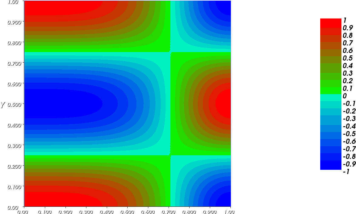
(a) data $z$

(b) estimated $u$

(c) estimated $a$

Figure 1: Reconstruction with no noise for $h=0.0176777$, $\kappa=\varepsilon=0.0001$ by OLS approach.

(a) data $z$

(b) estimated $u$

(c) estimated $a$

Figure 2: Reconstruction with no noise for $h=0.0176777$, $\kappa=0.01$, $\varepsilon=0.0001$ by MOLS approach.

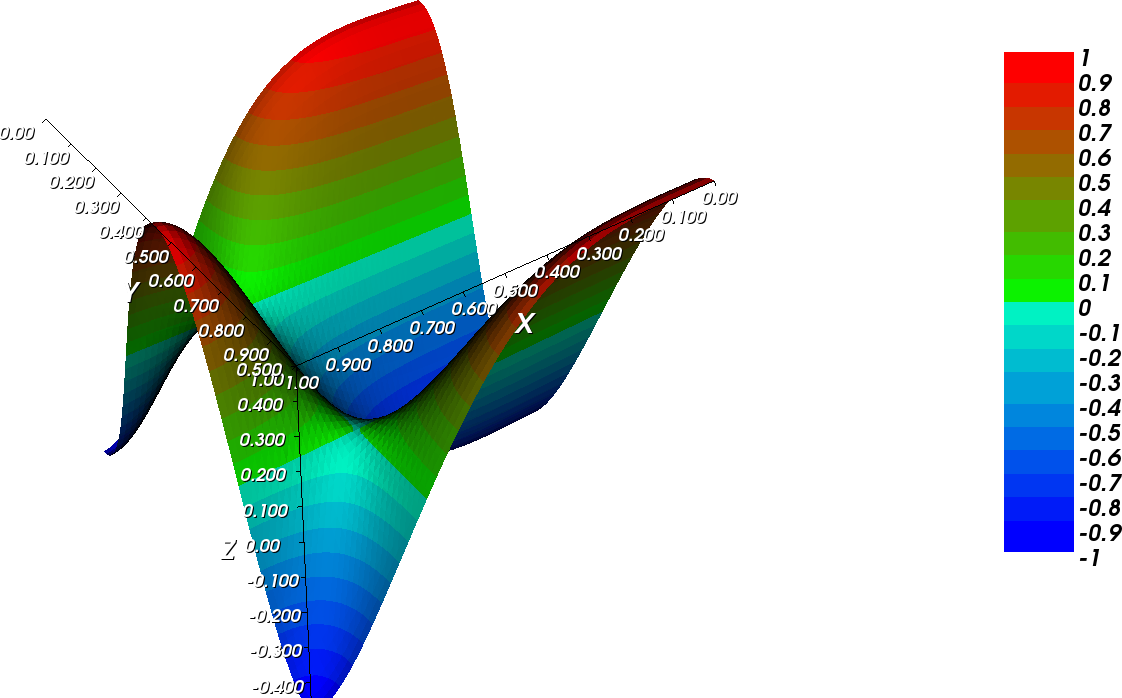
(a) data $z$

(b) estimated $u$

(c) estimated $a$

Figure 3: Failed reconstruction for $h=0.0235702$, $\kappa=0.0001$,$\varepsilon=0$ by the OLS approach.

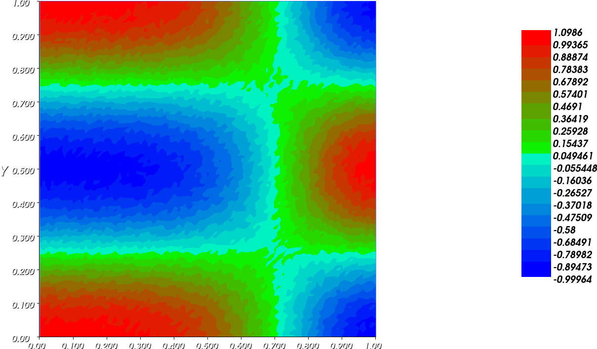
(a) data $z$

(b) estimated $u$

(c) estimated $a$

Figure 4: Reconstruction for $h=0.0176777$, $\kappa=\varepsilon=0.0001$, and noise level $\delta_{n}=0.1$ by the OLS approach.

7 Concluding Remarks

We explored the inverse problem of parameter identification in non-elliptic variational problems by posing optimization problems using the OLS and the MOLS functionals. We regularized the underlying non-elliptic variational problem and studied the features of the regularized parameter-to-solution map. For the set-valued parameter-to-solution map, we relied on the notion of the first-order and the second-order contingent derivatives. To the best of our knowledge, this is the first work where tools from set-valued optimization have been employed to assist the study of inverse problems of parameter identification. It would be of interest to explore what derivatives of set-valued maps are most convenient for this kind of research. Detailed numerical experimentation, taking into account the data perturbation, is of paramount importance and will be done in future work. An extension of the present approach to inverse problems in noncoercive variational inequalities also seems to be a promising topic to explore.

References

- [1] Robert Acar “Identification of the coefficient in elliptic equations” In SIAM J. Control Optim. 31.5, 1993, pp. 1221–1244 DOI: 10.1137/0331058
- [2] Habib Ammari, Pierre Garapon and François Jouve “Separation of scales in elasticity imaging: a numerical study” In J. Comput. Math. 28.3, 2010, pp. 354–370 DOI: 10.4208/jcm.2009.12-m1001
- [3] Claudio Baiocchi, Fabio Gastaldi and Franco Tomarelli “Some existence results on noncoercive variational inequalities” In Ann. Scuola Norm. Sup. Pisa Cl. Sci. (4) 13.4, 1986, pp. 617–659 URL: http://www.numdam.org/item?id=ASNSP_1986_4_13_4_617_0
- [4] Pavel Bochev and R.. Lehoucq “On the finite element solution of the pure Neumann problem” In SIAM Rev. 47.1, 2005, pp. 50–66 DOI: 10.1137/S0036144503426074
- [5] Christian Boehm and Michael Ulbrich “A semismooth Newton-CG method for constrained parameter identification in seismic tomography” In SIAM J. Sci. Comput. 37.5, 2015, pp. S334–S364 DOI: 10.1137/140968331
- [6] R. Boiger and B. Kaltenbacher “An online parameter identification method for time dependent partial differential equations” In Inverse Problems 32.4, 2016, pp. 045006\bibrangessep28 DOI: 10.1088/0266-5611/32/4/045006
- [7] J. Borwein “Weak tangent cones and optimization in a Banach space” In SIAM J. Control Optimization 16.3, 1978, pp. 512–522 DOI: 10.1137/0316034
- [8] J. Borwein and R. O’Brien “Tangent cones and convexity” In Canad. Math. Bull. 19.3, 1976, pp. 257–261 DOI: 10.4153/CMB-1976-040-x
- [9] M. Cho et al. “First-order and second-order adjoint methods for the inverse problem of identifying non-linear parameters in PDEs” In Industrial Mathematics and Complex Systems: Emerging Mathematical Models, Methods and Algorithms Springer Singapore, 2017, pp. 147–163 DOI: 10.1007/978-981-10-3758-0_9
- [10] Christian Clason “L∞ fitting for inverse problems with uniform noise” In Inverse Problems 28.10, 2012, pp. 104007 DOI: 10.1088/0266-5611/28/10/104007
- [11] E. Crossen et al. “An equation error approach for the elasticity imaging inverse problem for predicting tumor location” In Comput. Math. Appl. 67.1, 2014, pp. 122–135 DOI: 10.1016/j.camwa.2013.10.006
- [12] Xiaoxia Dai “Finite element approximation of the pure Neumann problem using the iterative penalty method” In Appl. Math. Comput. 186.2, 2007, pp. 1367–1373 DOI: 10.1016/j.amc.2006.07.148
- [13] R.. Evstigneev, M.. Medvedik and Yu.. Smirnov “Inverse problem of determining parameters of inhomogeneity of a body from acoustic field measurements” In Comput. Math. Math. Phys. 56.3, 2016, pp. 483–490 DOI: 10.1134/S0965542516030040
- [14] Amir Gholami, Andreas Mang and George Biros “An inverse problem formulation for parameter estimation of a reaction-diffusion model of low grade gliomas” In J. Math. Biol. 72.1-2, 2016, pp. 409–433 DOI: 10.1007/s00285-015-0888-x
- [15] M.. Gockenbach, B. Jadamba and A.. Khan “Numerical estimation of discontinuous coefficients by the method of equation error” In Int. J. Math. Comput. Sci. 1.3, 2006, pp. 343–359
- [16] M.. Gockenbach, B. Jadamba and A.. Khan “Equation error approach for elliptic inverse problems with an application to the identification of Lamé parameters” In Inverse Probl. Sci. Eng. 16.3, 2008, pp. 349–367 DOI: 10.1080/17415970701602580
- [17] Mark S. Gockenbach et al. “Proximal methods for the elastography inverse problem of tumor identification using an equation error approach” In Advances in Variational and Hemivariational Inequalities: Theory, Numerical Analysis, and Applications 33, Adv. Mech. Math. Springer, Cham, 2015, pp. 173–197 DOI: 10.1007/978-3-319-14490-0_7
- [18] Mark S. Gockenbach and Akhtar A. Khan “Identification of Lamé parameters in linear elasticity: a fixed point approach” In J. Ind. Manag. Optim. 1.4, 2005, pp. 487–497 DOI: 10.3934/jimo.2005.1.487
- [19] Mark S. Gockenbach and Akhtar A. Khan “An abstract framework for elliptic inverse problems: I. An output least-squares approach” In Math. Mech. Solids 12.3, 2007, pp. 259–276 DOI: 10.1177/1081286505055758
- [20] Mark S. Gockenbach and Akhtar A. Khan “An abstract framework for elliptic inverse problems: II. An augmented Lagrangian approach” In Math. Mech. Solids 14.6, 2009, pp. 517–539 DOI: 10.1177/1081286507087150
- [21] D. Goeleven “Noncoercive Variational Problems and Related Results” 357, Pitman Research Notes in Mathematics Series Longman, Harlow, 1996
- [22] Shyamal Guchhait and Biswanath Banerjee “Constitutive error based material parameter estimation procedure for hyperelastic material” In Comput. Methods Appl. Mech. Engrg. 297, 2015, pp. 455–475 DOI: 10.1016/j.cma.2015.09.012
- [23] William Hager, Cuong Ngo, Maryam Yashtini and Hong-Chao Zhang “An alternating direction approximate Newton algorithm for ill-conditioned inverse problems with application to parallel MRI” In J. Oper. Res. Soc. China 3.2, 2015, pp. 139–162 DOI: 10.1007/s40305-015-0078-y
- [24] Frédéric Hecht “New development in FreeFem++” In Journal of Numerical Mathematics 20.3-4 De Gruyter, 2012, pp. 251–266 DOI: 10.1515/jnum-2012-0013
- [25] B. Jadamba, A.. Khan, A. Oberai and M. Sama “First-order and second-order adjoint methods for parameter identification problems with an application to the elasticity imaging inverse problem” In Inverse Problems in Science and Engineering, 2017, pp. 1–20 DOI: 10.1080/17415977.2017.1289195
- [26] B. Jadamba et al. “A new convex inversion framework for parameter identification in saddle point problems with an application to the elasticity imaging inverse problem of predicting tumor location” In SIAM J. Appl. Math. 74.5, 2014, pp. 1486–1510 DOI: 10.1137/130928261
- [27] Baasansuren Jadamba, Akhtar A. Khan, Miguel Sama and Christiane Tammer “On convex modified output least-squares for elliptic inverse problems: stability, regularization, applications, and numerics” In Optimization 66.6, 2017, pp. 983–1012 DOI: 10.1080/02331934.2017.1316270
- [28] Mohammad F. Al-Jamal and Mark S. Gockenbach “Stability and error estimates for an equation error method for elliptic equations” In Inverse Problems 28.9, 2012, pp. 095006\bibrangessep15 DOI: 10.1088/0266-5611/28/9/095006
- [29] Tommi Kärkkäinen “An equation error method to recover diffusion from the distributed observation” In Inverse Problems 13.4, 1997, pp. 1033–1051 DOI: 10.1088/0266-5611/13/4/009
- [30] Akhtar A. Khan and Dumitru Motreanu “Inverse problems for quasi-variational inequalities” In J. Global Optim. 70.2, 2018, pp. 401–411 DOI: 10.1007/s10898-017-0597-7
- [31] Akhtar A. Khan, Christiane Tammer and Constantin Zalinescu “Regularization of quasi-variational inequalities” In Optimization 64.8, 2015, pp. 1703–1724 DOI: 10.1080/02331934.2015.1028935
- [32] Akhtar A. Khan, Christiane Tammer and Constantin Zalinescu “Set-Valued Optimization” Springer, Heidelberg, 2015 DOI: 10.1007/978-3-642-54265-7
- [33] Stefan Kindermann, Lawrence D. Mutimbu and Elena Resmerita “A numerical study of heuristic parameter choice rules for total variation regularization” In J. Inverse Ill-Posed Probl. 22.1, 2014, pp. 63–94 DOI: 10.1515/jip-2012-0074
- [34] Clemens Kirisits, Christiane Pöschl, Elena Resmerita and Otmar Scherzer “Finite-dimensional approximation of convex regularization via hexagonal pixel grids” In Appl. Anal. 94.3, 2015, pp. 612–636 DOI: 10.1080/00036811.2014.958998
- [35] Ian Knowles “Parameter identification for elliptic problems” In J. Comput. Appl. Math. 131.1-2, 2001, pp. 175–194 DOI: 10.1016/S0377-0427(00)00275-2
- [36] Peter Kuchment and Dustin Steinhauer “Stabilizing inverse problems by internal data. II: Non-local internal data and generic linearized uniqueness” In Anal. Math. Phys. 5.4, 2015, pp. 391–425 DOI: 10.1007/s13324-015-0104-6
- [37] Tao Liu “A wavelet multiscale-homotopy method for the parameter identification problem of partial differential equations” In Comput. Math. Appl. 71.7, 2016, pp. 1519–1523 DOI: 10.1016/j.camwa.2016.02.036
- [38] S. Manservisi and M. Gunzburger “A variational inequality formulation of an inverse elasticity problem” In Appl. Numer. Math. 34.1, 2000, pp. 99–126 DOI: 10.1016/S0168-9274(99)00042-2
- [39] M.. Nashed and O. Scherzer “Least squares and bounded variation regularization with nondifferentiable functionals” In Numer. Funct. Anal. Optim. 19.7-8, 1998, pp. 873–901 DOI: 10.1080/01630569808816863
- [40] Andreas Neubauer et al. “Improved and extended results for enhanced convergence rates of Tikhonov regularization in Banach spaces” In Appl. Anal. 89.11, 2010, pp. 1729–1743 DOI: 10.1080/00036810903517597
- [41] Doug Ward “Calculus for parabolic second-order derivatives” In Set-Valued Anal. 1.3, 1993, pp. 213–246 DOI: 10.1007/BF01027635