Graphene ground states

Abstract.

Graphene is locally two-dimensional but not flat. Nanoscale ripples appear in suspended samples and rolling-up often occurs when boundaries are not fixed. We address this variety of graphene geometries by classifying all ground-state deformations of the hexagonal lattice with respect to configurational energies including two- and three-body terms. As a consequence, we prove that all ground-state deformations are either periodic in one direction, as in the case of ripples, or rolled up, as in the case of nanotubes.

1. Introduction

Graphene is a one-atom thick layer of carbon atoms arranged in a regular hexagonal lattice. Its serendipitous discovery in 2005 sparkled research on two-dimensional materials systems. This new branch of Materials Science exponentially developed in the last years. An impressive variety of new low-dimensional systems has been presented and their potential for innovative applications, especially in optoelectronics, is currently strongly investigated [10].

The lower-dimensionality of graphene is at the basis of its amazing mechanical, optical, and electronic properties. On the other hand, the classical Mermin-Wagner Theorem [15, 20, 21] excludes the possibility of realizing truly two-dimensional systems at finite temperature. Indeed, observations on suspended samples seem to indicate that graphene is generally not exactly flat but gently rippled [22]. Wavy patterns on the scale of approximately one hundred atom spacings have been computationally investigated [9] and are considered to be responsible for the stabilization of graphene at finite temperature. Nonplanarity is expected even in the zero-temperature limit, due to quantum fluctuations [8]. The Reader is referred to the recent survey [5] for an overview of ripple-formation mechanisms and possible applications. On the other hand, free graphene samples in absence of support have the tendency to roll-up in tube-like structures [14].

The phenomenon of rippling and rolling-up in graphene is here tackled from the molecular-mechanical viewpoint. The actual configuration of a graphene sheet is identified with a three-dimensional deformation of the ideal hexagonal lattice. To each deformation we associate a configurational energy which takes nearest-neighbor and next-to-nearest-neighbor two-body interactions [1, 24, 25] into account and favors locally the specific bonding mode in graphene.

Our main result is a complete classification of ground-state deformations. We show that such ground states are locally not flat, as specific nonplanar optimal configurations ensue. In particular, two different optimal configurations for single hexagonal cells are identified. Geometric compatibility forces these optimal cells to combine in specific patterns in order to give rise to global deformations. This fact allows us to classify ground states, which correspond either to rippled or to rolled-up structures, see Theorem 5.1.

Before closing this introduction, let us review the literature on the mathematical modeling of graphene via Molecular Mechanics. The first global-minimality result for graphene in two dimensions has to be traced back to E & Li [6] who investigate the so-called thermodynamic limit as the number of atoms tends to infinity. Their result corresponds to an extension of the seminal theory by Theil [26] to three-body interaction energies favoring $2\pi/3$ bond angles. More recently, Farmer, Esedoḡlu, & Smereka [7] obtained an analogous result by assuming the three-body energy term to favor $\pi$ bond angles, which calls for the minimality of graphene among frustrated configurations.

In case of a finite number of atoms in two dimensions, graphene patches are identified as the only ground states in [19] and are characterized in terms of a discrete isoperimetric inequality in [4]. The emergence of a hexagonal Wulff shape as the number of atoms increases can be also quantitatively checked [4].

If one allows the configuration to be three-dimensional, flat graphene is no more expected to be a ground state [19]. By reducing to nearest-neighbor interactions, it can nonetheless be checked to be a local minimizer, under specific assumptions on the interaction potentials [23]. This stability analysis allows to tackle other carbon nanostructures as well, including nanotubes [11, 17, 18], fullerenes [12, 23], diamond [23], carbyne stratified configurations [16].

As concerns rippling, one has to mention the recent paper [3] where the Gaussian stiffness of graphene, namely its tendency to favor non-null Gaussian-curved configurations, is investigated via a discrete-to-continuum procedure. The aim there is to obtain an analytical expression for the Gaussian stiffness by focusing on a specific choice of the functional. In contrast, our focus is here on energetics and global geometries of ground states under general qualitative assumptions on the configurational energy.

The occurrence of nonflat and rolled-up ground states can be avoided by additionally imposing periodic boundary conditions. Experimentally, this corresponds to clamp the edges of a suspended graphene sample. In this case, by extending the energy to include third-neighbor interactions, we prove in the companion paper [13] that some specific optimal ripple length can be identified, independently of the sample size. This provides an analytical validation to the computational findings in [9].

2. Energy

The focus of this paper is on global minimization in three dimensions. We restrict the class of admissible configurations to deformations $y:H\to{\mathbb{R}}^{3}$ of the hexagonal lattice

$$H =\{sa+tb+rc\;:\;s,\,t\in\mathbb{Z},\,r=0,1\}$$

where $a=(3/2,\sqrt{3}/2)$, $b=(0,\sqrt{3})$, and $c=(1,0)$. In particular, the reference configuration as well as all atom coordinations (neighbors) are kept fixed. We call $a$, $b$, and $a-b$ coordinate directions of $H$ and term hexagonal graph the graph connecting all first neighbors in $H$. A reference cell is any $\{x_{1},\dots,x_{6}\}$ corresponding to a simple cycle in the hexagonal graph and we call cell its image $\{y_{1},\dots,y_{6}\}$ through $y$, namely $y_{i}=y(x_{i})$. The labeling of the atoms in each reference cell is always meant to be arranged counterclockwise with $x_{1}=na+mb$ to be such that $n+m$ is minimal in the reference cell, see Figure 1.

Figure 1. The reference cell $\{x_{1},\dots,x_{6}\}$ (left) and the cell $\{y_{1},\dots,y_{6}\}$ (right).

The cell energy of the cell $\{y_{1},\dots,y_{6}\}$ is given by

$$E_{\rm cell}(y_{1},\dots,y_{6})=\frac{1}{2}\sum_{i=1}^{6}v_{2}(|y_{i}-y_{i-1}|)+\sum_{i=1}^{6}v_{2}(|y_{i}-y_{i-2}|)+\sum_{i=1}^{6}v_{3}(\theta_{i}),$$

where sums in the indices are meant modulo $6$ throughout. The first term corresponds to nearest-neighbors and the second term to next-to-nearest-neighbors. The factor $1/2$ reflects the fact that each segment $\{y_{i+1},y_{i}\}$, called bond in the following, is contained in two adjacent hexagonal cells. With $\theta_{i}$ we indicate the bond angle at $y_{i}$ formed by the segments $\{y_{i+1},y_{i}\}$ and $\{y_{i-1},y_{i}\}$ which is less or equal to $\pi$.

We assume that the two-body interaction potential $v_{2}:{\mathbb{R}}^{+}\to[-1,\infty)$ attains its minimum value only at $1$ with $v_{2}(1)=-1$. Moreover, we suppose that $v_{2}$ is continuous and decreasing on $(0,1)$ (i.e., short-range repulsive) and $v_{2}$ increasing on $[1,\infty)$ (long-range attractive). Furthermore, we suppose that $v_{2}$ is differentiable in $(5/4,\sqrt{3}]$ with $v_{2}^{\prime}>0$. The three-body interaction density $v_{3}:[0,\pi]\to[0,\infty)$ is assumed to be continuous and to attain the minimum value $0$ only at $2\pi/3$ where it is differentiable. These basic assumptions correspond to the fact that $sp2$ covalent bonds in carbon are characterized by some reference bond length, here normalized to 1, and a reference bond angle of amplitude $2\pi/3$ [2]. Note that $E_{\rm cell}$ has a bounded sublevel (among cells with barycenter zero) and is continuous. As such, it admits minimizers, which we call optimal cells. These will be characterized in Proposition 4.1. For a fine characterization of the minimizers, some additional qualification on $v_{2}$ and $v_{3}$ will be needed, see conditions (2.1)-(2.4) below.

We identify the deformation $y:H\to{\mathbb{R}}^{3}$ with the collection of its cells. Furthermore, cells are identified via the inverse of $y$ to their reference cells and these are labeled in terms of their barycenters. Indeed, barycenters of reference cells form the triangular lattice

$$T =(1/2,\sqrt{3}/2)+\{sa+tb\;:\;s,\,t\in\mathbb{Z}\}.$$

We will hence equivalently indicate cells as $\{y_{1},\dots,y_{6}\}\in({\mathbb{R}}^{3})^{6}$ or $(s,t)\in\mathbb{Z}^{2}$, where $sa+tb$ is the barycenter of the corresponding reference cell $\{x_{1},\dots,x_{6}\}$.

The energy of the deformation $y:H\to{\mathbb{R}}^{3}$ is then defined as

$$E(y)=\sup_{m\in\mathbb{N}}\left(\frac{1}{\#(T\cap B_{m})}\sum_{(s,t)\in T\cap B_{m}}E_{\rm cell}(s,t)\right)$$

where $B_{m}\subset{\mathbb{R}}^{2}$ is the ball centered at $0$ having radius $m$. A deformation is called a ground state if it minimizes the energy $E$. Note that $E$ corresponds to the supremum of cell-energy densities on bounded sets of cells. This immediately entails the following.

Proposition 2.1 (Only optimal cells).

A deformation is a ground state if and only if all its cells are optimal.

Proof.

By letting $E^{*}=\min E_{\rm cell}$, we readily check that $E\geq E^{*}$. If all cells are optimal, we have $E=E^{*}$ and the deformation is a ground state. On the other hand, let $E=E^{*}$ and assume by contradiction that the cell $(s,t)\in T\cap B_{m}$ is not optimal. Then,

$$E\geq\frac{1}{\#(T\cap B_{m})}\sum_{(s,t)\in T\cap B_{m}}E_{\rm cell}(s,t)>E^{*},$$

contradicting minimality. ∎

In the following, some quantitative specifications on the interaction densities $v_{2}$ and $v_{3}$ will be assumed. These are intended to ensure that optimal cells indeed have a hexagonal-like shape. In particular, we will ask for a small parameter $0<\delta\leq 0.2$ such that

$$v_{2}(1-\delta)>11+12v_{2}(\sqrt{3}),$$ (2.1)

$$v_{2}(1+\delta)>-1+12v_{2}(\sqrt{3})-12v_{2}(\sqrt{3}(1-\delta)^{2}),$$ (2.2)

$$v_{3}(\theta)>6+6v_{2}(\sqrt{3})\quad\text{if}\ \ |\theta-2\pi/3|\geq\delta,$$ (2.3)

$$(\ell_{1},\ell_{2},\theta)\mapsto\frac{1}{4}v_{2}(\ell_{1})+\frac{1}{4}v_{2}(\ell_{2})+v_{2}\big{(}(\ell_{1}^{2}+\ell_{2}^{2}-2\ell_{1}\ell_{2}\cos\theta)^{1/2}\big{)}+v_{3}(\theta)$$

$$\ \ \ \ \ \ \ \ \ \ \ \ \ \ \ \ \text{is strictly convex for}\ \ |\ell_{1}-1|<\delta,\ |\ell_{2}-1|<\delta,\ |\theta-2\pi/3|<\delta.$$ (2.4)

Properties (2.1)-(2.2) entail that first-neighbor bond lengths range between $1-\delta$ and $1+\delta$ (note that $\sqrt{3}$ is the second-neighbor distance in $H$), whereas (2.3) ensures that the bond angles of the optimal cell are $\delta$-close to $2\pi/3$. Eventually, assumption (2.4) yields that the contribution of first-neighbors is strong enough to entail the symmetry of the optimal cell, see Proposition 3.1.

Assumptions (2.1)-(2.4) will be tacitly assumed in the rest of the paper. Note that these are compatible with a choice of densities $v_{2}$ and $v_{3}$ growing sufficiently fast out of their minima and $v_{2}$ is sufficiently flat but increasing around $\sqrt{3}$. In particular, the quantitative assumptions on $v_{2}$ introduced by Theil [26] (see also [6, 7]) imply (2.1)-(2.2). As a matter of illustration, one can choose the Lennard-Jones-like potential $v_{2}$ and the Tersoff term $v_{3}$ [25]

$$v_{2}(\ell)=(a-1)\,\ell^{-a}-a\,\ell^{-a+1}\qquad v_{3}(\theta)=\kappa(1/2+\cos\theta)^{2}$$

with $\kappa$ large enough (note that $v_{2}$ has minimum $-1$ in $\ell=1$). For instance, one can choose $a=18$, $\kappa=600$, and $\delta=0.12$.

3. Optimal cells

The aim of this section is to prove that optimal cells have specific bonds and angles. Such a property will be used in Section 4.1 in order to characterize completely optimal cells.

Proposition 3.1 (Bonds and angles of optimal cells).

All bonds of an optimal cell have length $\ell^{*}\leq 1$ and all angles have amplitude $\theta^{*}<2\pi/3$, where $\ell^{*}$ and $\theta^{*}$ are uniquely determined in terms of the energy.

Proof.

Recall assumptions (2.1)-(2.4) and let $\{y_{1},\dots,y_{6}\}$ be an optimal cell. We first show that $|y_{j}-y_{j-1}|\in(1-\delta,1+\delta)$ and $\theta_{j}\in(2\pi/3-\delta,2\pi/3+\delta)$ for all $j=1,\dots,6$.

In case $|y_{j}-y_{j-1}|\leq 1-\delta$ for some $j=1,\dots,6$, one has that

$$E_{\rm cell}(y_{1},\dots,y_{6}) =\frac{1}{2}\sum_{i=1}^{6}v_{2}(|y_{i}-y_{i-1}|)+\sum_{i=1}^{6}v_{2}(|y_{i}-y_{i-2}|)+\sum_{i=1}^{6}v_{3}(\theta_{i})$$

$$\stackrel{{\scriptstyle\rm(a)}}{{\geq}}\frac{1}{2}v_{2}(1-\delta)+\frac{1}{2}\sum_{i\not=j}v_{2}(|y_{i}-y_{i-1}|)+\sum_{i=1}^{6}v_{2}(|y_{i}-y_{i-2}|)+\sum_{i=1}^{6}v_{3}(\theta_{i})$$

$$\stackrel{{\scriptstyle\rm(b)}}{{\geq}}\frac{1}{2}v_{2}(1-\delta)-\frac{5}{2}-6+\sum_{i=1}^{6}v_{3}(\theta_{i})$$

$$\stackrel{{\scriptstyle\eqref{minimal}}}{{>}}-3+6v_{2}(\sqrt{3})=E_{\rm cell}(x_{1},\dots,x_{6}),$$

where we have used that (a) $v_{2}$ is decreasing in $(0,1)$ and (b) $v_{2}\geq-1$. This contradicts optimality as the reference cell $\{x_{1},\dots,x_{6}\}$, i.e. the identity deformation, would have strictly lower energy. We conclude that all first-neighbor bonds have to have at least length $1-\delta$.

Assume now that some bond angle $\theta_{j}$ is such that $|\theta_{j}-2\pi/3|\geq\delta$. Then

$$E_{\rm cell}(y_{1},\dots,y_{6}) =\frac{1}{2}\sum_{i=1}^{6}v_{2}(|y_{i}-y_{i-1}|)+\sum_{i=1}^{6}v_{2}(|y_{i}-y_{i-2}|)+\sum_{i=1}^{6}v_{3}(\theta_{i})$$

$$\geq-9+v_{3}(\theta_{j})\stackrel{{\scriptstyle\eqref{angle}}}{{>}}-3+6v_{2}(\sqrt{3})=E_{\rm cell}(x_{1},\dots,x_{6})$$

which again contradicts optimality. We have hence proved that all bond angles $\theta$ necessarily satisfy $|\theta-2\pi/3|<\delta$.

Basic trigonometry together with the least size of the bond lengths and bond angles ensures that second-neighbor bonds have at least length

$$2(1-\delta)\sin(\pi/3-\delta/2)=2(1-\delta)\left(\frac{\sqrt{3}}{2}\cos(\delta/2)-\frac{1}{2}\sin(\delta/2)\right)>\sqrt{3}(1-\delta)^{2}>1$$ (3.1)

where we also used that $0<\delta\leq 0.2$. Assume now that $|y_{j}-y_{j-1}|>1+\delta$ for some $j=1,\dots,6$. We have that

$$E_{\rm cell}(y_{1},\dots,y_{6}) =\frac{1}{2}\sum_{i=1}^{6}v_{2}(|y_{i}-y_{i-1}|)+\sum_{i=1}^{6}v_{2}(|y_{i}-y_{i-2}|)+\sum_{i=1}^{6}v_{3}(\theta_{i})$$

$$\stackrel{{\scriptstyle\rm(c)}}{{\geq}}\frac{1}{2}v_{2}(1+\delta)-\frac{5}{2}+6v_{2}(\sqrt{3}(1-\delta)^{2})\stackrel{{\scriptstyle\eqref{maximal}}}{{>}}-3+6v_{2}(\sqrt{3})=E_{\rm cell}(x_{1},\dots,x_{6}),$$

where we have used in (c) that all second-neighbor bonds have length at least $\sqrt{3}(1-\delta)^{2}$, see (3.1), and $v_{2}$ is increasing in $(1,\infty)$. The latter inequality once again contradicts optimality and we conclude that all first-neighbor bond lengths are at most $1+\delta$.

We have proved that if $\{y_{1},\dots,y_{6}\}$ is optimal, first-neighbor bond lengths $\ell_{i}=|y_{i}-y_{i-1}|$ lie in $(1-\delta,1+\delta)$ and bond angles $\theta_{i}$ lie in $(2\pi/3-\delta,2\pi/3+\delta)$. We can now decompose the cell energy $E_{\rm cell}$ and use the convexity assumption (2.4) in order to get that

$$E_{\rm cell}(y_{1},\dots,y_{6}) =\sum_{i=1}^{6}\left(\frac{1}{4}v_{2}(\ell_{i})+\frac{1}{4}v_{2}(\ell_{i+1})+v_{2}((\ell_{i}^{2}+\ell_{i+1}^{2}-2\ell_{i}\ell_{i+1}\cos\theta_{i})^{1/2})+v_{3}(\theta_{i})\right)$$

$$\geq 6\left(\frac{1}{2}v_{2}(\ell^{*})+v_{2}(\sqrt{2}\ell^{*}(1-\cos\theta^{*})^{1/2})+v_{3}(\theta^{*})\right)$$ (3.2)

where

$$\ell^{*}=\frac{1}{6}(\ell_{1}+\dots+\ell_{6}),\quad\theta^{*}=\frac{1}{6}(\theta_{1}+\dots+\theta_{6}).$$

As the inequality in (3) is strict whenever $\ell_{i}\not=\ell^{*}$ or $\theta_{i}\not=\theta^{*}$ for some $i=1,\dots,6$, all bonds of an optimal cell have length $\ell^{*}$ and all angles have amplitude $\theta^{*}$. It remains to check that $\ell^{*}\leq 1$ and $\theta^{*}<2\pi/3$. First, if we had $\ell^{*}>1$, one could reduce the energy in (3) by reducing $\ell^{*}$ noting that $v_{2}$ is increasing in $(1,\infty)$ and recalling (3.1). This, however, would again contradict optimality. On the other hand, we have that

$$6\theta^{*}=\theta_{1}+\dots+\theta_{6}\leq 4\pi$$

as $4\pi$ is the sum of the internal angles of a planar hexagon. In particular, the equality holds iff $\{y_{1},\dots,y_{6}\}$ is planar. Hence, we have that $\theta^{*}\leq 2\pi/3$. However, we can exclude that $\theta^{*}=2\pi/3$ for in this case all second neighbors would have distance $\sqrt{3}\ell^{*}\in\sqrt{3}(1-\delta,1]\subset\sqrt{3}(0.8,1]\subset(5/4,\sqrt{3}]$. As $v_{2}^{\prime}(\sqrt{3}\ell^{*})>0$ and $v_{3}^{\prime}(2\pi/3)=0$, one would then strictly lower the energy in (3) by reducing $\theta^{*}$. ∎

Before closing this section let us comment on the importance of the condition $v_{2}^{\prime}>0$ in a left neighborhood of $\sqrt{3}$. This has been used in the proof of Proposition 3.1 in order to check that $\theta^{*}$ is strictly smaller than $2\pi/3$. Indeed, if $v_{2}^{\prime}$ were flat in a neighborhood of $\sqrt{3}$, which would correspond to the case of purely first-neighbor interactions, one would find $\theta^{*}=2\pi/3$, $\ell^{*}=1$ [23], and the optimal cell would be planar. Correspondingly, the only ground state would be the hexagonal lattice $H$.

4. The $Z$ and the $C$ cells

In the previous section we have proved that all cells of a ground state have all bonds of length $\ell^{*}$ and all bond angles $\theta^{*}$. The aim of this section is to check that such properties determine the cell (up to isometries). More precisely, Proposition 4.1 below states that exactly two geometries are possible: the $Z$ cell and the $C$ cell. This naming refers to the cell shape, see Figure 2, and has been inspired by [3], where this nomenclature is however used for triplets of adjacent bonds.

Figure 2. The $Z$ cell (left) and $C$ cell (right), prospective views (top) and side views (bottom). The normal vector $n_{0}$ to the darkened triangle $\{y_{1},y_{3},y_{5}\}$, its center $y_{0}$, and the angles $\alpha_{*}$, $\alpha_{**}$ play an important role in the proof of Proposition 4.1. We will refer to the angle $\beta$ in Section 5.

The $Z$ and the $C$ cell are specified as follows

$$Z =\{(-\ell^{*}/2,-v,0),\,(\ell^{*}/2,-v,0),\,(\ell,0,h),\,(\ell^{*}/2,v,0)),\,(-\ell^{*}/2,v,0),\,(-\ell,0,-h)\},$$

$$C =\{(-\ell^{*}/2,-v,0),\,(\ell^{*}/2,-v,0),\,(\ell,0,h),\,(\ell^{*}/2,v,0)),\,(-\ell^{*}/2,v,0),\,(-\ell,0,h)\}$$

where $v$, $\ell$, and $h$ are given by

$$v=\ell^{*}\left(\frac{1}{2}-\frac{1}{2}\cos\theta^{*}\right)^{1/2},\quad\ell=\frac{\ell^{*}}{2}-\ell^{*}\cos\theta^{*},\quad h=\ell^{*}\left(\frac{1}{2}+\frac{1}{2}\cos\theta^{*}-\cos^{2}\theta^{*}\right)^{1/2}.$$ (4.1)

These explicit values can be obtained by elementary (yet tedious) trigonometry. Note that if $\theta^{*}$ were $2\pi/3$ (which is not), the above formulas would give $v=(\sqrt{3}/2)\ell^{*}$, $\ell=\ell^{*}$, and $h=0$, corresponding indeed to the flat hexagonal lattice of spacing $\ell^{*}$.

A remarkable property of the $Z$ and the $C$ cell is that they have a pair of parallel bonds which define a plane with normal $e_{3}$ containing four out of six atoms of the cells. By considering the two semispaces divided by such plane, the $Z$ and the $C$ cell are easily distinguishable as the two off-planar atoms of $Z$ belong to two distinct semispaces, whereas those of $C$ belong to the same semispace. Both cells are symmetric with respect to the $(e_{1},e_{3})$ plane. In addition, $Z$ is central symmetric as well as invariant by $2\pi/3$ and $4\pi/3$ rotations about the axis with direction $(y_{3}{-}y_{1})\wedge(y_{5}{-}y_{1})$ (i.e., direction of $n_{0}$ in Figure 2).

The main result of this section is the following characterization.

Proposition 4.1 ($C$ and $Z$ cells).

Optimal cells are either $C$ or $Z$.

Proof.

As bonds and bond angles of an optimal cell $Y=\{y_{1},\dots,y_{6}\}$ are all equal, the distance of each pair of second neighbors is equal as well. In particular, the three atoms $y_{1}$, $y_{3}$, and $y_{5}$ are the vertices of an equilateral triangle and determine a plane, which we indicate with $A$, see Figure 2. Fix an orientation on $A$ via the unit vector $n_{0}$ with direction $(y_{3}{-}y_{1})\wedge(y_{5}{-}y_{1})$ and indicate with $\alpha_{2}$, $\alpha_{4}$, and $\alpha_{6}$ the incidence angles with $A$ of the planes $A_{2}$, $A_{4}$, and $A_{6}$ containing $\{y_{1},y_{2},y_{3}\}$, $\{y_{3},y_{4},y_{5}\}$, and $\{y_{5},y_{6},y_{1}\}$, respectively. More precisely, let $n_{2}$, $n_{4}$, and $n_{6}$ be the unit vectors with directions $(y_{3}{-}y_{2})\wedge(y_{1}{-}y_{2})$, $(y_{5}{-}y_{4})\wedge(y_{3}{-}y_{4})$, and $(y_{1}{-}y_{6})\wedge(y_{5}{-}y_{6})$, respectively, and recall that

$$\alpha_{i}=\arccos(n_{0}\cdot n_{i})\in[0,\pi]\quad\text{for}\ \ i=2,4,6.$$

The geometry of the cell $Y$ is completely determined by the three incidence angles $\alpha_{2}$, $\alpha_{4}$, and $\alpha_{6}$ and by the sign of the products

$$p_{i}=(y_{i}{-}y_{0})\cdot n_{0}\quad\text{for}\ \ i=2,4,6$$

where we have indicated by $y_{0}$ the center of $A$, namely $y_{0}=(y_{1}+y_{3}+y_{5})/3$.

In the case of the $Z$ cell, all $p_{i}$ have the same sign and all incidence angles are all equal to

$$\alpha^{*}=\arctan\left(\frac{h}{\ell-\ell^{*}/2}\right)-\arctan\left(\frac{h}{\ell+\ell^{*}/2}\right)$$

which just depends on $\theta^{*}$, see (4.1). In particular, in the setting of Figure 2 one has that $p_{i}<0$ for $i=2,4,6$.

In case of the $C$ cell, one has that two out of three products $p_{i}$ have the same sign and the third has the opposite sign. The incidence angles $\alpha_{i}$ corresponding to the products $p_{i}$ with the same sign are $\alpha^{*}$ and that corresponding to the product with opposite sign equals

$$\alpha^{**}=\arctan\left(\frac{h}{\ell-\ell^{*}/2}\right)+\arctan\left(\frac{h}{\ell+\ell^{*}/2}\right)$$

which again depends on $\theta^{*}$ only. The setting of Figure 2 corresponds to $p_{6}>0>p_{2},\,p_{4}$ and $\alpha_{2}=\alpha_{4}=\alpha^{*}$ and $\alpha_{6}=\alpha^{**}$.

Let an optimal cell $Y=\{y_{1},\dots,y_{6}\}$ be given and define the corresponding $\alpha_{i}$ and $p_{i}$. By possibly relabeling the atoms (in such a way that neighbors remain neighbors) we can reduce ourselves to one of the following cases: (1) $p_{i}\leq 0$ for $i=2,4,6$ or (2) $p_{6}\geq 0\geq p_{2},p_{4}$. Note that these cases exhaust all possibilities, being however not mutually exclusive. The statement follows now by checking that, up to isometry, $Y=Z$ in Case (1) and $Y=C$ in Case (2).

Assume that we have $p_{i}\leq 0$, namely Case (1). Drop the constraint $\theta_{3}=\theta^{*}$ by keeping all others (all bonds have length $\ell^{*}$ and all bond angles other than $\theta_{3}$ are equal to $\theta^{*}$). This uniquely defines $\theta_{3}$ as a function of $\alpha_{6}$, namely $\theta_{3}=\theta_{3}(\alpha_{6})$. Indeed, there exists $\alpha^{*}<\alpha_{\rm max}^{*}<\pi$ such that for all $\alpha_{6}\in[0,\alpha_{\rm max}^{*}]$ one can uniquely determine $\alpha_{2}=\alpha_{4}\in[0,\pi]$ with $\theta_{1}=\theta_{5}=\theta^{*}$ by keeping $p_{2},\,p_{4}\leq 0$ and for $\alpha_{6}>\alpha_{\rm max}^{*}$ such values $\alpha_{2},\,\alpha_{4}$ do not exist. Note that the mapping $\alpha_{6}\mapsto\alpha_{2}=\alpha_{4}$ is strictly decreasing. Moreover, $\alpha_{2}(\alpha^{*})=\alpha_{4}(\alpha^{*})=\alpha^{*}$. Indeed, if this was not the case, the bond angles $\theta_{1}$ and $\theta_{5}$ would not be $\theta^{*}$. Corresponding to changes in $\alpha_{2}=\alpha_{4}$ and for $p_{2},\,p_{4}\leq 0$, the angle $\theta_{3}$ changes as well and the mapping $\alpha_{2}=\alpha_{4}\mapsto\theta_{3}$ is strictly decreasing. This entails that the composed mapping $\alpha_{6}\mapsto\theta_{3}(\alpha_{6})$ is strictly increasing. Hence, the equation $\theta_{3}(\alpha_{6})=\theta^{*}$ has a unique solution. Such solution is necessarily $\alpha_{6}=\alpha^{*}$, for this happens to be the case for $Z$. Recalling that $\alpha_{2}(\alpha^{*})=\alpha_{4}(\alpha^{*})=\alpha^{*}$, we have hence proved that $\alpha_{i}=\alpha^{*}$ for $i=2,4,6$, so that $Y$ is necessarily $Z$.

Assume now that $p_{6}\geq 0\geq p_{2},p_{4}$, namely Case (2). Drop the constraint $\theta_{3}=\theta^{*}$ by keeping all others. Let $\alpha^{**}<\alpha_{\rm max}^{**}<\pi$ be given such that for all $\alpha_{6}\in[0,\alpha_{\rm max}^{**}]$ one finds uniquely $\alpha_{2}=\alpha_{4}\in[0,\pi]$ with $\theta_{1}=\theta_{5}=\theta^{*}$ by keeping $p_{2},\,p_{4}\leq 0$ and for $\alpha_{6}>\alpha_{\rm max}^{**}$ such values $\alpha_{2},\,\alpha_{4}$ do not exist. Note that the mapping $\alpha_{6}\mapsto\alpha_{2}=\alpha_{4}$ is strictly increasing and that $\alpha_{4}(\alpha^{**})=\alpha_{6}(\alpha^{**})=\alpha^{*}$. Indeed, if this was not the case, the bond angles $\theta_{1}$ and $\theta_{5}$ would not be $\theta^{*}$. On the other hand, the mapping $\alpha_{2}=\alpha_{4}\mapsto\theta_{3}$ is strictly decreasing. Thus, the composed mapping $\alpha_{6}\mapsto\theta_{3}(\alpha_{6})$ is strictly decreasing and the equation $\theta_{3}(\alpha_{6})=\theta^{*}$ has the only solution $\alpha_{6}=\alpha^{**}$, for this corresponds to $C$. As $\alpha_{2}(\alpha^{**})=\alpha_{4}(\alpha^{**})=\alpha^{*}$, we have proved that $\alpha_{2}=\alpha_{4}=\alpha^{*}$ and $\alpha_{6}=\alpha^{**}$. In particular, $Y$ is $C$. ∎

5. Classification of ground states

Proposition 4.1 provides a local description of ground-state geometries. The purpose of this section is to move from such a local description to the global picture. This is made possible as $Z$ and $C$ cells can be arranged in three-dimensional space just in few very specific global patterns. This eventually allows us to classify ground-state deformations in Theorem 5.1.

In order to state our result, we need to introduce some finer description of cell geometries. Note indeed that Proposition 4.1 identifies optimal cells as point sets up to isometries. Here we need to specialize this identification by taking into account the indicization of the atoms as well. In particular, we say that two optimal cells $\{y_{1},\dots,y_{6}\}$ and $\{z_{1},\dots,z_{6}\}$ are of the same type if they are isomorphic via an isometry $\iota:{\mathbb{R}}^{3}\to{\mathbb{R}}^{3}$ with the property that $\iota(y_{i})=z_{i}$ for $i=1,\ldots,6$.

In order to find all possible types of optimal cells, one has to consider all permutations $\{i_{1},\dots,i_{6}\}$ of the atomic indices $\{1,\dots,6\}$ which preserve first neighbors, namely such that $|i_{k}-i_{k-1}|=1$ (the sum being modulo $6$). Such permutations are generated by the two transformations $i\to i+1$ and $i\to-i$.

As $Z$ cells as point sets are invariant under $2\pi/3$ rotations about their axis $n_{0}$ (see Figure 2) and are central symmetric, by applying such generating transformations to the atomic indices of $Z$ cells we identify exactly two equivalence classes: We say that a $Z$ cell $\{y_{1},\dots,y_{6}\}$ is of type $Z$ if it is of the same type of the $Z$ cell of Figure 2 and that it is of type $\overline{Z}$ if it is of the same type of the $Z$ cell of Figure 2 up to letting $y_{i}\to y_{-i}$. Type $Z$ cells $\{y_{1},\dots,y_{6}\}$ are transformed into type $\overline{Z}$ cells (and viceversa) both by $y_{i}\to y_{i+1}$ or $y_{i}\to y_{-i}$.

As $C$ cells are less symmetric than $Z$ cells, the type count for $C$ cells is necessarily higher. A $C$ cell $\{y_{1},\dots,y_{6}\}$ is said to be of type $C$ if it is of the same type of the $C$ cell of Figure 2 and to be of type $\overline{C}$ if it is of the same type of the $C$ cell of Figure 2 up to letting $y_{i}\to y_{-i}$. On the other hand, a $C$ cell is said to be of type $C_{\pm}$ ($\overline{C}_{\pm}$) if it is of the same type of the $C$ cell of Figure 2 up to letting $y_{i}\to y_{i\pm 1}$ ($y_{i}\to y_{-(i\pm 1)}$, respectively). Type $C$ and $C_{\pm}$ cells $\{y_{1},\dots,y_{6}\}$ are respectively transformed into type $\overline{C}$ and $\overline{C}_{\pm}$ cells by the transformation $y_{i}\to y_{-i}$.

The above provisions define a type function

$$\tau:\mathbb{Z}^{2}\to\{Z,\overline{Z},C,\overline{C},C_{+},\overline{C}_{+},C_{-},\overline{C}_{-}\}$$

which associates to each cell $(s,t)\in\mathbb{Z}^{2}$ its type $\tau(s,t)$. The cells in Figure 2 are of type $Z$ (left) and type $C$ (right). A type $\overline{Z}$ and type $\overline{C}$ cell can be visualized by taking the reflection of a type $Z$ and type $C$ cell, respectively, with respect to the plane $(e_{1},e_{3})$.

Define the center $y_{\rm c}$ of the cell by

$$y_{\rm c}=\frac{1}{4}(y_{1}+y_{2}+y_{4}+y_{5}).$$

To each bond $\{y_{i},y_{i+1}\}$ we associate a bond plane defined as the plane containing the endpoints of the bond and the center $y_{\rm c}$ of the cell, oriented by the unit vector $n$ with direction $(y_{i}{-}y_{\rm c})\wedge(y_{i+1}{-}y_{\rm c})$.

Let now the two cells $(s,t)$ and $(s^{\prime},t^{\prime})$ with centers $y_{\rm c}$ and $y_{\rm c}^{\prime}$ share the bond $\{y_{i},y_{j}\}$. We define the signed incidence angle $\gamma\in[-\pi,\pi]$ at the bond $\{y_{i},y_{j}\}$ of the corresponding bond planes as

$$\gamma=\left\{\begin{array}[]{ll}\phantom{-}\arccos(n\cdot n^{\prime})&\text{if}\ \ (y^{\prime}_{\rm c}{-}y_{\rm c})\cdot(n^{\prime}{-}n)<0\\ -\arccos(n\cdot n^{\prime})&\text{if}\ \ (y^{\prime}_{\rm c}{-}y_{\rm c})\cdot(n^{\prime}{-}n)\geq 0\end{array}\right.$$

where $n$ and $n^{\prime}$ denote the unit vectors to the bond planes in the cells $(s,t)$ and $(s^{\prime},t^{\prime})$, respectively. Note that this definition is invariant under the transformation $(s,t)\leftrightarrow(s^{\prime},t^{\prime})$ and that $|\gamma|$ is the classical incidence angle between the two bond planes.

In the following, an important role will be played by the angle (recall definitions (4.1))

$$\gamma^{*}=4\arctan(h/v)=4\arctan\left(\frac{1+\cos\theta^{*}-2\cos^{2}\theta^{*}}{1-\cos\theta^{*}}\right)^{1/2}.$$ (5.1)

Note that $\gamma^{*}/2$ is the incidence angle of the two planes containing the atoms $\{y_{1},y_{2},y_{3},y_{6}\}$ and $\{y_{3},y_{4},y_{5},y_{6}\}$ of the type $C$ cell, see Figure 2. For each cell $(s,t)$, we let $\widehat{\gamma}(s,t)$ be the signed incidence angle at the common bond between cell $(s,t)$ and cell $(s,t-1)$. This notation allows us to state our main result.

Theorem 5.1 (Classification of ground states).

A deformation is a ground state if and only if, possibly up to a reorientation of the reference lattice $H$, the type function $\tau$ takes values only in $\{Z,\overline{Z},C,\overline{C}\}$ and one of the following two cases occurs

(Zigzag roll-ups)           $\widehat{\gamma}\equiv-\gamma^{*}$ and $\tau\equiv C$ or $\,\widehat{\gamma}\equiv\gamma^{*}$ and $\tau\equiv\overline{C}$.

(Rippled structures)  $\widehat{\gamma}\equiv 0$ and $t\mapsto\tau(s,t)$ is constant for all $s\in\mathbb{Z}$,

The fact that the type function takes values exclusively in $\{Z,\overline{Z},C,\overline{C}\}$ and, in particular, values $C_{\pm}$ and $\overline{C}_{\pm}$ do not occur is due to the reorientation of the reference lattice $H$. Even without such reorientation, a statement in the spirit of Theorem 5.1 would hold. The four possible values of the type function would then be either $\{Z,\overline{Z},C,\overline{C}\}$, $\{Z,\overline{Z},C_{+},\overline{C}_{+}\}$, or $\{Z,\overline{Z},C_{-},\overline{C}_{-}\}$.

The classification of Theorem 5.1 says that exactly two families of ground states exist. In case $\widehat{\gamma}\equiv-\gamma^{*}$ and $\tau\equiv C$ (or, equivalently, $\widehat{\gamma}\equiv\gamma^{*}$ and $\tau\equiv\overline{C}$) the ground state is a rolled-up structure which is usually referred to as of zigzag type, see Figure 3.

Figure 3. Zigzag structure: $\tau\equiv C$ and $\widehat{\gamma}\equiv-\gamma^{*}$ (or, equivalently, $\tau\equiv\overline{C}$ and $\widehat{\gamma}\equiv\gamma^{*}$).

If $\gamma^{*}=\pi/m$ for some $m\in\mathbb{N}$ large enough, the configuration is a zigzag nanotube with $m$ cells on each section. Note, however, that such condition on $\gamma^{*}$ is nongeneric with respect to the choice of the energy, see (5.1). The zigzag ground-state deformation is not injective iff $k\gamma^{*}=\pi/m+2\pi j$ for some $k,\,j\in\mathbb{N}$.

The second possibility from the classification of Theorem 5.1 is that $\widehat{\gamma}\equiv 0$. In this case, the ground state corresponds to an alternation of cell types which are constant along the coordinate direction $b$. The ground state is hence uniquely determined by the sequence of types, e.g. $\{\dots,C,C,\overline{Z},Z,C,\overline{C},\dots\}$. All such sequences can in principle be considered, although some of them give rise to noninjective deformations or even self-interpenetrating structures.

The choices

$$\{\dots,C,\overline{C},C,\overline{C},C\dots\},$$

$$\{\dots,C,C,\overline{C},\overline{C},C,C,\overline{C},\overline{C},C,C\dots\},$$

$$\{\dots,C,C,C,\overline{C},\overline{C},\overline{C},C,C,C,\overline{C},\overline{C},\overline{C},C,C,C\dots\},$$

originate ripples with different wave lengths, corresponding to the different number of copies of $C$ and $\overline{C}$ in the sequence. Choices including $Z$ and $\overline{Z}$ cells can generate ripples as well, see Figure 4.

Figure 4. Examples of rippled structures for $\widehat{\gamma}\equiv 0$: $\{\dots,C,\overline{C},C,\overline{C},C\dots\}$ (left) and $\{\dots,\overline{Z},\overline{C},Z,C,\dots\}$ (right).

The constant choice $\{\dots,C,C,C,\dots\}$ gives rise to a rolled-up structure of the so-called armchair type, see Figure 5.

Figure 5. Armchair structure: $\{\dots,C,C,C,\dots\}$ for $\widehat{\gamma}\equiv 0$.

If one has that

$$\beta=\arctan\left(\frac{h}{\ell-\ell^{*}/2}\right)=\frac{\pi}{m}$$

for some $m\in\mathbb{N}$ large enough (see Figure 2 bottom right), the rippled structure $\{\dots,C,C,C,\dots\}$ closes up and we have an armchair nanotube [11, 17] with $m$ atoms on each (nonempty) section. Again, the condition on $\beta$ is nongeneric.

In the rippled case, ground states are essentially one dimensional. Indeed, the sequence of cell types is completely characterized by any section with respect to direction $b^{\perp}$ in $H$, see Figure 6. One can hence introduce an effective energy for such sections by considering cell centers as particles and favoring a specific distance between cell centers and a specific angle $\varphi^{*}$ between segments connecting neighboring cell centers. We follow this path in [13] where we show that third-neighbor interactions between cell centers and certain boundary conditions select specific optimal ripple lengths, independently of the sample size (assumed to be sufficiently large).

Note that for all $\varphi$ close to $\pi$ one can find $\theta=\theta(\varphi)$ close to $2\pi/3$ so that, by letting all bond angles of the $C$ and $\overline{C}$ cells in Figure 6 be $\theta$ (possibly being not optimal), the segments connecting cell centers form $\varphi$ angles which each other. The ground state corresponds then to $\theta=\theta^{*}$ or $\varphi=\varphi^{*}$ and one can check that

$$2\pi/3-\theta^{*}\sim(\pi-\varphi^{*})^{2}.$$

In particular, by defining $\widehat{v}_{3}(\varphi)=v_{3}(\theta(\varphi))$ (and letting $v_{3}$ be smooth in $2\pi/3$) one has that $\widehat{v}_{3}$ is minimized in $\pi$ with

$$\widehat{v}_{3}^{\prime}(\pi)=\widehat{v}_{3}^{\prime\prime}(\pi)=\widehat{v}_{3}^{\prime\prime\prime}(\pi)=0\quad\text{and}\quad\widehat{v}_{3}^{\prime\prime\prime\prime}(\pi)>0.$$ (5.2)

Figure 6. Effective description of a $b^{\perp}$ section of the rippled structure $\{\dots,C,\overline{C},C,\overline{C},\dots\}$.

Proof of Theorem 5.1.

The argument is combinatorial in nature and follows by investigating all possible cases. The main idea is that cells of different type sharing a bond have a limited number of possible mutual arrangements. We start by discussing the local geometry of bonds in Step 1 and turn to arrangements of two cells in Step 2. The reorientation of the reference lattice $H$ is described in Step 3. The case of three or more cells is discussed in Steps 4-7. Finally, in Step 8 we conclude that only rippled structures and zigzag roll-ups are admissible.

Step 1: Defining the bond type. We start by introducing some notation for the various bonds of the different types of cells. By referring to the notation of Figure 7, we have that the atoms $y_{1},\,y_{2},\,y_{4}$, and $y_{5}$ of each cell are coplanar. The shadings in Figure 7 allude to the fact that the cells are indeed not flat and the signs $+$ and $-$ illustrate the positioning of $y_{3}$ and $y_{6}$ with respect to the plane containing $y_{1},\,y_{2},\,y_{4}$, and $y_{5}$.

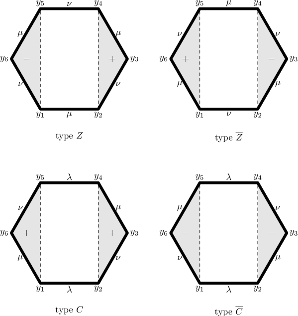
Figure 7. Notation for the bonds of different cell types (top view). Cells of type $C_{\pm}$ and $\overline{C}_{\pm}$ are not illustrated as they are excluded by the reorientation of $H$ of Step 3.

Given the bond $\{y_{i},y_{i+1}\}$ recall that the bond plane containing $y_{i}$, $y_{i+1}$, and $y_{\rm c}$ is oriented via the unit vector $n$ with direction $(y_{i}{-}y_{\rm c})\wedge(y_{i+1}{-}y_{\rm c})$ and define $u=(y_{i+2}{-}y_{i-1}){\cdot}n$. We say that the bond $\{y_{i},y_{i+1}\}$ is of type $\lambda$ if $u=0$, of type $\mu$ if $u>0$, and of type $\nu$ if $u<0$. Note that the bond $\{y_{i},y_{i+1}\}$ is of type $\lambda$ iff the four atoms $\{y_{i-1},y_{i},y_{i+1},y_{i+2}\}$ are coplanar.

This distinction of bond types will turn out useful for discussing mutual cell arrangements. In particular, we say that two cells share a $(\mu,\nu)$ bond if the common bond for such two cells is of type $\mu$ for one cell and of type $\nu$ for the other. Analogously for $(\lambda,\lambda)$ bonds, $(\lambda,\mu)$ bonds etc.

Step 2: Sharing a bond. The aim of this step is to classify the possible mutual arrangements of two cells sharing a bond. This is specified in terms of a corresponding signed incidence angle. By considering the bond angles at the endpoints of the shared bonds which are external to the cells (named external henceforth), we find the admissible values of the signed incidence angles. All possibilities are listed in Table 1 below. We now comment on its entries.

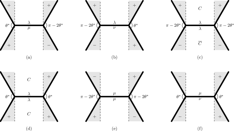
Figure 8. Illustration of the various types of shared bonds for $\gamma=0$. If a triangle with sign $+$ and a triangle with sign $-$ share an atom, the three bonds including such atom are coplanar. Therefore, the external angle is $\pi-2\theta^{*}$. If two triangles with equal sign share an atom, by elementary trigonometry the external angle is $\theta^{*}$, cf. (4.1). These cases correspond to those of Figure 7. In particular, the cases corresponding to cell types $C_{\pm}$ and $\overline{C}_{\pm}$ are not illustrated as they are excluded by the reorientation of $H$ of Step 3.

Type of shared bond	Signed incidence angle	Reference in Figure 8
$(\lambda,\mu)$, $(\lambda,\nu)$	$\not\exists$	(a), (b)
$(\lambda,\lambda)$ ($C$ and $\overline{C}$)	$\pm\gamma^{*}/2$ (not admissible)	(c)
$(\lambda,\lambda)$ (two $C$ cells)	$0,\,-\gamma^{*}$	(d)
$(\lambda,\lambda)$ (two $\overline{C}$ cells)	$0,\,\gamma^{*}$	(d)
$(\mu,\mu)$, $(\nu,\nu)$	$\pm\gamma^{*}/2$	(e)
$(\mu,\nu)$	$0$	(f)

Table 1. Signed incidence angles for various types of shared bonds. Note that the case $(\lambda,\lambda)$ for a $C$ and a $\overline{C}$ cell will be eventually proved to be not admissible in Step 7.

Cases $(\lambda,\mu)$ and $(\lambda,\nu)$: As the two atoms at a $\lambda$ bond and their first neighbors are coplanar, by referring to Figures 8(a) and 8(b) one realizes that the external angles for a $(\lambda,\mu)$ or $(\lambda,\nu)$ bond cannot be both $\theta^{*}$, for any $\gamma$. As a consequence, two cells cannot share a $(\lambda,\mu)$ bond nor a $(\lambda,\nu)$ bond.

Case $(\lambda,\lambda)$: Assume that two cells share a $(\lambda,\lambda)$ bond and let $\gamma$ be the signed incidence angle formed by the corresponding bond planes. As $Z$ and $\overline{Z}$ cells do not have $\lambda$ bonds, see Figure 7, the cells sharing the $(\lambda,\lambda)$ bond are necessarily $C$ or $\overline{C}$. Let a $C$ and a $\overline{C}$ cell share $(\lambda,\lambda)$ bond. By referring to Figure 8(c) one realizes that the incidence angle $\gamma$ at the shared bond cannot be $0$, for this would imply that the external angles are $\pi-2\theta^{*}>\theta^{*}$. Due to symmetry, one finds exactly two symmetric values of the incidence angle ensuring such external angles to be $\theta^{*}$. In particular, we have that $\gamma=\pm\gamma^{*}/2$, where $\gamma^{*}$ is defined in (5.1). The occurrence of a $(\lambda,\lambda)$ bond between a $C$ and a $\overline{C}$ cell will be however proved to be not admissible in Step 7. If both cells are of type $C$, the signed incidence angle $\gamma$ is either $0$, see Figure 8(d), or $-\gamma^{*}$, for these are the only values ensuring that the external angles are $\theta^{*}$. By symmetry, in case both cells are of type $\overline{C}$, the signed incidence angle is either $0$ or $\gamma^{*}$.

Cases $(\mu,\mu)$ and $(\nu,\nu)$: By varying the signed incidence angle $\gamma$, the external angles remain equal and are strictly decreasing with respect to $|\gamma|$. As such external angles are $\pi-2\theta^{*}>\theta^{*}$ for $\gamma=0$, see Figure 8(e) for the case $(\mu,\mu)$, one finds exactly two symmetric values of $\gamma$ making them equal to $\theta^{*}$. By referring to the discussion of the $(\lambda,\lambda)$ bond, one can check that such values are exactly $\pm\gamma^{*}/2$.

Case $(\mu,\nu)$: The external angles are $\theta^{*}$ for $\gamma=0$, see Figure 8(f) and are antimonotone with respect to $|\gamma|$. As such, $\gamma=0$ is the only admissible value for the incidence angle.

Step 3: Reorienting $H$. Given a ground state, we show in this step that one can reorient the reference lattice $H$ in such a way that only the cell types $\{Z,\overline{Z},C,\overline{C}\}$ occur.

Assume that the ground state contains a $C$ cell. By reorienting $H$ one can assume it to be of type $C$ or $\overline{C}$. Letting such cell be indexed by $(s_{0},t_{0})$ we have that cells $(s_{0},t_{0}\pm 1)$ are necessarily either of type $C$ or $\overline{C}$, for they all need to share a $(\lambda,\lambda)$ bond with $(s_{0},t_{0})$. By iterating the argument we have that all cells $(s_{0},t)$, for $t\in\mathbb{Z}$, are either of type $C$ or $\overline{C}$. We now prove that the ground state contains no type $C_{\pm}$ nor $\overline{C}_{\pm}$ cells. Assume indeed that cell $(s_{1},t_{1})$ is of type $C_{-}$ (analogously for $C_{+}$ and $\overline{C}_{\pm}$). Then, the same argument as above entails that all cells $(r,t_{1})$, for $r\in\mathbb{Z}$, are either of type $C_{-}$ or $\overline{C}_{-}$. This, however, brings to a contradiction as cell $(s_{0},t_{1})$ would have to be both of type $C_{-}$ or $\overline{C}_{-}$ and $C$ or $\overline{C}$.

Having fixed the orientation of $H$, all $C$ cells are of type $C$ or $\overline{C}$, so that we just refer to $C$ and $\overline{C}$ cells in the following, omitting the word type. Note that for each $C$ and $\overline{C}$ cell the $\lambda$ bonds are $\{y_{1},y_{2}\}$ and $\{y_{4},y_{5}\}$. If the ground state contains just type $Z$ and $\overline{Z}$ cells, no reorientation of $H$ is actually needed. In all cases, by considering arrangements of cells of a ground state we can always refer to the orientations of Figure 7.

Step 4: Rippled structures, special case. Let us start by considering the special case of two $C$ cells sharing a $(\lambda,\lambda)$ bond with $\gamma=0$. The goal is here to show that two neighboring cells of such $C$ cells must be of the same type (not necessarily $C$) and share a bond with $\gamma=0$. This fact will be used in an induction argument in Step 5.

We can assume with no loss of generality that the joined $C$ cells are $(0,0)$ and $(0,1)$. We proceed by discussing cases.

Case $\tau(1,0)=C$: One has that the shared bond between $(0,0)$ and $(1,0)$ is of type $(\mu,\mu)$. We directly check that $\tau(1,1)\not\in\{Z,\,\overline{Z}\}$ because in this case the cells $(1,0)$ and $(1,1)$ would share a $(\lambda,\mu)$ or a $(\lambda,\nu)$ bond, which is not admissible, see Table 1. The case $\tau(1,1)=\overline{C}$ is also excluded: The $(\mu,\nu)$ bond shared by cells $(0,1)$ and $(1,1)$ requires the corresponding signed incidence angle to be $0$, see Table 1, and the two cells $(1,0)$ and $(1,1)$ would have no shared bond. Indeed, by referring to the notation of Figure 9(a), one has that the three bonds between the cells $(0,0)$, $(1,0)$, the cells $(1,0)$, $(0,1)$, and the cells $(0,1)$, $(1,1)$ are coplanar, the atoms in the darkened regions belong to two parallel planes, whereas atoms $\{y_{1},y_{2},y_{4},y_{5}\}$ of cell $(1,0)$ are not coplanar with those of cell $(1,1)$. As such, the marked bond cannot be shared by cells $(1,0)$ and $(1,1)$.

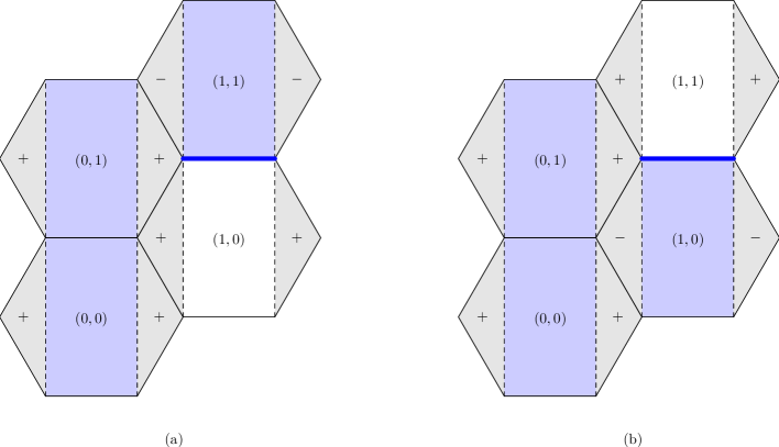
Figure 9. Two nonrealizable configurations.

The only possibility left is $\tau(1,1)=C$, which can indeed be realized by letting the signed incidence angle along the shared bond between cells $(1,0)$ and $(1,1)$ be $0$.

Case $\tau(1,0)=\overline{C}$: One can again check that $\tau(1,1)\not\in\{Z,\,\overline{Z}\}$ because in this case the cells $(1,0)$ and $(1,1)$ would share a $(\lambda,\mu)$ or a $(\lambda,\nu)$ bond, which is not admissible. Moreover, the case $\tau(1,1)=C$ can be excluded arguing similarly as above: By referring to Figure 9(b) one has that the three bonds between the cells $(0,0)$, $(1,0)$, the cells $(1,0)$, $(0,1)$, and the cells $(0,1)$, $(1,1)$ are coplanar, the atoms in the darkened regions belong to two parallel planes, whereas atoms $\{y_{1},y_{2},y_{4},y_{5}\}$ of cell $(1,0)$ are not coplanar with those of cell $(1,1)$. In particular, the marked bond cannot be shared by cells $(1,0)$ and $(1,1)$. We are left with the possibility of having $\tau(1,1)=\overline{C}$, which can indeed be realized by letting the signed incidence angle along the shared bond between cells $(1,0)$ and $(1,1)$ be $0$.

Case $\tau(1,0)=Z$: One can argue exactly as in the case of $\tau(1,0)=\overline{C}$ and find that $\tau(1,1)=Z$ as well, with a signed incidence angle along the shared bond between $(1,0)$ and $(1,1)$ being $0$. Indeed, one can still refer to Figure 9(b) by forgetting the two right-most atoms.

Case $\tau(1,0)=\overline{Z}$: One can argue exactly as in the case of $\tau(1,0)=C$ and find that $\tau(1,1)=\overline{Z}$ as well, with a signed incidence angle along the shared bond between $(1,0)$ and $(1,1)$ being $0$. This case corresponds to Figure 9(a) upon forgetting the two right-most atoms.

In conclusion, within this step we have proved the following

$$\tau(0,0)=\tau(0,1)=C\ \ \text{and}\ \ \gamma=0\ \ \text{along the shared $(\lambda,\lambda)$ bond}$$

$$\Longrightarrow\quad\tau(1,0)=\tau(1,1)\ \ \text{and}\ \ \gamma=0\ \ \text{along the shared bond}.$$ (5.3)

Step 5: Rippled structures, general case. The argument of Step 4 is purely based on bond types. As such, it can be verbatim extended to case $\tau(0,0)=\tau(0,1)\in\{Z,\overline{Z},\overline{C}\}$ as long as $\gamma=0$ along their shared bond. In addition, conclusion (5.3) can be extended by symmetry to cell $(1,-1)$ and cells $(-1,0)$, $(-1,1)$, and $(-1,2)$ as well. We hence have the following

$$\tau(0,0)=\tau(0,1)\ \ \text{and}\ \ \gamma=0\ \ \text{along the shared bond}$$

$$\Longrightarrow\quad\tau(-1,0)=\tau(-1,1)=\tau(-1,2)\ \ \ \text{and}\ \ \ \tau(1,-1)=\tau(1,0)=\tau(1,1)\ \$$

$$\text{and}\ \ \gamma=0\ \ \text{along the shared bonds}.$$ (5.4)

We can now use (5.4) iteratively and prove that if $\tau(0,0)=\tau(0,1)$ with $\gamma=0$ along the shared bond. then $\tau(s,\cdot)$ is constant for all $s\in\mathbb{Z}$ and $\widehat{\gamma}(s,t)=0$ for all $(s,t)\in\mathbb{Z}^{2}$. Note that all cell types $\{Z,\overline{Z},C,\overline{C}\}$ are admissible for $\tau(s,\cdot)$.

This proves the Theorem in case $\tau(0,0)=\tau(0,1)$ with $\gamma=0$ along the shared bond.

Step 6: Zigzag roll-ups. Let us now consider the case of two $C$ cells sharing a $(\lambda,\lambda)$ bond with $\gamma=-\gamma^{*}$. The goal is here to show that $\tau\equiv C$ and $\widehat{\gamma}\equiv-\gamma^{*}$.

As in Step 4, assume with no loss of generality that the $C$ cells are $(0,0)$ and $(0,1)$, namely $\tau(0,0)=\tau(0,1)=C$. We aim at proving that $\tau(1,0)=\tau(1,1)=C$ as well, which would imply that the signed incidence angle of the shared $(\lambda,\lambda)$ bond between $(1,0)$ and $(1,1)$ is again $-\gamma^{*}$.

Case $\tau(1,0)\in\{\overline{C},Z\}$ (not admissible): If this was the case, cell $(1,0)$ would share a $(\mu,\nu)$ bond with cell $(0,0)$. According to Table 1, the two corresponding signed incidence angles for $\overline{C}$ and $Z$, respectively, would be $0$. This in particular entails that the atoms $\{y_{2},y_{3},y_{4}\}$ of cell $(0,0)$ and $\{y_{1},y_{5},y_{6}\}$ of cell $(1,0)$ have to be coplanar. At the same time, cell $(1,0)$ would share a $(\mu,\nu)$ bond with cell $(0,1)$ and the atoms $\{y_{2},y_{3},y_{4}\}$ of cell $(0,1)$ and $\{y_{1},y_{5},y_{6}\}$ of cell $(1,0)$ would have to be coplanar. This is however impossible as the atoms $\{y_{2},y_{3},y_{4}\}$ in the two cells $(0,0)$ and $(0,1)$ are not coplanar, due to the condition $\gamma=-\gamma^{*}$ along the shared bond between cells $(0,0)$ and $(0,1)$.

Case $\tau(1,0)=\overline{Z}$ (not admissible): Assume that this was the case and consider cell $(1,1)$. This cannot be of type $C$ nor $\overline{C}$, for in this case cell $(1,1)$ would share a $(\lambda,\mu)$ bond (not admissible by Table 1) with cell $(1,0)$. On the other hand, cell $(1,1)$ cannot be of type $\overline{Z}$ as in this case it would share a $(\mu,\nu)$ bond with cell $(1,0)$ and the corresponding signed incidence angle $0$. We could then apply Step 5 in order to find that the signed incidence angle between cell $(0,0)$ and $(0,1)$ would have to be $0$ as well, which is a contradiction. The last possibility is that cell $(1,1)$ is of type $Z$. In this case, cell $(1,1)$ and cell $(0,1)$ share a $(\mu,\nu)$ bond and thus the signed incidence angle along the shared bond is $0$, see Table 1. Similarly to the case of Figure 9(a), cell $(1,1)$ would not share a bond with cell $(1,0)$.

Case $\tau(1,0)=C$: We have hence proved that, given $\tau(0,0)=\tau(0,1)=C$ with signed incidence angle $-\gamma^{*}$ along the shared $(\lambda,\lambda)$ bond, the only possible type of cell $(1,0)$ is $C$. Cells $(1,1)$ and $(1,-1)$ need then to be of type $C$ or $\overline{C}$ as well, for they have to share a $\lambda$ bond with cell $(1,0)$. One can however exclude that they are of type $\overline{C}$ since in this case the signed incidence angle to cell $(0,1)$ or cell $(0,0)$, respectively, would be $0$ and they would not share a bond with cell $(1,0)$. We again refer to Figure 9(a) for a similar argument.

In conclusion, if $\tau(0,0)=\tau(0,1)=C$ with signed incidence angle $-\gamma^{*}$ along the shared bond, one has that $\tau(1,1)=\tau(1,0)=\tau(1,-1)=C$. This can indeed be realized by letting the signed incidence angle along the shared bond between cells $(1,1)$, $(1,0)$ and $(1,0)$, $(1,-1)$ be $-\gamma^{*}$. By symmetry, the same holds for cells $(-1,2)$, $(-1,1)$, and $(-1,0)$ as well. It is now easy to proceed by induction in order to prove that indeed $\tau(s,t)=C$ and $\widehat{\gamma}(s,t)=-\gamma^{*}$ for all $(s,t)\in\mathbb{Z}^{2}$.

An analogous conclusion obviously holds in case $\tau(0,0)=\tau(0,1)=\overline{C}$ with signed incidence angle $\gamma^{*}$. In this case, $\tau(s,t)=\overline{C}$ and $\widehat{\gamma}(s,t)=\gamma^{*}$ for all $(s,t)\in\mathbb{Z}^{2}$. This proves the Theorem in case $\tau(0,0)=\tau(0,1)\in\{C,\,\overline{C}\}$ with $\gamma=\mp\gamma^{*}$ along the shared bond.

Step 7: Nonadmissible configurations containing $C$ and $\overline{C}$ cells. In order to conclude the proof of the Theorem, one needs to check that no other configurations of optimal cells are admissible but those already considered in Steps 5 and 6. This is done here and in Step 8.

If a ground state contains a $C$ or a $\overline{C}$ cell, it contains infinitely many as these are the only ones that can share $\lambda$ bonds. Assume that cell $(0,0)$ is of type $C$. Then, all cells $(0,t)$ are either $C$ or $\overline{C}$, see Step 3. If two adjacent cells $(0,t)$ are of the same type, one has that $t\mapsto\tau(0,t)$ is constant, due to Step 4. One is then left with the possibility that $\tau(0,t)=C$ for $t$ even and $\tau(0,t)=\overline{C}$ for $t$ odd. The rest of the step is aimed at proving that such an alternation of types is not admissible.

Let us start by checking that a configuration with

$$\tau(s,t)=C\ \ \text{if $s+t$ is even},\quad\tau(s,t)=\overline{C}\ \ \text{if $s+t$ is odd, for $s=0,1$,}$$ (5.5)

is not admissible. Indeed, in this case the four coplanar atoms of cell $(0,0)$ and those of cell $(1,0)$ belong to parallel planes and atoms $\{y_{2},y_{3},y_{4}\}$ of cell $(0,0)$ and $\{y_{1},y_{5},y_{6}\}$ of cell $(1,0)$ are coplanar, see the darkened region in Figure 10. At the same time, the four coplanar atoms of cell $(0,1)$ and those of cell $(1,1)$ belong to parallel planes and atoms $\{y_{2},y_{3},y_{4}\}$ of cell $(0,1)$ and $\{y_{1},y_{5},y_{6}\}$ of cell $(1,1)$ are coplanar. This, however, excludes that cells $(0,0)$, $(1,0)$ and cells $(0,1)$, $(1,1)$ simultaneously share the three marked bonds in Figure 10 and configuration (5.5) is not admissible. By symmetry, the configuration

$$\tau(s,t)=C\ \ \text{if $t$ is even},\quad\tau(s,t)=\overline{C}\ \ \text{if $t$ is odd, for $s=0,1$,}$$ (5.6)

is not admissible as well.

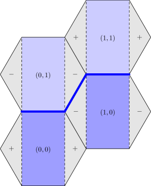
Figure 10. Configuration (5.5) is not admissible.

Assume now that $\tau(0,t)=C$ for $t$ even and $\tau(0,t)=\overline{C}$ for $t$ odd and $\tau(1,t)\in\{Z,\overline{Z}\}$. We can assume that neighboring cells $(1,t)$ are of different types since otherwise one would have a signed incidence angle $0$ along a shared bond (see Figure 7 and Table 1) and we would be in the situation of Step 5, see (5.4). If $\tau(1,0)=Z$, we can argue exactly in the case of (5.5) (by forgetting the two right-most atoms in Figure 10) and find that the configuration is not admissible. Analogously, the case $\tau(1,0)=\overline{Z}$ can be excluded by arguing as for (5.6).

Step 8: Conclusion of the proof. Let us now check that the previous steps exhaust all possible cases and that the statement holds.

If the ground state contains a $C$ cell (analogously, a $\overline{C}$ cell), then we are in the situations of Steps 5 or 6 as all other possibilities are excluded by Step 7 and Table 1. In case the ground state contains just $Z$ or $\overline{Z}$, two cells of the same type have to share a bond and this has to be of type $(\mu,\nu)$ (recall the orientations from Figure 7). The corresponding incidence angle is $0$ and, after possible reorientation of $H$, we are in the situation of (5.4) (Step 5). ∎

References

- [1] D. W. Brenner. Empirical potential for hydrocarbons for use in stimulating the chemical vapor deposition of diamond films, Phys. Rev. B, 42 (1990), 9458–9471.
- [2] J. Clayden, N. Greeves, S. G. Warren. Organic chemistry, Oxford University Press, 2012.
- [3] C. Davini, A. Favata, R. Paroni. The Gaussian stiffness of graphene deduced from a continuum model based on molecular dynamics potentials, J. Mech. Phys. Solids, 104 (2017), 96–114.
- [4] E. Davoli, P. Piovano, U. Stefanelli. Wulff shape emergence in graphene, Math. Models Methods Appl. Sci. 26 (2016), 2277–2310.
- [5] S. Deng, V. Berry. Wrinkled, rippled and crumpled graphene: an overview of formation mechanism, electronic properties, and applications, Mater. Today, 19 (4)(2016), 197–212.
- [6] W. E, D. Li. On the crystallization of 2D hexagonal lattices, Comm. Math. Phys. 286 (2009), 3:1099–1140.
- [7] B. Farmer, S. Esedoḡlu, P. Smereka. Crystallization for a Brenner-like potential, Comm. Math. Phys. 349 (2017), 1029–1061.
- [8] C. P. Herrero, R. Ramirez. Quantum effects in graphene monolayers: Path-integral simulations. J. Chem. Phys. 145 (2016), 224701.
- [9] A. Fasolino, J. H. Los, M. I. Katsnelson. Intrinsic ripples in graphene, Nature Materials, 6 (2007), 858–861.
- [10] A. C. Ferrari et al. Science and technology roadmap for graphene, related two-dimensional crystals, and hybrid systems, Nanoscale, 7 (2015), 4587–5062.
- [11] M. Friedrich, E. Mainini, P. Piovano, U. Stefanelli. Characterization of optimal carbon nanotubes under stretching and validation of the Cauchy-Born rule. Submitted, 2017. Preprint at arXiv:1706.01494.
- [12] M. Friedrich, P. Piovano, U. Stefanelli. The geometry of , SIAM J. Appl. Math. 76 (2016), 2009–2029.
- [13] M. Friedrich, U. Stefanelli. Periodic ripples in graphene: a variational approach. Submitted, 2018. Preprint at arXiv:1802.05053.
- [14] P. Lambin. Elastic properties and stability of physisorbed graphene, Appl. Sci. 4 (2014), 282–304.
- [15] L. D. Landau, E. M. Lifshitz. Statistical Physics, Pergamon, Oxford, 1980.
- [16] G. Lazzaroni, U. Stefanelli. Chain-like minimizers in three dimensions. Submitted, 2017. Preprint available at http://cvgmt.sns.it/paper/3418/
- [17] E. Mainini, H. Murakawa, P. Piovano, U. Stefanelli. Carbon-nanotube geometries: analytical and numerical results, Discrete Contin. Dyn. Syst. Ser. S, 10 (2017), 141–160.
- [18] E. Mainini, H. Murakawa, P. Piovano, U. Stefanelli. Carbon-nanotube geometries as optimal configurations. Multiscale Model. Simul. 15 (2017), 1448–1471.
- [19] E. Mainini, U. Stefanelli. Crystallization in carbon nanostructures, Comm. Math. Phys. 328 (2014), 2:545–571.
- [20] N. D. Mermin. Crystalline order in two dimensions, Phys. Rev. 176 (1968), 250–254.
- [21] N. D. Mermin, H. Wagner. Absence of ferromagnetism or antiferromagnetism in one- or two-dimensional isotropic Heisenberg models, Phys. Rev. Lett. 17 (1966), 1133–1136.
- [22] J. C. Meyer, A. K. Geim, M. I. Katsnelson, K. S. Novoselov, T. J. Booth, S. Roth. The structure of suspended graphene sheets, Nature 446 (2007), 60–63.
- [23] U. Stefanelli. Stable carbon configurations, Boll. Unione Mat. Ital (9), 10 (2017), 335–354.
- [24] F. H. Stillinger, T. A. Weber. Computer simulation of local order in condensed phases of silicon, Phys. Rev. B, 8 (1985), 5262–5271.
- [25] J. Tersoff. New empirical approach for the structure and energy of covalent systems, Phys. Rev. B, 37 (1988), 6991–7000.
- [26] F. Theil. A proof of crystallization in two dimensions, Comm. Math. Phys. 262 (2006), 1:209–236.