Parameter estimation for discretely-observed linear birth-and-death processes

Abstract

Birth-and-death processes are widely used to model the development of biological populations. Although they are relatively simple models, their parameters can be challenging to estimate, because the likelihood can become numerically unstable when data arise from the most common sampling schemes, such as annual population censuses. Simple estimators may be based on an embedded Galton-Watson process, but this presupposes that the observation times are equi-spaced. We estimate the birth, death, and growth rates of a linear birth-and-death process whose population size is periodically observed via an embedded Galton–Watson process, and by maximizing a saddlepoint approximation to the likelihood. We show that a Gaussian approximation to the saddlepoint-based likelihood connects the two approaches, we establish consistency and asymptotic normality of quasi-likelihood estimators, compare our estimators on some numerical examples, and apply our results to census data for two endangered bird populations and the H1N1 influenza pandemic.

Keywords: Galton–Watson process; Gaussian approximation; likelihood inference; linear birth-and-death process; saddlepoint approximation.

1 Introduction

Linear birth-and-death processes are among the simplest and most widely-used continuous-time Markovian population models, with many applications in biology, genetics, and ecology [17, 25]. Most estimation methods rely on continuous observation of the population, which allows maximum likelihood estimation of the birth and death rates $\lambda$ and $\mu$ [18]. Continuous measurement is rare in practice, however, and often observations are available only at discrete time points. For example, data in population biology typically arise from annual animal censuses. Likelihood-based estimation is then difficult owing to the cumbersome and numerically unstable form of the probability mass function of the population size.

Several authors have proposed approaches to address this instability, and more generally to estimate the parameters of discretely-observed general birth-and-death processes, for which an analytic expression for the population size distribution may be unavailable. Chen and Hyrien [3] propose quasi- and pseudo-likelihood estimators, but their empirical analysis suggests that these are inferior to the maximum likelihood estimator (MLE). Crawford and Suchard [5] and Crawford et al. [4] use continued fractions to obtain expressions for the Laplace transform of the population size distribution. They approach the computation of the likelihood as a missing data problem, and maximize it using an expectation-maximization (EM) algorithm. This is also used in Xu et al. [30], who propose a multitype branching process approximation to birth-death-shift processes, but their method has numerical limitations in settings with very large populations. Ross et al. [27] estimate discretely-observed density-dependent Markov population processes using an approximation based on a deterministic model combined with a Gaussian diffusion.

After sketching the properties of linear birth-and-death processes in Section 2, we propose two alternative efficient ways to estimate their parameters from discrete-time data. The first approach, developed in Section 3, assumes equal inter-observation times, and uses the Galton–Watson process embedded at the successive observation times. We derive asymptotic properties of the resulting estimators for $\lambda$, $\mu$, and for the growth rate $\omega=\lambda-\mu$. Keiding [18] used a similar approach, but under the additional assumption that one observes the number of individuals with no offspring at each generation in the embedded process. His estimators correspond to MLEs, while in our case only the estimator of $\omega$ is the MLE from the discretely-observed process.

Our second approach, detailed in Section 4, needs no constraint on the inter-observation times, and is based on a saddlepoint approximation to the population size distribution, leading to saddlepoint MLEs. Saddlepoint methods provide accurate approximations in many applications: Daniels [7] applies them to general birth processes; Aı and Yu [1] use them to construct closed-form approximations to the transition densities of continuous-time Markov processes; and Pedeli et al. [26] use them to estimate high-order integer-valued autoregressive processes, and show the high accuracy of the resulting approximate MLEs. We highlight the gain in computational efficiency when using the saddlepoint technique to approximate the population size distribution compared to evaluating its analytical form, discuss the approximation error, show that the estimators obtained with the embedded Galton–Watson approach correspond to MLEs based on a Gaussian simplification of the saddlepoint approximation, and establish consistency and asymptotic normality of these estimators for unequal observation intervals.

Simulations in Section 5 indicate that the relative error between the saddlepoint and true MLEs quickly becomes negligible as the observed population size increases. The saddlepoint MLEs always have lower mean square error than the Galton–Watson estimators, but they become comparable if one increases the number of discrete observations of a non-extinct population, or its size at the first observation time. Section 6 illustrates our ideas with real censuses of two endangered bird populations and the H1N1 influenza pandemic. All lengthy proofs may be found in Appendix A.

2 Discretely observed linear birth-and-death processes

A linear birth-and-death process (LBDP) with birth rate $\lambda$ and death rate $\mu$ is a continuous-time Markovian branching process in which an individual lifetime is exponentially distributed with parameter $\mu$ and reproduction occurs according to a Poisson process with parameter $\lambda$. The population size increases from $k$ to $k+1$ at rate $k\lambda$, or decreases to $k-1$ at rate $k\mu$. The population growth rate, $\omega:=\lambda-\mu$, is also called the Malthusian parameter.

The conditional probability mass function of the population size $Z(t)$ at time $t$, given $Z(0)=a$, is denoted by ${p}_{k}(t;a):=\mathsf{P}\{Z(t)=k\,|\,Z(0)=a\}$ for $a,k\in\mathbb{Z}^{+}.$ The corresponding probability generating function (PGF) is $f(s,t;a):=\sum_{k\geq 0}p_{k}(t;a)s^{k}=f(s,t)^{a},$ where $f(s,t):=f(s,t;1)$ satisfies the backward Kolmogorov equation

$$\frac{\partial f(s,t)}{\partial t}=\mu-(\lambda+\mu)f(s,t)+\lambda^{2}f(s,t)^{2},\qquad f(s,0)=s,$$

and this has explicit solution

$$f(s,t)=\left\{\begin{array}[]{ll}1+\dfrac{(\lambda-\mu)(s-1)}{(\lambda s-\mu)\,\exp{(\mu-\lambda)t}-\lambda(s-1)},&\lambda\neq\mu,\\[10.00002pt] 1+\dfrac{(s-1)}{1-\lambda t(s-1)},&\lambda=\mu.\end{array}\right.$$ (2.1)

The distribution of $Z(t)$ conditional on $Z(0)=1$ corresponds to a modified geometric distribution, $p_{k}(t;1)=\alpha(t)\,\mathds{1}_{\{k=0\}}+\{1-\alpha(t)\}\{1-\beta(t)\}\beta(t)^{k-1}\,\mathds{1}_{\{k>0\}}$, where $\mathds{1}_{\{\cdot\}}$ denotes the indicator function, with

$$\alpha(t)=\left\{\begin{array}[]{ll}\dfrac{\mu\{\exp{\omega t}-1\}}{\lambda\exp{\omega t}-\mu},&\lambda\neq\mu,\\[10.00002pt] \dfrac{\lambda t}{1+\lambda t},&\lambda=\mu,\end{array}\right.\qquad\beta(t)=\left\{\begin{array}[]{ll}\dfrac{\lambda}{\mu}\alpha(t),&\lambda\neq\mu,\\[10.00002pt] \alpha(t),&\lambda=\mu.\end{array}\right.$$

Conditionally on $Z(0)=a$ and by independence of the individuals, $p_{0}(t;a)=\alpha(t)^{a}$, and for $k\geq 1$, by conditioning on the number of ancestors whose descendence becomes extinct by time $t$, we obtain [15, p. 47, with some typos corrected here]:

$$p_{k}(t;a)=\sum_{j=\max(0,a-k)}^{a-1}\binom{a}{j}\binom{k-1}{a-j-1}\alpha(t)^{j}\,[\{1-\alpha(t)\}\{1-\beta(t)\}]^{a-j}\,\beta(t)^{k-a+j}.$$ (2.2)

The conditional mean and variance of the population size at time $t$ are respectively

$$m(t;a) =\mathsf{E}\{Z(t)\,|\,Z(0)=a\}=a\,\exp(\omega t),$$ (2.3)

$$\sigma^{2}(t;a) =\mathsf{Var}\{Z(t)\,|\,Z(0)=a\}=\left\{\begin{array}[]{ll}a\,\frac{\lambda+\mu}{\omega}\,\exp(\omega t)\{\exp(\omega t)-1\},&\lambda\neq\mu,\\[10.00002pt] a\,2\lambda t,&\lambda=\mu.\end{array}\right.$$ (2.6)

When $a=1$, we write $m(t):=m(t;1)$ and $\sigma^{2}(t):=\sigma^{2}(t;1)$.

Suppose that $M$ independent trajectories of an LBDP are discretely observed $N+1$ times, with $M,N\geq 1$, and for $i=1,\ldots,M$ and $j=0,\ldots,N$ let $t_{i,j}$ and $k_{i,j}$ denote the time and population size corresponding to the $(j+1)$st observation of the $i$th trajectory. The log-likelihood based on observations $\bm{t}:=\{t_{i,j}\}$ and $\bm{k}:=\{k_{i,j}\}$ is

$$\ell(\lambda,\mu;\bm{t},\bm{k}) = \sum_{i=1}^{M}\log\mathsf{P}\{Z(t_{i,1})=k_{i,1},\ldots,Z(t_{i,N})=k_{i,N}\,|\,Z(0)=k_{i,0}\}$$ (2.7)

$$= \sum_{i=1}^{M}\sum_{j=1}^{N}\log\mathsf{P}\{Z(t_{i,j}-t_{i,j-1})=k_{i,j}\,|\,Z(0)=k_{i,j-1}\},$$ (2.8)

where (2.8) follows from the Markov property. Computing the MLEs of $\lambda$ and $\mu$ therefore requires the efficient calculation of ${p}_{k}(t;a)$ for any $a,k\in\mathbb{Z}^{+}$ and $t\in\mathbb{R}^{+}$. Despite the explicit form (2.2) of these probabilities, the binomial coefficients for large values of $k$ or $a$ are very large, leading to numerical difficulties and making the maximization of (2.8) cumbersome, if not impossible. These issues, mentioned earlier in the literature (for example in [8, 3]), hamper the use of likelihood estimation of $\lambda$ and $\mu$ from discrete observations. In the next two sections we propose methods to circumvent them.

3 Embedded Galton–Watson process approach

If the inter-observation times all equal $\Delta t$, the discretely-observed LBDP corresponds to a Galton–Watson (GW) process with progeny generating function $P(s):=f(s,\Delta t)$ and offspring mean and variance $m:=m(\Delta t;1)$ and $\sigma^{2}:=\sigma^{2}(\Delta t;1)$, where $m(t;a)$ and $\sigma^{2}(t;a)$ are defined in (2.3) and (2.6) [16, p. 101]. The birth and death rates may be expressed as

$$\lambda=\frac{\log m}{2\Delta t}\left\{\frac{\sigma^{2}}{m(m-1)}+1\right\},\quad\mu=\frac{\log m}{2\Delta t}\left\{\frac{\sigma^{2}}{m(m-1)}-1\right\},$$ (3.1)

in the non-critical case, and

$$\lambda=\mu=\frac{\sigma^{2}}{2t}$$ (3.2)

in the critical case, which allows simple estimation of them using the offspring mean and variance of the embedded GW process. We call this the GW approach. We start by sketching the properties of these estimators based on a single trajectory, $M=1$.

Based on the observation of the initial population size $Z_{0}:=Z(0)$ and the successive population sizes $Z_{1}:=Z(\Delta t),\ldots,Z_{N}:=Z(N\Delta t)$ in the $N$ subsequent generations of the embedded GW process, the natural estimators of $m$ and $\sigma^{2}$ are

$$\hat{m}_{Z_{0},N}=\frac{\sum_{n=1}^{N}Z_{n}}{\sum_{n=0}^{N-1}Z_{n}},\quad\widehat{\sigma^{2}}_{Z_{0},N}=\frac{1}{N}\,\sum_{n=1}^{N}Z_{n-1}\left(\frac{Z_{n}}{Z_{n-1}}-\hat{m}_{Z_{0},N}\right)^{2}.$$ (3.3)

In particular, $\hat{m}_{Z_{0},N}$ corresponds to a method of moments, conditional least squares and MLE of $m$ [15, Chapter 2]. There is a possibility of division by zero in $\widehat{\sigma^{2}}_{Z_{0},N}$, but if $Z_{n-1}=0$, then $Z_{n}=0$ as well, and we may set $Z_{n}/Z_{n-1}:=1$ so that the corresponding term vanishes. This only happens if the process becomes extinct.

Asymptotic properties of $\hat{m}_{Z_{0},N}$ and $\widehat{\sigma^{2}}_{Z_{0},N}$ have been studied extensively. As $N\to\infty$, and conditionally on the eventual explosion of the process, $\{Z_{N}\to\infty\}$, both estimators are consistent and asymptotically normal [15]:

$$\sqrt{\frac{\sum_{n=1}^{N}Z_{n-1}}{\sigma^{2}}}\big{(}\hat{m}_{Z_{0},N}-m\big{)} \xrightarrow[]{d} \mathcal{N}(0,1),$$ (3.4)

$$\sqrt{\frac{N}{2\sigma^{4}}}\big{(}\widehat{\sigma^{2}}_{Z_{0},N}-\sigma^{2}\big{)} \xrightarrow[]{d} \mathcal{N}(0,1),$$ (3.5)

where $\xrightarrow[]{d}$ denotes convergence in distribution. These results hold for any fixed value of $Z_{0}$ but only for supercritical processes ($m>1$), since otherwise eventual explosion has probability zero.

If both $Z_{0}\to\infty$ and $N\to\infty$, and conditionally on $\{Z_{N}\to\infty\}$, it can be shown that the estimators are consistent and jointly asymptotically normal [11]:

$$\left(\begin{matrix}\sqrt{\frac{Z_{0}\,(m^{N}-1)}{\sigma^{2}\,(m-1)}}\,(\hat{m}_{Z_{0},N}-m)\\ \sqrt{\frac{N}{2\sigma^{4}}}(\widehat{\sigma^{2}}_{Z_{0},N}-\sigma^{2})\\ \end{matrix}\right)\xrightarrow[]{d}\mathcal{N}\left(\mathbf{0},\mathbf{I}\right),$$ (3.6)

where $\mathcal{N}(\mathbf{0},\mathbf{I})$ is the bivariate normal distribution with independent standard normal marginals.

If $Z_{0}\to\infty$ but $N$ is fixed, results on consistency and asymptotic normality are available for $\hat{m}_{Z_{0},N}$ but not for $\widehat{\sigma^{2}}_{Z_{0},N}$. For critical and subcritical processes, for which $m=1$ and $m<1$ respectively, results on consistency and marginal asymptotic normality of $\hat{m}_{Z_{0},N}$ and $\widehat{\sigma^{2}}_{Z_{0},N}$ are also available if both $Z_{0}\to\infty$ and $N\to\infty$, under additional assumptions on their relative speed of convergence [15, 10]. We shall not explore these cases further here.

On inserting the estimators $\hat{m}_{Z_{0},N}$ and $\widehat{\sigma^{2}}_{Z_{0},N}$ from (3.3) into (3.1), we obtain estimators

$$\hat{\lambda}_{Z_{0},N} = \frac{\log\hat{m}_{Z_{0},N}}{2\Delta t}\left\{\frac{\widehat{\sigma^{2}}_{Z_{0},N}}{\hat{m}_{Z_{0},N}(\hat{m}_{Z_{0},N}-1)}+1\right\},$$ (3.7)

$$\hat{\mu}_{Z_{0},N} = \frac{\log\hat{m}_{Z_{0},N}}{2\Delta t}\left\{\frac{\widehat{\sigma^{2}}_{Z_{0},N}}{\hat{m}_{Z_{0},N}(\hat{m}_{Z_{0},N}-1)}-1\right\},$$ (3.8)

whose properties can be derived from those of $\hat{m}_{Z_{0},N}$ and $\widehat{\sigma^{2}}_{Z_{0},N}$, as shown in the next theorem, whose proof is in Appendix A.

Theorem 1.

Suppose that $m>1$. Then $\hat{\lambda}_{Z_{0},N}$ and $\hat{\mu}_{Z_{0},N}$ are consistent on $\{Z_{N}\to\infty\}$ as $N\to\infty$, and also as both $N\to\infty$ and $Z_{0}\to\infty$.

Moreover,

$$\sqrt{N}\,\left(\begin{matrix}\hat{\lambda}_{Z_{0},N}-\lambda\\ \hat{\mu}_{Z_{0},N}-\mu\end{matrix}\right)\xrightarrow[]{d}\mathcal{N}\left\{\left(\begin{matrix}0\\ 0\\ \end{matrix}\right),\frac{(\log m)^{2}\sigma^{4}}{2(\Delta t)^{2}m^{2}(m-1)^{2}}\times\left(\begin{matrix}1&1\\ 1&1\\ \end{matrix}\right)\right\}$$

conditionally on $\{Z_{N}\to\infty\}$ as $N\to\infty$, and also as both $N\to\infty$ and $Z_{0}\to\infty$.

By Theorem 1, the difference $\sqrt{N}\,\big{\{}(\hat{\lambda}_{Z_{0},N}-\lambda)-(\hat{\mu}_{Z_{0},N}-\mu)\big{\}}$ vanishes in probability conditional on $\{Z_{N}\to\infty\}$ as $N\to\infty$ and also as both $N\to\infty$ and $Z_{0}\to\infty$. Thus, the estimator $\hat{\omega}_{Z_{0},N}=\hat{\lambda}_{Z_{0},N}-\hat{\mu}_{Z_{0},N}$ of the Malthusian parameter $\omega$ satisfies $\sqrt{N}(\hat{\omega}_{Z_{0},N}-\omega)\xrightarrow[]{p}0$ conditionally on $\{Z_{N}\to\infty\}$ as $N\to\infty$, and also as both $N\to\infty$ and $Z_{0}\to\infty$, where $\xrightarrow[]{p}$ denotes the convergence in probability. This is no surprise, as $\hat{\omega}_{Z_{0},N}=\log(\hat{m}_{Z_{0},N})/\Delta t$ is a function of $\hat{m}_{Z_{0},N}$ only. Asymptotic normality for $\hat{\omega}_{Z_{0},N}$ is therefore achieved at a higher rate of convergence than for $\hat{\lambda}_{Z_{0},N}$ and $\hat{\mu}_{Z_{0},N}$.

Theorem 2.

Suppose that $m>1$. Then $\hat{\omega}_{Z_{0},N}$ is consistent on $\{Z_{N}\to\infty\}$ as $N\to\infty$ and also as both $N\to\infty$ and $Z_{0}\to\infty$.

Moreover,

$$\sqrt{\sum_{n=1}^{N}Z_{n-1}}\times\big{(}\hat{\omega}_{Z_{0},N}-\omega\big{)}\xrightarrow[]{d}\mathcal{N}\left\{0,\frac{\sigma^{2}}{m^{2}(\Delta t)^{2}}\right\}$$

conditionally on $\{Z_{N}\to\infty\}$ as $N\to\infty$, and

$$\sqrt{Z_{0}\,(m^{N}-1)}\times\big{(}\hat{\omega}_{Z_{0},N}-\omega\big{)}\xrightarrow[]{d}\mathcal{N}\left\{0,\frac{\sigma^{2}(m-1)}{m^{2}(\Delta t)^{2}}\right\}$$

conditionally on $\{Z_{N}\to\infty\}$ as $N\to\infty$ and $Z_{0}\to\infty$.

Proof.

Consistency of $\hat{\omega}_{Z_{0},N}$ follows from consistency of $\hat{m}_{Z_{0},N}$; asymptotic normality of $\hat{\omega}_{Z_{0},N}$ follows from asymptotic normality of $\hat{m}_{Z_{0},N}$ and application of the delta method. ∎

Suppose now that we observe multiple independent trajectories of the LBDP, i.e., $M>1$, and that the inter-observation times are constant and equal $\Delta t$ for all trajectories, so that we observe $M$ independent trajectories of the embedded GW process. Let $Z_{i,n}:=Z_{i}(n\Delta t)$ be the $n^{\text{th}}$ observation of the $i^{\text{th}}$ trajectory for $i\in\{1,\ldots,M\}$ and $n\in\{0,\ldots,N\}$. The estimators of the offspring mean and variance of the GW process are then

$$\hat{m}_{M,N}=\frac{\sum_{i=1}^{M}\sum_{j=1}^{N}Z_{i,j}}{\sum_{i=1}^{M}\sum_{j=-1}^{N}Z_{i,j-1}},\quad\widehat{\sigma^{2}}_{M,N}=\frac{1}{MN}\,\sum_{i=1}^{M}\sum_{j=1}^{N}Z_{i,j-1}\left(\frac{Z_{i,j}}{Z_{i,j-1}}-\hat{m}_{M,N}\right)^{2}.$$ (3.9)

Again, we set $0/0:=1$ if any of the trajectories becomes extinct. These estimators appear not to have been analysed previously. We derive them in Section 5, and establish the consistency and asymptotic normality of the corresponding estimators for $\lambda$ and $\mu$.

4 Saddlepoint approximation

Saddlepoint approximation offers a very accurate way to approximate probability distributions [6, 2]. It is particularly useful when these distributions are intractable, or when their numerical evaluation is unstable, as in our context.

The conditional cumulant generating function (CGF) of the population size $Z(t)$ at time $t$, given $Z(0)=a$, is defined as $K(x,t;a):=\log M(x,t;a),$ where $M(x,t;a):=f(\exp(\omega t),t;a)$ is the conditional moment generating function. Its maximal convergence set in a neighbourhood of $0$ is $\mathcal{S}(t)=(-\infty,\log R(t))$, where

$$R(t)=\left\{\begin{array}[]{ll}1+\dfrac{\omega}{\lambda\{\exp(\omega t)-1\}},&\lambda\neq\mu,\\[10.00002pt] 1+\dfrac{1}{\lambda t},&\lambda=\mu.\end{array}\right.$$

When $k=0$ we have $p_{0}(t;a)=\alpha(t)^{a}$ and no approximation is needed. For $k=1,2,\ldots$, the (first-order) saddlepoint approximation of $p_{k}(t;a)$ is

$$\tilde{p}_{k}(t;a)=\dfrac{1}{\sqrt{2\pi K^{\prime\prime}(\tilde{x},t;a)}}\exp\{K(\tilde{x},t;a)-\tilde{x}k\},$$ (4.1)

where $\tilde{x}=\tilde{x}(k,t;a)$, called the saddlepoint, corresponds to the unique solution in $\mathcal{S}(t)$ to the equation

$$K^{\prime}(\tilde{x},t;a):=\frac{\partial}{\partial x}K(x,t;a)\Big{|}_{x=\tilde{x}}=k.$$ (4.2)

Since $K(x,t;a)=aK(x,t;1)$, (4.1) can be rewritten as

$$\tilde{p}_{k}(t;a)=\dfrac{1}{\sqrt{2\pi aK^{\prime\prime}(\tilde{x},t;1)}}\exp\{a[K(\tilde{x},t;1)-\tilde{x}(k/a)]\},$$ (4.3)

where $\tilde{x}=\tilde{x}(k/a,t;1)$ is the unique solution in $\mathcal{S}(t)$ to the equation

$$K^{\prime}(\tilde{x},t;1)=k/a.$$ (4.4)

The next lemma shows that analytical expressions can be obtained for the saddlepoint $\tilde{x}(k,t;a)$ and the saddlepoint approximation $\tilde{p}_{k}(t;a)$ in the LBDP case.

Lemma 1.

In the LBDP case, $\tilde{x}(k,t;a)$ and $\tilde{p}_{k}(t;a)$ can be expressed explicitly as $\tilde{x}(k,t;a)=\log\tilde{s}$, where $\tilde{s}:=\tilde{s}(k,t;a)=(2A)^{-1}[-B+\sqrt{B^{2}-4AC}],$ with, for $\lambda\neq\mu$,

$$\begin{array}[]{lclcl}A&:=&A(t)&=&\lambda\{m(t)-1\}\{\lambda-\mu m(t)\},\\ B&:=&B(k,t;a)&=&2\lambda\mu\{1+m(t)^{2}-m(t)-(a/k)m(t)\}\\ &&&&+m(t)(\lambda^{2}+\mu^{2})\{(a/k)-1\},\\ C&:=&C(t)&=&\mu\{m(t)-1\}\{\mu-\lambda m(t)\},\end{array}$$

leading to

$$\tilde{p}_{k}(t;a) = \dfrac{1}{\sqrt{2\pi a}}\dfrac{1}{\tilde{s}^{k}}\left\{\dfrac{\mu-\lambda\tilde{s}+\mu(\tilde{s}-1)\,m(t)}{\mu-\lambda\tilde{s}+\lambda(\tilde{s}-1)\,m(t)}\right\}^{a}\times$$

$$\left\{-\frac{\{m(t)-1\}m(t)\tilde{s}(\lambda-\mu)^{2}\left\{-\lambda^{2}\tilde{s}^{2}+\lambda m(t)\mu\left(\tilde{s}^{2}-1\right)+\mu^{2}\right\}}{\{\lambda[m(t)(\tilde{s}-1)-\tilde{s}]+\mu\}^{2}\{\lambda\tilde{s}+\mu[-m(t)\tilde{s}+m(t)-1]\}^{2}}\right\}^{-1/2},$$

and for $\lambda=\mu$, $A:=A(t)=\lambda t-(\lambda t)^{2}$, $B:=B(k,t;a)=2(\lambda t)^{2}+(a/k)-1$, $C:=C(t)=-\lambda t-(\lambda t)^{2}$, leading to

$$\tilde{p}_{k}(t;a) = \dfrac{1}{\sqrt{2\pi a}}\dfrac{1}{\tilde{s}^{k}}\left\{\dfrac{\lambda t(1-\tilde{s})+\tilde{s}}{1-\lambda t(\tilde{s}-1)}\right\}^{a}\left\{\frac{\lambda t\tilde{s}\left(-\lambda t\tilde{s}^{2}+\lambda t+\tilde{s}^{2}+1\right)}{\{\lambda t(\tilde{s}-1)-1\}^{2}(-\lambda t\tilde{s}+\lambda t+\tilde{s})^{2}}\right\}^{-1/2}.\qquad$$

The approximations $\tilde{p}_{k}(t;a)$ may not sum to unity for $k=0,1,2,\ldots$, and the normalised saddlepoint approximation is given by

$$\bar{p}_{k}(t;a)=\left\{\begin{array}[]{ll}p_{0}(t;a)&k=0,\\[10.00002pt] \{1-p_{0}(t;a)\}\;\dfrac{\tilde{p}_{k}(t;a)}{\sum_{j\geq 1}\tilde{p}_{j}(t;a)}&k\geq 1.\end{array}\right.$$ (4.6)

However, as mentioned in Daniels [7], renormalisation complicates likelihood estimation.

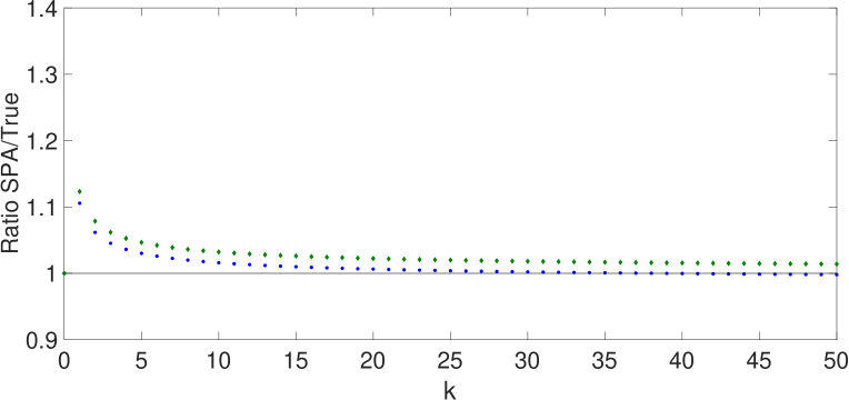
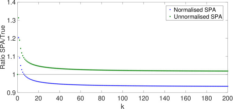
Figure 4.1: Ratio between the saddlepoint approximations and the exact probability mass function computed from (2.2) for the population size after $t=1$ in an LBDP with $\lambda=7$ and $\mu=5$ and initial population sizes $a=5$ (left) and $a=20$ (right).

$a$	$5$	$10$	$15$	$20$	$50$	$100$
SPA	5.9	5.7	5.9	6.0	6.3	6.9
Exact	138.9	188.6	312.3	413.7	1402.1	4939.7

Table 1: Average CPU time (ms, based on 100 runs, using Matlab on a 2.6 GHz Intel Core i5 laptop) to compute the saddlepoint approximation (SPA) and the exact probability mass function for population sizes $k=0,1,\ldots,200$ at $t=1$ in an LBDP with $\lambda=7$ and $\mu=5$, as a function of $Z(0)=a$.

Figure 4.1 shows that the ratio between the normalised and unnormalised saddlepoint approximations and the exact probability mass function converges to unity as the initial population sizes $a$ increases: the approximation improves as the numerical computation of the true distribution becomes more challenging. Table 1 compares the CPU times to compute the saddlepoint approximation $\tilde{p}_{k}(1;10)$ and the probability mass function ${p}_{k}(1;10)$ for $k=1$ to 200 and for some parameter values: in contrast with the saddlepoint approximation, the computational burden of the exact distribution increases with $Z(0)$.

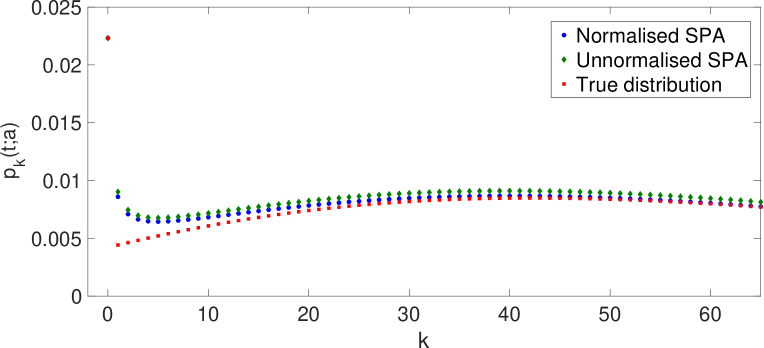
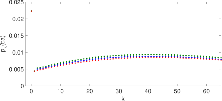
Figure 4.2: Probability mass function of the population size after $t=1$ in an LBDP with $\lambda=7$ and $\mu=5$ and initial population size $a=10$, together with its saddlepoint approximation $\tilde{p}_{k}(1;10)$ and the normalised saddlepoint approximation $\bar{p}_{k}(1;10)$. Left: unadjusted saddlepoint approximation; Right: conditional saddlepoint approximation.

The left-hand panel of Figure 4.2 shows that when there is a large gap between $p_{0}(t;a)$ and $p_{1}(t;a)$, the saddlepoint approximation has a smoothing effect around $k=0$, which decreases as $|p_{0}(t;a)-p_{1}(t;a)|$ decreases, i.e., as the initial population size $a$ increases. The smoothing can be adjusted by applying the saddlepoint technique to the conditional CGF, given that the population is not extinct at time $t$,

$$K\{x,t;a\,|\,Z(t)>0\}=\log\{M(x,t;a)-p_{0}(t;a)\}-\log\{1-p_{0}(t;a)\},$$

though the resulting saddlepoint $\tilde{x}(t,a,k)$ must be obtained numerically. The right-hand panel of Figure 4.2 shows the adjusted saddlepoint approximation. In practice, if $a$ and/or $k$ are large, this correction is not necessary.

The saddlepoint approximated log-likelihood is

$$\tilde{\ell}(\lambda,\mu;\bm{t},\bm{k})=\sum_{i=1}^{M}\sum_{j=1}^{N}\log\tilde{p}_{k_{i,j}}(\tau_{i,j};k_{i,j-1}),$$ (4.7)

where $\tau_{i,j}:=t_{i,j}-t_{i,j-1}$, and the values $\tilde{{\lambda}}$ and $\tilde{\mu}$ maximising this expression are called the saddlepoint maximum likelihood estimators (SPMLEs). We call this the SPMLE approach.

As indicated by Figure 4.1, the error of the saddlepoint approximation decreases as the initial population size $a$ increases; more precisely (see for example [9, Chapter 12]),

$${p}_{k}(t;a)=\tilde{p}_{k}(t;a)\{1+\mathcal{O}(1/a)\},$$ (4.8)

and this leads to the following lemma.

Lemma 2.

The error in the saddlepoint approximated log-likelihood is

$${\ell}(\lambda,\mu;\bm{t},\bm{k})-\tilde{\ell}(\lambda,\mu;\bm{t},\bm{k})=\mathcal{O}\left\{\left(\min_{1\leq i\leq M,1\leq j\leq N}\{k_{i,j-1}\}\right)^{-1}\right\}.$$

Proof.

We have

$${\ell}(\lambda,\mu;\bm{t},\bm{k})-\tilde{\ell}(\lambda,\mu;\bm{t},\bm{k}) = \sum_{i=1}^{M}\sum_{j=1}^{N}\log\{{p}_{k_{i,j}}(\tau_{i,j};k_{i,j-1})/\tilde{p}_{k_{i,j}}(\tau_{i,j};k_{i,j-1})\}$$

$$= \sum_{i=1}^{M}\sum_{j=1}^{N}\log\{1+\mathcal{O}(1/k_{i,j-1})\}\quad\mbox{by \eqref{err_spa}}$$

$$= \sum_{i=1}^{M}\sum_{j=1}^{N}\mathcal{O}(1/k_{i,j-1})$$

$$= \mathcal{O}\left\{\left(\min_{1\leq i\leq M,1\leq j\leq N}\{k_{i,j-1}\}\right)^{-1}\right\}.$$

∎

Every observed population size in every independent trajectory, except that for the last observation time, plays a role in the order of magnitude of the approximation error. For exploding trajectories where $k_{j,i}\geq k_{j,i-1}$, the error is dominated by the inverse population sizes $k_{j,0}$ at the first observation times, but for trajectories with a minimum population size close to zero, the error can become non-negligible. In this case, direct computation of the transition probabilities will be least onerous. Alternatively, it may be beneficial to use a multivariate version of the saddlepoint approximation, as described in the Appendix.

5 Gaussian approximations

Second-order Taylor expansion of the CGF $K(x,t;a)$ at $x=0$ yields

$$K(x,t;a)\approx xK^{\prime}(0,t;a)+\frac{x^{2}}{2}K^{\prime\prime}(0,t;a)=xm(t;a)+\frac{x^{2}}{2}\sigma^{2}(t;a),$$ (5.1)

and first-order Taylor expansion of $K^{\prime}(x,t;a)$ at $x=0$ yields

$$K^{\prime}(x,t;a)\approx K^{\prime}(0,t;a)+xK^{\prime\prime}(0,t;a)=m(t;a)+x\sigma^{2}(t;a).$$ (5.2)

Using (4.2) and (5.2), the saddle point $\tilde{x}(k,t;a)$ can be approximated as

$$\tilde{x}(k,t;a)\approx\dfrac{k-m(t;a)}{\sigma^{2}(t;a)},$$ (5.3)

and using (5.1) and (5.3), the exponent in (4.1) can be approximated as

$$K(\tilde{x},t;a)-\tilde{x}k \approx \tilde{x}\{m(t;a)-k\}+\dfrac{\tilde{x}^{2}}{2}\sigma^{2}(t;a)$$ (5.4)

$$\approx -\dfrac{\{k-m(t;a)\}^{2}}{2\sigma^{2}(t;a)}.$$ (5.5)

Thus the saddlepoint approximation to the conditional probability mass function is roughly

$$\tilde{\varphi}_{k}(t;a):=\left\{\dfrac{1}{2\pi\sigma^{2}(t;a)}\right\}^{1/2}\exp\left[-\dfrac{\{k-m(t;a)\}^{2}}{2\sigma^{2}(t;a)}\right],$$ (5.6)

i.e., the Gaussian density function with mean $m(t;a)$ and variance $\sigma^{2}(t;a)$.

This Gaussian approximation also arises from the central limit theorem. If $Z(0)=a$, then $Z(t)\overset{d}{=}\sum_{i=1}^{a}X_{i}(t)$, where the i.i.d. random variables $X_{i}(t)$ represent the population size in an LBDP that starts with a single individual at time zero, and have mean and variance $m(t;1)$ and $\sigma^{2}(t;1)$. By the central limit theorem, $Z(t)\overset{d}{\approx}\mathcal{N}\{am(t;1),a\sigma^{2}(t;1)\}=\mathcal{N}\{m(t;a),\sigma^{2}(t;a)\}$ for large values of $a$, so $p_{k}(t;a)\approx\tilde{p}_{k}(t;a)\approx\tilde{\varphi}_{k}(t;a)$. However, the saddlepoint approximation $\tilde{p}_{k}(t;a)$ retains much more information than the Gaussian approximation $\tilde{\varphi}_{k}(t;a)$, whose only ingredients are the first two moments of the population size.

We now establish a connection between the SPMLE and the GW approaches, and a natural extension of the latter to unequal inter-observation times. The proof of the next lemma can be found in Appendix A.

Lemma 3.

If the inter-observation times are equal within and between the trajectories, then the MLEs for $\lambda$ and $\mu$ resulting from (5.6) coincide with the GW estimators.

If the inter-observation times are unequal, then the approximation (5.6), in which $m(t;a)$ and $\sigma^{2}(t;a)$ are replaced by their expressions (2.3) and (2.6) in terms of $\lambda$, $\mu$, and the inter-observation times, can still be used to obtain estimators for $\lambda$ and $\mu$. Letting $\omega=\lambda-\mu$ and $\xi=\lambda+\mu$, the logarithm of (5.6) can be rewritten for any $t$ as

$$\log\tilde{\varphi}_{k}(t;a\,|\,(\omega,\xi)) = -\frac{1}{2}\log\{2\pi a(\xi/\omega)\exp(\omega t)[\exp(\omega t)-1]\}$$ (5.7)

$$-\dfrac{\omega\{k-a\exp(\omega t)\}^{2}}{2a\xi\exp(\omega t)\{\exp(\omega t)-1\}},$$

so (4.7) can be approximated by

$$\tilde{\tilde{\ell}}(\omega,\xi;\bm{t},\bm{k}) = -\frac{1}{2}\sum_{i=1}^{M}\sum_{j=1}^{N}\log\{2\pi k_{i,j-1}(\xi/\omega)\exp(\omega\tau_{i,j})[\exp(\omega\tau_{i,j})-1]\}$$ (5.8)

$$\quad-\frac{\omega}{2\xi}\sum_{i=1}^{M}\sum_{j=1}^{N}\dfrac{\{k_{i,j}-k_{i,j-1}\,\exp(\omega\tau_{i,j})\}^{2}}{k_{i,j-1}\exp(\omega\tau_{i,j})\{\exp(\omega\tau_{i,j})-1\}},$$

where $\tau_{i,j}=t_{i,j}-t_{i,j-1}$. The resulting MLEs generalise the GW estimators to unequal inter-observation times. The proof of the next theorem is provided in Appendix A.

Theorem 3.

Suppose that $M$ independent replicates of data are available from an LBDP with $\lambda>0$, potentially observed at times $0<t_{i,1}<\cdots<t_{i,N_{i}}$, where $N_{i}\geq 1$ and $t_{i,j}-t_{i,j-1}>\epsilon>0$ for $i=1,\ldots,M$ and all $j$. Suppose that observation for each replicate stops at the earlier of its extinction time $T_{i}$ and after $N_{i}$ observations, and that the conditional increments of the process have finite fourth moments almost surely. Then the estimators of $\lambda$ and $\mu$ resulting from maximisation of (5.8) are consistent and asymptotically normally distributed as $M\to\infty$, with covariance matrix given in (7.10).

6 Simulations

To compare the SPMLE with the MLE, we simulated independent non-extinct trajectories of LBDPs with $\lambda=7$ and $\mu=5$, with various initial population sizes. For each trajectory, we recorded the population sizes at $N+1=20$ time points and used them to calculate the SPMLE and MLE. In about a fifth of the trajectories the observed population size exceeded 600 individuals and the MLE could not be computed. The relative error was never greater than 5%, and only exceeded 2% for minimum population sizes smaller than 5. The relative error for $\omega$ is generally smaller than 0.01%, so the saddlepoint approximation errors in the SPMLEs of $\lambda$ and $\mu$ appear to cancel for $\hat{\lambda}-\hat{\mu}$. The maximum observed population size has no impact on the CPU time necessary to compute the SPMLE, which was around 0.1s in each case, whereas the CPU time to obtain the exact MLE increases roughly linearly with the population size at rate around 0.2 s/individual.

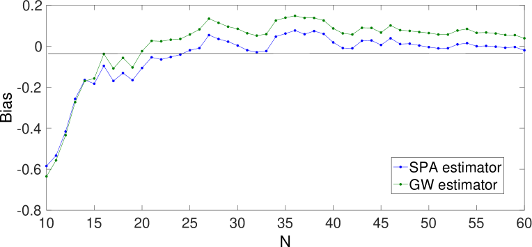
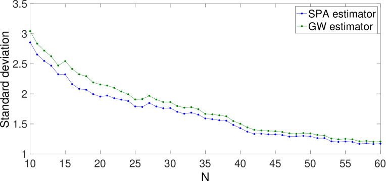
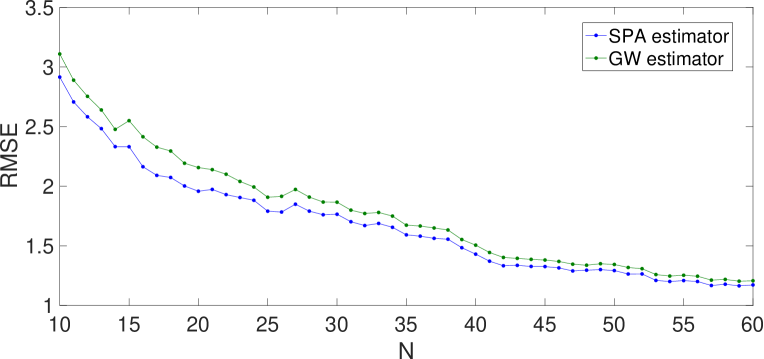
We ran a series of simulation experiments, either increasing the number $N$ of discrete-time observations, or increasing the number $M$ of independent observed trajectories. We first simulated 100 replicates of a single ($M=1$) non-extinct trajectory of an LBDP with $\lambda=7$ and $\mu=6$, starting with $Z(0)=10$ individuals, and we computed the bias, standard deviation and root mean square error (RMSE) of $\hat{\lambda}$ and $\hat{\omega}$ for $N=10,\ldots,60$. Figure 6.1 depicts the results for $\hat{\lambda}$. Both biases decrease rapidly as $N$ increases, with the SPMLE having smaller bias than the GW estimator. The gap between the standard deviation and RMSE of the GW and SPMLE estimator decreases as $N$ increases.

Figure 6.1: Properties of $\hat{\lambda}$ as $N$ increases: Bias, standard deviation and root mean square error for an LBDP with $\lambda=7,\mu=6$, $Z(0)=Z_{0}=10$. Results based on 100 simulations of a single ($M=1$) non-extinct trajectory observed $N+1$ times, at constant inter-observation times $\Delta t=0.07$.

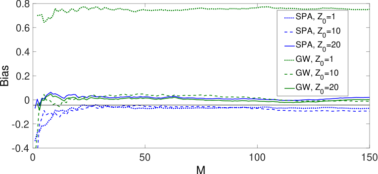
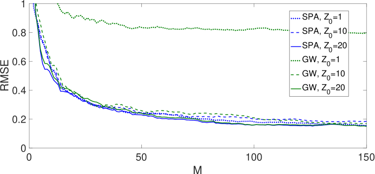
In a second experiment, we fix $N=30$ and analyse properties of the estimators for $M=1,\ldots,150$, for an LBDP with $\lambda=7$ and $\mu=5$ starting with different initial population sizes $Z(0)=Z_{0}=1,10,20$. The bias and RMSE of $\hat{\lambda}$ are presented in Figure 6.2. The quality of the estimators improves rapidly as $M$ increases. The value of $Z_{0}$ has a clear impact on the quality of the GW estimator, and less impact on that of the SPMLE. We further investigate the effect of $Z_{0}$ in the RMSE of both estimators for different values of $N$, $M$, and the model parameters. We summarise the results in Table 2, which confirms the key role played by $Z_{0}$ in the quality of the GW estimator, which becomes comparable to the SPMLE as $Z_{0}$ increases. For the same value of $M,N$ and $Z_{0}$, the quality of the estimators increases as the process moves away from criticality ($\omega=0$), as suggested when $m\to 1$ in Theorem 1.

Figure 6.2: Properties of $\hat{\lambda}$ as $M$ increases: Bias and root mean square error for an LBDP with $\lambda=7,\mu=5$, $Z(0)=Z_{0}=1,10,20$. Results based on 100 simulations of $M$ non-extinct trajectories observed $N+1=30$ times at constant inter-observation times $\Delta t=1/10$.

$M=1$, $\mu=6$, $\omega=1$

	$Z_{0}=1$	$Z_{0}=5$	$Z_{0}=10$	$Z_{0}=20$	$Z_{0}=50$
SPMLE	2.40	2.44	2.40	2.45	2.48
GW	5.03	3.38	2.82	2.68	2.56

$M=1$, $\mu=5$, $\omega=2$         $M=20$, $\mu=5$, $\omega=2$

	$Z_{0}=1$	$Z_{0}=5$	$Z_{0}=10$	$Z_{0}=20$	$Z_{0}=1$	$Z_{0}=5$	$Z_{0}=10$	$Z_{0}=20$
SPMLE	1.63	1.59	1.57	1.71	0.39	0.35	0.35	0.36
GW	2.15	1.75	1.64	1.62	0.62	0.40	0.36	0.36

Table 2: Root mean square error of $\hat{\lambda}$ (true value $\lambda=7$) based on 5000 simulations of $M$ non-extinct trajectories observed $N+1=30$ times at constant inter-observation times $\Delta t=1/10$ for different values of $Z_{0}$.

7 Applications

We use the GW and MLE approaches to estimate the birth and death rates in two bird populations and the transmission and removal rates for an influenza epidemic. In each case a single trajectory ($M=1$) of the population is observed at equally-spaced times.

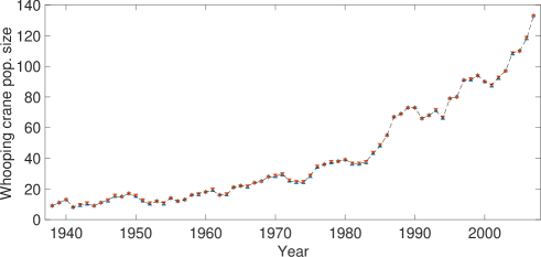
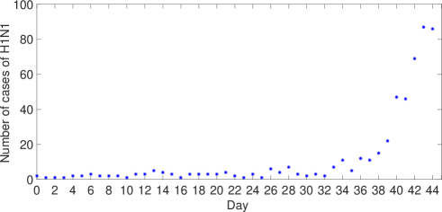
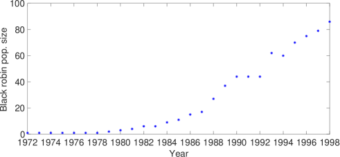
Figure 7.1: Data for examples. Top: Yearly black robin population census, 1972–1998, corresponding to females who survived up to at least one year. Middle: Yearly population census of the young and adult whooping cranes arriving in Texas each autumn, 1938–2007. Counts correspond to the number of females, obtained by dividing the total size by two (assuming a 1:1 sex ratio), and are rounded up ($\blacktriangledown$) or down ($\blacktriangle$) when the value is non-integer. The black line represents a uniform choice between the upper and lower values, which forms our data. Bottom: Daily counts ($+1$) of new cases during the H1N1 outbreak in Mexico from 11 March 2009 (Day 0) to 24 April 2009 (Day 44).

7.1 Black robin population

The black robin Petroica traversi is an endangered songbird species endemic to the Chatham Islands. By 1980, the population had declined to five birds, including only one successful breeding pair [12]. Through intensive conservation efforts in 1980–1989 by the New Zealand Wildlife Service (now the Department of Conservation), the population recovered to 93 birds by spring 1990 [20, 22]. Over the next decade (1990–1998), the population was closely monitored, but without human intervention, and grew to 197 adults by 1998 [19]. After this period its growth slowed considerably and it only reached 239 adults in 2011 [23] and 298 in 2014.

We fit an LBDP to the yearly censuses of the female black robin population between 1972 and 1998 ($N=26$). The data are presented in Figure 7.1, and the estimates are shown in Table 3. Due to relatively large population sizes, obtaining the MLE was numerically problematic. The computation of the GW estimators is 305 times faster than for the SPMLEs, whose computation is iteself 167 times faster on average than the MLEs. The GW estimates are very close to the MLEs, but the SPMLEs are a little different owing to small population sizes in the early years. The adjusted SPMLEs (correcting for the smoothing effect around small population sizes) show a substantial improvement.

We conclude that a one-year-old female bird has a life expectancy of $1/0.19=5.26$ years and gives birth on average to $0.318/0.19=1.67$ female offspring reaching an age of one year; these are reasonable estimates. Assuming constant birth and death rates, the estimated probability of extinction for the black robin is $0.19/0.318=0.6$ (SE $0.018$).

	GW estimates	SPMLE	Adjusted SPMLE	MLE
$\hat{\lambda}$	0.319 (0.071)	0.301 (0.073)	0.319 (0.072)	0.318 (0.072)
$\hat{\mu}$	0.191 (0.071)	0.173 (0.072)	0.191 (0.071)	0.190 (0.071)
$\hat{\omega}$	0.128 (0.028)	0.128 (0.027)	0.128 (0.028)	0.128 (0.028)
CPU time (sec)	$2.67\,10^{-4}$	0.081	1.35	13.61

Table 3: Estimates (and standard errors based on Theorem 1 for the GW estimates, and on Fisher Information for the SPMLE and the MLE) of the birth, death, and growth rates of the black robin population between 1972 and 1998 from the GW, SPMLE and MLE approaches, and average CPU times.

7.2 Whooping crane population

The whooping crane is a rare migratory bird that breeds in northern Canada and winters in Texas. Stratton [28] provides annual counts of whooping cranes arriving in Texas during autumn from 1938–2007 ($N=69$). LBDPs were used to model their population between 1938 and 1972 in Miller et al. [24] and in Guttorp [15, p.47], but as the original dataset includes both males and females, dependences and mating make it unlikely that an LBDP fits properly. We therefore model the female population only, assuming a sex ratio of 1:1; see Figure 7.1, and Table 4. Again due to relatively large population sizes, the computation of the MLEs caused numerical issues. The SPMLEs are closer to the MLEs than to the GW estimates. The adjusted SPMLE gives no strong improvement because the population sizes are not close to zero. The estimated birth and death rates seem more realistic than those obtained in [15] and give an estimated extinction probability of $0.149/0.193=0.772$ (SE $0.002$).

	GW estimates	SPMLE	Adjusted SPMLE	MLE
$\hat{\lambda}$	0.186 (0.023)	0.195 (0.031)	0.195 (0.030)	0.193 (0.030)
$\hat{\mu}$	0.142 (0.023)	0.152 (0.031)	0.152 (0.030)	0.149 (0.030)
$\hat{\omega}$	0.044 (0.011)	0.044 (0.011)	0.044 (0.011)	0.043 (0.011)

Table 4: Estimates (and standard errors computed as in Table 3) of the birth, death, and growth rates of the whooping crane female population.

7.3 H1N1 influenza outbreak

Finally, we apply our methods to the initial stage of the H1N1 pandemic in 2009 in Mexico, using daily counts of new cases reported between the outbreak on 11 March and 24 April, when educational institutions in Mexico City were shut ($N=44$) [13]. See Figure 7.1 and Table 5. The SPMLEs are again closer to the MLEs than are the GW estimates, and adjusting for the smoothing effect again improves the result considerably. The estimated basic reproduction number is $\hat{R}_{0}=0.841/0.658\approx 1.28>1$, consistent with the Bayesian results of Fraser et al. [13]. The estimated Malthusian parameter, $0.044$, is lower than the estimate of $0.199$ obtained by Kraus and Panaretos [21] under the assumption of under-reporting. We estimate the expected length of the infectious period to be $1/0.15\approx 6.67$ days, which appears reasonable, since it is believed to be until five to seven days after the symptoms appear.

	GW estimates	SPMLE	Adjusted SPMLE	MLE
$\hat{\lambda}$	1.067 (0.208)	0.952 (0.190)	0.883 (0.139)	0.841 (0.144)
$\hat{\mu}$	0.884 (0.208)	0.770 (0.189)	0.701 (0.140)	0.658 (0.143)
$\hat{\omega}$	0.182 (0.065)	0.182 (0.061)	0.182 (0.059)	0.182 (0.057)

Table 5: Estimates (and standard errors computed as in Table 3) of the birth (transmission), death (removal), and growth rates of the population infected by H1N1.

References

• [1] Y. Aı and J. Yu. Saddlepoint approximations for continuous-time Markov processes. Journal of Econometrics, 134(2):507–551, 2006.
• [2] R.W. Butler. Saddlepoint Approximations with Applications, volume 22. Cambridge University Press, 2007.
• [3] R. Chen and O. Hyrien. Quasi-and pseudo-maximum likelihood estimators for discretely observed continuous-time markov branching processes. Journal of Statistical Planning and Inference, 141(7):2209–2227, 2011.
• [4] F.W. Crawford, V.N. Minin, and M.A. Suchard. Estimation for general birth-death processes. Journal of the American Statistical Association, 109(506):730–747, 2014.
• [5] F.W. Crawford and M.A. Suchard. Transition probabilities for general birth–death processes with applications in ecology, genetics, and evolution. Journal of Mathematical Biology, 65(3):553–580, 2012.
• [6] H.E. Daniels. Saddlepoint approximations in statistics. The Annals of Mathematical Statistics, pages 631–650, 1954.
• [7] H.E. Daniels. The saddlepoint approximation for a general birth process. Journal of Applied Probability, 19(1):20–28, 1982.
• [8] J.H. Darwin. The behaviour of an estimator for a simple birth and death process. Biometrika, 43(1/2):23–31, 1956.
• [9] A.C. Davison. Statistical Models, volume 11. Cambridge University Press, 2003.
• [10] J.P. Dion and N.M. Yanev. Statistical inference for branching processes with an increasing random number of ancestors. Journal of Statistical Planning and Inference, 39(2):329 – 351, 1994.
• [11] C. Duby and A. Rouault. Estimation non paramétrique de l’espérance et de la variance de la loi de reproduction d’un processus de ramification. Annales de l’Institut Henry Poincaré, XVIII Section B, 18(2):149–163, 1982.
• [12] E.P. Elliston. The black robin: Saving the world’s most endangered bird. BioScience, 44(7):499–501, 1994.
• [13] C. Fraser, C. A. Donnelly, S. Cauchemez, W. P. Hanage, M. D. Van Kerkhove, T. D. Hollingsworth, J. Griffin, R. F. Baggaley, H. E. Jenkins, E. J. Lyons, et al. Pandemic potential of a strain of influenza A (H1N1): early findings, Science, 324(5934), 1557–1561, 2009.
• [14] G. R. Grimmett and D. R. Stirzaker. Probability and Random Processes, third edn, Clarendon Press, Oxford, 2001.
• [15] P. Guttorp. Statistical Inference for Branching Processes. Wiley, New York, 1991.
• [16] T.E. Harris. The Theory of Branching Processes. Courier Corporation, 2002.
• [17] S. Karlin and H.M. Taylor. A first course in stochastic processes academic. New York, 1975.
• [18] N. Keiding. Maximum likelihood estimation in the birth-and-death process. Annals of Statistics, 3(2):363–372, 1975.
• [19] E. S. Kennedy. Extinction vulnerability in two small, chronically inbred populations of Chatham Island black robin petroica traversi, PhD thesis, Lincoln University, New Zealand, 2009.
• [20] E.S. Kennedy, C.E. Grueber, R.P. Duncan, and I.G. Jamieson. Severe inbreeding depression and no evidence of purging in an extremely inbred wild species – the Chatham Island black robin. Evolution, 68(4):987– 995, 2014.
• [21] A. Kraus and V. M. Panaretos. Frequentist estimation of an epidemic’s spreading potential when observations are scarce., Biometrika 101(1), 141–154, 2014.
• [22] M. Massaro, R. Sainudiin, D. Merton, J. V. Briskie, J. V., A. M. Poole, and M. L. Hale. Human-assisted spread of a maladaptive behavior in a critically endangered bird, PloS one 8(12), e79066, 2013.
• [23] M. Massaro, M. Stanbury, and J.V. Briskie. Nest site selection by the endangered black robin increases vulnerability to predation by an invasive bird. Animal Conservation, 16(4):404–411, 2013.
• [24] R. S. Miller, D. B. Botkin,and R. Mendelssohn. The whooping crane (Grus americana) population of North America, Biological Conservation 6(2), 106–111, 1974.
• [25] A.S. Novozhilov, G.P. Karev, and E.V. Koonin. Biological applications of the theory of birth-and-death processes. Briefings in bioinformatics, pages 70–85, 2006.
• [26] X. Pedeli, A.C. Davison, and K. Fokianos. Likelihood estimation for the INAR(p) model by saddlepoint approximation. Journal of the American Statistical Association, 110(511):1229–1238, 2015.
• [27] J.V. Ross, T. Taimre, and P.K. Pollett. On parameter estimation in population models. Theoretical Population Biology, 70(4):498–510, 2006.
• [28] D. A. Stratton. Case Studies in Ecology and Evolution, Technical report, University of Vermont. Draft of a coming textbook, 2016.
• [29] A. W. van der Vaart, Asymptotic Statistics, Cambridge University Press, Cambridge, 1998.
• [30] J. Xu, P. Guttorp, M. Kato-Maeda, and V.N. Minin. Likelihood-based inference for discretely observed birth–death-shift processes, with applications to evolution of mobile genetic elements. Biometrics, 71(4):1009–1021, 2015.