Quantum phase transitions of a two-leg bosonic ladder in an artificial gauge field

Abstract

We consider a two leg bosonic ladder in a $U(1)$ gauge field with both interleg hopping and interleg repulsion. As a function of the flux, the interleg interaction converts the commensurate-incommensurate transition from the Meissner to a Vortex phase, into an Ising-type of transition towards a density wave phase. A disorder point is also found after which the correlation functions develop a damped sinusoid behavior signaling a melting of the vortex phase. We discuss the differences on the phase diagram for attractive and repulsive interleg interaction. In particular, we show how repulsion favors the Meissner phase at low-flux and a phase with a second incommensuration in the correlation functions for intermediate flux, leading to a richer phase diagram than in the case of interleg attraction. The effect of the temperature on the chiral current is also discussed.

I introduction

Trapped ultracold atoms have provided experimentalists with a unique ability to realize highly tunable quantum simulators of many-body model Hamiltonians,Jaksch and Zoller (2005); Lewenstein et al. (2007); Bloch et al. (2008) including quasi-one dimensional systems.Cazalilla et al. (2011) Moreover, it has recently become possible to simulate the effect of an applied magnetic field using two-photon Raman transitionsLin et al. (2011); Dalibard et al. (2011); Galitski and Spielman (2013), spin-orbit couplingCeli et al. (2014) or optical clock transitionsLivi et al. (2016). Such situation gives access to a regime where the interplay of low dimensionality, interaction and magnetic field generates exotic phases such as bosonic analogues of the Fractional Quantum Hall Effect.Regnault and Jolicoeur (2003) The simplest system to observe nontrivial effects of an artificial gauge field is the bosonic two-leg ladder.Atala et al. (2014) Originally, such systems were considered in the context of Josephson junction arrays in magnetic fieldKardar (1986); Orignac and Giamarchi (2001a); Cha and Shin (2011) and a commensurate-incommensurate (C-IC) phase transition between a Meissner-like phase with currents along the legs and a Vortex-like phase with quasi long range ordered current loops was predicted. However, in Josephson junction systems, ohmic dissipationAmbegaokar et al. (1982); Korshunov (1989) spoiled the quantum coherence required to observe such transition. In cold atom systems, the Meissner and Vortex states have been observed in a non-interacting case.Atala et al. (2014) Moreover, recent progress in superconducting qbitsRoushan et al. (2017) engineering offer another promising pathLe Hur et al. (2016); Romero et al. (2017) for realization of low dimensional bosons in artificial flux. The availability of experimental systems has thus renewed theoretical interest in the two leg bosonic ladder in a fluxDhar et al. (2012, 2013); Petrescu and Le Hur (2013); Po et al. (2014); Xu et al. (2014); Zhao et al. (2014); Wei and Mueller (2014); Hügel and Paredes (2014); Piraud et al. (2014, 2015); Keleş and Oktel (2015); Greschner et al. (2015, 2016); Petrescu and Le Hur (2015); Barbiero et al. (2016); Peotta et al. (2014); Di Dio et al. (2015); Orignac et al. (2016); Petrescu et al. (2016); Barbarino et al. (2016); Strinati et al. (2017); Tokuno and Georges (2014); Uchino and Tokuno (2015); Bilitewski and Cooper (2016); Greschner and Vekua (2017); Guo and Poletti (2017); Richaud and Penna (2017); Romen and Läuchli (2017). These works have revealed in that deceptively simple model a zoo of ground state phases besides Meissner-like and Vortex-like ones. At commensurate filling, Mott-Meissner and Mott-Vortex phasesPiraud et al. (2015) as well as chiral Mott insulating phasesDhar et al. (2012, 2013); Petrescu and Le Hur (2013); Romen and Läuchli (2017) have been predicted. Meanwhile, with strong repulsion and a flux $\Phi=2\pi n$ with $n$ the number of particles per rung, bosonic analogs of the Laughlin statesLaughlin (1983) are expected Petrescu and Le Hur (2015); Petrescu et al. (2016); Strinati et al. (2017). Interactions also affect the C-IC transition between the Meissner-like and the Vortex-like phaseNatu (2015). In a previous workOrignac et al. (2017), we have considered the effect of attractive interchain interactions on the C-IC transition. Using an analogy with statistical mechanics of classical elastic systems on periodic substratesBohr et al. (1982); Bohr (1982); Haldane et al. (1983); Schulz (1983); Horowitz et al. (1983), we showed that interchain attraction split the single commensurate-incommensurate (C-IC) transition point into (a) an Ising transition point between the Meissner-like phase and a density-wave phase, (b) a disorder pointStephenson (1970a, b) where incommensuration develops inside the density-wave phase, and (c) a Berezinskii-Kosterlitz-Thouless (BKT) transitionBerezinskii (1971); Kosterlitz and Thouless (1973) where the density wave with incommensuration turns into the Vortex-like phase. The density wave phase with incommensuration can be identified as a melted vortex state while the transition (c) can be seen as a melting of the vortex phase. The density wave competing with the Meissner phase at Ising point (a) is induced by interchain interactionCazalilla and Ho (2003); Mathey et al. (2000); Hu et al. (2009) even in the absence of flux. We have verified the existence of those phases in DMRG simulations of hard core bosons.Orignac et al. (2017) Since the analogy with classical elastic systems holds irrespective of the sign of the interchain interaction, a similar splitting of the C-IC point should also in the repulsive case. In the present manuscript, we show that the splitting, if present, must occur in a much narrower region of flux than in the attractive case.

The paper is organized as follows: In Section II we introduce the model and its bosonized version, here we also introduce the observables and their correlation functions. In Section III we discuss the Ising transition and the disorder point by using a fermionization approach based on the Majorana fermion representation. Here we also briefly discuss the effect of the temperature on the spin current and momentum distribution. In Section IV we discuss the emergence of the second incommensuration by using a unitary transformation approach and non-abelian bosonization. Section V presents the numerical results for the hard-core limit in the legs. In Section VI we discuss the major results and give some conclusions.

II Model

We consider a model of bosons on a two-leg ladder in the presence of an artificial U(1) gauge fieldBarbarino et al. (2016); Strinati et al. (2017):

$$H=-t\sum_{j,\sigma}(b^{\dagger}_{j,\sigma}e^{i\lambda\sigma}b_{j+1,\sigma}+b^{\dagger}_{j+1,\sigma}e^{-i\lambda\sigma}b_{j,\sigma})$$

$$+\frac{\Omega}{2}\sum_{j,\alpha,\beta}b^{\dagger}_{j,\alpha}(\sigma^{x})_{\alpha\beta}b_{j,\beta}+\sum_{j,\alpha,\beta}U_{\alpha\beta}n_{j\alpha}n_{j\beta},$$ (1)

where $\sigma=\uparrow,\downarrow$ represents the leg index, $b_{j,\sigma}$ annihilates a boson on leg $\sigma$ on the $j-$th site, $n_{j\alpha}=b^{\dagger}_{j\alpha}b_{j\alpha}$, $t$ is the hopping amplitude along the chain, $\Omega$ is the tunneling between the legs, $\lambda$ is the Peierls phase of the effective magnetic field associated to the gauge field, $U_{\uparrow\uparrow}=U_{\downarrow\downarrow}$ is the repulsion between bosons on the same leg, $U_{\downarrow\uparrow}=U_{\perp}$ the interaction between bosons on opposite legs. This model can be mapped to a spin-1/2 bosons with spin-orbit interaction modelOrignac et al. (2016), where $\Omega$ is the transverse magnetic field, $\lambda$ measures the spin-orbit coupling, $U_{\uparrow\uparrow}=U_{\downarrow\downarrow}$ is the repulsion between bosons of identical spins, $U_{\downarrow\uparrow}=U_{\perp}$ the interaction between bosons of opposite spins.

II.1 Bosonized description

Let us derive the low-energy effective theory for the Hamiltonian (II), treating $\Omega$ and $U_{\perp}$ as perturbations, and using Haldane’s bosonization of interacting bosons.Haldane (1981)

IntroducingHaldane (1981) the fields $\phi_{\alpha}(x)$ and $\Pi_{\alpha}(x)$ satisfying canonical commutation relations $[\phi_{\alpha}(x),\Pi_{\beta}(y)]=i\delta(x-y)$ as well as the dual $\theta_{\alpha}(x)=\pi\int^{x}dy\Pi_{\alpha}(y)$ of $\phi_{\alpha}(x)$, we can represent the boson annihilation operators as:

$$\frac{b_{j\sigma}}{\sqrt{a}}=\psi_{\sigma}(x)=e^{i\theta_{\sigma}(x)}\sum_{m=0}^{+\infty}A^{(\sigma)}_{m}\cos(2m\phi_{\sigma}(x)-2m\pi\rho^{(0)}_{\sigma}x),$$ (2)

and the density operatorsHaldane (1981) as:

$$\frac{n_{j\sigma}}{a} = \rho_{\sigma}(x)=\rho_{\sigma}^{(0)}-\frac{1}{\pi}\partial_{x}\phi_{\sigma}$$ (3)

$$+ \sum_{m=1}^{\infty}B_{m}^{(\sigma)}\cos(2m\phi_{\sigma}(x)-2m\pi\rho^{(0)}_{\sigma}x).$$

Here, we have introduced the lattice spacing $a$, while $A_{m}$ and $B_{m}$ are non-universal coefficients that depend on the microscopic details of the model. For integrable models, these coefficients have been determined from Bethe Ansatz calculationsLukyanov and Terras (2003); Ovchinnikov (2004); Shashi et al. (2012) while for non-integrable models, they can be determined from numerical calculations of correlation functions.Hikihara and Furusaki (2003); Bouillot et al. (2011)

Introducing the canonically conjugate linear combinations:

$$\phi_{c}=\frac{1}{\sqrt{2}}(\phi_{\uparrow}+\phi_{\downarrow})\;\;\Pi_{c}=\frac{1}{\sqrt{2}}(\Pi_{\uparrow}+\Pi_{\downarrow}),$$ (4)

$$\phi_{s}=\frac{1}{\sqrt{2}}(\phi_{\uparrow}-\phi_{\downarrow})\;\;\Pi_{s}=\frac{1}{\sqrt{2}}(\Pi_{\uparrow}-\Pi_{\downarrow}),$$ (5)

the bosonized Hamiltonian can be rewritten as $H=H_{c}+H_{s}$, where

$$H_{c}=\int\frac{dx}{2\pi}\left[u_{c}K_{c}(\pi\Pi_{c})^{2}+\frac{u_{c}}{K_{c}}(\partial_{x}\phi_{c})^{2}\right]$$ (6)

describes the total density fluctuations for incommensurate filling when umklapp terms are irrelevant, and

$$H_{s}=\int\frac{dx}{2\pi}\left[u_{s}K_{s}\left(\pi\Pi_{s}+\frac{\lambda}{a\sqrt{2}}\right)^{2}+\frac{u_{s}}{K_{s}}(\partial_{x}\phi_{s})^{2}\right]$$

$$-2\Omega A_{0}^{2}\int dx\cos\sqrt{2}\theta_{s}+\frac{U_{\perp}aB_{1}^{2}}{2}\int dx\cos\sqrt{8}\phi_{s}$$ (7)

describes the antisymmetric density fluctuations. In Eq. (7) and  (6), $u_{s}$ and $u_{c}$ are respectively the velocity of antisymmetric and total density excitations, $A_{0}$ and $B_{1}$ are non universal coefficientsGiamarchi (2004) while $K_{s}$ and $K_{c}$ are corresponding the Tomonaga-Luttinger (TL) exponents. They can be expressed as a function of the velocity of excitations $u$, and Tomonaga-Luttinger liquid exponent $K$ of the isolated chain as:

$$u_{c}=u\left(1+\frac{U_{\perp}Ka}{\pi u}\right)^{1/2}$$ (8)

$$u_{s}=u\left(1-\frac{U_{\perp}Ka}{\pi u}\right)^{1/2}$$ (9)

$$K_{c}=K\left(1+\frac{U_{\perp}Ka}{\pi u}\right)^{-1/2}$$ (10)

$$K_{s}=K\left(1-\frac{U_{\perp}Ka}{\pi u}\right)^{-1/2}$$ (11)

For an isolated chain of hard core bosons, we have $u=2t\sin(\pi\rho^{0}_{\sigma})$ and $K=1$. Physical observables can also be represented in bosonization. The rung current, or the flow of bosons from the upper leg to the lower leg, is:

$$J_{\perp}(j) = -i\Omega(b^{\dagger}_{j,\uparrow}b_{j_{\downarrow}}-b^{\dagger}_{j,\downarrow}b_{j_{\uparrow}}).$$ (12)

$$= 2\Omega A_{0}^{2}\sin\sqrt{2}\theta_{s}+\ldots$$

The chiral current, i.e. the difference between the currents of upper and lower leg, is defined as

$$J_{\parallel}(j,\lambda) = -it\sum_{\sigma}\sigma(b^{\dagger}_{j,\sigma}e^{i\lambda\sigma}b_{j+1,\sigma}-b^{\dagger}_{j+1,\sigma}e^{-i\lambda\sigma}b_{j,\sigma}),$$ (13)

$$= \frac{u_{s}K_{s}}{\pi\sqrt{2}}\left(\partial_{x}\theta_{s}+\frac{\lambda}{a\sqrt{2}}\right).$$ (14)

The density difference between the chains $S_{j}^{z}=n_{j\uparrow}-n_{j\downarrow}$, is written in bosonization as:

$$S_{j}^{z}=-\frac{\sqrt{2}}{\pi}\partial_{x}\phi_{s}-2B_{1}\sin(\sqrt{2}\phi_{c}-\pi\rho x)\sin\sqrt{2}\phi_{s},$$ (15)

while the density of particles per rung is:

$$n_{j}=-\frac{\sqrt{2}}{\pi}\partial_{x}\phi_{c}-2B_{1}\cos(\sqrt{2}\phi_{c}-\pi\rho x)\cos\sqrt{2}\phi_{s}.$$ (16)

Let us discuss some simple limits of the Hamiltonian (7). When $\Omega\neq 0$, $U_{\perp}=0$, and $\lambda\rightarrow 0$, the antisymmetric modes Hamiltonian Eq. (7) reduces to a quantum sine-Gordon Hamiltonian. For $K_{s}>1/4$, the spectrum of $H_{s}$ is gapped and the system is in the so-called Meissner stateKardar (1986); Orignac and Giamarchi (2001a) characterized by $\langle\theta_{s}\rangle=0$. In such state, the chiral current increases linearly with the applied flux at small $\lambda$, while the average rung current $\langle J_{\perp}\rangle=0$ and its correlations $\langle J_{\perp}(j)J_{\perp}(0)\rangle$ decay exponentially with distance. The antisymmetric density correlations also decay exponentially with distance, while the symmetric ones behave as:

$$\langle n_{i}n_{j}\rangle=-\frac{2K_{c}}{\pi^{2}(i-j)^{2}}+e^{-|i-j|/\xi}\frac{\cos\pi n(i-j)}{|i-j|^{K_{c}}},$$ (17)

where $\xi$ is the correlation length resulting from the spectral gap of $H_{s}$. With $\Omega=0,U_{\perp}\neq 0$, the antisymmetric density fluctuations Hamiltonian (7) becomes again a quantum sine-Gordon model that can be related to the previous one by the duality transformation $\theta_{s}\to 2\phi_{s},\phi_{s}\to\theta_{s}/2,K_{s}\to 1/(4K_{s})$. For $K_{s}<1$, the Hamiltonian $H_{s}$ has a gapped spectrum and $\langle\phi_{s}\rangle=\frac{\pi}{\sqrt{8}}$ for $U_{\perp}>0$ yielding a zig-zag density wave ground state and $\langle\phi_{s}\rangle=0$ for $U_{\perp}<0$ yielding a rung density wave ground state.Orignac and Giamarchi (1998); Cazalilla and Ho (2003); Mathey (2007); Mathey and Wang (2007); Mathey et al. (2009); Hu et al. (2009) In both density wave states, the expectation values of the spin and conversion current vanish, and their correlations decay exponentially. The Green’s functions of the bosons also decay exponentially, so that the momentum distribution only has a Lorentzian shaped maximum at $k=0$. However, in the zig-zag density wave state ($U_{\perp}>0)$, we have:

$$\langle S_{j}^{z}S_{k}^{z}\rangle \sim C_{1}e^{-|j-k|/\xi}+C_{2}\frac{\cos\pi n(j-k)}{|j-k|^{K_{c}}},$$ (18)

$$\langle n_{j}n_{k}\rangle \sim -\frac{2K_{c}}{\pi^{2}(j-k)^{2}}+C_{3}\frac{\cos\pi n(j-k)}{|j-k|^{K_{c}}}e^{-|j-k|/\xi},$$ (19)

while in the rung density wave ($U_{\perp}<0$),

$$\langle n_{j}n_{k}\rangle \sim -\frac{2K_{c}}{\pi^{2}(j-k)^{2}}+C^{\prime}_{3}\frac{\cos\pi n(j-k)}{|j-k|^{K_{c}}},$$ (20)

$$\langle S_{j}^{z}S_{k}^{z}\rangle \sim C^{\prime}_{1}e^{-|j-k|/\xi}+C^{\prime}_{2}\frac{\cos\pi n(j-k)}{|j-k|^{K_{c}}}e^{-|j-k|/\xi}$$ (21)

where $K_{c}$ depends on the interleg interaction, increasing when it is attractive and decreasing when it is repulsive as indicated in Eq. (8). The behavior of density correlations in real space is reflected in the corresponding static structure factors:

$$S^{c}(q)=\sum_{j}e^{-iqj}\langle n_{j}n_{0}\rangle,$$ (22)

$$S^{s}(q)=\sum_{j}\langle S_{j}^{z}S_{0}^{z}\rangle.$$ (23)

In all phases, $S^{c}(q\to 0)=\frac{2K_{c}}{\pi}|q|+o(q)$, while $S_{s}(q)\sim S_{s}(0)+Aq^{2}+o(q^{2})$ indicating that symmetric excitations are always gapless while antisymmetric excitations are always gapped. However, in the rung density wave, $S_{c}(q\to\pi n)$ has a power law divergence $\sim|q-\pi n|^{K_{c}-1}$ (if $K_{c}<1$) or a cusp $\sim C+C^{\prime}|q-\pi n|^{K_{c}-1}$ (if $1<K_{c}<2$) and $S_{s}(q\to\pi n)$ has only a Lorentzian-shaped maximum while in the zig-zag density-wave, $S_{s}(q\to\pi n)$ shows a cusp or singularity while $S_{c}(q\to\pi n)$ has a Lorentzian-shaped maximum. The case of $U_{\alpha\alpha}=+\infty$ is peculiar as $K_{s}\to 1$. The Hamiltonian (II) can then be mapped to the Fermi-Hubbard model (see Sec. A.2). Bosonization of the Fermi-Hubbard modelGiamarchi (2004) shows that the operator $\cos\sqrt{8}\phi_{s}$ is marginal in the renormalization group sense. On the attractive side,Giamarchi (2004) it is marginally relevant, and the density wave exists for all $U_{\perp}<0$. However, on the repulsive side, $\cos\sqrt{8}\phi_{s}$ is marginally irrelevant and the staggered density wave is absent.

With both $\Omega$ and $U_{\perp}$ nonzero and $\lambda=0$, the Hamiltonian $H_{s}$ becomes the self-dual sine-Gordon model.José et al. (1977); Lecheminant et al. (2002) When both cosines are relevant (i. e. $1/4<K_{s}<1$) the Meissner phase (stable for $|\Omega|\gg|U_{\perp}|$) is competing with the density wave phases (stable in the opposite limit). The competing phases are separated by an Ising critical point.José et al. (1977); Lecheminant et al. (2002) In the case of $U_{\alpha\alpha}=+\infty$, since the density wave is absent for $U_{\perp}>0$, one only has the Meissner state for all $U_{\perp}>0$. By contrast, for $U_{\perp}<0$, the charge density wave exists at $\Omega=0$ and an Ising critical point is present. Thus, phase diagrams for $U_{\perp}>0$ and $U_{\perp}<0$ are very different.

In the presence of flux ($\lambda\neq 0$), the density wave phases are stable. However,for $U_{\perp}=0$, in the Meissner phase,Kardar (1986); Orignac and Giamarchi (2001a) when the flux $\lambda$ exceeds the threshold $\lambda_{c}$ the commensurate-incommensurate transition takes place: Japaridze and Nersesyan (1978); Pokrovsky and Talapov (1979); Schulz (1980) the ground state of $H_{s}$ then presents a non-zero density of sine-Gordon solitons forming a Tomonaga-Luttinger liquid.Kardar (1986); Orignac and Giamarchi (2001a) The low energy properties of the incommensurate phase are described by the effective Hamiltonian:

$$H^{*}=\int\frac{dx}{2\pi}\left[u^{*}_{s}(\lambda)K^{*}_{s}(\lambda)(\pi\Pi^{*}_{s})^{2}+\frac{u^{*}_{s}(\lambda)}{K^{*}_{s}(\lambda)}(\partial_{x}\phi)^{2}\right],$$ (24)

where $\Pi_{s}=\Pi_{s}^{*}+\langle\Pi_{s}\rangle(\lambda)$. Near the transition point $\lambda_{c}$, $\langle\Pi_{s}\rangle(\lambda)\sim C\sqrt{\lambda-\lambda_{c}}$. Moreover, as $\lambda\to\lambda_{c}+0$, $K_{s}^{*}(\lambda)$ goes to a limiting value $K_{s}^{(0)}$ such thatSchulz (1980); Chitra and Giamarchi (1997) the scaling dimension of $\cos\sqrt{2}\theta_{s}$ becomes $1$. Since the scaling dimension of $\cos\sqrt{2}\theta_{s}$ with a Hamiltonian of the form (24) is $1/[2K_{s}^{*}(\lambda)]$ one finds $K_{s}^{(0)}=1/2$. In that incommensurate phase, called the Vortex stateOrignac and Giamarchi (2001a) in the ladder language, $\langle J_{\parallel}(j)\rangle$ decreases and eventually vanishes for large flux values. Meanwhile, the conversion current correlations, density correlations and the Green’s functions of the bosons decay with distance as a power law damped sinusoids. The effect of the interaction between identical spins on the commensurate-incommensurate transition has been largely investigated both numerically and theoretically.Petrescu and Le Hur (2013); Piraud et al. (2014, 2015); Wei and Mueller (2014); Orignac et al. (2016)

Since $U_{\perp}$ can give rise a phase competing with the Meissner state in the absence of flux, its effect on the commensurate incommensurate transition induced by $\lambda$ needs to be considered. Indeed, near the transition the scaling dimension of the field $\cos\sqrt{8}\phi_{s}$ is $2K_{s}^{*}(\lambda)\simeq 1$, thus the $\cos\sqrt{8}\phi_{s}$ term in Eq. (7) is relevant and causes a gap opening.Horowitz et al. (1983); Haldane et al. (1983) A fermionization approachBohr et al. (1982); Bohr (1982) allows to show that the flux induced transition remains in the Ising universality class. Moreover, this approach also predicts the existence of a disorder pointStephenson (1970a, b) where incommensuration develops in some correlation functions even though the gap and the density wave phase persist. For instance, the bosonic Green function reads:

$$\langle b_{j,\sigma}b^{\dagger}_{k,\sigma}\rangle = \langle e^{i\frac{\theta_{c}(ja)}{\sqrt{2}}}e^{-i\frac{\theta_{c}(ka)}{\sqrt{2}}}\rangle\langle e^{i\sigma\frac{\theta^{*}_{s}(ja)}{\sqrt{2}}}e^{-i\sigma\frac{\theta^{*}_{s}(ka)}{\sqrt{2}}}\rangle$$ (25)

$$\sim \left(\frac{1}{|j-k|}\right)^{\frac{1}{4K_{c}}}e^{i\sigma q(\lambda)(j-k)}e^{-|j-k|/\xi},$$

where $q=\pi\langle\Pi_{s}\rangle/(a\sqrt{2})$ and consequently the momentum distribution

$$n_{\sigma}(k)=\sum_{j}\langle b_{j,\sigma}^{\dagger}b_{0,\sigma}\rangle e^{-ikj},$$ (26)

instead of showing power-law divergencesDi Dio et al. (2015) at momentum $\pm q$ as in the vortex state, presents Lorentzian-shaped maximas. In the bosonization picture, the disorder point can be understood as the superposition of the incommensuration induced by $\lambda\Pi_{s}$ and the gap opened by $\cos\sqrt{8}\phi_{s}$. As $\lambda$ further increases, the dimension $K_{s}^{*}(\lambda)$ recovers the value $K_{s}$. In the case of $K_{s}>1$, there is a second critical point, $\lambda=\lambda_{BKT}$ where $K_{s}^{*}(\lambda_{BKT})=1$ and the $\cos\sqrt{8}\phi_{s}$ operator becomes marginal. At that point, a Berezinskii-Kosterlitz-ThoulessBerezinskii (1971); Kosterlitz and Thouless (1973) takes place,Haldane et al. (1983) from the density wave phase to the gapless vortex state.Orignac and Giamarchi (2001b) This allows to interpret the density wave state with incommensuration as a melted vortex state. By contrast, if $K_{s}<1$, the ground state remains in a gapped density wave for all values of $\lambda>\lambda_{c}$.

III Ising transition and disorder point

As discussed above in Sec. II.1 the application of the flux gives rise to an Ising transition point followed by a disorder point both of which can be described using a Majorana fermion representation.

III.1 Majorana Fermions representation and Quantum Ising transition

Let us now consider a value of the flux close at the commensurate-incommensurate transition, when $K_{s}=1/2$, fermionizationBohr et al. (1982); Bohr (1982) leads to a a detailed picture of the transition between the Meissner state and the density wave states. The fermionized Hamiltonian readsOrignac et al. (2017):

$$H = -i\frac{u_{s}}{2}\int dx\sum_{j=1}^{2}(\zeta_{R,j}\partial_{x}\zeta_{R,j}-\zeta_{L,j}\partial_{x}\zeta_{L,j})$$ (27)

$$-i\sum_{j=1,2}m_{j}\int dx\zeta_{R,j}\zeta_{L,j}$$

$$-ih\int dx(\zeta_{R,1}\zeta_{R,2}+\zeta_{L,1}\zeta_{L,2})+\int dx\frac{h^{2}}{2\pi u_{s}}$$

where $m_{j}=m+(-)^{j-1}\Delta$ with,

$$h = -\frac{\lambda u_{s}K_{s}}{a},$$ (28)

$$m = 2\pi\Omega A_{0}^{2}a,$$ (29)

$$\Delta = \frac{\pi}{2}U_{\perp}(B_{1}a)^{2},$$ (30)

and $\{\zeta_{\nu,j}(x),\zeta_{\nu^{\prime},j^{\prime}}(x^{\prime})\}=\delta_{nu,\nu^{\prime}}\delta_{j,j^{\prime}}\delta(x-x^{\prime})$ are Majorana fermion field operators.

Hamiltonians of the form (27) have previously been studied in the context of spin-1 chains in magnetic fieldTsvelik (1990); Wang (2003); Essler and Affleck (2004) or spin-1/2 laddersShelton et al. (1996); Nersesyan and Tsvelik (1997) with anisotropic interactions.Citro and Orignac (2002)

The eigenvalues of (27) are:

$$E_{\pm}(k)^{2} = (u_{s}k)^{2}+m^{2}+h^{2}+\Delta^{2}$$ (31)

$$\pm 2\sqrt{h^{2}(u_{s}k)^{2}+h^{2}m^{2}+\Delta^{2}m^{2}}.$$

For $m=\sqrt{h^{2}+\Delta^{2}}$, $E_{-}(k)=u\frac{\Delta}{m}|k|+O(k^{2})$, and a single Majorana fermion mode becomes massless at the transitionBohr et al. (1982) between the Meissner and the density wave state as expected at an IsingMcCoy (1995) transition. As a consequence, at the transition, the Von Neumann entanglement entropy $S_{vN}=\frac{1}{3}(c_{c}+c_{Ising})\ln L=\frac{1}{2}(1+1/2)\ln L$, while away from the transition it is $S_{vN}=\frac{1}{3}c_{c}\ln L=\frac{1}{3}\ln L$ since the total density modes $\phi_{c}$ are always gapless. A more detailed discussion of finite size scaling of entanglement entropies is found in Ref. Campostrini et al., 2014.

III.2 Ising order and disorder parameters

At the point $K_{s}=1/2$, the bosonization operators $\cos\theta_{s}/\sqrt{2}$, $\sin\theta_{s}/\sqrt{2}$, $\cos\sqrt{2}\phi_{s}$ and $\sin\sqrt{2}\phi_{s}$ can be expressed in terms of the Ising order and disorder operators associated with the Majorana fermions operators of Eq. (27) as:Zuber and Itzykson (1977); Schroer and Truong (1978); Boyanovsky (1989); Nersesyan (2001)

$$\cos\frac{\theta_{s}}{\sqrt{2}}=\mu_{1}\mu_{2}\;\sin\frac{\theta_{s}}{\sqrt{2}}=\sigma_{1}\sigma_{2},$$ (32)

$$\cos\sqrt{2}\phi_{s}=\sigma_{1}\mu_{2}\;\sin\sqrt{2}\phi_{s}=\mu_{1}\sigma_{2}.$$ (33)

With our conventions, for $m_{j}>0$ we have $\langle\mu_{j}\rangle\neq 0,\langle\sigma_{j}\rangle=0$ while $m_{j}<0$ we have $\langle\mu_{j}\rangle=0,\langle\sigma_{j}\rangle\neq 0$. In terms of the Ising order and disorder fields,

$$b_{j,\sigma}=e^{i\frac{\theta_{c}}{\sqrt{2}}}(\mu_{1}\mu_{2}+i\mathrm{sign}(\sigma)\sigma_{1}\sigma_{2})$$ (34)

$$S_{j}^{z}=i(\zeta_{R,1}\zeta_{R,2}-\zeta_{L,1}\zeta_{L,2})$$

$$-2B_{1}\sin(\sqrt{2}\phi_{c}-\pi\rho x)\mu_{1}\sigma_{2},$$ (35)

$$n_{j}=-\frac{\sqrt{2}}{\pi}\partial_{x}\phi_{c}-2B_{1}\sin(\sqrt{2}\phi_{c}-\pi\rho x)\mu_{2}\sigma_{1},$$ (36)

Let’s consider first the case of $h=0$, $\Omega>0$. For $U_{\perp}=0$ the system is in the Meissner phase with $\langle\mu_{1}\rangle\langle\mu_{2}\rangle\neq 0$. As $U_{\perp}>0$ increases, $m_{2}=m-\Delta$ changes sign, so that $\langle\sigma_{2}\rangle\neq 0$ while $m_{1}$ remains positive and $\mu_{1}\neq 0$. As a result, $\langle\sin\sqrt{2}\phi_{s}\rangle\neq 0$, and we recover the zig-zag density wave phase.Natu (2015) With $U_{\perp}<0$, $m_{2}$ remains positive, while $m_{1}$ is changing sign. As a result, for large $|U_{\perp}|$, $\langle\sigma_{1}\rangle\neq 0$ giving a nonzero $\langle\cos\sqrt{2}\phi_{s}\rangle$ and a rung density wave sets in.

Instead as a function of $h$, we stress that in case of fixed $U_{\perp},\Omega$ and variable $h$, a phase transition is possible only if $m^{2}-\Delta^{2}>0$, i. e. only when for $h=0$ we have $\langle\mu_{1}\rangle\langle\mu_{2}\rangle\neq 0$. Then, for $h>\sqrt{m^{2}-\Delta^{2}}$, we will have $\langle\mu_{1}\rangle\langle\sigma_{2}\rangle\neq 0$ (for $U_{\perp}>0$) or $\langle\mu_{2}\rangle\langle\sigma_{1}\rangle\neq 0$ (for $U_{\perp}<0$). Therefore, as in the case of the transition as a function of $U_{\perp}$, one of the pairs of dual Ising variable is becoming critical at the transition while the other remains spectator.

III.3 Disorder point

The correlators of the Majorana fermion operators $\langle\zeta_{\nu,j}(x)\zeta_{\nu^{\prime},j^{\prime}}(x^{\prime})\rangle$ can be obtained from just two integralsOrignac et al. (2017):

$$I_{1}(x)=\int\frac{dk}{2\pi}\frac{e^{ikx}}{E_{+}(k)E_{-}(k)(E_{+}(k)+E_{-}(k))},$$ (37)

$$I_{2}(x)=\int\frac{dk}{2\pi}\frac{e^{ikx}}{(E_{+}(k)+E_{-}(k))}$$ (38)

by taking the appropriate number of derivatives with respect to $x$.

To estimate the asymptotic behavior of the Green’s functions, one can apply a contour integral methodM.Bender and Orszag (1978) as detailed in the Appendix. The long distance behavior is determined by the branch cut singularities of the denominators in the upper half plane. For $I_{2}$, the cut is obtained for $uk=\pm i\sqrt{m^{2}(1+\Delta^{2}/h^{2})}\cosh\phi$, so $I_{2}(x)=O(e^{-|x|\sqrt{m^{2}(1+\Delta^{2}/h^{2})/u}})$. As a result, the long distance behavior is dominated by $I_{1}(x)$. For $h<m$, its branch cut extends along the imaginary axis from $i|\Delta-\sqrt{m^{2}-h^{2}}|/u<k<i(\Delta+\sqrt{m^{2}-h^{2}})$, giving $I_{1}(x)\sim e^{-\frac{|\Delta-\sqrt{m^{2}-h^{2}}||x|}{u}}$. This recovers the correlation length diverging as $\sim|m-\sqrt{h^{2}+\Delta^{2}}|^{-1}$ near the Ising transition.

For $h>m$, the denominator in $I_{1}$ has two branch cuts that terminate into two branch points. The long distance behavior of $\bar{I}_{1}$ is determined by these two branch points as:

$$\bar{I}_{1}(x)\sim e^{-\frac{\Delta|x|}{u}}\left[e^{i\frac{\sqrt{h^{2}-m^{2}}|x|}{u}}\varphi_{1}(x)+e^{-i\frac{\sqrt{h^{2}-m^{2}}|x|}{u}}\varphi_{1}(x)^{*}\right],$$ (39)

with $|\varphi_{1}(x)|=O(x^{-1/2})$, so that oscillations of wavevector $\sqrt{h^{2}-m^{2}}/u$ appear in the real space Majorana fermion correlators for $h>m$. The point $h=m$ is called a disorder point.Stephenson (1970a, b)

If we calculate equal time correlation functions of the conversion current using Wick’s theorem, the result depends on products of two Green’s functions. The conversion current thus shows exponentially damped oscillations with wavevector $2\sqrt{h^{2}-m^{2}}/u_{s}$ and correlation length $u_{s}/(2\Delta)$.

Moreover, the correlation functions of the Ising order and disorder fields are expressed in terms of Pfaffians of antisymmetric matrices whose elements are expressed in terms of the Majorana fermion Green’s functions.McCoy (1995) The presence of exponentially damped oscillations in the Majorana fermions Green’s function thus also affects correlation functions of Ising order and disorder operators.Wang (2003) More precisely, when the large flux ground state is the CDW, for long distances:

$$\langle\sigma_{1}(x)\mu_{2}(x)\sigma_{1}(0)\mu_{2}(0)\rangle \sim \frac{e^{-\frac{2\Delta|x|}{u}}}{r},$$ (40)

$$\langle\mu_{1}(x)\sigma_{2}(x)\mu_{1}(0)\sigma_{2}(0)\rangle \sim (\langle\mu_{1}\sigma_{2}\rangle)^{2}\neq 0,$$ (41)

$$\langle\mu_{1}(x)\mu_{2}(x)\mu_{1}(0)\mu_{2}(0)\rangle \sim \frac{e^{-\frac{\Delta|x|}{u}}}{\sqrt{r}}\times$$ (42)

$$\times\cos\left(\frac{\sqrt{h^{2}-m^{2}}x}{u}\right),$$

and when the ground state is the zig-zag density wave the long distance correlations of $\sigma_{2}\mu_{1}$ and $\sigma_{1}\mu_{2}$ are exchanged.

III.4 Effect of finite temperature

From the eigenenergies (31), we find the free energy per unit length as:

$$f=\frac{F}{L}=\frac{h^{2}}{2\pi u_{s}}-k_{B}T\sum_{r=\pm}\int_{0}^{\Lambda}\frac{dk}{\pi}\ln\left[2\cosh\left(\frac{E_{r}(k)}{2k_{B}T}\right)\right]$$

The spin current is $J_{s}=-\frac{u_{s}K_{s}}{a}\partial_{h}f$ with:

$$\frac{\partial f}{\partial h}=\frac{h}{\pi u_{s}}-\sum_{r=\pm}\int_{0}^{\Lambda}\frac{dk}{2\pi}\tanh\left(\frac{E_{r}(k)}{2k_{B}T}\right)\frac{\partial E_{r}(k)}{\partial h}$$ (44)

The integral (44) is convergent in the limit $\Lambda\to+\infty$. We can split (44) into a ground state contribution and a thermal contribution:

$$\frac{\partial f}{\partial h}=\frac{\partial e_{GS}}{\partial h}+\sum_{r=\pm}\int_{0}^{\Lambda}\frac{dk}{\pi}\frac{2}{e^{\frac{E_{r}(k)}{k_{B}T}}+1}\frac{\partial E_{r}(k)}{\partial h},$$ (45)

and we see that away from the critical point, the latter contribution is $O(e^{-E_{-}(0)/(k_{B}T)})$ when $E_{-}(0)\gg k_{B}T$. For $E_{-}(0)\ll k_{B}T$ the thermal contribution becomes $O(k_{B}T)$. A crossover diagramSondhi et al. (1997); Sachdev (2000) is represented on Fig.1. The region where the corrections are linear in temperature is the quantum critical region.

Figure 1: Crossover diagram for the current. Below the dashed line, the low temperature region with $h<h_{c}$ is the “renormalized classical” regime, while the low temperature region with $h>h_{c}$ is the disordered regime. In both of these regions, the finite temperature correction to the zero temperature current is exponentially small. Above the dashed line, in the quantum critical region, thermal corrections are $O(k_{B}T)$.

At fixed temperature, varying the applied flux, two regimes are possible. For $k_{B}T\ll\mathrm{min}(\Delta,m)$, only a narrow region of flux around the critical flux is inside the quantum critical region, and the current versus flux curve is barely modified. For $k_{B}T\gg\mathrm{min}(\Delta,m)$, the current versus flux curve is showing a broadened maximum that shifts progressively to higher flux. This behavior is shown on Fig. 2.

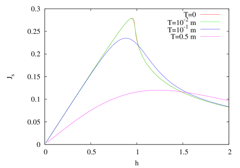
Figure 2: The current versus flux curves for $\Delta=0.2m$ at varying temperature. For temperatures small ($T=0.01m$) compared with $\Delta,m$ the curve is indistinguishable from the zero temperature curve. As temperature become comparable with $\Delta$ the maximum of the current becomes broader and shifts to higher flux. For temperature comparable with $m$, the maximum becomes very broad.

If we turn to the current susceptibility, which has a logarithmic divergence at the critical flux in the ground state, its positive temperature expression is:

$$\frac{\partial^{2}f}{\partial^{2}h}= \frac{1}{\pi u}-\sum_{r=\pm}\int_{0}^{+\infty}\frac{dk}{2\pi}\left[\frac{\partial^{2}E_{r}(k)}{\partial h^{2}}\tanh\left(\frac{E_{r}(k)}{2k_{B}T}\right)+\right.$$ (46)

$$\left.\left(\frac{\partial E_{r}(k)}{\partial h}\right)^{2}\frac{1}{2k_{B}T\cosh^{2}\left(\frac{E_{r}(k)}{2k_{B}T}\right)}\right],$$

Exactly at the critical point $h=\sqrt{m^{2}-\Delta^{2}}$, we find that:

$$\frac{\partial^{2}E_{-}(k)}{\partial h^{2}}=\frac{h^{2}}{2m\Delta u|k|}+O(|k|),$$ (47)

so that $\frac{\partial J}{\partial h}\sim\frac{h^{2}}{4\pi m\Delta u}\ln(1/T)$. In the general case, the divergence of $\partial_{h}J$ is controlled by the integral:

$$\int_{0}^{\Lambda}\frac{dk}{E_{-}(k)}\tanh\left(\frac{E_{-}(k)}{2k_{B}T}\right).$$ (48)

If we take $T=0$, the integral will have a logarithmic divergence in the limit of $h\to\sqrt{m^{2}-\Delta^{2}}$, indicating the Ising transition. However, for any finite $T$, the hyperbolic tangent will cutoff the divergence for $E_{-}(k)\ll k_{B}T$, and give instead a maximum scaling as $\sim\ln(1/T)$. Therefore, one expects that $\partial_{h}J\sim-\ln[(m-\sqrt{h^{2}+\Delta^{2}})^{2}+(k_{B}T)^{2}]$. Thus, for very low temperature, the slope of the curve $J$ versus $h$ presents a maximum at $h=\sqrt{m^{2}-\Delta^{2}}$ indicating the presence of an inflection point instead of the vertical tangent obtained at $T=0$. If we turn to correlation functions, since our system is one dimensional, at any nonzero temperature its correlation functions always decay exponentially.Landau and Lifshitz (1986) However, in the quantum Ising chain, the correlation length of operators that are long range ordered at zero temperature has been foundSachdev (1996); Sachdev and Young (1997) to behave as $\sim u_{s}(TM)^{-1/2}e^{M/T}$ where $M$ is the gap at zero temperature. By contrast, operators with short-range ordered correlations in the ground state still have a correlation length $\sim u_{s}/M$. The difference between the two classes of operators thus remain distinguishable until $T\sim M$. Therefore, in the “renormalized classical” region, the zero temperature power law peaks in $n_{\sigma}(k\to 0)$ turns into a narrow Lorentzian maximum, while the Lorentzian maximas in $S^{c/s}(k)$ and $C(k)$ remain broad. The distinction between CDW and Meissner phase is lost only at a temperature $k_{B}T\sim E_{-}(0)$.

IV Second incommensuration with repulsive interaction

In previous investigationsDi Dio et al. (2015); Orignac et al. (2016) a second incommensuration (2IC) was obtained when the flux $\lambda=\pi n$ for a two-leg ladder of hard core bosons. The 2IC can be associated to the interchain hopping and manifests in the periodic oscillations of the correlation functions at wavevectors formed by a linear combinations of $\lambda$ and $\Omega$. A very simple picture of the second incommensuration can be obtained in the limit $U_{\perp}\gg t$ where one can use a Jordan-Wigner representation for the bosons.
Using a gauge transformation, the Hamiltonian (II) can be rewritten:

$$H = -t\sum_{j,\sigma}(b^{\dagger}_{j+1,\sigma}b_{j,\sigma}+b^{\dagger}_{j,\sigma}b_{j+1,\sigma})+U\sum_{j}n_{j\uparrow}n_{j\downarrow}$$ (49)

$$+\frac{\Omega}{2}\sum_{j}(e^{i\lambda j}b^{\dagger}_{j,\uparrow}b_{j,\downarrow}+e^{-i\lambda j}b^{\dagger}_{j,\downarrow}b_{j,\uparrow}).$$

In terms of the Jordan-Wigner fermions (62) the interchain hopping has, in general, a complicated non-local expressions:

$$b^{\dagger}_{j,\uparrow}b_{j,\downarrow}=c^{\dagger}_{j,\uparrow}\eta_{j\uparrow}\eta_{j\downarrow}c^{\dagger}_{j,\downarrow}e^{i\pi\sum_{k<j}(n_{k\uparrow}+n_{k\downarrow})},$$ (50)

However, at half-filling, the charge is gapped so that one can approximate,

$$e^{i\pi\sum_{k<j}(n_{k\uparrow}+n_{k\downarrow})}\simeq(-)^{j},$$ (51)

and the remaining gapless spin mode described by an effective spin chain model:

$$H=\frac{4t^{2}}{U}\sum_{n}\vec{S}_{n}\cdot\vec{S}_{n+1}.$$ (52)

The antihermitian operator $\eta_{j\uparrow}\eta_{j\downarrow}$ commutes with the Hamiltonian, and can be replaced by one of its eigenvalues $\pm i$. Then, the interchain hopping reduces to:

$$\frac{\Omega}{2}\sum_{j}(e^{i(\lambda-\pi)j}ic^{\dagger}_{j_{\uparrow}}c_{j_{\downarrow}}+H.c.),$$ (53)

and, having in mind the Jordan-Wigner transformation (62), it reduces to $\Omega\sum_{j}S_{j}^{y}$ when $\lambda=\pi$. Therefore, it acts on the spin chain (52) as a uniform magnetic field, and induces a magnetization along the $y$ axis. Such magnetization also gives rise to incommensurationGiamarchi (2004) in the correlation functions of the spin components $x$ and $z$. This treatment represents the simplest way to understand the origin of a second-incommensuration in the correlation functions. However, in the case away from half-filling, the second incommensuration could not be deduced as straightforwardlyOrignac et al. (2016) and one had to resort to a modified mean-field theory.
Here, we want to present another approach, using a canonical transformation that avoids some of the shortcomings of the mean-field theory. If we bosonize the Jordan-Wigner fermionic version of the Hamiltonian (49) we obtain:

$$H=\sum_{\nu=c,s}\int\frac{dx}{2\pi}\left[u_{\nu}K_{\nu}(\pi\Pi_{\nu})^{2}+\frac{u_{\nu}}{K_{\nu}}(\partial_{x}\phi_{\nu})^{2}\right]$$

$$+\frac{\Omega}{2\pi a}\int dx\left[e^{i\sqrt{2}\phi_{c}}(e^{-i\sqrt{2}(\theta_{s}+\phi_{s})}+e^{-i\sqrt{2}(\theta_{s}-\phi_{s})})+\mathrm{H.c.}\right]$$

$$-\frac{2g_{1\perp}}{(2\pi a)^{2}}\int dx\cos\sqrt{8}\phi_{s}.$$ (54)

Then we consider the action of the unitary operator:

$$U=\exp\left[-i\int\frac{dx}{\pi}\phi_{c}(x)\partial_{x}\phi_{s}\right]$$ (55)

Such canonical transformation gives a controlled approximation in the limit of $K_{c}\to 0$. Indeed, by rescaling $\phi_{c}\to\sqrt{K_{c}}\phi_{c}$, $\theta_{c}\to\theta_{c}/\sqrt{K_{c}}$, the unitary transformation (55) becomes close to identity as $K_{c}\ll 1$ and the resulting perturbations in the transformed Hamiltonian are then small. The transformed Hamiltonian is:

$$U^{\dagger}HU = \int\frac{dx}{2\pi}\left[u_{c}K_{c}(\pi\Pi_{c})^{2}+u_{s}K_{s}(\pi\Pi_{s})^{2}\right.$$ (56)

$$+ \left.\left(u_{s}K_{s}+\frac{u_{c}}{K_{c}}\right)(\partial_{x}\phi_{c})^{2}+\left(u_{c}K_{c}+\frac{u_{s}}{K_{s}}\right)(\partial_{x}\phi_{s})^{2}\right]$$

$$+\int dx(u_{s}K_{s}\Pi_{s}\partial_{x}\phi_{c}-u_{c}K_{c}\Pi_{c}\partial_{x}\phi_{s})$$

$$+\frac{\Omega}{2\pi a}\int dx\cos\sqrt{2}\theta_{s}\cos\sqrt{2}\phi_{s}$$

$$-\frac{2g_{1\perp}}{(2\pi a)^{2}}\int dx\cos\sqrt{8}\phi_{s}$$

Neglecting the spin-charge interaction from the third line of the Hamiltonian, one finds the Hamiltonian of an XXZ spin chain in a uniform transverse field.Giamarchi and Schulz (1988); Nersesyan et al. (1993) Using a rotation (see App. C) one can find the ground state of that HamiltonianGiamarchi and Schulz (1988); Nersesyan et al. (1993) and obtain its correlation functions. In the gapless phase, one finds:

$$\langle\rho(j)\rho(j^{\prime})\rangle\sim\langle\sigma^{z}(j)\sigma^{z}(j^{\prime})\rangle\sim\frac{(-1)^{j-j^{\prime}}}{|j-j^{\prime}|}$$ (58)

$$+ \frac{1}{2\pi^{2}(j-j^{\prime})^{2}}\cos\left(\frac{h_{s}(j-j^{\prime})}{u_{s}}\pm\lambda(j-j^{\prime})\right)$$

$$\langle j_{\perp}(j)j_{\perp}(j^{\prime})\rangle\sim\frac{(-1)^{j-j^{\prime}}}{|j-j^{\prime}|}$$

$$+\frac{1}{2\pi^{2}(j-j^{\prime})^{2}}\cos\left(\frac{h_{s}(j-j^{\prime})}{u_{s}}\pm\lambda(j-j^{\prime})\right),$$

with $h_{s}=O(\Omega)$. The correlation functions will therefore present periodic oscillations of wavevector formed of linear combinations of $\lambda$ and $h_{s}/u_{s}$ with integer coefficients, i. e. besides the incommensuration resulting from the flux, a second incommensuration resulting from interchain hopping is obtained. At large $\Omega$ a gapped phase can form in which either the spin-spin or the conversion current correlation will show a quasi long range order. In such case, the oscillations associated with the second incommensuration become exponentially damped, but give rise to Lorentzian-like peaks in the structure factors. When $\Omega$ is low, a charge density wave can be stabilized. Such situation is possible in the case of attractive interaction, and making attraction between opposite spins stronger is detrimental to the observation of the second incommensuration. This explains why, in Ref. Orignac et al., 2017, we were not observing a competition of Ising and second incommensuration in the attractive case. At odds, in the repulsive case, the second incommensuration is very robust.

V The Hard-core limit

In this section we report numerical results on the effect of the interaction between opposite spins when the repulsion between bosons of the same spin is infinite (hard-core case). Here we focus on the repulsive case, since results obtained in the attractive case have been discussed in Ref. Orignac et al., 2017, where we found that instead of having a single flux-driven Meissner to Vortex transition, the commensurate Meissner phase and the incommensurate Vortex phase leave space to a Meissner charge-density wave and to a melted vortex phase with short range order. The transition from the Meissner to the charge density wave phase was in the Ising universality class, as predicted by fermionization. With a repulsive interaction we find that the observation of the Ising transition becomes difficult even though signatures of a vortex melting remain visible.

We show results from DMRG simulations for the filling $\rho=0.5$ per rung. We fix interchain hopping $\Omega/t$ and consider different values of the applied flux $\lambda$ with varying the interaction strength $U_{\perp}$. Simulations are performed in Periodic Boundary Conditions (PBC) for $L=32$ and up to $L=64$ in some selected cases, keeping up to $M=841$ states during the renormalization procedure. The truncation error, that is the weight of the discarded states, is at most of order $10^{-5}$, while the error on the ground-state energy is of order $10^{-4}$ at most.

At variance with attractive case, for filling different from unity, in the absence of an applied field we do not expect the transition from the superfluid Meissner phase to the density wave phaseHu et al. (2009) since repulsion only gives rise to a marginally irrelevant perturbation. Thus, the phase diagram in the presence of flux is expected to be qualitatively different from the one with attraction.

In Fig. 3 we show the response functions, $S^{c}(k)$ for the attractive case and $S^{s}(k)$ for the repulsive case, as they evolve upon increasing the strength of interchain interaction, when $\lambda=0$. As already discussed in Sec. II.1,in the hard-core case, attractive interchain interaction is expected to give rise to charge density wave, while in the repulsive case there is not a spin density wave.

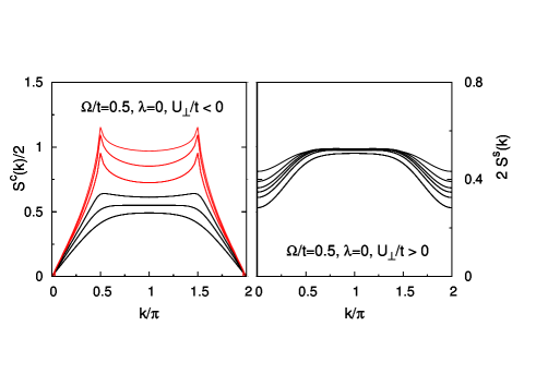
Figure 3: Left panel: $S^{c}(k)$ for the attractive case. Right panel: $S^{s}(k)$ for the repulsive case. Interaction strength is $|U_{\perp}|/t=\pm 1.0,1.5,2.0,3.0$ and $6.0$ from bottom to top curves. Solid black curves indicate a Meissner state, while red solid curves indicate a CDW where the peaks at $k=2k_{F}$ develop. Data from $L=64$ DMRG simulations in PBC at $\lambda=0$ for $\rho=0.5$, at $\Omega/t=0.5$. Color online.

In the left panel of Fig. 3, peaks in $S^{c}(k)$ ($U_{\perp}/t<0$) develop at $k=\pi/2$ and $k=3\pi/2$ as attraction increases and the system enters the in-phase density wave phase. Meanwhile in the right panel of Fig. 3, $S^{s}(k)$ ($U_{\perp}/t>0$) never develops peaks and in fact becomes almost flat as the bosons become more localized, as repulsion is increased. Hence, as expected from marginal irrelevance of interchain repulsion, the spin density wave phase is unfavored.

In order to detect the density wave phases we choose a value of $\Omega/t$ sufficiently large and an applied flux close to the value at which the commensurate-incommensurate transition between the Meissner and the Vortex phases occurs in the absence of interchain interaction. Let us note that the Luttinger parameters $K_{c}$ and $K_{s}$ have a different dependence on the interchain interaction. In the attractive case $K_{c}$ is enhanced and $K_{s}$ is reduced, thus the region of stability of the Meissner phase is reduced and the system is more prone to reach the in-phase density wave and vortex regime. On the contrary, in the repulsive case $K_{c}$ is reduced and $K_{s}$ is increased and, as a consequence, the Meissner phase becomes more stable at the expense of the Vortex and density wave ones.

We consider the following case: $\Omega/t=0.125$ at different applied fluxes. At $\lambda\lesssim\lambda_{c}(U_{\perp}=0)$, .i.e just before the C-IC transition occurs, the system never develops a density wave. In Fig. 4 we show the behavior of the spin and the charge response functions $S^{s}(k)$ and $S^{c}(k)$ respectively, for small and large interaction interaction strength. On increasing the strength the spin static structure factor develops shoulders at $k=2k_{F}=\pm\pi/2$ signaling the incipient transition towards a density wave phase, while the static structure factor for low momentum show the expected linear behavior $S^{c}(k)\simeq\frac{2K_{c}}{\pi}|k|$ for gapless charge excitations. $K_{c}$ smoothly decreases as a function of $U_{\perp}$, going from one, as for a non-interacting hard-core Bose system, towards $1/2$ as shown from the slope of the low momentum linear behavior of $S^{c}(k)$ (see Fig. 4).

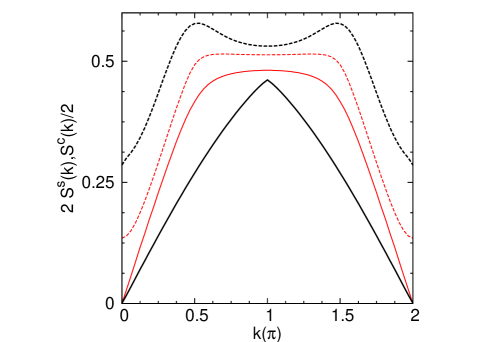
Figure 4: $S^{c}(k)$and $S^{s}(k)$ for the repulsive case, respectively solid and dotted lines, for $U_{\perp}/t=0.5$ and $5.5$, red and black curves respectively. Data from $L=64$ DMRG simulations in PBC at $\lambda=0.0625\pi$, for $\Omega/t=0.125$ and $\rho=0.5$. Color online.

The asymmetry between the attractive and the repulsive case persists in the presence of an applied flux, as shown in Fig. 5, where we follow the response functions change when we increase the interaction strength at fixed $\lambda$ and $\Omega/t=0.5$. At small $|U_{\perp}|$, panel $(c)$ and $(b)$ we start from Meissner phase where the momentum distribution has a single peak at $k=0$, but for larger interaction strength, while in the attractive case we are in a melted Vortex phase, panel $(a)$, in the repulsive case the system is still in the Meissner phase and $S^{s}(k)$ shows only shoulders at $k=2k_{F}$ (panel $(d)$).

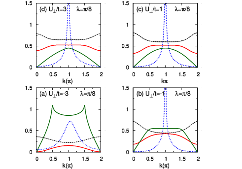
Figure 5: $S^{c}(k)$ and $S^{s}(k)$ are respectively shown as dark-green and red solid lines in all panels. Blue dotted lines are for spin resolved momentum distribution $n_{\sigma}(k)$ whose argument has been shifted shifted of $\pi$ and black dashed lines are for rung-rung correlation function $C(k)$. Panels $a,b,c$ and $d$ are respectively for $U_{\perp}=-3,-1,1$ and $3$. Data from $L=64$ DMRG simulations in PBC at $\lambda=\pi/8$, for $\Omega/t=0.5$ and $\rho=0.5$. Color online.

In the following we investigate the system for fixed $\Omega/t=0.125$ and at a fixed applied flux for which the system is in the Vortex state in the absence of interaction between the chains ($U_{\perp}=0$).

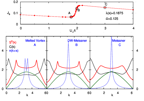
Figure 6: Upper panel shows the spin current $J_{s}$ as a function of strength of interchain interaction, solid red line is only a guide to eye. Panels below show $8S^{s}(k)$ (red solid line), $4C(k)$ (black dashed line), and $n(k)$ (blue dotted line) where the argument of this last quantity has been shifted of $\pi$. Left, center and right panel shows these quantities for the cases indicated by the point A, B and C in the upper panel, respectively corresponding to cases where the system is in the melted Vortex phase, in the CDW–Meissner phase and in the Meissner phase. Data shown are from DMRG simulations in PBC for L=32. Color online.

In the absence of the interaction the spin response function $S^{s}(k)$ displays the expected linear behavior at small momentum and a discontinuity in the derivative at $k=2k_{F}$ Orignac et al. (2016). As we increase the interaction strength (panel A in Fig. 6) the spin structure factor develops peaks at $k=\pi/2$ and $k=3\pi/2$ and an almost quadratic behavior at small wavevector. The quadratic behavior indicates that spin excitations remain gapped, while the presence of peaks at $k=\pi/2,3\pi/2$ is the signature of a zig-zag charge density wave (in the ladder language) or a spin density wave (in the spin-orbit language). The momentum distribution as well the rung-rung response function $C(k)$ develop two separate peaks indicating the presence of an incommensuration. Thus, we can identify the phase to the so-called melted Vortex phase.Orignac et al. (2017) For large value of interaction, panel $C$ of Fig. 6, the system is in strongly correlated Meissner phase, indeed momentum distribution show only one peak centered around $k=0$, and $S^{s}(k)$ shows the incipient transition towards the CDW-Meissner phase in its spin response. In panel B, we have an intermediate situation, where the DW peaks are still visible in the spin response function, but not incommensuration. We conjecture that this corresponds to the so-called charge-density Meissner phase.

In the upper panel of Fig. 6 we show the spin current $J_{s}$ as a function of the strength of interchain interaction when the system goes from the Vortex state to the Meissner one: there is no cusp indicating a square root threshold singularity typical of the C-IC transition, instead the spin current only shows at most a vertical tangent indicating a possible logarithmic divergence of its derivative. To summarize, under application of interleg repulsion, the Vortex phase becomes first a melted vortex phase via a BKT transition, then past the disorder point a DW-Meissner is formed, and finally the Meissner state is stabilized at large repulsion.

As discussed in the previous section, in the presence of the so-called second incommensuration,Di Dio et al. (2015); Orignac et al. (2016) the picture becomes more complicated. Indeed, in such a case, nearby $\lambda\simeq\pi n$ there is a new incommensurate wavevector which gives, in the various structure factors, extra peaks whose magnitude of which is controlled by $\Omega$. In order to illustrate that situation we have made simulations for a larger interchain hopping, namely $\Omega/t=0.5$, so that we have the C-CI transition nearby $\lambda=n\pi$ in absence of interchain interaction and therefore near the occurrence of the second incommensuration.

In Fig. 7 situation at fixed $U_{\perp}/t=1.5$ and $\Omega/t=0.5$ is shown. In the upper panel we follow the spin current as a function of the applied field. It shows the typical behavior of the Meissner phase when it increases as a function of $\lambda$, then it rapidly decreases when entering the Vortex phase which is however short-ranged ordered and finally for larger $\lambda$ enter the quasi long range ordered Vortex phase, as it can also seen from the typical finite size induced oscillations in this quantity.Di Dio et al. (2015) The Meissner phase is shown in panel $A$, while the melted-Vortex phase is shown in panel $B$, where the spin response function has the expected peaks at $k=\pi/2$ and $3\pi/2$, yet it has the low momentum behavior observed in the presence of a second incommensuration.Orignac et al. (2016) In this case, in the momentum distribution is possible to see besides the primary peaks also the secondary peaks related to the second incommensuration. These peaks can be seen also in the rung-rung correlation function $C(k)$. However, both of these functions do not show appreciable size effects attesting the short range of the incommensurate order. In panel $C$ we recover the quasi-long range ordered Vortex phase.

As a last comment we want to stress the fact that in the rung-rung current correlation function in the Meissner phase, see panel $C$ of Fig. 6 and panel $A$ of Fig. 7, shows respectively a Lorentzian-like peak and a cusp centered at $k=4k_{F}=\pi$ as the result of higher order term in the Haldane expansion when we derive the rung current. This cusp is present since the exponent $K_{c}$ is decreasing with repulsion, thus enhancing the contribution of the contribution at $\pi$ compared with the attractive case.

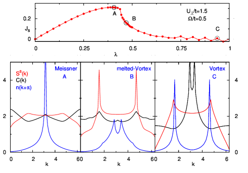
Figure 7: Upper panel shows the spin current $J_{s}$ as a function of the applied flux, red line is only a guide to eye. Panels below show $S^{s}(k)$ (red solid line), $C(k)$ (black line), $n_{\sigma}(k)$ (blue line) where the argument of this last quantity has been shifted of $\pi$. Left, center and right panels show these quantities for the cases indicated by the point $A$, $B$ and $C$ in the upper panel, respectively corresponding to cases where the system is in the Meissner phase, in the melted-Vortex phase and in the Vortex phase. Data shown are from DMRG simulations in PBC for L=64. Color online.

VI Conclusions

To conclude, we have analyzed the phase diagram of boson ladder in the presence of an artificial gauge field, when a repulsive interchain interaction is switched on. We have shown, using bosonization, fermionization and DMRG approach, that the the commensurate-incommensurate transition between the Meissner phase and the QLRO vortex phase is replaced by an Ising-like transition towards a commensurate zig-zag density wave phase. The fermionization approach has allowed us to predict the existence of a disorder point after which the bosonic Green’s functions and the rung current correlation function develop exponentially damped oscillations in real space while zig-zag density wave phase persists. This phase is recognized as a melted vortex phase. Differently from the attractive interaction, a second-incommensuration, i.e. an extra periodic oscillation of the correlation functions at wavevectors formed by a linear combinations of the flux and the interchain interaction, dominates even away from half-filling. As numerically shown, the hard core limit in the chains favors the zig-zag density wave phase. Our predictions on the melting of vortices in Bose-Einstein condensates and on the second incommensuration in optical lattices can be traced in current experiments by the measuring the static structure factors and momentum distributions, together with the rung current.

VII Acknowledgments

We acknowledge A. Celi, M. Calvanese Strinati and E. Tirrito for fruitful discussions. Simulations were performed at Università di Salerno, Università di Trieste and Democritos local computing facilities. M. Di Dio and S. De Palo thank F. Ortolani for the DMRG code. E. Orignac acknowledges hospitality from Università of Salerno.

Appendix A Hard core boson limit and mappings

That limit corresponds to $U_{\uparrow\uparrow}=U_{\downarrow\downarrow}\to+\infty$. In that limit, the bosonic ladder can be mapped to an anisotropic two-leg ladder model with Dzyaloshinskii-MoriyaDzyaloshinskii (1958); Moriya (1960) interaction, and to the Hubbard model.

A.1 Mapping to a spin ladder

If we consider hard core bosons, we can use the mapping of hard core bosons to spins 1/2:

$$b_{j}^{\dagger}=S_{j}^{+}$$ (59)

$$b_{j}=S_{j}^{-}$$ (60)

$$b^{\dagger}_{j}b_{j}=S_{j}^{z}+\frac{1}{2},$$ (61)

which can be deduced easily from the Holstein-Primakoff representationHolstein and Primakoff (1940) of spin-1/2 operators. With such mapping, we can rewrite the Hamiltonian (II) as a two-leg ladder Hamiltonian in which the upper and the lower leg have uniform Dzyaloshinskii Moriya interaction. In the two leg ladder representation, $\Omega$ and $U_{\uparrow\downarrow}$ become the rung exchange interaction, $t\cos(\lambda/2)$ and $U_{\uparrow\uparrow},U_{\uparrow\uparrow}$ become the leg exchange interaction, $t\sin(\lambda/2)$ becomes the Dzyaloshinskii-Moriya term.

A.2 Mapping to spin-1/2 fermions

Another possible mapping in the case of hard core bosons $U_{\uparrow\uparrow},U_{\downarrow\downarrow}\to\infty$ is to the Hubbard model. This mapping is only valid when $\Omega=0$, but it allows to take advantage of the integrability of the Hubbard model.Lieb and Wu (1968); Frahm and Korepin (1990, 1991); Andrei (1993) The mapping, is obtained from the Jordan-Wigner transformationJordan and Wigner (1928) that maps hard core bosons operators $b_{j\sigma}$ to fermion operators $c_{j\sigma}$ :

$$b_{j\sigma} = \eta_{\sigma}c_{j,\sigma}e^{i\pi\sum_{k<j}c^{\dagger}_{k,\sigma}c_{k,\sigma}},$$ (62)

$$b^{\dagger}_{j\sigma}b_{j\sigma} = c^{\dagger}_{j,\sigma}c_{j,\sigma},$$ (63)

where $\{\eta_{\sigma},\eta_{\sigma^{\prime}}\}_{+}=\delta_{\sigma\sigma^{\prime}}$. The Hamiltonian (II) with $\Omega=0$ is rewritten as:

$$H=-t\sum_{j,\sigma}(c^{\dagger}_{j+1,\sigma}e^{-i\lambda\sigma}c_{j,\sigma}+\mathrm{H.c.})+U\sum_{j}n_{j,\uparrow}n_{j,\downarrow}$$ (64)

The gauge transformationZvyagin (2012) $c_{j,\sigma}=e^{-i\lambda\sigma j}a_{j,\sigma}$ reduces the Hamiltonian (64) to the Hubbard form. The Hubbard model presents a spin-charge separation. When interactions are repulsive, and away from half-filling, charge and spin modes are gapless, whereas with attractive interactions charge modes are always gapless but spin modes are gapped. In terms of the original bosons, total density modes are always gapless away from half-filling, but the chain antisymmetric density fluctuations are gapped with attractive interaction giving rise to a symmetric density wave phase, gapless with repulsive interaction.

Appendix B Asymptotic behavior of the Green’s functions

To estimate the asymptotic behavior of the Green’s functions, we apply a contour integral methodM.Bender and Orszag (1978) to the integral

$$\bar{I}_{1}(x)=\int_{-\infty}^{\infty}\frac{dk}{2\pi}\frac{e^{ik|x|}}{E_{-}(k)}.$$ (65)

The function $E_{-}(k)$ has only branch cut singularities in the upper half plane. The branch cuts arise either from $h^{2}(uk)^{2}+h^{2}m^{2}+m^{2}\Delta^{2}<0$ or $(uk)^{2}+m^{2}+\Delta^{2}+h^{2}-2\sqrt{h^{2}(uk)^{2}+h^{2}m^{2}+m^{2}\Delta^{2}}<0$. The first branch cut, obtained for $u^{2}k^{2}<-m^{2}(1+\Delta^{2}/h^{2})$ gives a contribution decaying as $e^{-m\sqrt{1+\Delta^{2}/h^{2}}|x|/u}$, that can be ignored for $|x|\gg m/u$. The contribution of the cuts of the second type depends whether $h<m$ or $h>m$. For $h<m$, there is a single branch cut extending along the imaginary axis from $i|\Delta-\sqrt{m^{2}-h^{2}}|/u<k<i(\Delta+\sqrt{m^{2}-h^{2}})$. We can rewrite the integral (65) as:

$$\bar{I}_{1}(x)=\int_{\frac{|\Delta-\sqrt{m^{2}-h^{2}}|}{u}}^{\frac{\Delta+\sqrt{m^{2}-h^{2}}}{u}}\frac{dk}{\pi}\frac{e^{-k|x|}}{E_{-}(ik)}.$$ (66)

showing that $I_{1}(x)\sim e^{-\frac{|\Delta-\sqrt{m^{2}-h^{2}}||x|}{u}}$. This gives a correlation length diverging as $\sim|m-\sqrt{h^{2}+\Delta^{2}}|^{-1}$ near the Ising transition.

For $h>m$, there are two branch cuts given by:

$$\sqrt{(uk)^{2}+m^{2}+\frac{m^{2}\Delta^{2}}{h^{2}}}=h\pm i\Delta\sqrt{1-\frac{m^{2}}{h^{2}}}\cosh\alpha,$$ (67)

and $\alpha$ real. The integration path in the complex plane is represented on Fig. 8. The branch cuts terminate at the branch points $k_{d}^{(\pm)}=i\frac{\Delta}{u}\pm\frac{\sqrt{h^{2}-m^{2}}}{u}$ such that $E_{-}(k_{d}^{(\pm)})^{2}=0$. The long distance behavior of $\bar{I}_{1}$ is determined by these two branch points as:

$$\bar{I}_{1}(x)\sim e^{-\frac{\Delta|x|}{u}}\left[e^{i\frac{\sqrt{h^{2}-m^{2}}|x|}{u}}\varphi_{1}(x)+e^{-i\frac{\sqrt{h^{2}-m^{2}}|x|}{u}}\varphi_{1}(x)^{*}\right],$$ (68)

so that oscillations of wavevector $\sqrt{h^{2}-m^{2}}/u$ appear in the real space correlation functions for $h>m$. The point $h=m$ is called a disorder pointStephenson (1970a, b). Disorder points are known to occur in frustrated quantum Ising chains in transverse field,Beccaria et al. (2006) bilinear-biquadratic spin-1 chains,Golinelli et al. (1998); Schollwöck et al. (1996) frustrated spin-1/2 Bursill et al. (1995); Deschner and Sørensen (2013) and spin-1 Pixley et al. (2014); Chepiga et al. (2016) chains. They can be classifiedStephenson (1970b) into disorder points of the first kind (with parameter dependent incommensuration) and disorder point of the second kind (with parameter independent incommensuration). In our model, the disorder point is of the first kind.

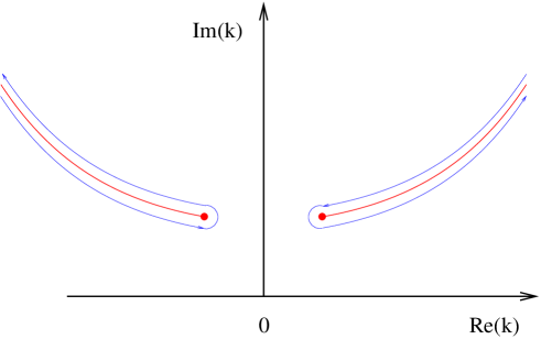
Figure 8: The integration path in complex $k$ plane for $h>m$. The red curves are such that $E_{-}(k)^{2}<0$. The red dots at extremities of the curve are the points where $E_{-}(k)=0$.

Appendix C Second incommensuration and canonical transformation

In this section, we give some details on the rotationGiamarchi and Schulz (1988); Nersesyan et al. (1993) used to diagonalize the Hamiltonian obtained after the unitary transformation of Eq. (55). First, we rewrite our Hamiltonian (56) using nonabelian bosonization:Witten (1984)

$$H_{s}=\frac{2\pi v}{3}\int dx(\vec{J}_{R}\cdot\vec{J}_{R}+\vec{J}_{L}\cdot\vec{J}_{L})+g_{1\parallel}\int dxJ_{R}^{z}J_{L}^{z}$$ (69)

$$+g_{1\perp}\int dx(J_{R}^{x}J_{L}^{x}+J_{R}^{y}J_{L}^{y})+\Omega\int dx(J_{R}^{y}+J_{L}^{y})$$ (70)

with $g_{1\parallel}\neq g_{1\perp}$ . Using a $\frac{\pi}{2}$ rotation around the $y$ axisDi Dio et al. (2015) we can rewrite:

$$H_{s}=\frac{2\pi v}{3}\int dx(\vec{\tilde{J}}_{R}\cdot\vec{\tilde{J}}_{R}+\vec{\tilde{J}}_{L}\cdot\vec{\tilde{J}}_{L})+g_{1\parallel}\int dx\tilde{J}_{R}^{y}\tilde{J}_{L}^{y}$$

$$+g_{1\perp}\int dx(\tilde{J}_{R}^{x}\tilde{J}_{L}^{x}+\tilde{J}_{R}^{z}\tilde{J}_{L}^{z})+\Omega\int dx(\tilde{J}_{R}^{z}+\tilde{J}_{L}^{z})$$ (71)

Finally, returning to abelian bosonization, we obtainGiamarchi and Schulz (1988); Nersesyan et al. (1993)

$$H_{s} = \int\frac{dx}{2\pi}\left[uK(\pi\tilde{\Pi}_{s})^{2}+\frac{u}{K}(\partial_{x}\tilde{\phi}_{s})^{2}\right]-\frac{\Omega}{\pi\sqrt{2}}\int dx\partial_{x}\tilde{\phi}_{s}$$ (72)

$$+\frac{2(g_{1\perp}+g_{1\parallel})}{(2\pi a)^{2}}\int dx\cos\sqrt{8}\tilde{\phi}_{s}$$

$$+\frac{2(g_{1\perp}-g_{1\parallel})}{(2\pi a)^{2}}\int dx\cos\sqrt{8}\tilde{\theta}_{s}$$

As we can see, either we obtain a fixed point with $\tilde{\theta}_{s}$ long range ordered or a gapless fixed point. In both cases since we may eliminate the $\partial_{x}\tilde{\phi}_{s}$ by a shift of the $\tilde{\phi}_{s}$ field, one has $\langle\tilde{\phi_{s}}\rangle=\frac{h_{s}}{\sqrt{2}u_{s}}x$. When $\tilde{\theta}_{s}$ is gapless, this gives rise to the second incommensuration of Ref. Orignac et al., 2016. To be more precise, if we consider the bosonized expression for the observables:

$$U^{\dagger}\rho(x)U = \rho_{0}-\frac{\sqrt{2}}{\pi}\partial_{x}\phi_{c}+\cos\sqrt{2}(\phi_{c}-2\pi\rho_{0}x)\cos\sqrt{2}\phi_{s}$$ (73)

$$U^{\dagger}\sigma^{z}(x)U = -\frac{\sqrt{2}}{\pi}\partial_{x}\phi_{s}+\cos\sqrt{2}(\phi_{c}-2\pi\rho_{0}x)\sin\sqrt{2}\phi_{s}$$ (74)

$$U^{\dagger}j_{\perp}(x)U = \frac{\Omega}{\pi a}\left[\sum_{r=\pm 1}\sin\sqrt{2}(\theta_{s}+r\phi_{s})\cos\sqrt{2}\phi_{c}\right.$$

$$+ \cos\sqrt{2}(\theta_{s}+r\phi_{s})\sin\sqrt{2}\phi_{c}+\sin\sqrt{2}\theta_{s}\cos(\sqrt{2}\phi_{c}+\lambda x)$$

$$+ \left.\cos\sqrt{2}\theta_{s}\sin(\sqrt{2}\phi_{c}+\lambda x)\right]$$

and perform here the shift of the field $\tilde{\phi}_{s}\rightarrow\phi_{s}-\frac{h_{s}x}{\sqrt{2}u_{s}}x$ and using a rotation of the $SU(2)_{1}$ primary fieldsDi Dio et al. (2015), we reexpress the observables as:

$$U^{\dagger}\rho(x)U = \rho_{0}-\frac{\sqrt{2}}{\pi}\partial_{x}\phi_{c}$$ (75)

$$+\cos\sqrt{2}(\phi_{c}-2\pi\rho_{0}x)\cos\left(\sqrt{2}\tilde{\phi_{s}}+\frac{h_{s}}{u_{s}}x\right)$$

$$U^{\dagger}\sigma^{z}(x)U = -\frac{1}{\pi a}\sum_{r,r^{\prime}=\pm}e^{ir\sqrt{2}(\tilde{\theta}_{s}+r^{\prime}\tilde{\phi}_{s})+irr^{\prime}\frac{h_{s}x}{u_{s}}}$$ (76)

$$-\cos\sqrt{2}(\phi_{c}-2\pi\rho_{0}x)\cos\sqrt{2}\tilde{\theta}_{s}$$

$$U^{\dagger}j_{\perp}(x)U = \frac{\Omega}{\pi a}\left[\sum_{r=\pm 1}\sin\sqrt{2}\left(\tilde{\theta}_{s}+r\tilde{\phi}_{s}+\frac{h_{s}}{u_{s}}x\right)\cos\sqrt{2}\phi_{c}\right.$$

$$-\frac{1}{\pi\sqrt{2}} \partial_{x}\tilde{\phi_{s}}\sin\sqrt{2}\phi_{c}+\sin\sqrt{2}\tilde{\theta}_{s}\cos(\sqrt{2}\phi_{c}+\lambda x)$$ (77)

$$+\left.\sin\left(\sqrt{2}\tilde{\phi}_{s}+\frac{h_{s}}{u_{s}}x\right)\sin(\sqrt{2}\phi_{c}+\lambda x)\right]$$

In the gapless case, taking the expectation value gives the second incommensuration.

References

- Jaksch and Zoller (2005) D. Jaksch and P. Zoller, Ann. Phys. (N. Y.) 315, 52 (2005), cond-mat/0410614.
- Lewenstein et al. (2007) M. Lewenstein, A. Sanpera, V. Ahufinger, B. Damski, A. Sen De, and U. Sen, Ann. Phys. (N. Y.) 56, 243 (2007), cond-mat/0606771.
- Bloch et al. (2008) I. Bloch, J. Dalibard, and W. Zwerger, Rev. Mod. Phys. 80, 885 (2008).
- Cazalilla et al. (2011) M. A. Cazalilla, R. Citro, T. Giamarchi, E. Orignac, and M. Rigol, Rev. Mod. Phys. 83, 1405 (2011).
- Lin et al. (2011) Y. Lin, K. Jimenez-Garcia, and I. B. Spielman, Nature (London) 471, 83 (2011).
- Dalibard et al. (2011) J. Dalibard, F. Gerbier, G. Juzeliūnas, and P. Öhberg, Rev. Mod. Phys. 83, 1523 (2011).
- Galitski and Spielman (2013) V. Galitski and I. B. Spielman, Nature (London) 494, 49 (2013).
- Celi et al. (2014) A. Celi, P. Massignan, J. Ruseckas, N. Goldman, I. B. Spielman, G. Juzeliūnas, and M. Lewenstein, Phys. Rev. Lett. 112, 043001 (2014).
- Livi et al. (2016) L. F. Livi, G. Cappellini, M. Diem, L. Franchi, C. Clivati, M. Frittelli, F. Levi, D. Calonico, J. Catani, M. Inguscio, et al., Phys. Rev. Lett. 117, 220401 (2016).
- Regnault and Jolicoeur (2003) N. Regnault and T. Jolicoeur, Phys. Rev. Lett. 91, 030402 (2003), eprint arXiv:cond-mat/0212477.
- Atala et al. (2014) M. Atala, M. Aidelsburger, M. Lohse, J. Barreiro, B. Paredes, and I. Bloch, Nat. Phys. 10, 588 (2014).
- Kardar (1986) M. Kardar, Phys. Rev. B 33, 3125 (1986).
- Orignac and Giamarchi (2001a) E. Orignac and T. Giamarchi, Phys. Rev. B 64, 144515 (2001a).
- Cha and Shin (2011) M.-C. Cha and J.-G. Shin, Phys. Rev. A 83, 055602 (2011).
- Ambegaokar et al. (1982) V. Ambegaokar, U. Eckern, and G. Schön, Phys. Rev. Lett. 48, 1745 (1982).
- Korshunov (1989) S. E. Korshunov, Europhys. Lett. 9, 107 (1989).
- Roushan et al. (2017) P. Roushan, C. Neill, A. Megrant, Y. Chen, R. Babbush, R. Barends, et al., Nat. Phys. 13, 146 (2017).
- Le Hur et al. (2016) K. Le Hur, L. Henriet, A. Petrescu, K. Plekhanov, G. Roux, and M. Schiró, C. R. Phys. 17, 808 (2016), eprint arXiv:1505.00167.
- Romero et al. (2017) G. Romero, E. Solano, and L. Lamata, in Quantum Simulations with Photons and Polaritons: Merging Quantum Optics with Condensed Matter Physics, edited by D. Angelakis (Springer, Heidelberg, 2017), Quantum Science and Technology Series, chap. 7, p. 153.
- Dhar et al. (2012) A. Dhar, M. Maji, T. Mishra, R. V. Pai, S. Mukerjee, and A. Paramekanti, Phys. Rev. A 85, 041602 (2012).
- Dhar et al. (2013) A. Dhar, T. Mishra, M. Maji, R. V. Pai, S. Mukerjee, and A. Paramekanti, Phys. Rev. B 87, 174501 (2013).
- Petrescu and Le Hur (2013) A. Petrescu and K. Le Hur, Phys. Rev. Lett. 111, 150601 (2013).
- Po et al. (2014) H. C. Po, W. Chen, and Q. Zhou, Phys. Rev. A 90, 011602 (2014).
- Xu et al. (2014) Z. Xu, W. Cole, and S. Zhang, Phys. Rev. A 89, 051604(R) (2014), eprint arXiv:1403.3491.
- Zhao et al. (2014) J. Zhao, S. Hu, J. Chang, F. Zheng, P. Zhang, and X. Wang, Phys. Rev. B 90, 085117 (2014).
- Wei and Mueller (2014) R. Wei and E. J. Mueller, Phys. Rev. A 89, 063617 (2014).
- Hügel and Paredes (2014) D. Hügel and B. Paredes, Phys. Rev. A 89, 023619 (2014).
- Piraud et al. (2014) M. Piraud, Z. Cai, I. P. McCulloch, and U. Schollwöck, Phys. Rev. A 89, 063618 (2014).
- Piraud et al. (2015) M. Piraud, F. Heidrich-Meisner, I. P. McCulloch, S. Greschner, T. Vekua, and U. Schollwöck, Phys. Rev. B 91, 140406 (2015).
- Keleş and Oktel (2015) A. Keleş and M. O. Oktel, Phys. Rev. A 91, 013629 (2015).
- Greschner et al. (2015) S. Greschner, M. Piraud, F. Heidrich-Meisner, I. McCulloch, U. Schollwöck, and T. Vekua, Phys. Rev. Lett. 115, 190402 (2015).
- Greschner et al. (2016) S. Greschner, M. Piraud, F. Heidrich-Meisner, I. P. McCulloch, U. Schollwöck, and T. Vekua, Phys. Rev. A 94, 063628 (2016).
- Petrescu and Le Hur (2015) A. Petrescu and K. Le Hur, Phys. Rev. B 91, 054520 (2015).
- Barbiero et al. (2016) L. Barbiero, M. Abad, and A. Recati, Phys. Rev. A 93, 033645 (2016), eprint arXiv:1403.4185.
- Peotta et al. (2014) S. Peotta, L. Mazza, E. Vicari, M. Polini, R. Fazio, and D. Rossini, J. Stat. Mech.: Theory Exp. 2014, P09005 (2014).
- Di Dio et al. (2015) M. Di Dio, S. De Palo, E. Orignac, R. Citro, and M.-L. Chiofalo, Phys. Rev. B 92, 060506 (2015).
- Orignac et al. (2016) E. Orignac, R. Citro, M. Di Dio, S. De Palo, and M. L. Chiofalo, New J. Phys. 18, 055017 (2016).
- Petrescu et al. (2016) A. Petrescu, M. Piraud, G. Roux, I. McCulloch, and K. L. Hur, Precursor of laughlin state of hard core bosons on a two leg ladder, arXiv:1612.05134 (2016).
- Barbarino et al. (2016) S. Barbarino, L. Taddia, D. Rossini, L. Mazza, and R. Fazio, New J. Phys. 18, 035010 (2016).
- Strinati et al. (2017) M. C. Strinati, E. Cornfeld, D. Rossini, S. Barbarino, M. Dalmonte, R. Fazio, E. Sela, and L. Mazza, Phys. Rev. X 7, 021033 (2017).
- Tokuno and Georges (2014) A. Tokuno and A. Georges, New J. Phys. 16, 073005 (2014).
- Uchino and Tokuno (2015) S. Uchino and A. Tokuno, Phys. Rev. A 92, 013625 (2015).
- Bilitewski and Cooper (2016) T. Bilitewski and N. R. Cooper, Phys. Rev. A 94, 023630 (2016).
- Greschner and Vekua (2017) S. Greschner and T. Vekua, Vortex-hole duality: a unified picture of weak and strong-coupling regimes of bosonic ladders with flux, arXiv:1704.06517 (2017).
- Guo and Poletti (2017) C. Guo and D. Poletti, Dissipatively driven strongly interacting bosons in a gauge field, arXiv preprint arXiv:1705.07633 (2017).
- Richaud and Penna (2017) A. Richaud and V. Penna, Quantum dynamics of bosons in a two-ring ladder: dynamical algebra, vortex-like excitations and currents, arXiv preprint arXiv:1705.02115 (2017).
- Romen and Läuchli (2017) C. Romen and A. M. Läuchli, Chiral Mott insulators in frustrated Bose-Hubbard models on ladders and two-dimensional lattices: a combined perturbative and density matrix renormalization group study (2017), eprint arXiv:1711.01909.
- Laughlin (1983) R. B. Laughlin, Phys. Rev. Lett. 50, 1395 (1983).
- Natu (2015) S. S. Natu, Bosons with long range interactions on two-leg ladders in artificial magnetic fields (2015), arXiv:1506.04346.
- Orignac et al. (2017) E. Orignac, R. Citro, M. Di Dio, and S. De Palo, Phys. Rev. B 96, 014518 (2017), arXiv:1703.07742.
- Bohr et al. (1982) T. Bohr, V. L. Pokrovskiǐ, and A. L. Talapov, JETP Lett. 35, 203 (1982).
- Bohr (1982) T. Bohr, Phys. Rev. B 25, 6981 (1982), [Phys. Rev. B 26, 5257(E) (1982)].
- Haldane et al. (1983) F. D. M. Haldane, P. Bak, and T. Bohr, Phys. Rev. B 28, 2743 (1983).
- Schulz (1983) H.-J. Schulz, Phys. Rev. B 28(5), 2746 (1983).
- Horowitz et al. (1983) B. Horowitz, T. Bohr, J. Kosterlitz, and H. J. Schulz, Phys. Rev. B 28, 6596 (1983).
- Stephenson (1970a) J. Stephenson, Can. J. Phys. 48, 1724 (1970a).
- Stephenson (1970b) J. Stephenson, Phys. Rev. B 1, 4405 (1970b).
- Berezinskii (1971) V. L. Berezinskii, Sov. Phys. JETP 32, 493 (1971).
- Kosterlitz and Thouless (1973) J. M. Kosterlitz and D. J. Thouless, J. Phys. C 6, 1181 (1973).
- Cazalilla and Ho (2003) M. A. Cazalilla and A. F. Ho, Phys. Rev. Lett. 91, 150403 (2003).
- Mathey et al. (2000) L. Mathey, I. Danshita, and C. W. Clark, Phys. Rev. A 79, 011602(R) (2000).
- Hu et al. (2009) A. Hu, L. Mathey, I. Danshita, E. Tiesinga, C. J. Williams, and C. W. Clark, Phys. Rev. A 80, 023619 (2009).
- Haldane (1981) F. D. M. Haldane, Phys. Rev. Lett. 47, 1840 (1981).
- Lukyanov and Terras (2003) S. Lukyanov and V. Terras, Nucl. Phys. B 654, 323 (2003), hep-th/0206093.
- Ovchinnikov (2004) A. A. Ovchinnikov, J. Phys.: Condens. Matter 16, 3147 (2004), eprint arXiv:math-ph/0311050.
- Shashi et al. (2012) A. Shashi, M. Panfil, J.-S. Caux, and A. Imambekov, Phys. Rev. B 85, 155136 (2012).
- Hikihara and Furusaki (2003) T. Hikihara and A. Furusaki, Correlation amplitudes for the spin-1/2 xxz chain in a magnetic field (2003), cond-mat/0310391.
- Bouillot et al. (2011) P. Bouillot, C. Kollath, A. M. L uchli, M. Zvonarev, B. Thielemann, C. R egg, E. Orignac, R. Citro, M. Klanjsek, C. Berthier, et al., Phys. Rev. B 83, 054407 (2011), arXiv:1009.0840.
- Giamarchi (2004) T. Giamarchi, Quantum Physics in One Dimension (Oxford University Press, Oxford, 2004).
- Orignac and Giamarchi (1998) E. Orignac and T. Giamarchi, Phys. Rev. B 57, 11713 (1998), eprint cond-mat/9801048.
- Mathey (2007) L. Mathey, Phys. Rev. B 75, 144510 (2007).
- Mathey and Wang (2007) L. Mathey and D.-W. Wang, Phys. Rev. A 75, 013602 (2007).
- Mathey et al. (2009) L. Mathey, I. Danshita, and C. W. Clark, Phys. Rev. A 79, 011602 (2009).
- José et al. (1977) J. V. José, L. P. Kadanoff, S. Kirkpatrick, and D. R. Nelson, Phys. Rev. B 16, 1217 (1977).
- Lecheminant et al. (2002) P. Lecheminant, A. O. Gogolin, and A. A. Nersesyan, Nucl. Phys. B 639, 502 (2002).
- Japaridze and Nersesyan (1978) G. I. Japaridze and A. A. Nersesyan, JETP Lett. 27, 334 (1978).
- Pokrovsky and Talapov (1979) V. L. Pokrovsky and A. L. Talapov, Phys. Rev. Lett. 42, 65 (1979).
- Schulz (1980) H. J. Schulz, Phys. Rev. B 22, 5274 (1980).
- Chitra and Giamarchi (1997) R. Chitra and T. Giamarchi, Phys. Rev. B 55, 5816 (1997).
- Orignac and Giamarchi (2001b) E. Orignac and T. Giamarchi, Phys. Rev. B 64, 144515 (2001b).
- Tsvelik (1990) A. M. Tsvelik, Phys. Rev. B 42, 10499 (1990).
- Wang (2003) Y.-J. Wang, Field-induced ising criticality and incommensurability in anisotropic spin-1 chains, arXiv preprint cond-mat/0306365 (2003).
- Essler and Affleck (2004) F. H. L. Essler and I. Affleck, J. Stat. Mech.: Theory Exp. p. P12006 (2004).
- Shelton et al. (1996) D. G. Shelton, A. A. Nersesyan, and A. M. Tsvelik, Phys. Rev. B 53, 8521 (1996).
- Nersesyan and Tsvelik (1997) A. Nersesyan and A. M. Tsvelik, Phys. Rev. Lett. 78, 3939 (1997), ibid. , 79, E 1171.
- Citro and Orignac (2002) R. Citro and E. Orignac, Phys. Rev. B 65, 134413 (2002), eprint cond-mat/0106020.
- McCoy (1995) B. M. McCoy, in Statistical Mechanics and Field Theory, edited by V. Bazhanov and C. Burden (World Scientific, Singapore, 1995), p. 26, hep-th/9403084.
- Campostrini et al. (2014) M. Campostrini, A. Pelissetto, and E. Vicari, Phys. Rev. B 89, 094516 (2014).
- Zuber and Itzykson (1977) J. B. Zuber and C. Itzykson, Phys. Rev. D 15, 2875 (1977).
- Schroer and Truong (1978) B. Schroer and T. T. Truong, Nucl. Phys. B 144, 80 (1978).
- Boyanovsky (1989) D. Boyanovsky, Phys. Rev. B 39, 6744 (1989).
- Nersesyan (2001) A. A. Nersesyan, in New theoretical approaches to strongly correlated systems, edited by A. M. Tsvelik (Kluwer Academic Publishers, Dordrecht, Netherlands, 2001), vol. 23 of NATO science series. Series II, Mathematics, physics, and chemistry, chap. 4, p. 89.
- M.Bender and Orszag (1978) C. M.Bender and S. A. Orszag, Advanced mathematical methods for scientists and engineers (McGraw-Hill, NY, 1978).
- Sondhi et al. (1997) L. Sondhi, S. M. Girvin, J. P. Carini, and D. Shahar, Rev. Mod. Phys. 69, 315 (1997).
- Sachdev (2000) S. Sachdev, Quantum Phase Transitions (Cambridge University Press, Cambridge, UK, 2000).
- Landau and Lifshitz (1986) L. D. Landau and I. M. Lifshitz, Statistical Physics. 3rd edition (Pergamon Press, Oxford, 1986).
- Sachdev (1996) S. Sachdev, Nucl. Phys. B 464, 576 (1996).
- Sachdev and Young (1997) S. Sachdev and A. P. Young, Phys. Rev. Lett. 78, 2220 (1997), URL http://link.aps.org/doi/10.1103/PhysRevLett.78.2220.
- Giamarchi and Schulz (1988) T. Giamarchi and H. J. Schulz, J. Phys. (Paris) 49, 819 (1988).
- Nersesyan et al. (1993) A. Nersesyan, A. Luther, and F. Kusmartsev, Phys. Lett. A 176, 363 (1993).
- Di Dio et al. (2015) M. Di Dio, R. Citro, S. De Palo, E. Orignac, and M.-L. Chiofalo, Eur. Phys. J. Spec. Top. 224, 525 (2015).
- Dzyaloshinskii (1958) I. Dzyaloshinskii, J. Phys. Chem. Solids 4, 241 (1958).
- Moriya (1960) T. Moriya, Phys. Rev. 120, 91 (1960).
- Holstein and Primakoff (1940) T. Holstein and H. Primakoff, Phys. Rev. 58, 1098 (1940).
- Lieb and Wu (1968) E. H. Lieb and F. Y. Wu, Phys. Rev. Lett. 20, 1445 (1968).
- Frahm and Korepin (1990) H. Frahm and V. E. Korepin, Phys. Rev. B 42, 10553 (1990).
- Frahm and Korepin (1991) H. Frahm and V. E. Korepin, Phys. Rev. B 43, 5663 (1991).
- Andrei (1993) N. Andrei, in Low-Dimensional Quantum Field Theories For Condensed Matter Physicists, edited by S. Lundqvist, G. Morandi, and L. Yu (World Scientific, Singapore, 1993), and references therein.
- Jordan and Wigner (1928) P. Jordan and E. Wigner, Z. Phys. 47, 631 (1928).
- Zvyagin (2012) A. A. Zvyagin, Phys. Rev. B 86, 085126 (2012).
- Beccaria et al. (2006) M. Beccaria, M. Campostrini, and A. Feo, Phys. Rev. B 73, 052402 (2006).
- Golinelli et al. (1998) O. Golinelli, T. Jolicoeur, and E. Sorensen, Incommensurability in the magnetic excitations of the bilinear-biquadratic spin-1 chain (1998), cond-mat/9812296.
- Schollwöck et al. (1996) U. Schollwöck, T. Jolicoeur, and T. Garel, Phys. Rev. B 53, 3304 (1996).
- Bursill et al. (1995) R. Bursill, G. Gehring, D. Farnell, J. Parkinson, T. Xiang, and C. Zeng, J. Phys.: Condens. Matter 7, 8605 (1995).
- Deschner and Sørensen (2013) A. Deschner and E. S. Sørensen, Phys. Rev. B 87, 094415 (2013).
- Pixley et al. (2014) J. Pixley, A. Shashi, and A. H. Nevidomskyy, Physical Review B 90, 214426 (2014).
- Chepiga et al. (2016) N. Chepiga, I. Affleck, and F. Mila, Phys. Rev. B 94, 205112 (2016).
- Witten (1984) E. Witten, Commun . Math. Phys. 92, 455 (1984).