Median Shapes

Abstract

We introduce and begin to explore the mean and median of finite sets of shapes represented as integral currents. The median can be computed efficiently in practice, and we focus most of our theoretical and computational attention on medians. We consider questions on the existence and regularity of medians. While the median might not exist in all cases, we show that a mass-regularized median is guaranteed to exist. When the input shapes are modeled by integral currents with shared boundaries in codimension $1$, we show that the median is guaranteed to exist, and is contained in the envelope of the input currents. On the other hand, we show that medians can be wild in this setting, and smooth inputs can generate non-smooth medians.

For higher codimensions, we show that books are minimizing for a finite set of $1$-currents in $\mathbb{R}^{3}$ with shared boundaries. As part of this proof, we present a new result in graph theory—that cozy graphs are comfortable—which should be of independent interest. Further, we show that regular points on the median have book-like tangent cones in this case.

From the point of view of computation, we study the median shape in the settings of a finite simplicial complex. When the input shapes are represented by chains of the simplicial complex, we show that the problem of finding the median shape can be formulated as an integer linear program. This optimization problem can be solved as a linear program in practice, thus allowing one to compute median shapes efficiently.

We provide open source code implementing our methods, which could also be used by anyone to experiment with ideas of their own. The software could be accessed at https://github.com/tbtraltaa/medianshape.

1 Introduction

Our goal is to study shapes and statistics in shape spaces. The results of any such study depend critically on how we represent shapes, and on what distance we use in that representational space. Given that statistics in shape spaces is not a new endeavor, there have been a variety of choices for both representations of as well as distances between shapes, leading to an equally diverse set of results. For instance, see [5, 11, 14, 30, 31, 37, 39, 48, 49], as well as the references they contain.

In this paper, we take the (mostly) new approach of representing shapes as currents. This approach leads very naturally to the use of flat norm as a distance between shapes. Previous work on related approaches include [3, 4, 46, 54], earlier work by Glaunes and collaborators who used currents to represent 2-dimensional surfaces in $\mathbb{R}^{3}$ and a distance similar to the flat norm [28, 29, 53], as well as the more recent work from the same group by Charon et al. [8, 9, 10] and Kaltenmark [36]. Perhaps the closest previous results to our work is the paper by Berkels, Linkmann, and Rumpf [6].

We work with variational definitions of means and medians, which naturally lead to optimization problems that are easy to state. On the theoretical side, we prove several results on existence and regularity of medians. On the computational side, the optimization problem to find the median turns out to be quite tractable (solvable as a linear program in practice). In fact, the computational tractability also motivated in part our efforts toward the theoretical characterization of the median (as opposed to the mean). We begin by recalling some facts about means and medians.

1.1 Means and Medians in $\mathbb{R}^{d}$

While the mean in the context of a set of numbers $\{x_{i}\}_{i=1}^{N}\subset\mathbb{R}$ or, more generally, a set of points in $\mathbb{R}^{d}$, $\{\mathbf{x}_{i}\}_{i=1}^{N}\subset\mathbb{R}^{d}$, is most often thought of as

$$\bar{\mathbf{x}}=\frac{1}{N}\sum_{i=1}^{N}\mathbf{x}_{i}\,,$$

the variational definition:

$$\bar{\mathbf{x}}=\operatornamewithlimits{argmin}_{\mathbf{x}}\left\{\sum_{i=1}^{N}||\mathbf{x}_{i}-\mathbf{x}||^{2}\right\}$$

gives us the same result when $||\cdot||$ is the usual Euclidean norm in $\mathbb{R}^{d}$. Analogously, the median is commonly defined as a “middle number” for a set of numbers:

A median $\hat{x}$ of a set of numbers $\{x_{i}\}_{i=1}^{N}\subset\mathbb{R}$ is any $\hat{x}\in\mathbb{R}$ such that $x_{i}\geq\hat{x}$ for at least half of the $i$’s and $x_{i}\leq\hat{x}$ for at least half of the $i$’s.

Again, there is a variational version which gives this result when $||\cdot||$ is the Euclidean norm, which in this case (for numbers in $\mathbb{R}$) is also equal to the $1$-norm:

$$\hat{x}=\operatornamewithlimits{argmin}_{x}\left\{\sum_{i=1}^{N}||x_{i}-x||\right\}.$$

In the case that $\{\mathbf{x}_{i}\}_{i=1}^{N}\subset\mathbb{R}^{d}$, we arrive at the following characterization of their median:

If there is a point $\hat{\mathbf{x}}\not\in\{\mathbf{x}_{i}\}_{i=1}^{N}$ such that

$$\sum_{i}\frac{\mathbf{x}_{i}-\hat{\mathbf{x}}}{||\mathbf{x}_{i}-\hat{\mathbf{x}}||}=\mathbf{0}$$

then $\hat{\mathbf{x}}$ is the median, otherwise $\hat{\mathbf{x}}=\mathbf{x}_{i}$ for some $1\leq i\leq N$.

1.2 Shapes as Currents

We represent shapes as currents. One can gain much of the intuition for what $p$-dimensional currents are, as well as for how they behave, by thinking of a current $T$ as a union of a finite number of pieces of oriented $p$-dimensional smooth submanifolds in $\mathbb{R}^{d}$, together with an orienting $p$-vector field on these submanifolds.

\begin{picture}(10065.0,4200.0)(1407.0,-4315.0)\end{picture}

Figure 1: An oriented $2$-dimensional submanifold is a $2$-current when it is used to turn $2$-forms into numbers through integration.

More precisely, a $p$-current in $\mathbb{R}^{d}$ is any element of the dual space of smooth, compactly supported $p$-forms in $\mathbb{R}^{d}$. Notice that while we can easily identify the finite union of elements from the dual space as mentioned above with the current defined by integration of a form over that finite union, there is no reason to believe that all possible currents are of this form. In fact there is a very large zoo of currents: see for instance Chapter 4 of the book Geometric Measure Theory: A Beginners Guide by Frank Morgan [45]. (This book offers the best first look at geometric measure theory, and is written to both introduce the subject of geometric measure theory as well as to act as an interface to the authoritative reference on the subject by Federer [27]. See also  [26, 38, 42, 43, 44, 51].)

We work with integral currents. To define them, we need the notion of rectifiable sets. For the sake of completeness, we list the definition of Hausdorff measure first.

Remark 1.2.1.

Hausdorff measure of a set $E\subset\mathbb{R}^{n}$ is defined using efficient covers of $E$. Intuitively, $\mathcal{H}^{p}(E)$ is the $p$-dimensional volume of $E$; we compute it as

$$\mathcal{H}^{p}(E)=\lim_{\delta\rightarrow 0}\inf_{\mathcal{C}_{\delta}}\sum\alpha(p)\left(\frac{\operatorname{diam}(C_{i})}{2}\right)^{p}\,,$$

where the $\mathcal{C}_{\delta}$’s are the collections of sets $\{C_{i}\}_{i}^{\infty}$ such that $E\subset\bigcup_{i}C_{i}$ and $\operatorname{diam}C_{i}<\delta$, and $\alpha(p)$ is the volume of the unit ball in $\mathbb{R}^{p}$. (This definition works for any real $p>0$ in which case $\alpha(p)$ is extended to non-integer $p$ using the $\Gamma$ function.)

Remark 1.2.2.

Note that in $\mathbb{R}^{d}$, $\mathcal{H}^{d}=\mathcal{L}^{d}$: $d$-dimensonal Hausdorff measure equals Lebesgue measure in $\mathbb{R}^{d}$.

Definition 1.2.3 (Rectifiable Sets).

A set $E$ is a $p$-rectifiable subset of $\mathbb{R}^{d}$ if

$$E\subset\left\{\bigcup_{i}f_{i}(\mathbb{R}^{p})\cup N_{0}\right\},$$

where each of the $f_{i}\mathrel{\mathop{\mathchar 58\relax}}\mathbb{R}^{p}\rightarrow\mathbb{R}^{d}$ are Lipschitz, and the $p$-Hausdorff measure $\mathcal{H}^{p}(N_{0})=0$.

In Figure 2 we show a simple rectifiable set. This rectifiable set can be considered perfectly nice, insofar as rectifiable sets are concerned. That is, the singularities, when considered from a smooth perspective, where the curves cross, do not make this rectifiable curve unusual or special from the perspective of rectifiable sets.

\begin{picture}(5804.0,3239.0)(1149.0,-2603.0)\end{picture}

Figure 2: Example of a $1$-dimensional rectifiable set.

In preparation for the definition of a current, we need the definition of $p$-vector and $p$-covector. For a more complete, yet still accessible introduction to $p$-vector and $p$-covector (as well as currents and other ideas) see the book by Frank Morgan [45].

Definition 1.2.4 ($p$-vector).

Informally, but not inaccurately, one can think of a $p$-vector as the $p$-plane spanned by $p$ vectors. It has a magnitude equal to the $p$-volume of the parallelepiped defined by those vectors and it also has a sign, known as the orientation.

Definition 1.2.5 ($p$-covector).

A $p$-covector is a member of the dual space to the vector space of $p$-vectors. In other words, it is a continuous linear functional mapping the space of $p$-vector to the real numbers.

Remark 1.2.6.

$p$-vector fields and $p$-covector fields are simply smooth functions that assign to every point in space a $p$-vector or a $p$-covector. Another name for $p$-covector fields is $p$-forms.

Definition 1.2.7 (Rectifiable Currents).

We say $R$ is a rectifiable current if there is a $p$-vector field $\vec{\zeta}(\mathbf{x})$ in $\mathbb{R}^{d}$, a integer valued function $m\mathrel{\mathop{\mathchar 58\relax}}\mathbb{R}^{d}\rightarrow{\mathbb{Z}}$, and a rectifiable set $E$ with $\int_{E}|m(\mathbf{x})|d\mathcal{H}^{p}\mathbf{x}<\infty$ such that, for any $p$-form $\omega$,

$$R(\omega)=\int_{E}m(\mathbf{x})\omega(\vec{\zeta}(\mathbf{x}))\;d\mathcal{H}^{p}\mathbf{x}\,.$$

In Figure 3, we show a current built using the rectifiable set shown in Figure 2.

\begin{picture}(5804.0,3239.0)(1149.0,-2603.0)\end{picture}

Figure 3: Orienting the rectifiable set in Figure 2 gives a $1$-current.

Definition 1.2.8 (Boundary of a Current).

We define the boundary of a $p$-current $T$ to be the $(p-1)$-current $\partial T$ specified by

$$\partial T(\omega)\equiv T(d\omega),$$

where $d\omega$ denotes the exterior derivative of the $(p-1)$-form $\omega$.

In Figure 4, we show the boundary of the current shown in Figure 3.

Figure 4: The boundary of a $1$-dimensional current is a $0$-dimensional current. The boundary is the union of the red and blue point masses here.

Definition 1.2.9 (Mass of a Current).

Let $|\cdot|$ denote the norm on the space of $p$-covectors. Then

$$\operatorname{M}(T)=\sup_{\omega}\{T(\omega)\mathrel{\mathop{\mathchar 58\relax}}|\omega|\leq 1\;\mathcal{H}^{p}\;\text{\rm almost everywhere}\}.$$

Remark 1.2.10 (Mass of Rectifiable Current).

If $T$ is rectifiable, then $\operatorname{M}(T)=\int_{E}|m(\mathbf{x})|d\mathcal{H}^{p}\mathbf{x}<\infty$.

Definition 1.2.11 (Integral Current).

A current $I$ is an integral current if both $I$ and $\partial I$ are rectifiable currents, implying that both have finite mass, i.e.,

$$\operatorname{M}(I)+\operatorname{M}(\partial I)<\infty.$$

Remark 1.2.12 (Integral Currents, intuitively).

We now revisit the intuitive picture introduced in the first part of this subsection: one can go a long way toward understanding integral currents by thinking of a finite union of pieces of smooth, oriented $p$-submanifolds of $\mathbb{R}^{d}$. While one needs to allow infinite unions to get an arbitrary integral $p$-current in $\mathbb{R}^{d}$ (which certainly adds another level of complication), a lot of ground can be covered with just finite unions.

We work with integral currents as the representation of shapes. While we will use more of the technology of integral currents than what we outlined above, this short introduction will help the reader to begin building an intuition for integral currents.

1.3 The Multiscale Flat Norm

The flat norm, introduced by Whitney in the 1950’s [55], turned out to be the right norm for the space of currents. It was central to the seminal work of Federer and Fleming in 1961, in which they established the existence of minimal surfaces for a broad class of boundaries. Under this norm, bounded sets of integral currents possess finite $\epsilon$-nets, leading to a compactness theorem and the existence of minimal surfaces.

The motivation for the flat norm can be illustrated using the following example: consider the current $T$ defined by the unit circle centered at the origin, oriented in the counterclockwise direction and the current $T_{\epsilon}$, also a unit circle, oriented counterclockwise, but centered at $(\epsilon,0)$. If one attempts to measure the size of the difference $T-T_{\epsilon}$ using the mass of the difference $\operatorname{M}(T-T_{\epsilon})$, one finds that $\operatorname{M}(T-T_{\epsilon})=\operatorname{M}(T)+\operatorname{M}(T_{\epsilon})$ for all $\epsilon\neq 0$, which makes it unsuitable as a measure of distance between currents. Instead we would like a distance that behaves more smoothly, matching the intuitive sense that this distance between $T$ and $T_{\epsilon}$ goes to $0$ as $\epsilon\rightarrow 0$.

Such a distance could be defined by decomposing the difference $T-T_{\epsilon}$ into two pieces which we measure differently. More explicitly, we can decompose a $p$-current $H$, (for example, $H=T-T_{\epsilon}$), into two components: $H=(H-\partial S)+(\partial S)$, where $S$ is any $(p+1)$-current. Now, instead of defining the size of $H$ to be $\operatorname{M}(H-\partial S)+\operatorname{M}(\partial S)$, we define the size of $H$—the flat norm of $H$—as the infimum:

$$\mathbb{F}(H)=\inf_{S\in\mathcal{D}^{p+1}}\operatorname{M}(H-\partial S)+\operatorname{M}(S),$$

where $\mathcal{D}^{p+1}$ is the space of $(p+1)$-currents.

Returning to the case of $T$ and $T_{\epsilon}$ above, we find that for small enough $\epsilon$, $\mathbb{F}(T-T_{\epsilon})=2{\color[rgb]{0,0,1}\pi}\epsilon+O(\epsilon^{2})$, the area of the set whose boundary is $T-T_{\epsilon}$. See Figure 5 for an illustration of the flat norm for a more general instance with $T_{1},T_{2}$ being general closed curves (rather than unit circles).

With the aid of the Hahn-Banach theorem, one can prove this infimum is always attained. On the other hand, this result is guaranteed only if we minimize over all currents. In the case in which we minimize over integral currents, the minimum need not be attained in all cases [33].

The multiscale flat norm, a simple yet useful generalization of the flat norm introduced by Morgan and Vixie [46], is given by

$$\mathbb{F}_{\lambda}(H)=\inf_{S\in\mathcal{D}^{p+1}}\operatorname{M}(H-\partial S)+\lambda\operatorname{M}(S),~{}~{}\mbox{ for }\lambda\geq 0.$$

Figure 5: The optimal Flat norm decomposition of two curves $T_{1}$ and $T_{2}$.

1.4 Means and Medians in the Space of Integral Currents

Suppose we have a set of integral $p$-currents $\{T_{i}\}$. We define their mean as

$$\bar{T}=\operatornamewithlimits{argmin}_{T\in\mathcal{I}^{p}}\sum_{i}\mathbb{F}_{\lambda}(T-T_{i})^{2}\,,$$ (1)

and their median as

$$\hat{T}=\operatornamewithlimits{argmin}_{T\in\mathcal{I}^{p}}\sum_{i}\mathbb{F}_{\lambda}(T-T_{i}).$$ (2)

Notice that we have used the variational definitions of the mean and median, and replaced $\mathbb{R}^{d}$ with the space of integral $p$-currents $\mathcal{I}^{p}$, and the Euclidean norm with the multiscale flat norm.

We will study also the mass regularized versions of the mean and median:

$$\bar{T}_{\mu}=\operatornamewithlimits{argmin}_{T\in\mathcal{I}^{p}}\sum_{i}\mathbb{F}_{\lambda}(T-T_{i})^{2}+\mu\operatorname{M}(T)\mbox{ for }\mu\geq 0,$$ (3)

and

$$\hat{T}_{\mu}=\operatornamewithlimits{argmin}_{T\in\mathcal{I}^{p}}\sum_{i}\mathbb{F}_{\lambda}(T-T_{i})+\mu\operatorname{M}(T)\mbox{ for }\mu\geq 0.$$ (4)

While the mean $\bar{T}$ leads to a difficult optimization problem, the median $\hat{T}$ computation can be cast as a linear optimization problem in practice, which can be solved efficiently. Because of our interest in both theory and computation, we will focus on the median.

Remark 1.4.1.

Since a minimizer is guaranteed to exist only if we minimize over all currents, our restriction to integral currents implies that we will need to establish existence of a minimizer in each of our cases.

1.5 Comment on our Perspectives and Goals

Geometric measure theory is, in general, rather underexploited for its potential to a wide range of application areas. As a result, these application areas have yet to offer up their rich trove of inspirations to geometric measure theory and geometric analysis. One serious impediment to changing this situation is the rather large investment in the effort required to master the techniques and ideas in geometric measure theory, due partly to the optimal conciseness of references like Federer’s famous tome [27]. While Frank Morgan’s excellent reference [45] has begun to address this issue, there is much more to do in this regard.

In this paper, we are attempting to span the rather large gap between those who know some geometric measure theory and those who are interested in applications in shape analysis. Because of this setting, there are some details we include that, while not quite old hat to those who know geometric measure theory or geometric analysis well, would be considered an exercise in things “everyone knows”, and would therefore (probably) not be written down. The proof that regular medians have “books” as tangent cones (see Section 4.2) is one such (rather involved) exercise. Because we feel such exercises are valuable for the uninitiated, they are included, and in great detail as well.

In fact, we believe these sorts of detailed expositions should be included more often so as to facilitate a broader impact of a wide range of mathematical works. This is especially true in this new mathematical age in which the true symbiosis between applications and pure theory is being seen and exploited more frequently. While this perspective would not surprise the scientists from the past—theory and applications lived in close proximity to each other before the 20th century—it is our opinion that the happy comingling and collaboration of the pure and the applied (across STEM fields) is still far from common enough. In the case of this paper, we readily admit that there are pieces we do not explain in enough detail for the paper to be completely self-contained across the broad readership we think may be interested in the contents. Nevertheless, we hope that the interested, mathematically inclined scientist-reader, willing to occasionally consult Morgan’s introduction [45] (perhaps with a mathematician friend on call), will find all the ideas accessible and understandable even if a detail or two remains a bit obscure.

It is also the case that this paper is not an attempt to solve all the problems that the developments we introduce suggest. Rather, we hope what we write will prompt others to explore and advance the ideas we have merely begun to explore. There are other problems and challenges, some rather low hanging—especially when we include the computational arena—that we are not trying to stake out as our discoveries. Indeed, we would very much like others to dig in and contribute as well. To that end, we outline some of those problems and challenges in the discussion section at the end of the paper.

1.6 Outline of Paper

Section 2 begins the remainder of the paper by showing that without further assumptions, the family of medians can, in some cases, be too big, including highly irregular currents. Regularizing the problem with a term penalizing the mass of the median, we get existence very easily.

In Section 3 we move to (unregularized) median for families of codimension $1$ currents that share a common boundary, and in this context we prove an existence theorem and a theorem stating that even in the case of smooth input families, we can end up with families of medians, none of which are smooth.

Next, we turn in Section 4 to the case of codimension $2$ input currents. We prove that one family of surfaces which we call books are indeed minimizers of the implicit ensemble minimal surface problem, and are in fact minimal varifolds under Lipschitz deformations in which multiplicities are counted. This particular proof, as well as the proof showing that regular inputs can give nonsmooth medians, relies on new results from graph theory. We also show that in the case that the medians and the resulting minimal surfaces generated by the flat norm minimization are smooth, these books are the tangent cones at every point on the interior of the median.

Section 5 and Section 6 introduce simplicial currents and the simplicial multiscale flat norm, and we explain how we compute medians using simplicial representations of currents (as chains) and linear programming. This work is motivated by previous results showing that the implicit integer optimization problem for computing the simplicial flat norm can be relaxed to a real optimization problem in many important cases. Computational examples are explored in Section 7, including an illustration of the fact that these calculations can be used to interpolate smoothly between shapes.

We close with discussion of the results in Section 8, along with open problems and ideas concerning where these results might be useful.

1.7 Acknowledgments

Hu acknowledges helpful conversations with Enrique Alvarado. Krishnamoorthy acknowledges partial funding from NSF via grant CCF-1064600. Vixie acknowledges helpful conversations with Bill Allard and Beata Vixie.

1.8 Notation

We collect here all notation used throughout the (rest of the) paper.

symbol/notation	definition/interpretation
$\mathbf{x},\mathbf{r},\mathbf{s},\mathbf{t},$…	vectors (bold lower case letters)
$\operatorname{M}(\cdot)$	mass (of a current)
$\mathcal{D}^{p}$	space of $p$-currents in $\mathbb{R}^{d}$
$\mathcal{I}^{p}$	space of integral $p$-currents in $\mathbb{R}^{d}$
$\mathbb{F},\mathbb{F}_{\lambda}$	flat norm, multiscale flat norm
$\partial E$, $\partial^{*}E$	topological and reduced boundaries of the set E
$\mathcal{H}^{d}$	d-dimensional Hausdorff Measure
$\mathcal{L}^{d}$	Lebesgue measure in $\mathbb{R}^{d}$
$B(\mathbf{x},r)$	Euclidean open ball of radius $r$ centered at $\mathbf{x}$
$\alpha(d)$	d-Volume of unit ball in $\mathbb{R}^{d}$: $\mathcal{L}^{d}(B(x,r))=\alpha(d)r^{d}$
$N$, $\{T_{i}\}_{i=1}^{N}$	number of input currents, set of input currents.
$\bar{T},\hat{T}$, and $\hat{T}_{\lambda,\mu}$	mean, median, and mass-regularized median current
$\operatorname{supp}(T)$	support of current $T$
$[[E]]$	integral current defined by the $d$-dimensional set $E\subset\mathbb{R}^{d}$
$\eta\,\hbox{\vrule height=6.0pt,depth=0.0pt\vrule height=0.4pt,depth=0.0pt,width=5.0pt}\,[[E]]$	integral current on set $E$ with integer multiplicity function $\eta$
$\mathcal{E}_{U}$	a special set of $p$-currents in $\mathbb{R}^{p+1}$: See Definition 3.1.6
${\bf{Env}}(\{T_{i}\}_{i=1}^{N})$	envelope of input currents $\{T_{i}\}_{i=1}^{N}$
$T\,\hbox{\vrule height=6.0pt,depth=0.0pt\vrule height=0.4pt,depth=0.0pt,width=5.0pt}\,U$	current $T$ with restriction to the set $U$
$T^{\pi}_{i}(\epsilon_{s})$	projection of current $T_{i}$ onto cubical grid of size $2\epsilon_{s}$ (3.3.1)
$T_{\mathbf{x}}S$	tangent space of $S$ at point $\mathbf{x}$
$Cyl(r,\delta)$	Cylinder with bottom (or top) radius $r$ and height $\delta$
$grid(\epsilon_{s})$	grid of cubes with side length $2\epsilon<R$
$\operatorname{Cone}(h,\theta)$	symmetric cone with height $h$ and angle $\theta$; See Figures 20 and 21

2 Theorems and Examples for Arbitrary Integral Inputs

It appears challenging to prove results about the (unregularized) median of a set of arbitrary integral currents. Even existence can be challenging, since the quantity we are minimizing does not directly control the mass of the candidate median. Indeed, in the next section, we see an example where the family of medians contains sequences of currents whose masses diverge. On the other hand, for the regularized version of the median, we get existence using tools from geometric measure theory developed to solve minimal surface problems.

2.1 Mass Regularized Medians Exist

For the mass regularized median, we easily get existence using the compactness theorem for integral currents.

2.1.1 Existence Theorem

Theorem 2.1.1 (Existence of $\hat{T}_{\lambda,\mu}$).

Let $\{T_{i}\}_{i=1}^{N}\subset\mathcal{I}^{p}$, and suppose further that for all $i$, the support of $T_{i}$ lies within a finite ball: $\operatorname{supp}(T_{i})\subset B(\mathbf{0},r)$ for some $r<\infty$. Then there exists a $\hat{T}_{\lambda,\mu}\in\mathcal{I}^{p}$ such that

$$\hat{T}_{\lambda,\mu}=\operatornamewithlimits{argmin}_{T\in\mathcal{I}^{p}}\,\sum_{i=1}^{N}\mathbb{F}_{\lambda}(T-T_{i})+\mu\operatorname{M}(T),$$

and we call $\hat{T}_{\lambda,\mu}$ a mass-regularized median.

Proof.

We choose $\{P_{j}\}\in\mathcal{I}^{p}$ such that

$$\lim_{j\rightarrow\infty}\left(\sum_{i=1}^{N}\mathbb{F}_{\lambda}(P_{j}-T_{i})+\mu\operatorname{M}(P_{j})\right)=\inf_{T\in\mathcal{I}^{p}}\,\sum_{i=1}^{N}\mathbb{F}_{\lambda}(T-T_{i})+\mu\operatorname{M}(T).$$

Because of the regularization term $\mu\operatorname{M}(T)$, it is guaranteed there exists a $C<\infty$ such that $\sup_{j}\operatorname{M}(P_{j})<C$. Notice that for each $i$ and $j$, there is an optimal $S_{i}^{j}\in\mathcal{I}^{p+1}$ such that $\mathbb{F}_{\lambda}(P_{j}-T_{i})=\operatorname{M}(P_{j}-T_{i}-\partial S_{i}^{j})+\lambda\operatorname{M}(S_{i}^{j})$. Because none of the $T_{i}$’s go outside the ball $B(\mathbf{0},r)$, we can radially project the minimal $S_{i}^{j}$’s and the $P_{j}$’s onto the ball $B(\mathbf{0},r)$ and obtain a decomposition that is possibly better (if $P_{j}$ and the $S_{i}^{j}$ intersect $\mathbb{R}^{d}\setminus B(\mathbf{0},r)$ nontrivially). This result implies that $P_{j}$ (and $S_{i}^{j}$) are also supported in the ball $B(\mathbf{0},r)$. Now we invoke the compactness theorem (Chapter 5 of  [45]) to get a limit $\hat{P}$ of the $P_{j}$ that is also supported in $B(\mathbf{0},r)$.

It remains to show that this current is a median, i.e., that

$$\sum_{i=1}^{N}\mathbb{F}_{\lambda}(\hat{P}-T_{i})+\mu\operatorname{M}(\hat{P})\rightarrow\inf_{T\in\mathcal{I}^{p}}\sum_{i=1}^{N}\mathbb{F}_{\lambda}(T-T_{i})+\mu\operatorname{M}(T).$$

But the flat norm is (of course) continuous under the flat norm, and the mass $\operatorname{M}$ is lower semicontinuous under the flat norm. Therefore the regularized median functional is lower semicontinuous under the flat norm, implying the result. ∎

2.2 Medians Can Be Trivial

We proved that mass regularized medians always exist. However, this result does not imply the median has to be nontrivial. In fact, in some cases, it can only to be trivial. In Lemma 2.2.1, we show that the unique, unregularized median for a particular set of three input currents is the trivial (or empty) $0$-current. Furthermore, we explain that the unique, regularized median is also the trivial $0$-current in this case (in Remark 2.2.2).

Lemma 2.2.1 (Medians can be trivial).

Let $\lambda=1$ and let $T_{1}$, $T_{2}$ and $T_{3}$ be three $0$-currents (signed masses), each with mass $1$ and positive orientation $+1$, which are more than $4$ units away from each other. Then the unique median for $T_{1},T_{2}$ and $T_{3}$ is the trivial $0$-current.

Proof.

Notice first that the objective function for the median (the functional we minimize to find median in Equation 2) has value $3$ when $\hat{T}=0$. Let $T$ be a nontrivial candidate median. Since it is an integral current, $\hat{T}$ is a finite number of point masses, each with sign $+1$ or $-1$ – note that we can get points with other integer multiplicities by just having some of the points coincide. We consider two cases based on the cardinality of, i.e., number of (possibly non-distinct) points in, $T$.

1. $\operatorname{M}(T)$ is even: For each input current $T_{i}$, $\mathbb{F}_{1}(T-T_{i})\geq 1$. This follows because $\operatorname{M}(T-T_{i})$ is odd, $\operatorname{M}(\partial S_{i})$ of any integral 1-current $S_{i}$ is an even integer, and

   $$\operatorname{M}(T-T_{i}-\partial S_{i})\geq|\operatorname{M}(T-T_{i})-\operatorname{M}(\partial S_{i})|.$$

   A little more slowly, if we take the absolute values of the multiplicities of all the points in $T-T_{i}$ and sum them up, we get an odd integer. Any $1$-current $S_{i}$ has boundary made up of pairs of points with equal multiplicity. Thus $\operatorname{M}(\partial S_{i})$ is even. Now because

   $$\operatorname{M}(T-T_{i}-\partial S_{i})\geq|\operatorname{M}(T-T_{i})-\operatorname{M}(\partial S_{i})|,$$

   we conclude that

   $$\mathbb{F}_{1}(T-T_{i}) = \inf_{S_{i}}\operatorname{M}(T-T_{i}-\partial S_{i})+\operatorname{M}(S_{i})$$

   $$\geq 1+\operatorname{M}(S_{i})$$

   $$\geq 1$$

   Note that if any of the minimizing $S_{i}$’s are nonempty, then this also shows that $\mathbb{F}_{1}(T-T_{i})>1$ and, for that $T$, we have that the sum of the flat norms is strictly greater than $3$.

   If all the $S_{i}$ are empty, then we have that either $\operatorname{M}(T)=0$ and $T$ is the empty $0$-current, or $\operatorname{M}(T)\geq 2$ and $\mathbb{F}_{1}(T-T_{i})>1$ for some $i$.

2. $\operatorname{M}(T)$ is odd:

   1. Define $R_{i}$ to be the $1$-current of minimal length such, as sets of points (i.e. ignoring orientation) $T-T_{i}$ and $\partial R_{i}$ are equal.

   2. Now consider the sign assignments to the points in each $T-T_{i}$. Notice that either the numbers of $+1$ and $-1$ points are always equal for all $i$, or always not equal for all $i$.

   3. If the number of $+1$ points does not equal the number of $-1$ points in $T-T_{i}$, then $\mathbb{F}_{1}(T-T_{i})=\operatorname{M}(T-T_{i}-\partial S_{i})+\operatorname{M}(S_{i})\geq 2$, and in this case, the sum of the flat norms (over all $i$) is at least $6$, and we are done. Hence we assume we have matching numbers of $+1$ and $-1$ points in $T-T_{i}$ for all $i$.

   4. If the number of $+1$ points equals the number of $-1$ points in $T-T_{i}$, then $\mathbb{F}_{1}(T-T_{i})=\operatorname{M}(T-T_{i}-\partial S_{i})+\operatorname{M}(S_{i})\geq\operatorname{M}(R_{i})$ for any $S_{i}$ that spans $T-T_{i}$, i.e., with $\partial S_{i}=T-T_{i}$.

   5. If there are two or more $i$ where the optimal $S_{i}$ given by the flat norm decomposition does not span $T-T_{i}$, then the sum of the flat norms is at last $4$, and we are done. Hence we assume at least two of the $i$ have optimal $S_{i}$ that span $T-T_{i}$. Without loss of generality, assume that $S_{1}$ and $S_{2}$ span $T-T_{1}$ and $T-T_{2}$

   6. Then we get

      $$\mathbb{F}_{1}(T-T_{1}) + \mathbb{F}_{1}(T-T_{2})$$

      $$= \operatorname{M}(T-T_{1}-\partial S_{1})+\operatorname{M}(S_{1})+\operatorname{M}(T-T_{1}-\partial S_{1})+\operatorname{M}(S_{1})$$

      $$\geq \operatorname{M}(R_{1})+\operatorname{M}(R_{2}).$$

   7. We claim $R_{1}\cup R_{2}$ “spans” $T_{1}$ and $T_{2}$ in the sense that there is a path in $R_{1}\cup R_{2}$ from $\operatorname{supp}(T_{1})$ to $\operatorname{supp}(T_{2})$. If this result holds, we are done because the distance between the point supports of $T_{1}$ and $T_{2}$ exceeds $4$.

   8. To see that this claim image that the line segments that make up $R_{1}$ and $R_{2}$ are colored red and blue, respectively.

   9. Notice that we allow the case in which these line segments have length equal to zero, which happens when $T_{1}$ and or $T_{2}$ coincide with a point of $T$ of the opposite orientation.

   10. Imagine drawing both $R_{1}$ and $R_{2}$ at the same time, with the different colors.

   11. Now begin at $T_{1}$ and move along the red edge to an element of $T$. Now move along the blue edge that must end on that element of $T$ to another node in $(T-T_{1})\cup(T-T_{2})$. This node will not be $T_{1}$. we keep moving from node to node until we end on $T_{2}$. See Figure 6

       Figure 6: $R_{1}\cup R_{2}$ contains a path from $T_{1}$ to $T_{2}$

   12. Once we leave a node in this path, we never return since to do so would mean that three edges end on that node. Since there is only one other node with degree $1$ (in the graph theoretic sense), $T_{2}$, the path must end there.

   13. Notice that the argument works even if one of the beginning red or ending blue (or both) shrink to a length of zero, i.e. if nodes in $T$ coincide with $T_{1}$ or $T_{2}$ or both.

   14. This completes the proof.

∎

Remark 2.2.2.

The above example shows that for particular input $0$-currents $T_{1}$, $T_{2}$ and $T_{3}$, the unique unregularized median is the trivial $0$-current. If we regularize the objective function of the median (as in Equation 4), then we still get the trivial $0$-current as the unique median for the same $3$ input currents. This result follows from the fact that the regularized functional still equals $3$ when evaluated on the trivial $0$-current, and it always increases in value for all other nontrivial $T$.

3 Shared Boundaries: Co-dimension 1 Results

3.1 Point of View and Definitions

As we have just seen, the median need not be non-trivial for every collection of integral currents as inputs. Therefore, we now restrict ourselves to input currents $\{T_{i}\}_{i=1}^{N}$ which share (non-empty) boundaries, and we seek medians over all currents $T$ that share the same boundary. This set up guarantees that $T-T_{i}$ is a boundary for each $i$, and that there is a $\lambda$ small enough such that the implicit minimization in each of the flat norm distances $\mathbb{F}_{\lambda}(T-T_{i})$ yields a minimal surface $S_{i,\lambda}$. This result follows from the intuitive observation that when $\lambda$ is small enough, it is cheaper to “fill in” a boundary than pay for its length (see Lemma 4.1 in our previous paper [35]). This result could be understood fr follows from Thus we are left with the problem of choosing a $T$ such that the sum of the volumes of the minimal surfaces $S_{i,\lambda}$ (bound by $T-T_{i}$) is minimal. Under this setting, we obtain the particularly nice result of finding a median $\hat{T}$ such that the corresponding collection of minimal surfaces $\{S_{i,\lambda}\}_{i=1}^{N}$ is a stationary (under Lipschitz maps) varifold with boundary $\{T_{i}\}_{i=1}^{N}$.

In this section, we restrict our attention to the case in which all the input currents $T_{i}$ are codimension-$1$ currents ($p$-dimensional currents in $\mathbb{R}^{d}$ for $d=p+1$) that are themselves pieces of boundaries of multiplicity-$1$ $(p+1)$-dimensional currents. Additionally, $\partial T_{i}=\partial T_{j}$ for all $i$ and $j$, i.e., all the input currents have the same, shared boundary.

3.1.1 Definitions

We begin by recalling the definition of top dimensional currents and then define a special class of integral currents (Definitions 1.2.7 and 1.2.11) we will use in this section.

Definition 3.1.1 (Integral $(p+1)$-currents in $\mathbb{R}^{p+1}$).

Suppose $E\subset\mathbb{R}^{p+1}$ and $\mathcal{L}^{p+1}(E)<\infty$. We define the $(p+1)$-current $[[E]]$ to be the current $[[E]](\omega)=\int_{E}\omega(\vec{x})d\mathcal{L}^{p+1}$ where $\vec{x}$ is the standard orienting $(p+1)$-vector in $\mathbb{R}^{p+1}$. If we have a multiplicity function $\eta\mathrel{\mathop{\mathchar 58\relax}}\mathbb{R}^{p+1}\rightarrow{\mathbb{Z}}$, we define $\eta\,\hbox{\vrule height=6.0pt,depth=0.0pt\vrule height=0.4pt,depth=0.0pt,width=5.0pt}\,[[E]]$ to be the current $\eta\,\hbox{\vrule height=6.0pt,depth=0.0pt\vrule height=0.4pt,depth=0.0pt,width=5.0pt}\,[[E]](\omega)=\int_{E}\eta(x)\omega(\vec{x})d\mathcal{L}^{p+1}$. If $\operatorname{M}(\partial\eta\,\hbox{\vrule height=6.0pt,depth=0.0pt\vrule height=0.4pt,depth=0.0pt,width=5.0pt}\,[[E]])<\infty$, then $\eta\,\hbox{\vrule height=6.0pt,depth=0.0pt\vrule height=0.4pt,depth=0.0pt,width=5.0pt}\,[[E]]$ is a $(p+1)$-dimensional integral current.

Definition 3.1.2 (Sets of Finite Perimeter).

$E\subset\mathbb{R}^{p+1}$ is a set of finite perimeter if $[[E]]$ is an integral current, i.e., if $\operatorname{M}(\partial[[E]])<\infty$.

In section 3.6 we will use the reduced boundary. We need the idea of Approximate Normal.

Definition 3.1.3 (Approximate Normal).

A set $E\subset\mathbb{R}^{d}$ is said to have an apprximate (outward) normal $\vec{n}_{x}$, at a point $x\in\partial E$ if:

$$\lim_{r\rightarrow 0}\frac{\mathcal{L}^{d}(B(x,r)\cap E\cap\{y\;|\;(y-x)\cdot\vec{n}_{x}>0\})}{\alpha(d)r^{d}}\rightarrow 0$$

and

$$\lim_{r\rightarrow 0}\frac{\mathcal{L}^{d}(B(x,r)\cap E^{c}\cap\{y\;|\;(y-x)\cdot\vec{n}_{x}<0\})}{\alpha(d)r^{d}}\rightarrow 0$$

Definition 3.1.4 (Reduced Boundary).

If $E\subset\mathbb{R}^{d}$ is a set of finite perimeter, then its reduced bounary $\partial^{*}E$ is the set of points $x\in\partial E$ where the approximate normals exist.

Remark 3.1.5.

The reduced boundary of $E$ and approximate normals are a part of the theory of sets of finite perimeter. These points are the points where, as we zoom in, except for a set with density $0$, $E$ looks like a half-space. The defining hyperplane of the half space is the measure-theoretic tangent plane of the set. See Chapter 5 of Evans and Gariepy [25] for all the details.

Definition 3.1.6 ($\mathcal{E}_{U}$).

Let $E\subset\mathbb{R}^{p+1}$ be a set of finite perimeter and $U\subset\mathbb{R}^{p+1}$ be a bounded open set such that $\operatorname{M}(\partial(\partial[[E]]\,\hbox{\vrule height=6.0pt,depth=0.0pt\vrule height=0.4pt,depth=0.0pt,width=5.0pt}\,U))<\infty$. We define $\mathcal{E}_{U}\subset\mathcal{I}^{p}$ to be the collection of all integral $p$-currents $S$ such that

1. $S=\partial[[F]]\,\hbox{\vrule height=6.0pt,depth=0.0pt\vrule height=0.4pt,depth=0.0pt,width=5.0pt}\,U$ for some set of finite perimeter $F$, and

2. For some open $U^{\prime}$ compactly supported in $U$, $U^{\prime}\subset\subset U$, we have $E\setminus U^{\prime}=F\setminus U^{\prime}$.

Note that this implies that $\partial(\partial[[F]]\,\hbox{\vrule height=6.0pt,depth=0.0pt\vrule height=0.4pt,depth=0.0pt,width=5.0pt}\,U)=\partial(\partial[[E]]\,\hbox{\vrule height=6.0pt,depth=0.0pt\vrule height=0.4pt,depth=0.0pt,width=5.0pt}\,U)$. See Figure 7 for an illustration.

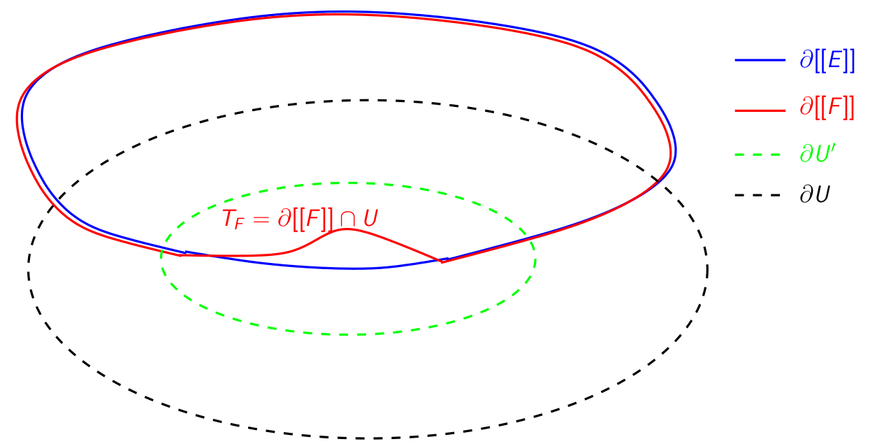
Figure 7: The reason for set $E_{U}$ is to guarantee there exists a cubical cover of the difference $[[F]]-[[E]]$ such that it is supported in some $U^{\prime}\subset\subset U$, then we can apply compactness theorem.

Remark 3.1.7 (Shared Boundaries).

We say that a set of currents in $\{T_{i}\}_{i=1}^{N}\subset\mathcal{E}_{U}$ have shared boundaries when $\partial T_{i}=\partial T_{j}$ for all $i\neq j$. By design, every subset of currents in $\mathcal{E}_{U}$ has shared boundaries.

Definition 3.1.8 (Precise Representative of $f$. [25]).

Assume $f\in L_{loc}^{1}(\mathbb{R}^{n})$, then

$$f^{*}(x)=\left\{\begin{array}[]{ll}\lim\limits_{r\rightarrow 0}\frac{1}{\alpha(n)r^{n}}\int_{B(x,r)}f(y)dy,&\quad\mbox{if this limit exist}\\ 0,&\quad otherwise.\end{array}\right.$$

Definition 3.1.9 (Precise Representative of a set $E$).

Let $E\in\mathbb{R}^{d}$ be a bounded set with finite perimeter, and $f=\chi_{E}$. Define

$$E^{*}=\{x|f^{*}(x)=1\},$$

to be the precise representative $E$.

Remark 3.1.10.

Since Hausdorff measure is a Radon measure, by Lebesgue Besicovitch differentiation theorem, the limit defined in 3.1.8 exists almost everywhere, i.e. $\mathcal{H}^{d}(E^{*}-E)=0.$ Compared to $E$, $E^{*}$ removed the subset from $E$ that cannot be seen under measure $\mathcal{H}^{d}.$

Definition 3.1.11 (Envelope).

The envelope ${\bf{Env}}(\{T_{i}\}_{i=1}^{N})$ of a set of integral currents with shared boundaries, $\{T_{i}\}_{i=1}^{N}\subset\mathcal{E}_{U}$, is defined as the union of $E^{*}_{i,j}$, $i<j$, such that $\partial\left(m\,\hbox{\vrule height=6.0pt,depth=0.0pt\vrule height=0.4pt,depth=0.0pt,width=5.0pt}\,[[E_{i,j}]]\right)=T_{i}-T_{j}$, where $|m(x)|=1$ for all $x\in E$. ${\bf{Env}}(\{T_{i}\}_{i=1}^{N})$ is the union of all the precise representatives of regions that lie between any two of the input currents.

Remark 3.1.12 (Compact support).

We note that for any finite collection of currents in $\mathcal{E}_{U}$, $\{T_{i}\}_{i=1}^{N}\subset\mathcal{E}_{U}$, we have that ${\bf{Env}}(\{T_{i}\}_{i=1}^{N})\subset\subset U$. Moreover, $\partial[[E^{*}_{ij}]]=\partial[[E]]$ as $\mathcal{H}^{d}(E^{*}-E)=0.$

Subclass we will minimize over:

In this section, we always work with $p$-currents in $\mathcal{E}_{U}$, and in particular, with sets of input currents $\{T_{i}\}_{i=1}^{N}\subset\mathcal{E}_{U}$. We will also assume that $\lambda$ is always small enough that the flat norm decomposition implicit in $\mathbb{F}_{\lambda}(T-T_{i})$ chooses an $S$ such that $T-T_{i}=\partial S$. Under this setting, we specialize the median functional (introduced in Equation 2) to the following one:

Definition 3.1.13 (Median).

Let $\{T_{i}\}_{i=1}^{N}\subset\mathcal{E}_{U}$. Then the median $\hat{T}_{\lambda}$ is defined to be

$$\hat{T}_{\lambda}=\operatornamewithlimits{argmin}_{T\in\mathcal{E}_{U}}\sum_{i=1}^{N}\mathbb{F}_{\lambda}(T-T_{i}).$$

Remark 3.1.14 ( $\hat{T}_{\lambda}\in\mathcal{E}_{U}$).

We need to prove that the integral current we get in the existence theorem is in fact also in $\mathcal{E}_{U}$, but we will get this fairly easily using the compactness theorem for sets of finite perimeter.

3.1.2 Outline of the section

We begin by showing that the difference current between the support of the median and the support of any input current, is a subset of the envelope we defined above. That is, if $T_{i}=\partial[[E_{i}]]\,\hbox{\vrule height=6.0pt,depth=0.0pt\vrule height=0.4pt,depth=0.0pt,width=5.0pt}\,U$ and $\hat{T}=\partial[[\hat{E}]]\,\hbox{\vrule height=6.0pt,depth=0.0pt\vrule height=0.4pt,depth=0.0pt,width=5.0pt}\,U$ then $[[E_{i}]]-[[\hat{E}]]$ is supported in ${\bf{Env}}(\{T_{i}\}_{i=1}^{N})$. Then, using the deformation theorem, we show that medians exist. This turns out to be a non-trivial result because there can indeed be minimizing sequences with unbounded mass. Next we demonstrate that for the case we are considering in this section—the codimension $1$ case—nice, smooth input currents can generate families of medians, all of which are non-smooth. Finally, we study the case of the mass-regularized median (as defined in Equation 4), and show that the difference set for this median lives in an $\epsilon$-neighborhood of the envelope of the input currents and that $\epsilon\rightarrow 0$ as $\mu/\lambda\rightarrow 0$.

3.2 Medians Are In The Envelope

Theorem 3.2.1 (Medians are in the envelope).

Let $\{T_{i}\}_{i=1}^{N}\subset\mathcal{E}_{U}$. The support any median, $\hat{T}_{\lambda}$, satisfies $\operatorname{supp}(\hat{T}_{\lambda}-T_{i})\subset Closure({\bf{Env}}(\{T_{i}\}_{i=1}^{N}))$ and

$$\hat{T}_{\lambda}\,\hbox{\vrule height=6.0pt,depth=0.0pt\vrule height=0.4pt,depth=0.0pt,width=5.0pt}\,\operatorname{Closure}({\bf{Env}}(\{T_{i}\}_{i=1}^{N}))^{c}=T_{i}\,\hbox{\vrule height=6.0pt,depth=0.0pt\vrule height=0.4pt,depth=0.0pt,width=5.0pt}\,\operatorname{Closure}({\bf{Env}}(\{T_{i}\}_{i=1}^{N}))^{c}\ \forall i.$$

.

Proof.

It is obvious that $\hat{T}_{\lambda}\,\hbox{\vrule height=6.0pt,depth=0.0pt\vrule height=0.4pt,depth=0.0pt,width=5.0pt}\,\operatorname{Closure}({\bf{Env}}(\{T_{i}\}_{i=1}^{N}))^{c}=T_{i}\,\hbox{\vrule height=6.0pt,depth=0.0pt\vrule height=0.4pt,depth=0.0pt,width=5.0pt}\,\operatorname{Closure}({\bf{Env}}(\{T_{i}\}_{i=1}^{N}))^{c}$ for all $i$ since all $T_{i}$’s agree outside ${\bf{Env}}(\{T_{i}\}_{i=1}^{N})^{c}.$ Now by way of contradiction, suppose $\operatorname{supp}(\hat{T}_{\lambda}-T_{i})\nsubseteq\operatorname{Closure}({\bf{Env}}(\{T_{i}\}_{i=1}^{N}))$, then the Hausdorff distance between $\operatorname{supp}(\hat{T}_{\lambda}-T_{i})$ and $\operatorname{Closure}({\bf{Env}}(\{T_{i}\}_{i=1}^{N}))$ is positive, i.e. $d_{H}(\hat{T}_{\lambda}-T_{i},{\bf{Env}}(\{T_{i}\}_{i=1}^{N}))=c>0$ for any $i$. For any $i$, define $[[S_{i}]]$ to be the unique bounded integral current that spans $\hat{T}_{\lambda}-T_{i}$. Note that because $\hat{T}_{\lambda}-T_{i}$ is codimension $1$ and bounded, it divides the space into two components, one of which is bounded and the other unbounded. The bounded component is the unique minimal current spanning $\hat{T}_{\lambda}-T_{i}$. In other words, $\partial[[S_{i}]]=\hat{T}_{\lambda}-T_{i}$ and

$$\partial([[S_{i}]]-[[S_{j}]])=\partial[[S_{i}]]-\partial[[S_{j}]]=T_{j}-T_{i}.$$

This implies $[[S_{i}]]-[[S_{j}]]$ spans $T_{i}-T_{j}$. Recall that in the definition of ${\bf{Env}}(\{T_{i}\}_{i=1}^{N})$, $\partial[[E^{*}_{ij}]]=T_{i}-T_{j}\subset{\bf{Env}}(\{T_{i}\}_{i=1}^{N})$. This tells us $[[S_{i}]]$ and $[[S_{j}]]$ agree outside ${\bf{Env}}(\{T_{i}\}_{i=1}^{N})$ almost everywhere, i.e.

$$\mathcal{H}^{p+1}((S_{i}\backslash{\bf{Env}}(\{T_{i}\}_{i=1}^{N}))\triangle(S_{j}\backslash{\bf{Env}}(\{T_{i}\}_{i=1}^{N})))=0,\ \forall i,j.$$

Define

$$S^{\prime}_{i} =S_{i}\,\hbox{\vrule height=6.0pt,depth=0.0pt\vrule height=0.4pt,depth=0.0pt,width=5.0pt}\,{\bf{Env}}(\{T_{i}\}_{i=1}^{N}),$$

$$S =S_{i}\,\hbox{\vrule height=6.0pt,depth=0.0pt\vrule height=0.4pt,depth=0.0pt,width=5.0pt}\,{\bf{Env}}(\{T_{i}\}_{i=1}^{N})^{c},$$

where the orientation of $[[S^{\prime}_{i}]]$ and $[[S]]$ are induced by $[[S_{i}]]$. Notice that even though it is possible for $S_{i}\,\hbox{\vrule height=6.0pt,depth=0.0pt\vrule height=0.4pt,depth=0.0pt,width=5.0pt}\,{\bf{Env}}(\{T_{i}\}_{i=1}^{N})^{c}\neq S_{j}\,\hbox{\vrule height=6.0pt,depth=0.0pt\vrule height=0.4pt,depth=0.0pt,width=5.0pt}\,{\bf{Env}}(\{T_{i}\}_{i=1}^{N})^{c}$ on a set of $\mathcal{H}^{p+1}-$measure 0 for $i\neq j$, $[[S]]$ as a current for any $i,j$ will be the same. Define the new median to be $\hat{T}^{\prime}_{\lambda}=\hat{T}_{\lambda}-\partial[[S]].$

Figure 8: The region outside the envelope is invariant with respect to input currents

Figure 9: Project $\hat{T}_{\lambda}$ out of the envelope back to the boundary of the envelope.

Then

$$\mathbb{F}_{\lambda}(\hat{T}_{\lambda}-T_{i}) =\lambda\operatorname{M}([[S_{i}]])$$

$$\mathbb{F}_{\lambda}(\hat{T}^{\prime}_{\lambda}-T_{i}) =\lambda\operatorname{M}([[S^{\prime}_{i}]]),$$

and $\operatorname{M}([[S_{i}]])-\operatorname{M}([[S^{\prime}_{i}]])=\operatorname{M}([[S]])\geq 0$ for each $i$. Therefore

$$\sum_{i=1}^{N}\mathbb{F}_{\lambda}(\hat{T}_{\lambda}-T_{i})-\mathbb{F}_{\lambda}(\hat{T}^{\prime}_{\lambda}-T_{i})=N\lambda\operatorname{M}([[S]])>0,$$

which contradicts the fact of $\hat{T}_{\lambda}$ being the median. So $\operatorname{supp}(\hat{T}_{\lambda}-T_{i})\subset\operatorname{Closure}({\bf{Env}}(\{T_{i}\}_{i=1}^{N})).$

∎

3.3 Medians Exist

Theorem 3.3.1 (Medians exists).

Let $\{T_{i}\}_{i=1}^{N}\subset\mathcal{E}_{U}$, where $\mathcal{E}_{U}$ is specified in Definition 3.1.6. Then $\hat{T}_{\lambda}$ exists, and $\hat{T}_{\lambda}\in\mathcal{E}_{U}$.

Proof.

The proof will be divided into the following steps:

1. Construct a sequence of cubical grids, $\{\operatorname{grid}\{\epsilon_{s}\}\}_{s=1}^{\infty}$, with side length $2\epsilon_{s}$ for each cube, such that

   $${\bf{Env}}(\{T_{i}\}_{i=1}^{N})\subset\operatorname{grid}(\epsilon_{s})\subset U,$$

   where $\epsilon_{s}\rightarrow 0$ as $s\rightarrow\infty$ and $\bigcap_{s=1}^{\infty}\operatorname{grid}(\epsilon_{s})=\operatorname{Closure}({\bf{Env}}(\{T_{i}\}_{i=1}^{N})).$
   

   Since there are finite number of input currents, there exists a $U^{\prime}\subset\subset U$ such that the difference of $T_{i}$’s only occurs in $U^{\prime}$. Let $R=\operatorname{hdist}(U^{\prime},U)$, where $\operatorname{hdist}$ is the Hausdorff distance. Define a sequence of cubical grid with side length $2\epsilon_{s}<R$, denoted as $\{grid(\epsilon_{s})\}_{s=1}^{\infty}$, such that

   $${\bf{Env}}(\{T_{i}\}_{i=1}^{N})\subset\operatorname{grid}(\epsilon_{s})\subset U.$$

   Moreover each cube in $\operatorname{grid}(\epsilon_{s})$ has nonempty intersection with ${\bf{Env}}(\{T_{i}\}_{i=1}^{N})$. Therefore

   $$\lim\limits_{s\rightarrow\infty}\operatorname{grid}(\epsilon_{s})=\bigcap_{s=1}^{\infty}\operatorname{grid}(\epsilon_{s})={\bf{Env}}(\{T_{i}\}_{i=1}^{N}).$$

   By the definition of ${\bf{Env}}(\{T_{i}\}_{i=1}^{N})$, the differences between input currents lie within ${\bf{Env}}(\{T_{i}\}_{i=1}^{N})$, i.e.,

   $$T_{i}\,\hbox{\vrule height=6.0pt,depth=0.0pt\vrule height=0.4pt,depth=0.0pt,width=5.0pt}\,{\bf{Env}}(\{T_{i}\}_{i=1}^{N})^{c}=T_{j}\,\hbox{\vrule height=6.0pt,depth=0.0pt\vrule height=0.4pt,depth=0.0pt,width=5.0pt}\,{\bf{Env}}(\{T_{i}\}_{i=1}^{N})^{c},\forall i,j.$$

   And ${\bf{Env}}(\{T_{i}\}_{i=1}^{N})\subset\operatorname{grid}(\epsilon_{s})$, so $T_{i}$’s also agrees outside $\operatorname{grid}(\epsilon_{s})$ for all $s$.

2. Push each $T_{i}$ to $\operatorname{grid}(\epsilon_{s})$.
   

   Since all $T_{i}$’s agrees outside the ${\bf{Env}}(\{T_{i}\}_{i=1}^{N})$ and ${\bf{Env}}(\{T_{i}\}_{i=1}^{N})\subset\operatorname{grid}(\epsilon_{s})$, we only need to push $T_{i}\,\hbox{\vrule height=6.0pt,depth=0.0pt\vrule height=0.4pt,depth=0.0pt,width=5.0pt}\,\operatorname{grid}(\epsilon_{s})$ to the grid. Hence we do not have to decide how $\partial T_{i}$ gets pushed.

   By the deformation theorem [45, Theorem 5.1], each $T_{i}\,\hbox{\vrule height=6.0pt,depth=0.0pt\vrule height=0.4pt,depth=0.0pt,width=5.0pt}\,\operatorname{grid}(\epsilon_{s})$ can be decomposed into

   $$T_{i}\,\hbox{\vrule height=6.0pt,depth=0.0pt\vrule height=0.4pt,depth=0.0pt,width=5.0pt}\,\operatorname{grid}(\epsilon_{s})=T^{\pi}_{i}(\epsilon_{s})\,\hbox{\vrule height=6.0pt,depth=0.0pt\vrule height=0.4pt,depth=0.0pt,width=5.0pt}\,\operatorname{grid}(\epsilon_{s})+\partial S^{\pi}_{i}(\epsilon_{s})$$

   where $T^{\pi}_{i}(\epsilon_{s})\,\hbox{\vrule height=6.0pt,depth=0.0pt\vrule height=0.4pt,depth=0.0pt,width=5.0pt}\,\operatorname{grid}(\epsilon_{s})\in\mathcal{P}_{p}\mathbb{R}^{p+1}$, the space of polyhedral $p$-currents in $\mathbb{R}^{p+1}$, and $S^{\pi}_{i}(\epsilon_{s})\in\mathcal{I}_{p+1}\mathbb{R}^{p+1}$, the space of integral $(p+1)$-currents in $\mathbb{R}^{p+1}$. In addition,

   $$\operatorname{M}(T_{i}^{\pi}(\epsilon_{k})\,\hbox{\vrule height=6.0pt,depth=0.0pt\vrule height=0.4pt,depth=0.0pt,width=5.0pt}\,\operatorname{grid}(\epsilon_{s})) \leq\gamma\operatorname{M}(T_{i}\,\hbox{\vrule height=6.0pt,depth=0.0pt\vrule height=0.4pt,depth=0.0pt,width=5.0pt}\,\operatorname{grid}(\epsilon_{s})),$$

   $$T^{\pi}_{i}(\epsilon_{s})\,\hbox{\vrule height=6.0pt,depth=0.0pt\vrule height=0.4pt,depth=0.0pt,width=5.0pt}\,\operatorname{grid}^{c}(\epsilon_{s}) =T_{i}\,\hbox{\vrule height=6.0pt,depth=0.0pt\vrule height=0.4pt,depth=0.0pt,width=5.0pt}\,\operatorname{grid}^{c}(\epsilon_{s}),$$

   where $\gamma=2(p+1)^{2p+2}$.

   Define

   $$T^{\pi}_{i}(\epsilon_{s})=T^{\pi}_{i}(\epsilon_{s})\,\hbox{\vrule height=6.0pt,depth=0.0pt\vrule height=0.4pt,depth=0.0pt,width=5.0pt}\,\operatorname{grid}(\epsilon_{s})+T_{i}\,\hbox{\vrule height=6.0pt,depth=0.0pt\vrule height=0.4pt,depth=0.0pt,width=5.0pt}\,\operatorname{grid}^{c}(\epsilon_{s}).$$

   As a consequence,

   $$\begin{aligned} \operatorname{M}(T_{i}^{\pi}(\epsilon_{s}))&=\operatorname{M}(T^{\pi}_{i}\,\hbox{\vrule height=6.0pt,depth=0.0pt\vrule height=0.4pt,depth=0.0pt,width=5.0pt}\,\operatorname{grid}(\epsilon_{s}))+\operatorname{M}(T^{\pi}_{i}\,\hbox{\vrule height=6.0pt,depth=0.0pt\vrule height=0.4pt,depth=0.0pt,width=5.0pt}\,\operatorname{grid}^{c}(\epsilon_{s}))\\ &\leq\gamma\operatorname{M}(T_{i}\,\hbox{\vrule height=6.0pt,depth=0.0pt\vrule height=0.4pt,depth=0.0pt,width=5.0pt}\,\operatorname{grid}(\epsilon_{s}))+\operatorname{M}(T_{i}\,\hbox{\vrule height=6.0pt,depth=0.0pt\vrule height=0.4pt,depth=0.0pt,width=5.0pt}\,\operatorname{grid}^{c}(\epsilon_{s}))\\ &\leq(\gamma+1)\operatorname{M}(T_{i}),~{}~{}~{}\mbox{ and }\\ \end{aligned}$$ (5)

   $$\begin{aligned} \mathbb{F}_{\lambda}(T_{i}-T_{i}^{\pi}(\epsilon_{s}))&=\mathbb{F}_{\lambda}(T_{i}\,\hbox{\vrule height=6.0pt,depth=0.0pt\vrule height=0.4pt,depth=0.0pt,width=5.0pt}\,\operatorname{grid}(\epsilon_{s})-T^{\pi}_{i}(\epsilon_{s}))\,\hbox{\vrule height=6.0pt,depth=0.0pt\vrule height=0.4pt,depth=0.0pt,width=5.0pt}\,\operatorname{grid}(\epsilon_{s}))\\ &=\mathbb{F}_{\lambda}(\partial S_{i}^{\pi}(\epsilon_{s}))\\ &\leq\epsilon_{s}\gamma\operatorname{M}(T_{i}\,\hbox{\vrule height=6.0pt,depth=0.0pt\vrule height=0.4pt,depth=0.0pt,width=5.0pt}\,\operatorname{grid}(\epsilon_{s}))\\ &\leq\epsilon_{s}\gamma\operatorname{M}(T_{i})\,.\end{aligned}$$ (6)

3. Construct pushed minimizing sequence for medians.
   

   Let $\{\hat{T}_{\lambda,j}\}\subset\mathcal{E}_{U}$ be a minimizing sequence for the median objective function. Since all $T_{i}$’s agree outside $\operatorname{grid}(\epsilon_{s})$, we can restrict $\{\hat{T}_{\lambda,j}\}$ to satisfy

   $$\hat{T}_{\lambda,j}\,\hbox{\vrule height=6.0pt,depth=0.0pt\vrule height=0.4pt,depth=0.0pt,width=5.0pt}\,\operatorname{grid}^{c}(\epsilon_{s})=T_{i}\,\hbox{\vrule height=6.0pt,depth=0.0pt\vrule height=0.4pt,depth=0.0pt,width=5.0pt}\,\operatorname{grid}^{c}(\epsilon_{s}),\ \forall i,j.$$

   Next we first push each $\hat{T}_{\lambda,j}$ to $grid(\epsilon_{s})$, denoted as $\hat{T}^{\pi}_{\lambda,j}(\epsilon_{s})\,\hbox{\vrule height=6.0pt,depth=0.0pt\vrule height=0.4pt,depth=0.0pt,width=5.0pt}\,\operatorname{grid}(\epsilon_{s})$ and then extend it to $U$ as

   $$\hat{T}^{\pi}_{\lambda,j}(\epsilon_{s})=\hat{T}^{\pi}_{\lambda,j}(\epsilon_{s})\,\hbox{\vrule height=6.0pt,depth=0.0pt\vrule height=0.4pt,depth=0.0pt,width=5.0pt}\,\operatorname{grid}(\epsilon_{s})+T_{i}\,\hbox{\vrule height=6.0pt,depth=0.0pt\vrule height=0.4pt,depth=0.0pt,width=5.0pt}\,\operatorname{grid}^{c}(\epsilon_{s}).$$

   Note

   $$\hat{T}_{\lambda,j}\,\hbox{\vrule height=6.0pt,depth=0.0pt\vrule height=0.4pt,depth=0.0pt,width=5.0pt}\,\operatorname{grid}^{c}(\epsilon_{s})=\hat{T}^{\pi}_{\lambda,j}(\epsilon_{s})\,\hbox{\vrule height=6.0pt,depth=0.0pt\vrule height=0.4pt,depth=0.0pt,width=5.0pt}\,\operatorname{grid}^{c}(\epsilon_{s})=T_{i}\,\hbox{\vrule height=6.0pt,depth=0.0pt\vrule height=0.4pt,depth=0.0pt,width=5.0pt}\,\operatorname{grid}^{c}(\epsilon_{s})=T_{i}^{\pi}(\epsilon_{s})\,\hbox{\vrule height=6.0pt,depth=0.0pt\vrule height=0.4pt,depth=0.0pt,width=5.0pt}\,\operatorname{grid}^{c}(\epsilon_{s}).$$

   In particular, we will pick $\epsilon_{s}=\frac{1}{2^{s}w_{s}}$, where $\omega_{s}=\operatorname{M}^{p}(\hat{T}_{\lambda,j}).$

4. Modify $\hat{T}^{\pi}_{\lambda,j}(\epsilon_{s})$ to $\hat{T}^{adj}_{\lambda,j}$.
   

   After pushing everything to the grid, we can treat all $\{T_{i}^{\pi}(\epsilon_{s})\}$ and $\{\hat{T}^{\pi}_{\lambda,j}(\epsilon_{s})\}$ as the boundaries of sets $\{E^{\pi}_{i}(\epsilon_{s})\cap U\}$ and $\{\hat{E}^{\pi}_{\lambda,j}(\epsilon_{s})\cap U\}$, and the flat norm between $T^{\pi}_{i}(\epsilon_{s})$ and $\hat{T}^{\pi}_{\lambda,j}(\epsilon_{s})$ is

   $$\begin{aligned} \mathbb{F}_{\lambda}(\hat{T}^{\pi}_{\lambda,j}(\epsilon_{s})-T^{\pi}_{i}(\epsilon_{s}))&=\mathcal{H}^{p+1}((\hat{E}^{\pi}_{\lambda,j}(\epsilon_{s})\cap U)\triangle(E^{\pi}_{i}(\epsilon_{s})\cap U))\\ &=\mathcal{H}^{p+1}(\mbox{union of cubes in $(\hat{E}^{\pi}_{\lambda,j}(\epsilon_{s})\cap U)\triangle(E^{\pi}_{i}(\epsilon_{s})\cap U)$})\\ &=(2\epsilon_{s})^{p+1}(\mbox{union of cubes in $(\hat{E}^{\pi}_{\lambda,j}(\epsilon_{s})\cap U)\triangle(E^{\pi}_{i}(\epsilon_{s})\cap U)$}).\end{aligned}$$ (7)

   For each $\hat{T}^{\pi}_{\lambda,j}(\epsilon_{s})$, we can modify $\hat{T}^{\pi}_{\lambda,j}(\epsilon_{s})$ by adding cubes $\mathcal{C}$ to $\hat{E}^{\pi}_{\lambda,j}(\epsilon_{s})$ or subtracting cubes $\mathcal{C}$ from $\hat{E}^{\pi}_{\lambda,j}(\epsilon_{s})$ and replace the old $\hat{T}^{\pi}_{\lambda,j}(\epsilon_{s})$ with $\hat{T}^{\pi}_{\lambda,j}+\sum_{C\in\mathcal{C}}\partial C$, denoted as $\hat{T}^{adj}_{\lambda,j}(\epsilon_{s})$, until it is the union of pieces from $\{T^{\pi}_{i}(\epsilon_{s})\}$.

   Now in more detail: the intersections of the $E^{\pi}_{i}(\epsilon_{s})\cap\operatorname{grid}(\epsilon_{s})$ partition $\operatorname{grid}(\epsilon_{s})$ into a finite number of components that sometimes share boundaries. For each component $\operatorname{Comp}_{l}(\epsilon_{s})$,

   1. If $\operatorname{Comp}_{l}(\epsilon_{s})\cap\hat{E}^{\pi}_{\lambda,j}(\epsilon_{s})=\emptyset$, do nothing;

   2. If $\operatorname{Comp}_{l}(\epsilon_{s})\cap\hat{E}^{\pi}_{\lambda,j}(\epsilon_{s})\neq\emptyset$, we will update $\hat{T}^{\pi}_{\lambda,j}(\epsilon_{s})$ in the following way:

      Define

      • $\operatorname{Comp}_{l}(\epsilon_{s})\cap\hat{E}_{\lambda,j}(\epsilon_{s})=F_{l}(\epsilon_{s})$,

      • $\operatorname{Comp}_{l}(\epsilon_{s})\cap\hat{E}^{c}_{\lambda,j}(\epsilon_{s})=K_{l}(\epsilon_{s}).$

      Note that $F_{l}(\epsilon_{s})\cup K_{l}(\epsilon_{s})=\operatorname{Comp}_{l}(\epsilon_{s})$ and either $E^{\pi}_{i}(\epsilon_{s})\cap\operatorname{Comp}_{l}(\epsilon_{s})=\emptyset$ or $\#E^{\pi}_{i}(\epsilon_{s})\cap\operatorname{Comp}_{l}(\epsilon_{s})=\#\operatorname{Comp}_{l}(\epsilon_{s})$. The second condition means if $\operatorname{Comp}_{l}(\epsilon_{s})$ contains one of the cubes from $E^{\pi}_{i}(\epsilon_{s})$, then all the cubes in $\operatorname{Comp}_{l}(\epsilon_{s})$ are contained $E^{\pi}_{i}(\epsilon_{s})$. As a result,

      $$\hat{E}^{\pi}_{\lambda,j}\triangle E^{\pi}_{i}(\epsilon_{s})=F_{l}(\epsilon_{s})\ or\ K_{l}(\epsilon_{s}).$$

      Now for each cube $C$ in $F_{l}(\epsilon_{s})$ or $K_{l}(\epsilon_{s})$, denote

      1. $N_{C}^{F_{l}(\epsilon_{s})}=\#\{E^{\pi}_{i}(\epsilon)|C\in E^{\pi}_{i}(\epsilon)\}$ if $C\in F_{l}(\epsilon_{s})$,

      2. $N_{C}^{K_{l}(\epsilon_{s})}=\#\{E^{\pi}_{i}(\epsilon)|C\in E^{\pi}_{i}(\epsilon)\}$ if $C\in K_{l}(\epsilon_{s})$.

      There are two cases:

      1. If $\sum_{C\in F_{l}(\epsilon_{s})}N_{C}^{F_{l}(\epsilon_{s})}\geq\sum_{C\in K_{l}(\epsilon_{s})}N_{C}^{K_{l}(\epsilon_{s})}$, then subtracting $\operatorname{Comp}_{l}(\epsilon_{s})$ will decrease the sum of flat norms between $\hat{T}_{\lambda,j}(\epsilon_{s})$ and $T^{\pi}_{i}(\epsilon_{s})$’s by $(2\epsilon_{s})^{p+1}\sum_{C\in F_{l}(\epsilon_{s})}N_{C}^{F_{l}(\epsilon_{s})}$ and increase the sum by $(2\epsilon_{s})^{p+1}\sum_{C\in K_{l}(\epsilon_{s})}N_{C}^{K_{l}(\epsilon_{s})}$. Therefore, the sum of flat norms will decrease by $(2\epsilon_{s})^{p+1}(\sum_{C\in F_{l}(\epsilon_{s})}N_{C}^{F_{l}(\epsilon_{s})}-\sum_{C\in K_{l}(\epsilon_{s})}N_{C}^{K_{l}(\epsilon_{s})})$. So $\hat{E}^{adj}_{\lambda,j}(\epsilon_{s})=\hat{E}^{\pi}_{\lambda,j}(\epsilon_{s})\backslash\operatorname{Comp}_{l}(\epsilon_{s})$ and $\hat{T}^{adj}_{\lambda,j}(\epsilon_{s})=\hat{E}_{\lambda,j}(\epsilon_{s})-\sum_{C\in\hat{E}_{\lambda,j}(\epsilon_{s})\backslash\operatorname{Comp}_{l}(\epsilon_{s})}$ $\partial C$,

      2. If $\sum_{C\in F_{l}(\epsilon_{s})}N_{C}^{F_{l}(\epsilon_{s})}<\sum_{C\in K_{l}(\epsilon_{s})}N_{C}^{K_{l}(\epsilon_{s})}$, then adding $\operatorname{Comp}_{l}(\epsilon_{s})$ will decrease the sum of flat norms between $\hat{T}_{\lambda,j}(\epsilon_{s})$ and $T^{\pi}_{i}(\epsilon_{s})$’s by $(2\epsilon_{s})^{p+1}\sum_{C\in K_{l}(\epsilon_{s})}N_{C}^{K_{l}(\epsilon_{s})}$ and increase the sum by $(2\epsilon_{s})^{p+1}\sum_{C\in F_{l}(\epsilon_{s})}N_{C}^{F_{l}(\epsilon_{s})}$. Therefore, the sum of flat norms will decrease by $(2\epsilon_{s})^{p+1}(\sum_{C\in K_{l}(\epsilon_{s})}N_{C}^{K_{l}(\epsilon_{s})}-\sum_{C\in F_{l}(\epsilon_{s})}N_{C}^{F_{l}(\epsilon_{s})})$. So $\hat{E}^{adj}_{\lambda,j}(\epsilon_{s})=\hat{E}^{\pi}_{\lambda,j}(\epsilon_{s})\cup\operatorname{Comp}_{l}(\epsilon_{s})$ and $\hat{T}^{adj}_{\lambda,j}(\epsilon_{s})=\hat{E}^{\pi}_{\lambda,j}(\epsilon_{s})+\sum_{C\in\hat{E}_{\lambda,j}(\epsilon_{s})\backslash\operatorname{Comp}_{l}(\epsilon_{s})}\partial C$.

      The process will end in finite steps since there are only finite number of $\operatorname{Comp}_{l}(\epsilon_{s})$’s. And when it finishes, $\hat{E}_{\lambda,j}(\epsilon_{s})\,\hbox{\vrule height=6.0pt,depth=0.0pt\vrule height=0.4pt,depth=0.0pt,width=5.0pt}\,\operatorname{grid}(\epsilon_{s})$ will be the union of pieces from $T^{\pi}_{i}(\epsilon_{s})\,\hbox{\vrule height=6.0pt,depth=0.0pt\vrule height=0.4pt,depth=0.0pt,width=5.0pt}\,\operatorname{grid}(\epsilon_{s})$.

   \begin{picture}(19056.0,11724.0)(838.0,-10873.0)\end{picture}

   Figure 10: An example in the case of $p+1=2$ of how to adjust the pushed median.

   In the top-left picture of Figure 10, there are 3 pushed input currents represented as solid green, red and purple lines. The black dashed line is the original pushed median $\hat{T}_{\lambda,j}(\epsilon_{s})$. In the top-right picture, pink regions represent the regions outside $\hat{E}^{\pi}_{\lambda,j}(\epsilon_{s})$ while yellow regions are the opposite. The number in each cube $C$ equals $\#\{E^{\pi}_{i}(\epsilon)|C\in E^{\pi}_{i}(\epsilon)\}$. In the bottom-left picture, different color represents different connected components. For the blue component, it does not intersects with $\hat{E}^{\pi}_{\lambda,j}(\epsilon_{s})$, we leave it alone. For the red component, $\sum_{C\in F_{l}(\epsilon_{s})}N_{C}^{F_{l}(\epsilon_{s})}<\sum_{C\in K_{l}(\epsilon_{s})}N_{C}^{K_{l}(\epsilon_{s})}$, so we added the entire yellow component to $\hat{E}^{\pi}_{\lambda,j}(\epsilon_{s})$. For the green component, $\sum_{C\in F_{l}(\epsilon_{s})}N_{C}^{F_{l}(\epsilon_{s})}\geq\sum_{C\in K_{l}(\epsilon_{s})}N_{C}^{K_{l}(\epsilon_{s})}$, so we subtract the green component from $\hat{E}^{\pi}_{\lambda,j}(\epsilon_{s})$. We can continue the same process to cyan and purple components. In bottom-right picture, the black dashed line is the updated pushed median.

5. $\operatorname{M}(\hat{T}^{adj}_{\lambda,j}(\epsilon_{s}))$ is bounded uniformly.
   

   Each $\hat{T}^{adj}_{\lambda,j}(\epsilon_{s})\,\hbox{\vrule height=6.0pt,depth=0.0pt\vrule height=0.4pt,depth=0.0pt,width=5.0pt}\,\operatorname{grid}(\epsilon_{s})$ is the union of pieces from $T_{i}^{\pi}(\epsilon_{s})\,\hbox{\vrule height=6.0pt,depth=0.0pt\vrule height=0.4pt,depth=0.0pt,width=5.0pt}\,\operatorname{grid}(\epsilon_{s})$ and $\hat{T}^{adj}_{\lambda,j}(\epsilon_{s})\,\hbox{\vrule height=6.0pt,depth=0.0pt\vrule height=0.4pt,depth=0.0pt,width=5.0pt}\,\operatorname{grid}^{c}(\epsilon_{s})=T_{i}^{\pi}(\epsilon_{s})\,\hbox{\vrule height=6.0pt,depth=0.0pt\vrule height=0.4pt,depth=0.0pt,width=5.0pt}\,\operatorname{grid}^{c}(\epsilon_{s})$, so

   $$\operatorname{M}(\hat{T}^{adj}_{\lambda,j}(\epsilon_{s})) \leq\sum_{i=1}^{N}\operatorname{M}(T_{i}^{\pi}(\epsilon_{s}))\leq\sum_{i=1}^{N}(\gamma+1)\operatorname{M}(T_{i}),$$

   and $\hat{T}^{adj}_{\lambda}(\epsilon_{s})\in\mathcal{E}_{U}$. $\{\hat{T}^{adj}_{\lambda,j}(\epsilon_{s})\}\subset U.$

6. Apply triangle inequality and prove that $\hat{T}^{adj}_{\lambda}(\epsilon_{s})$ converges to the median $\hat{T}_{\lambda}$ as $s\rightarrow\infty$.
   

   By diagonal argument, the sequence $\{\hat{T}^{adj}_{\lambda,s}(\epsilon_{s})\}$ converges to some $\hat{T}_{\lambda}.$

   Note that

   $$\mathbb{F}_{\lambda}(\hat{T}^{\pi}_{\lambda,s}-\hat{T}_{\lambda,s}) \leq\epsilon_{s}\gamma\operatorname{M}(\hat{T}_{\lambda,s})\leq\frac{\gamma}{2^{s}},$$ (8)

   $$\sum_{i=1}^{N}\mathbb{F}_{\lambda}(\hat{T}^{adj}_{\lambda,s}(\epsilon_{s})-T_{i}) \leq\sum_{i=1}^{N}\mathbb{F}_{\lambda}(\hat{T}^{\pi}_{\lambda,s}(\epsilon_{s})-T_{i}).$$ (9)

   This inequality follows from the actions described in Step 4 for the construction of $\hat{T}^{adj}_{\lambda,s}(\epsilon_{s})$, where the adjustment process decreases the sum of flat norms between all $T_{i}$’s.

   Using the triangle inequality with the bounds in Equations 8 and 9 we get

   $$\lim_{s\rightarrow\infty}\sum_{i=1}^{N}\mathbb{F}_{\lambda}(\hat{T}_{\lambda,s}-T_{i}) \leq\sum_{i=1}^{N}\mathbb{F}_{\lambda}(\hat{T}_{\lambda}-T_{i})$$

   $$\leq\lim_{s\rightarrow\infty}\sum_{i=1}^{N}\mathbb{F}_{\lambda}(\hat{T}^{adj}_{\lambda,s}(\epsilon_{s})-T_{i})$$

   $$\leq\lim_{s\rightarrow\infty}\sum_{i=1}^{N}[(\mathbb{F}_{\lambda}(\hat{T}^{adj}_{\lambda,s}(\epsilon_{s})-T^{\pi}_{i}(\epsilon_{s}))+(\mathbb{F}_{\lambda}(T^{\pi}_{i}(\epsilon_{s})-T_{i}))]$$

   $$\leq\lim_{s\rightarrow\infty}\sum_{i=1}^{N}[(\mathbb{F}_{\lambda}(\hat{T}^{\pi}_{\lambda,s}(\epsilon_{s})-T^{\pi}_{i}(\epsilon_{s}))+(\mathbb{F}_{\lambda}(T^{\pi}_{i}(\epsilon_{s})-T_{i}))]$$

   $$\leq\lim_{s\rightarrow\infty}\sum_{i=1}^{N}[\mathbb{F}_{\lambda}(\hat{T}^{\pi}_{\lambda,s}(\epsilon_{s})-\hat{T}_{\lambda,s})+\mathbb{F}_{\lambda}(\hat{T}_{\lambda,s}-T_{i})+2(\mathbb{F}_{\lambda}(T^{\pi}_{i}(\epsilon_{s})-T_{i}))]$$

   $$\leq\lim_{s\rightarrow\infty}\left[\sum_{i=1}^{N}\mathbb{F}_{\lambda}(\hat{T}_{\lambda,s}-T_{i})+\frac{\gamma N}{2^{s}}+\epsilon_{s}\gamma\sum_{i=1}^{N}\operatorname{M}(T_{i})\right]$$

   $$=\lim_{s\rightarrow\infty}\sum_{i=1}^{N}\mathbb{F}_{\lambda}(\hat{T}_{\lambda,s}-T_{i})\,.$$

   Therefore $\hat{T}_{\lambda}$ is a median and by step 5, $\operatorname{M}(\hat{T}_{\lambda})\leq\sum_{i=1}^{N}(\gamma+1)\operatorname{M}(T_{i})$ and $\hat{T}_{\lambda}\in\mathcal{E}_{U}$.

∎

3.4 Medians Can Be Wild

As we proved in Section 3.3, the median $\hat{T}_{\lambda}$ for $\{T_{i}\}_{i=1}^{N}\subset\mathcal{E}_{U}$ always exists with a mass bounded by $\sum_{i=1}^{N}(\gamma+1)\operatorname{M}(T_{i})$. However, it is not guaranteed that all the medians are bounded. In fact, there exist sequences of medians whose masses diverge. For example, take two input currents $T_{1}$ and $T_{2}$ to be the upper and lower half of the boundary of a rectangle. The median $\hat{T}_{\lambda}$ can be any non self-intersecting curve of finite length inside the square. We can, for example use any graph that represents a random walk in the vertical direction vesus time, represented by the horizontal axis, under the constriant that the walk must stay in the rectangle. Of course the lengths (i.e. mass) of these random walks are not bounded since the speed of the walk (the slope of the graph) is not bounded.

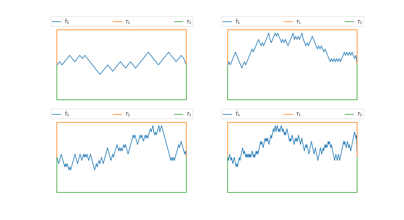
Figure 11: Random walk medians can have arbitrarily high mass.

3.5 Smooth Inputs Can Generate Non-smooth Medians

Even if the input currents are regular, the median need not be regular. We present an example in $\mathbb{R}^{2}$ showing the median can fail to be regular. We will be looking for medians which are pieces of boundaries of sets, as we did in the proof of existence for the codimension-$1$ shared boundary case above.

Theorem 3.5.1.

(Regularity of inputs does not imply regularity of median) Suppose that each of the $T_{i}$’s are smooth, with shared boundaries, and that we minimize over $T$ that are pieces of boundaries of sets. Then the entire set of medians might consist only of currents that lack smoothness somewhere.

Proof.

Consider the case of the input $T_{i}$’s being oriented graphs of smooth functions $f_{i}$, where the {set, orienting vector field} pairs are given by:

$$\left(\{(x,f_{i}(x))|x\in[0,1]\},\frac{(-1,-f_{i}^{\prime}(x))}{\sqrt{1+(f_{i}^{\prime}(x))^{2}}}\right)$$

and each $f_{i}$ satisfies $f_{i}(0)=1=f_{i}(1)$. An example is shown in Figure 15.

The next lemma is more than we actually need, but is included because part of its proof anticipates a later proof.

Lemma 3.5.2.

(Graphs are Good) When the $T_{i}$’s are one-dimensional graphs in $\mathbb{R}^{2}$ sharing the same two boundary points, the infimum of the median objective functional over piece-wise smooth non-graphs is not smaller than the infimum over graphs. Hence the infimum in the median problem can be restricted to graphs.

Figure 12: Slicing $T_{i}$, $\hat{T}$ and $S_{i}$ with a vertical line, $h_{x}$.

Figure 13: Structure of the slice. The intervals generated by the intersection of $h_{x}$ and the $S_{i}$ are shown in red.

Figure 14: All the slices and intervals they generate.

Proof of Lemma 3.5.2.

Outline: We slice $T_{i}$, $\hat{T}$, and the $2$-dimensional current $S_{i}$ bounded by $T_{i}$ and $\hat{T}$ vertically to get positive and negative oriented $0$-currents and oriented intervals. Sum of the integrals of the lengths of those intervals over the $x$-axis equals the median objective function for $\hat{T}$:

$$\sum_{i=1}^{N}\mathbb{F}_{\lambda}(T_{i}-\hat{T})=\int\left(\sum_{i=1}^{N}\mathcal{H}^{1}(h_{x}\cap S_{i})\right)dx$$

where we are interpreting $S_{i}$ as the set we integrate over to get the current $S_{i}$. (We can also express this as $\sum_{i=1}^{N}\mathbb{F}_{\lambda}(T_{i}-\hat{T})=\sum_{i=1}^{N}\operatorname{M}(\hat{h}_{x}(S_{i}))$ where $\hat{h}_{x}(S_{i})$ is the slice of the current $S_{i}$ (which is itself a current) by the line $h_{x}$). The strategy of the proof shows that every sum equals or exceeds the sum generated by a graph that stays in the median interval of each slice. (Recall that in 1 dimension, the set of medians is either a point or an interval. If we minimize the median objective function over graphs, we get that the graph has to live in the median interval generated by the slicing of the $T_{i}$.) We see that if every slice of the median generates points not in the median interval of that slice, the cost exceeds the minimal cost. Since the minimal cost is attained by any graph that stays in the median intervals, and any such interval is forced to stay in a cone with a kink, we are done.

Now, the details:

1. We assume that the median intersects vertical slices transversely almost everywhere.

   1. This can be shown by assuming not – that the measure of $E$, defined to be the $x$’s such that $h_{x}$ intersects $\hat{T}$ tangentially at some point, has positive measure. Choose any (big) $C>0$.

   2. We can cover $E$ with intervals $F_{w}$, $w\in E$ which are in one to one correspondence with disjoint pieces of $\hat{T}$, $G_{w}$, such that $\mathcal{H}^{1}(G_{w})>C\mathcal{H}^{1}(F_{w})$.

   3. This implies that the length of $\hat{T}$ is unbounded.

   4. Note: We use the fact that $\hat{T}$ is piecewise smooth, so the projection of the points on $\hat{T}$ where it is not smooth has measure zero on the $x$ axis.

2. We assume that the $T_{i}$ all intersect the vertical slices transversely.

3. Since the mass of $T_{i}$ and $\hat{T}$ is finite, the slice $h_{x}$ generates a finite number of intersections with $\hat{T}$ for almost every $x$.

4. As a result, for almost every $x$, $\mathcal{H}^{0}(h_{x}\cap\hat{T})=2m(x)+1$, each intersection with multiplicity and orientation of either $+1$ or $-1$. We will denote the intersection points $y_{i}$ $i=1,...,2m(x)+1$ This is shown in Figures 12 and 13.

5. Note: we will abbreviate $m(x)$ to $m$ from this point on in this proof.

6. The $2m+1$ points generate the $2m+2$ intervals $I_{0}=(-\infty,y_{0})$, $I_{1}=[y_{1},y_{2})$, $I_{2}=[y_{2},y_{3})$, …, $I_{2m}=[y_{2m},y_{2m+1})$, $I_{2m+1}=[y_{2m+1},\infty)$.

7. Define $a_{j}\equiv|\{i|h_{x}\cap T_{i}\in I_{j}|$.

8. Figure 14 shows all slices generated at one x for a case in which there are $10$ input currents $T_{1}$,…,$T_{10}$.

9. Observe that there are two types of intervals: those with a positive left endpoint - $I_{1}$,$I_{3}$,…,$I_{2m-1}$, $I_{2m+1}$ – and those with a positive right endpoint – $I_{0}$,$I_{2}$,…,$I_{2m-2}$, $I_{2m}$.

10. Observe that, when $j\geq 2$ is even, then all the slices generate $\sum_{i=0}^{j-1}a_{i}$ red intervals and $a_{j}$ partial intervals from the right endpoint to the intersections of the $T_{i}$ and $I_{j}$. Likewise, one can see that when $j<2m+1$ is odd, all the slices generate $\sum_{i=j+1}^{2m+1}a_{i}$ red intervals and $a_{j}$ partial intervals from the $T_{i}$ generated points in $I_{j}$ and the positive endpoint of $I_{j}$.

11. In order that the intervals generated by the intersection of $h_{x}$ with all the $S_{i}$’s provide separate paths to every (green) intersection point and some fixed positive point in $y_{k}\in\{y_{1},y_{3},...y_{2m+1}\}$, four conditions must be met. We must have that in each interval $I_{l}$, l even and odd, to the left and right of $y_{k}$ a sufficient number of full red intervals to create separate paths to the green $T_{i}$ intersections that are in that interval (if their connecting partial interval connects in the wrong direction) or those further away. The four conditions thus generated are:

    1. For $l=k,k+2,...$ we must have

       $$\sum_{l+1}^{2m+1}a_{i}\geq\sum_{l+1}^{2m+1}a_{i}$$

    2. for $l=k-2,k-4,...$ we must have

       $$\sum_{l+1}^{2m+1}a_{i}\geq\sum_{i=0}^{l}a_{i}$$

    3. for $l=k+1,k+3,...$ we must have

       $$\sum_{i=0}^{l-1}a_{i}\geq\sum_{i=l}^{2m+1}a_{i}$$

    4. for $l=k-1,k-3,...$ we must have

       $$\sum_{i=0}^{l-1}a_{i}\geq\sum_{i=0}^{l-1}a_{i}$$

12. This reduces to finding $k\in\{1,3,5,...,2m-1,2m+1\}$ such that:

    1. in the case $k=1$:

       $$\sum_{i=0}^{k}a_{i} \geq \sum_{i=k+1}^{2m+1}a_{i}$$

    2. in the case that $k\in\{3,5,...,2m-1\}$:

       $$\sum_{i=0}^{k}a_{i} \geq \sum_{i=k+1}^{2m+1}a_{i}$$

       $$\sum_{i=k-1}^{2m+1}a_{i} \geq \sum_{i=0}^{k-2}a_{i}$$

    3. in the case that $k=2m+1$:

       $$\sum_{i=k-1}^{2m+1}a_{i} \geq \sum_{i=0}^{k-2}a_{i}$$

13. Since it is clear that such a $k$ always exists, we have that the cost of piece-wise smooth non-graph always equals or exceeds the cost of a graph.

14. But we have even more: denote the median interval, generated by the $N$ intersections $h_{x}\cap T_{i}$ on each vertical line, by $h_{x}^{m}$. Define the median interval envelope to be the union $\cup_{x}(x,h_{x}^{m})\subset\mathbb{R}^{2}$. Our proof implies that if, for some $x$, all positive intersections of $\hat{T}$ with $h_{x}$ occur outside the closed median interval on $h_{x}$, the cost of $\hat{T}$ is strictly greater than a graph that lives in $\cup_{x}(x,h_{x}^{m})$, which is impossible and so we conclude that there must be an intersection of any piece-wise smooth median with each $h_{x}$ in the median interval on $h_{x}$.

∎

Back to Proof of 3.5.1: Given the median $\hat{T}$ must be in every median interval, it is immediate that, in the example shown in Figure 15, the medians cannot be differentiable at $p$ because there is a kink in the median interval envelope at $p$. ∎

Remark 3.5.3.

Since we can write the median functional as an integral over $1$-dimensional slices, the same proof generalizes easily to any codimension $1$ case with smooth input currents with shared boundary but non-smooth median interval envelope.

Figure 15: Here is an example of a case in which smooth inputs do not imply smooth medians: every median is non-smooth!

3.6 Regularized Medians are in the $\epsilon$-Envelope

Recall the definition of mass-regularized median given in Equation 4. We specialize the definition to $\mathcal{E}_{U}$ here, which we specified in Definition 3.1.6. Also recall the definition of envelope of a set of input currents (Definition 3.1.11).

Definition 3.6.1 (Mass regularized median).

Let $\{T_{i}\}_{i=1}^{N}\subset\mathcal{E}_{U}$ and $\{T_{i}\}_{i=1}^{N}$ agrees outside some $U^{\prime}\subset U.$ Then the mass regularized median $\hat{T}_{\lambda,\mu}$ is defined to be

$$\hat{T}_{\lambda,\mu}=\arg\min_{T}\sum_{i=1}^{N}\mathbb{F}_{\lambda}(T-T_{i})+\mu\operatorname{M}(T),\mu>0.$$ (10)

where we minimize $T$ over $\{T_{i}\,\hbox{\vrule height=6.0pt,depth=0.0pt\vrule height=0.4pt,depth=0.0pt,width=5.0pt}\,({\bf{Env}}(\{T_{i}\}_{i=1}^{N}))^{c}+P\,\mathrel{\mathop{\mathchar 58\relax}}\,P\in\mathcal{I}^{p},\operatorname{supp}(P)\subset U^{\prime},\partial(T_{i}\,\hbox{\vrule height=6.0pt,depth=0.0pt\vrule height=0.4pt,depth=0.0pt,width=5.0pt}\,({\bf{Env}}(\{T_{i}\}_{i=1}^{N}))^{c})$ $=\partial P\}$.

Theorem 3.6.2 (Mass regularized medians are in closed ${\bf Env}^{\epsilon}(\{T_{i}\})_{i=1}^{N}$).

Let $\{T_{i}\}_{i=1}^{N}\subset\mathcal{E}_{U}$. Then $\operatorname{supp}(P)\subset{\bf Env}^{\epsilon}(\{T_{i}\})_{i=1}^{N}$ for some $\epsilon$, where ${\bf Env}^{\epsilon}(\{T_{i}\})_{i=1}^{N}$ is the closed $\epsilon$-extension of ${\bf Env}(\{T_{i}\}_{i=1}^{N})$. Further, $\epsilon\rightarrow 0$ as $\mu/\lambda\rightarrow 0$.

Proof.

We divide the proof into steps:

1. There exists an $\epsilon$ such that $\operatorname{supp}(P)\subset{\bf Env}^{\epsilon}(\{T_{i}\})_{i=1}^{N}$.
   

   Take the convex hull of ${\bf{Env}}(\{T_{i}\}_{i=1}^{N})$, then $\operatorname{supp}(P)$ has to stay inside this convex hull; otherwise, we can use the same argument as in 3.2.1 to reach a contradiction. Since ${\bf{Env}}(\{T_{i}\}_{i=1}^{N})\subset U$ and $U$ is bounded, then convex hull of ${\bf{Env}}(\{T_{i}\}_{i=1}^{N})$ is also bounded. Define

   $$R=d({\bf{Env}}(\{T_{i}\}_{i=1}^{N}),\mbox{\bf{con}}({\bf{Env}}(\{T_{i}\}_{i=1}^{N}))),$$

   where $d$ is the Hausdorff distance between two sets. Then $\operatorname{supp}(P)\subset{\bf Env}^{R}(\{T_{i}\})_{i=1}^{N}$. This implies there exists some $\epsilon\leq R$ such that $\operatorname{supp}(P)\subset{\bf Env}^{\epsilon}(\{T_{i}\})_{i=1}^{N}$. In fact, in the following step, we will prove that the smallest $\epsilon$ defining containing ${\bf Env}^{\epsilon}(\{T_{i}\})_{i=1}^{N}$ goes to 0 as $\mu/\lambda\rightarrow 0$.

2. There exists an $\epsilon$ such that $\operatorname{supp}(P)\subset{\bf Env}^{\epsilon}(\{T_{i}\})_{i=1}^{N}$ and $\epsilon\rightarrow 0$ as $\mu/\lambda\rightarrow 0.$
   

   If this is not the case, then there exists an $r>0$ and a point $p\in\operatorname{supp}(P)$ such that

   $$d(p,{\bf{Env}}(\{T_{i}\}_{i=1}^{N}))>r,\ as\ \mu/\lambda\rightarrow 0.$$

   1. Next, define $[[S]]$ to be

      $$[[S]](\omega)=\int_{S}\omega(\vec{x}),\forall\omega$$

      where

      $$S={\bf Env}(\{T_{i}\}_{i=1}^{N}\cup\hat{T}_{\lambda,\mu})\cap B(p,r/2),$$

      and the orientation of $[[S]]$ is induced by $\hat{T}_{\lambda,\mu}.$ Define a new median to be $\hat{T}^{\prime}_{\lambda,\mu}$

      $$\hat{T}^{\prime}_{\lambda,\mu}=\hat{T}_{\lambda,\mu}-\partial[[S]].$$

      Intuitively, $\hat{T}^{\prime}_{\lambda,\mu}$ differs from $\hat{T}_{\lambda,\mu}$ only inside the closure of $B(Q,r/2)$ and it pushes $\hat{T}_{\lambda,\mu}\,\hbox{\vrule height=6.0pt,depth=0.0pt\vrule height=0.4pt,depth=0.0pt,width=5.0pt}\,B(Q,$ $r/2)$ to the boundary of $B(Q,r/2).$ As $\hat{T}_{\lambda,\mu}$ is the mass regularized median, and since we are in codimension $1$, $\hat{T}^{\prime}_{\lambda,\mu}=\hat{T}_{\lambda,\mu}-\partial[[S]]$, which implies

      $$\mathbb{F}_{\lambda}(\hat{T}_{\lambda,\mu}-T_{i})-\mathbb{F}_{\lambda}(\hat{T}^{\prime}_{\lambda,\mu}-T_{i})=\lambda\operatorname{M}[[S]],$$

      we have

      $$\begin{split}0&\geq\left(\sum_{i=1}^{N}\mathbb{F}_{\lambda}(\hat{T}_{\lambda,\mu}-T_{i})+\mu\operatorname{M}(\hat{T}_{\lambda,\mu})\right)-\left(\sum_{i=1}^{N}\mathbb{F}_{\lambda}(\hat{T}^{\prime}_{\lambda,\mu}-T_{i})+\mu\operatorname{M}(\hat{T}^{\prime}_{\lambda,\mu})\right)\\ &=N\lambda\operatorname{M}([[S]])-\mu(\operatorname{M}(\hat{T}^{\prime}_{\lambda,\mu})-\operatorname{M}(\hat{T}_{\lambda,\mu})).\end{split}$$ (11)

      If it were the case that $\operatorname{M}(\hat{T}^{\prime}_{\lambda,\mu})<\operatorname{M}(\hat{T}_{\lambda,\mu})$, then the last row of (11) would be greater than 0, which would show that $\hat{T}_{\lambda,\mu}$ could not be the mass regularized median. Therefore let’s assume $\operatorname{M}(\hat{T}^{\prime}_{\lambda,\mu})\geq\operatorname{M}(\hat{T}_{\lambda,\mu})$ and under this assumption,

      $$\operatorname{M}(\hat{T}^{\prime}_{\lambda,\mu})-\operatorname{M}(\hat{T}_{\lambda,\mu}) =\operatorname{M}(\hat{T}^{\prime}_{\lambda,\mu}\,\hbox{\vrule height=6.0pt,depth=0.0pt\vrule height=0.4pt,depth=0.0pt,width=5.0pt}\,\partial B(Q,r/2))-\operatorname{M}(\hat{T}_{\lambda,\mu}\,\hbox{\vrule height=6.0pt,depth=0.0pt\vrule height=0.4pt,depth=0.0pt,width=5.0pt}\,B(Q,r/2))$$

      $$\leq\operatorname{M}(\hat{T}^{\prime}_{\lambda,\mu}\,\hbox{\vrule height=6.0pt,depth=0.0pt\vrule height=0.4pt,depth=0.0pt,width=5.0pt}\,\partial B(Q,r/2))$$

      $$\leq(p+1)\alpha(p+1)(r/2)^{p},$$

      and hence (11) becomes

      $$\begin{split}0&\geq\left(\sum_{i=1}^{N}\mathbb{F}_{\lambda}(\hat{T}_{\lambda,\mu}-T_{i})+\mu\operatorname{M}(\hat{T}_{\lambda,\mu})\right)-\left(\sum_{i=1}^{N}\mathbb{F}_{\lambda}(\hat{T}^{\prime}_{\lambda,\mu}-T_{i})+\mu\operatorname{M}(\hat{T}^{\prime}_{\lambda,\mu})\right)\\ &\geq N\lambda\operatorname{M}([[S]])-\mu((p+1)\alpha(p+1)(r/2)^{p}\\ &=\lambda\left(N\operatorname{M}([[S]])-\frac{\mu}{\lambda}((p+1)\alpha(p+1)(r/2)^{p}\right).\end{split}$$ (12)

      Obviously, if $\operatorname{M}([[S]])$ does not converge to 0 as $\mu/\lambda\rightarrow 0$, then the last row of (12) will eventually be greater than 0, which is a contradiction.

   2. Now let’s suppose $\operatorname{M}([[S]])\rightarrow 0$ as $\mu/\lambda\rightarrow 0$. Define the following sets which are important for the rest of the proof:

      • $h_{t}=\partial B(Q,t)\cap S,\ t\in(0,r/2)$,

      • $g_{t}=\partial^{*}S\cap B(Q,t)$,

      • $H_{t}=S\cap B(Q,t).$

      Note that $g_{t}\cup h_{t}=\partial^{*}H_{t}$ for $\mathcal{H}^{p}$ almost everywhere and that

      $$\mathcal{H}^{p+1}(H_{t})=\int_{0}^{t}\mathcal{H}^{p}(h_{s})ds\ \mathrm{and}\ \mathcal{H}^{p+1}(H_{t})\leq\mathcal{H}^{p+1}(S).$$

   3. Claim: There exists a $t_{0}\in(0,r/2)$ such that $\mathcal{H}^{p}(h_{t_{0}})\leq\mathcal{H}^{p}(g_{t_{0}}).$

      1. If claim is true, we are done since this implies $\operatorname{M}(\hat{T}^{\prime}_{\lambda,\mu})\leq\operatorname{M}(\hat{T}_{\lambda,\mu})$, which leads to a contradiction of Equation 11. Assume the claim is false, then $\mathcal{H}^{p}(h_{t})>\mathcal{H}^{p}(g_{t})$ for all $t\in(0,r/2)$.

      2. Choose $\mu/\lambda$ small enough that $\mathcal{H}^{p+1}(H_{r/2})<\min\left\{\frac{\alpha(p+1)}{2}\left(\frac{r}{4}\right)^{p+1},\left(\frac{Cr}{4}\right)^{p+1}\right\},$ where $C$ is the constant in the relative isoperimetric inequality in a ball (Proposition 12.37 in [43]).

      3. This implies that

         $$\frac{\mathcal{H}^{p+1}(H_{r/4})}{\mathcal{H}^{p+1}B(Q,r/4)}<\frac{1}{2}.$$

      4. We can then apply relative isoperimetric inequality in a ball (Proposition 12.37 in [43]) to say that for $t\in(r/4,r/2)$,

         $$\mathcal{H}^{p}(h_{t})=\frac{d}{dt}\mathcal{H}^{p+1}(H_{t})>\mathcal{H}^{p}(g_{t})\geq C(\mathcal{H}^{p+1}(H_{t}))^{\frac{p}{p+1}}.$$

         Solving the inequality above and integrating from $r/4$ to $r/2$ yields

         $$(p+1)\mathcal{H}^{p+1}(H_{r/2})^{1/(p+1)}-(p+1)\mathcal{H}^{p+1}(H_{r/4})^{1/(p+1)}\geq\frac{Cr}{4}.$$

         Therefore

         $$\mathcal{H}^{p+1}(H_{r/2})\geq\left(\frac{Cr}{4}\right)^{p+1}.$$

         which contradicts (b).

∎

4 Shared Boundaries: Co-dimension $>1$ results

4.1 Books are Minimizing

Definition 4.1.1 (Books in $\mathbb{R}^{3}$).

let $L$ be the vertical axis ($z$-axis or $x_{3}$-axis) in $\mathbb{R}^{3}$. Let $V\equiv\{\mathbf{v}_{i}\}_{i=1}^{N}$ be $N$ unit vectors in $\mathbb{R}^{3}$ whose $z$-coordinates are $0$. We will call $V$ stationary if $\sum_{i=1}^{N}\mathbf{v}_{i}=0$. Let $H_{i}$ be the half plane containing $\mathbf{v}_{i}$ whose boundary is $L$. Let $C\subset\mathbb{R}^{3}$ denote a closed, solid cylinder that is bounded and circular, whose axis is the $z$-axis: $C=\{(x,y,z)\;|\;x^{2}+y^{2}<r,\;0\leq z\leq l\}$. A set $\mathcal{B}\subset\mathbb{R}^{3}$ such that $\mathcal{B}=C\cap\{\cup_{i=1}^{N}H_{i}\}$ for some cylinder $C$ and some stationary $V$ will be called a book.

Definition 4.1.2 (Edge Set, and Pages).

An edge set $\mathcal{E}$ is any set $\mathcal{E}=\partial C\cap\{\cup_{i=1}^{N}H_{i}\}$ such that the direction set of the $H_{i}$’s is stationary. We can write this more simply as $\mathcal{E}=\partial\mathcal{B}$ for any book $\mathcal{B}$, if $\partial$ is the varifold boundary. We will sometimes write $\mathcal{E}$ as $\mathcal{E}(\mathcal{B})$. Further, we define the individual page $E_{i}$ to be $H_{i}\cap\mathcal{E}$.

Because, in our case, we care about multiplicity, the kind of pinching that a Lipschitz map can do to reduce the measure of the set is not of interest to us. Therefore, we will consider bi-Lipschitz deformations of a book.

Theorem 4.1.3 (Books are minimal).

Given any book $\mathcal{B}$, the corresponding edge set $\mathcal{E}(\mathcal{B})$, and any bi-Lipschitz map $f\mathrel{\mathop{\mathchar 58\relax}}\mathbb{R}^{3}\rightarrow\mathbb{R}^{3}$ such that $f|_{\mathcal{E}(\mathcal{B})}$ is the identity, we have that $\mathcal{H}^{2}(\mathcal{B})\leq\mathcal{H}^{2}(f(\mathcal{B}))$. In fact, equality is obtained only in the case that $f(\mathcal{B})=\mathcal{B}$.

Proof.

The proof follows from a slicing argument in combination with a new result from graph theory. Figure 16 illustrates the details.

Figure 16: Illustration of slicing in the proof of book optimality. ${\color[rgb]{1,0,0}E_{1}}$, ${\color[rgb]{0,0,1}E_{2}}$ and ${\color[rgb]{0,1,0}E_{3}}$ are the leaves of the book, $\mathcal{B}={\color[rgb]{1,0,0}E_{1}}\cup{\color[rgb]{0,0,1}E_{2}}\cup{\color[rgb]{0,1,0}E_{3}}$, with colors to help us see what is going on. $T$ is the “spine” of the book $\mathcal{B}$, and $T_{i}$’s are the boundaries of the leaves minus $T$.

1. Denote the $N$ pieces of $\mathcal{E}$ (each “$C$-shaped” piece) $T_{i}$, $i=1,...,N$. Define $T=L\cap\mathcal{B}=\{0\}\times\{0\}\times[0,l]$ for some $l<\infty$. Define $H_{z}=\{(x_{1},x_{2},x_{3})\,|\,x_{3}=z\}$.

2. We can approximate $f(\mathcal{B})$ arbitrarily well with a polygonal approximation that keeps $f(T_{i})=T_{i}$ fixed. We outline how this is done. By approximate here, we mean close in measure and in Hausdorff distance: $|\mathcal{H}^{2}(f(\mathcal{B}))-\mathcal{H}^{2}(\mathcal{B}_{f,\delta})|+d_{H}(f(\mathcal{B}),\mathcal{B}_{f,\delta})<\delta$, where we are denoting the the approximation of $f(\mathcal{B})$ by $\mathcal{B}_{f,\delta}$.

   $C^{1}$ Approximation:

   The first step is to use the $C^{1}$ approximation of Lipschitz maps to find a $C^{1}$ map $\phi$ approximating $f$ and a fine enough regular grid $G_{i}^{\epsilon}$ on the page of the book $E_{i}$ so that the triangular polygonal surface generated by the points $\phi(G_{i}^{\epsilon})$, $P_{\phi(G_{i}^{\epsilon})}$, satisfies $|\mathcal{H}^{2}(f(E_{i}))-\mathcal{H}^{2}(P_{\phi(G_{i}^{\epsilon})})|<\epsilon$ and $d_{H}(f(E_{i}),P_{\phi(G_{i}^{\epsilon})})<\epsilon$.

   Fixing up the edges:

   We move the boundary points of $P_{\phi(G_{i}^{\epsilon})}$ back to the boundary points of $P_{f(G_{i}^{\epsilon})}$ paying a penalty of $C^{\prime}\epsilon$ in the $d_{H}$ distance and $C^{\prime\prime}\epsilon$ in the difference of measures, where $C^{\prime},C^{\prime\prime}$ depend only on the size of the Book and not in $f$ or $\phi$. We denote this new polygonal surface by $\hat{P}_{\phi(G_{i}^{\epsilon})}$.

   Perturbing into transverse intersections:

   Next we perturb the points in $\cup_{i}\hat{P}_{\phi(G_{i}^{\epsilon})}$ enough that none of them coincide and none of the resulting edges and faces meet almost every $H_{z}$ transversely, all without introducing more than an additional $\epsilon$ to each of the $\mathcal{H}^{2}$ and $d_{H}$ differences between $P_{\phi(G_{i}^{\epsilon})}$ and $f(E_{i})$. In this case, being transverse boils down to none of the edges of faces being horizontal. (This last step insuring everything is non-horizontal is not actually necessary since we will integrate over the slices and the number of slices that could contain horizontal edges of sides is finite and therefore ignored in the integration.)

   The Approximation:

   We define $\mathcal{B}_{f,\eta(\epsilon)}$ to be the resulting perturbed $\cup_{i}\hat{P}_{\phi(G_{i}^{\epsilon})}$.

   Verifying the approximation:

   Doing the book-keeping, we find that there is a $C$ not depending on $f$ or $\phi$ such that $|\mathcal{H}^{2}(f(\mathcal{B}))-\mathcal{H}^{2}(\mathcal{B}_{f,\eta(\epsilon)})|+d_{H}(f(\mathcal{B}),\mathcal{B}_{f,\eta(\epsilon)})<C\epsilon$; i.e., $\eta(\epsilon)=C\epsilon$.

   Conclusion:

   Since $\epsilon$ was arbitrary, we can choose $\epsilon=\frac{\delta}{C}$ and we get that $\mathcal{B}_{f,\eta(\epsilon)}=\mathcal{B}_{f,C\epsilon}=\mathcal{B}_{f,\delta}$ which satisfies $|\mathcal{H}^{2}(f(\mathcal{B}))-\mathcal{H}^{2}(\mathcal{B}_{f,\delta})|+d_{H}(f(\mathcal{B}),\mathcal{B}_{f,\delta})<\delta$.

3. Define $S_{z}=\mathcal{B}_{f,\delta}\cap H_{z}$, $\mu S_{z}=\mathcal{H}^{1}\,\hbox{\vrule height=6.0pt,depth=0.0pt\vrule height=0.4pt,depth=0.0pt,width=5.0pt}\,S_{z}$, $\mu=\mathcal{H}^{2}\,\hbox{\vrule height=6.0pt,depth=0.0pt\vrule height=0.4pt,depth=0.0pt,width=5.0pt}\,\mathcal{B}$ and $\mu_{f,\delta}=\mathcal{H}^{2}\,\hbox{\vrule height=6.0pt,depth=0.0pt\vrule height=0.4pt,depth=0.0pt,width=5.0pt}\,\mathcal{B}_{f,\delta}$.

4. Now we slice the measure $\mu_{f,\delta}$ with $H_{z}$ to produce another Radon measure $\omega_{z}$ with the property that its support is $S_{z}$ and $\mu_{f,\delta}(E)=\int_{0}^{l}\omega_{z}(E)$. We also know that $\omega_{z}=h\,\hbox{\vrule height=6.0pt,depth=0.0pt\vrule height=0.4pt,depth=0.0pt,width=5.0pt}\,\mu S_{z}$ with $h\geq 1$ everywhere.

5. Define $W_{z}=\mathcal{B}\cap H_{z}$. Note that all $W_{z}$ are equivalent modulo a vertical translation. We define vertices $v=T\cap H_{z}$ and $v_{i}=T_{i}\cap H_{z}$ for $i=1,...,N$. Note that for all other graphs $G$ with a distinct sequence of edges joining each of the $v_{i}$’s to some other common vertex in $H_{z}$, we will have $\mathcal{H}^{1}(G)>\mathcal{H}^{1}(W_{z})$.

6. We denote the corresponding vertices under $f$ (as represented by $\mathcal{B}_{f,\delta}$) as $v^{f}=f(T)\cap H_{z}$ and $v^{f}_{i}=f(T_{i})\cap H_{z}$ for $i=1,...,N$. Suppose that for almost every $z\in[0,l]$, $S_{z}$ contains a graph $G$ that has a distinct sequences of edges joining each of the $v^{f}_{i}$’s to some other common vertex in $H_{z}$. Then we have that

   $$\mathcal{H}^{2}(\mathcal{B}_{f,\delta}) = \int_{0}^{l}\omega_{z}(S_{z})$$ (13)

   $$\geq \int_{0}^{l}\mathcal{H}^{1}(S_{z})$$ (14)

   $$\geq \int_{0}^{l}\mathcal{H}^{1}(W_{z})$$ (15)

   $$= \mathcal{H}^{2}(\mathcal{B}).$$ (16)

7. Now we need to show that $S_{z}$ contains the graph $G$ connecting each of the $v^{f}_{i}$’s to some common vertex with separate paths. See the bottom box in Figure 16 for an illustration—even though not all black vertices in the middle are connected to the red, green, and blue vertices by separate paths here, there does exist one such black vertex. The result holds automatically if there is only one common vertex of the form $v^{f}=f(T)\cap H_{z}$. Let $T_{f,\delta}$ represent the approximation of $f(T)$ (in the same way $\mathcal{B}_{f,\delta}$ approximates $f(\mathcal{B})$). Note that our approximation leaves $f(T_{i})$ fixed, and $f$ in turn leaves $T_{i}$ fixed. We assume $T_{f,\delta}\cap H_{z}$ includes more than one common vertex. We assign $k$ colors $\{1,\dots,k\}$ distinctly to each vertex $v^{f}_{i}$, as well as to the corresponding surface which spans the boundary represented by the union of $T^{i}$ and $T_{f,\delta}$. Correspondingly, each edge in the graph $G$ in $S_{z}$ is colored with one of the $k$ colors. Notice that, by design, each such common vertex (of the form $v^{f}$) in $G$ is connected to $k$ edges, one of each color, while each vertex $v^{f}_{i}$ is connected to a single edge that is colored $i$. We show the following result: in the subgraph of $G$ induced by the common vertices with degree $k$, for every vertex there is another vertex to which there exist $k$ edge-disjoint paths. In fact, we state and prove this result as a new theorem on $k$-colored graphs in the next Subsection (see Theorem 4.1.16).

8. Thus we have that

   $$\mathcal{H}^{2}(f(\mathcal{B}))\geq\mathcal{H}^{2}(\mathcal{B}).$$

9. To finish the proof, suppose that $\mathcal{H}^{2}(f(\mathcal{B}))=\mathcal{H}^{2}(\mathcal{B})$ and that some point $p\in\mathcal{B}$ is not in $f(\mathcal{B})$. Since $f(\mathcal{B})$ is closed, we know that for some $\delta>0$, $B(p,\delta)\cap f(\mathcal{B})=\emptyset$.

10. A set $K$ such that

    1. every slice $K\cap H_{z}$ contains a separate path from each of the $v^{f}_{i}$ to a common point and

    2. $B(p,\delta/2)\cap K=\emptyset$

    satisfies

    $$\mathcal{H}^{2}(K)\geq\epsilon(p,\delta)+\mathcal{H}^{2}(\mathcal{B}),$$

    for some $\epsilon(p,\delta)>0$.

11. Because $f(\mathcal{B})$ satisfies the requirements for set $K$ specified in Step 10 above, $\mathcal{H}^{2}(f(\mathcal{B}))>\mathcal{H}^{2}(\mathcal{B})$.

12. This implies that $\mathcal{B}\subset f(\mathcal{B})$.

13. Now suppose that $f(\mathcal{B})\setminus\mathcal{B}$ is not empty and $q\in f(\mathcal{B})\setminus\mathcal{B}$. Because (a) $f(\mathcal{B})$ is closed and (b) $f$ is bi-Lipschitz, we have that:

    1. there is an $\epsilon>0$ such that $B(q,\epsilon)\cap\mathcal{B}=\emptyset$

    2. $\mathcal{H}^{2}(B(q,\epsilon)\cap f(\mathcal{B}))>0$

    which would imply that $\mathcal{H}^{2}(f(\mathcal{B}))>\mathcal{H}^{2}(\mathcal{B})$.

14. Thus we conclude that $f(\mathcal{B})=\mathcal{B}$.

∎

Remark 4.1.4.

One can assume only that f is Lipschitz and, with a minor change in the proof get the same result with the exception that one can now only conclude that $\mathcal{H}^{2}(f(\mathcal{B})\setminus\mathcal{B})=0$.

4.1.1 Cozy graphs are comfortable

For the sake of completeness, we start with several definitions on graphs (the basic ones are presented in typical texts on the subject [32]). We work with undirected graph $G=(V,E)$, with vertex set $V$ and edge set $E$.

Definition 4.1.5 ($1$-factorization of graph).

A $k$-factor (for $k\in{\mathbb{Z}}_{>0}$) of $G$ is a $k$-regular (i.e., each vertex has degree $k$) spanning subgraph of $G$. A $k$-factorization of $G$ is the partition of $E$ into disjoint $k$-factors. The graph $G$ is said to be $k$-factorable if it admits a $k$-factorization. In particular, a $1$-factor is a perfect matching of $G$. Finally, a $1$-factorization of a $k$-regular graph $G$ is an edge coloring with $k$ colors, i.e., an assignment of one of $k$ colors to each edge in $E$ such that no two edges incident to the same vertex have the same color.

We now define the two properties of graphs that are required for our main body of work.

Definition 4.1.6 (cozy graph).

An undirected graph $G=(V,E)$ is called $k$-cozy if it is a $1$-factorable, $k$-regular, connected graph (such that the $k$ edges incident at each vertex $v\in V$ are assigned distinct colors from $\{1,\dots,k\}$).

Definition 4.1.7 (comfortable graph).

An undirected graph $G=(V,E)$ is called $k$-comfortable if for every vertex $v\in V$, there is another vertex $v^{\prime}\in V$ such that there exist $k$ edge-disjoint $v$-$v^{\prime}$ paths in $E$.

We will prove that a $k$-cozy graph is also $k$-comfortable. To this end, we prove several smaller results, which we use in the proof of the main theorem. We need two additional definitions first.

Definition 4.1.8 (spine, rib).

For a set $U\subseteq V$ of vertices of graph $G=(V,E)$, and for $i=1,2$, let $E_{i}(U)\subseteq E$ be the set of edges of $G$ incident with exactly $i$ vertices in $U$. The edges in $E_{1}(U)$ are called spines of $U$, and the edges in $E_{2}(U)$ are called ribs of $U$.

Lemma 4.1.9.

For a set $U$ of vertices of a $k$-cozy graph $G$, the number of spines of any given color and $|U|$ have the same parity.

Proof.

For any given color, let $s$ and $r$ be the number of spines and ribs of that color, respectively, for $U$. Since $G$ is $k$-cozy, every vertex of $G$ is incident to a unique edge of a given color. Hence we must have $|U|=s+2r$, and the result follows immediately. ∎

Corollary 4.1.10.

Let $U$ be a set of vertices of a $k$-cozy graph $G$ with fewer than $k$ spines. Then the number of spines of $U$ of any given color is even.

Proof.

If there were an odd number of spines of some color, then $|U|$ must be odd due to Lemma 4.1.9. But if $|U|$ is odd, then the number of spines of every color must also be odd, which implies $U$ must have a spine of every color. Hence the total number of spines of $U$ is at least $k$, giving a contradiction. ∎

Definition 4.1.11 (edge connectivity).

The edge connectivity of graph $G$ is the minimum number of edges whose removal disconnects $G$. We denote the edge connectivity of $G$ by $\kappa(G)$.

Corollary 4.1.12.

Let $G$ be a $k$-cozy graph whose edge connectivity $\kappa(G)<k$. Then $\kappa(G)$ is even.

Proof.

Let the edge connectivity of $G$ be $\kappa(G)=c<k$. Let $D\subset E$ be a subset of edges with $|D|=c$ whose removal disconnects $G$ into two components $G_{1}$ and $G_{2}$. The edges in $D$ are spines of the sets of vertices of $G_{i}$ for $i=1,2$. Since $c<k$, $c$ must be even by Corollary 4.1.10. ∎

Lemma 4.1.13.

Let $G=(V,E)$ be $k$-cozy and $\kappa(G)=2\ell$. Let $D\subset E$ be a set of edges with $|D|=2\ell$ whose removal disconnects $G$ into two components $G_{1}$ and $G_{2}$. Then $\kappa(G_{1})\geq\ell$ and $\kappa(G_{2})\geq\ell$.

Proof. Let $D^{\prime}$ be a set of $\kappa(G_{1})$ edges whose removal disconnects $G_{1}$ into components $H_{1}$ and $H_{2}$.

Also let $D_{i}\subset D$ for $i=1,2$ be the set of edges in $D$ that join vertices in $H_{i}$ to vertices in $G_{2}$. Notice that $D_{1}\cup D_{2}=D$. Finally, let $D^{\prime\prime}$ be the smaller of $D_{1}$ and $D_{2}$. Since $2\ell=|D|=|D_{1}|+|D_{2}|$, we have $|D^{\prime\prime}|\leq\ell$. Here, $D^{\prime}\cup D^{\prime\prime}\subset E$ is a set of edges whose removal disconnects $G$. Hence we have $2\ell\leq|D^{\prime}\cup D^{\prime\prime}|=|D^{\prime}|+|D^{\prime\prime}|=\kappa(G_{1})+\ell$, which implies $\kappa(G_{1})\geq\ell$. Reversing the roles of $G_{1}$ and $G_{2}$ gives $\kappa(G_{2})\geq\ell$. ∎

Corollary 4.1.14.

Let $G,D,G_{1},G_{2}$ be as defined in Lemma 4.1.13. Let $V_{1},V_{2}$ be multisets of vertices of one component (either $G_{1}$ or $G_{2}$) with $|V_{1}|=|V_{2}|=q\leq\ell$. Then there are $q$ edge-disjoint paths in $G$ connecting $V_{1}$ and $V_{2}$ with multiplicities preserved, such that every vertex of $V_{1}$ and of $V_{2}$ is the end point of some such path.

Proof.

We append a source and sink vertex $s$ and $t$, and attach $s$ to each vertex in $V_{1}$ and $t$ to each vertex in $V_{2}$, with multiple edges to account for multiplicities of the vertices. Let this new pseudograph (due to multiplicities of some nodes and edges) be called $G^{\prime}$. Then $\kappa(G^{\prime})=q$, and by the max flow-min cut theorem (see [1, Theorem 6.7]), $G^{\prime}$ has $q$ edge-disjoint $s$-$t$ paths. Removing $s$ and $t$ from $G^{\prime}$ provides the $q$ edge-disjoint paths connecting $V_{1}$ and $V_{2}$ in $G$. ∎

We need one more construction related to spines, which we employ in the proof of the main result in this subsection.

Definition 4.1.15 (special edges and knitting).

Let $U\subset V$ be a set of vertices of a $k$-cozy graph $G$ with fewer than $k$ spines. For each of the $k$ colors, there must exist an even number of spines of that color by Corollary 4.1.10. We partition into pairs the vertices in $U$ that are end points of spines of a given color. In the subgraph $G(U)$ of $G$ induced by $U$, we join each such pair of vertices with a new edge of the same color. These new edges are called special edges. Repeating this process for every color gives us a supergraph of $G(U)$, which we refer to as a knitting of $G(U)$. Any knitting of $G(U)$ is immediately seen to be $k$-cozy.

We now present the main result related to cozy and comfortable graphs.

Theorem 4.1.16 (Cozy graphs are comfortable).

For $k\geq 0$, every $k$-cozy graph is $k$-comfortable.

Proof.

We do induction on $k$, noting that a $0$-cozy graph is the trivial graph (a single vertex). Also, the only $1$-cozy graph is $K_{2}$, the complete graph on $2$ vertices, which is a pair of vertices connected by a single edge. For $k=2$, we observe that a $2$-cozy graph must be an even cycle (as we cannot assign two colors in an alternating fashion to edges along an odd cycle such that each vertex is incident to two edges of the two colors). Hence every pair of vertices in a $2$-cozy graph has two edge-disjoint paths connecting them, showing the result holds for $k=2$.

We assume the result holds for $k=2r$ and show it must then hold for $k=2r+t$ for $t\in\{1,2\}$. Assume every $2r$-cozy graph is also $2r$-comfortable, and let $G$ be a $(2r+t)$-cozy graph. If $\kappa(G)=2r+t$, then there exist $2r+t$ edge-disjoint paths between every pair of distinct vertices in $G$ (again, by the max flow-min cut theorem, as seen in Corollary 4.1.14). Hence any counterexample must have $\kappa(G)<2r+t$. Further, by Corollary 4.1.12, any such counterexample must have $\kappa(G)=2\ell$ for $\ell\leq r$.

Let $G=(V,E)$ be such a counterexample with the smallest number of vertices. Let $D\subset E$ be a set of $2\ell$ edges whose removal disconnects $G$ into components $G_{1}=(V_{1},E_{1})$ and $G_{2}=(V_{2},E_{2})$. Let $v\in V$ be a vertex such that $v\in V_{1}$. We knit $G(V_{1})$, as described in Definition 4.1.15, to create a $(2r+t)$-cozy graph $H$ with fewer vertices than $G$. Hence $H$ has a smaller number of vertices than $G$, and is therefore $(2r+t)$-comfortable.

Let $v^{\prime}$ be a vertex in $H$ such that there exist $(2r+t)$ edge-disjoint $v$-$v^{\prime}$ paths $P_{1},\dots,P_{2r+t}$ in $H$. We partition these paths into special edges $e_{1},\dots,e_{q}$ and maximum length subpaths $\{Q_{j}\}$ that do not contain special edges. Let each special edge be of the form $e_{i}=\{u_{i},w_{i}\}$, where $u_{i}$ is encountered first along a $v$-$v^{\prime}$ path $P_{h}$. Let $\{u_{i},y_{i}\}$ and $\{z_{i},w_{i}\}$ be the spines of $D$ of the same color as $e_{i}$. We consider the multisets of vertices $Y=\{y_{i}\}_{i=1}^{q}$ and $Z=\{z_{i}\}_{i=1}^{q}$, as defined by these special edges. Notice that vertices in $Y$ and $Z$ belong to $V_{2}$ (i.e., to component $G_{2}$). By Corollary 4.1.14, there exist $q\leq\ell$ edge-disjoint $Y$-$Z$ paths. Observe that all these paths are located within $G_{2}$, as $\kappa(G_{2})\geq\ell$ by Lemma 4.1.13. We extend each of these $q$ paths in $G_{2}$ of the form $y_{i},\dots,z_{\sigma(i)}$ (for some index function $\sigma(i)$ which takes care of multiplicities) to $v$-$v^{\prime}$ paths in $G$ of the form $R_{i}=u_{i},y_{i},\dots,z_{\sigma(i)},w_{\sigma(i)}$. The edge $\{u_{i},y_{i}\}$ is the only spine of $V_{1}$ of its color, and hence if $\{u_{i},y_{i}\}$ and $\{u_{l},y_{l}\}$ are the same edge (on account of multiplicities), it must hold that $i=l$. The same result holds for the spine at the other end $\{z_{\sigma(i)},w_{\sigma(i)}\}$. Hence the $\{R_{i}\}$ paths are edge-disjoint among each other, and also, by definition, from the $\{Q_{j}\}$ paths.

Finally, to certify the existence of $2r+t$ edge-disjoint $v$-$v^{\prime}$ paths in $G$, we form a new graph $F$ whose vertices are the $\{Q_{j}\}$ and $\{R_{i}\}$ paths. Two vertices in $F$ are joined by an edge in $F$ if the end vertex of the first path in $G$ is the start vertex of the other path (in $G$). If a path $Q_{j}$ is already a $v$-$v^{\prime}$ path in $G$, we add two vertices corresponding to $Q_{j}$ in $F$. Observe that in the new graph $F$, every vertex has degree $2$ except for those which correspond to paths in $G$ whose start vertex is $v$ or whose end vertex is $v^{\prime}$. All vertices in $F$ of the latter type have degree $1$. Hence every connected component of $F$ is a path or a cycle. Further, we observe there are $2r+t$ vertices in $F$ which correspond to paths in $\{Q_{j}\}\cup\{R_{i}\}$ whose start vertex (in $G$) is $v$. There are $2r+t$ additional vertices in $F$ which correspond to paths in $\{Q_{j}\}\cup\{R_{i}\}$ whose end vertex (in $G$) is $v^{\prime}$. Due to the way $F$ is constructed, these two sets of vertices must be end vertices of $2r+t$ vertex-disjoint paths in $F$. These $2r+t$ paths in $F$ correspond to the desired $2r+t$ edge-disjoint $v$-$v^{\prime}$ paths in $G$, whose existence contradicts $G$ being a counterexample to the result in the theorem. Hence every $(2r+t)$-cozy graph is also $(2r+t)$-comfortable. ∎

4.2 Regular points have Book-like tangent cones

We now show a nice property of the median $\hat{T}_{\lambda}$ of a set of smooth $1$-currents $\{T_{i}\}_{i=1}^{N}$ in $\mathbb{R}^{3}$ with shared boundaries under the condition that all minimal surfaces $S_{i}$’s spanned by the median $\hat{T}_{\lambda}$ and $T_{i}$’s are smooth. Moreover, according to Krummel [41], as $\hat{T}_{\lambda}$ is the intersection of all smooth minimal surfaces, it is also smooth.

Before stating the general result, we will begin with a simple case. Let $Cyl(r,h)$ be a cylinder with radius $r$ and height $h$ and $\{H_{i}\}_{i=1}^{N}$ be $N$ half hyperplanes with shared boundary at the central axis $L$ of $Cyl(r,h)$. We assume the unit vectors orthogonal to $L$ for each hyperplane add up to $0$. We can prove by the coarea formula and the properties of the geometric median for coplanar points that the median of the input currents $H_{i}\cap\partial Cyl(r,h)$ has to be the central axis of $Cyl(r,h)$. We call all the hyperplanes inside $Cyl(r,h)$ a book.

Next we consider the general case where there are $N$ smooth $1$-currents in $\mathbb{R}^{3}$. The following is an outline of the proof. In the neighborhood around every point $\mathbf{x}\in\operatorname{supp}(\hat{T}_{\lambda}-\partial\hat{T}_{\lambda})$, the median and minimal surfaces will be well approximated by their tangent cones, which are planes. We will assume that, in order to minimize the sum of flat norms distances, the tangent cones of the minimal surfaces have to form a book, and the tangent cone for the median is where the pages meet. Otherwise, we may find another $\hat{T}^{\mbox{new}}_{\lambda}$ which minimizes the page areas. Even though, it will add extra areas by connecting things together on the boundary of $Cyl(r,\delta)$, we will show that the extra area will not exceed the total decrease in areas from the pages. This result is going to be proved using the following steps:

1. Assume the tangent cones of $S_{i}$’s do not form a book. Then we can replace $\hat{T}_{\lambda}$ and $S_{i}$’s around $x$ with their tangent cones $L_{\mathbf{x}}$ and $T_{\mathbf{x}}S_{i}$’s. The error, $E_{1}$, of the area difference between $S_{i}$’s and $T_{\mathbf{x}}S_{i}$’s will be very small in the neighborhood of $x$ because of smoothness (see Figure 17).

   Figure 17: Tangent cone inside some cylinder: As assumed, both $\hat{T}_{\lambda}$ and $S_{i}$’s are smooth, and replacing them with their tangent cones will not yield a big difference. In fact, the area difference between $S_{i}$’s and $T_{\mathbf{x}}S_{i}$’ in the neighborhood can be proven to be of the order $o(r)\delta$.

2. Under our assumption that $T_{\mathbf{x}}S_{i}$’s do not form a book, we can move $L_{\mathbf{x}}$ to some other $L^{\prime}_{\mathbf{x}}$ such that after the movement, the sum of the areas of the pages will decrease. Denote the new pages as $T_{\mathbf{x}}S^{\prime}_{i}$’s. The improvement of this step is of the order $r\delta$.

3. The change in Step 2 defines a new median $\hat{T}_{\lambda}^{\mbox{new}}$ in the following way:

   • $\hat{T}^{\mbox{new}}_{\lambda}=\hat{T}_{\lambda}$ outside the $Cyl(r,\delta)$.

   • On the top and bottom of $Cyl(r,\delta)$, $\hat{T}^{\mbox{new}}_{\lambda}$ are the line segments connecting $\hat{T}_{\lambda}\cap Cyl(r,\delta)$ and $L^{\prime}_{\mathbf{x}}\cap Cyl(r,\delta)$ on the top and bottom of $Cyl(r,\delta)$, respectively (see Figure 18).

     Figure 18: New median

   • $\hat{T}^{\mbox{new}}_{\lambda}=L^{\prime}_{\mathbf{x}}$ inside $Cyl(r,\delta)$.

Compared to $\hat{T}_{\lambda}$, $\hat{T}^{\mbox{new}}_{\lambda}$ improves the flat norm inside $Cyl(r,\delta)$. However, it does add extra costs on the top, bottom, and side of $Cyl(r,\delta)$. If we can show the improvement is greater than the additional cost, then $\hat{T}^{\mbox{new}}_{\lambda}$ will be a better choice than $\hat{T}_{\lambda}$ for the median. In particular, the flat norm is calculated by finding a minimizer $S$, and if we are able to construct a different collection of $\{S^{\prime}_{i}\}$, whose sum of the areas is still smaller than the flat norms when using $\hat{T}_{\lambda}$, then $S$ would not have been a minimizer in the first place.

And the way we pick $\{S^{\prime}_{i}\}$ is the following:

1. $S^{\prime}_{i}=S_{i}$ outside $Cyl(r,\delta)$.

2. $S^{\prime}_{i}=T_{\mathbf{x}}S^{\prime}_{i}$ inside $Cyl(r,\delta)$, where the orientation on $S^{\prime}_{i}$ is induced by $S_{i},$

3. On the top and bottom of $Cyl(r,\delta)$, $S^{\prime}_{i}$ is defined to be the region generated by swiping $S_{i}$ to $T_{\mathbf{x}}S^{\prime}_{i}$ on the top and bottom of $Cyl(r,\delta)$ along $\hat{T}^{\mbox{new}}_{\lambda}$ and the corresponding arc. (see Figure 19.)

4. On the side of the $Cyl(x,\delta)$, $S^{\prime}_{i}$ is the region caused by swiping $S_{i}$ to $T_{\mathbf{x}}S^{\prime}_{i}$ on the side (see Figure 18).

   Figure 19: New Median.

The cost for each $S^{\prime}_{i}$ on the top and bottom can be bounded by the area of the whole circle, and the cost of the side is $o(r)\delta$ where $\frac{o(r)}{\delta}\rightarrow 0$ as $r\rightarrow 0$. Therefore it is sufficient to show:

$$\mbox{Improvement}-\mbox{Cost}~{}\sim~{}r\delta-2N\pi r^{2}-No(r)\delta~{}~{}>0,$$

and this result can be seen to hold by choosing $\delta/r$ to be a big number. Now, we are going to state the problem and give a detailed proof.

Theorem 4.2.1.

Let $\{T_{i}\}_{i=1}^{N}$ be $N$ $1$-currents with shared boundaries in $\mathbb{R}^{3}$, and $\hat{T}_{\lambda}$ be their median. Then for any $\mathbf{x}\in\hat{T}_{\lambda}\backslash\partial\hat{T}_{\lambda}$, there exists a cylinder $Cyl(\mathbf{x})$, such that the tangent cone for the minimal surfaces inside $Cyl(\mathbf{x})$ is a book, assuming $\hat{T}_{\lambda}$ and all spanning currents $S_{i}$’s between $T_{i}$’s and $\hat{T}_{\lambda}$ are smooth.

Proof.

The proof will be presented in several detailed Steps.

Step 1: Find an appropriate cylinder $Cyl(\mathbf{x},r,\delta)$ centered at $\mathbf{x}$ with radius $r$ and height $h$, such that $d_{H}(S_{i}\cap Cyl(\mathbf{x},r,\delta),T_{\mathbf{x}}S_{i}\cap Cyl(\mathbf{x},r,\delta))/r$ and $r/\delta$ can be as small as possible, where $d_{H}$ is the Hausdorff distance, where $T_{\mathbf{x}}S_{i}$ is the tangent cone for the support of $S_{i}$ at $\mathbf{x}$.

Let $L_{\mathbf{x}}$ be the tangent cones for $\operatorname{supp}(\hat{T}_{\lambda})$ at $\mathbf{x}$. In the proof, we will suppress the notation $\operatorname{supp}(\cdot)$ to just write $\cdot.$ Since $\hat{T}_{\lambda}$ is smooth and $L_{\mathbf{x}}$ is tangent to $\hat{T}_{\lambda}$ at $\mathbf{x}$, then within some neighborhood of $\mathbf{x}$, $\hat{T}_{\lambda}$ has to stay inside the cone $\operatorname{Cone}_{T}(h_{T},\theta_{T})$ with central axis $L_{\mathbf{x}}$, height $h_{T}$ and angle $\theta_{T}$. Denote the part of $\hat{T}_{\lambda}$ and $L_{\mathbf{x}}$ that are inside $\operatorname{Cone}_{T}(h_{T},\theta_{T})$ to be $\hat{T}_{\lambda}(h_{T},\theta_{T})$ and $L_{\mathbf{x}}(h_{T},\theta_{T})$, respectively. Then $\hat{T}_{\lambda}(h_{T},\theta_{T})$ can be viewed as a graph over $L_{\mathbf{x}}(h_{T},\theta_{T})$ for some smooth Lipschitz function $f$, with Lipschitz constant $Lip(f).$ Now let us choose $\theta_{T}$ to satisfy $\tan\theta_{T}\geq\operatorname{Lip}(f)$ and

$$\theta_{T}\rightarrow 0\mbox{ and }\frac{d_{H}(\hat{T}_{\lambda}(h_{T},\theta_{T}),L_{\mathbf{x}}(h_{T},\theta_{T}))}{h_{T}}\leq\tan\theta_{T}\rightarrow 0\mbox{ as }h_{T}\rightarrow 0.$$ (17)

Figure 20: Cone containing $\hat{T}_{\lambda}(h_{T},\theta_{T})$: Since $L_{\mathbf{x}}(h_{T},\theta_{T})$ is tangent to $\hat{T}_{\lambda}(h_{T},\theta_{T})$ at $\mathbf{x}$, the angle of the cone, $\theta_{T}$, will get smaller as the height $h_{T}$ of the cone decreases.

Similarly, since $S_{i}$ is smooth, within some other neighborhood of $\mathbf{x}$, $S_{i}$ must stay inside the cone $\operatorname{Cone}_{S}(h_{S},\theta_{S})$ symmetric to $T_{\mathbf{x}}S_{i}$ with height $h_{S}$ and angle $\theta_{S}$. Denote the parts of $S_{i}$ and $T_{\mathbf{x}}S_{i}$ that stay inside $\operatorname{Cone}_{S}(h_{S},\theta_{S})$ to be $S_{i}(h_{S},\theta_{S})$ and $T_{\mathbf{x}}S_{i}(h_{S},\theta_{S})$, respectively. Then $S_{i}(h_{S},\theta_{S})$ can be viewed as a graph of a smooth function $g$ over $T_{\mathbf{x}}S_{i}$ for some smooth function $g$. Because $S_{i}$ is tangent to $T_{\mathbf{x}}S_{i}$ at $\mathbf{x}$, the gradient of $g$ at $\mathbf{x}$ is 0, and

$$\lim_{\mathbf{y}\rightarrow\mathbf{x}}|\nabla g(\mathbf{y})|=0.$$

We also know that $|\nabla g|$ is uniformly bounded in any closed subset of $\operatorname{Proj}_{T_{\mathbf{x}}S_{i}}S_{i}(h_{S},\theta_{S})$. We may therefore pick $\operatorname{Cone}_{S}(h_{S},\theta_{S})$ in the following way:

• Let $r_{S}$ be the radius of $Cyl_{S}$, and define $\theta_{S}\in(-\pi/2,\pi/2)$ such that $\tan\theta_{S}=\operatorname{Lip}(g|_{B(\mathbf{x},r_{s})})$ where $B(\mathbf{x},r_{s})\subset\operatorname{Proj}_{T_{\mathbf{x}}S_{i}}S_{i}(h_{S},\theta_{S})$, and set $h_{S}=r_{S}\theta_{S}$.

Then $\theta_{S}=\arctan(\operatorname{Lip}(g))\rightarrow 0$ as $r_{S}\rightarrow 0$ and

$$\frac{d_{H}(S_{i}(h_{S},\theta_{S}),T_{\mathbf{x}}S_{i}(h_{S},\theta_{S}))}{r_{S}}~{}\leq~{}\frac{h_{S}}{2r_{S}}~{}=~{}\frac{1}{2}\tan\theta_{S}\rightarrow 0\mbox{ as }h_{S}\rightarrow 0.$$ (18)

Figure 21: Cone containing $S_{i}(h_{S},\theta_{S})$: Since $T_{\mathbf{x}}S_{i}(h_{S},\theta_{S})$ is tangent to $S_{i}(h_{S},\theta_{S})$ at $\mathbf{x}$, the angle of the cone, $\theta_{S}$, will get smaller as the height $h_{S}$ of the cone decreases. This implies both $S_{i}(h_{S},\theta_{S})$ and $T_{\mathbf{x}}S_{i}(h_{S},\theta_{S})$ will stay inside a narrower cone as $h_{S}$ goes to 0.

Now consider a sequence of cylinders $Cyl(\delta_{k^{\prime}},r_{k^{\prime}})$ around $\mathbf{x}$ with central axis $L_{\mathbf{x}}$, heights $\delta_{k^{\prime}}$ and radii $r_{k^{\prime}}$, such that the ratio between radii and heights, $r_{k^{\prime}}/\delta_{k^{\prime}}=\epsilon$ for all $k^{\prime}$. Here $\epsilon$ is a positive constant that will be determined later. Therefore since both $\theta_{T}$ and $\theta_{S}$ go to $0$, we may pick $\theta_{k^{\prime}}=\max\{\theta^{k^{\prime}}_{T},\theta^{k^{\prime}}_{S}\}$, where $\theta^{k^{\prime}}_{T},\theta^{k^{\prime}}_{S}$ are two angles for the cones $\operatorname{Cone}_{T}(\delta_{k^{\prime}},\theta_{k^{\prime}})$ and $\operatorname{Cone}_{S}(\delta_{k^{\prime}},\theta_{k^{\prime}})$ corresponding to $Cyl(\delta_{k^{\prime}},r_{k^{\prime}})$, such that the followings are true:

$$\hat{T}_{\lambda}(\delta_{k^{\prime}},\theta_{k^{\prime}}),L_{\mathbf{x}}(\delta_{k^{\prime}},\theta_{k^{\prime}})\subset\operatorname{Cone}_{T}(\delta_{k^{\prime}},\theta_{k^{\prime}})\subset Cyl(\delta_{k^{\prime}},r_{k^{\prime}})$$ (19)

$$S_{k^{\prime}}(\delta_{k^{\prime}},\theta_{k^{\prime}}),T_{\mathbf{x}}S_{i}(\delta_{k^{\prime}},\theta_{k^{\prime}})\subset Cyl_{S}(\theta_{k^{\prime}},r_{k^{\prime}})$$ (20)

$$\frac{d_{H}(\hat{T}_{\lambda}(\delta_{k^{\prime}},\theta_{k^{\prime}}),L_{\mathbf{x}}(\delta_{k^{\prime}},\theta_{k^{\prime}}))}{r_{k^{\prime}}}\rightarrow 0\mbox{ as }k^{\prime}\rightarrow\infty$$ (21)

$$\frac{d_{H}(S_{i}(\delta_{k^{\prime}},\theta_{k^{\prime}}),T_{\mathbf{x}}S_{i}(\delta_{k^{\prime}},\theta_{k^{\prime}}))}{r_{k^{\prime}}}\rightarrow 0\mbox{ as }k^{\prime}\rightarrow\infty.$$ (22)

Figure 22: Ratio preserved cylinder $Cyl(\delta_{k^{\prime}},r_{k^{\prime}})$’s. For the sequence of cylinders $Cyl(\delta_{k^{\prime}},r_{k^{\prime}})$’s, the ratio $r_{k^{\prime}}/\delta_{k^{\prime}}$ stays the same, where $r_{k^{\prime}}$ is the radius and $\delta_{k^{\prime}}$ is the height.

Step 2: Find the error between $S_{i}$ and $T_{\mathbf{x}}S_{i}$ inside the cylinder.

Similarly as in Step 1, let $\operatorname{Proj}_{T_{\mathbf{x}}S_{i}}S_{i}(\delta_{k^{\prime}},\theta_{k^{\prime}})$ be the image of the orthogonal projection of $S_{i}(\delta_{k^{\prime}},\theta_{k^{\prime}})$ into the plane containing $T_{\mathbf{x}}S_{i}$. As mentioned before, since $S_{i}(\delta_{k^{\prime}},\theta_{k^{\prime}})$ is smooth, it can be treated as the graph of some smooth function $g$ over $\operatorname{Proj}_{T_{\mathbf{x}}S_{i}}S_{i}(\delta_{k^{\prime}})$. More importantly, $g$ is Lipschitz and $\operatorname{Lip}(g)\leq\tan\theta_{k^{\prime}}$ since $S_{i}(\delta_{k^{\prime}},\theta_{k^{\prime}})\subset Cyl_{S}(\theta_{k^{\prime}},r_{k^{\prime}})$. Therefore

$$\begin{split}|\mathcal{H}^{2}(S_{i}(\delta_{k^{\prime}},\theta_{k^{\prime}}))-\mathcal{H}^{2}(\operatorname{Proj}_{T_{\mathbf{x}}S_{i}}(S_{i}(\delta_{k^{\prime}},\theta_{k^{\prime}})))|&\leq\left(\sqrt{1+\operatorname{Lip}^{2}(g)}-1\right)\mathcal{H}^{2}(\operatorname{Proj}_{T_{\mathbf{x}}S_{i}}S_{i}(\delta_{k^{\prime}},\theta_{k^{\prime}}))\\ &=\left(\frac{1+\operatorname{Lip}^{2}(g)-1}{\sqrt{1+\operatorname{Lip}^{2}(g)}+1}\right)\mathcal{H}^{2}(\operatorname{Proj}_{T_{\mathbf{x}}S_{i}}S_{i}(\delta_{k^{\prime}},\theta_{k^{\prime}}))\\ &\leq\frac{\operatorname{Lip}^{2}(g)}{2}\mathcal{H}^{2}(\operatorname{Proj}_{T_{\mathbf{x}}S_{i}}S_{i}(\delta_{k^{\prime}},\theta_{k^{\prime}}))\\ &\leq\frac{\operatorname{Lip}^{2}(g)}{2}(2r_{k^{\prime}}\delta_{k^{\prime}})\\ &=\operatorname{Lip}^{2}(g)r_{k^{\prime}}\delta_{k^{\prime}}\\ &\leq\tan^{2}\theta_{k^{\prime}}\cdot r_{k^{\prime}}\delta_{k^{\prime}}\,.\end{split}$$ (23)

The fourth inequality follows from the observation that area of $\operatorname{Proj}_{T_{\mathbf{x}}S_{i}}S_{i}(\delta_{k^{\prime}},\theta_{k^{\prime}})$ cannot exceed the area of $T_{\mathbf{x}}S_{i}\cap Cyl_{S}(\theta_{k^{\prime}},r_{k^{\prime}})=2r_{k^{\prime}}\delta_{k^{\prime}}$.

Next, we will calculate the area difference between $T_{\mathbf{x}}S_{i}(\delta_{k^{\prime}},\theta_{k^{\prime}})$ and $\operatorname{Proj}_{T_{\mathbf{x}}S_{i}}S_{i}(\delta_{k^{\prime}},\theta_{k^{\prime}})$. By recalling the definition of $\operatorname{Proj}_{T_{\mathbf{x}}S_{i}}S_{i}(\delta_{k^{\prime}},\theta_{k^{\prime}})$, $T_{\mathbf{x}}S_{i}(\delta_{k^{\prime}},\theta_{k^{\prime}})$ and $\operatorname{Proj}_{T_{\mathbf{x}}S_{i}}S_{i}(\delta_{k^{\prime}},\theta_{k^{\prime}})$ are identical except at the places near $L_{\mathbf{x}}(\delta_{k^{\prime}},\theta_{k^{\prime}})$ and $T_{\mathbf{x}}S_{i}(\delta_{k^{\prime}},\theta_{k^{\prime}})\cap\partial Cyl(\delta_{k^{\prime}},r_{k^{\prime}})$—see Figure 23.

Figure 23: Ratio preserved cylinder $Cyl(\delta_{k^{\prime}},r_{k^{\prime}})$: the area differences occur only around $L_{\mathbf{x}}(\delta_{k^{\prime}},\theta_{k^{\prime}})$ and $T_{\mathbf{x}}S_{i}(\delta_{k^{\prime}},\theta_{k^{\prime}})\cap\partial Cyl(\delta_{k^{\prime}},r_{k^{\prime}})$, while the other parts are identical.

• Area difference near $T_{\mathbf{x}}S_{i}(\delta_{k^{\prime}},\theta_{k^{\prime}})$:
  
  This area difference is caused by the deviation from $L_{\mathbf{x}}(\delta_{k^{\prime}},\theta_{k^{\prime}})$ to $\hat{T}_{\lambda}(\delta_{k^{\prime}},\theta_{k^{\prime}})$, which is controlled by $d_{H}^{L_{\mathbf{x}}}(L_{\mathbf{x}}(\delta_{k^{\prime}},\theta_{k^{\prime}}),\hat{T}_{\lambda}(\delta_{k^{\prime}},\theta_{k^{\prime}}))$, the Hausdorff distance in $L_{\mathbf{x}}$. Since orthogonal projections into subspaces do not increase distances,

  $$d_{H}^{L_{\mathbf{x}}}(\operatorname{Proj}_{T_{\mathbf{x}}S_{i}}S_{i}(\delta_{k^{\prime}},\theta_{k^{\prime}}),T_{\mathbf{x}}S_{i}(\delta_{k^{\prime}},\theta_{k^{\prime}}))~{}\leq~{}d_{H}(L_{\mathbf{x}}(\delta_{k^{\prime}},\theta_{k^{\prime}}),\hat{T}_{\lambda}(\delta_{k^{\prime}},\theta_{k^{\prime}})).$$

  Hence the area difference near $L_{\mathbf{x}}(\delta_{k^{\prime}},\theta_{k^{\prime}})$, denoted by $AD_{1}$, is given by

  $$\begin{array}[]{rcl}AD_{1}&\leq&d_{H}(\operatorname{Proj}_{T_{\mathbf{x}}S_{i}}S_{i}(\delta_{k^{\prime}}),T_{\mathbf{x}}S_{i}(\delta_{k^{\prime}}))\cdot\delta_{k^{\prime}}\\ &\leq&d_{H}(L_{\mathbf{x}}(\delta_{k^{\prime}}),\hat{T}_{\lambda}(\delta_{k^{\prime}}))\cdot\delta_{k^{\prime}}\\ &=&\frac{d_{H}(L_{\mathbf{x}}(\delta_{k^{\prime}}),\hat{T}_{\lambda}(\delta_{k^{\prime}}))}{r_{k^{\prime}}}\,r_{k^{\prime}}\delta_{k^{\prime}}\\ &\leq&\tan\theta_{k^{\prime}}r_{k^{\prime}}\delta_{k^{\prime}}.\end{array}$$ (24)

• Area difference near $T_{\mathbf{x}}S_{i}(\delta_{k^{\prime}})\cap\partial Cyl(\delta_{k^{\prime}},r_{k^{\prime}})$:
  
  This area difference is caused by the distance from $\operatorname{Proj}_{T_{\mathbf{x}}S_{i}}S_{i}(\delta_{k^{\prime}})\cap\partial Cyl(\delta_{k^{\prime}},r_{k^{\prime}})$ to $T_{\mathbf{x}}S_{i}(\delta_{k^{\prime}})\cap\partial Cyl(\delta_{k^{\prime}},r_{k^{\prime}})$:

  $$\ \ \ \ d^{\partial Cyl(\delta_{k^{\prime}},r_{k^{\prime}})}_{H}(\operatorname{Proj}_{T_{\mathbf{x}}S_{i}}(S_{i}(\delta_{k^{\prime}},\theta_{k^{\prime}})\cap\partial Cyl(\delta_{k^{\prime}},r_{k^{\prime}})),T_{\mathbf{x}}S_{i}(\delta_{k^{\prime}},\theta_{k^{\prime}})\cap\partial Cyl(\delta_{k^{\prime}},r_{k^{\prime}}))$$

  $$\leq r_{k^{\prime}}-\sqrt{r_{k^{\prime}}^{2}-d_{H}(S_{i}(\delta_{k^{\prime}},\theta_{k^{\prime}})\cap Cyl(\delta_{k^{\prime}},r_{k^{\prime}})),T_{\mathbf{x}}S_{i}(\delta_{k^{\prime}},\theta_{k^{\prime}})\cap Cyl(\delta_{k^{\prime}},r_{k^{\prime}}))}$$

  $$\leq r_{k^{\prime}}-\sqrt{r^{2}_{k^{\prime}}-(r_{k^{\prime}}\tan\theta_{k^{\prime}})^{2}}$$

  $$=\frac{1-(1-\tan^{2}\theta_{k^{\prime}})}{1+\sqrt{1-\tan^{2}\theta_{k^{\prime}}}}r_{k^{\prime}}$$

  $$\leq(\tan^{2}\theta_{k^{\prime}})r_{k^{\prime}}.$$

  Therefore the area difference near $T_{\mathbf{x}}S_{i}(\delta_{k^{\prime}})\cap\partial Cyl(\delta_{k^{\prime}},r_{k^{\prime}})$, denoted by $AD_{2}$, is given by

  $$\begin{array}[]{rcl}AD_{2}&\leq&d^{\partial Cyl(\delta_{k^{\prime}},r_{k^{\prime}})}_{H}(\operatorname{Proj}_{T_{\mathbf{x}}S_{i}}(S_{i}(\delta_{k^{\prime}})\cap\partial Cyl(\delta_{k^{\prime}},r_{k^{\prime}})),T_{\mathbf{x}}S_{i}(\delta_{k^{\prime}})\cap\partial Cyl(\delta_{k^{\prime}},r_{k^{\prime}}))\delta_{k^{\prime}}\\ &\leq&(\tan^{2}\theta_{k^{\prime}})r_{k^{\prime}}\delta_{k^{\prime}}\,.\end{array}$$ (25)

Hence, we conclude that the area difference between $T_{\mathbf{x}}S_{i}(\delta_{k^{\prime}},\theta_{k^{\prime}})$ and $\operatorname{Proj}_{T_{\mathbf{x}}S_{i}}S_{i}(\delta_{k^{\prime}},\theta_{k^{\prime}})$ is bounded above by the following inequality:

$$\begin{array}[]{rcl}|\mathcal{H}^{2}(T_{\mathbf{x}}S_{i}(\delta_{k^{\prime}},\theta_{k^{\prime}}))-\mathcal{H}^{2}(\operatorname{Proj}_{T_{\mathbf{x}}S_{i}}S_{i}(\delta_{k^{\prime}},\theta_{k^{\prime}}))|&\leq&AD_{1}+AD_{2}\\ &\leq&\tan\theta_{k^{\prime}}r_{k^{\prime}}\delta_{k^{\prime}}+\tan^{2}\theta_{k^{\prime}}r_{k^{\prime}}\delta_{k^{\prime}}.\end{array}$$ (26)

By triangle inequality, together with Equations 23 and 26, we get inequalities:

$$\begin{split}&\ \ \ \ |\mathcal{H}^{2}(S_{i}(\delta_{k^{\prime}},\theta_{k^{\prime}}))-\mathcal{H}^{2}(T_{\mathbf{x}}S_{i}(\delta_{k^{\prime}},\theta_{k^{\prime}}))|\\ &\leq|\mathcal{H}^{2}(S_{i}(\delta_{k^{\prime}},\delta_{k^{\prime}}))-\mathcal{H}^{2}(\operatorname{Proj}_{T_{\mathbf{x}}S_{i}}(\delta_{k^{\prime}},\delta_{k^{\prime}}))|+|\mathcal{H}^{2}(\operatorname{Proj}_{T_{\mathbf{x}}S_{i}})(\delta_{k^{\prime}},\theta_{k^{\prime}})-\mathcal{H}^{2}(T_{\mathbf{x}}S_{i}(\delta_{k^{\prime}},\theta_{k^{\prime}}))|\\ &\leq\tan^{2}\theta_{k^{\prime}}\cdot r_{k^{\prime}}\delta_{k^{\prime}}~{}+~{}\tan\theta_{k^{\prime}}r_{k^{\prime}}\delta_{k^{\prime}}+(\tan^{2}\theta_{k^{\prime}})r_{k^{\prime}}\delta_{k^{\prime}}=(2\tan^{2}\theta_{k^{\prime}}+\tan\theta_{k^{\prime}})r_{k^{\prime}}\delta_{k^{\prime}}.\end{split}$$ (27)

As there are $N<\infty$ input currents, we can find a cylinder $Cyl(\mathbf{x},r,\delta)$ with $L_{\mathbf{x}}$ as its central axis, and $r$ and $\delta$ as its radius and height, respectively, such that Equation 27 and Equations 19, 20, 21 and 22 hold. Therefore,

$$\left|\sum_{i=1}^{N}\mathcal{H}^{2}(S_{i}(\delta,\theta)-\sum_{i=1}^{N}\mathcal{H}^{2}(T_{\mathbf{x}}S_{i}(\delta,\theta))\right|\leq N[2\tan^{2}\theta\cdot r\delta+\tan\theta\cdot r\delta].$$ (28)

where $\delta=\epsilon r$, remembering that $\epsilon$ is some positive constant that will be determined later, and $\theta$ is a tiny angle which will also be determined later.

Step 3: Assuming the $T_{\mathbf{x}}S_{i}$’s do not form a book, we will find the improvement between $T_{\mathbf{x}}S^{\prime}_{i}$’s and $T_{\mathbf{x}}S_{i}$’s inside the cylinder.

Next we show that if $\hat{T}_{\lambda}$ is the median, $T_{\mathbf{x}}S_{i}(\delta,\theta)$’s must form a book. Define $\mathbf{x}_{t}$ and $\mathbf{x}_{b}$ to be the intersections of $L_{\mathbf{x}}(\delta,\theta)$ at the top and bottom of the cylinder (See Fig 24) and $l^{t}_{i}$’s, $l^{b}_{i}$’s to be the segments connecting $\mathbf{x}_{t},\mathbf{x}_{b}$ and $p_{i}^{t}$’s, $p_{i}^{b}$’s, where $p_{i}^{t}$’s and $p_{i}^{b}$’s are the intersections of $T_{\mathbf{x}}S_{i}(\delta)$’s with the boundaries of the top and bottom of the cylinder $Cyl(r,\delta)$.

If the $T_{\mathbf{x}}S_{i}(\delta)$’s do not form a book, the unit vectors from $\mathbf{x}_{t}$ to $p_{i}^{t}$’s and $\mathbf{x}_{b}$ to $p_{i}^{b}$’s will not sum up to $0$. Define $\mathbf{x}^{\mbox{opt}}_{t},\mathbf{x}^{\mbox{opt}}_{b}$ to be the median points for the $p_{i}^{t}$’s and $p_{i}^{b}$’s, and define $l^{\mbox{opt},t}_{i},l^{\mbox{opt},b}_{i}$ to be the line segments between $\mathbf{x}^{\mbox{opt}}_{t},\mathbf{x}^{\mbox{opt}}_{b}$ and the $p^{t}_{i}$’s, $p_{i}^{b}$’s respectively. By the properties of the median of a collection of points, we get that

$$\beta=\sum_{i=1}^{N}l^{t}_{i}-\sum_{i=1}^{N}l_{i}^{\mbox{opt},t}=\sum_{i=1}^{N}l^{b}_{i}-\sum_{i=1}^{N}l_{i}^{\mbox{opt},b}>0.$$

Moreover, $\beta$ is comparable to $r$, i.e., $\beta=O(r)\cdot r$ where $O(r)>\alpha>0$. Therefore there exists $\mathbf{x}^{\prime}_{t}$ and $\mathbf{x}^{\prime}_{b}$ such that

$$\sum_{i=1}^{N}l^{t}_{i}-\sum_{i=1}^{N}(l^{\prime})_{i}^{t}=\sum_{i=1}^{N}l^{b}_{i}-\sum_{i=1}^{N}(l^{\prime})_{i}^{b}>\frac{\beta}{2},$$

where the $(l^{\prime})^{t}_{i}$’s and $(l^{\prime})^{b}_{i}$’s connect $\mathbf{x}^{\prime}_{t},\mathbf{x}^{\prime}_{b}$ to the $p^{t}_{i}$’s and $p_{i}^{b}$’s respectively. This shows that by replacing $L_{\mathbf{x}}(\delta,\theta)$ with the segment connecting $\mathbf{x}^{\prime}_{t}$ and $\mathbf{x}^{\prime}_{b}$, denoted as $L^{\prime}_{\mathbf{x}}(\delta,\theta)$, the area improvement is

$$\mbox{Area}^{-}=\left(\sum_{i=1}^{N}l^{t}_{i}-\sum_{i=1}^{N}(l^{\prime})_{i}^{t}\right)\delta~{}>~{}\frac{\beta\delta}{2}\,.$$ (29)

Step 4: Define the new median.

From Step 3, we know that replacing $L_{\mathbf{x}}(\delta)$ with $L^{\prime}_{\mathbf{x}}(\delta)$ can improve the area. However, that is only the improvement inside the interior of the cylinder $Cyl(\mathbf{x},r,\delta)$, and we still need to consider some extra costs when replacing $\hat{T}_{\lambda}$ with a new median $\hat{T}^{\prime}_{\lambda}$. Define $\hat{T}^{\prime}_{\lambda}$ as follows:

• inside the interior of $Cyl(\mathbf{x},r,\delta)$, $\hat{T}^{\prime}_{\lambda}=L^{\prime}_{\mathbf{x}}(\delta,\theta)$;

• at the top (bottom) of $Cyl(\mathbf{x},r,\delta)$, $\hat{T}^{\prime}_{\lambda}=\mathbf{x}^{\lambda}_{t}\mathbf{x}^{\prime}_{t}$ ($\hat{T}^{\prime}_{\lambda}=\mathbf{x}^{\lambda}_{t}\mathbf{x}^{\prime}_{b}$), where $\mathbf{x}_{t}^{\lambda}$ ($\mathbf{x}_{b}^{\lambda}$) is the intersection of $\hat{T}_{\lambda}$ and the top (bottom) of $Cyl(\mathbf{x},r,\delta)$, and $\mathbf{x}^{\lambda}_{t}\mathbf{x}^{\prime}_{t}$ ($\mathbf{x}^{\lambda}_{t}\mathbf{x}^{\prime}_{b}$) is the line segment from $\mathbf{x}^{\lambda}_{t}$ ($\mathbf{x}^{\lambda}_{t}$) to $\mathbf{x}^{\prime}_{t}$ ($\mathbf{x}^{\prime}_{b}$) with orientation from $\mathbf{x}^{\lambda}_{t}$ ($\mathbf{x}^{\lambda}_{b}$) to $\mathbf{x}^{\prime}_{t}$ ($\mathbf{x}^{\prime}_{b}$); and

• outside $Cyl(\mathbf{x},r,\delta)$, $\hat{T}^{\prime}_{\lambda}=\hat{T}_{\lambda}$.

Figure 24: New median $\hat{T}^{\prime}_{\lambda}$.

After this replacement, the new $S^{\prime}_{i}$ that spans $\hat{T}^{\prime}_{\lambda}$ and input currents $T_{i}$ are defined as follows:

• inside the interior of $Cyl(\mathbf{x},r,\delta)$, $S^{\prime}_{i}$ will be $T_{\mathbf{x}}S^{\prime}_{i}(\delta,\theta)$, which is the replacement of the $T_{\mathbf{x}}S_{i}(\delta,\theta)$ that has $L^{\prime}_{\mathbf{x}}(\delta,\theta)$ and $(l^{\prime})^{t}_{i}$ as its height and width respectively;

• at the top (bottom) of $Cyl(\mathbf{x},r,\delta)$, $S^{\prime}_{i}$ is the region enclosed by $S_{i}(\delta,\theta)\cap Cyl^{t}(\mathbf{x},r,\delta)$ ($S_{i}(\delta)\cap C^{b}(\mathbf{x},r,\delta)$), $\mathbf{x}^{\lambda}_{t}\mathbf{x}^{\prime}_{t}$ ($\mathbf{x}^{\lambda}_{t}\mathbf{x}^{\prime}_{b}$), $(l^{\prime})^{t}_{i}$ ($(l^{\prime})^{b}_{i}$) and $\partial Cyl^{t}(\mathbf{x},r,\delta)$ ($\partial C^{b}(\mathbf{x},r,\delta)$), where $Cyl^{t}(\mathbf{x},r,\delta)$ is the top (bottom) circle of $Cyl(\mathbf{x},r,\delta)$ (See Fig 19);

• on the side of $Cyl(\mathbf{x},r,\delta)$, $S^{\prime}_{i}$ is the region enclosed by the $\partial Cyl^{t}(\mathbf{x},r,\delta)$, $\partial C^{b}(\mathbf{x},r,\delta)$, $\partial S_{i}\cap Cyl^{s}(\mathbf{x},r,\delta)$ and $\partial T_{\mathbf{x}}S^{\prime}_{i}(\delta,\theta)\cap Cyl^{t}(\mathbf{x},r,\delta)$ where $Cyl^{t}(\mathbf{x},r,\delta)$ is the cylindrical side of the $Cyl(\mathbf{x},r,\delta)$; and

• $S^{\prime}_{i}=S_{i}$ elsewhere.

Step 5: Find the error for replacement on the top and bottom of the cylinder.

For each $S_{i}$, the error on $Cyl^{t}(\mathbf{x},r,\delta)$ is less than the whole area of $Cyl^{t}(\mathbf{x},r,\delta)$, and there are $N$ input currents, so the total error is given by $N\pi r^{2}$. The same argument works for the bottom. Therefore, the cost at the top and bottom of $Cyl(\mathbf{x},r,\delta)$ together is

$$\mbox{Cost}_{1}<2N\pi r^{2}\,.$$ (30)

Step 6: Find the error for replacement on the side of the cylinder.

For each $S_{i}$, because it satisfies Equation 20, i.e., it stays inside $Cyl_{S}(\mathbf{x},r,\delta)$, the error is contained in the band centered at $T_{\mathbf{x}}S_{i}(\delta,\theta)\cap Cyl^{s}(\mathbf{x},r,\delta)$ with width $2r\theta$. Therefore the total cost on the side of $Cyl(\mathbf{x},r,\delta)$ satisfy the following bound

$$\mbox{Cost}_{2}~{}\leq~{}2Nr\theta\delta~{}\leq~{}2N\tan\theta\cdot r\delta\,.$$ (31)

Step 7: Compare the improvement and the costs.

The improvement between $\hat{T}^{\prime}_{\lambda}$ and $\hat{T}_{\lambda}$ happens inside $Cyl(\mathbf{x},r,\delta)$ (see Equations 29 and 28). By the triangle inequality, the total improvement, $I$, is bounded below as follows:

$$\begin{split}I&\geq\left|\sum_{i=1}^{N}(\mathcal{H}^{2}(S_{i}(\delta,\theta))-\mathcal{H}^{2}(S^{\prime}_{i}(\delta,\theta)))\right|\\ &\geq\left|\sum_{i=1}^{N}(\mathcal{H}^{2}(T_{\mathbf{x}}S_{i}(\delta,\theta))-\mathcal{H}^{2}(S^{\prime}_{i}(\delta,\theta)))\right|-\left|\sum_{i=1}^{N}\mathcal{H}^{2}(S_{i}(\delta,\theta)-\sum_{i=1}^{N}\mathcal{H}^{2}(T_{\mathbf{x}}S_{i}(\delta,\theta))\right|\\ &\geq\frac{\beta\delta}{2}-N[2\tan^{2}\theta\cdot r\delta+\tan\theta\cdot r\delta].\end{split}$$ (32)

The total cost, $C$, is the sum of costs in Equations 30 and 31, which is

$$\begin{split}C&=\mbox{Cost}_{1}+\mbox{Cost}_{2}\leq 2N\pi r^{2}+2N\tan\theta\cdot r\delta.\end{split}$$ (33)

Combining Equations 32 and 33, the net improvement will be

$$\mbox{Net}_{I}=I-C=\frac{\beta\delta}{2}-N[2\tan^{2}\theta\cdot r\delta+\tan\theta\cdot r\delta]-2N\pi r^{2}-2N\tan\theta\cdot r\delta\,.$$ (34)

If $\mbox{Net}_{I}>0$, then replacing the old median $\hat{T}_{\lambda}$ with the new median $\hat{T}^{\prime}_{\lambda}$, will end up reducing the flat norm distance, which contradicts the fact that $\hat{T}_{\lambda}$ is the median. So it is left to show that we may choose the appropriate $r,\delta,\epsilon$ ($r=\epsilon\delta$) and $\theta$ to make $\mbox{Net}_{I}$ positive. Indeed,

$$\begin{split}\mbox{Net}_{I}&\geq\frac{\beta\delta}{2}-N[2\tan^{2}\theta\cdot r\delta+\tan\theta\cdot r\delta]-2N\pi r^{2}-2N\tan\theta\cdot r\delta\\ &=\frac{\beta\delta}{2}-N[2\tan^{2}\theta\cdot\epsilon\delta^{2}]-2N\pi(\epsilon\delta)^{2}-3N\tan\theta\cdot\epsilon\delta^{2}\\ &=\delta\left(\frac{\beta}{2}-N[2\epsilon\delta\tan^{2}\theta]-2N\pi\epsilon^{2}\delta-3N\epsilon\delta\tan\theta\right)\\ &>\delta\left(\frac{\beta}{2}-N[2\epsilon\delta\tan^{2}\theta]-\epsilon^{2}-\frac{\epsilon\tan\theta}{\pi}\right)~{}~{}\mbox{since }\delta<\frac{1}{3N\pi}<1,\\ &=\delta\left(\frac{\beta}{2}-N[2\epsilon\delta\lambda^{2}]-\epsilon^{2}-\frac{\lambda\epsilon}{\pi}\right)~{}~{}\mbox{since }\tan\theta=\lambda,\\ &=\delta\left(\frac{\beta}{2}-2N\epsilon\delta\lambda^{2}-\epsilon^{2}-\frac{\lambda\epsilon}{\pi}\right)\,.\end{split}$$ (35)

Define the quadratic function

$$p(\lambda)=-2N\epsilon\delta\lambda^{2}-\frac{\lambda\epsilon}{\pi}-\epsilon^{2}+\frac{\beta}{2}\,.$$ (36)

Its discriminant is

$$\Delta =\left(\frac{\epsilon}{\pi}\right)^{2}+4\left(2N\epsilon\delta\right)\left(\frac{\beta}{2}-\epsilon^{2}\right)$$

$$>\left(\frac{\epsilon}{\pi}\right)^{2}+4\left(2N\epsilon\delta\right)\left(\frac{cr}{2}-\epsilon^{2}\right)$$

$$=\left(\frac{\epsilon}{\pi}\right)^{2}+4\left(2N\epsilon\delta\right)\left(\frac{c\epsilon\delta}{2}-\epsilon^{2}\right)\,.$$

Picking $\epsilon<c\delta/2$ gives us that $\Delta>\epsilon/\pi\,$. And moreover, as long as

$$0~{}<~{}\lambda~{}<~{}\frac{\frac{\epsilon}{\pi}-\Delta}{-4n\epsilon}~{}=~{}\frac{\Delta-\frac{\epsilon}{\pi}}{4n\epsilon}\,,$$

we get $p(\lambda)>0$. Hence $\mbox{Net}_{I}>0$, which means $\hat{T}^{\prime}_{\lambda}$ being the median will decrease the flat norm distance $\hat{T}_{\lambda}$. This contradicts the fact that $\hat{T}_{\lambda}$ is the median. ∎

5 Median Shapes on Simplicial Complexes: Preliminaries

We consider the median shape problem under the settings of a finite simplicial complex. We had previously studied the flat norm under simplicial settings [34]. Motivated by this approach, it is natural to consider the problem of defining, and more importantly, efficiently computing average shapes under the simplicial setting. The input shapes, which are represented as integral $p$-currents in the continuous setting, are now represented as $p$-chains in a simplicial complex $K$ of dimension $q$ (for $q\geq p+1$). We restrict our attention to the case where $K$ is finite, which also implies that the input chains are finite.

Let $\sigma_{i}$ for $i=1,\dots,m$ denote the $p$-simplices and $\tau_{j}$ for $j=1,\dots,n$ denote the $(p+1)$-simplices of $K$. To compute the simplicial flat norm of the integral current represented by a $p$-chain $\mathbf{t}=\sum_{i}t_{i}\sigma_{i}$ with $t_{i}\in{\mathbb{Z}}$, we consider candidate $(p+1)$-chains $\mathbf{s}=\sum_{j}s_{j}\tau_{j}$ with $s_{j}\in{\mathbb{Z}}$, which defines the corresponding decomposition as $\mathbf{x}=\sum_{i}x_{i}\sigma_{i}=\mathbf{t}-\partial_{p+1}\mathbf{s}$. Thus $\mathbf{x}$ and $\mathbf{t}$ are homologous $p$-chains, with $\mathbf{s}$ being the $(p+1)$-chain defining the homology. The flat norm decomposition is given by the pair of chains $(\mathbf{x},\mathbf{s})$ that minimizes the sum of weighted volumes of these chains, i.e.,

$$\sum_{i=1}^{m}\operatorname{V}_{p}(\sigma_{i})\,|x_{i}|~{}+~{}\lambda\sum_{j=1}^{n}\operatorname{V}_{p+1}(\tau_{j})\,|s_{j}|,$$

where $\operatorname{V}_{p}(\sigma_{i})$ and $\operatorname{V}_{p+1}(\tau_{j})$ are the $p$-dimensional volume of $\sigma_{i}$ and the $(p+1)$-dimensional volume of $\tau_{j}$. We note that $\operatorname{V}_{p}(\sigma)$ is equivalent to the mass $\operatorname{M}(\sigma)$ of the $p$-simplex $\sigma$. Recall that $\lambda\geq 0$ is the scale parameter. The boundary operator $\partial_{p+1}$ is captured by the $(p+1)$-boundary matrix $[\partial_{p+1}]$ of $K$, which we will denote in brief as $B$. Notice that $B\in\{-1,0,1\}^{m\times n}$, with $B_{ij}=\pm 1$ when $\sigma_{i}$ is a face of $\tau_{j}$ (denoted $\sigma_{i}\preceq\tau_{j}$), and is zero otherwise. This nonzero number is $+1$ if the orientations of $\sigma_{i}$ and $\tau_{j}$ agree, and is $-1$ when they are opposite.

We showed that the flat norm problem is NP-hard [34]. We cast this problem as an integer linear optimization problem (IP). Notice that integer solutions are required, as opposed to real ones, since homology is defined over ${\mathbb{Z}}$. Instances of this IP could take exponential time to solve in the worst case. But an IP can be solved in polynomial time by solving its linear programming (LP) relaxation when its constraint matrix is totally unimodular, i.e., when each of its subdeterminants is in $\{0,\pm 1\}$ [50]. We showed that the constraint matrix of the flat norm IP is totally unimodular if and only if the boundary matrix $B$ is so. And $B$ is totally unimodular if and only if $K$ has no relative torsion in dimension $p$. This condition is satisfied, for instance, when $K$ triangulates a compact, orientable $(p+1)$-manifold, or when it is a $(d+1)$-complex in $\mathbb{R}^{d+1}$ [34].

6 Simplicial Median Shape and Integer Linear Optimization

Our goal is to study the median shape problem in the simplicial setting, and to formulate it as an integer linear optimization problem. At the same time, it is not immediately clear whether we would be able to utilize total unimodularity of the boundary matrix $B$, when available. We present an integer program (IP) for the simplicial median shape problem. While we are not able to prove that its constraint matrix is totally unimodular when $B$ is so, the LP relaxation of this IP always had an integer optimal solution in all our computational experiments. Based on this evidence, we believe that the LP relaxation of the median shape IP has integer optimal solution in the case where the volumes of simplices are their default Euclidean masses.

6.1 Median Shape as an Integer Program

Let $C_{p}(K)$ denote the group of $p$-chains of the simplicial complex $K$. Consider the set of $N$ currents modeled by $p$-chains $\mathbf{t}_{1},\dots,\mathbf{t}_{N}\in C_{p}(K)$. The simplicial median shape $\hat{\mathbf{t}}$ is defined as a $p$-chain $\mathbf{t}\in C_{p}(K)$ for which the sum of the flat distances between $\mathbf{t}$ and $\mathbf{t}_{1},\dots,\mathbf{t}_{N}$, i.e.,

$$\sum_{h=1}^{N}\rho(\mathbf{t},\mathbf{t}_{h})=\sum_{h=1}^{N}\mathbb{F}_{\lambda}(\mathbf{t}-\mathbf{t}_{h})$$

is minimized:

$$\hat{\mathbf{t}}= \operatornamewithlimits{argmin}_{\mathbf{t}\in C_{p}(K)}\left\{\sum_{h=1}^{N}\mathbb{F}_{\lambda}(\mathbf{t},\mathbf{t}_{h})\right\}$$

$$= \operatornamewithlimits{argmin}_{\mathbf{t},\mathbf{r}_{h}\in C_{p}(K),\,\mathbf{s}_{h}\in C_{p+1}(K)}\left\{\sum_{h=1}^{N}\left(\sum_{i=1}^{m}\operatorname{V}_{p}(\sigma_{i})|r_{hi}|+\lambda\sum_{j=1}^{n}\operatorname{V}_{p+1}(\tau_{j})|s_{hj}|\right)~{}\bigg{|}\right.\mbox{\hskip 72.26999pt}$$ (37)

$$\left.\mbox{\hskip 108.405pt}\mathbf{t}-\mathbf{t}_{h}=\mathbf{r}_{h}+\partial_{p+1}\mathbf{s}_{h};\mathbf{t},\mathbf{r}_{h}\in{\mathbb{Z}}^{m},\mathbf{s}_{h}\in{\mathbb{Z}}^{n},\forall h~{}~{}\Bigg{\}},\right.$$

where $\mathbf{t},\mathbf{r}_{h}\in C_{p}(K)$ and $\mathbf{s}_{h}\in C_{p+1}(K)$, and the constraints capture the flat norm decomposition of $\mathbf{t}-\mathbf{t}_{h}$ for each $h$. Note that $r_{hi}$ is the $i$th component of $\mathbf{r}_{h}$, with similar notation used for $s_{jh}$ and $\mathbf{s}_{h}$. With the volumes of the simplices taken as $\operatorname{V}_{p}(\sigma_{i})=w_{i}$ and $\operatorname{V}_{p+1}(\tau_{j})=v_{j}$, we can cast the median shape problem as the following integer optimization problem.

minimize $$\sum_{h=1}^{N}\left(\sum_{i=1}^{m}w_{i}\mathinner{\!\left\lvert r_{hi}\right\rvert}+\lambda\sum_{j=1}^{n}v_{j}\mathinner{\!\left\lvert s_{hj}\right\rvert}\right)$$ (38)

subject to $$~{}~{}\mathbf{t}-\mathbf{t}_{h}=\mathbf{r}_{h}+B\mathbf{s}_{h},~{}h=1,\dots,N$$

$$~{}~{}\mathbf{t}\in{\mathbb{Z}}^{m},~{}\mathbf{r}_{h}\in{\mathbb{Z}}^{m},\mathbf{s}_{h}\in{\mathbb{Z}}^{n},\,h=1,\dots,N.$$

The objective function is piecewise linear, and we can linearize the same using extra variables [7, Pg. 18], and obtain the following integer linear optimization problem when $w_{i},v_{j}\geq 0$ for all $i,j$.

minimize $$\sum_{h=1}^{N}\left(\sum_{i=1}^{m}w_{i}(r^{+}_{hi}+r^{-}_{hi})+\lambda\sum_{j=1}^{n}v_{j}(s^{+}_{hj}+s^{-}_{hj})\right)$$ (39)

subject to $$~{}~{}\mathbf{t}-\mathbf{t}_{h}=(\mathbf{r}^{+}_{h}-\mathbf{r}^{-}_{h})+B(\mathbf{s}^{+}_{h}-\mathbf{s}^{-}_{h}),~{}h=1,\dots,N,$$

$$~{}~{}\mathbf{r}^{+}_{h},\mathbf{r}^{-}_{h}\geq\mathbf{0},~{}\mathbf{s}^{+}_{h},\mathbf{s}^{-}_{h}\geq\mathbf{0},~{}~{}h=1,\dots,N,$$

$$~{}~{}\mathbf{t}\in{\mathbb{Z}}^{m},~{}~{}\mathbf{r}^{+}_{h},\mathbf{r}^{-}_{h}\in{\mathbb{Z}}^{m},\,\mathbf{s}^{+}_{h},\mathbf{s}^{-}_{h}\in{\mathbb{Z}}^{n},\,h=1,\dots,N.$$

When constructing the integer optimization formulation for the median shape with mass regularization (Equation 4), we replace the variable vector $\mathbf{t}$ with a pair of nonnegative variable vectors $\mathbf{t}^{\pm}$. In particular, each occurrence of $\mathbf{t}$ in the constraints is replaced by $\mathbf{t}^{+}-\mathbf{t}^{-}$, and the term $\mathbf{w}^{T}(\mathbf{t}^{+}+\mathbf{t}^{-})$ is added to the objective function. With this extension in mind, we work with this pair $\mathbf{t}^{\pm}$ in our formulation, but do not include the extra terms in the objective function for the default median shape problem.

We obtain the linear programming relaxation of this integer program by relaxing, i.e., ignoring, the integrality constraints. We are interested in instances for which this linear program is guaranteed to have an integer optimal solution, in which case we can solve the median shape problem in polynomial time. To this end, we explore when the constraint matrix $A$ of this linear program transformed to the standard form $A\mathbf{x}=\mathbf{b}$ (with $\mathbf{x}\geq\mathbf{0}$) is totally unimodular. We rewrite the linear programming relaxation (denoted as LP henceforth) of the integer program in Equation (39) in this standard form, with the structure of the variable vector $\mathbf{x}$ detailed in the nonnegativity constraint. Unspecified entries are all zeros.

min $$\,\begin{bmatrix}~{}~{}~{}\,&~{}~{}~{}\,&~{}[~{}~{}\mathbf{w}~{}~{}~{}\mathbf{w}~{}~{}~{}\lambda\mathbf{v}~{}\lambda\mathbf{v}]&[~{}~{}\mathbf{w}~{}~{}~{}\mathbf{w}~{}~{}\lambda\mathbf{v}~{}~{}\lambda\mathbf{v}]&\cdots&[~{}\mathbf{w}~{}~{}~{}\mathbf{w}~{}~{}~{}\lambda\mathbf{v}~{}~{}\lambda\mathbf{v}]\end{bmatrix}\mathbf{x}$$

s.t. (40)

$$\begin{bmatrix}\begin{bmatrix}I&-I\end{bmatrix}&\begin{bmatrix}-I&I&-B&B\end{bmatrix}\\ \begin{bmatrix}I&-I\end{bmatrix}&&\begin{bmatrix}-I&I&-B&B\end{bmatrix}\\ \vdots&&&\ddots\\ \begin{bmatrix}I&-I\end{bmatrix}&&&&\begin{bmatrix}-I&I&-B&B\end{bmatrix}\\ \end{bmatrix}\mathbf{x}=\begin{bmatrix}\mathbf{t}_{1}\\ \mathbf{t}_{2}\\ \vdots\\ \mathbf{t}_{N}\end{bmatrix}$$

$$\,\begin{bmatrix}~{}\mathbf{t}^{+}&\mathbf{t}^{-}&~{}~{}~{}\mathbf{r}^{+}_{1}~{}~{}\mathbf{r}^{-}_{1}~{}~{}~{}\mathbf{s}^{+}_{1}~{}~{}~{}\mathbf{s}^{-}_{1}&~{}~{}\mathbf{r}^{+}_{2}~{}~{}\mathbf{r}^{-}_{2}~{}~{}~{}\mathbf{s}^{+}_{2}~{}~{}~{}\mathbf{s}^{-}_{2}&~{}\cdots&~{}~{}\mathbf{r}^{+}_{N}&\mathbf{r}^{-}_{N}&\mathbf{s}^{+}_{N}&\mathbf{s}^{-}_{N}\end{bmatrix}~{}~{}\geq~{}~{}\mathbf{0}.$$

So as to avoid clutter, notice that we have avoided transposing the individual component vectors, e.g., $\mathbf{w}$, $\mathbf{t}^{+}$, etc., in both the objective function vector as well as in the variable vector $\mathbf{x}$ in the nonnegativity constraint.

6.2 Total Unimodularity and the Median Shape LP

We study the structure of the constraint matrix $A$ of the median shape LP in Equation (6.1) with respect to the total unimodularity of the boundary matrix $B$. To this end, we utilize several standard matrix operations that preserve total unimodularity, which we present collectively in Lemma 6.2.1. But to construct $A$ from $B$, we have to use a series of these operations along with one other matrix operation, which is not guaranteed to preserve total unimodularity.

Lemma 6.2.1.

([50, Pg. 280]) Total unimodularity of a matrix is preserved under the following operations.

1. Permuting rows or columns.

2. Taking the transpose.

3. Multiplying a row or column by $-1$.

4. Adding a row or column of all zeros, or adding a row or column with one nonzero that is $\pm 1$.

5. Repeating a row or column.

The extra operation we need is a composition involving the identity matrix, which we define as the $I$-sum.

Definition 6.2.2.

For an integer $N\geq 1$, the ${\bm{N}}$-fold ${\bm{I}}$-sum of an $m\times n$ matrix $A$ is the $(mN+n)\times nN$ matrix

$$\leavevmode\hbox to10.06pt{\vbox to10.06pt{\text{[drawing]}}}_{N}A\mathrel{\mathop{\mathchar 58\relax}}=\begin{bmatrix}I&I&\cdots&I\\ A&\\ &A\\ &&\ddots\\ &&&A\end{bmatrix}, I$$ (-sum)

where $I$ is the $n\times n$ identity matrix, $N$ copies of which are included in the top row. Unspecified entries are zero.

Several versions of connected sums are already known in the context of total unimodularity. Schrijver presents $N$-sums for $N=1,2,3$ [50, Pg. 280]. In a related context, $N$-sums are used in the decomposition of regular matroids [52, 47, 12]. At the same time, our $I$-sum is different from these matrix connected sums, and also from (the matrix equivalents of) the matroid $N$-sums. But unlike the $N$-sums which preserve total unimodularity, the $I$-sum may not do so.

Lemma 6.2.3.

The $N$-fold $I$-sum is not guaranteed to preserve total unimodularity.

Proof.

We show by example that an $I$-sum of a totally unimodular matrix is itself not totally unimodular. Consider the following $3\times 4$ matrix $A$, and its $2$-fold $I$-sum $\leavevmode\hbox to10.06pt{\vbox to10.06pt{\text{[drawing]}}}_{2}A$, which is a $10\times 8$ matrix. The elements of a particular $6\times 6$ submatrix $S$ of $\leavevmode\hbox to10.06pt{\vbox to10.06pt{\text{[drawing]}}}_{2}A$ are shown in bold. $S$ is formed using rows $1,4,5,7,8,9$ and columns $1,2,4,5,7,8$ of its parent matrix. We present $S$ after rearranging its rows and columns in the order $1,7,5,4,8,9$ and $1,2,4,8,7,5$, respectively, from $\leavevmode\hbox to10.06pt{\vbox to10.06pt{\text{[drawing]}}}_{2}A$.

$$A=\begin{bmatrix}0&1&-1&1\\ 1&0&1&0\\ 1&1&0&0\end{bmatrix},~{}~{}~{}\leavevmode\hbox to10.06pt{\vbox to10.06pt{\text{[drawing]}}}_{2}A=\begin{bmatrix}\bm{1}&\bm{0}&0&\bm{0}&\bm{1}&0&\bm{0}&\bm{0}\\ 0&1&0&0&0&1&0&0\\ 0&0&1&0&0&0&1&0\\ \bm{0}&\bm{0}&0&\bm{1}&\bm{0}&0&\bm{0}&\bm{1}\\ \vspace*{-0.1in}\\ \bm{0}&\bm{1}&-1&\bm{1}&\bm{0}&0&\bm{0}&\bm{0}\\ 1&0&1&0&0&0&0&0\\ \bm{1}&\bm{1}&0&\bm{0}&\bm{0}&0&\bm{0}&\bm{0}\\ \vspace*{-0.1in}\\ \bm{0}&\bm{0}&0&\bm{0}&\bm{0}&1&-\bm{1}&\bm{1}\\ \bm{0}&\bm{0}&0&\bm{0}&\bm{1}&0&\bm{1}&\bm{0}\\ 0&0&0&0&1&1&0&0\end{bmatrix},~{}~{}\mbox{ and }~{}S=\begin{bmatrix}1&0&0&0&0&1\\ 1&1&0&0&0&0\\ 0&1&1&0&0&0\\ 0&0&1&1&0&0\\ 0&0&0&1&-1&0\\ 0&0&0&0&1&1\end{bmatrix}.$$

It can be checked that $A$ is totally unimodular. But $\det S=-2$, showing that $\leavevmode\hbox to10.06pt{\vbox to10.06pt{\text{[drawing]}}}_{2}A$ is not totally unimodular. In fact, $S$ is a Möbius cycle matrix (MCM) of size $6$ (after scaling three rows/columns by $-1$) [23], whose determinants are equal to $2$ in absolute value. ∎

We can construct the constraint matrix $A$ in Section 6.1 using a sequence of these matrix operations. First, we construct the matrix $B^{\prime}=\begin{bmatrix}-I&I&-B&B\end{bmatrix}$ from $B$ by repeating all columns of $B$ and scaling these repeated columns by $-1$ to get $-B$, and then adding the $2m$ columns of $I$ and $-I$. These are the operations 5, 3, and 4 in Lemma 6.2.1. We then construct the $N$-fold $I$-sum of the transpose of $B^{\prime}$ to get $\leavevmode\hbox to10.06pt{\vbox to10.06pt{\text{[drawing]}}}_{N}B^{\prime T}$, and then take its transpose. Finally, we repeat the columns formed by the $N$ copies of the $m$-identity matrix, scale these columns by $-1$ to get $N$ copies of $-I$, and swap the columns corresponding to the $N$ copies of $-I$ and those corresponding to the $N$ copies of $I$. Apart from the $I$-sum, we used the operations 2 and 1 in Lemma 6.2.1 in the previous steps.

All operations used in constructing $A$ from $B$ preserve total unimodularity, except the $I$-sum. As such, we are not guaranteed integer solutions for the median shape LP even when $B$ is totally unimodular. Nonetheless, we have always obtained integer optimal solutions for all instances of the median shape LP we tried (see Section 7).

6.3 Generalizations of the Median Shape LP

We can modify the median shape LP in Section 6.1 to find a mass-regularized simplicial median shape. We add $\mu\mathbf{w}^{T}(\mathbf{t}^{+}+\mathbf{t}^{-})$ to the objective function, while the rest of the LP remains unchanged. The scaling factor for the mass of $\mathbf{t}$ is chosen as $\mu\geq 0$, and is typically taken to be smaller than $\lambda$. The objective function vector thus gets the additional terms $[\mu\mathbf{w}~{}~{}\mu\mathbf{w}]$ in the beginning.

Another modification to the objective function lets us formulate the generalized weighted simplicial median shape problem, where we seek $\mathbf{t}\in C_{p}(K)$ that minimizes

$$\sum_{h=1}^{N}\alpha_{h}\rho(\mathbf{t},\mathbf{t}_{h})=\sum_{h=1}^{N}\alpha_{h}\mathbb{F}_{\lambda}(\mathbf{t}-\mathbf{t}_{h}),~{}~{}\mbox{ where }\alpha_{h}\geq 0\,\forall h,~{}\mbox{ and }\sum_{h=1}^{N}\alpha_{h}=1.$$ (41)

Notice that when $\alpha_{h}=1$ (and the remaining $\alpha_{i}=0$), we get $\hat{\mathbf{t}}=\mathbf{t}_{h}$. As each of the $\alpha_{h}$’s varies from $0$ to $1$, we obtain each input chain and also a series of “in between” chains as the weighted median.

We set the objective function vector in Section 6.1 as follows (again, we avoid transpose notation to avoid clutter):

$$\mathbf{c}=\begin{bmatrix}\mathbf{0}~{}&~{}\mathbf{0}~{}&\alpha_{1}[~{}\mathbf{w}~{}\mathbf{w}~{}~{}\lambda\mathbf{v}~{}~{}\lambda\mathbf{v}]&\alpha_{2}[~{}\mathbf{w}~{}\mathbf{w}~{}~{}\lambda\mathbf{v}~{}~{}\lambda\mathbf{v}]&\cdots&\alpha_{N}[~{}\mathbf{w}~{}\mathbf{w}~{}~{}\lambda\mathbf{v}~{}~{}\lambda\mathbf{v}]\end{bmatrix}.$$

While we do need each $\alpha_{h}$ be nonnegative for the formulation to work, the correctness of the LP is independent of the requirement $\sum_{h}\alpha_{h}=1$. We use the latter observation in analyzing the complexity of the simplicial median shape problem (see below).

We could also compute a mass-regularized weighted simplicial median shape by replacing the first two zero vectors corresponding to $\mathbf{t}^{\pm}$ with two copies of $\mu\mathbf{w}$:

$$\mathbf{c}=\begin{bmatrix}[\mu\mathbf{w}~{}~{}\mu\mathbf{w}]&\alpha_{1}[~{}\mathbf{w}~{}\mathbf{w}~{}~{}\lambda\mathbf{v}~{}~{}\lambda\mathbf{v}]&\alpha_{2}[~{}\mathbf{w}~{}\mathbf{w}~{}~{}\lambda\mathbf{v}~{}~{}\lambda\mathbf{v}]&\cdots&\alpha_{N}[~{}\mathbf{w}~{}\mathbf{w}~{}~{}\lambda\mathbf{v}~{}~{}\lambda\mathbf{v}]\end{bmatrix}.$$ (42)

6.3.1 Median shape on generalized spaces

Yet another natural generalization permitted by the simplicial approach is to consider median shapes over simplicial complexes that are more general that the corresponding spaces specified in the continuous definition. With input currents in $\mathbb{R}^{d}$, the median shape as well as the associated currents could live possibly in all of $\mathbb{R}^{d}$. On the other hand, the simplicial median shape could be studied over simplicial complexes $K$ whose underlying spaces are nontrivial subspaces of $\mathbb{R}^{d}$, i.e., with nontrivial homology. Notice that we do not have to modify the definition of the simplicial median shape in order to consider such $K$. For instance, we could study the median shape of chains on the surface of a sphere or a torus, as we illustrate using computations (see Section 7).

6.4 Complexity of Simplicial Median Shape

To analyze the computational complexity of the simplicial median shape problem (SMSP), we consider a decision version of the most general SMSP we have introduced, which is the mass-regularized weighted simplicial median shape problem (MRWSMSP) — see Equation 42. We denote this problem as the decision-MRWSMSP, or DMRWSMSP. Consider $N$ input $p$-chains $\mathbf{t}_{1},\dots,\mathbf{t}_{N}$, the $p$-chain $\mathbf{t}$, and the $N$ pairs of $p$- and $(p+1)$-chains $(\mathbf{r}_{1},\mathbf{s}_{1}),\dots,(\mathbf{r}_{N},\mathbf{s}_{N})$, all in $K$, such that $\mathbf{t}-\mathbf{t}_{h}=\mathbf{r}_{h}+[\partial_{(p+1)}(K)]\mathbf{s}_{h}$ for each $h=1,\dots,N$. Then for given set of parameters $\bm{\alpha}=[\alpha_{1}~{}\dots~{}\alpha_{N}]\geq\mathbf{0},\lambda\geq 0$, and $\mu\geq 0$, we define the following function:

$$\begin{array}[]{ll}f_{(\bm{\alpha},\lambda,\mu)}(\mathbf{t},\mathbf{t}_{1},\dots,\mathbf{t}_{N})&=~{}\mu\left(\sum_{i=1}^{m}w_{i}|t_{i}|\right)\\ &~{}~{}+\alpha_{1}\left(\sum_{i=1}^{m}w_{i}|r_{1i}|+\lambda\sum_{j=1}^{n}v_{j}|s_{1j}|\right)+{}{}\dots\\ &~{}~{}+\alpha_{N}\left(\sum_{i=1}^{m}w_{i}|r_{ki}|+\lambda\sum_{j=1}^{n}v_{j}|s_{kj}|\right).\end{array}$$ (43)

Notice that $f_{(\bm{\alpha},\lambda,\mu)}(\mathbf{t},\mathbf{t}_{1},\dots,\mathbf{t}_{N})$ corresponds to the objective function of the median shape LP (Section 6.1) with the coefficients for MRWSMSP (Equation 42). In particular, we do not require that $\sum_{h}\alpha_{h}=1$. Also, we assume all parameters involved, i.e., the entries of $\mathbf{w},\mathbf{v},\bm{\alpha}$, as well as $\lambda$ and $\mu$, are rational.

In the optimal homologous chain problem (OHCP), we seek to find a chain with the minimal total weight in the same homology class as the input chain in a finite simplicial complex. The (decision version of) OHCP is known to be NP-complete [24, Theorem 1.4]. We reduce OHCP to a special case of DMRWSMSP with a single input chain, thus showing that DMRWSMSP is NP-complete as well. The default, i.e., optimization, version of MRWSMSP consequently turns out to be NP-hard.

Definition 6.4.1.

(DMRWSMSP) Given $N$ $p$-chains $\mathbf{t}_{1},\dots,\mathbf{t}_{N}$ in a finite $q$-dimensional simplicial complex $K$ (for $p\leq q-1$), nonnegative rational parameters $\bm{\alpha}=[\alpha_{1}~{}\dots~{}\alpha_{N}],\,\lambda,\mu$, and a rational number $f_{0}\geq 0$, do there exist $N$ pairs of $p$- and $(p+1)$-chains $(\mathbf{r}_{1},\mathbf{s}_{1}),\dots,(\mathbf{r}_{N},\mathbf{s}_{N})$ and a $p$-chain $\mathbf{t}$, all in $K$, such that $f_{(\bm{\alpha},\lambda,\mu)}(\mathbf{t},\mathbf{t}_{1},\dots,\mathbf{t}_{N})\leq f_{0}$, where $\mathbf{t}-\mathbf{t}_{h}=\mathbf{r}_{h}+[\partial_{p+1}(K)]\mathbf{s}_{h}$ for $h=1,\dots,N$?

Lemma 6.4.2.

DMRWSMSP is NP-complete, and MRWSMSP is NP-hard.

Proof.

DMRWSMSP lies in NP as we can compute $f_{(\bm{\alpha},\lambda,\mu)}(\mathbf{t},\mathbf{t}_{1},\dots,\mathbf{t}_{N})$ described in Equation 43 in polynomial time when given the vectors $\mathbf{t}$ and $(\mathbf{r}_{1},\mathbf{s}_{1}),$ $\dots,(\mathbf{r}_{N},\mathbf{s}_{N})$, all in $K$, satisfying the specified conditions. On the other hand, given an instance of the decision version of OHCP with input $p$-chain $\mathbf{t}^{\prime}$, we can reduce it to an instance of DMRWSMSP as follows. We set $N=1$, $\mathbf{t}_{1}=\mathbf{t}^{\prime}$, $\lambda=0$ and $\mu=1$ for the instance of DMRWSMSP. Let $t^{\prime}_{\rm max}=\max_{i=1}^{m}|t^{\prime}_{i}|$ be the largest entry in $\mathbf{t}^{\prime}$ in absolute value, and let $w_{\rm max}=\max_{i=1}^{m}w_{i}$ be the largest weight of any $p$-simplex (we assume $w_{i}\geq 0$). We set $\alpha_{1}=2mw_{\rm max}t_{\rm max}+1$. This value of $\alpha_{1}$ insures that $\mathbf{r}_{1}=\mathbf{0}$ for nontrivial choices of $f_{0}$, giving $\mathbf{t}=\mathbf{t}_{1}+[\partial_{(p+1)}(K)]\mathbf{s}_{1}$, which is the required homology constraint of the OHCP. The result follows since OHCP is NP-complete. ∎

Remark 6.4.3.

Even though we have shown that DMRWSMSP is NP-hard in general, the case for particular choices of the parameters $\bm{\alpha},\lambda,\mu$ could well be different. In fact, when $\mu\gg\lambda\gg 1$ and $\alpha_{h}=1$ for all $h$, the problem becomes easy—the median shape is the empty chain in this case.

7 Computational Experiments

We present results from computational experiments on the simplicial median shape problem. We solve the LP instances using CPLEX [13] on a typical laptop machine. We considered instances where the simplicial complex $K$ is a rectangle in $\mathbb{R}^{2}$ (i.e., its underlying space is homeomorphic to the closed $2$-disc), the surface of a sphere and a torus in $\mathbb{R}^{3}$, as well as the closed Euclidean ball in $\mathbb{R}^{3}$. The chains considered were $1$-dimensional in these instances. Thus the problem had a codimension of $1$ in all cases except in that of the $3$-ball, where the codimension was $2$. The boundary matrix in question ($[\partial_{2}(K)]$) is guaranteed to be totally unimodular for the codimension $1$ cases, but is typically not totally unimodular for the codimension $2$ case. As we observed earlier, the constraint matrix of the median shape LP may not be totally unimodular even when the boundary matrix is so (see Lemma 6.2.3). Nonetheless, we obtained integer optimal solutions for the median shape LPs in each case. Solving the median shape LPs took from a few seconds to several minutes, depending on the size of the simplicial complex considered.

7.1 Instances in 2D

Figures 25 and 26 show a mesh in 2D with $3851$ edges and $2510$ triangles. We consider one set with two input $1$-chains (Figure 25) and a second set with three $1$-chains (Figure 26). We show the mass-regularized median shape on the same mesh in each case. We chose $\lambda=10^{-3}$ and $\mu=10^{-5}$.

The median shape curve captures the intuition of the average of input curves ($1$-chains) in both cases. In Figure 25, the median curve stays in the middle of the two input curves all along, and agrees with the inputs in sections where they coincide. With three input curves (Figure 26), the median is composed of sections of whichever curve is in the middle (of the three) across the domain. Note that for an odd number of input curves, it is not necessary that the median curve is always composed of pieces of input curves in the middle across the domain—it just happens to be this way for the instance in Figure 26 for the specific choices of $\lambda,\mu$, and mesh parameters.

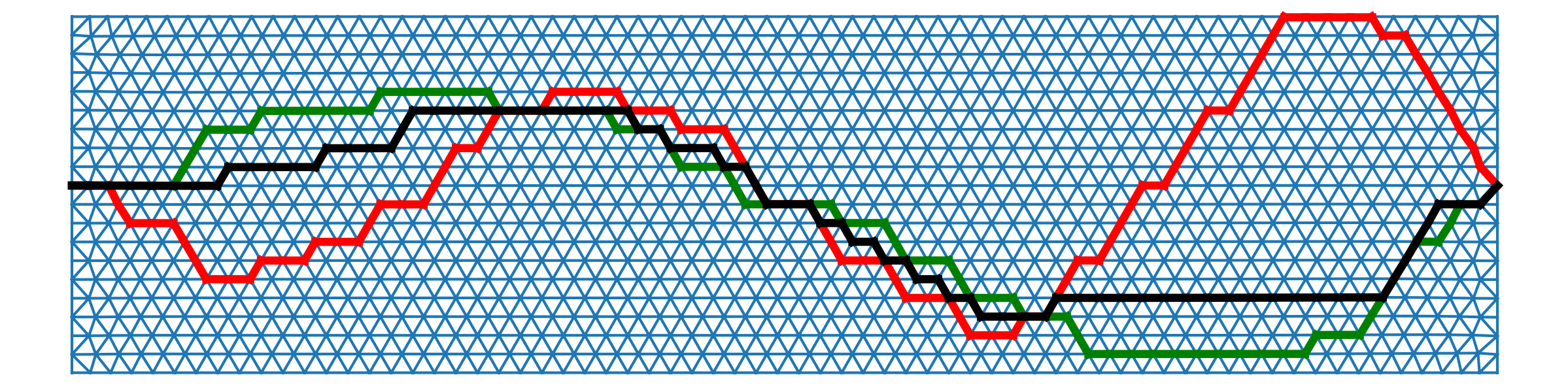
Figure 25: Simplicial median shape of two curves in 2D. The input curves are shown in green and red, while the median shape curve is shown in black.

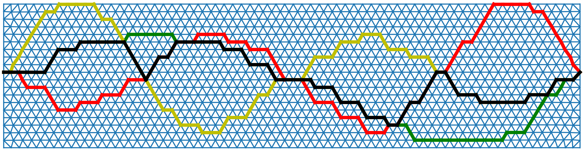
Figure 26: Simplicial median shape of three curves in 2D. The third input curve in yellow is added to the two in green and red, which are the input curves in Figure 25. The median shape curve is shown in black.

7.2 Instances in 3D

We present instances with codimensions $1$ and $2$ in $\mathbb{R}^{3}$. In all these instances, the input currents had shared boundaries. We constructed a $3$-complex tetrahedralizing a $3$-ball, consisting of $45,768$ tetrahedra. The $2$-skeleton of this complex had $93,149$ triangles and $55,860$ edges. We considered three input curves, each of which went from the North pole to the South pole, meeting roughly at $120$ degree angles at both poles. We started with the curves living on the surface, i.e., on the $2$-sphere, and added some noise so that they wiggled into the interior of the $3$-ball at places. One would expect the median shape to be the diameter connecting the North and south poles, and our computations agreed with this intuition.

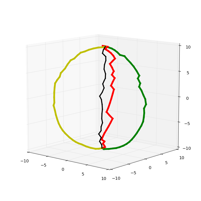
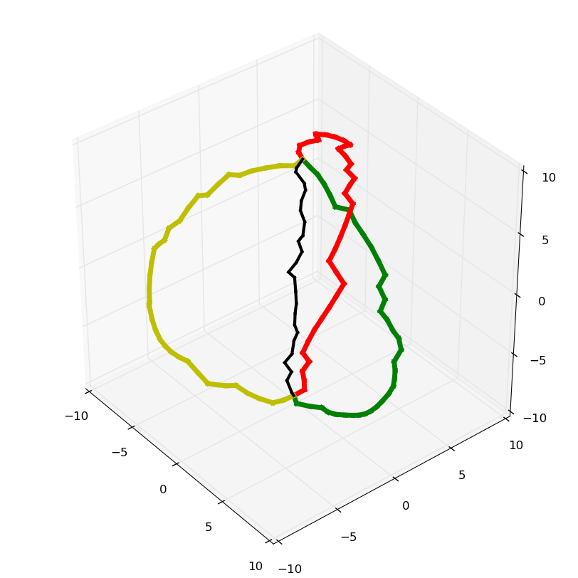
Figure 27: Tow views of the simplicial median shape of three curves in a $3$-ball in $\mathbb{R}^{3}$. The input curves are shown in green, red, and yellow, while the median shape curve is shown in black.

We next considered two similar input curves (between the poles), and solved the generalized weighted simplicial median shape problem over the $2$-sphere, i.e., the surface of the $3$-ball. The $2$-complex triangulating the $2$-sphere had $8,695$ edges and $5,788$ triangles. As we vary the weights $[\alpha_{1}~{}\alpha_{2}]$ from $[1~{}~{}0]$ to $[0~{}~{}1]$, the median shape changes from the first to the second input curve, all along the surface of the sphere (see Figure 28).

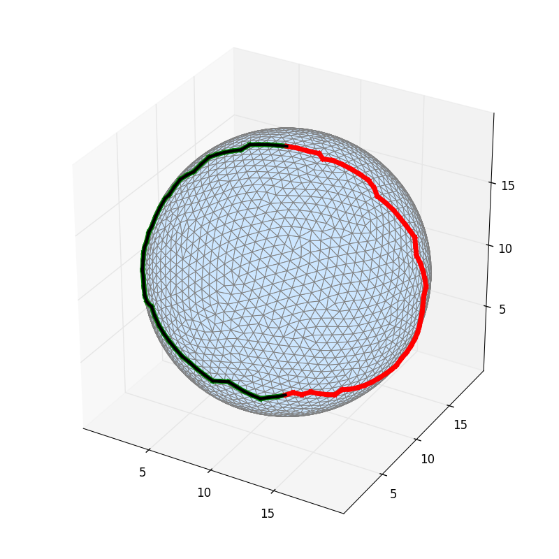
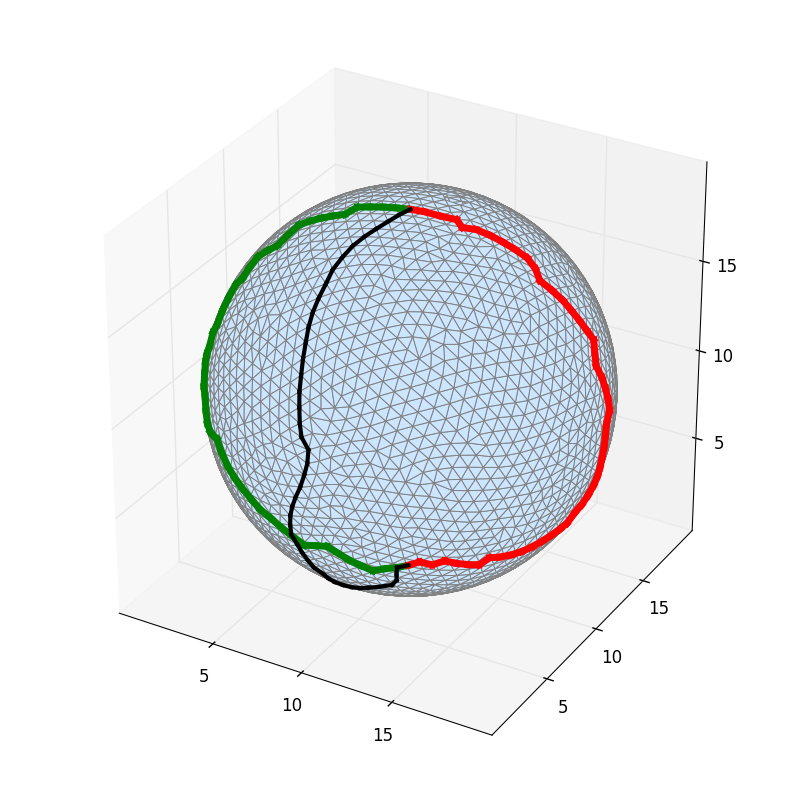
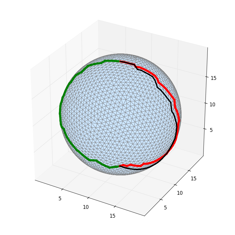
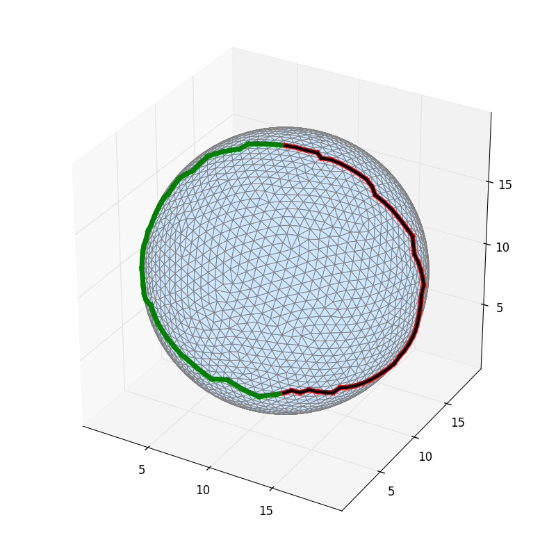
Figure 28: Weighted median shape of $2$ pole-to-pole curves on a $2$-sphere. The input curves are shown in green and red, while the median shape curve is shown in black. The weights $[\alpha_{!}~{}\alpha_{2}]$ for the two input curves were chosen as $[1~{}0]$ in the top left figure and $[0~{}1]$ in the bottom right figure. The weights are $[0.5~{}0.5]$ in the top right figure and $[0.1,0.9]$ in the bottom left figure.

To further demonstrate the versatility of simplicial flat norm (as described in Section 6.3.1), we present computations on a torus in Figure 29. The triangulation of the torus had $5,007$ edges and $3,336$ triangles. We consider two cases each with a pair of input currents—a pair of handle loops and another pair of tunnel loops.

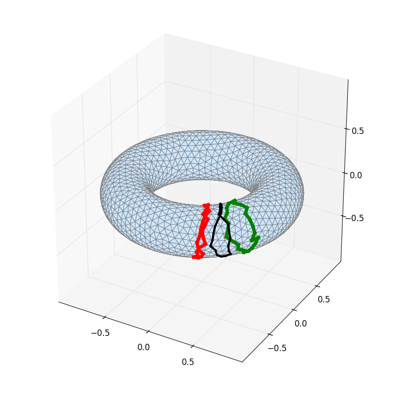
Figure 29: Simplicial median shapes of two tunnel curves and two handle curves on a torus. The input curves are shown in green and red, while the median shape curve is shown in black.

It is worth noting that the boundary matrix in question ($[\partial_{2}]$) is not totally unimodular in the case of the $3$-ball (for computations shown in Figure 27). On the other hand, the boundary matrix of the $2$-sphere as well as the torus are indeed totally unimodular (for computations shown in Figure 28 and Figure 29). At the same time, the constraint matrix of the LPs in all these cases need not be totally unimodular even if the boundary matrix is totally unimodular.

We have also worked with instances of surfaces in $\mathbb{R}^{3}$ (i.e., codimension $1$ in 3D). One such instance is made available as part of our open source software repository available at
https://github.com/tbtraltaa/medianshape.

8 Discussion

8.1 Theory

The theory we have presented in the first four sections of this paper is just a beginning. We list a few of the directions inviting further work:

Big $\lambda$:

We have explored the codimension 1 case of the median problem fairly thoroughly, though the study of that problem for $\lambda$ that is not small, remains. (By small $\lambda$, we mean $\lambda$ small enough to guarantee that for each $i$, the multiscale flat norm of $\hat{T}-\operatorname{T}_{i}$ equals the mass of $S_{i}$ where $\partial S_{i}=(\hat{T}-\operatorname{T}_{i})$.)

Non-shared Boundaries:

The case of codimension 1 input currents that do not share boundaries is completely open. It seems that there is a sort of soft transition from shared boundaries to non-shared boundaries that could be studied first. By this we mean input currents that almost share boundaries in the sense that the Hausdorff distance between the supports of the boundaries of all the input currents is much smaller than the diameter of any of supports the input currents, which in turn are comparable to the diameter of the supports of the boundaries. In other words, first study the case in which:

1. Boundaries are close: $\operatorname{H}(\operatorname{supp}(\partial T_{i}),\operatorname{supp}(\partial T_{j}))\leq\delta$ for all $i$ and $j$

2. we have $\delta<<\operatorname{diam}(\operatorname{supp}(T_{i}))$ for all $i$,

3. and $\operatorname{diam}(\operatorname{supp}(T_{i}))\approx\operatorname{diam}(\operatorname{supp}(\partial T_{i}))$ for all $i$.

where $\operatorname{H}(E,F)$ is the Hausdorff distance between the sets $E$ and $F$.

Higher Codimension:

We just scratched the surface of the case of input currents with higher codimension. In general higher codimension increases the difficulty of studies—see for example the technicalities in the study of the regularity of minimizing currents in higher codimension by Almgren [2], which were recently illuminated by the work of De Lellis and Spodaro, which by itself is still impressively large; see De Lellis’ overview here [15] as well as [16, 17, 18, 22]. See also the work they did with Spolaor here [19, 20, 21].

Means:

We left the entire subject of flat norm based means open, due to the difficulty in computing the means. It is also the case that the medians seem a bit more natural geometrically. On the other hand, means are closer to unique and their study would almost certainly raise interesting theoretical questions

Interpolation:

What sorts of paths in the space of currents would be traversed if we introduced time evolving $\lambda_{i(t)}$’s for each $T_{i}$ so that the resulting objective function becomes $\sum_{i=1}^{N}\mathbb{F}_{\lambda_{i(t)}}(T-T_{i})$? How we can smoothly interpolate between shapes is of practical interest if the computation of those paths could be made tractable.

8.2 Computation

It is rather surprising that we are obtaining integer optimal solutions for the median shape LPs even when the constraint matrices are not guaranteed to be totally unimodular. Could we characterize the classes of simplicial complexes for which this property holds? Previously, we had presented a class of simplicial complexes that are non total-unimodularity neutralized [40], on which instances of the optimal homologous chain problem (OHCP) linear program are guaranteed to have integer optimal solutions even when the boundary matrix is not totally unimodular. At the same time, this characterization depended critically on the coefficients of the $(p+1)$-dimensional simplices, e.g., triangles in the edge-triangle case, being all zero in the objective function. We do not have this condition satisfied in the simplicial flat norm LP or in the median shape LP.

While we are able to solve the simplicial median shape problem as a linear program, the LPs themselves could be quite large in size, and take a long time to solve in practice. For instance, the median shape LPs in the $3$-ball examples (shown in Figure 27) had more than a million columns ($1,005,774$ to be exact). Could we design an algorithm that solves the median shape LP much faster than general LPs, the most efficient algorithms for which take time that grows as the cube of the number of columns?

References

- [1] Ravindra K. Ahuja, Thomas L. Magnanti, and James B. Orlin. Network Flows: Theory, Algorithms, and Applications. Pearson, 1993.
- [2] Frederick J. Almgren, Jr. Almgren’s big regularity paper, volume 1 of World Scientific Monograph Series in Mathematics. World Scientific Publishing Co. Inc., River Edge, NJ, 2000. -valued functions minimizing Dirichlet’s integral and the regularity of area-minimizing rectifiable currents up to codimension 2, With a preface by Jean E. Taylor and Vladimir Scheffer.
- [3] Djamila Aouada. Geometric, Statistical, and Topological Modeling of Intrinsic Data Manifolds: Application to Three-dimensional Shapes. ProQuest, 2009.
- [4] Djamila Aouada and Hamid Krim. Squigraphs for fine and compact modeling of 3-d shapes. Image Processing, IEEE Transactions on, 19(2):306–321, 2010.
- [5] M Faisal Beg, Michael I Miller, Alain Trouvé, and Laurent Younes. Computing large deformation metric mappings via geodesic flows of diffeomorphisms. International journal of computer vision, 61(2):139–157, 2005.
- [6] Benjamin Berkels, Gina Linkmann, and Martin Rumpf. An SL(2) invariant shape median. Journal of Mathematical Imaging and Vision, 37(2):85–97, 2010.
- [7] Dimitris Bertsimas and John N. Tsitsiklis. Introduction to Linear Optimization. Athena Scientific, Belmont, MA., 1997.
- [8] Nicolas Charon. Analysis of geometric and functional shapes with extensions of currents: applications to registration and atlas estimation. PhD thesis, École normale supérieure de Cachan-ENS Cachan, 2013.
- [9] Nicolas Charon and Alain Trouvé. The varifold representation of nonoriented shapes for diffeomorphic registration. SIAM Journal on Imaging Sciences, 6(4):2547–2580, 2013.
- [10] Nicolas Charon and Alain Trouvé. Functional currents: a new mathematical tool to model and analyse functional shapes. Journal of mathematical imaging and vision, 48(3):413–431, 2014.
- [11] Guillaume Charpiat, Olivier Faugeras, Renaud Keriven, and Pierre Maurel. Distance-based shape statistics. In Acoustics, Speech and Signal Processing, 2006. ICASSP 2006 Proceedings. 2006 IEEE International Conference on, volume 5, pages V–V. IEEE, 2006.
- [12] Gérard Cornuéjols. Combinatorial Optimization: Packing and Covering. Society for Industrial and Applied Mathematics, Philadelphia, PA, USA, 2001.
- [13] IBM ILOG CPLEX Optimizer, Version 12.6.1. http://www-01.ibm.com/software/integration/optimization/cplex-optimizer, 2015.
- [14] Daniel Cremers, Timo Kohlberger, and Christoph Schnörr. Shape statistics in kernel space for variational image segmentation. Pattern Recognition, 36(9):1929–1943, 2003.
- [15] Camillo De Lellis. Almgren’s q-valued functions revisited. In Proceedings of the International Congress of Mathematicians 2010 (ICM 2010) (In 4 Volumes) Vol. I: Plenary Lectures and Ceremonies Vols. II–IV: Invited Lectures, pages 1910–1933. World Scientific, 2010.
- [16] Camillo De Lellis and Emanuele Spadaro. Regularity of area minimizing currents II: center manifold. arXiv preprint arXiv:1306.1191, 2013.
- [17] Camillo De Lellis and Emanuele Spadaro. Regularity of area minimizing currents III: blow-up. arXiv preprint arXiv:1306.1194, 2013.
- [18] Camillo De Lellis and Emanuele Spadaro. Regularity of area minimizing currents I: gradient estimates. Geometric and Functional Analysis, 24(6):1831–1884, 2014.
- [19] Camillo De Lellis, Emanuele Spadaro, and Luca Spolaor. Regularity theory for -dimensional almost minimal currents iii: blowup. arXiv preprint arXiv:1508.05510, 2015.
- [20] Camillo De Lellis, Emanuele Spadaro, and Luca Spolaor. Regularity theory for 2-dimensional almost minimal currents ii: branched center manifold. Annals of PDE, 3(2):18, 2017.
- [21] Camillo De Lellis, Emanuele Spadaro, and Luca Spolaor. Regularity theory for 2-dimensional almost minimal currents i: Lipschitz approximation. Transactions of the American Mathematical Society, 370(3):1783–1801, 2018.
- [22] Camillo De Lellis and Emanuele Nunzio Spadaro. Q-valued functions revisited. American Mathematical Soc., 2011.
- [23] Tamal K. Dey, Anil N. Hirani, and Bala Krishnamoorthy. Optimal homologous cycles, total unimodularity, and linear programming. SIAM Journal on Computing, 40(4):1026–1040, 2011. arxiv:1001.0338.
- [24] Nathan M. Dunfield and Anil N. Hirani. The least spanning area of a knot and the optimal bounding chain problem. In Prooceedings of the 27th ACM Annual Symposium on Computational Geometry, SoCG ’11, pages 135–144, 2011.
- [25] Lawrence C. Evans and Ronald F. Gariepy. Measure Theory and Fine Properties of Functions. Studies in Advanced Mathematics. CRC Press, 1992. ISBN 0-8493-7157-0.
- [26] Lawrence C Evans and Ronald F Gariepy. Measure Theory and Fine Properties of Functions, volume 5. CRC press, revised edition, 2015.
- [27] Herbert Federer. Geometric Measure Theory.-Reprint of the 1969 Edition. Springer, 1996.
- [28] J. Glaunès and S. Joshi. Template estimation form unlabeled point set data and surfaces for computational anatomy. JMIV, 2007. Proceedings of Mathematical Foundations of Computational Anatomy, MICCAI 2006.
- [29] Joan Glaunès. Transport par difféomorphismes de points, de mesures et de courants pour la comparaison de formes et l’ anatomie numérique. PhD thesis, l’ Université Paris 13 en Mathématiques, 2005.
- [30] Colin Goodall. Procrustes methods in the statistical analysis of shape. Journal of the Royal Statistical Society. Series B (Methodological), pages 285–339, 1991.
- [31] Steven Haker, Lei Zhu, Allen Tannenbaum, and Sigurd Angenent. Optimal mass transport for registration and warping. International Journal of computer vision, 60(3):225–240, 2004.
- [32] Frank Harary. Graph Theory. Addison-Wesley, 1969.
- [33] Sharif Ibrahim, Bala Krishnamoorthy, and Kevin Vixie. Flat norm decomposition of integral currents. Journal of Computational Geometry, 7(1):285–307, 2016. http://arxiv.org/abs/1411.0882.
- [34] Sharif Ibrahim, Bala Krishnamoorthy, and Kevin R. Vixie. Simplicial flat norm with scale. Journal of Computational Geometry, 4(1):133–159, 2013. arXiv:1105.5104.
- [35] Sharif Ibrahim, Bala Krishnamoorthy, and Kevin R. Vixie. Flat norm decomposition of integral currents. Journal of Computational Geometry, 7(1):285–307, 2016. arXiv:1411.0882.
- [36] Iréne Kaltenmark. Geometrical Growth Models for Computational Anatomy. PhD thesis, Université Paris-Saclay, 2016.
- [37] DG Kendall. The statistics of shape. Interpreting multivariate data, pages 75–80, 1981.
- [38] Steven G. Krantz and Harold R. Parks. Geometric Integration Theory. Birkhauser, 2008. ISBN-13: 978-0-8176-4676-9.
- [39] Hamid Krim and Anthony J Yezzi. Statistics and analysis of shapes. Springer, 2006.
- [40] Bala Krishnamoorthy and Gavin W. Smith. Non total-unimodularity neutralized simplicial complexes. Discrete Applied Mathematics, 2016. arxiv:1304.4985.
- [41] Brian Krummel. Regularity of minimal hypersurfaces with a common free boundary. Calculus of Variations and Partial Differential Equations, 8(3):525– 537, Nov 2014.
- [42] Fang-Hua Lin and Xiaoping Yang. Geometric measure theory: an introduction. Science Press, 2002.
- [43] Francesco Maggi. Sets of finite perimeter and geometric variational problems: an introduction to Geometric Measure Theory. Cambridge University Press, 2012.
- [44] Pertti Mattila. Geometry of sets and measures in Euclidean spaces: fractals and rectifiability, volume 44. Cambridge University Press, 1999.
- [45] Frank Morgan. Geometric measure theory: a beginner’s guide. Academic Press, fourth edition, 2008.
- [46] Simon P. Morgan and Kevin R. Vixie. TV computes the flat norm for boundaries. Abstract and Applied Analysis, 2007:Article ID 45153, 14 pages, 2007. doi:10.1155/2007/45153.
- [47] James G. Oxley. Matroid Theory. Oxford University Press, Inc., New York, NY, USA, 2 edition, 2006.
- [48] F James Rohlf. Shape statistics: Procrustes superimpositions and tangent spaces. Journal of Classification, 16(2):197–223, 1999.
- [49] Martin Rumpf and Benedikt Wirth. Variational methods in shape analysis. In Handbook of Mathematical Methods in Imaging, pages 1363–1401. Springer, 2011.
- [50] Alexander Schrijver. Theory of Linear and Integer Programming. Wiley-Interscience Series in Discrete Mathematics. John Wiley & Sons Ltd., Chichester, 1986.
- [51] Leon Simon. Lectures On Geometric Measure Theory. Proceedings Of The Centre For Mathematical Analysis, Australian National University, 1984.
- [52] Klaus Truemper. Matroid Decomposition. Academic Press Inc., Boston, MA, 1992.
- [53] Marc Vaillant and Joan Glaunès. Surface matching via currents. In Proceedings of Information Processing in Medical Imaging (IPMI 2005), volume 3565 of Lecture Notes in Computer Science. Springer, 2005.
- [54] Kevin R. Vixie, Keith Clawson, Thomas J. Asaki, Gary Sandine, Simon P. Morgan, and Brandon Price. Multiscale flat norm signatures for shapes and images. Applied Mathematical Sciences, 4(14):667–680, 2010.
- [55] Hassler Whitney. Geometric Integration Theory. Princeton University Press, 1957.