A Posteriori Error Estimate for Computing $\operatorname{tr}(f(A))$ by Using the Lanczos Method

Abstract

An outstanding problem when computing a function of a matrix, $f(A)$, by using a Krylov method is to accurately estimate errors when convergence is slow. Apart from the case of the exponential function which has been extensively studied in the past, there are no well-established solutions to the problem. Often the quantity of interest in applications is not the matrix $f(A)$ itself, but rather, matrix-vector products or bilinear forms. When the computation related to $f(A)$ is a building block of a larger problem (e.g., approximately computing its trace), a consequence of the lack of reliable error estimates is that the accuracy of the computed result is unknown. In this paper, we consider the problem of computing $\operatorname{tr}(f(A))$ for a symmetric positive-definite matrix $A$ by using the Lanczos method and make two contributions: (i) we propose an error estimate for the bilinear form associated with $f(A)$, and (ii) an error estimate for the trace of $f(A)$. We demonstrate the practical usefulness of these estimates for large matrices and in particular, show that the trace error estimate is indicative of the number of accurate digits. As an application, we compute the log-determinant of a covariance matrix in Gaussian process analysis and underline the importance of error tolerance as a stopping criterion, as a means of bounding the number of Lanczos steps to achieve a desired accuracy.

keywords

Matrix trace, matrix function, Lanczos method, error estimate, confidence interval

1 Introduction

The trace of a function of a matrix, $\operatorname{tr}(f(A))$, occurs in diverse areas including scientific computing, statistics, and machine learning [3, 19, 35, 11, 29, 4, 1, 36, 34, 23, 40, 27]. Often in applications, the matrix $A$ is so large that explicitly forming $f(A)$ is not a practically viable option. In this work, we focus on the case when $A\in^{n\times n}$ is symmetric positive-definite, so that it admits a spectral decomposition $Q^{T}AQ=\operatorname{diag}(\lambda_{1},\ldots,\lambda_{n})$, where the $\lambda_{i}$’s are real positive eigenvalues and $Q$ is the matrix of normalized eigenvectors. Naturally, $f$ must be (at least) defined on the spectrum of $A$, although for analysis, we will assume that $f$ is analytic inside some contour enclosing the spectrum. Then, $\operatorname{tr}(f(A))$ is nothing but the sum of the $f(\lambda_{i})$’s. Computing the trace in this manner, however, requires the computation of all the eigenvalues, which is also often prohibitively expensive. Hence, various methods proposed for approximately computing $\operatorname{tr}(f(A))$ consist of the following two ingredients [17, 24, 3, 2, 23, 26, 22, 13, 14].

1. Approximate the trace of $f(A)$ by using the average of unbiased samples $u_{i}^{T}f(A)u_{i}$, $i=1,\ldots,N$, where the $u_{i}$’s are independent random vectors of some nature.

2. Approximately compute the bilinear form $u_{i}^{T}f(A)u_{i}$ by using some numerical technique.

The various methods differ in the random mechanism of selecting the $u_{i}$’s and the numerical technique for computing the bilinear form. Several variants of these ingredients exist (e.g., computing deterministically $\operatorname{tr}(f(A))=\sum_{i=1}^{n}e_{i}^{T}f(A)e_{i}$ rather than using random vectors $u_{i}$, or even using block vectors to replace the canonical vectors $e_{i}$ [5]; or using moment extrapolation for particularly $f(t)=t^{\alpha}$ with real value $\alpha$ [28, 6]), but they are not the focus of this work. In the two ingredients, the convergence of the approximation is generally gauged through a combination of Monte Carlo convergence of the sample average and the convergence of the numerical technique. In practice, however, the convergence results obtained for these methods [2, 39, 30, 23, 22] rarely translate into practical schemes to monitor convergence. Monitoring the accuracy of a given approximation to $\operatorname{tr}(f(A))$ can be very challenging for certain functions $f$. This is in complete contrast to the situation prevalent when solving linear systems, where simple residual norms provide a computable measure of the backward error. The practical question we woud like to address is given the number $N$ of random vectors and a stopping criterion for the bilinear form, how accurate is the computed result?

The idea is to obtain tight a-posteriori error estimates for both of the ingredients mentioned above and then to combine these estimates. For the sample average, we will establish confidence intervals. The computed approximation (a point estimate in a statistics language) to $\operatorname{tr}(f(A))$ alone does not carry any information on accuracy; however, combined with a confidence interval (an interval estimate), it gives a notion of absolute/relative error with (high) probability. The difference with standard statistics, on the other hand, is that each sample itself bears a numerical error. Hence, for the approximation of the bilinear form, we impose a stopping criterion—error tolerance $\delta$—and inject $\delta$ into the confidence interval. The confidence interval thus indicates that with a certain (high) probability, the trace approximation error is bounded by some expression in terms of $N$ and $\delta$. As we will demonstrate in experiments, this bound is generally indicative of the number of accurate digits.

Then, monitoring the error in the approximation of the bilinear form is crucial for an accurate understanding of the overall error in the trace. The monitoring mechanism must depend on the approximation method used. In this work we focus on the Lanczos method, which has many appealing properties and which has long been a preferred technique for approximating full or partial spectra of large symmetric matrices, through inexpensive matrix-vector multiplications. An outstanding problem, however, is that good extensions of the a-posteriori error estimate given in Saad [31] to more general functions than the exponential are rare. The Lanczos method can be considered a polynomial approximation technique, where $f$ is approximated by a polynomial that interpolates $f$ on the Ritz values, but it typically converges twice as fast as other polynomial approximation methods (e.g., Chebyshev approximation) [37, Chapter 19]. Such a faster convergence is owed to the Gauss-quadrature interpretation that will be discussed shortly.

Let us briefly review the Lanczos method. It begins with a unit vector $v_{1}$ and coefficient $\beta_{1}=0$ and computes the sequence of vectors

$$v_{k+1}=(Av_{k}-\alpha_{k}v_{k}-\beta_{k}v_{k-1})/\beta_{k+1},\quad\text{for }k=1,2,\ldots,$$ (1)

where $\alpha_{k}=v_{k}^{T}Av_{k}$, and $\beta_{k+1}$ is a normalization factor such that $v_{k+1}$ has a unit norm. After $m$ steps, the above iteration results in the matrix identity

$$AV_{m}=V_{m}T_{m}+\beta_{m+1}v_{m+1}e_{m}^{T},$$ (2)

where

$$V_{m}=[v_{1},v_{2},\ldots,v_{m}]\quad\text{and}\quad T_{m}=\begin{bmatrix}\alpha_{1}&\beta_{2}\\ \beta_{2}&\alpha_{2}&\beta_{3}\\ &\beta_{3}&\alpha_{3}&\ddots\\ &&\ddots&\ddots&\beta_{m}\\ &&&\beta_{m}&\alpha_{m}\end{bmatrix}.$$

In exact arithmetic, the columns of $V_{m}$, together with $v_{m+1}$, consist of an orthonormal basis of the Krylov subspace $\operatorname{span}\{v_{1},Av_{1},\ldots,A^{m-1}v_{1},A^{m}v_{1}\}$, and the symmetric tridiagonal matrix $T_{m}$ is sometimes called the Jacobi matrix. Then, omitting the index $i$ in the random vector $u_{i}$ for clarity, the Lanczos method approximates the bilinear form $u^{T}f(A)u$ through a projection on the Krylov subspace; i.e., $u^{T}V_{m}f(V_{m}^{T}AV_{m})V_{m}^{T}u$. If the starting Lanczos vector $v_{1}$ is a normalized $u$, then this quantity is simply $\|u\|^{2}e_{1}^{T}f(T_{m})e_{1}$.

The same approximate quantity may be derived from a different viewpoint. Based on the spectral decomposition of $A$, one may write

$$u^{T}f(A)u=\sum_{i=1}^{n}f(\lambda_{i}){\omega_{i}^{2}=\int f(\lambda)\,d\omega}(\lambda),$$ (3)

where the $\omega_{i}$’s are elements of the vector $Q^{T}u$, $\omega(\lambda)$ is a discrete measure with masses $\omega_{i}^{2}$ at the atoms $\lambda_{i}$, and the integral is a Stieltjes integral. One may show [32, 18] that there is a sequence of polynomials $p_{k}(\lambda)$ associated with this process satisfying the relation $v_{k}=p_{k-1}(A)v_{1}$, $k=1,2,\ldots,m$, that are orthonormal with respect to the measure $\omega(\lambda)$. Then, applying the Golub–Welsch algorithm [20], the Gauss quadrature rule for the integral (3) uses the eigenvalues of $T_{m}$ as the quadrature points, and the square of the first element of the normalized eigenvectors of $T_{m}$, multiplied by $\int d\omega=\|u\|^{2}$, as the quadrature weights. In other words, writing the spectral decomposition $S^{T}T_{m}S=\Theta$, the quadrature rule gives

$$\int f(\lambda)\,d\omega(\lambda)\approx\sum_{k=1}^{m}\underbrace{\|u\|^{2}S_{1k}^{2}}_{\text{weights}}f(\underbrace{\Theta_{kk}}_{\text{points}}),$$

which coincides with $\|u\|^{2}e_{1}^{T}f(T_{m})e_{1}$.

The quadrature interpretation is particularly useful for establishing exponential convergence of the Lanczos method, if $f$ admits certain analytic properties (see, e.g., Trefethen[37]). Interestingly, other related quadrature rules, in a combined use, may also yield bounds [18]. For example, if the even derivatives of $f$ in the spectrum interval have a constant sign, then the Gauss rule and the Gauss–Lobatto rule always give results on the two sides of $u^{T}f(A)u$. Similarly, if the odd derivatives of $f$ have a constant sign, then the two results of the Gauss–Radau rule always straddle around the bilinear form. Moreover, bounds for the particular case when $f$ is a rational function were also proposed [16, 15], based on similar ideas of Gauss and Gauss-related quadratures. In practice, however, these bounds are often too conservative as an error estimate, especially when convergence is slow. Thus, a contribution of this work is a more accurate error estimate of the approximation $\|u\|^{2}e_{1}^{T}f(T_{m})e_{1}$ to $u^{T}f(A)u$. This estimate is directly used to check against the aforementioned tolerance $\delta$ for monitoring progress.

It is noteworthy to relate this work with a prior work [9] by the first author, who studied the trace error by using a similar approach, and to underline a distinction between the two contributions. Both works consider the combination of statistical error caused by sample average and the numerical error in evaluating the bilinear form $u^{T}f(A)u$. In quantifying the statistical error, the prior work exploited a variance term defined through an estimator, which is applicable only to random Gaussian vectors. In this work, the variance is the sample variance (albeit carrying numerical error) and thus there is no restriction on the random mechanism of the random vectors. This distinction has a consequence on the handling of numerical error. In order to establish a confidence interval, the previous work proposed a stopping criterion for the approximation of the function $f$ such that the numerical error is comparable with the statistical error. On the other hand, in this work, we allow any tolerance $\delta$ for the approximation of the bilinear form $u^{T}f(A)u$, because $\delta$ is written into the confidence interval. Of course, one may find an appropriate $\delta$ that makes the two sources of errors comparable, in a post-hoc manner, but this benefit comes only as a by-product. Nevertheless, the post-hoc adjustment of $\delta$ is practically useful; see the next section.

2 Confidence interval with numerical error

To establish a confidence interval that incorporates numerical errors in the samples, let us first define some notation. Denote by

1. $\mu:=\operatorname{tr}(f(A))$, the mean;

2. $x_{i}:=u_{i}^{T}f(A)u_{i}$, an independent, unbiased sample; and

3. $x_{i}^{(m)}:=\|u_{i}\|^{2}e_{1}^{T}f(T_{m}^{(i)})e_{1}$, a sample with numerical error,

where we have added a superscript $(i)$ to the Jacobi matrix to distinguish different samples. Formally, the trace approximation method considered in this work refers to approximating the mean $\mu$ by using the sample average

$$\bar{x}^{(m)}:=\frac{1}{N}\sum_{i=1}^{N}x_{i}^{(m)}.$$

The corresponding sample standard error is

$$s^{(m)}:=\sqrt{\frac{1}{N-1}\sum_{i=1}^{N}\left(x_{i}^{(m)}-\bar{x}^{(m)}\right)^{2}}.$$

In standard statistics, one may establish confidence intervals for only the average of the samples without numerical error/bias:

$$\bar{x}:=\frac{1}{N}\sum_{i=1}^{N}x_{i}.$$

Hence, defining the standard error

$$s:=\sqrt{\frac{1}{N-1}\sum_{i=1}^{N}(x_{i}-\bar{x})^{2}},$$

for any $\alpha>0$, we let

$$p_{\alpha}:=\operatorname{Pr}\left(|\bar{x}-\mu|\leq\frac{\alpha s}{\sqrt{N}}\right).$$ (4)

The parameter $\alpha$ is to be interpreted as a “multiple of the standard error,” and the associated probability $p_{\alpha}$ is one minus the significance level. When $N$ is sufficiently large (e.g., $N\geq 30$), by the central limit theorem, the standardized error $\sqrt{N}|\bar{x}-\mu|/s$ approximately follows the standard normal distribution. Hence, $p_{\alpha}$ is approximately the probability of a Gaussian sample whose absolute value is no greater than $\alpha$, i.e.,

$$p_{\alpha}\approx\operatorname{erf}(\alpha/\sqrt{2}),$$

where $\operatorname{erf}$ is the error function.

The main result of this section is a probability estimate resembling (4), for the sample average $\bar{x}^{(m)}$ with numerical error.

Theorem 1.

Suppose the sample bias is bounded by some $\delta>0$; that is, $|x_{i}-x_{i}^{(m)}|\leq\delta$ for all $i$, then

$$\operatorname{Pr}\left\{|\bar{x}^{(m)}-\mu|\leq\frac{\alpha}{\sqrt{N}}\left(s^{(m)}+\delta\sqrt{\frac{N}{N-1}}\right)+\delta\right\}\geq p_{\alpha}.$$

Proof.

Let $x_{i}-x_{i}^{(m)}=\delta_{i}$ and $\bar{x}-\bar{x}^{(m)}=\bar{\delta}$. Form a vector $a$ with elements $x_{i}^{(m)}-\bar{x}^{(m)}$ and another vector $b$ with elements $\delta_{i}-\bar{\delta}$. Note that $a+b$ consists of elements $x_{i}-\bar{x}$. Then, the triangle inequality $\|a+b\|\leq\|a\|+\|b\|$ translates to

$$s\sqrt{N-1}\leq s^{(m)}\sqrt{N-1}+\sqrt{\sum_{i=1}^{N}\left(\delta_{i}-\bar{\delta}\right)^{2}}.$$

Because $|\delta_{i}|\leq\delta$, we have

$$\sum_{i=1}^{N}\left(\delta_{i}-\bar{\delta}\right)^{2}=\sum_{i=1}^{N}\delta_{i}^{2}-N\bar{\delta}^{2}\leq N\delta^{2}-N\bar{\delta}^{2}\leq N\delta^{2}.$$

Hence,

$$s\leq s^{(m)}+\delta\sqrt{\frac{N}{N-1}}.$$

Therefore, based on (4), we have that with probability greater than $p_{\alpha}$,

$$|\bar{x}^{(m)}-\mu|\leq|\bar{x}-\mu|+|\bar{x}-\bar{x}^{(m)}|\leq\frac{\alpha s}{\sqrt{N}}+|\bar{\delta}|\leq\frac{\alpha}{\sqrt{N}}\left(s^{(m)}+\delta\sqrt{\frac{N}{N-1}}\right)+\delta,$$

which concludes the proof. ∎

Theorem 1 gives a computable bound. For any reasonable $\alpha$ (e.g., $3$, which translates to a probability $p_{\alpha}\approx 99.73\%$), the error of the sample average $\bar{x}^{(m)}$ is bounded by an expression that involves only the number $N$ of samples, the error tolerance $\delta$, and the standard error $s^{(m)}$. In later experiments, we will use this bound to assess the quality of approximation and show that it is indicative of the true error.

One may be interested in an appropriate $\delta$ that makes the numerical error comparable with the statistical one. A natural idea is to let the tolerance $\delta$ be approximately the statistical error bound $\alpha s^{(m)}/\sqrt{N}$, or $\beta\alpha s^{(m)}/\sqrt{N}$ for some small $\beta$ (e.g., $0.1$). The following result gives a straightforward bound that bypasses the reliance on $\delta$ for such a case; the overall error increases to approximately $(1+\beta)\alpha s^{(m)}/\sqrt{N}$. This result may be used to adjust the tolerance $\delta$ given the standard error $s^{(m)}$ obtained in a previous calculation.

Corollary 2.

Under the conditions of Theorem 1, for any $\beta>0$, if $\delta\leq\beta\alpha s^{(m)}/\sqrt{N}$, then

$$\operatorname{Pr}\left\{|\bar{x}^{(m)}-\mu|\leq\frac{\alpha s^{(m)}}{\sqrt{N}}\left(1+\beta+\frac{\beta\alpha}{\sqrt{N-1}}\right)\right\}\geq p_{\alpha}.$$

Proof.

Clearly, if $\delta$ satisfies the stated condition, then

$$\frac{\alpha}{\sqrt{N}}\left(s^{(m)}+\delta\sqrt{\frac{N}{N-1}}\right)+\delta\leq\frac{\alpha s^{(m)}}{\sqrt{N}}\left(1+\beta+\frac{\beta\alpha}{\sqrt{N-1}}\right).$$

The proof ends by noting that enlarging an upper bound increases the probability. ∎

3 Error estimation of bilinear form

With the confidence interval established in Theorem 1, we now consider how to reliably estimate the difference between $u^{T}f(A)u$ and $\|u\|^{2}e_{1}^{T}f(T_{m})e_{1}$, because this error will be used to check against the tolerance $\delta$ for convergence. A challenge in computing matrix functions based on the Lanczos method is that good error estimates are hardly known, except for the simple case of the exponential [31] because of its fast convergence. Several error bounds were proposed [16, 15] but they are generally pessimistic and may deviate from the true error by one or more order of magnitudes, when convergence is slow. In this section, we propose a general technique applicable to a wide variety of functions and also to ill conditioned matrices.

3.1 Incremental and cumulative error

Omitting the common, known factor $\|u\|^{2}$, we define the quantity of interest

$$\rho_{m}:=v_{1}^{T}f(A)v_{1}-e_{1}^{T}f(T_{m})e_{1},$$

where recall that $v_{1}=u/\|u\|$. If the Lanczos iteration (1) is run to the end, we have

$$AV_{n}=V_{n}T_{n},$$ (5)

where the subscript $m$ in (2) is replaced by the matrix dimension $n$ and the remainder term vanishes. Therefore, $\rho_{m}$ is nothing but $e_{1}^{T}f(T_{n})e_{1}-e_{1}^{T}f(T_{m})e_{1}$.

We call $\rho_{m}$ the bilinear form error. In order to quantify this error, we define two additional terms closely related to $\rho_{m}$:

1. cumulative error: $d_{m,m^{\prime}}:=e_{1}^{T}f(T_{m^{\prime}})e_{1}-e_{1}^{T}f(T_{m})e_{1}$ for $m^{\prime}>m$;

2. incremental error: $d_{m}:=d_{m,m+1}$.

Clearly, the incremental error accounts for one step of the difference and the cumulative error accumulates the incremental errors for $m^{\prime}-m$ steps. In other words,

$$d_{m,m^{\prime}}=\sum_{i=m}^{m^{\prime}-1}d_{i}\quad\text{for all $m^{\prime}>m$ and particularly,}\quad\rho_{m}=d_{m,n}=\sum_{i=m}^{n-1}d_{i}.$$

3.2 Rational approximation

To estimate the bilinear form error $\rho_{m}$, we begin with the incremental error $d_{m}$, because it can be computed economically without evaluating $f(T_{m})$ for every $m$. The idea is to express $f$ with the Cauchy integral

$$f(a)=\frac{-1}{2\pi i}\int_{\Gamma}f(z)(a-z)^{-1}\,dz,$$

where $\Gamma$, inside which $f$ is analytic, is a contour enclosing $a$. Let the contour integral be approximated by using a quadrature rule

$$f(a)\approx\frac{-1}{2\pi i}\sum_{k=1}^{K}w_{k}f(z_{k})(a-z_{k})^{-1},$$

where $z_{k}$ and $w_{k}$ are the quadrature points and weights, respectively. Then, we effectively obtain a rational approximation of $f(a)$:

$$r_{K}(a)=\sum_{k=1}^{K}c_{k}(a-z_{k})^{-1},\quad\text{with}\quad c_{k}=\frac{-w_{k}f(z_{k})}{2\pi i},$$ (6)

where the poles $z_{k}$ are the same as the quadrature points and the coefficients $c_{k}$ are related to the quadrature weights $w_{k}$.

This intricate relationship between a rational approximation and a contour integral approximated by quadrature is well known. It is a valuable device for computing a function of a matrix times a vector, $f(A)b$, to high accuracy, because of the much faster convergence of rational approximations compared with polynomial approximations, provided that shifted linear systems with respect to $A$ are solved in a backward stable manner [21]. A challenge for applying this idea to large $A$ in practice, is that solving the systems by using a direct and stable method might not always be a viable option. Here, we will not discuss in detail the pros and cons of various methods for computing $f(A)b$, because the comparison is irrelevant. Instead, we use the device as a tool for analyzing $d_{m}=e_{1}^{T}f(T_{m+1})e_{1}-e_{1}^{T}f(T_{m})e_{1}$. An appealing consequence of the very fast convergence is that the number of quadrature points, $K$, need not be large to get sufficiently good approximations.

From a practical stand point, we refer the readers to articles [38, 21] and references therein for the rational approximations of a wide variety of functions used in applications (including, e.g., the exponential, the logarithm, and the square root). Some approximations are not written in the canonical form (6), but we will explain the simple modifications in later experiments. Moreover, because of conjugacy, and because we are interested in real arguments only, the number of summation terms in (6) may often be reduced by half. Therefore, throughout the paper we assume the following rational approximation:

$$r_{K}(x):=\operatorname{Re}\left\{\sum_{k=1}^{K}c_{k}(x-z_{k})^{-1}\right\},\quad x\in.$$ (7)

Because the spectrum interval of $T_{m}$ always stays inside that of $A$ (owing to the interlacing eigenvalue theorem), it suffices to use a contour that encloses the spectrum interval of $A$ so that the incremental error $d_{m}$ is well approximated by the following quantity:

$$d_{m}^{K} :=e_{1}^{T}r_{K}(T_{m+1})e_{1}-e_{1}^{T}r_{K}(T_{m})e_{1}$$

$$=\operatorname{Re}\left\{\sum_{k=1}^{K}c_{k}[e_{1}^{T}(T_{m+1}-z_{k}I)^{-1}e_{1}-e_{1}^{T}(T_{m}-z_{k}I)^{-1}e_{1}]\right\}.$$ (8)

The following result is in preparation for an iterative algorithm that efficiently computes $d_{m}^{K}$.

Proposition 3.

We have,

$$d_{m}^{K}=-\operatorname{Re}\left\{\sum_{k=1}^{K}c_{k}\beta_{m+1}[e_{m+1}^{T}(T_{m+1}-z_{k}I)^{-1}e_{1}][e_{m}^{T}(T_{m}-z_{k}I)^{-1}e_{1}]\right\},$$ (9)

where recall that $\beta_{m+1}$ is the last of the coefficients $\beta_{2}$, $\beta_{3}$, …in the Lanczos iteration (1).

Proof.

Note that $T_{m}-z_{k}I$ is a top-left block of $T_{m+1}-z_{k}I$. Thus, we are seeking the difference between the $(1,1)$ element of the inverse of a matrix and that of its top-left block. Recall the following identity:

$$\begin{bmatrix}R&S\\ T&U\end{bmatrix}^{-1}=\begin{bmatrix}R^{-1}+R^{-1}SQTR^{-1}&-R^{-1}SQ\\ -QTR^{-1}&Q\end{bmatrix},\quad\text{with}\quad Q=(U-TR^{-1}S)^{-1}.$$

It indicates that the difference between the $(1,1)$ element of $\left[\begin{smallmatrix}R&S\\ T&U\end{smallmatrix}\right]^{-1}$ and that of $R^{-1}$ is $e_{1}^{T}R^{-1}SQTR^{-1}e_{1}$.

In our setting, $\left[\begin{smallmatrix}R&S\\ T&U\end{smallmatrix}\right]=T_{m+1}-z_{k}I$ and $R=T_{m}-z_{k}I$. Therefore, $S=\beta_{m+1}e_{m}e_{1}^{T}$ and thus

$$e_{1}^{T}R^{-1}SQTR^{-1}e_{1}=\beta_{m+1}(e_{1}^{T}R^{-1}e_{m})(e_{1}^{T}QTR^{-1}e_{1}).$$

Clearly, $e_{1}^{T}R^{-1}e_{m}=e_{1}^{T}(T_{m}-z_{k}I)^{-1}e_{m}=e_{m}^{T}(T_{m}-z_{k}I)^{-1}e_{1}$ and $e_{1}^{T}QTR^{-1}e_{1}=-e_{m+1}^{T}(T_{m+1}-z_{k}I)^{-1}e_{1}$. Hence,

$$e_{1}^{T}(T_{m+1}-z_{k}I)^{-1}e_{1}-e_{1}^{T}(T_{m}-z_{k}I)^{-1}e_{1}=\\ -\beta_{m+1}[e_{m+1}^{T}(T_{m+1}-z_{k}I)^{-1}e_{1}][e_{m}^{T}(T_{m}-z_{k}I)^{-1}e_{1}],$$

which concludes the proof. ∎

For conciseness, in what follows, the three errors introduced in Section 3.1 may mean either the originally defined terms, or the approximated terms through rational approximation (7). This abuse of language will not cause confusion in the current context. The approximated terms have a superscript $K$ attached to the notation, just like $d_{m}^{K}$. The following result states that the error in the approximated terms is always bounded by two times the uniform error between $f$ and $r_{K}$.

Theorem 4.

Let $\|f-r_{K}\|_{\infty}:=\max_{x\in[\lambda_{\min},\lambda_{\max}]}|f(x)-r_{K}(x)|=\epsilon$, where $\lambda_{\min}$ and $\lambda_{\max}$ are the smallest and largest eigenvalues of $A$, respectively. For any $m$ and $m^{\prime}>m$ (including the case of incremental error $m^{\prime}=m+1$ and bilinear form error $m^{\prime}=n$), the cumulative error admits

$$|d_{m,m^{\prime}}-d_{m,m^{\prime}}^{K}|\leq 2\epsilon.$$

Proof.

Let the spectral decomposition of $T_{m}$ be $S\Theta S^{T}$. Then

$$|e_{1}^{T}f(T_{m})e_{1}-e_{1}^{T}r_{K}(T_{m})e_{1}|=|e_{1}^{T}S[f(\Theta)-r_{K}(\Theta)]S^{T}e_{1}|\leq\|f-r_{K}\|_{\infty}=\epsilon,$$

where the inequality comes from the fact that the vector $S^{T}e_{1}$ has a unit 2-norm. Since this inequality holds for all $m$, we have

$$|d_{m,m^{\prime}}-d_{m,m^{\prime}}^{K}| =|[e_{1}^{T}f(T_{m^{\prime}})e_{1}-e_{1}^{T}f(T_{m})e_{1}]-[e_{1}^{T}r_{K}(T_{m^{\prime}})e_{1}-e_{1}^{T}r_{K}(T_{m})e_{1}]|$$

$$\leq|e_{1}^{T}f(T_{m^{\prime}})e_{1}-e_{1}^{T}r_{K}(T_{m^{\prime}})e_{1}|+|e_{1}^{T}f(T_{m})e_{1}-e_{1}^{T}r_{K}(T_{m})e_{1}|\leq 2\epsilon,$$

which concludes the proof. ∎

3.3 Iterative algorithm for computing the incremental error

With Proposition 3, if we define

$$\eta_{m}^{k}:=e_{m}^{T}(T_{m}-z_{k}I)^{-1}e_{1},$$ (10)

then the incremental error (9) is simplified as

$$d_{m}^{K}=-\operatorname{Re}\left\{\sum_{k=1}^{K}c_{k}\beta_{m+1}\eta_{m+1}^{k}\eta_{m}^{k}\right\}.$$ (11)

Hence, an efficient computation of $d_{m}^{K}$ comes from an iterative technique that economically computes $\eta_{m+1}^{k}$ based on $\eta_{m}^{k}$.

For convenience, we temporarily omit the index $k$ that distinguishes between different poles. They will return at the end of this subsection. We seek an inexpensive update formula for $\eta_{m+1}$ based on $\eta_{m}$. Assume an LU factorization $T_{m}-zI=L_{m}U_{m}$ and let $u_{m}$ be the bottom-right corner element of $U_{m}$. Then for one additional step, we have

$$T_{m+1}-zI=\begin{bmatrix}T_{m}-zI&\beta_{m+1}e_{m}\\ \beta_{m+1}e_{m}^{T}&\alpha_{m+1}-z\end{bmatrix}=\begin{bmatrix}L_{m}&\\ (\beta_{m+1}/u_{m})e_{m}^{T}&1\end{bmatrix}\begin{bmatrix}U_{m}&\beta_{m+1}e_{m}\\ &u_{m+1}\end{bmatrix},$$

where

$$u_{m+1}=\alpha_{m+1}-z-\beta_{m+1}^{2}/u_{m}.$$ (12)

Because

$$\eta_{m}=e_{m}^{T}(T_{m}-zI)^{-1}e_{1}=e_{m}^{T}U_{m}^{-1}L_{m}^{-1}e_{1}=u_{m}^{-1}e_{m}^{T}L_{m}^{-1}e_{1},$$

we have $\eta_{m+1}=u_{m+1}^{-1}e_{m+1}^{T}L_{m+1}^{-1}e_{1}$. Thus, by noting the equality

$$\begin{bmatrix}L_{m}&\\ (\beta_{m+1}/u_{m})e_{m}^{T}&1\end{bmatrix}\begin{bmatrix}L_{m}^{-1}e_{1}\\ -(\beta_{m+1}/u_{m})e_{m}^{T}L_{m}^{-1}e_{1}\end{bmatrix}=\begin{bmatrix}e_{1}\\ 0\end{bmatrix},$$

we obtain

$$\eta_{m+1}=-u_{m+1}^{-1}(\beta_{m+1}/u_{m})e_{m}^{T}L_{m}^{-1}e_{1}=-\beta_{m+1}\eta_{m}/u_{m+1}.$$ (13)

Hence, to efficiently compute the quantity $\eta_{m}$, it suffices to insert a few lines related to (12) and (13) into the existing Lanczos iteration (1). Then, with $\eta_{m}$, the incremental error is computed in a straightforward manner by using (11). We now put back the index $k$ and summarize this computation in Algorithm 1. Note that because at the $m$-th Lanczos step, only $\eta_{m}^{k}$ is available but not $\eta_{m+1}^{k}$, we need to shift the index $m$ by $1$.

Algorithm 1 Computing $d_{m}^{K}$ for $m=1,2,\ldots$

1:for $m=1,2,\ldots$ do

2:     Run one step of Lanczos, producing $\alpha_{m}$ and $\beta_{m+1}$; see (1)

3:     Initialize $d_{m-1}^{K}\leftarrow 0$ if $m\neq 1$

4:     for $k=1,\ldots,K$ do

5:         if $m=1$ then compute $u_{1}^{k}=\alpha_{1}-z_{k}$ and $\eta_{1}^{k}=(u_{1}^{k})^{-1}$

6:         else compute $u_{m}^{k}=\alpha_{m}-z_{k}-\beta_{m}^{2}/u_{m-1}^{k}$,   $\eta_{m}^{k}=-\beta_{m}\eta_{m-1}^{k}/u_{m}^{k}$, and

7:                update $d_{m-1}^{K}\leftarrow d_{m-1}^{K}-\operatorname{Re}\{c_{k}\beta_{m}\eta_{m}^{k}\eta_{m-1}^{k}\}$

8:     end for

9:end for

The cost of computing $d_{m}^{K}$ in this manner for each $m$ is simply $O(K)$. It is trivial compared with that of the Lanczos iteration, as long as the number of quadrature points, $K$, is far smaller than the matrix dimension $n$. This is because computing the $\alpha_{m}$’s and $\beta_{m+1}$’s requires matrix-vector multiplications and vector inner products, which have an $O(n+\operatorname{nz})$ cost, where $\operatorname{nz}$ denotes the number of nonzeros of the matrix. This approach is also more economical than computing (10) directly through factorization for every $m$, because the factorization/solve admits an $O(mK)$ cost.

We note that the algorithm is equivalent to Theorem 3.9 of Golub and Meurant [18], derived from a different angle.

3.4 Estimating the bilinear form error

We have presented an iterative algorithm for computing the incremental error $d_{m}^{K}$ in the preceding subsection. Due to the rational approximation, the cumulative error is now denoted by

$$d_{m,m^{\prime}}^{K}=\sum_{i=m}^{m^{\prime}-1}d_{m}^{K}.$$

When the accumulation is done to the end (i.e., $m^{\prime}=n$), we reach the bilinear form error $\rho_{m}^{K}=d_{m,n}^{K}$.

It is, of course, impractical to accumulate incremental errors till $m^{\prime}=n$, because this requires running the Lanczos algorithm to the end. If $e_{1}^{T}f(T_{m})e_{1}$ converges reasonably fast, one expects that $m^{\prime}$ need not be much larger than $m$ for the cumulative error to be nearly the bilinear form error. In fact, for the exponential function, the extremely fast convergence indicates that the incremental error alone, without accumulation, is already sufficiently close to the bilinear form error (see, e.g., Figure 3(a) in Section 5.2). For other functions, then, one needs a strategy to find a suitable $m^{\prime}$ such that the cumulative error is a good estimate of the bilinear form error.

This task is challenging because the incremental error is difficult to characterize. We therefore apply some simplified model that simulates the behavior of the sequence of incremental errors $d_{1}^{K}$, $d_{2}^{K}$, $d_{3}^{K}$ …. The following known facts motivate a geometric progression model:

1. If $f^{(2m)}>0$ in the spectrum interval of $A$ for all $m$, then $e_{1}^{T}f(T_{m})e_{1}<e_{1}^{T}f(T_{m+1})e_{1}$; and a similar statement holds when both inequalities change direction [25, 18]. Such a monotone convergence comes from the fact that the bilinear form error $e_{1}^{T}f(T_{n})e_{1}-e_{1}^{T}f(T_{m})e_{1}$ is $f^{(2m)}(x^{\prime})$ times a positive factor, for some $x^{\prime}$ inside the spectrum interval, based on a standard argument of Gauss quadratures. Many functions in applications possess this property, including $\exp(x)$, $\log(x)$, $\Gamma(x)$, $\tanh(\sqrt{x})$, and $x^{\alpha}$ for $\alpha<1$. A consequence is that under this condition, the incremental errors $d_{m}=e_{1}^{T}f(T_{m+1})e_{1}-e_{1}^{T}f(T_{m})e_{1}$ have a constant sign.

2. The bilinear form error converges exponentially (i.e., $|\rho_{m}|=O(c^{-2m})$ for some $c>1$) if $f$ is analytic in the spectrum interval and analytically continuable in an open Bernstein ellipse whose foci are the two ends of the interval [37]. The exponential convergence is, again, owing to a standard property of Gauss quadratures. Hence, if $\rho_{m}$ is precisely $c^{-2m}$ up to a constant multiplicative factor, we have, for the incremental errors, $d_{m+1}/d_{m}=c^{-2}$ for all $m$.

Based on these facts, we will use a geometric progression to approximately model the behavior of the sequence of incremental errors. The following result is a basis of the strategy we propose for finding an appropriate $m^{\prime}$ such that the cumulative error $d_{m,m^{\prime}}^{K}$ is a good approximation to the bilinear form error $\rho_{m}^{K}$.

Proposition 5.

Let $\{a_{i}\}_{i=1}^{n-1}$ be a positive and decreasing geometric progression; that is, $a_{i+1}/a_{i}$ is a positive constant $<1$ for all $i$. The sequence may be infinite, in which case $n=\infty$. Given $m$, $m^{\prime}>m$, and $t<1$ such that $a_{m^{\prime}}/a_{m}\leq t$, we have

$$\frac{\sum_{i=m^{\prime}}^{n-1}a_{i}}{\sum_{i=m}^{m^{\prime}-1}a_{i}}\leq\begin{cases}t/(1-t),&\text{if }n-m^{\prime}>m^{\prime}-m,\\ t,&\text{otherwise}.\end{cases}$$

Proof.

Denote by $c=a_{i+1}/a_{i}$ the progression ratio. Clearly,

$$\frac{\sum_{i=m^{\prime}}^{n-1}a_{i}}{\sum_{i=m}^{m^{\prime}-1}a_{i}}=\frac{c^{m^{\prime}-m}-c^{n-m}}{1-c^{m^{\prime}-m}}.$$

Because the right-hand side of the above equality is an increasing function for $0<c<1$ and because $c^{m^{\prime}-m}=a_{m^{\prime}}/a_{m}\leq t$, we obtain

$$\frac{\sum_{i=m^{\prime}}^{n-1}a_{i}}{\sum_{i=m}^{m^{\prime}-1}a_{i}}\leq\frac{t}{1-t}\left(1-t^{\frac{n-m^{\prime}}{m^{\prime}-m}}\right).$$

We conclude the proof by noting that if $n-m^{\prime}>m^{\prime}-m$, then $1-t^{(n-m^{\prime})/(m^{\prime}-m)}\leq 1$; otherwise, $1-t^{(n-m^{\prime})/(m^{\prime}-m)}\leq 1-t$. ∎

Proposition 5 says that if $\{a_{i}\}$ is a positive sequence with elements decreasing at the same rate, and if we pick a pair of indices $m$ and $m^{\prime}$ such that the ratio $a_{m^{\prime}}/a_{m}$ is bounded by some value $t<1$, then the ratio between the summation from $a_{m^{\prime}}$ to the end of the sequence, and that from $a_{m}$ to $a_{m^{\prime}-1}$, is also bounded. The bound, regardless of how long the sequence is, can be made small by using a small $t$. For example, if $t=0.1$, then the bound, either $t/(1-t)$ or $t$, is approximately $0.1$.

If the sequence of incremental errors $d_{m}^{K}$ follows precisely the geometric progression of the proposition, then applying the proposition we see that the ratio between $\rho_{m}^{K}-d_{m,m^{\prime}}^{K}$ and $d_{m,m^{\prime}}^{K}$ is bounded by approximately $0.1$, when using $t=0.1$. In other words, the cumulative error $d_{m,m^{\prime}}^{K}$ is close to the bilinear form error $\rho_{m}^{K}$. This closeness is sufficient for an error estimation, because if $\epsilon$ is the tolerance and if $d_{m,m^{\prime}}^{K}=\epsilon$, then the bilinear form error $\rho_{m}^{K}$ will be at most approximately $1.1$ times of $\epsilon$.

In addition, if the incremental errors are negative but their absolute values follow a geometric progression, we may clearly draw the same “sufficient closeness” conclusion by using an analogous argument.

Hence, to summarize, the strategy to estimate the bilinear form error $\rho_{m}^{K}$ at the $m$-th Lanczos step, is to find the smallest $m^{\prime}>m$ such that $|d_{m^{\prime}}^{K}|/|d_{m}^{K}|\leq t$ and use $d_{m,m^{\prime}}^{K}$ as an approximation of $\rho_{m}^{K}$. For all practical purposes, it suffices to fix the threshold $t$ to be $0.1$.

3.5 Analysis

The strategy proposed in the preceding subsection is motivated by a geometric progression model of the bilinear form errors. In practice, the errors rarely follow such a pattern exactly. In particular, although asymptotically the errors behave like a geometric progression due to the exponential convergence, they exhibit much variety before entering the asymptotic regime.

In this subsection, we analyze two example scenarios to gain a better understanding of the effectiveness of the error estimate. These scenarios are pictorially illustrated in Figure 1, where the left plot indicates that the logarithmic error decreases slowly initially, and the right plot suggests otherwise. In what follows, we give results analogous to Proposition 5, one for each scenario.

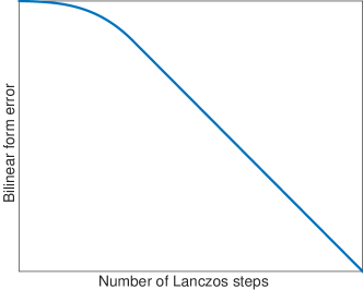
(a) Slow decrease initially

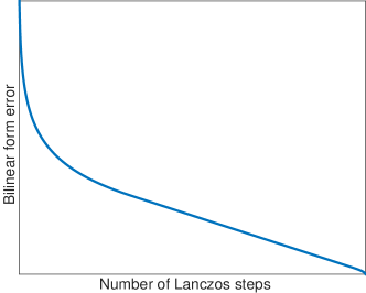
(b) Fast decrease initially

Figure 1: Pictorial illustration of the logarithmic bilinear form error over Lanczos iterations.

An example of the scenario illustrated in Figure 1(a) is that the incremental errors $d_{m}^{K}$ admit a decreasing ratio $d_{2}^{K}/d_{1}^{K}\geq d_{3}^{K}/d_{2}^{K}\geq\cdots$. One may show simply through induction that in such a case, the bilinear form errors $\rho_{m}^{K}$ also admit a decreasing ratio $\rho_{2}^{K}/\rho_{1}^{K}\geq\rho_{3}^{K}/\rho_{2}^{K}\geq\cdots$, which gives a concave shape of the error curve. Then, we obtain the same bound as that in Proposition 5, which is a special case of the following result.

Proposition 6.

Let $\{a_{i}\}_{i=1}^{n-1}$ be a positive and nonincreasing sequence and let $\{a_{i+1}/a_{i}\}_{i=1}^{n-2}$ be nonincreasing as well. Given $m$, $m^{\prime}>m$, and $t<1$ such that $a_{m^{\prime}}/a_{m}\leq t$, we have

$$\frac{\sum_{i=m^{\prime}}^{n-1}a_{i}}{\sum_{i=m}^{m^{\prime}-1}a_{i}}\leq\begin{cases}t/(1-t),&\text{if }n-m^{\prime}>m^{\prime}-m,\\ t,&\text{otherwise}.\end{cases}$$

Proof.

Let $a_{m^{\prime}}/a_{m^{\prime}-1}=c$. Then, because $a_{i+1}/a_{i}$ is nonincreasing for all $i$, we have

$$a_{m^{\prime}}+a_{m^{\prime}+1}+\cdots+a_{n-1}\leq a_{m^{\prime}}(1+c+c^{2}+\cdots+c^{n-m^{\prime}-1})$$

and

$$a_{m}+a_{m+1}+a_{m^{\prime}-1}\geq a_{m}(1+c+c^{2}+\cdots+c^{m^{\prime}-m-1}).$$

Therefore,

$$\frac{\sum_{i=m^{\prime}}^{n-1}a_{i}}{\sum_{i=m}^{m^{\prime}-1}a_{i}}\leq\frac{a_{m^{\prime}}(1-c^{n-m^{\prime}})}{a_{m}(1-c^{m^{\prime}-m})}\leq t\,\,\frac{1-c^{n-m^{\prime}}}{1-c^{m^{\prime}-m}}.$$

Furthermore, from

$$t\geq\frac{a_{m^{\prime}}}{a_{m}}=\frac{a_{m+1}}{a_{m}}\frac{a_{m+2}}{a_{m+1}}\cdots\frac{a_{m^{\prime}}}{a_{m^{\prime}-1}}\geq\left(\frac{a_{m^{\prime}}}{a_{m^{\prime}-1}}\right)^{m^{\prime}-m}=c^{m^{\prime}-m},$$

we conclude the proof by noting that if $n-m^{\prime}>m^{\prime}-m$, then $(1-c^{n-m^{\prime}})/(1-c^{m^{\prime}-m})\leq 1/(1-c^{m^{\prime}-m})\leq 1/(1-t)$; otherwise, $(1-c^{n-m^{\prime}})/(1-c^{m^{\prime}-m})\leq 1$. ∎

On the other hand, an example of the scenario illustrated in Figure 1(b) is that the incremental errors $d_{m}^{K}$ admit an increasing ratio $d_{2}^{K}/d_{1}^{K}\leq d_{3}^{K}/d_{2}^{K}\leq\cdots$. The worst case is that there exist two consecutive integers $m$ and $m^{\prime}=m+1$ such that the ratio $d_{m+1}^{K}/d_{m}^{K}$ is quite small (e.g., lower than the threshold $t$), but the incremental errors afterward decay too slowly, such that the cumulative error $d_{m,m^{\prime}}^{K}$ constitutes only a tiny portion of the overall error $\rho_{m}^{K}$. Hence, we consider a case where the incremental errors cannot abruptly change. In particular, let us assume that the beginning of the sequence $\{d_{m}^{K}\}$ is proportional to $m^{-(p+1)}$ for some $p>0$. At a certain point (when $m=s$), the sequence decreases at a constant rate, which results in an exponential decay pattern of the bilinear form error. The rate $c$ is equal to $(s-1)^{p+1}/s^{p+1}$ such that the transition of the decaying patterns is smooth. For this scenario, we have the following result.

Proposition 7.

Let $\{a_{i}\}_{i=m}^{n-1}$ be a sequence

$$\frac{1}{m^{p+1}},\,\,\frac{1}{(m+1)^{p+1}},\,\,\ldots,\frac{1}{(s-1)^{p+1}},\,\,\frac{1}{s^{p+1}},\,\,\frac{c}{s^{p+1}},\,\,\ldots,\frac{c^{n-s-1}}{s^{p+1}}$$

for some integer $s\in(m,n)$ and real number $p>0$, where $c=(s-1)^{p+1}/s^{p+1}$. Given integer $m^{\prime}\in(m,s)$ and $t<1$ such that $a_{m^{\prime}}/a_{m}\leq t$, we have

$$\frac{\sum_{i=m^{\prime}}^{n-1}a_{i}}{\sum_{i=m}^{m^{\prime}-1}a_{i}}\leq\dfrac{1+\frac{p}{m^{\prime}}-\left(\frac{m^{\prime}}{s}\right)^{p}\left[1+\frac{p}{s}-\frac{p}{p+1}\frac{1}{1-p/(2s)}\right]}{t^{-\frac{p}{p+1}}-1}.$$

Proof.

Because $1/x^{p+1}$ is monotonically decreasing for $x>0$, from the definition of integral (area under curve), we have for any positive integers $i$ and $j$ where $j>i$,

$$\frac{1}{i^{p+1}}+\cdots+\frac{1}{(j-1)^{p+1}}\geq\int_{i}^{j}\frac{dx}{x^{p+1}}=\frac{1}{p}\left(\frac{1}{i^{p}}-\frac{1}{j^{p}}\right),$$

and

$$\frac{1}{i^{p+1}}+\cdots+\frac{1}{(j-1)^{p+1}}\leq\int_{i}^{j}\frac{dx}{x^{p+1}}+\left(\frac{1}{i^{p+1}}-\frac{1}{j^{p+1}}\right)=\frac{1}{p}\left(\frac{1}{i^{p}}-\frac{1}{j^{p}}\right)+\left(\frac{1}{i^{p+1}}-\frac{1}{j^{p+1}}\right).$$

Therefore,

$$a_{m^{\prime}}+\cdots+a_{n-1} =\frac{1}{(m^{\prime})^{p+1}}+\cdots+\frac{1}{(s-1)^{p+1}}+\frac{1}{s^{p+1}}+\cdots+\frac{c^{n-s-1}}{s^{p+1}}$$

$$\leq\frac{1}{p}\left(\frac{1}{(m^{\prime})^{p}}-\frac{1}{s^{p}}\right)+\left(\frac{1}{(m^{\prime})^{p+1}}-\frac{1}{s^{p+1}}\right)+\frac{1}{s^{p+1}}\frac{1-c^{n-s}}{1-c},$$

and

$$a_{m}+\cdots+a_{m^{\prime}-1}\geq\frac{1}{p}\left(\frac{1}{m^{p}}-\frac{1}{(m^{\prime})^{p}}\right).$$

Hence, the ratio

$$\frac{\sum_{i=m^{\prime}}^{n-1}a_{i}}{\sum_{i=m}^{m^{\prime}-1}a_{i}}\leq\dfrac{1-\left(\frac{m^{\prime}}{s}\right)^{p}+\frac{p}{m^{\prime}}-\left(\frac{m^{\prime}}{s}\right)^{p}\frac{p}{s}+\left(\frac{m^{\prime}}{s}\right)^{p}\frac{p}{s}\frac{1-c^{n-s}}{1-c}}{\left(\frac{m^{\prime}}{m}\right)^{p}-1}.$$ (14)

Moreover, from $a_{m^{\prime}}/a_{m}\leq t$ we have

$$\left(\frac{m^{\prime}}{m}\right)^{p}=\left[\left(\frac{a_{m}}{a_{m^{\prime}}}\right)^{-\frac{1}{p+1}}\right]^{p}\geq t^{-\frac{p}{p+1}},$$ (15)

and from $c=(s-1)^{p+1}/s^{p+1}$ we have

$$1-c=1-\left(1-\frac{1}{s}\right)^{p+1}\geq 1-\left[1-\frac{p+1}{s}+\frac{(p+1)p}{2s^{2}}\right]=\frac{p+1}{s}\left(1-\frac{p}{2s}\right).$$ (16)

Then, substituting (15) and (16), together with the fact that $1-c^{n-s}<1$, into (14), we reach the inequality result of the proposition. ∎

The bound in Proposition 7 is slightly more obscure than that of Proposition 6, but it offers a qualitative interpretation. When $p\ll m^{\prime}$ and $s$, the terms $p/m^{\prime}$ and $p/s$ in the numerator are nearly zero, and hence the bound reads

$$\frac{\sum_{i=m^{\prime}}^{n-1}a_{i}}{\sum_{i=m}^{m^{\prime}-1}a_{i}}\lessapprox\dfrac{1-\frac{1}{p+1}\left(\frac{m^{\prime}}{s}\right)^{p}}{t^{-\frac{p}{p+1}}-1}.$$ (17)

When $p\geq 1$, we could even enlarge the right-hand side by omitting the term $\frac{1}{p+1}\left(\frac{m^{\prime}}{s}\right)^{p}$, which results in a bound $\left(t^{-\frac{p}{p+1}}-1\right)^{-1}$. If $t=0.1$, this bound $\leq 0.47$, sufficient for error estimation. When $p<1$, the term $\frac{1}{p+1}\left(\frac{m^{\prime}}{s}\right)^{p}$ may be nonnegligible, especially when $m^{\prime}$ is not too far from $s$. This term offsets the possibly small value of $t^{-\frac{p}{p+1}}-1$. The net result is that the bound (17) is not too large. For example, if $m^{\prime}/s=0.5$, then the bound $\leq 0.74$, again sufficient for error estimation.

4 Overall algorithm and parameter setting

With the developments in the preceding sections, we now summarize the overall algorithm that includes both approximating $\operatorname{tr}(f(A))$ and estimating the approximation error. Details are shown in Algorithm 2.

4.1 Algorithm

The procedure begins with approximating $\operatorname{tr}(f(A))$ by using $N$ independent and unbiased samples $u_{i}^{T}f(A)u_{i}$. Each sample is in turn approximated by $\|u_{i}\|^{2}e_{1}^{T}f(T_{m})e_{1}$ based on the Lanczos method. Here, $m$ is the number of Lanczos steps and it is implicitly determined by an error tolerance $\delta$ that ensures that the difference between $u_{i}^{T}f(A)u_{i}$ and $\|u_{i}\|^{2}e_{1}^{T}f(T_{m})e_{1}$ is bounded by the tolerance. To estimate the difference between these two quantities (termed “bilinear form error”) at each Lanczos step $m$, an incremental error $d_{m}^{K}$ is computed based on a simple recurrence summarized in Algorithm 1. Then, an estimate of the bilinear form error, termed “cumulative error,” is computed based on the incremental errors.

To be specific, we need to trace back a few steps (say, at step $\underline{m}<m$) to obtain an accurate approximation of the bilinear form error. Therefore, the algorithmic progression is opposite to how the cumulative error is defined in the preceding section (where we used the notation $m<m^{\prime}$ and thought forwardly). Algorithmically, we say that $d_{\underline{m},m}^{K}$ is an accumulation of the incremental errors from $d_{\underline{m}}^{K}$ to $d_{m-1}^{K}$. Hence, whenever a new incremental error is obtained in a certain Lanczos step, it is added to the cumulative errors for all the previous steps (see line 9 of Algorithm 2). We maintain a threshold $t=0.1$. For every $m$, there is an associated $\underline{m}$ that is the smallest integer satisfying $|d_{m}^{K}|/|d_{\underline{m}}^{K}|\geq t$. If at some step $m$ with the associated $\underline{m}$, the cumulative error $d_{\underline{m},m}^{K}$ falls below the scaled tolerance $\delta/\|u_{i}\|^{2}$, then we consider that the bilinear form approximation $\|u_{i}\|^{2}e_{1}^{T}f(T_{\underline{m}})e_{1}$ has converged to $u_{i}^{T}f(A)u_{i}$ within a tolerance $\delta$. This concludes the computation of $u_{i}^{T}f(A)u_{i}$.

Algorithm 2 Estimating $\operatorname{tr}(f(A))$ with confidence interval

1:Matrix $A$, function $f$, number $N$ of random vectors, Lanczos tolerance $\delta$, threshold $t=0.1$

2:If needed by line 3, estimate the spectrum interval of $A$

3:Obtain a rational approximation of $f$ (in the spectrum interval)

4:loop $i=1,2,\ldots,N$

5:     Generate a random vector $u_{i}$ and use $u_{i}/\|u_{i}\|$ as the starting vector of Lanczos

6:     loop $m=1,2,\ldots$

7:         Run one step of Lanczos; perform reorthogonalization if necessary

8:         Compute incremental error $d_{m}^{K}$ (i.e., lines 3–8 of Algorithm 1)

9:         Update cumulative error $d_{\underline{m},m}^{K}\leftarrow d_{\underline{m},m}^{K}+d_{m}^{K}$ for all $\underline{m}<m$

10:         Find the smallest integer $\underline{m}<m$ such that $t|d_{\underline{m}}^{K}|\leq|d_{m}^{K}|$

11:         If $|d_{\underline{m},m}^{K}|<\delta/\|u_{i}\|^{2}$, signal convergence and exit the current loop

12:     end loop

13:     Obtain an approximation $\|u_{i}\|^{2}e_{1}^{T}f(T_{\underline{m}})e_{1}$ of the unbiased sample $u_{i}^{T}f(A)u_{i}$

14:end loop

15:Obtain an estimate of $\operatorname{tr}(f(A))$ with $N$ samples

16:Obtain a confidence interval for the estimate by using Theorem 1

4.2 Parameters

Two parameters related to the error estimation deserve some attention.

In principle, the Lanczos tolerance $\delta$ is free, because Theorem 1 is applicable to any positive $\delta$. In practice, it is not sensible to make $\delta$ too small or too large. In the former case the uncertainty in the statistical error dominates, whereas in the latter case the numerical bias dominates. A reasonable approach is to make these two sources of errors comparable; i.e., let $\delta=\beta\alpha s^{(m)}/\sqrt{N}$ for some $\beta\approx 1$ (see Corollary 2). The conundrum of this approach is that the sample standard error $s^{(m)}$ is unknown. To resolve the issue, one could run Algorithm 2 once as a precomputation, but omit all the unnecessary overheads. That is, no error estimation is performed, and the sample size $N^{\prime}$ needs only be sufficient for the sample standard error to stabilize (e.g., $N^{\prime}=30$), but it needs not be as large as $N$.

The number of poles, $K$, must be sufficiently large such that the error in the rational approximation of $f$ does not compromise the estimation of the bilinear form error. Based on Theorem 4, we will require that the uniform error of $f-r_{K}$ be at most $\frac{1}{2}\delta/\|u_{i}\|^{2}$. When the random vectors $u_{i}$ are symmetric Bernoulli vectors, each $u_{i}$ has a constant 2-norm $\sqrt{n}$.

5 Experiments with 2D Laplacian

To test the effectiveness of the proposed method, we first verify the several algorithmic components with the 2D Laplacian matrix on an $n_{1}\times n_{2}$ grid:

$$A=I_{n_{2}\times n_{2}}\otimes L_{n_{1}\times n_{1}}+L_{n_{2}\times n_{2}}\otimes I_{n_{1}\times n_{1}},$$

where $I$ is the identity matrix, $L$ is the 1D Laplacian matrix $\text{tridiag}(-1,2,-1)$, and the subscripts denote the matrix size. This matrix is sparse and is well suited for the Lanczos method that heavily relies on matrix-vector multiplications. Moreover, its eigenvalues and eigenvectors are known. In particular, $A$ is increasingly ill conditioned (with a condition number $\approx 4n/\pi^{2}$ for a square grid $n_{1}=n_{2}$) and the matrix of normalized eigenvectors coincides with the matrix of discrete sine transform. Hence, the ground truth $\operatorname{tr}(f(A))$ can be computed economically, with an $O(n\log n)$ cost, through fast sine transform.

The experiments in this section consist of three parts: (a) the effectiveness of rational approximations for several commonly used functions $f$; (b) the effectiveness of error estimation for the bilinear form $v_{1}^{T}f(A)v_{1}$; and (c) the effectiveness of the overall error estimation for $\operatorname{tr}(f(A))$ in the form of a confidence interval. Although rational approximations are not the contribution of this work, the purpose of part (a) is to obtain an empirical understanding of the needed number of poles, $K$.

5.1 Rational approximation

We consider four functions with known fast-converging rational approximations: the negative exponential $\exp(-x)$, the square root $\sqrt{x}$, the logarithm $\log(x)$, and a composite of hyperbolic tangent and square root $\tanh(\sqrt{x})$, all used for $x>0$. These approximations are related to quadratures of contour integrals, as we briefly motivated in Section 3.2. The details for the exponential appear in Trefethen et al. [38], who discussed approximations derived from both Talbot quadratures and best uniform approximations. The details for the latter three functions appear in Hale et al. [21], who proposed using the trapezoid rule on conformal mappings of the circular contour. The resulting approximations in Hale et al. [21] are dependent on the spectrum interval of $A$.

Minor modifications are needed for our use. For the exponential, discussions in Trefethen et al. [38] are based on $\exp(x)$, $x\leq 0$; hence, we need to flip the sign of $x$ and accordingly negate the coefficients and poles, such that they agree with the canonical form (6). Moreover, because both the coefficients and the poles come in conjugate pairs, we may keep only one from each pair, multiply the coefficients by $2$, and extract the real part of the sum. This results in the form (7), reducing the number of summation terms in (6) by half. We will use the best uniform approximation rather than Talbot quadratures because it converges twice as fast. For Matlab codes, see Figure 4.1 of Trefethen et al. [38].

For the logarithm $\log(x)$ and the composite $\tanh(\sqrt{x})$, we will use Method 2 and Method 1 of Hale et al. [21], respectively. The formulas therein are in the form of neither (6) nor (7): an additional multiplicative term $A$ appears in the front and the imaginary part of a summation is extracted instead of the real part. Hence, we turn to the quadrature formula before the imaginary part is extracted, rewrite the formula into the canonical form (6) plus a constant, and extract the real part of the summation as done for the exponential discussed above (which results in the same effect of reducing summation terms by half). The additional constant term attached to the canonical form (6) cancels out when the quadrature is used for approximating the bilinear form error (cf. (8)); hence, it barely matters.

For the square root $\sqrt{x}$, we will use Method 3 of Hale et al. [21]. No modifications are needed. Note that the poles are all on the negative real axis.

We plot in Figure 2 the error $|f-r_{K}|$, where recall that $r_{K}$ is the rational approximation with $K$ terms. For the exponential, the interval is $[0,8]$ and for the other functions, the interval is $[10^{-6},1]$. As can be seen, for the exponential, a very small number of points suffices to decrease the uniform error to approximately machine precision. For the other functions, $K$ needs to be larger, but often one or a few dozen points are sufficient.

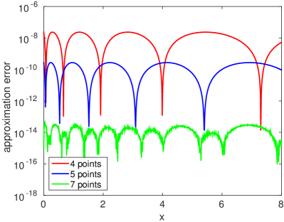
(a) $f(x)=\exp(-x)$

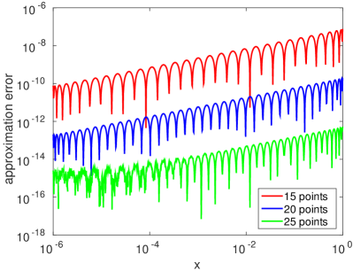
(b) $f(x)=\sqrt{x}$

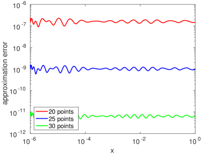
(c) $f(x)=\log(x)$

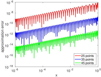
(d) $f(x)=\tanh(\sqrt{x})$

Figure 2: Rational approximation of various functions $f$ by using $K$ quadrature points.

5.2 Error estimation for the bilinear form

We use a $300\times 400$ grid as an example. The ground truth $v_{1}^{T}f(A)v_{1}$ for any vector $v_{1}$ may be computed by using fast sine transform, as explained earlier. Here, we choose $v_{1}$ to be the random vector of iid (independent and identically distributed) symmetric Bernoulli variables, normalized to the unit norm. The Lanczos approximation $e_{1}^{T}f(T_{m})e_{1}$ with $m$ Lanczos steps is then computed and the error is plotted as the blue solid curve in Figure 3.

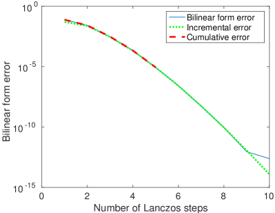
(a) $f(x)=\exp(-x)$

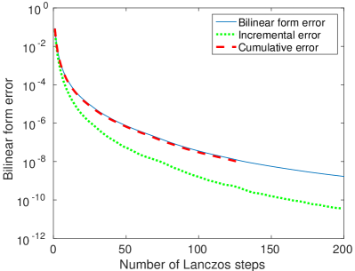
(b) $f(x)=\sqrt{x}$

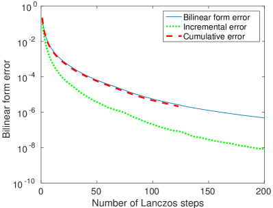
(c) $f(x)=\log(x)$

(d) $f(x)=\tanh(\sqrt{x})$

Figure 3: Bilinear form error and estimates, for 2D Laplacian matrix on a $300\times 400$ grid.

To estimate this error, we compute the incremental error $d_{m}^{K}$ and the cumulative error $d_{m,m^{\prime}}^{K}$, where $m^{\prime}$ is the smallest integer greater than $m$ such that $|d_{m^{\prime}}^{K}|/|d_{m}^{K}|\leq t$. The absolute value of these errors is plotted as the green and red dashed curves in the figure, respectively. Clearly, we may plot only the $d_{m,m^{\prime}}^{K}$’s that satisfy $m^{\prime}\leq 200$, which is the maximum number of Lanczos steps seen in Figure 3.

As can be seen, for the exponential, the three errors nearly overlap. It is for this reason that we do not plot the whole red curve; otherwise, it fully covers the green curve. The extremely fast convergence implies that the incremental error suffices as an estimate of the bilinear form error. For the other functions, the incremental error is far from the bilinear form error, and hence it is necessary to do an accumulation to get a better estimate. The fact that the curve of cumulative errors nearly overlaps with that of the bilinear form errors indicates that the accumulation criterion is effective.

5.3 Overall error estimation with confidence interval

With the preparation of the preceding two subsections, we now apply Theorem 1 to establish confidence intervals for the approximation of $\operatorname{tr}(f(A))$. To this end, we fix the number $N$ of random vectors to be $100$ and set $\alpha=3$, which ensures a high probability $p_{\alpha}\approx 99.73\%$. We vary the size of the matrix $A$ (and hence the condition number) by using progressively larger grids. The setting of the number of quadrature points, $K$, and the Lanczos tolerance $\delta$ follows Section 4.2.

We perform the computations and summarize the results in Tables 1 and 2. As the grid becomes larger, the condition number of $A$ increases, which leads to a larger $\delta$ and $K$. Interestingly, for the largest grid (which corresponds to $n\approx 10^{6}$), $K=3$ quadrature points are sufficient for the exponential, and for other functions, $K$ does not exceed two dozens. Then, the resulting accuracy of the rational approximation is five to six digits. The number of Lanczos steps, $m$, is as small as $6$ for the exponential and no greater than $34$ for the logarithm, on average. Moreover, the approximated trace is generally three- to four-digit accurate, and the half-width of the confidence interval is generally a few times the actual error (in several cases, mostly for large problems, it is less than twice the actual error). As expected, the time for estimating the error is negligible compared with that for approximating the trace.

Note that for this problem, the implementation of the Lanczos algorithm does not affect timing much, even using full reorthogonalization. It turns out that the accuracies are barely affected by the loss of orthogonality, possibly because 2D Laplacians are easy to handle. For later experiments, however, reorthogonalization is crucial because the approximation error substantially degrades without it (see an illustration in the appendix). In these experiments, the matrix may be much larger and Lanczos converges more slowly. Hence, to gain time efficiency, it will be beneficial to replace the simple full reorthogonalization therein by a more sophisticated scheme such as partial reorthogonalization [33, 12]. Therefore, we implemented and used partial reorthogonalization for all experiments in this paper. For more details on the implementation and the machine setting, see the next section.

Table 1: Approximately computing $\operatorname{tr}(f(A))$ with $99.73\%$ confidence interval for 2D Laplacian matrix $A$. In all cases, the number $N$ of random vectors is $100$.

$f(x)=\exp(-x)$
Grid size	90$\times$120	300$\times$400	900$\times$1200
# Quadrature points, $K$	2	3	3
Rational approx. error	1.72e-04	2.01e-06	2.01e-06
Lanczos tolerance $\delta$	8.31	26.1	71
Average # of Lan. steps, $m$	5	5	6
Truth $\mu=\operatorname{tr}(f(A))$	1014.96	11378.0	102662
Approximation result $\bar{x}^{(m)}$	1016.38	11367.3	102630
99.73% Confidence interval	$\pm$19.14	$\pm$60.1	$\pm$164
Time approximation (seconds)	0.28	2.12	21.75
Time error estimate (seconds)	0.01	0.02	0.04

$f(x)=\sqrt{x}$
Grid size	90$\times$120	300$\times$400	900$\times$1200
# Quadrature points, $K$	6	8	10
Rational approx. error	2.71e-04	9.65e-05	3.99e-05
Lanczos tolerance $\delta$	25.1	80	220
Average # of Lan. steps, $m$	5.04	7.07	10.01
Truth $\mu=\operatorname{tr}(f(A))$	20708.0	229986	2.06961e+06
Approximation result $\bar{x}^{(m)}$	20715.9	230071	2.06984e+06
99.73% Confidence interval	$\pm$57.7	$\pm$185	$\pm$507
Time approximation (seconds)	0.43	4.56	53.39
Time error estimate (seconds)	0.01	0.04	0.10

Table 2: (Continued from Table 1) Approximately computing $\operatorname{tr}(f(A))$ with $99.73\%$ confidence interval for 2D Laplacian matrix $A$. In all cases, the number $N$ of random vectors is $100$.

$f(x)=\log(x)$
Grid size	90$\times$120	300$\times$400	900$\times$1200
# Quadrature points, $K$	9	10	14
Rational approx. error	2.82e-04	6.56e-04	4.64e-05
Lanczos tolerance $\delta$	38.0	120	314
Average # of Lan. steps, $m$	10.16	18.19	33.29
Truth $\mu=\operatorname{tr}(f(A))$	12652.9	140146	1.26014e+06
Approximation result $\bar{x}^{(m)}$	12672.4	140319	1.26060e+06
99.73% Confidence interval	$\pm$87.5	$\pm$277	$\pm$723
Time approximation (seconds)	0.90	13.11	194.38
Time error estimate (seconds)	0.04	0.16	0.49

$f(x)=\tanh(\sqrt{x})$
Grid size	90$\times$120	300$\times$400	900$\times$1200
# Quadrature points, $K$	12	15	20
Rational approx. error	6.84e-05	3.68e-05	9.77e-06
Lanczos tolerance $\delta$	5.73	18	48
Average # of Lan. steps, $m$	8.00	11.25	16.17
Truth $\mu=\operatorname{tr}(f(A))$	9928.62	110240	991960
Approximation result $\bar{x}^{(m)}$	9930.14	110261	992025
99.73% Confidence interval	$\pm$13.13	$\pm$41	$\pm$110
Time approximation (seconds)	0.66	6.49	83.08
Time error estimate (seconds)	0.03	0.08	0.19

6 Experiments with covariance matrices

In this section, we present experiments with covariance matrices encountered in Gaussian process analysis [35, 29, 1, 36]. A Gaussian process is a stochastic process with Gaussian properties. Central to the mathematical tool is a covariance kernel function that generates a covariance matrix $A$ for sampling sites, where the observations collectively follow a multivariate normal distribution with covariance $A$. Many tasks, including hyperparameter estimation and prediction, require a computation with the matrix $A$. Here, we focus on the log-determinant term that appears in the Gaussian log-likelihood, which needs to be optimized for estimating the hyperparameters of the process. Clearly, for a symmetric positive-definite matrix $A$,

$$\log\det(A)=\operatorname{tr}(\log(A)).$$

For demonstration, we will use the Matérn kernel function plus a nugget

$$\phi(r)=\frac{(\sqrt{2\nu}r)^{\nu}\mathsf{K}_{\nu}(\sqrt{2\nu}r)}{2^{\nu-1}\Gamma(\nu)}+\tau\cdot\delta(r=0)\quad\text{with}\quad r=\sqrt{\sum_{i=1}^{d}\frac{(x_{i}-x^{\prime}_{i})^{2}}{\ell_{i}^{2}}}$$

as an example. Here $x=[x_{1},x_{2},\ldots,x_{d}]$ denotes a site in ^d, $r$ denotes the elliptical distance between two sites $x$ and $x^{\prime}$ with elliptical scaling $[\ell_{1},\ell_{2},\ldots,\ell_{d}]$, $\mathsf{K}_{\nu}$ is the modified Bessel function of the second kind of order $\nu$, $\Gamma(\nu)$ is the Gamma function, $\delta(r=0)$ is the Kronecker delta taking $1$ when $r=0$ and $0$ otherwise, and $\tau$ is the size of the nugget. The Matérn kernel (even without the nugget) is strictly positive-definite, meaning that the generated matrix $A=[\phi(x-x^{\prime})]$ for all pairs of sites $x$ and $x^{\prime}$ is positive-definite. The Matérn kernel is even, achieves its maximum $1$ at the origin, and monotonically decreases when $r>0$.

We assume that the sites are located on a regular grid of size $n_{1}\times n_{2}$ and set the scaling parameters to be $\ell_{1}=0.4\times n_{2}$ and $\ell_{2}=0.4\times n_{1}$. We also set the smoothness parameter $\nu=1.5$ and the nugget $\tau=10^{-5}$. With a regular grid structure, matrix-vector multiplications with $A$ has an $O(n)$ memory and $O(n\log n)$ time cost, although $A$ is fully dense, because the multiplications may be done through circulant embedding followed by fast Fourier transform (FFT) [7, 10].

To make the experiment more interesting, we let the sites be $10\%$ uniformly random samples of the grid (i.e., the number of sites $n=0.1\times n_{1}n_{2}$). Hence, strictly speaking, the sites no longer form a regular grid; they are scattered sites. However, matrix-vector multiplications may still be performed through circulant embedding and FFT, because of the underlying grid structure. Note, nevertheless, that the cost is not reduced by a factor of $10$ as is the case for the number of sites.

Unlike the 2D Laplacian in the preceding section, the spectral information of the covariance matrix is only partially known. In particular, we know that the smallest eigenvalue of $A$ has a lower bound $\tau$ (the nugget) but do not know the largest eigenvalue. In theory, the largest eigenvalue grows approximately proportionally with $n$ and the smallest eigenvalue decreases to $\tau$ fairly quickly [8]. Hence, we estimate the largest eigenvalue by using the Lanczos method and set the lower end of the spectrum interval to be $\tau$. By using this spectrum interval we obtain a rational approximation of $f(x)=\log(x)$, needed for error estimation.

As mentioned at the end of the preceding subsection, we implemented the Lanczos iteration (1) with partial reorthogonalization [33, 12]. The reason is that, as will be seen soon, the number of Lanczos steps is no longer as small as those in the case of 2D Laplacian and so the reorthogonalization cost is quite high if full reorthogonalization is used.

The program is written in Matlab and run on a laptop with eight Intel cores (CPU frequency 2.8GHz) and 32GB memory. By default, Matlab uses four threads in many built-in functions, but we observe that at most two cores are active during the computation.

In Table 3, we summarize the computation results for varying grid sizes from $160\times 90$ to $1600\times 900$. For the first two grids, performing spectral decomposition is affordable and hence we also compute the ground-truth condition numbers and log-determinants. As can be seen, using the nugget $\tau$ (lower bound) as an estimate of the smallest eigenvalue suffices for indicating the magnitude of the condition number. As expected, the condition number grows approximately by a factor of $10$ every time we increase the grid size by this factor. With an increasing condition number, the log-determinant is harder to compute, requiring more Lanczos steps. Note that the scale of this number—in the hundreds—is much larger than that for the 2D Laplacian. Taking another factor into account, namely the matrix size, it takes quite some time to finish the computation (for the largest grid, several hours), although the costs of the spectrum estimation and error estimation are negligible. The benefit, on the other hand, is that we have a useful error bound for the approximated trace, which gives a confidence in the computation which would have been impossible without a reliable error estimate.

Table 3: Approximately computing $\log\det(A)$ with $99.73\%$ confidence interval for covariance matrix $A$. In all cases, the number $N$ of random vectors is $100$.

Grid size	160$\times$90	500$\times$300	1600$\times$900
Condition number (truth)	4.08e+07	5.54e+08	---
Condition number (estimated)	5.17e+07	5.60e+08	5.22787e+09
# Quadrature points, $K$	12	15	18
Rational approx. error	5.19e-03	1.39e-03	4.18e-04
Lanczos tolerance $\delta$	40.5	99	288
Average # of Lan. steps, $m$	103	240	425
Truth $\mu=\log\det(A)$	-10844.7	-151826	---
Approximation result $\bar{x}^{(m)}$	-10794.3	-151715	-1.60122e+06
99.73% Confidence interval	$\pm$92.6	$\pm$228	$\pm$480
Time spectrum estim. (seconds)	0.04	0.3	3
Time trace approx. (seconds)	26.87	781.6	14253
Time error estimate (seconds)	0.43	1.9	3

7 Concluding remarks

In this work, we proposed two error estimates related to the computation of $f(A)$: one for its bilinear form and one for its trace. The bilinear form is a building block of the trace in a Monte Carlo-type approximation. We focused on the symmetric positive-definite case for $A$, where the Lanczos algorithm has long been a preferred iterative method and where a representative application is the covariance matrix, whose log-determinant (i.e., $f(x)=\log(x)$) constitutes a significant computational component of Gaussian process analysis.

The bilinear form $v_{1}^{T}f(A)v_{1}$ is approximated by $e_{1}^{T}f(T_{m})e_{1}$, where $v_{1}$, if normalized, is the starting vector of Lanczos, and $T_{m}$ is the tridiagonal matrix resulting from $m$ steps of the Lanczos process. The approximation error is gauged through economically accumulating incremental errors $d_{k}=e_{1}^{T}f(T_{k+1})e_{1}-e_{1}^{T}f(T_{k})e_{1}$ for $k=m,m+1,m+2\ldots$, because eventually $v_{1}^{T}f(A)v_{1}$ is nothing but $e_{1}^{T}f(T_{n})e_{1}$ if $A$ has a size $n\times n$. The challenging question is how many terms one should accumulate in order to obtain a reasonable, yet economic, estimate of the approximation error, because these terms require running extra Lanczos iterations beyond the $m$-th one. Our proposal is that one should accumulate till $k=m^{\prime}-1$, where $|d_{m^{\prime}}/d_{m}|$ falls under some threshold $t$, a reasonable choice being $0.1$. Such a proposal is motivated by two facts: (i) if the even derivatives of $f$ have the same sign, then so are the incremental errors $d_{k}$; and (ii) if $f$ is analytic in the spectrum interval of $A$ and analytically continuable inside an open Bernstein ellipse whose foci are the two ends of the interval, then Lanczos converges exponentially. Many functions in practical applications for positive-definite matrices incidentally meet these two criteria, including those used in our experiments: $\exp(-x)$, $\log(x)$, and $x^{\alpha}$ for $\alpha<1$. This leaves room for future investigations as to whether the proposal is more generally applicable to functions without the constant-sign property for its even derivatives.

In retrospect, our proposal resembles that of Frommer et al. [15] in several ways. Even though their work focused on rational functions, our work in effect also relies on rational approximations of a general function. Their Lanczos restart recovery strategy corresponds to our idea of running extra Lanczos iterations. A crucial distinction, however, is that the number of extra Lanczos iterations in our case is determined implicitly by the requirement $|d_{m^{\prime}}/d_{m}|\leq 0.1$, whereas this number needs be prescribed in advance in Frommer et al. [15] The benefit of an implicit determination over a prescribed one is a much more accurate estimate, independent of the convergence speed. On the other hand, prescribing a good number of extra Lanczos steps for sharp estimates likely requires an a priori knowledge of the convergence behavior.

The second contribution of our work is the error estimation of the trace. The trace $\operatorname{tr}(f(A))$ is approximated by a Monte Carlo sample average of $u_{i}^{T}f(A)u_{i}$, where the $u_{i}$’s are independent random vectors and each sample $u_{i}^{T}f(A)u_{i}$ is unbiased. Therefore, the approximation error generally follows basic estimation theory, where confidence intervals are established as a means for bounding the error in a (high) probability. The distinction, however, is that the samples (the bilinear forms) are only approximately computed and hence they bear a numerical bias. Our strategy is to impose a bound $\delta$ (as a stopping criterion for the bilinear form approximation) on the numerical bias and inject $\delta$ into the confidence interval. Such a treatment is quite general, overcoming the limitation of a prior work [9] applicable to only multivariate normal vectors $u_{i}$. A restriction, on the other hand, is that the setting of a reasonable $\delta$ is relatively blind before computation, whereas the prior work proposes directly the tolerance that matches the numerical error with the statistical error. If one wants a $\delta$ that makes these two sources of errors comparable in the framework of this work, a practical approach is to run a precomputation (the same as Algorithm 2 but without error estimate), get an approximate standard error of the samples, and follow Corollary 2.

Appendix A Effects of loss of orthogonality

We illustrate in Figure 4 that the Lanczos convergence for $v_{1}^{T}\log(A)v_{1}$ substantially degrades without reorthogonalization.

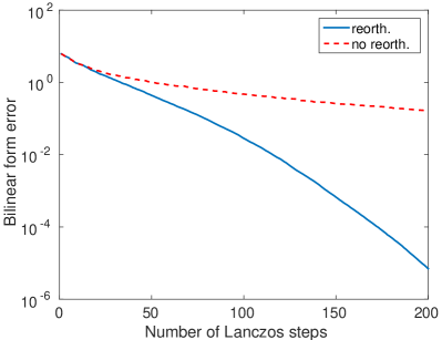
Figure 4: Convergence history of $v_{1}^{T}\log(A)v_{1}$ for $A$ defined in Section 6 on a $90\times 120$ grid.

References

- [1] M. Anitescu, J. Chen, and L. Wang. A matrix-free approach for solving the parametric Gaussian process maximum likelihood problem. SIAM J. Sci. Comput., 34(1):A240–A262, 2012.
- [2] H. Avron and S. Toledo. Randomized algorithms for estimating the trace of an implicit symmetric positive semi-definite matrix. J. Assoc. Comput. Mach., 58(2), 2011.
- [3] Z. Bai, G. Fahey, and G. Golub. Some large-scale matrix computation problems. J. Comput. Appl. Math., 74(1-2):71–89, 1996.
- [4] C. Bekas, E. Kokiopoulou, and Y. Saad. An estimator for the diagonal of a matrix. Appl. Numer. Math., 57(11-12):1214–1229, 2007.
- [5] M. Bellalij, L. Reichel, G. Rodriguez, and H. Sadok. Bounding matrix functionals via partial global block Lanczos decomposition. Appl. Numer. Math., 94:127–139, 2015.
- [6] C. Brezinski, P. Fika, and M. Mitrouli. Estimations of the trace of powers of positive self-adjoint operators by extrapolation of the moments. Electronic Transactions on Numerical Analysis, 39:144–155, 2012.
- [7] R. H. Chan and X.-Q. Jin. An Introduction to Iterative Toeplitz Solvers. SIAM, 2007.
- [8] J. Chen. On the use of discrete Laplace operator for preconditioning kernel matrices. SIAM J. Sci. Comput., 35(2):A577–A602, 2013.
- [9] J. Chen. How accurately should I compute implicit matrix-vector products when applying the Hutchinson trace estimator? SIAM J. Sci. Comput., 38(6):A3515–A3539, 2016.
- [10] J. Chen, T. L. H. Li, and M. Anitescu. A parallel linear solver for multilevel Toeplitz systems with possibly several right-hand sides. Parallel Comput., 40(8):408–424, 2014.
- [11] E. Estrada. Characterization of 3D molecular structure. Chemical Physics Letters, 319(5–6):713–718, 2000.
- [12] H.-R. Fang and Y. Saad. A filtered Lanczos procedure for extreme and interior eigenvalue problems. SIAM J. Sci. Comput., 34(4):A2220–A2246, 2012.
- [13] P. Fika and M. Mitrouli. Estimation of the bilinear form for Hermitian matrices. Linear Algebra and its Applications, 502:140–158, 2016.
- [14] P. Fika, M. Mitrouli, and P. Roupa. Estimating the diagonal of matrix functions. Mathematical Methods in the Applied Sciences, 2016.
- [15] A. Frommer, K. Kahl, Th. Lippert, and H. Rittich. 2-norm error bounds and estimates for Lanczos approximations to linear systems and rational matrix functions. SIAM J. Matrix Anal. Appl., 34(3):1046–1065, 2013.
- [16] A. Frommer and V. Simoncini. Error bounds for Lanczos approximations of rational functions of matrices. In Numerical Validation in Current Hardware Architectures, volume 5492 of Lecture Notes in Computer Science, pages 203–216. Springer Berlin Heidelberg, 2009.
- [17] D Girard. Un algorithme simple et rapide pour la validation croisée généralisée sur des problèmes de grande taille. Technical Report RR 669-M, Inf. et Math. Appl. de Grenoble, Grenoble, France, 1987.
- [18] G. H. Golub and G. Meurant. Matrices, Moments and Quadrature with Applications. Princeton University Press, 2009.
- [19] G. H. Golub and U. von Matt. Generalized cross-validation for large-scale problems. J. Comp. Graph. Stat., 6(1):1–34, 1997.
- [20] G.H. Golub and J.H. Welsch. Calculation of Gauss quadrature rules. Math. Comp., 23:221–230, 1969.
- [21] N. Hale, N. J. Higham, and L. N. Trefethen. Computing , and related matrix functions by contour integrals. SIAM J. Numer. Anal., 46(5):2505–2523, 2008.
- [22] I. Han, D. Malioutov, H. Avron, and J. Shin. Approximating the spectral sums of large-scale matrices using Chebyshev approximations. arXiv:1606.00942, 2016.
- [23] I. Han, D. Malioutov, and J. Shin. Large-scale log-determinant computation through stochastic Chebyshev expansions. In Proceedings of the 32nd International Conference on Machine Learning, 2015.
- [24] M. F. Hutchinson. A stochastic estimator of the trace of the influence matrix for Laplacian smoothing splines. Communications in Statistics – Simulation and Computation, 19:433–450, 1990.
- [25] G. López Lagomasino, L. Reichel, and L. Wunderlich. Matrices, moments, and rational quadrature. Linear Algebra Appl., 429(10):2540–2554, 2008.
- [26] L. Lin. Randomized estimation of spectral densities of large matrices made accurate. Numerische Mathematik, 136(1):183–213, 2017.
- [27] L. Lin, Y. Saad, and C. Yang. Approximating spectral densities of large matrices. SIAM Rev., in press.
- [28] C. Meurant. Estimates of the trace of the inverse of a symmetric matrix using the modified Chebyshev algorithm. Numerical Algorithms, 51(3):309–318, 2009.
- [29] C. E. Rasmussen and C. K. I. Williams. Gaussian Processes for Machine Learning. The MIT Press, 2006.
- [30] F. Roosta-Khorasani and U. Ascher. Improved bounds on sample size for implicit matrix trace estimators. Foundations of Computational Mathematics, 15(5):1187–1212, 2015.
- [31] Y. Saad. Analysis of some Krylov subspace approximations to the matrix exponential operator. SIAM J. Numer. Anal., 29(1):209–228, 1992.
- [32] Y. Saad. Iterative Methods for Sparse Linear Systems. SIAM, 2nd edition, 2003.
- [33] H. D. Simon. The Lanczos algorithm with partial reorthogonalization. Math. Comp., 42(165):115–142, 1984.
- [34] A. Stathopoulos, J. Laeuchli, and K. Orginos. Hierarchical probing for estimating the trace of the matrix inverse on toroidal lattices. SIAM J. Sci. Comput., 35(5):S299–S322, 2013.
- [35] M. L. Stein. Interpolation of Spatial Data: Some Theory for Kriging. Springer, 1999.
- [36] M. L. Stein, J. Chen, and M. Anitescu. Stochastic approximation of score functions for Gaussian processes. Annals of Applied Statistics, 7(2):1162–1191, 2013.
- [37] L. N. Trefethen. Approximation Theory and Approximation Practice. Society for Industrial and Applied Mathematics, 2012.
- [38] L. N. Trefethen, J.A.C. Weideman, and T. Schmelzer. Talbot quadratures and rational approximations. BIT Numerical Mathematics, 46(653–670), 2006.
- [39] K. Wimmer, Y. Wu, and P. Zhang. Optimal query complexity for estimating the trace of a matrix. In Proceedings of the 41st International Colloquium on Automata, Languages and Programming, 2014.
- [40] L. Wu, A. Stathopoulos, J. Laeuchli, V. Kalantzis, and E. Gallopoulos. Estimating the trace of the matrix inverse by interpolating from the diagonal of an approximate inverse. Journal of Computational Physics, 326(1):828–844, 2016.