Bias Correction Estimation for Continuous-Time Asset Return Model with Jumps

Abstract

In this paper, local linear estimators are adapted for the unknown infinitesimal coefficients associated with continuous-time asset return model with jumps, which can correct the bias automatically due to their simple bias representation. The integrated diffusion models with jumps, especially infinite activity jumps are mainly investigated. In addition, under mild conditions, the weak consistency and asymptotic normality is provided through the conditional Lindeberg theorem. Furthermore, our method presents advantages in bias correction through simulation whether jumps belong to the finite activity case or infinite activity case. Finally, the estimators are illustrated empirically through the returns for stock index under five-minute high sampling frequency for real application.

1 Introduction

Continuous-time models are widely used in economics and finance, such as interest rate etc, especially the continuous-time diffusion processes with jumps. Jump-diffusion process $X_{t}$ is represented by the following stochastic differential equation:

$$dX_{t}=\mu(X_{t-})dt+\sigma(X_{t-})dW_{t}+\int_{\mathscr{E}}c(X_{t-},z)r(\omega,dt,dz),$$ (1.1)

which can accommodate the impact of sudden and large shocks to financial markets. Johannes [23] provided the statistical and economic role of jumps in continuous-time interest rate models. However, in empirical finance the current observation usually behaves as the cumulation of all past perturbation such as stock prices by means of asset returns in Nicolau [30] et al. Furthermore, in the research field involved with model (1.1), although the scholars focused on the price of the asset, most of them didn't consider the returns of the asset. As mentioned in Campbell, Lo and MacKinlay [3], return series of an asset are a complete and scale-free summary of the investment opportunity for most investors, and are easier to handle than price series due to their more attractive statistical properties. The capital asset return model is the core of capital market theory which describes the relationship between the returns and risks of individual securities or portfolio.

For characterizing this integrated economic phenomenon, moreover, the return series, we considered the promising continuous-time integrated diffusion process with jumps (1.2), which is motivated by unit root processes under the discrete framework of Park and Phillips [31] and continuous integrated diffusion process in Nicolau [29]. It satisfies the following second-order stochastic differential equation:

$$\left\{\begin{array}[]{ll}dY_{t}=X_{t}dt,\\ dX_{t}=\mu(X_{t-})dt+\sigma(X_{t-})dW_{t}+\int_{\mathscr{E}}c(X_{t-},z)r(\omega,dt,dz),\end{array}\right.$$ (1.2)

where $\mathscr{E}=\mathbb{R}\setminus\{0\},$ $W=\{W_{t}\}_{t\geq 0}$ is a standard Brownian motion, $r(\omega,dt,dz)=(p-q)(dt,dz),~{}p(dt,dz)$ is a time-homogeneous Poisson random measure on $\mathbb{R}_{+}\times\mathbb{R}$, which is independent of $W_{t}$, and $q(dt,dz)$ is its intensity measure, that is, $E[p(dt,dz)]=q(dt,dz)=f(z)dzdt$, $f(z)$ is a Lévy density. For empirical financial data, $X_{t}$ in the model (1.2) represents the continuously compounded return of underlying assets, $Y_{t}$ denotes the asset price by means of the cumulation of the returns plus initial asset value. Furthermore, the model (1.2) can accommodate nonstationarity and transform nonstationarity into stationarity by differencing, which can not be performed through univariate diffusion model due to the nondifferentiability of a Brownian motion.

For model (1.2), the estimators for unknown coefficients have been considered based on low frequency or high frequency observations under various settings. For model (1.2) without jumps, Gloter [15][16] and Ditlevsen and Sørensen [8] built the parametric and semiparametric estimation, while Nicolau [29] and Comte, Genon-Catalot and Rozenholc [4] analyzed nonparametric estimators for the unknown quantities. Moreover, Wang and Lin [38], Wang, Zhang and Tang [40], Hanif [19] and Wang and Tang [39] improved the nonparametric estimators for them. For model (1.2) with finite activity jumps, Song and Lin [35], Song, Lin and Wang [36], Chen and Zhang [7] and Funke and Schmisser [13] theoretically investigated nonparametric estimation for the drift or volatility coefficients. Song [34] empirically considered the application for the estimation proposed in high frequency financial data.

In this paper, we adapt local linear estimators for the unknown coefficients of integrated diffusion models with jumps, especially infinite activity jumps. In the context of nonparametric estimator with finite-dimensional auxiliary variables, local polynomial smoothing become an effective smoothing method, which doesn't assume the functional form for the unknown coefficients. Moreover, local linear estimators have excellent properties such as full asymptotic minimax efficiency achievement and boundary bias correction automatically, one can refer to Fan and Gijbels [10] for better review.

Our contribution have three folds. Firstly, in terms of the model, the previous work was mainly focused on the continuous case as Nicolau [29] or finite activity case as Song [34]. We will consider a more practical integrated diffusion models with infinite activity jumps for the asset return. The existence of infinite activity jumps for the high frequency financial data has been testified based on Aït-Sahalia and Jacod [1] in empirical analysis part.

Secondly, in the theoretical side, compared with Nadaraya-Watson estimators, the conditional Lindeberg theorem might be no longer applicable for the local linear estimators due to their destroyed adaptive and predictable structure of conditionally on the $\sigma-$field generated by $X_{t}.$ We effectively tackle the key technical problems by means of the Slutsky's theorem and establish central limit theorems for the volatility functions in the second-order diffusion model with infinite activity jumps. More technical proof details can be sketched in Lemma 4 and Theorem 2.6.

Thirdly, Chen and Zhang [7] gave the large sample properties of local linear estimators for second-order diffusion with finite activity jump, but they didn't consider the finite-sampling performance of them. Considering what has been talked above, in the practical side we consider two types of jump (finite activity jumps and infinite activity jumps) aimed at verifying the better finite-sampling performance of local linear estimators under various settings. Moreover, the estimators are illustrated empirically through the return of stock index in Shenzhen Stock Exchange under five-minute high sampling frequency data between Jan 2015 and Dec 2015. In summary, the integrated diffusion model with jump, especially infinite activity jumps may be an alternative model to describe the dynamic variation for the returns of financial assets.

The paper is organized as follows. The local linear estimators and their large sample properties are collected in Section 2. The finite sample performance of underlying estimators through Monte Carlo simulation study is presented in Section 3. The estimators are illustrated empirically in Section 4. Some technical lemmas for the main theorems are given in Appendix part.

2 Local Linear estimators and Large sample properties

For model (1.2), we usually get observations $\{Y_{i\Delta_{n}};i=1,2,\cdot\cdot\cdot\}$ rather than $\{X_{i\Delta_{n}};i=1,2,\cdot\cdot\cdot\}.$ However, the value of $X_{t_{i}}$ cannot be obtained from $Y_{t_{i}}=Y_{0}+\int_{0}^{t_{i}}X_{s}ds$ in a fixed sample intervals. Additionally, nonparametric estimations of the unknown qualities in model (1.2) cannot in principle be constructed on the observations $\{Y_{i\Delta_{n}};i=1,2,\cdot\cdot\cdot\}$ due to the unknown conditional distribution of $Y$. As Nicolau [29] showed, with observations $\{Y_{i\Delta_{n}};i=1,2,\cdot\cdot\cdot\}$ and given that

$$Y_{{i\Delta_{n}}}-Y_{{(i-1)\Delta_{n}}}=\int_{(i-1)\Delta_{n}}^{i\Delta_{n}}X_{u}du,$$

we can obtain an approximation value of $X_{i\Delta_{n}}$ by

$$\widetilde{X}_{i\Delta_{n}}=\frac{Y_{i\Delta_{n}}-Y_{(i-1)\Delta_{n}}}{\Delta_{n}}.$$ (2.1)

Due to the Markov properties of model (1.2), we can build the following infinitesimal conditional expectations

$$E\left[\frac{\widetilde{X}_{(i+1)\Delta_{n}}-\widetilde{X}_{i\Delta_{n}}}{\Delta_{n}}|\mathscr{F}_{(i-1)\Delta_{n}}\right]=\mu(X_{(i-1)\Delta_{n}})+O_{p}(\Delta_{n}),$$ (2.2)

$$E\left[\frac{(\widetilde{X}_{(i+1)\Delta_{n}}-\widetilde{X}_{i\Delta_{n}})^{2}}{\Delta_{n}}|\mathscr{F}_{(i-1)\Delta_{n}}\right]=\frac{2}{3}\sigma^{2}(X_{(i-1)\Delta_{n}})+\frac{2}{3}\int_{\mathbb{R}}c^{2}(X_{(i-1)\Delta_{n}},z)f(z)dz+O_{p}(\Delta_{n}).$$ (2.3)

where $\mathscr{F}_{t}=\sigma\{X_{s},s\leq t\}$. One can refer to Appendix A in Song, Lin and Wang [36] for detailed calculations.

For the given $\{\widetilde{X}_{i\Delta_{n}};i=1,2,\cdots\}$, the local linear estimators for $\mu(x)$ and $M(x)$ based on infinitesimal conditional expectations (2.2) and (2.3) are defined as the solutions to the following weighted least squares problems: find $a_{1}$, $b_{1}$, $a_{2}$, $b_{2}$ to minimize

$$\sum_{i=1}^{n}\Big{(}\frac{\widetilde{X}_{(i+1)\Delta_{n}}-\widetilde{X}_{i\Delta_{n}}}{\Delta_{n}}-a_{1}-b_{1}\big{(}{\widetilde{X}_{i\Delta_{n}}-x}\big{)}\Big{)}^{2}K\Big{(}\frac{\widetilde{X}_{(i-1)\Delta_{n}}-x}{h_{n}}\Big{)},$$ (2.4)

$$\sum_{i=1}^{n}\Big{(}\frac{\frac{3}{2}(\widetilde{X}_{(i+1)\Delta_{n}}-\widetilde{X}_{i\Delta_{n}})^{2}}{\Delta_{n}}-a_{2}-b_{2}\big{(}{\widetilde{X}_{i\Delta_{n}}-x}\big{)}\Big{)}^{2}K\Big{(}\frac{\widetilde{X}_{(i-1)\Delta_{n}}-x}{h_{n}}\Big{)},$$ (2.5)

where $K(\cdot)$ is the kernel function and $h_{n}$ is a sequence of positive numbers, satisfies $h_{n}\to 0$ as $n\to\infty.$

The solutions for $a_{1}$ and $a_{2}$ to (2.4) and (2.5) as follows are respectively the local linear estimators of $\mu(x)$ and $M(x)=\sigma^{2}(x)+\int_{\mathscr{E}}c(x,z)f(z)dz,$

$$\hat{\mu}_{n}(x)=\frac{\sum_{i=1}^{n}\omega_{i-1}\Big{(}\frac{\widetilde{X}_{i+1}-\widetilde{X}_{i}}{\Delta_{n}}\Big{)}}{\sum_{i=1}^{n}\omega_{i-1}},$$ (2.6)

$$\hat{M}_{n}(x)=\frac{\sum_{i=1}^{n}\omega_{i-1}\frac{3}{2}\frac{(\widetilde{X}_{i+1}-\widetilde{X}_{i})^{2}}{\Delta_{n}}}{\sum_{i=1}^{n}\omega_{i-1}}$$ (2.7)

where

$$\omega_{i-1}=K\left(\frac{\widetilde{X}_{i-1}-x}{h_{n}}\right)\Bigg{(}\sum_{j=1}^{n}K\left(\frac{\widetilde{X}_{j-1}-x}{h_{n}}\right)(\widetilde{X}_{j}-x)^{2}-(\widetilde{X}_{i}-x)\sum_{j=1}^{n}K\left(\frac{\widetilde{X}_{j-1}-x}{h_{n}}\right)(\widetilde{X}_{j}-x)\Bigg{)}.$$

The assumptions of this paper are listed below, which confirm the large sample properties of the constructed estimators based on (2.6) and (2.7).

Assumption 1

i) (Local Lipschitz continuity)  For each $n\in\mathbb{N},$ there exist a constant $L_{n}$ and a function $\zeta_{n}$ : $\mathscr{E}\rightarrow\mathbb{R}_{+}$ with $\int_{\mathscr{E}}\zeta_{n}^{2}(z)\nu(dz)<\infty$ such that, for any $|x|\leq n,|y|\leq n,z\in{\mathscr{E}}$,

$$|\mu(x)-\mu(y)|+|\sigma(x)-\sigma(y)|\leq L_{n}|x-y|,~{}~{}~{}|c(x,z)-c(y,z)|\leq\zeta_{n}(z)|x-y|.$$

(ii (Linear growthness)  For each $n\in\mathbb{N}$, there exist $\zeta_{n}$ as above and C, such that for all $x\in\mathbb{R},z\in{\mathscr{E}}$,

$$|\mu(x)|+|\sigma(x)|\leq C(1+|x|),~{}|c(x,z)|\leq\zeta_{n}(z)(1+|x|).$$

Remark 2.1

This assumption guarantees the existence and uniqueness of a solution to stochastic differential equation $X_{t}$ in (1.2), see Jacod and Shiryaev [22]. For instance, Long, Ma and Shimizu [26] and Long and Qian [27] imposed similar conditions on the coefficients of the underlying stochastic differential equation.

Assumption 2

The process $X=\{X_{t}\}_{\geq 0}$ is ergodic and stationary with a finite invariant measure $\phi(x)$. For a given point $x_{0}$, the stationary probability measure $p(x)$ of the process $X$ is positive at $x_{0},$ that is $p(x_{0})>0.$ Furthermore, the process $X$ is $\rho-$mixing with $\sum_{i\geq 1}\rho(i\Delta_{n})=O(\frac{1}{\Delta_{n}^{\alpha}}),~{}n\rightarrow\infty,$ where $\alpha<1/2.$

Remark 2.2

The Assumption 2 implies that the process $X_{t}$ has a unique weak solution. The finite invariant measure implies that the process $X_{t}$ is positive Harris recurrent with the stationary probability measure $p(x)=\frac{\phi(x)}{\phi(\mathscr{D})},~{}\forall x\in\mathscr{D}.$ The hypothesis that $X_{t}$ is a stationary process is obviously a plausible assumption because for major integrated time series data, a simple differentiation generally assures stationarity. The same condition yielding information on the rate of decay of $\rho-$mixing coefficients for $X_{t}$ was mentioned the Assumption 3 in Gugushvili and Spereij [17]. For instance, the $\rho-$mixing process $X_{t}$ with exponentially decreasing mixing coefficients satisfies the condition, see Hansen and Scheinkman [20], Chen, Hansen and Carrasco [5].

Assumption 3

The kernel $K$($\cdot$) : $\mathbb{R}\rightarrow\mathbb{R}^{+}$ is a positive and continuously differentiable function satisfying:

$$\int K(u)du=1,~{}K_{i}^{j}:=\int K^{i}(u)u^{j}du<\infty.$$

Moreover, For $2\leq i\leq n$,

$$\lim_{h\rightarrow 0}E\left[~{}\frac{1}{h}~{}|K^{{}^{\prime}}(\xi_{n,i})|^{\alpha}\Big{(}\frac{\widetilde{X}_{(i-1)\Delta_{n}}-x}{h}\Big{)}^{m}\right]<\infty$$

where $\alpha=1,2$ or $4$, $m=0,1$ or $2$ and $\xi_{n,i}$ = $\theta\left(\frac{X_{(i-1)\Delta_{n}}-x}{h}\right)+(1-\theta)\left(\frac{\widetilde{X}_{(i-1)\Delta_{n}}-x}{h}\right)$, $0\leq\theta\leq 1.$

Remark 2.3

In fact, any density function can be considered as a kernel, moreover even unnecessary positive functions can be used. For simplification, we only consider positive and symmetrical kernels used widely. It is well known both empirically and theoretically that the choice of kernel functions is not very important to the kernel estimator, see Gasser and Müller [14]. As Nicolau [29] pointed out this assumption is generally satisfied under very weak conditions. For instance, with a Gaussian kernel and a Cauchy stationary density (which has heavy tails) we still have $\lim_{h\rightarrow 0}E\big{[}(\frac{1}{h})|K^{{}^{\prime}}(\frac{X}{h})|^{4}\big{]}<\infty$. Notice that the expectation with respect to the distribution $\xi_{n,i}$ depends on the stationary densities of $X_{n,i}$ and $\widetilde{X}_{n,i}$ because $\xi_{n,i}$ is a convex linear combination of $X_{n,i}$ and $\widetilde{X}_{n,i}.$

Assumption 4

For every $p\geq 1$, $\sup_{t\geq 0}E[|X_{t}|^{p}]<\infty,$ and $\int_{\mathscr{E}}|z|^{p}\nu(dz)<\infty.$

Remark 2.4

This assumption guarantees that Lemma 1 can be used properly throughout the article. If $X$ is a Lévy process with bounded jumps (i.e., $\sup_{t}|\Delta X_{t}|\leq C<\infty$ almost surely, where C is a nonrandom constant), then $E\{|X_{t}^{n}|\}<\infty~{}\forall n$, that is, $X_{t}$ has bounded moments of all orders, see Protter [32]. This condition is widely used in the estimation of an ergodic diffusion or jump-diffusion from discrete observations, see Florens-Zmirou [11], Kessler [24], Shimizu and Yoshida [33].

Assumption 5

$\Delta_{n}\rightarrow 0,~{}(\frac{n\Delta_{n}}{h_{n}})(\Delta_{n}\log(\frac{1}{\Delta_{n}}))^{\frac{1}{2}}\rightarrow 0,~{}h_{n}n\Delta_{n}^{1+\alpha}\rightarrow\infty,h_{n}^{5}n\Delta_{n}\rightarrow 0~{}as~{}n\rightarrow\infty.$

Remark 2.5

The relationship between $h_{n}$ and $\Delta_{n}$ is similar as the stationary case in Bandi and Nguyen [2] and (b1), (b2) of A8 in Nicolau [29].

We have the following asymptotic results for the local linear estimators such as (2.6) and (2.7) based on the assumptions above.

Theorem 2.6

Under Assumptions 1-5, as $n\rightarrow\infty,$ we have

(i)  $\hat{\mu}_{n}(x)\stackrel{{\scriptstyle P}}{{\longrightarrow}}\mu(x),~{}\hat{M}_{n}(x)\stackrel{{\scriptstyle P}}{{\longrightarrow}}M(x).$

(ii) Furthermore, if $h_{n}n\Delta_{n}\longrightarrow 0$ and $h_{n}=O((n\Delta_{n})^{-1/5}),$ then

$$\sqrt{h_{n}n\Delta_{n}}\left(\hat{\mu}_{n}(x)-\mu(x)-\frac{1}{2}h_{n}^{2}\mu^{{}^{\prime\prime}}(x)\frac{(K_{1}^{2})^{2}-K_{1}^{3}K_{1}^{1}}{K_{1}^{2}-(K_{1}^{1})^{2}}\right)\Longrightarrow N\left(0,V\frac{M(x)}{p(x)}\right),$$

and

$$\sqrt{h_{n}n\Delta_{n}}\left(\hat{M}_{n}(x)-M(x)-\frac{1}{2}h_{n}^{2}M^{{}^{\prime\prime}}(x)\frac{(K_{1}^{2})^{2}-K_{1}^{3}K_{1}^{1}}{K_{1}^{2}-(K_{1}^{1})^{2}}\right)\Longrightarrow N\left(0,V\frac{\int_{\mathscr{E}}c^{4}(x,y)f(y)dy}{p(x)}\right),$$

where

$$V=\frac{(K_{1}^{2})^{2}K_{2}^{0}+(K_{1}^{1})^{2}K_{2}^{2}-2(K_{1}^{1})(K_{1}^{2})K_{2}^{1}}{[K_{1}^{2}-(K_{1}^{1})^{2}]^{2}}.$$

Remark 2.7

For the finite activity jumps of model (1.2),

$$\int_{\mathscr{E}}c(X_{t-},z)r(\omega,dt,dz):=\int_{\mathscr{E}}c(X_{t-},z)N(dt,dz)-\lambda(X_{t-})\int_{\mathscr{E}}c(X_{t-},z)\Pi(dz)dt,$$

where $N(dt,dz)$ is a Poisson counting measure, $c(\cdot,y)$ reflects the conditional impact of a jump and $\Pi(dz)$ is the probability distribution function of a jump. For model (1.2), we can observe that $f(z)=\lambda(x)\Pi(z),$ so $M(x)=\sigma^{2}(x)+\lambda(x)\int_{\mathscr{E}}c^{2}(x,z)\Pi(dz)$ and $\int_{\mathscr{E}}c^{4}(x,z)f(z)dz=\lambda(x)\int_{\mathscr{E}}c^{4}(x,z)\Pi(dz).$

For the infinite activity jumps of model (1.2), we will focus on the following diffusion process with jumps for $X_{t}$ such that

$$dX_{t}=\mu(X_{t-})dt+\sigma(X_{t-})dW_{t}+\xi(X_{t-})dJ_{t},$$

where $J_{t}$ is a pure jump Lévy process such as an infinite activity jump process of the representation

$$dJ_{t}=\int_{\mathbb{R}}y(\mu(dt,dy)-\nu(dy)dt):=\int_{\mathbb{R}}y\bar{\mu}(dt,dy)$$

with $\mu(dt,dy)$ a Poisson random measure compensated by its intensity measure $\nu(dy)dt.$ Hence $M(x)=\sigma^{2}(x)+\int_{\mathscr{R}}c^{2}(x,z)\nu(dz)$ and $\int_{\mathscr{R}}c^{4}(x,z)f(z)dz=\int_{\mathscr{R}}c^{4}(x,z)\nu(dz)$ for model (1.2).

In contrary to the integrated diffusion model without jumps (Nicolau [29]), the rate of convergence of the second infinitesimal moment estimator is same as the first infinitesimal moment estimator. Apparently, this is due to the presence of discontinuous breaks that have an equal impact on all the functional estimates. As Johannes [23] pointed out, for the conditional variance of interest rate changes, not only diffusion play a certain role, but also jumps account for more than half at lower interest level rates, almost two-thirds at higher interest level rates, which dominate the conditional volatility of interest rate changes. Thus, it is extremely important to estimate the conditional variance as $\sigma^{2}(x)$ + $\int_{\mathscr{E}}c^{2}(x,z)f(z)dz$ which reflects the fluctuation of the return of the underlying asset.

Remark 2.8

In Song [34], he showed that under the Assumptions in this paper, $h_{n}n\Delta_{n}\rightarrow 0$ and $h_{n}=O((n\Delta_{n})^{-1/5}),$ the following result holds with symmetric kernels

$$\sqrt{h_{n}n\Delta_{n}}\left(\hat{\mu}^{NW}_{n}(x)-\mu(x)-h_{n}^{2}K_{1}^{2}\left(\frac{1}{2}\mu^{{}^{\prime\prime}}(x)+\mu^{{}^{\prime}}(x)\frac{\phi^{{}^{\prime}}(x)}{\phi(x)}\right)\right)\stackrel{{\scriptstyle d}}{{\rightarrow}}N\Big{(}0,K_{2}^{0}\frac{M(x)}{p(x)}\Big{)}.$$

When $K$ is symmetric, for local linear estimators we obtain that

$$\sqrt{h_{n}n\Delta_{n}}\left(\hat{\mu}_{n}(x)-\mu(x)-\frac{1}{2}h_{n}^{2}\mu^{{}^{\prime\prime}}(x)K_{1}^{2}\right)\Longrightarrow N\left(0,K_{2}^{0}\frac{M(x)}{p(x)}\right).$$

Comparing the bias of local linear estimator with that of Nadaraya-Watson estimator in Song [34] above, we can observe that the bias of $\hat{\mu}_{n}^{NW}-\mu(x)$ is $\mu^{{}^{\prime}}(x)\frac{\phi^{{}^{\prime}}(x)}{\phi(x)}K_{1}^{2}$ more than that of $\hat{\mu}_{n}(x)-\mu(x)$. When $K$ is asymmetric, sketching the proof procedure in Song [34], we can prove that the bias for $\hat{\mu}^{NW}-\mu(x)$ should subtract $hK_{1}^{1},$ which confirms the bias of local linear estimator is smaller than that of Nadaraya-Watson case. Hence, compared with the Nadaraya-Watson estimator, local linear estimator possesses simple bias representation and can correct the bias automatically whether $K(\cdot)$ is symmetric or not.

Remark 2.9

Similarly as Theorem 4 in Fan and Gijbels [9], we now investigate the behavior of the estimator (2.6) at left-boundary points (the right-boundary points are the same). Put $x_{n}=ch_{n}$, with $c>0$. Assuming $nh_{n}\rightarrow\infty$, the conditional MSE of the estimator (2.6) at the boundary point $x_{n}$ is $O(h_{n}^{4}+\frac{1}{nh_{n}})$. More proof details see Fan and Gijbels [9] (A little tedious, so we omit here). Indeed, its rate of convergence for local linear estimator is not influenced by the position of the point under consideration. Hence the local linear smoother does not require modifications at the boundary. So it turns out that the local linear smoother has an additional advantage over other kernel-type estimator (see Gasser and Müller [14]). To some extend, the simulation in the paper confirms this result.

Remark 2.10

It is very important to consider the choice of the bandwidth in nonparametric estimation. Here we will select the optimal bandwidth $h_{n}$ based on the mean squared error (MSE) and the asymptotic theory in Theorem 2.6. Take $\mu(x)$ for example, the optimal smoothing parameter $h_{n}$ for local linear estimator of $\mu(x)$ is given that

$$h_{n,opt,fi}=\left(\frac{1}{n\Delta_{n}}\cdot\frac{4VM(x)(K_{1}^{2}-(K_{1}^{1})^{2})^{2}}{p(x)\mu^{2^{\prime\prime}}(x)((K_{1}^{2})^{2}-K_{1}^{3}K_{1}^{1})^{2}}\right)^{\frac{1}{5}}=O_{p}\left(\frac{1}{n\Delta_{n}}\right)^{\frac{1}{5}},$$

which differs from the continuous case with $h_{n,opt}=O_{p}({n}^{-1/5}).$ The bandwidth $h_{n}$ constructed above relies on the consistent estimators for these unknown quantities and they are difficult to obtain and may give rise to bias. Here we mention two rules of thumb on selecting the bandwidth. Practically, for simplicity one can use the empirical bandwidth selector $h_{n}=1.06*\hat{S}*(n\Delta_{n})^{-1/5},$ where $\hat{S}$ denotes the standard deviation of the data. Or, one can apply the cross-validation method to assess the performance of an estimator via estimating its prediction error. The main idea is to minimize the following expression: $CV(h)=n^{-1}\sum_{i=1}^{n}\{\frac{\widetilde{X}_{(i+1)\Delta_{n}}-\widetilde{X}_{i\Delta_{n}}}{\Delta_{n}}-\hat{a}_{h,-i}(\widetilde{X}_{i\Delta_{n}})\}^{2}$, where $\hat{a}_{h,-i}(\widetilde{X}_{i\Delta_{n}})$ is the local linear estimator (2.6) and bandwidth $h$, but without using the $i$th observation.

Remark 2.11

If the smoothing parameter $h_{n}=O((n\Delta_{n})^{-1/5}),$ the normal confidence interval for $\mu(x)$ using local linear estimators at the significance level $100(1-\alpha)\%$ are constructed as follows,

$$I_{\mu,\alpha}= \Bigg{[}\hat{\mu}_{n}(x)-h_{n}^{2}\cdot\frac{1}{2}\hat{\mu}_{n}^{{}^{\prime\prime}}(x)\frac{(K_{1}^{2})^{2}-K_{1}^{3}K_{1}^{1}}{K_{1}^{2}-(K_{1}^{1})^{2}}-z_{1-\alpha/2}\cdot\frac{1}{\sqrt{n\Delta_{n}h_{n}}}\cdot\sqrt{V\frac{\hat{M}_{n}(x)}{\hat{p}_{n}(x)}},$$

$$\hat{\mu}_{n}(x)-h_{n}^{2}\cdot\frac{1}{2}\hat{\mu}_{n}^{{}^{\prime\prime}}(x)\frac{(K_{1}^{2})^{2}-K_{1}^{3}K_{1}^{1}}{K_{1}^{2}-(K_{1}^{1})^{2}}+z_{1-\alpha/2}\cdot\frac{1}{\sqrt{n\Delta_{n}h_{n}}}\cdot\sqrt{V\frac{\hat{M}_{n}(x)}{\hat{p}_{n}(x)}}\Bigg{]},$$

where $z_{1-\alpha/2}$ is the inverse CDF for the standard normal distribution evaluated at $1-\alpha/2.$ To facilitate statistical inference for $\mu(x)$ based on Theorem 2.6, we need to conduct consistent estimators for the unknown quantities in the normal approximation. $\hat{\mu}_{n}(x),$ $\hat{M}_{n}(x)$ denote the local linear estimators of $\mu(x),M(x)$ in (2.6) and (2.7), respectively. As Fan and Gijbels [10] showed, the derivative $\hat{\mu}_{n}^{{}^{\prime\prime}}(x)$ in $I_{\mu,\alpha}$ can be estimated by taking the second derivative of the local linear estimators of $\mu(x)$ in (2.6). The consistent estimator for $p(x)$ is

$$\hat{p}_{n}(x)=\frac{1}{nh_{n}}\sum_{i=1}^{n}K\left(\frac{\widetilde{X}_{(i-1)\Delta_{n}}-x}{h_{n}}\right).$$

3 Monte Carlo Simulation Study

In this section, a simple Monte Carlo simulation experiment is constructed aimed at the finite-sampling performance between local linear estimators constructed as (2.6) and (2.7) denoted as LL and Nadaraya-Watson estimators constructed in Song (2017) denoted as NW. Throughout this section, various lengths of observation time interval $T~{}(=50,100,500)$ and sample sizes $n~{}(=500,1000,2500)$ with $\Delta_{n}=\frac{T}{n}$ will be considered. We use classical Gaussian kernel $K(x)=\frac{1}{\sqrt{2\pi}}e^{-\frac{x^{2}}{2}}$ and the common bandwidth $h=1.06*\hat{S}*(n\Delta_{n})^{-\frac{1}{5}}=1.06*\hat{S}*T^{-\frac{1}{5}}$, where $\hat{S}$ denotes the standard deviation of the data. Here we will consider two types of jump aimed at verifying the better finite-sampling performance of local linear estimators under various settings. Take the estimator $\hat{\mu}_{n}(x)$ of $\mu(x)$ for example to show the small-sampling performance. Similar results can be found for $\hat{M}_{n}(x)$ of $M(x).$

Example 1 (Finite Activity case). Our experiment is based on the following second-order diffusion model with finite activity jump:

$$\left\{\begin{array}[]{ll}dY_{t}=X_{t-}dt,\\ dX_{t}=-10X_{t-}dt+\sqrt{0.1+0.1X_{t-}^{2}}dW_{t}+dJ_{t},\end{array}\right.$$ (3.1)

where the coefficients of continuous part are equal to the ones used in Nicolau [29] and $J_{t}$ is a compound Poisson jump process with arrival intensity $\lambda=2$ and jump size $Z_{n}\sim\mathscr{N}(0,0.036^{2})$ corresponding to Bandi and Nguyen [2].

The finite-sample performance of the local linear estimator and NW estimator for $\mu(x)$ with finite activity jump is demonstrated in Figure 1. We can observe that local linear estimator performs a little better than the NW estimator, especially at the boundary points. What is shown in Table 1 is the biases of local linear estimator and NW estimator at various quantile points of $X_{t}.$ In addition, 95% Monte Carlo confidence intervals of various estimators for $\mu(x)$ are depicted in Figure 2. It shows that the true value of $\mu(x)$ can not fall in the 95% Monte Carlo confidence intervals of NW estimators at the sparse design boundary points. These findings confirms the fact that local linear estimator can correct the boundary bias automatically due to its simple bias representation as shown in Remark 2.8. Figure 3 gives the QQ Plots for local linear estimator of the drift function $\mu(x)$ with finite activity jump, which reveals the normality of local linear estimators in finite sample and confirms the results in Theorems 2.6.

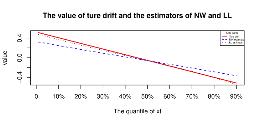
Figure 1: Various Nonparametric Estimators for $\mu(x)=-10*x$ with $T=10,~{}n=1000,~{}\lambda=2$ and jump size $Z_{n}\sim\mathscr{N}(0,0.036^{2})$

Table 1: The Biases of Nadaraya-Watson and Local Linear Estimators for $\mu(x)=-10*x$ at various quantile points of sample $X_{t}$ with $T=10,~{}n=1000,~{}\lambda=2$ and jump size $Z_{n}\sim\mathscr{N}(0,0.036^{2})$

Bias	Various Quantile Points of Sample Xt
	10%	20%	30%	40%	50%	60%	70%	80%	90%
NW	-0.1898	-0.1302	-0.0817	-0.0468	-0.0193	0.0178	0.0556	0.0965	0.1465
LL	-0.0668	-0.0388	-0.0232	-0.0161	-0.0131	-0.0128	-0.0178	-0.0305	-0.0600

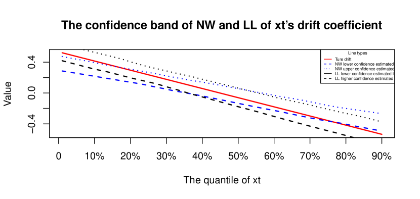
Figure 2: 95% Monte Carlo Confidence Interval for $\mu(x)=-10*x$ with $T=10,~{}n=1000,~{}\lambda=2$ and jump size $Z_{n}\sim\mathscr{N}(0,0.036^{2})$

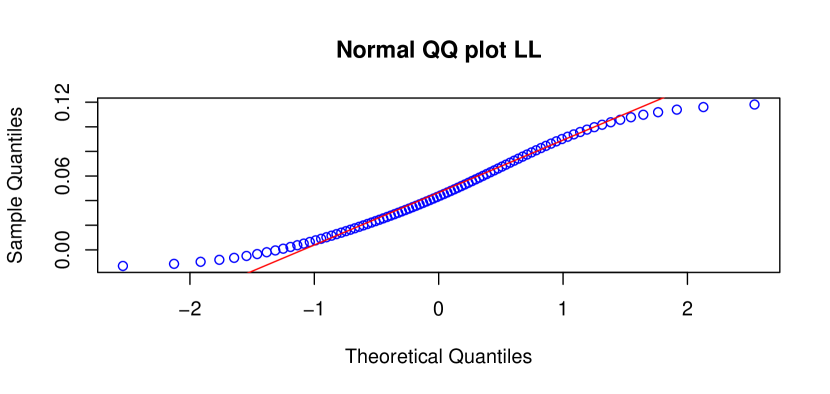
Figure 3: QQ plot of local linear estimator for $\mu(x)=-10*x$ with $T=10,~{}n=1000,~{}\lambda=2$ and jump size $Z_{n}\sim\mathscr{N}(0,0.036^{2})$

Next, we will assess the global performance between local linear estimator and NW estimator via the Root of Mean Square Errors (RMSE)

$$RMSE=\sqrt{\frac{1}{m}\sum_{k=0}^{m}\left\{\hat{\mu}(x_{k})-\mu(x_{k})\right\}^{2}},$$ (3.2)

where $\hat{\mu}(x)$ is the estimator of $\mu(x)$ and $\{x_{k}\}_{1}^{m}$ are chosen uniformly to cover the range of sample path of $X_{t}.$ Tables 2, 3 and 4 report the results on RMSE-LL and RMSE-NW for the drift function $\mu(x)$ with different types of time spans, sampling numbers, jump intensities and jump sizes over 100 replicates.

We can notice that the local linear estimator performs a little better (approximately reduced by half) than the NW estimator in terms of the RMSE under different types of time spans, sampling numbers, jump intensities and jump sizes. This fact confirms that local linear estimator possesses the property of bias correction. From Table 2, we can get the other two findings. Firstly, for the same time interval $T$, as the sample sizes $n$ tends larger, the performances of these estimators improved due to more information used for estimators. Secondly, for the same sample sizes $n$, as the time interval $T$ expands larger, the performances of these estimators get worse due to the fact that more jumps happened in larger time interval $T.$ From Table 3 and 4, for the same jump size or the same jump arrival intensity, as the sample sizes $n$ tends larger, the performances of the estimators for $\mu(x)$ are also improved due to the fact that more jump information for estimation procedure is collected as as $\Delta_{n}\rightarrow 0.$ However, for the same sample sizes $n$, as the amplitude or frequency of jump becomes larger, the RMSE of the estimators gradually becoming larger.

Table 2: Simulation results on RMSE-NW and RMSE-LL for three lengths of time interval (T) and three sample sizes for $\mu(x)=-10x$ with jump size $Z_{n}\sim\mathscr{N}(0,0.036^{2})$ and jump intensity $\lambda=2$ over 100 replicates.

Time Span	Estimators	$n=500$	$n=1000$	$n=2500$
$T=10$	RMSE-NW	0.2566	0.1403	0.1002
	RMSE-LL	0.1532	0.0813	0.0560
$T=20$	RMSE-NW	0.3734	0.2246	0.1334
	RMSE-LL	0.1033	0.0970	0.0947
$T=50$	RMSE-NW	0.9885	0.3907	0.1522
	RMSE-LL	0.2114	0.1492	0.0869

Table 3: Simulation results on RMSE-NW and RMSE-LL for three types of jump intensity $\lambda$ and three sample sizes for $\mu(x)=-10x$ with $T=10$ and jump size $Z_{n}\sim\mathscr{N}(0,0.036^{2})$ over 100 replicates.

Jump Intensity	Estimators	$n=500$	$n=1000$	$n=2500$
$\lambda=1$	RMSE-NW	0.2297	0.1117	0.0629
	RMSE-LL	0.0896	0.0892	0.0480
$\lambda=2$	RMSE-NW	0.2566	0.1403	0.1002
	RMSE-LL	0.1532	0.0813	0.0560
$\lambda=5$	RMSE-NW	0.3174	0.1763	0.1305
	RMSE-LL	0.1603	0.0950	0.0736

Table 4: Simulation results on RMSE-NW and RMSE-LL for three types of jump size $Z_{n}$ and three sample sizes for $\mu(x)=-10x$ with $T=10$ and jump intensity $\lambda=2$ over 100 replicates.

Jump Size	Estimators	$n=500$	$n=1000$	$n=2500$
$Z_{n}\sim\mathscr{N}(0,0.036^{2})$	RMSE-NW	0.2566	0.1403	0.1002
	RMSE-LL	0.1532	0.0813	0.0560
$Z_{n}\sim\mathscr{N}(0,1)$	RMSE-NW	0.4532	0.2031	0.1690
	RMSE-LL	0.2961	0.0931	0.0797
$Z_{n}\sim Cauchy(0,1)$	RMSE-NW	0.7983	0.2156	0.1830
	RMSE-LL	0.4083	0.1242	0.1538

Example 2 (Infinite Activity case). The infinite activity jump $J_{t}$ in second-order diffusion model (3.1) is a Variance Gamma (VG) jump process, that is $J_{t}=cG_{t}+\eta W_{G_{t}}$ with $c=-0.2,~{}\eta=0.2$, where $G_{t}$ is an independent Gamma process subject to Gamma(t/b,b) with $b=var(G_{1})=0.23$ as that in Madan [28]. As is known, VG process is an infinite activity jump process with finite variation.

For the infinite activity case, from Figures 4, 5, 6 and Tables 5, 6 we can observe the similar finding as the finite activity case, which confirms the smaller bias and the normality in Theorems 2.6. This also shows that the methodology proposed in this paper is robust to the presence of infinite activity jumps.

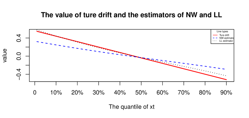
Figure 4: Various Nonparametric Estimators for $\mu(x)=-10*x$ with $T=10,~{}n=1000$ and Variance Gamma jump process $J_{t}$

Table 5: The Biases of Nadaraya-Watson and Local Linear Estimators for $\mu(x)=-10*x$ at various quantile points of sample $X_{t}$ with $T=10,~{}n=1000$ and Variance Gamma jump process $J_{t}$

Bias	Various Quantile Points of Sample Xt
	10%	20%	30%	40%	50%	60%	70%	80%	90%
NW	-0.1702	-0.1088	-0.0564	-0.0178	-0.0110	0.0418	0.0732	0.1045	0.1590
LL	-0.0708	-0.0415	-0.0190	-0.0048	-0.0039	0.0109	0.0152	0.0159	0.0069

Table 6: Simulation results on RMSE-NW and RMSE-LL for three lengths of time interval (T) and three sample sizes for $\mu(x)=-10x$ with Variance Gamma jump process $J_{t}$ over 100 replicates.

Time Span	Estimators	$n=500$	$n=1000$	$n=2500$
$T=10$	RMSE-NW	0.2493	0.1140	0.0962
	RMSE-LL	0.1879	0.0933	0.0494
$T=20$	RMSE-NW	0.4365	0.2481	0.2239
	RMSE-LL	0.2892	0.1564	0.1561
$T=50$	RMSE-NW	1.1106	0.6076	0.2544
	RMSE-LL	0.3077	0.2624	0.1837

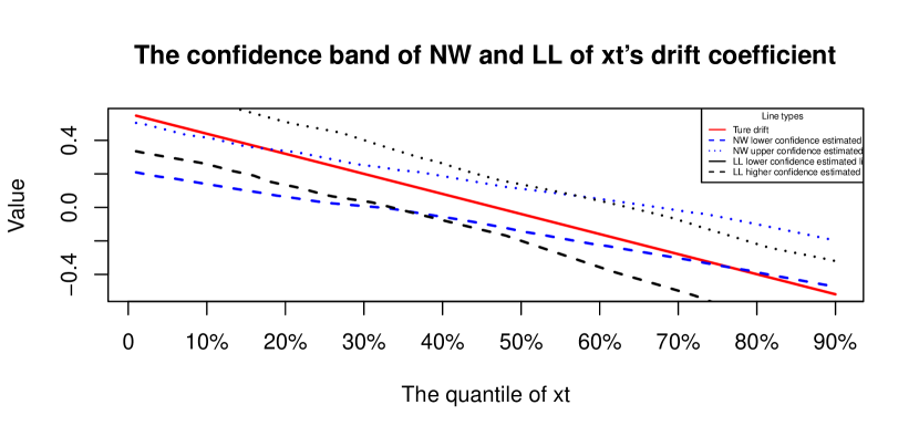
Figure 5: 95% Monte Carlo Confidence Interval for $\mu(x)=-10*x$ with $T=10,~{}n=1000$ and Variance Gamma jump process $J_{t}$

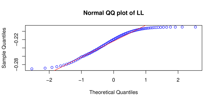
Figure 6: QQ plot of local linear estimator for $\mu(x)=-10*x$ with $T=10,~{}n=1000$ and Variance Gamma jump process $J_{t}$

4 Empirical Analysis

In this section, we apply the integrated diffusion with jump to model the return of stock index from Shenzhen Stock Exchange in China under five-minute high frequency data, that is $\Delta_{n}=\frac{1}{48}$ (t = 1 meaning one day), and then apply the local linear estimators to estimate the unknown coefficients in model (1.2).

We assume that

$$\left\{\begin{array}[]{ll}d\log Y_{t}=X_{t}dt,\\ dX_{t}=\mu(X_{t-})dt+\sigma(X_{t-})dW_{t}+\int_{\mathscr{E}}c(X_{t-},z)r(\omega,dt,dz),\end{array}\right.$$ (4.1)

where $\log Y_{t}$ is the log integrated process for stock index or commodity price and $X_{t}$ is the latent process for the log-returns. According to (2.1), we can get the proxy of the latent process, that is the return of $\log Y_{t}$,

$$\widetilde{X}_{i\Delta_{n}}=\frac{\log Y_{i\Delta_{n}}-\log Y_{(i-1)\Delta_{n}}}{\Delta_{n}}.$$ (4.2)

The plots of Shenzhen Composite Index and its proxy (4.2) under five-minute frequency data from Jan 5, 2015 to Dec 31, 2015 are depicted in Figures 7 and 8. Figure 8 indicates the existence of jumps.

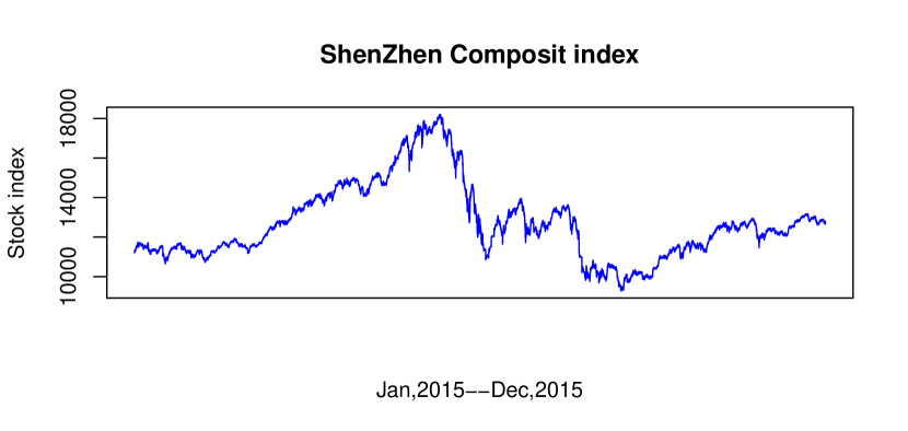
Figure 7: Time Series of Shenzhen Composite Index (2015)

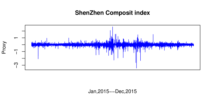
Figure 8: Proxy of Shenzhen Composite Index (2015)

Trough the Augmented Dickey-Fuller test statistic in Table 7, we can easily observe that the null hypothesis of non-stationarity is accepted for the logarithm of stock index $\log Y_{t}$ at the 5% significance level, but is rejected for the difference sequence proxy $X_{t}$, which confirms the stationary Assumption 2 for $X_{t}.$ Furthermore, based on the statistic proposed in Aït-Sahalia and Jacod [1], the degree of activity jumps is 0.3487, which indicates the existence of infinite activity jumps for $X_{t}$ and confirms the validity of model (4.1) with infinite activity jumps for Shenzhen Composite Index.

Table 7: Augmented Dickey-Fuller stationarity test for model

Data		TestStat	CriticalValue	PValue
	$\log Y_{t}$	-1.5298	-2.8610	0.5046
	$X_{t}$	-113.7941	-2.8610	$<0.01$

Here we use Gaussian kernels and the empirical bandwidth $h=1.06*\hat{S}*T^{-1/5}$ for the estimation procedure. The local linear estimators under (4.2) for the unknown coefficients in model (4.1) are displayed in Figures 9 and 10. It is observed that the linear shape with negative coefficient for drift estimator in Figure 9 which reveals the economic phenomenon of mean reversion. It is also shown the quadratic form with positive coefficient for volatility estimator with a minimum at 0.07 in Figure 10, which coincides with the economic phenomenon of volatility smile. The shapes of estimated curves for these unknown coefficients coincide with those in Nicolau [30].

However there is an interesting phenomenon discovered in the volatility line of return series: this line is asymmetric not like the symmetric one in Nicolau [30] and the volatility has different rates to positive return and negative return. The finding coincides with the conclusion in most empirical analysis that asymmetric features are depicted for volatility with respect to positive perturbations (good news) and negative perturbations (bad news). This is statistically due to the higher agglomeration effect of jumps for Shenzhen stock index in 2015. As Johannes [23] pointed out, jumps account for more than half of the conditional variance. Furthermore, as Chen and Sun [6] concluded, the jump behavior has a significant and asymmetric feedback effect in the expected volatility, moreover, jumps exacerbate the degree of asymmetric features of the volatility for stock index. Using the statistics proposed in Aït-Sahalia and Jacod [1], we can observe that at the points of the stock index return which are more than 0.07, jumps happened at approximately 75.50% points in them and at the points of the return which are less than 0.07, jumps happened at about 58.90% points among them. In conclusion, different frequencies of jumps at various points of stock index return lead to the asymmetric volatility line.

What may explain this phenomenon economically is the special situation of stock market in 2015. As we know, Shenzhen index in China performed quite well during first half year of 2015, so more shares changed hands arises for high yield, which leads to higher slope for volatility at larger positive value of log-return increments. However, Shenzhen index performed very unsatisfactorily in the second half year. Facing the big transformation, investors are still immersed in the past prosperity and believe that stocks market crisis is temporary and the market can rebound after hitting rock bottom. Hence less shares changed hands arises, which leads to milder slope for volatility at lower value of log-return increments. From Figure 11, we can observe that more and larger volume happened at positive and large return rate. As a result, investors have different responses to negative and positive returns, which leads to the asymmetric volatility line.

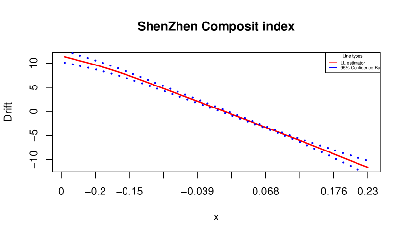
Figure 9: local linear estimator and its 95% confidence bands of the drift coefficient

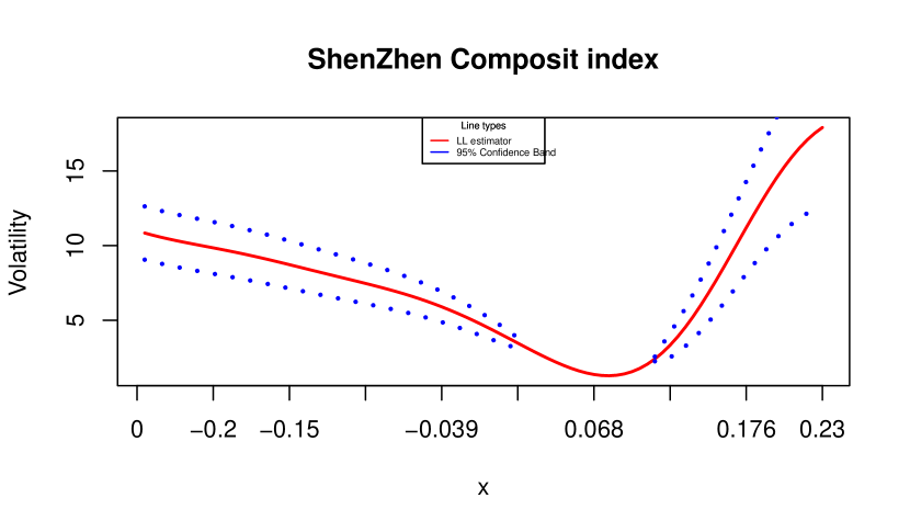
Figure 10: local linear estimator and its 95% confidence bands of the volatility coefficient

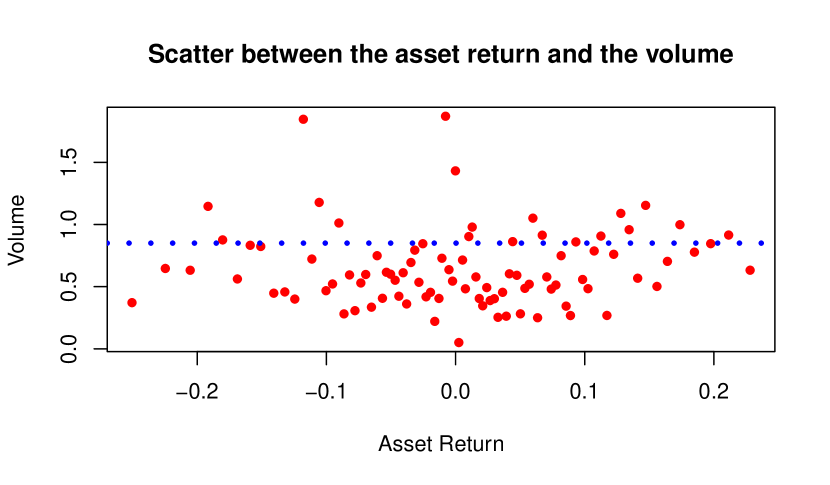
Figure 11: Scatter between the asset return rate and volume

5 Appendix

In this section, we first present some technical lemmas and the proofs for the main theorems.

5.1 Some Technical Lemmas with Proofs

Lemma 1

(Shimizu and Yoshida [33]) Let $Z$ be a $d$-dimensional solution-process to the stochastic differential equation

$$Z_{t}=Z_{0}+\int_{0}^{t}\mu(Z_{s-})ds+\int_{0}^{t}\sigma(Z_{s-})dW_{s}+\int_{0}^{t}\int_{\mathscr{E}}c(Z_{s-},z)r(\omega,dt,dz),$$

where $Z_{0}$ is a random variable, $\mathscr{E}=\mathbb{R}^{d}\setminus\{0\}$, $\mu(x),c(x,z)$ are $d$-dimensional vectors defined on $\mathbb{R}^{d},\mathbb{R}^{d}\times\mathscr{E}$ respectively, $\sigma(x)$ is a $d\times d$ diagnonal matrix defined on $\mathbb{R}^{d}$, and $W_{t}$ is a $d$-dimensional vector of independent Brownian motions.

Let $g$ be a $C^{2(l+1)}$-class function whose derivatives up to 2$(l+1)$th are of polynomial growth. Assume that the coefficient $\mu(x),\sigma(x),$ and $c(x,z)$ are $C^{2l}$-class function whose derivatives with respective to $x$ up to 2$l$th are of polynomial growth. Under Assumption 6, the following expansion holds

$$E[g(Z_{t})|\mathscr{F}_{s}]=\sum_{j=0}^{l}L^{j}g(Z_{s})\frac{\Delta_{n}^{j}}{j!}+R,$$ (5.1)

for $t>s$ and $\Delta_{n}=t-s$, where $R=\int_{0}^{\Delta_{n}}\int_{0}^{u_{1}}\dots\int_{0}^{u_{l}}E[L^{l+1}g(Z_{s+u_{l+1}})|\mathscr{F}_{s}]du_{1}\dots du_{l+1}$ is a stochastic function of order $\Delta_{n}^{l+1},Lg(x)=\partial_{x}^{\ast}g(x)\mu(x)+\frac{1}{2}tr[\partial_{x}^{2}g(x)\sigma(x)\sigma^{\ast}(x)]+\int_{\mathscr{E}}\{g(x+c(x,z))-g(x)-\partial_{x}^{\ast}g(x)c(x,z)\}f(z)dz.$

Remark 5.1

Consider a particularly important model:

$$\left\{\begin{array}[]{ll}dY_{t}=X_{t-}dt,\\ dX_{t}=\mu(X_{t-})dt+\sigma(X_{t-})dW_{t}+\int_{\mathscr{E}}c(X_{t-},z)r(w,dt,dz).\end{array}\right.$$

As $d$ = 2, we have

$$\begin{array}[]{ll}Lg(x,y)=x(\partial g/\partial y)+\mu(x)(\partial g/\partial x)+\frac{1}{2}\sigma^{2}(x)(\partial^{2}g/\partial x^{2})\\ ~{}~{}~{}~{}~{}~{}~{}~{}~{}~{}~{}~{}~{}+\int_{\mathscr{E}}\{g(x+c(x,z),y)-g(x,y)-\frac{\partial g}{\partial x}\cdot c(x,z)\}f(z)dz.\end{array}$$ (5.2)

Based on operator (5.2), one can obtain the equations such as (2.2) and (2.3), one can refer to Appendix A in Song, Lin and Wang [36] for detailed calculations.

Lemma 2

(Jacod [21]) A sequence of $\mathbb{R}-$valued variables $\{\zeta_{n,i}:i\geq 1\}$ defined on the filtered probability space $(\Omega,\mathcal{F},(\mathcal{F})_{t\geq 0},\mathbb{P})$ is $\mathcal{F}_{i\Delta_{n}}-$measurable for all $n,i.$ Assume there exists a continuous adapted $\mathbb{R}-$valued process of finite variation $B_{t}$ and a continuous adapted and increasing process $C_{t}$, for any $t>0,$ we have

$$\sup_{0\leq s\leq t}\big{|}\sum_{i=1}^{[s/\Delta_{n}]}\mathbb{E}\big{[}\zeta_{n,i}|\mathcal{F}_{(i-1)\Delta_{n}}\big{]}-B_{s}\big{|}\stackrel{{\scriptstyle P}}{{\longrightarrow}}0,$$ (5.3)

$$~{}~{}~{}~{}~{}~{}~{}~{}~{}~{}~{}~{}~{}~{}~{}~{}~{}~{}~{}~{}~{}~{}~{}~{}~{}\sum_{i=1}^{[t/\Delta_{n}]}\big{(}\mathbb{E}\big{[}\zeta_{n,i}^{2}|\mathcal{F}_{(i-1)\Delta_{n}}\big{]}-\mathbb{E}^{2}\big{[}\zeta_{n,i}|\mathcal{F}_{(i-1)\Delta_{n}}\big{]}\big{)}-C_{t}\stackrel{{\scriptstyle P}}{{\longrightarrow}}0,$$ (5.4)

$$\sum_{i=1}^{[t/\Delta_{n}]}\mathbb{E}\big{[}\zeta_{n,i}^{4}|\mathcal{F}_{(i-1)\Delta_{n}}\big{]}\stackrel{{\scriptstyle P}}{{\longrightarrow}}0.$$ (5.5)

Then the processes

$$\sum_{i=1}^{[t/\Delta_{n}]}\zeta_{n,i}\Rightarrow B_{t}+M_{t},$$

where $M_{t}$ is a continuous process defined on the filtered probability space $\big{(}{\Omega},{P},{\mathcal{F}}\big{)}$ and which, conditionally on the the $\sigma-$filter $\mathcal{F}$, is a centered Gaussian $\mathbb{R}-$valued process with $E\big{[}M_{t}^{2}|\mathcal{F}\big{]}=C_{t}.$

Remark 5.2

Condition (5.5) is a conditional Lindeberg theorem or Lyapounov's condition, whose aims is to ensure that the limiting process is continuous. It is a particular case of Theorem IX.7.28 in Jacod and Shiryaev [22].

Lemma 3

(Song, Lin [37]) Under Assumptions 1 - 5, we have

$$\frac{1}{nh_{n}}\sum_{i=1}^{n}K\left(\frac{X_{i}-x}{h_{n}}\right)\left(\frac{X_{i}-x}{h_{n}}\right)^{k}~{}\stackrel{{\scriptstyle\mathrm{a.s.}}}{{\longrightarrow}}~{}p(x)K_{1}^{k},$$ (5.6)

where $K_{1}^{k}:=\int u^{k}K(u)du.$

Remark 5.3

We can obtain that

$$\frac{1}{nh_{n}^{3}}\sum_{j=1}^{n}K\left(\frac{X_{j-1}-x}{h_{n}}\right)(X_{j-1}-x)^{2}\stackrel{{\scriptstyle\mathrm{a.s.}}}{{\longrightarrow}}~{}p(x)K_{1}^{2},$$ (5.7)

and

$$\frac{1}{nh_{n}^{2}}\sum_{j=1}^{n}K\left(\frac{X_{j-1}-x}{h_{n}}\right)(X_{j-1}-x)\stackrel{{\scriptstyle\mathrm{a.s.}}}{{\longrightarrow}}~{}p(x)K_{1}^{1}.$$ (5.8)

Lemma 4

Under Assumptions 1- 5, let

$$\mu_{n}^{\ast}(x)=\frac{\sum_{i=1}^{n}w_{i-1}^{\ast}\left(\frac{X_{i}-X_{i-1}}{\Delta_{n}}\right)}{\sum_{i=1}^{n}w_{i-1}^{\ast}}$$

and

$$M_{n}^{\ast}(x)=\frac{\sum_{i=1}^{n}w_{i-1}^{\ast}\frac{(X_{i}-X_{i-1})^{2}}{\Delta_{n}}}{\sum_{i=1}^{n}w_{i-1}^{\ast}}.$$

where

$$w_{i}^{\ast}=K\left(\frac{X_{i}-x}{h_{n}}\right)\left(\sum_{j=1}^{n}K\left(\frac{X_{j-1}-x}{h_{n}}\right)(X_{j-1}-x)^{2}-(X_{i}-x)\sum_{j=1}^{n}K\left(\frac{X_{j-1}-x}{h_{n}}\right)(X_{j-1}-x)\right)$$

then

$$\mu_{n}^{\ast}(x)\stackrel{{\scriptstyle p}}{{\rightarrow}}\mu(x),~{}~{}~{}M_{n}^{\ast}(x)\stackrel{{\scriptstyle p}}{{\rightarrow}}M(x).$$

Furthermore, if $h_{n}n\Delta_{n}\longrightarrow 0$ and $h_{n}=O((n\Delta_{n})^{-1/5}),$ then

$$\sqrt{h_{n}n\Delta_{n}}\left(\mu_{n}^{\ast}(x)-\mu(x)-\frac{1}{2}h_{n}^{2}\mu^{{}^{\prime\prime}}(x)\frac{(K_{1}^{2})^{2}-K_{1}^{3}K_{1}^{1}}{K_{1}^{2}-(K_{1}^{1})^{2}}\right)\Longrightarrow N\left(0,V\frac{M(x)}{p(x)}\right),$$

and

$$\sqrt{h_{n}n\Delta_{n}}\left(M_{n}^{\ast}(x)-M(x)-\frac{1}{2}h_{n}^{2}M^{{}^{\prime\prime}}(x)\frac{(K_{1}^{2})^{2}-K_{1}^{3}K_{1}^{1}}{K_{1}^{2}-(K_{1}^{1})^{2}}\right)\Longrightarrow N\left(0,V\frac{\int_{\mathscr{E}}c^{4}(x,y)\nu(dy)}{p(x)}\right),$$

where

$$V=\frac{(K_{1}^{2})^{2}K_{2}^{0}+(K_{1}^{1})^{2}K_{2}^{2}-2(K_{1}^{1})(K_{1}^{2})K_{2}^{1}}{[K_{1}^{2}-(K_{1}^{1})^{2}]^{2}}.$$

Remark 5.4

The main method to obtain the asymptotic properties for estimator of model (1.2) is to approximate the estimator for (1.2) by the similar estimator for univariate jump-diffusion $X_{t}$ in probability. Based on the basic idea, we should first know the asymptotic properties for the local linear estimator for univariate jump-diffusion $X_{t}$ before the Theorems 2.6 presented. Lemma 4 gives us the desired properties for local linear estimator for univariate jump-diffusion $X_{t}.$

• Proof. As for the finite activity jumps case of $X_{t},$ Hanif [18], Chen and Zhang [7] considered the weak consistency and asymptotic normality for the estimators $\mu_{n}^{\ast}(x)$ and $M_{n}^{\ast}(x).$ Song, Lin [37] discussed the weak consistency and asymptotic normality of $\mu_{n}^{\ast}(x)$ for the infinite activity jumps case of $X_{t}.$ They also derived the weak consistency of $M_{n}^{\ast}(x)$ for the asymptotic variance of the asymptotic distribution of $\mu_{n}^{\ast}(x).$ However, they did not study the asymptotic distribution of $M_{n}^{\ast}(x)$ for the infinite activity jumps case which we will give a detailed proof for based on the Lemma 3.

  Using Itô formula to the jump-diffusion setting shown in Protter [32], we can write

  $$(X_{(i+1)\Delta_{n}}-X_{i\Delta_{n}})^{2}$$

  $$= 2\int_{i\Delta_{n}}^{(i+1)\Delta_{n}}(X_{s-}-X_{i\Delta_{n}})\mu(X_{s-})ds+2\int_{i\Delta_{n}}^{(i+1)\Delta_{n}}(X_{s-}-X_{i\Delta_{n}})\sigma(X_{s-})dW_{s}$$

  $$+2\int_{i\Delta_{n}}^{(i+1)\Delta_{n}}(X_{s-}-X_{i\Delta_{n}})\xi(X_{s-})dJ_{s}+\int_{i\Delta_{n}}^{(i+1)\Delta_{n}}(\sigma^{2}(X_{s-})+\xi^{2}(X_{s-})Var(J(1)))ds$$

  $$+\int_{i\Delta_{n}}^{(i+1)\Delta_{n}}\xi^{2}(X_{s-})\int_{\mathbb{R}}y^{2}\bar{\mu}(dy,ds).$$

  Hence we can derive that

  $$M_{n}^{\ast}(x)-M(x)$$

  $$= \frac{\frac{1}{n^{2}h_{n}^{4}}\sum_{i=1}^{n}w_{i-1}^{\ast}\left((X_{i}-X_{i-1})^{2}-M(x)\cdot\Delta_{n}\right)}{\frac{\Delta_{n}}{n^{2}h_{n}^{4}}\sum_{i=1}^{n}w_{i-1}^{\ast}}$$

  $$= \frac{1}{\frac{\Delta_{n}}{n^{2}h_{n}^{4}}\sum_{i=1}^{n}w_{i-1}^{\ast}}*\frac{1}{n^{2}h_{n}^{4}}\sum_{i=1}^{n}w_{i-1}^{\ast}\Bigg{\{}\left[\int_{(i-1)\Delta_{n}}^{i\Delta_{n}}(\sigma^{2}(X_{s-})+\xi^{2}(X_{s-})Var(J(1)))ds-M(x)\cdot\Delta_{n}\right]$$

  $$+\left[2\int_{(i-1)\Delta_{n}}^{i\Delta_{n}}(X_{s-}-X_{i\Delta_{n}})\mu(X_{s-})ds\right]+\left[2\int_{(i-1)\Delta_{n}}^{i\Delta_{n}}(X_{s-}-X_{i\Delta_{n}})\sigma(X_{s-})dW_{s}\right]$$

  $$+\left[2\int_{(i-1)\Delta_{n}}^{i\Delta_{n}}(X_{s-}-X_{i\Delta_{n}})\xi(X_{s-})dJ_{s}\right]+\left[\int_{(i-1)\Delta_{n}}^{i\Delta_{n}}\xi^{2}(X_{s-})\int_{\mathbb{R}}y^{2}\bar{\mu}(dy,ds)\right]\Bigg{\}}$$

  $$=: b_{1_{n}}+A_{2_{n}}+A_{3_{n}}+A_{4_{n}}+A_{5_{n}}.$$

  We can express $b_{1_{n}},$ which dominates the bias for the estimator of $M_{n}^{\ast}(x),$ as

  $$b_{1_{n}} = \frac{1}{\frac{\Delta_{n}}{n^{2}h_{n}^{4}}\sum_{i=1}^{n}w_{i-1}^{\ast}}*\frac{1}{n^{2}h_{n}^{4}}\sum_{i=1}^{n}w_{i-1}^{\ast}\int_{(i-1)\Delta_{n}}^{i\Delta_{n}}(M(X_{s-})-M(x))ds$$

  $$= \frac{1}{\frac{\Delta_{n}}{n^{2}h_{n}^{4}}\sum_{i=1}^{n}w_{i-1}^{\ast}}*\frac{1}{n^{2}h_{n}^{4}}\sum_{i=1}^{n}w_{i-1}^{\ast}\int_{(i-1)\Delta_{n}}^{i\Delta_{n}}(M(X_{s-})-M(X_{(i-1)\Delta_{n}}))ds$$

  $$+\frac{1}{\frac{1}{n^{2}h_{n}^{4}}\sum_{i=1}^{n}w_{i-1}^{\ast}}*\frac{1}{n^{2}h_{n}^{4}}\sum_{i=1}^{n}w_{i-1}^{\ast}(M(X_{(i-1)\Delta_{n}})-M(x))$$

  $$= \frac{1}{\frac{\Delta_{n}}{n^{2}h_{n}^{4}}\sum_{i=1}^{n}w_{i-1}^{\ast}}*\frac{1}{n^{2}h_{n}^{4}}\sum_{i=1}^{n}w_{i-1}^{\ast}\int_{(i-1)\Delta_{n}}^{i\Delta_{n}}(X_{s-}-X_{(i-1)\Delta_{n}})M^{{}^{\prime}}(\tilde{X}_{s-})ds$$

  $$+\frac{1}{\frac{1}{n^{2}h_{n}^{4}}\sum_{i=1}^{n}w_{i-1}^{\ast}}*\frac{1}{n^{2}h_{n}^{4}}\sum_{i=1}^{n}w_{i-1}^{\ast}[M^{{}^{\prime}}(x)(X_{(i-1)\Delta_{n}}-x)+\frac{1}{2}M^{{}^{\prime\prime}}(\hat{X}_{s-})(X_{(i-1)\Delta_{n}}-x)^{2}],$$

  where $\tilde{X}_{s-}$ lies between $X_{s-}$ and $X_{(i-1)\Delta_{n}},$ $\hat{X}_{s-}$ lies between $X_{(i-1)\Delta_{n}}$ and $x.$

  Under a simple calculus, we have

  $$\sum_{i=1}^{n}w_{i-1}^{\ast}(X_{(i-1)\Delta_{n}}-x)\equiv 0,$$ (5.9)

  so we can obtain that

  $$b_{1_{n}} = \frac{1}{\frac{\Delta_{n}}{n^{2}h_{n}^{4}}\sum_{i=1}^{n}w_{i-1}^{\ast}}*\frac{1}{n^{2}h_{n}^{4}}\sum_{i=1}^{n}w_{i-1}^{\ast}\int_{(i-1)\Delta_{n}}^{i\Delta_{n}}(X_{s-}-X_{(i-1)\Delta_{n}})M^{{}^{\prime}}(\tilde{X}_{s-})ds$$

  $$+\frac{1}{2}\frac{1}{\frac{1}{n^{2}h_{n}^{4}}\sum_{i=1}^{n}w_{i-1}^{\ast}}*\frac{1}{n^{2}h_{n}^{4}}\sum_{i=1}^{n}w_{i-1}^{\ast}M^{{}^{\prime\prime}}(\hat{X}_{s-})(X_{(i-1)\Delta_{n}}-x)^{2}$$

  $$=: b_{11_{n}}+b_{12_{n}}.$$

  Now, define

  $$\delta_{n,T}=\max_{i\leq n}\sup_{i\Delta_{n}\leq s\leq(i+1)\Delta_{n}}\left|X_{s-}-X_{i\Delta_{n}}\right|.$$

  Using the similar procedure as Bandi and Nguyen [2], one can have

  $$\varlimsup_{n\rightarrow\infty}{\frac{\delta_{n,T}}{\left(\Delta_{n}\log(1/\Delta_{n})\right)^{1/2}}}=C_{1}~{}~{}~{}~{}~{}~{}a.s.$$ (5.10)

  for some constant $C_{1},$ which implies that $\delta_{n,T}=o_{a.s.}(1).$

  It follows from the similar procedure of Lemma 3 as that in Song, Lin [37] for the numerator of $b_{12_{n}}$ with the equation (5.10)

  $$\frac{1}{h_{n}^{2}}b^{Num}_{12_{n}}\stackrel{{\scriptstyle\mathrm{a.s.}}}{{\longrightarrow}}\frac{1}{2}p^{2}(x)M^{{}^{\prime\prime}}(x)\left[(K_{1}^{2})^{2}-K_{1}^{3}K_{1}^{1}\right].$$ (5.11)

  With the asymptotic equations in Remark 5.3, we can easily get for the denominator of $b_{12_{n}}$

  $$b^{Den}_{12_{n}}=\frac{1}{n^{2}h_{n}^{4}}\sum_{i=1}^{n}w_{i-1}^{\ast}\stackrel{{\scriptstyle\mathrm{a.s.}}}{{\longrightarrow}}p^{2}(x)\left[K_{1}^{2}-(K_{1}^{1})^{2}\right].$$ (5.12)

  Using the property that if $\xi_{n}\stackrel{{\scriptstyle P}}{{\rightarrow}}\xi$ and $\eta_{n}\rightarrow c$ where $c$ is a nonzero constant, then $\xi_{n}/\eta_{n}\stackrel{{\scriptstyle P}}{{\rightarrow}}\xi/c,$ we have

  $$\frac{1}{h_{n}^{2}}b_{12_{n}}\stackrel{{\scriptstyle P}}{{\longrightarrow}}\frac{1}{2}M^{{}^{\prime\prime}}(x)\frac{(K_{1}^{2})^{2}-K_{1}^{3}K_{1}^{1}}{K_{1}^{2}-(K_{1}^{1})^{2}}.$$ (5.13)

  $b_{11_{n}}$ and $A_{2_{n}}$ can be dealt with the similar proof procedure, here we only consider $A_{2_{n}}.$ Based on the equation (5.10), the asymptotic equations in Remark 5.3 and Assumption 5, we have that

  $$A_{2_{n}}=\left(\Delta_{n}\log(1/\Delta_{n})\right)^{1/2}O_{a.s.}(1)=o_{p}(b_{12_{n}}).$$ (5.14)

  Note that

  $$A_{3_{n}}=\left(\Delta_{n}\log(1/\Delta_{n})\right)^{1/2}O_{p}(A_{5_{n}})=o_{p}(A_{5_{n}}),$$ (5.15)

  and

  $$A_{4_{n}}=\left(\Delta_{n}\log(1/\Delta_{n})\right)^{1/2}O_{p}(A_{5_{n}})=o_{p}(A_{5_{n}}),$$ (5.16)

  which implies that $A_{5_{n}}$ is responsible for the asymptotic distribution.

  Now we only focus on the examination of the term $A_{5_{n}}.$ Denote that

  $$w_{i}^{{\dagger}}=K\left(\frac{X_{i}-x}{h_{n}}\right)\left(K_{1}^{2}-\left(\frac{X_{i}-x}{h_{n}}\right)K_{1}^{1}\right),$$ (5.17)

  and

  $$\frac{\sqrt{h_{n}n\Delta_{n}}}{nh_{n}\Delta_{n}}\sum_{i=1}^{n}w_{i-1}^{{\dagger}}\int_{(i-1)\Delta_{n}}^{i\Delta_{n}}\xi^{2}(X_{s-})\int_{\mathbb{R}}y^{2}\bar{\mu}(dy,ds):=\sum_{i=1}^{n}q_{i}.$$ (5.18)

  We can obtain that $\sum_{i=1}^{n}q_{i}\stackrel{{\scriptstyle D}}{{\longrightarrow}}N(0,[(K_{1}^{2})^{2}K_{2}^{0}-2K_{1}^{1}K_{1}^{2}K_{2}^{1}+(K_{1}^{1})^{2}K_{2}^{2}]\xi^{4}(x)\int_{\mathbb{R}}y^{4}\nu(dy)p(x))$ by Lemma 2, if the following conditions hold

  $|S_{1}|=\big{|}\sum_{i=1}^{n}E_{i-1}[q_{i}]\big{|}\stackrel{{\scriptstyle P}}{{\rightarrow}}0;$

  $S_{2}=\sum_{i=1}^{n}\big{(}E_{i-1}[{q_{i}}^{2}]-E_{i}^{2}[q_{1,i+1}]\big{)}\stackrel{{\scriptstyle P}}{{\longrightarrow}}[(K_{1}^{2})^{2}K_{2}^{0}-2K_{1}^{1}K_{1}^{2}K_{2}^{1}+(K_{1}^{1})^{2}K_{2}^{2}]\xi^{4}(x)\int_{\mathbb{R}}y^{4}\nu(dy)p(x);$

  $S_{3}=\sum_{i=1}^{n}E_{i-1}[{q_{i}}^{4}]\stackrel{{\scriptstyle P}}{{\rightarrow}}0;$

  where $E_{i-1}[~{}\cdot~{}]=E[~{}\cdot~{}|X_{(i-1)\Delta_{n}}]$ and $q_{i}$ is $\mathcal{F}_{i\Delta_{n}}-$measurable, which is the $\sigma-$algebra generated by $\{X_{j\Delta_{n}},~{}j\leq i\}.$

  For $S_{2},$ the asymptotic variance can analogously be derived as the drift case in Funke [12] by replacing $K\left(\frac{X_{i}-x}{h_{n}}\right)$ with $w_{i}^{{\dagger}},$ $\xi(X_{s-})$ with $\xi^{2}(X_{s-})$ and $dL_{t}=\int_{\mathbb{R}}y\bar{\mu}(dy,ds)$ with $\int_{\mathbb{R}}y^{2}\bar{\mu}(dy,ds).$

  For $|S_{1}|,$ since

  $$E_{i-1}[q_{i}] = \frac{1}{\sqrt{h_{n}n\Delta_{n}}}w_{i-1}^{{\dagger}}E_{i-1}\left[\int_{(i-1)\Delta_{n}}^{i\Delta_{n}}\xi^{2}(X_{s-})\int_{\mathbb{R}}y^{2}\bar{\mu}(dy,ds)\right]$$

  $$\equiv 0,$$

  we can get $|S_{1}|\equiv 0.$

  For $S_{3},$ with BDG inequality we obtain that

  $$\sum_{i=1}^{n}E_{i-1}[{q_{i}}^{4}]$$

  $$= \frac{1}{(nh_{n}\Delta_{n})^{2}}\sum_{i=1}^{n}w_{i-1}^{{\dagger}4}E_{i-1}\left[\left(\int_{(i-1)\Delta_{n}}^{i\Delta_{n}}\xi^{2}(X_{s-})\int_{\mathbb{R}}y^{2}\bar{\mu}(dy,ds)\right)^{4}\right]$$

  $$\leq C\frac{n}{(nh_{n}\Delta_{n})^{2}}(\Delta_{n}^{2}+\Delta_{n})$$

  $$= C\frac{1}{nh^{2}_{n}}+C\frac{1}{n\Delta_{n}h^{2}_{n}}\rightarrow 0.$$

  Furthermore, we can obtain

  $$\frac{\sqrt{h_{n}n\Delta_{n}}}{n^{2}h_{n}^{4}\Delta_{n}}\sum_{i=1}^{n}w_{i-1}^{\ast}\int_{(i-1)\Delta_{n}}^{i\Delta_{n}}\xi^{2}(X_{s-})\int_{\mathbb{R}}y^{2}\bar{\mu}(dy,ds)$$

  $$- \frac{\sqrt{h_{n}n\Delta_{n}}}{nh_{n}\Delta_{n}}\sum_{i=1}^{n}w_{i-1}^{{\dagger}}\int_{(i-1)\Delta_{n}}^{i\Delta_{n}}\xi^{2}(X_{s-})\int_{\mathbb{R}}y^{2}\bar{\mu}(dy,ds)$$

  $$= \left(\frac{1}{nh_{n}^{3}}\sum_{j=1}^{n}K\left(\frac{X_{j-1}-x}{h_{n}}\right)(X_{j-1}-x)^{2}-K_{1}^{2}\right)\times$$

  $$\times\frac{1}{\sqrt{h_{n}n\Delta_{n}}}\sum_{i=1}^{n}K\left(\frac{X_{i}-x}{h_{n}}\right)\int_{(i-1)\Delta_{n}}^{i\Delta_{n}}\xi^{2}(X_{s-})\int_{\mathbb{R}}y^{2}\bar{\mu}(dy,ds)$$

  $$-\left(\frac{1}{nh_{n}^{2}}K\left(\frac{X_{j-1}-x}{h_{n}}\right)(X_{j-1}-x)-K_{1}^{1}\right)\times$$

  $$\times\frac{1}{\sqrt{h_{n}n\Delta_{n}}}\sum_{i=1}^{n}K\left(\frac{X_{i}-x}{h_{n}}\right)\left(\frac{X_{i}-x}{h_{n}}\right)\int_{(i-1)\Delta_{n}}^{i\Delta_{n}}\xi^{2}(X_{s-})\int_{\mathbb{R}}y^{2}\bar{\mu}(dy,ds)$$

  $$=: \left(\frac{1}{nh_{n}^{3}}\sum_{j=1}^{n}K\left(\frac{X_{j-1}-x}{h_{n}}\right)(X_{j-1}-x)^{2}-K_{1}^{2}\right)\sum_{i=1}^{n}q_{i}^{{}^{\prime}}$$

  $$-\left(\frac{1}{nh_{n}^{2}}K\left(\frac{X_{j-1}-x}{h_{n}}\right)(X_{j-1}-x)-K_{1}^{1}\right)\sum_{i=1}^{n}q_{i}^{{}^{\prime\prime}}.$$

  Under the same proof procedure as $\sum_{i=1}^{n}q_{i},$ we can prove that $\sum_{i=1}^{n}q_{i}^{{}^{\prime}}\stackrel{{\scriptstyle D}}{{\longrightarrow}}N(0,K_{2}^{0}\xi^{4}(x)\int_{\mathbb{R}}y^{4}\nu(dy)p(x))$ and $\sum_{i=1}^{n}q_{i}^{{}^{\prime\prime}}\stackrel{{\scriptstyle D}}{{\longrightarrow}}N(0,K_{2}^{2}\xi^{4}(x)\int_{\mathbb{R}}y^{4}\nu(dy)p(x)),$ which implies that $\sum_{i=1}^{n}q_{i}^{{}^{\prime}}=O_{p}(1)$ and $\sum_{i=1}^{n}q_{i}^{{}^{\prime\prime}}=O_{p}(1).$ Hence with the Remark 5.3 we can obtain

  $$\frac{\sqrt{h_{n}n\Delta_{n}}}{n^{2}h_{n}^{4}\Delta_{n}}\sum_{i=1}^{n}w_{i-1}^{\ast}\int_{(i-1)\Delta_{n}}^{i\Delta_{n}}\xi^{2}(X_{s-})\int_{\mathbb{R}}y^{2}\bar{\mu}(dy,ds)$$

  $$- \frac{\sqrt{h_{n}n\Delta_{n}}}{nh_{n}\Delta_{n}}\sum_{i=1}^{n}w_{i-1}^{{\dagger}}\int_{(i-1)\Delta_{n}}^{i\Delta_{n}}\xi^{2}(X_{s-})\int_{\mathbb{R}}y^{2}\bar{\mu}(dy,ds)=o_{p}(1).$$

  By the Slutsky's theorem, we can get that

  $$\frac{\sqrt{h_{n}n\Delta_{n}}}{n^{2}h_{n}^{4}\Delta_{n}}\sum_{i=1}^{n}w_{i-1}^{\ast}\int_{(i-1)\Delta_{n}}^{i\Delta_{n}}\xi^{2}(X_{s-})\int_{\mathbb{R}}y^{2}\bar{\mu}(dy,ds)$$

  $$\stackrel{{\scriptstyle D}}{{\longrightarrow}} N(0,[(K_{1}^{2})^{2}K_{2}^{0}-2K_{1}^{1}K_{1}^{2}K_{2}^{1}+(K_{1}^{1})^{2}K_{2}^{2}]\xi^{4}(x)\int_{\mathbb{R}}y^{4}\nu(dy)p(x))$$

  Using the property that if $\xi_{n}\stackrel{{\scriptstyle D}}{{\rightarrow}}\xi$ and $\eta_{n}\stackrel{{\scriptstyle P}}{{\rightarrow}}c$ where $c$ is a nonzero constant, then $\xi_{n}/\eta_{n}\stackrel{{\scriptstyle P}}{{\rightarrow}}\xi/c,$ we have proved the asymptotic distribution of $M_{n}^{\ast}(x)$

  $$\sqrt{h_{n}n\Delta_{n}}\left(M_{n}^{\ast}(x)-M(x)-\frac{1}{2}h_{n}^{2}M^{{}^{\prime\prime}}(x)\frac{(K_{1}^{2})^{2}-K_{1}^{3}K_{1}^{1}}{K_{1}^{2}-(K_{1}^{1})^{2}}\right)\Longrightarrow N\left(0,V\frac{\xi^{4}(x)\int_{\mathbb{R}}y^{4}\nu(dy)}{p(x)}\right),$$ (5.19)

  where $V=\frac{(K_{1}^{2})^{2}K_{2}^{0}+(K_{1}^{1})^{2}K_{2}^{2}-2(K_{1}^{1})(K_{1}^{2})K_{2}^{1}}{[K_{1}^{2}-(K_{1}^{1})^{2}]^{2}}.$

5.2 The proof of Theorem 2.6

• Proof. As for the finite activity jumps case of $X_{t},$ Chen and Zhang [7] considered the weak consistency and asymptotic normality of the estimators $\hat{\mu}_{n}(x)$ and $\hat{M}_{n}(x)$ for the second-order jump-diffusion. Here we will give a detailed proof for the second-order diffusion with infinite activity jumps. For simplicity, here we only prove the results for $\hat{\mu}_{n}(x)$ and one can take the similar proof procedure for $\hat{M}_{n}(x).$

  Weak Consistency: By Lemma 4, it suffices to show that :

  $$\hat{\mu}_{n}(x)-\mu^{\ast}_{n}(x)\stackrel{{\scriptstyle p}}{{\rightarrow}}0.$$

  Firstly, we prove that

  $$\frac{1}{n^{2}h_{n}^{4}}\sum_{i=1}^{n}w_{i-1}-\frac{1}{n^{2}h_{n}^{4}}\sum_{i=1}^{n}w_{i-1}^{\ast}\stackrel{{\scriptstyle p}}{{\rightarrow}}0.$$ (5.20)

  To this end, we should prove that

  $$\frac{1}{nh_{n}}\sum_{i=1}^{n}K\left(\frac{\tilde{X}_{i-1}-x}{h_{n}}\right)-\frac{1}{nh_{n}}\sum_{i=1}^{n}K\left(\frac{X_{i-1}-x}{h_{n}}\right)\stackrel{{\scriptstyle p}}{{\rightarrow}}0,$$ (5.21)

  $$\frac{1}{nh_{n}^{2}}\sum_{i=1}^{n}K\left(\frac{\tilde{X}_{i-1}-x}{h_{n}}\right)(\tilde{X}_{i}-x)-\frac{1}{nh_{n}^{2}}\sum_{i=1}^{n}K\left(\frac{X_{i-1}-x}{h_{n}}\right)(X_{i-1}-x)\stackrel{{\scriptstyle p}}{{\rightarrow}}0,$$ (5.22)

  $$\frac{1}{nh_{n}^{3}}\sum_{i=1}^{n}K\left(\frac{\tilde{X}_{i-1}-x}{h_{n}}\right)(\tilde{X}_{i}-x)^{2}-\frac{1}{nh_{n}^{3}}\sum_{i=1}^{n}K\left(\frac{X_{i-1}-x}{h_{n}}\right)(X_{i-1}-x)^{2}\stackrel{{\scriptstyle p}}{{\rightarrow}}0.$$ (5.23)

  For (5.21), let $\varepsilon_{1,n}=\frac{1}{nh_{n}}\sum_{i=1}^{n}K\left(\frac{\tilde{X}_{i-1}-x}{h_{n}}\right)-\frac{1}{nh_{n}}\sum_{i=1}^{n}K\left(\frac{X_{i-1}-x}{h_{n}}\right).$

  By the mean-value theorem, stationarity, Assumptions 3, 5 and (5.10), we obtain

  $$E[|\varepsilon_{1,n}|] \leq E\left[\frac{1}{nh_{n}}\sum_{i=1}^{n}|K^{{}^{\prime}}(\xi_{n,i})\frac{\widetilde{X}_{(i-1)\Delta_{n}}-{X}_{(i-1)\Delta_{n}}}{h_{n}}|\right]$$

  $$= E\left[\frac{1}{h_{n}}|K^{{}^{\prime}}(\xi_{n,2})\frac{\widetilde{X}_{\Delta_{n}}-{X}_{\Delta_{n}}}{h_{n}}|\right]$$

  $$\leq {\frac{\sqrt{\Delta_{n}\log(1/\Delta_{n})}}{h_{n}}E\left[\frac{1}{h_{n}}|K^{{}^{\prime}}(\xi_{n,2})|\right]\rightarrow 0},$$

  where $\xi_{n,2}$ = $\theta(\frac{x-X_{\Delta_{n}}}{h})+(1-\theta)(\frac{x-\widetilde{X}_{\Delta_{n}}}{h})~{}0\leq\theta\leq 1.$ Hence, (5.21) follows from Chebyshev's inequality.

  For (5.22) we should prove that

  $$\delta_{1,n}=\frac{1}{nh_{n}^{2}}\sum_{i=1}^{n}K\left(\frac{\tilde{X}_{i-1}-x}{h_{n}}\right)(\tilde{X}_{i}-x)-\frac{1}{nh_{n}^{2}}\sum_{i=1}^{n}K\left(\frac{{X}_{i-1}-x}{h_{n}}\right)(\tilde{X}_{i}-x)\stackrel{{\scriptstyle p}}{{\rightarrow}}0,$$ (5.24)

  and

  $$\delta_{2,n}=\frac{1}{nh_{n}^{2}}\sum_{i=1}^{n}K\left(\frac{{X}_{i-1}-x}{h_{n}}\right)(\tilde{X}_{i}-x)-\frac{1}{nh_{n}^{2}}\sum_{i=1}^{n}K\left(\frac{{X}_{i-1}-x}{h_{n}}\right)({X}_{i-1}-x)\stackrel{{\scriptstyle p}}{{\rightarrow}}0.$$ (5.25)

  Under Assumptions 3 and 5, we have

  $$\big{|}E[\delta_{1,n}]\big{|} = \left|E\left[\frac{1}{nh_{n}^{2}}\sum_{i=1}^{n}\left\{K\left(\frac{\tilde{X}_{i-1}-x}{h_{n}}\right)-K\left(\frac{{X}_{i-1}-x}{h_{n}}\right)\right\}(\tilde{X}_{i}-x)\right]\right|$$

  $$= \frac{1}{h_{n}^{2}}\left|E\left[\left\{K\left(\frac{\tilde{X}_{i-1}-x}{h_{n}}\right)-K\left(\frac{{X}_{i-1}-x}{h_{n}}\right)\right\}E[\tilde{X}_{i}-x\big{|}\mathscr{F}_{i-1}]\right]\right|$$

  $$= \frac{1}{h_{n}^{2}}\left|E[K^{\prime}(\xi_{n,i})\frac{(\tilde{X}_{i-1}-X_{i-1})}{h_{n}}(X_{i-1}-x+O_{P}(\Delta_{n}))]\right|$$

  $$\leq \frac{\sqrt{\Delta_{n}\log(1/\Delta_{n})}}{h_{n}^{2}}E[\frac{1}{h_{n}}|K^{\prime}(\xi_{n,i})(X_{i-1}-x+O_{P}(\Delta_{n}))|]$$

  $$\rightarrow 0,$$

  by stationarity, the mean-value theorem and Remark 5.1. So $E[\delta_{1,n}]\rightarrow 0.$

  If we can prove $Var[\delta_{1,n}]\rightarrow 0$, then (5.24) holds. Now we calculate $Var[\delta_{1,n}]$

  $$Var[\delta_{1,n}] = \frac{1}{nh_{n}}Var[\frac{1}{\sqrt{n}}\sum_{i=1}^{n}\frac{1}{h_{n}^{3/2}}K^{{}^{\prime}}(\xi_{n,i})\frac{\widetilde{X}_{i-1}-X_{i-1}}{h_{n}}(\widetilde{X}_{i}-x)]$$

  $$=: \frac{1}{nh_{n}}Var[\frac{1}{\sqrt{n}}\sum_{i=1}^{n}f_{i}].$$

  where $f_{i}:=\frac{1}{h_{n}^{3/2}}K^{{}^{\prime}}(\xi_{n,i})\frac{\widetilde{X}_{i-1}-X_{i-1}}{h_{n}}(\widetilde{X}_{i}-x).$

  By Remark 5.1 and Assumptions 3 and 5, we get

  $$E[f_{i}^{2}] = E\left[\frac{1}{h_{n}^{3}}K^{{}^{\prime}2}(\xi_{n,i})\frac{(\widetilde{X}_{i-1}-X_{i-1})^{2}}{h^{2}_{n}}E[(\widetilde{X}_{i}-x)^{2}|\mathscr{F}_{i-1}]\right]$$

  $$\leq \frac{\Delta_{n}\log(1/\Delta_{n})}{h^{2}_{n}}E\left[\frac{1}{h_{n}^{3}}K^{{}^{\prime}2}(\xi_{n,i})((X_{i}-x)^{2}+O_{p}(\Delta_{n}))\right]$$

  $$< \infty$$

  We notice that $f_{i}$ is stationary under Assumption 2 and $\rho$-mixing with the same size as process $\{\tilde{X}_{i\Delta_{n}};i=1,2,...\}$ and $\{X_{i\Delta_{n}};i=1,2,...\}$. So from Lemma 10.1.c with p=q=2 in Lin and Bai([25], p. 132), we have

  $$\big{|}Var[\frac{1}{\sqrt{n}}\sum_{i=1}^{n}f_{i}]\big{|} = \big{|}\frac{1}{n}[\sum_{i=1}^{n}Var(f_{i})+2\sum_{j=1}^{n-1}\sum_{i=j+1}^{n}(Ef_{i}f_{j}-Ef_{i}Ef_{j})]\big{|}$$

  $$= Var(f_{i})+\frac{2}{n}\big{|}\sum_{j=1}^{n-1}\sum_{i=j+1}^{n}(Ef_{i}f_{j}-Ef_{i}Ef_{j})]\big{|}$$

  $$\leq Var(f_{i})+\frac{2}{n}\sum_{j=1}^{n-1}\sum_{i=j+1}^{n}\big{|}Ef_{i}f_{j}-Ef_{i}Ef_{j}\big{]}$$

  $$\leq Var(f_{i})+\frac{8}{n}\sum_{j=1}^{n-1}\sum_{i=j+1}^{n}\rho((i-j)\Delta_{n})(Ef^{2}_{i})^{\frac{1}{2}}(Ef^{2}_{j})^{\frac{1}{2}}$$

  $$= Var(f_{i})+\frac{8}{n}\sum_{j=1}^{n-1}\sum_{i=j+1}^{n}\rho((i-j)\Delta_{n})Ef^{2}_{i}$$

  We have proved $Ef_{i}^{2}<\infty$ above, so the first part in the last equality $Var(f_{i})<\infty$. Moreover, under Assumption 2, we have $\sum_{j=i+1}^{n}\rho((j-i)\Delta_{n})=O(\frac{1}{\Delta^{\alpha}_{n}})$. So $Var(\delta_{1,n})=\frac{1}{nh_{n}\Delta^{\alpha}_{n}}\rightarrow 0$ as $nh_{n}\Delta^{1+\alpha}_{n}\rightarrow\infty.$

  Similar to the proof of (5.24), we prove (5.25) by verifying $E[\delta_{2,n}]\rightarrow 0$ and $Var[\delta_{2,n}]\rightarrow 0$. From the stationarity, Remark 5.1 and Assumptions 3 and 5, we have

  $$E[\delta_{2,n}] = \frac{1}{h_{n}^{2}}E\left[K\left(\frac{X_{i-1}-x}{h_{n}}\right)E\big{[}\widetilde{X}_{i}-X_{i-1}|\mathscr{F}_{i-1}\big{]}\right]$$

  $$= \frac{\Delta_{n}}{h_{n}}E\left[\frac{1}{h_{n}}K\left(\frac{X_{i-1}-x}{h_{n}}\right)\mu({X}_{i-1})\right]+O\left(\frac{\Delta_{n}^{2}}{h^{2}_{n}}\right)\rightarrow 0.$$

  and

  $$Var[\delta_{2,n}] = \frac{\Delta_{n}}{nh^{3}_{n}}Var\left[\frac{1}{\sqrt{nh_{n}}}\sum_{i=1}^{n}K\left(\frac{X_{i-1}-x}{h_{n}}\right)\frac{1}{\sqrt{\Delta_{n}}}(\widetilde{X}_{i}-X_{i-1})\right]$$

  $$=: \frac{\Delta_{n}}{nh^{3}_{n}}Var[\frac{1}{\sqrt{n}}\sum_{i=1}^{n}g_{i}],$$

  where

  $$E\big{[}g_{i}^{2}\big{]} = E\left[\frac{1}{h_{n}}K^{2}\left(\frac{X_{i-1}-x}{h_{n}}\right)E\left[\frac{(\widetilde{X}_{i}-X_{i-1})^{2}}{\Delta_{n}}|\mathscr{F}_{i-1}\right]\right]$$

  $$= \frac{1}{3}E\left[\frac{1}{h_{n}}K^{2}\left(\frac{X_{i-1}-x}{h_{n}}\right)\big{(}\sigma^{2}({X}_{i-1})+\int_{\mathscr{E}}c^{2}({X}_{i-1},z)f(z)dz\big{)}\right]$$

  $$\approx O(1)<\infty.$$

  by the Remark 5.1 and Assumptions 1, 3. Hence, $Var[\delta_{2,n}]=O(\frac{\Delta^{1-\alpha}_{n}}{nh_{n}})\rightarrow 0$ under Assumption 5. The proof of (5.23) is similar to that of (5.22), so we omit it.

  Secondly, we prove

  $$\delta_{n}:=\frac{1}{n^{2}h_{n}^{4}}\sum_{i=1}^{n}w_{i-1}\frac{\widetilde{X}_{i+1}-\widetilde{X}_{i}}{\Delta_{n}}-\frac{1}{n^{2}h_{n}^{4}}\sum_{i=1}^{n}w^{\ast}_{i-1}\frac{X_{i}-X_{i-1}}{\Delta_{n}}\stackrel{{\scriptstyle p}}{{\rightarrow}}0.$$ (5.26)

  which suffice to prove

  $$\frac{1}{n^{2}h_{n}^{4}}\sum_{i=1}^{n}w^{\ast}_{i-1}\frac{\widetilde{X}_{i+1}-\widetilde{X}_{i}}{\Delta_{n}}-\frac{1}{n^{2}h_{n}^{4}}\sum_{i=1}^{n}w^{\ast}_{i-1}\frac{X_{i}-X_{i-1}}{\Delta_{n}}\stackrel{{\scriptstyle p}}{{\rightarrow}}0,$$ (5.27)

  and

  $$\frac{1}{n^{2}h_{n}^{4}}\sum_{i=1}^{n}w_{i-1}\frac{\widetilde{X}_{i+1}-\widetilde{X}_{i}}{\Delta_{n}}-\frac{1}{n^{2}h_{n}^{4}}\sum_{i=1}^{n}w^{\ast}_{i-1}\frac{\widetilde{X}_{i+1}-\widetilde{X}_{i}}{\Delta_{n}}\stackrel{{\scriptstyle p}}{{\rightarrow}}0.$$ (5.28)

  For (5.27), we need only prove

  $$\delta_{3,n}=\frac{1}{nh_{n}}\sum_{i=1}^{n}K\left(\frac{X_{i-1}-x}{h_{n}}\right)\Big{[}\frac{\widetilde{X}_{i+1}-\widetilde{X}_{i}}{\Delta_{n}}-\frac{X_{i}-X_{i-1}}{\Delta_{n}}\Big{]}\stackrel{{\scriptstyle p}}{{\rightarrow}}0,$$ (5.29)

  and

  $$\delta_{4,n}=\frac{1}{nh_{n}^{2}}\sum_{i=1}^{n}K\left(\frac{X_{i-1}-x}{h_{n}}\right)(X_{i-1}-x)\Big{[}\frac{\widetilde{X}_{i+1}-\widetilde{X}_{i}}{\Delta_{n}}-\frac{X_{i}-X_{i-1}}{\Delta_{n}}\Big{]}\stackrel{{\scriptstyle p}}{{\rightarrow}}0.$$ (5.30)

  the proof of (5.29) and (5.30) are similar, so we just prove (5.30).

  By Lemma 1, we can get

  $$E[\varepsilon_{1,n}] := E\Big{[}\Big{(}\frac{(\widetilde{X}_{i+1}-\widetilde{X}_{i})}{\Delta_{n}}-\frac{({X}_{i}-{X}_{i-1})}{\Delta_{n}}\Big{)}\Big{|}\mathscr{F}_{i-1}\Big{]}$$

  $$= E\Big{\{}E\Big{[}\Big{(}\frac{(\widetilde{X}_{i+1}-\widetilde{X}_{i})}{\Delta_{n}}-\frac{({X}_{i}-{X}_{i-1})}{\Delta_{n}}\Big{)}\Big{|}\mathscr{F}_{i}\Big{]}\Big{|}\mathscr{F}_{i-1}\Big{\}}$$

  $$= \frac{\Delta_{n}}{2}\Big{\{}\mu(X_{i-1})\mu^{{}^{\prime}}(X_{i-1})+\frac{1}{2}\sigma^{2}(X_{i-1})\mu^{{}^{\prime\prime}}(X_{i-1})$$

  $$+\int_{\mathscr{E}}\big{\{}\mu(X_{i-1}+c(X_{i-1},z))-\mu(X_{i-1})-\mu^{{}^{\prime}}(X_{i-1})\cdot c(X_{i-1},z)\big{\}}f(z)dz\Big{\}},$$

  so by stationarity and Assumption 3, we have

  $$E[\delta_{4,n}(x)] = E\Big{\{}\frac{1}{h_{n}^{2}}E\Big{[}K\left(\frac{X_{i-1}-x}{h_{n}}\right)(X_{i-1}-x)\Big{(}\frac{\widetilde{X}_{i+1}-\widetilde{X}_{i}}{\Delta_{n}}-\frac{{X}_{i}-{X}_{i-1}}{\Delta_{n}}\Big{)}|\mathscr{F}_{i-1}\Big{]}\Big{\}}$$

  $$= \frac{\Delta_{n}}{2}E\Big{[}\frac{1}{h_{n}^{2}}K\left(\frac{X_{i-1}-x}{h_{n}}\right)(X_{i-1}-x)\Big{(}\mu(X_{i-1})\mu^{{}^{\prime}}(X_{i-1})+\frac{1}{2}\sigma^{2}(X_{i-1})\mu^{{}^{\prime\prime}}(X_{i-1})$$

  $$+\int_{\mathscr{E}}\big{\{}\mu(X_{i-1}+c(X_{i-1},z))-\mu(X_{i-1})-\mu^{{}^{\prime}}(X_{i-1})\cdot c(X_{i-1},z)\big{\}}f(z)dz\Big{)}\Big{]}$$

  $$= O(\Delta_{n})$$

  and

  $$Var[\delta_{4,n}(x)]$$

  $$= \frac{1}{nh_{n}\Delta_{n}}Var\Big{[}\frac{1}{\sqrt{n}h^{3/2}_{n}}\sum_{i=1}^{n}{K\left(\frac{X_{i-1}-x}{h_{n}}\right)\sqrt{\Delta_{n}}(X_{i-1}-x)\Big{(}\frac{(\widetilde{X}_{i+1}-\widetilde{X}_{i})}{\Delta_{n}}-\frac{({X}_{i\Delta_{n}}-{X}_{i-1})}{\Delta_{n}}\Big{)}}\Big{]}$$

  $$=: \frac{1}{nh_{n}\Delta_{n}}Var\Big{[}\frac{1}{\sqrt{n}}\sum_{i=1}^{n}g_{i}\Big{]}.$$

  By the similar analysis as above, we can easily obtains $Var[\delta_{4,n}(x)]\rightarrow 0$ under Assumption 2 if $E[g_{i}^{2}]<\infty$. In fact by Assumptions 1, 3 and 4, we have

  $$E[g_{i}^{2}] = E\Big{[}\frac{1}{h_{n}^{3}}K^{2}\left(\frac{X_{i-1}-x}{h_{n}}\right)\Delta_{n}(X_{i-1}-x)^{2}\Big{(}\frac{(\widetilde{X}_{i+1}-\widetilde{X}_{i})}{\Delta_{n}}-\frac{({X}_{i}-{X}_{i-1})}{\Delta_{n}}\Big{)}^{2}\Big{]}$$

  $$= E\Big{\{}\frac{1}{h_{n}^{3}}K^{2}\left(\frac{X_{i-1}-x}{h_{n}}\right)(X_{i-1}-x)^{2}E\Big{[}\Delta_{n}\Big{(}\frac{\tilde{X}_{i+1}-\tilde{X}_{i}}{\Delta_{n}}-\frac{X_{i}-X_{i-1}}{\Delta_{n}}\Big{)}^{2}|\mathscr{F}_{i-1}\Big{]}\Big{\}}$$

  $$= E\Big{\{}\frac{1}{h_{n}^{3}}K^{2}\left(\frac{X_{i-1}-x}{h_{n}}\right)(X_{i-1}-x)^{2}\times\frac{2}{3}\Big{[}\sigma^{2}(X_{i-1})+\int_{\mathscr{E}}c^{2}(X_{i-1},z)f(z)dz+O_{P}(\Delta_{n})\Big{]}\Big{\}}$$

  $$\approx O(1)<\infty.$$

  The proof of (5.28) is similar to that of (5.27). Combination (5.20) and (5.26), the relationship $\mu^{\ast}_{n}(x)-\hat{\mu}_{n}(x)\stackrel{{\scriptstyle p}}{{\rightarrow}}0$ holds, so by Lemma 1 we have $\hat{\mu}_{n}(x)\stackrel{{\scriptstyle p}}{{\rightarrow}}\mu(x).$

  Asymptotic Normality: By Lemma 4, we have

  $$U_{n}^{\ast}(x):=\sqrt{n\Delta_{n}h}\big{(}\mu_{n}^{\ast}(x)-\mu(x)-h^{2}B_{\mu(x)}\big{)}\stackrel{{\scriptstyle d}}{{\rightarrow}}N\Big{(}0,V\frac{M(x)}{p(x)}\Big{)},$$

  where $B_{\mu(x)}=\frac{1}{2}\mu^{{}^{\prime\prime}}(x)\frac{K_{2}^{2}-K_{1}^{3}K_{1}^{1}}{K_{1}^{2}-(K_{1}^{1})^{2}}.$

  So by the asymptotic equivalence theorem, it suffices to prove that

  $$\hat{U}_{n}(x)-U_{n}^{\ast}(x)=\sqrt{h_{n}n\Delta_{n}}(\hat{\mu}_{n}(x)-\mu_{n}^{\ast}(x))\stackrel{{\scriptstyle p}}{{\rightarrow}}0,$$

  where $\hat{U}_{n}(x):=\sqrt{n\Delta_{n}h}\big{(}\hat{\mu}_{n}(x)-\mu(x)-h^{2}B_{\mu(x)}\big{)}.$

  In fact, from the proof of weak convergence such as (5.20) and (5.26), we know that

  $$\hat{U}_{n}(x)-U_{n}^{\ast}(x)$$

  $$= \sqrt{h_{n}n\Delta_{n}}(\hat{\mu}_{n}(x)-\mu_{n}^{\ast}(x))$$

  $$= \sqrt{h_{n}n\Delta_{n}}\left(\frac{\delta_{n}}{\frac{1}{n^{2}h_{n}^{4}}\sum_{i=1}^{n}w^{\ast}_{i-1}}+\frac{\sum_{i=1}^{n}w_{i-1}\left(\frac{\widetilde{X}_{i+1}-\widetilde{X}_{i}}{\Delta_{n}}\right)}{\sum_{i=1}^{n}w_{i-1}}-\frac{\sum_{i=1}^{n}w_{i-1}\left(\frac{\widetilde{X}_{i+1}-\widetilde{X}_{i}}{\Delta_{n}}\right)}{\sum_{i=1}^{n}w^{\ast}_{i-1}}\right)$$

  $$= \sqrt{h_{n}n\Delta_{n}}\left(\frac{\delta_{n}}{\frac{1}{n^{2}h_{n}^{4}}\sum_{i=1}^{n}w^{\ast}_{i-1}}\right)+o_{p}(1).$$

  Using the Lemma 3, we have $\frac{1}{n^{2}h_{n}^{4}}\sum_{i=1}^{n}w^{\ast}_{i-1}\stackrel{{\scriptstyle p}}{{\rightarrow}}p^{2}(x)[K_{1}^{2}-(K_{1}^{1})^{2}].$ Hence,

  $$\hat{U}_{n}(x)-U^{\ast}_{n}(x)=\sqrt{h_{n}n\Delta_{n}}O_{p}(\Delta_{n})=O_{p}(\sqrt{h_{n}n\Delta_{n}^{3}})\stackrel{{\scriptstyle p}}{{\rightarrow}}0$$

  by Assumption 5.

Acknowledgments This research work is supported by Ministry of Education, Humanities and Social Sciences project (No. 17YJA790075), the General Research Fund of Shanghai Normal University (No. SK201720) and Funding Programs for Youth Teachers of Shanghai Colleges and Universities (No. A-9103-17-041301).

References

- [1] Aït-Sahalia, Y. and Jacod, J. (2009). Estimating the degree of activity of jumps in high frequency data. Annals of Statistics, 37, 2202-2244.
- [2] Bandi, F. and Nguyen, T. (2003). On the functional estimation of jump-diffusion models. Journal of Econometrics , 116, 293-328.
- [3] Campbell, J., Lo, A. and MacKinlay, A. (1997). The Econometrics of Financial Markets. Princeton University Press, Princeton, NJ.
- [4] Comte, F., Genon-Catalot, V and Rozenholc, Y. (2009). Nonparametric adaptive estimation for integrated diffusions. Stochastic Processes and Their Applications, 119, 811-834.
- [5] Chen, X., Hansen, L. and Carrasco, M. (2010). Nonlinearity and temporal dependence. Journal of Econometrics, 155, 155-169.
- [6] Chen, L. and Sun, J. (2010). Jump dynamics in stock returns (in Chinese). Economic Research Journal, 4, 54-66.
- [7] Chen, Y. and Zhang, L. (2015). Local linear estimation of second-order jump-diffusion model. Communications in Statistics - Theory and Methods, 44, 3903-3920.
- [8] Ditlevsen, S. and Sørensen, M. (2004). Inference for observations of integrated diffusion processes. Scandinavian Journal of Statistics, 31, 417-429.
- [9] Fan, J. and Gijbels, I. (1992). Variable bandwidth and local linear regression smoothers. Annals of Statistics, 20, 2008-2036.
- [10] Fan, J. and Gijbels, I. (1996). Local Polynomial Modeling and its Applications. Chapman and Hall, London.
- [11] Florens-Zmirou, D. (1993). On estimating the diffusion coefficient from discrete observations. Journal of Applied Probability , 30, 790-804.
- [12] Funke, B. (2015). Kernel based nonparametric coefficient estimation in diffusion models. PhD Dissertations.
- [13] Funke, B. and Schmisser, É. (2017). Adaptive nonparametric drift estimation of an integrated jump diffusion process. Working Paper, https://hal.archives-ouvertes.fr/hal-01528644.
- [14] Gasser, T. and Müller, H. (1979). Kernel estimation of regression function. In: Gasser, T., Rosenblatt, M. (Eds.), Smoothing Techniques for Curve Estimation, Springer, Heidelberg, 23-68.
- [15] Gloter, A. (2001). Parameter estimation for a discret sampling of an integrated Ornstein-Uhlenbeck process. Statistics , 35, 225-243.
- [16] Gloter, A. (2006). Parameter estimation for a discretly observed integrated diffusion process. Scandinavian Journal of Statistics , 33, 83-104.
- [17] Gugushvili, S. and Spereij, P. (2012). Parametric inference for stochastic differential equations: a smooth and match approach. Latin American Journal of Probability Mathematical Statistics , 9, 609-635.
- [18] Hanif, M. (2012). Local linear estimation of recurrent jump-diffusion models. Stochastic Analysis and Applications, 41, 4142-4163.
- [19] Hanif, M. (2015). Nonparametric estimation of second-order diffusion equation by using asymmetric kernels. Communications in Statistics - Theory and Methods, 44, 1896-1910.
- [20] Hansen, L. and Scheinkman, J. (1995). Back to the future: Generating moment implications for continuous-time Markov processes. Econometrica, 63, 767-804.
- [21] Jacod, J. (2012). Statistics and high-frequency data. In: Statistical Methods for Stochastic Differential Equations, CRC Boca Raton-London-New York, 191-310.
- [22] Jacod, J. and Shiryaev, A. (2003). Limit Theorems for Stochastic Processes, 2nd ed. Grundlehren der Mathematischen Wissenschaften 288. Springer, Berlin.
- [23] Johannes, M.S. (2004). The economic and statistical role of jumps to interest rates. Journal of Finance, 59, 227-260.
- [24] Kessler, M. (1997). Estimation of an ergodic diffusion from discrete observations. Scandinavian Journal of Statistics, 24, 211-229.
- [25] Lin, Z. and Bai, Z. Probability Inequalities. Science Press, Beijing, (2010).
- [26] Long, H., Ma, C. and Shimizu, Y. (2017). Least squares estimators for stochastic differential equations driven by small Lévy noises. Stochastic Processes and their Applications, 127, 1475-1495.
- [27] Long, H. and Qian, L. (2013). Nadaraya-Watson estimator for stochastic processes driven by stable Lévy motions. Electronic Journal of Statistics , 7, 1387-1418.
- [28] Madan, D. Purely discontinuous asset price processes. In: Cvitanic, J., Jouini, E., Musiela, M. (Eds.), Advances in Mathematical Finance. Cambrdige University Press, (2001).
- [29] Nicolau, J. (2007). Nonparametric estimation of second-order stochastic differential equations. Econometric theory, 23, 880-898.
- [30] Nicolau, J. (2008). Modeling financial time series thriugh second-order stochastic differential equations. Statistics and Probability Letters, 78, 2700-2704.
- [31] Park, J. and Phillips, P. (2001). Nonlinear regressions with integrated time series. Econometrica, 69, 117-161.
- [32] Protter, P. (2004). Stochastic integration and differential equations, 2nd ed. Applications of Mathematics (New York) 21. Springer, Berlin.
- [33] Shimizu, Y. and Yoshida, N. (2006). Estimation of parameters for diffusion processes with jumps from discrete observations. Statistical Inference for Stochastic Processes , 9, 227-277.
- [34] Song, Y. (2017). Nonparametric estimation for second-order jump-diffusion model in high frequency data. Accepted by Singapore Economic Reviews, (https://doi.org/10.1142/S0217590817500102).
- [35] Song, Y. and Lin, Z. (2013). Empirical likelihood inference for the second-order jump-diffusion model. Statistics and Probability Letters, 83, 184-195.
- [36] Song, Y., Lin, Z. and Wang, H. (2013). Re-weighted Nadaraya-Watson estimation of second-order jump-diffusion model. Journal of Statistical Planning and Inference, 143, 730-744.
- [37] Song, Y., Lin, Z. (2017). Bias Reduction for Drift Estimator in a Lévy Driven Diffusion Model under Noisy Observations. Working Paper.
- [38] Wang, H. and Lin, Z. (2011). Local linear estimation of second-order diffusion models Comm. Statist. Theory Methods, 40, 394-407.
- [39] Wang, Y. and Tang, M. (2016). Nonparametric robust function estimation for integrated diffusion processes. Journal of Nonlinear Science and Application, 9, 3048-3065.
- [40] Wang, Y., Zhang, L. and Tang, M. (2012). Empirical likelihood based inference for second-order diffusion models (in Chinese). Science China Mathematics , 8, 803-820.