Active crystals on a sphere

Abstract

Two-dimensional crystals on curved manifolds exhibit nontrivial defect structures. Here, we consider “active crystals” on a sphere, which are composed of self-propelled colloidal particles. Our work is based on a new phase-field-crystal-type model that involves a density and a polarization field on the sphere. Depending on the strength of the self-propulsion, three different types of crystals are found: a static crystal, a self-spinning “vortex-vortex” crystal containing two vortical poles of the local velocity, and a self-translating “source-sink” crystal with a source pole where crystallization occurs and a sink pole where the active crystal melts. These different crystalline states as well as their defects are studied theoretically here and can in principle be confirmed in experiments.

I Introduction

It is common wisdom that the plane can be packed periodically by hexagonal crystals of spherical particles but, when the manifold is getting curved, defects emerge due to topological constraints. The most common example is a soccer ball that has a tiling of hexagons and pentagons. Indeed, similar structures are realized by Wigner-Seitz cells in particle layers covering a sphere, which is a topic that has been recently explored a lot in physics (for reviews see Refs. Nelson (2002); Bowick and Giomi (2009)). Mathematically this topic is related to the classical problem of finding the minimal energy distribution of interacting points on a sphere Smale (1998); Backofen et al. (2011). Likewise, while a unit vector field can be uniform in flat space, it is well-known that “a hedgehog cannot be combed in a continuous way” Agricola and Friedrich (2002), which results in topological defects of an oriented vector field on a sphere.

Recently, also self-propelled (i.e., “active”) colloidal particles, which dissipate energy while they move, have been studied a lot Ramaswamy (2010); Romanczuk et al. (2012); Elgeti et al. (2015); Menzel (2015); Bechinger et al. (2016). At large density in the plane, these particles form crystals under nonequilibrium conditions Bialké et al. (2012); Redner et al. (2013); Menzel and Löwen (2013); Ferrante et al. (2013); Menzel et al. (2014); Briand and Dauchot (2016). Self-propelled particles can also be confined to a compact manifold like a sphere, as realized by multicellular spherical Volvox colonies Drescher et al. (2010), bacteria moving on oil drops Juarez and Stocker (2014) or layered in water drops Vladescu et al. (2014), or by active nematic vesicles Keber et al. (2014). This has triggered recent theoretical and simulation work on self-propelled particles on spheres considering both their individual Großmann et al. (2015); Li (2015) and collective Sknepnek and Henkes (2015); Alaimo et al. (2017) dynamics.

Here, we unify the two fields of equilibrium crystals and self-propelled colloidal particles on curved manifolds and study an active crystal on a sphere. For this purpose, we use a phase-field-crystal-type model Elder et al. (2002); Elder and Grant (2004); van Teeffelen et al. (2009); Emmerich et al. (2012), which we obtain by generalizing a previously proposed phase-field-crystal (PFC) model for active crystals in the plane Menzel and Löwen (2013); Menzel et al. (2014) to the sphere. The model involves both a scalar density field and a polarization vector field on the sphere. Depending on the strength of the self-propulsion, three different crystalline states are found: i) a static crystal similar to its equilibrium counterpart, ii) a self-spinning “vortex-vortex” crystal, which contains two vortical poles of the local velocity field, and iii) a self-translating “source-sink” crystal, which has a pole of the local velocity field where crystallization occurs (“source”) as well as one where the active crystal melts (“sink”). Our work goes beyond recent studies on active nematic shells where the density field is homogeneous Khoromskaia and Alexander (2017), Toner-Tu-like models on curved spaces that cannot describe crystalline states Fily et al. (2016); Shankar et al. (2017), and a combination of an equilibrium crystal on a sphere with a single self-propelled tracer particle Yao (2016).

This article is organized as follows: We describe our PFC model for active crystals on a sphere in Sec. II and the numerical solution of the associated equations in Sec. III. The results that we obtained by numerically solving this PFC model are presented in Sec. IV. Finally, we conclude in Sec. V.

II A phase-field-crystal model for active crystals on a sphere

In the plane, active colloidal crystals can be described by a rescaled density field $\psi(\mathbf{r},t)$, which we simply call “density field” in the following, and a polarization field $\mathbf{p}(\mathbf{r},t)$, where $\mathbf{r}$ and $t$ denote position and time, respectively. While $\psi(\mathbf{r},t)$ describes the spatial variation of the particle number density at time $t$, $\mathbf{p}(\mathbf{r},t)$ describes the time-dependent local polar order of the particles. Using suitably scaled units of length, time, and energy, a minimal field-theoretical model for active crystals in the plane is given by Menzel and Löwen (2013); Menzel et al. (2014)

$$\partial_{t}\psi =\boldsymbol{\triangle}\frac{\delta\mathcal{F}}{\delta\psi}-v_{0}\,{\operatorname{div}}\mathbf{p}\,,$$ (1)

$$\partial_{t}\mathbf{p} =(\boldsymbol{\triangle}-D_{r})\frac{\delta\mathcal{F}}{\delta\mathbf{p}}-v_{0}\,{\operatorname{grad}}\psi\,.$$ (2)

This PFC model can describe crystallization in active systems on microscopic length and diffusive time scales. Here, $\partial_{t}=\partial/\partial t$ denotes a partial time derivative, $\boldsymbol{\triangle}$ is the ordinary Cartesian Laplace operator, $\delta/\delta\psi$ and $\delta/\delta\mathbf{p}$ are functional derivatives with respect to $\psi$ and $\mathbf{p}$, respectively, and ${\operatorname{grad}}$ and ${\operatorname{div}}$ are the ordinary Cartesian gradient and divergence operators, respectively. $v_{0}$ is an activity parameter that describes the self-propulsion speed of the active colloidal particles Menzel and Löwen (2013); Alaimo et al. (2016) and $D_{r}$ is their rescaled rotational diffusion coefficient. Furthermore, $\mathcal{F}[\psi,\mathbf{p}]=\mathcal{F}_{\psi}[\psi]+\mathcal{F}_{\mathbf{p}}[\mathbf{p}]$ is a free-energy functional with the traditional PFC functional Elder et al. (2002); Elder and Grant (2004)

$$\mathcal{F}_{\psi}[\psi]=\int_{\mathbb{R}^{2}}\!\!\Big{(}\frac{1}{2}\psi\big{(}{\varepsilon}+(1+\boldsymbol{\triangle})^{2}\big{)}\psi+\frac{1}{4}\psi^{4}\Big{)}\mathrm{d}^{2}r$$ (3)

and the polarization-dependent contribution Menzel and Löwen (2013); Menzel et al. (2014)

$$\mathcal{F}_{\mathbf{p}}[\mathbf{p}]=\int_{\mathbb{R}^{2}}\!\!\Big{(}\frac{1}{2}C_{1}\lVert\mathbf{p}\rVert^{2}+\frac{1}{4}C_{2}\lVert\mathbf{p}\rVert^{4}\Big{)}\mathrm{d}^{2}r\,,$$ (4)

where $\lVert\,\cdot\,\rVert$ is the Euclidean norm. The constant ${\varepsilon}$ sets the temperature Elder et al. (2002); Elder and Grant (2004) and the coefficients $C_{1}$ and $C_{2}$ affect the local orientational ordering due to the drive of the particles. While $C_{1}$ takes diffusion of the polarization field into account and should be positive, $C_{2}$ describes a higher-order contribution that can be neglected when studying active crystals Menzel and Löwen (2013). In contrast to the traditional PFC model Elder et al. (2002), there is not the wave number $k_{0}$ preferred by the system as an additional parameter in Eq. (3). We set $k_{0}=1$, thus the preferred lattice constant is $2\pi$ in the chosen dimensionless units.

To describe active crystals on a sphere ${\mathcal{S}}=R\,{\mathbb{S}_{2}}$ with radius $R$, where ${\mathbb{S}_{2}}$ is the three-dimensional unit sphere, we start from the PFC model for the plane given by Eqs. (1)-(4) and extend it appropriately. First, we parametrize the position $\mathbf{r}$, which becomes a three-dimensional vector that describes positions on the sphere ${\mathcal{S}}$, by $\mathbf{r}(\theta,\phi)=R\mathbf{\hat{u}}(\theta,\phi)$ with the orientational unit vector $\mathbf{\hat{u}}(\theta,\phi)=(\sin(\theta)\cos(\phi),\sin(\theta)\sin(\phi),\cos(\theta))^{\mathrm{T}}$ and the spherical coordinates $\theta\in[0,\pi]$ and $\phi\in[0,2\pi)$. Next, we define the polarization field $\mathbf{p}(\mathbf{r},t)$ as a three-dimensional vector field that is tangential to ${\mathcal{S}}$ at $\mathbf{r}$, i.e., $\mathbf{p}(\mathbf{r},t)=p_{\theta}(\mathbf{r},t)\partial_{\theta}\mathbf{\hat{u}}+p_{\phi}(\mathbf{r},t)\partial_{\phi}\mathbf{\hat{u}}\in{{\mathrm{T}_{\mathbf{r}}{{\mathcal{S}}}}}$ with scalar functions $p_{\theta}(\mathbf{r},t)$ and $p_{\phi}(\mathbf{r},t)$ and the tangent space ${{\mathrm{T}_{\mathbf{r}}{{\mathcal{S}}}}}$ of the sphere ${\mathcal{S}}$ in the point $\mathbf{r}$.

In the free-energy functionals (3) and (4) we have to replace the integration over the plane $\mathbb{R}^{2}$ by an integration over the sphere ${\mathcal{S}}$ and the Cartesian Laplace operator $\boldsymbol{\triangle}$ by the surface Laplace-Beltrami operator $\boldsymbol{\triangle}_{{\mathcal{S}}}={\operatorname{div}_{{\mathcal{S}}}}\,{\operatorname{grad}_{{\mathcal{S}}}}$. With these replacements, $\mathcal{F}_{\psi}$ and $\mathcal{F}_{\mathbf{p}}$ become

$$\mathcal{F}_{\psi}[\psi] =\int_{{\mathcal{S}}}\!\!\Big{(}\frac{1}{2}\psi\big{(}{\varepsilon}+(1+\boldsymbol{\triangle}_{{\mathcal{S}}})^{2}\big{)}\psi+\frac{1}{4}\psi^{4}\Big{)}\mathrm{d}^{2}r\,,$$ (5)

$$\mathcal{F}_{\mathbf{p}}[\mathbf{p}] =\int_{{\mathcal{S}}}\!\!\Big{(}\frac{1}{2}C_{1}\lVert\mathbf{p}\rVert^{2}+\frac{1}{4}C_{2}\lVert\mathbf{p}\rVert^{4}\Big{)}\mathrm{d}^{2}r\,,$$ (6)

respectively. Here,

$${\operatorname{grad}_{{\mathcal{S}}}}\psi =\frac{1}{R}\Big{(}(\partial_{\theta}\mathbf{\hat{u}})\partial_{\theta}\psi+\frac{1}{\sin(\theta)^{2}}(\partial_{\phi}\mathbf{\hat{u}})\partial_{\phi}\psi\Big{)},$$ (7)

$${\operatorname{div}_{{\mathcal{S}}}}\mathbf{p} =\frac{1}{R}\big{(}\cot(\theta)p_{\theta}+\partial_{\theta}p_{\theta}+\partial_{\phi}p_{\phi}\big{)}$$ (8)

are the gradient and divergence operators in spherical coordinates, respectively. In the dynamic equations (1) and (2), we have to restrict the dynamics to the sphere ${\mathcal{S}}$. For the scalar quantity $\psi$ this has already been done in Refs. Backofen et al. (2010, 2011); for the vector quantity $\mathbf{p}$ we follow the treatment of a surface polar orientation field in Ref. Nestler et al. (2018). Therefore, we replace the Cartesian Laplace operator $\boldsymbol{\triangle}$ acting on the scalar-valued $\delta\mathcal{F}/\delta\psi$ by the surface Laplace-Beltrami operator $\boldsymbol{\triangle}_{{\mathcal{S}}}$, the Laplace operator $\boldsymbol{\triangle}$ acting on the vector-valued $\delta\mathcal{F}/\delta\mathbf{p}$ by $-\boldsymbol{\triangle}_{\mathrm{dR}}$ with the surface Laplace-de Rham operator $\boldsymbol{\triangle}_{\mathrm{dR}}=-{\operatorname{grad}_{{\mathcal{S}}}}{\operatorname{div}_{{\mathcal{S}}}}-{\operatorname{rot}_{{\mathcal{S}}}}{\operatorname{Rot}_{{\mathcal{S}}}}$, where

$$\!\!\!{\operatorname{rot}_{{\mathcal{S}}}}\psi =\frac{1}{R\sin(\theta)}\big{(}-(\partial_{\theta}\mathbf{\hat{u}})\partial_{\phi}\psi+(\partial_{\phi}\mathbf{\hat{u}})\partial_{\theta}\psi\big{)}\,,$$ (9)

$$\!\!\!{\operatorname{Rot}_{{\mathcal{S}}}}\mathbf{p} =\frac{1}{R}\Big{(}2\cos(\theta)p_{\phi}\!-\!\frac{1}{\sin(\theta)}\partial_{\phi}p_{\theta}+\sin(\theta)\partial_{\theta}p_{\phi}\Big{)}$$ (10)

are the surface curl operators in spherical coordinates, as well as ${\operatorname{grad}}$ and ${\operatorname{div}}$ by ${\operatorname{grad}_{{\mathcal{S}}}}$ and ${\operatorname{div}_{{\mathcal{S}}}}$, respectively. This results in the dynamic equations

$$\partial_{t}\psi =\boldsymbol{\triangle}_{{\mathcal{S}}}\frac{\delta\mathcal{F}_{\psi}}{\delta\psi}-v_{0}\,{\operatorname{div}_{{\mathcal{S}}}}\mathbf{p}\,,$$ (11)

$$\partial_{t}\mathbf{p} =-(\boldsymbol{\triangle}_{\mathrm{dR}}+D_{r})\frac{\delta\mathcal{F}_{\mathbf{p}}}{\delta\mathbf{p}}-v_{0}\,{\operatorname{grad}_{{\mathcal{S}}}}\psi\,,$$ (12)

which describe active-particle transport tangential to ${\mathcal{S}}$. Together with Eqs. (5) and (6), the dynamic equations (11) and (12) constitute a minimal field theoretical model for active crystals on a sphere. This model is an extension of the previously proposed model (1)-(4) for the plane and locally reduces to the latter in the limit $R\to\infty$. For $v_{0}=0$, Eq. (11) reduces to the traditional PFC model on a sphere, describing crystallization of passive particles on a sphere Köhler et al. (2016).

III Numerical solution of the PFC model

In order to study active crystals on a sphere, we solved the PFC equations (11) and (12) numerically. For this purpose, we expanded $\psi$ and $\mathbf{p}$ in (vector) spherical harmonics so that the partial differential equations (11) and (12) reduce to a set of ordinary differential equations for the time-dependent expansion coefficients of $\psi$ and $\mathbf{p}$. In the following, we first address this (vector) spherical harmonics expansion in more detail. Afterwards, we describe for which parameters and setups we solved the dynamic equations and how we analyzed the results.

III.1 (Vector) spherical harmonics expansion

In order to discretize Eqs. (11) and (12) on the sphere, an expansion of the fields $\psi$ and $\mathbf{p}$ based on spherical harmonics is used.

We start with the scalar field $\psi$. Let $\mathcal{I}_{n}=\{(l,m)\,:\,0\leq l\leq n,\,|m|\leq l\}$ be an index set of the spherical harmonics $Y^{m}_{l}:{\mathcal{S}}\to\mathbb{C}$ up to order $n$. As an orthonormal set of eigenfunctions of the Laplace-Beltrami operator $\boldsymbol{\triangle}_{{\mathcal{S}}}$, with

$$\boldsymbol{\triangle}_{{\mathcal{S}}}Y_{l}^{m}(\mathbf{r})=-\frac{l(l+1)}{R^{2}}Y_{l}^{m}(\mathbf{r})\quad\text{for }(l,m)\in\mathcal{I}_{\infty}\,,$$ (13)

the spherical harmonics are dense in the function space $L^{2}({\mathcal{S}})$ Freeden et al. (1994); Freeden and Schreiner (2009). Therefore, the scalar field $\psi$ can be represented as the series expansion

$$\psi(\mathbf{r},t)=\!\!\!\sum_{(l,m)\in\,\mathcal{I}_{\infty}}\!\!\!\hat{\psi}_{lm}(t)Y_{l}^{m}(\mathbf{r})$$ (14)

with the expansion coefficients $\hat{\psi}_{lm}(t)$.

Considering the time dependence of $\psi$ and $\mathbf{p}$ temporarily as a parameter (so that they become functions of only $\mathbf{r}$) to simplify the notation, we now address the vector field $\mathbf{p}:{\mathcal{S}}\to\mathrm{T}{\mathcal{S}}$ with the tangent bundle $\mathrm{T}{\mathcal{S}}$ of the sphere ${\mathcal{S}}$. For this vector field, a different expansion than for $\psi$ is needed. Since every continuously differentiable spherical tangent vector field $\mathbf{p}:{\mathcal{S}}\rightarrow\textup{T}{\mathcal{S}}$ can be decomposed into a curl-free field and a divergence-free field Freeden and Schreiner (2009), there exist differentiable scalar functions $p_{1},p_{2}\in C^{1}({\mathcal{S}})$ with

$$\mathbf{p}(\mathbf{r},t)={\operatorname{grad}_{{\mathcal{S}}}}p_{1}(\mathbf{r},t)+{\operatorname{rot}_{{\mathcal{S}}}}p_{2}(\mathbf{r},t)\,.$$ (15)

Therefore, a tangent vector field basis can be constructed from the gradient ${\operatorname{grad}_{{\mathcal{S}}}}$ and curl ${\operatorname{rot}_{{\mathcal{S}}}}=\mathbf{\hat{u}}\times{\operatorname{grad}_{{\mathcal{S}}}}$ of the spherical harmonics basis functions. We introduce the vector spherical harmonics

$$\mathbf{y}_{lm}^{(1)}(\mathbf{r}) =R\,{\operatorname{grad}_{{\mathcal{S}}}}Y_{l}^{m}(\mathbf{r})\,,$$ (16)

$$\mathbf{y}_{lm}^{(2)}(\mathbf{r}) =-\frac{\mathbf{r}}{\lVert\mathbf{r}\rVert}\times\mathbf{y}_{lm}^{(1)}(\mathbf{r})$$ (17)

that form an orthogonal system of eigenfunctions of the Laplace-de Rham operator $\boldsymbol{\triangle}_{\mathrm{dR}}$ with

$$\boldsymbol{\triangle}_{\mathrm{dR}}\mathbf{y}_{lm}^{(i)}(\mathbf{r})=\frac{l(l+1)}{R^{2}}\mathbf{y}_{lm}^{(i)}(\mathbf{r})$$ (18)

for $i\in\{1,2\}$ and $(l,m)\in\mathcal{I}_{\infty}$. Also these vector basis functions build a dense function system so that a series expansion of $\mathbf{p}$ in $\mathbf{y}_{lm}^{(i)}$ is possible:

$$\mathbf{p}(\mathbf{r},t)=\sum_{i=1}^{2}\sum_{(l,m)\in\,\mathcal{I}_{\infty}}\!\!\!\hat{p}_{lm}^{(i)}(t)\mathbf{y}_{lm}^{(i)}(\mathbf{r})\,.$$ (19)

Here, $\hat{p}_{lm}^{(i)}(t)$ are the scalar expansion coefficients of $\mathbf{p}$.

Introducing the spaces

$$\Pi^{\psi}_{n}({\mathcal{S}}) =\Big{\{}\mathbf{\psi}=\sum_{(l,m)\in\,\mathcal{I}_{n}}\!\!\!\hat{\psi}_{lm}Y_{l}^{m}\Big{\}}\,,$$ (20)

$$\Pi^{\mathbf{p}}_{n}({\mathcal{S}}) =\Big{\{}\mathbf{p}=\sum_{i=1}^{2}\sum_{(l,m)\in\,\mathcal{I}_{n}}\!\!\!\hat{p}_{lm}^{(i)}\mathbf{y}_{lm}^{(i)}\Big{\}}$$ (21)

of truncated (vector) spherical harmonics expansions of $\psi$ and $\mathbf{p}$, the polar active crystal equations

$$\partial_{t}\psi =\boldsymbol{\triangle}_{{\mathcal{S}}}\big{(}({\varepsilon}+(1+\boldsymbol{\triangle}_{{\mathcal{S}}})^{2})\psi+\nu\big{)}-v_{0}\,{\operatorname{div}_{{\mathcal{S}}}}\mathbf{p}\,,$$ (22)

$$\partial_{t}\mathbf{p} =-(\boldsymbol{\triangle}_{\mathrm{dR}}+D_{r})\big{(}C_{1}\mathbf{p}+C_{2}\mathbf{q}\big{)}-v_{0}\,{\operatorname{grad}_{{\mathcal{S}}}}\psi$$ (23)

with the nonlinear terms $\nu=\psi^{3}$ and $\mathbf{q}=\lVert\mathbf{p}\rVert^{2}\mathbf{p}$ can be formulated in terms of a Galerkin method Hesthaven et al. (2007). Therefore, we expand $\psi$ and $\nu$ in $\Pi^{\psi}_{n}({\mathcal{S}})$ and $\mathbf{p}$ and $\mathbf{q}$ in $\Pi^{\mathbf{p}}_{n}({\mathcal{S}})$ and require the residual of Eqs. (22) and (23) to be orthogonal to $\Pi^{\psi}_{n}({\mathcal{S}})\times\Pi^{\mathbf{p}}_{n}({\mathcal{S}})$. This leads to the Galerkin scheme

$$\begin{split}\partial_{t}\hat{\psi}_{lm}(t)&+\frac{l(l+1)}{R^{2}}\Big{(}{\varepsilon}+\Big{(}1-\frac{l(l+1)}{R^{2}}\Big{)}^{2}\Big{)}\hat{\psi}_{lm}(t)\\ &+\frac{l(l+1)}{R^{2}}\hat{\nu}_{lm}(t)-v_{0}\frac{l(l+1)}{R}\hat{p}_{lm}^{(1)}(t)=0\,,\end{split}$$ (24)

$$\begin{split}\partial_{t}\hat{p}_{lm}^{(i)}(t)&+\Big{(}\frac{l(l+1)}{R^{2}}+D_{r}\Big{)}\big{(}C_{1}\hat{p}_{lm}^{(i)}(t)+C_{2}\hat{q}_{lm}^{(i)}(t)\big{)}\\ &+v_{0}\frac{\delta_{i1}}{R}\hat{\psi}_{lm}(t)=0\end{split}$$ (25)

for $i\in\{1,2\}$, $(l,m)\in\mathcal{I}_{n}$, and $t\in[t_{0},t_{\mathrm{end}}]$, where $\hat{\nu}_{lm}(t)$ are the expansion coefficients of $\nu$, $\hat{q}_{lm}^{(i)}(t)$ are the expansion coefficients of $\mathbf{q}$, $\delta_{ij}$ is the Kronecker delta function, and $t_{\mathrm{end}}$ is the length of the simulated time interval starting at $t_{0}=0$.

The identification of the expansion coefficients $\hat{\psi}_{lm}$ and $\hat{p}_{lm}^{(i)}$ for given $\psi$ and $\mathbf{p}$ requires the evaluation of $L^{2}$ inner products $\langle\psi,\,Y_{l}^{m}\rangle_{{\mathcal{S}}}$ and $\langle\mathbf{p},\,\mathbf{y}_{lm}^{(i)}\rangle_{{\mathcal{S}}}$ and thus quadrature on the sphere ${\mathcal{S}}$. This is realized by evaluating $\psi$ and $\mathbf{p}$ in Gaussian points $\{(\theta_{i},\phi_{j})\,:\,1\leq i\leq N_{\theta},1\leq j\leq N_{\phi}\}$, where $N_{\theta}$ and $N_{\phi}$ are the numbers of grid points along the polar and azimuthal coordinates, respectively, and utilizing an appropriate quadrature rule Schaeffer (2013). For the time-discretization of Eqs. (24) and (25), a second-order accurate scheme similar to that described in Ref. Backofen et al. (2011) is applied. Our implementation of the vector spherical harmonics is based on the toolbox SHTns Schaeffer (2013).

III.2 Parameters and analysis

When solving the PFC model for active crystals on a sphere numerically, we considered two setups with different simulation parameters (see Tab. 1).

Parameters	Setup 1	Setup 2
$R$	$20$	$80$
$\mathrm{bar}{\psi}$	$-0.4$	$-0.4$
${\varepsilon}$	$-0.98$	$-0.98$
$C_{1}$	$0.2$	$0.2$
$C_{2}$	$0$	$0$
$D_{r}$	$0.5$	$0.5$
$v_{0}$	$[0,0.8]$	$[0,0.8]$
$n$	$250$	$500$
$N_{\theta}$	$256$	$512$
$N_{\phi}$	$512$	$1024$
$t_{0}$	$0$	$0$
$t_{\mathrm{end}}$	$5000$	$5000$
$\tau$	$0.005$	$0.005$

Table 1: Simulation parameters for the two different setups we considered.

In the first one, the sphere has radius $R=20$ and a crystal that covers the sphere consists of approximately $120$ density maxima (“particles”); in the second setup, the sphere has the larger radius $R=80$ leading to a crystal with approximately $1800$ density maxima. The mean value of the field $\psi$ is $\mathrm{bar}{\psi}=-0.4$ in both cases. We used this value to allow a direct comparison of some of our results (see below) with corresponding results for the flat space presented in Ref. Menzel and Löwen (2013). For the same reason, we chose always the parameters in Eqs. (3) and (4) as ${\varepsilon}=-0.98$, $C_{1}=0.2$, and $C_{2}=0$ and the rescaled rotational diffusion coefficient as $D_{r}=0.5$. Regarding the activity parameter $v_{0}$, values in the interval $[0,0.8]$ are considered for both setups. This interval turned out to be appropriate for observing the active crystals that constitute the scope of this work. The maximal order $n$ at which the (vector) spherical harmonics expansions described in Sec. III.1 are truncated, is chosen as $n=250$ in the first and $n=500$ in the second setup. Furthermore, the parameters $N_{\theta}$ and $N_{\phi}$ defining the resolution of the grid of Gaussian points on the sphere are $N_{\theta}=256$ and $N_{\phi}=512$ in the first setup and $N_{\theta}=512$ and $N_{\phi}=1024$ in the second setup. All simulations started from a slightly inhomogeneous random initial density field $\psi(\mathbf{r},0)$ and a vanishing initial polarization field $\mathbf{p}(\mathbf{r},0)=\mathbf{0}$. We ran the simulations from $t_{0}=0$ to $t_{\mathrm{end}}=5000$ with time-step size $\tau=0.005$.

For the simulation parameters considered in this work, the time-evolution of the density and polarization fields $\psi(\mathbf{r},t)$ and $\mathbf{p}(\mathbf{r},t)$, respectively, leads to a crystalline state with local density maxima that can be interpreted as particles forming a crystal (see Fig. 1 for an example).

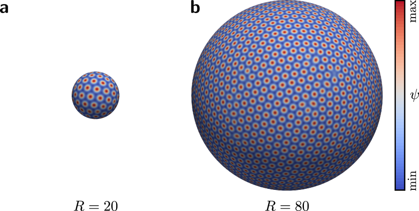
Figure 1: (Color online) Late-time density field $\psi(\mathbf{r},t)$ on spheres with radii (a) $R=20$ and (b) $R=80$, relaxed from a noisy initial density to a crystalline state containing defects for $v_{0}=0.31$.

To analyze the emerging patterns of $\psi$ and $\mathbf{p}$, we introduce some appropriate quantities.

For characterizing the density field, we identify the positions $\mathbf{r}_{i}(t)$ with $i\in\{1,\dotsc,n_{p}(t)\}$ of the local density maxima (“particle positions”), where $n_{p}(t)$ is their total number in the considered density field at time $t$. The set $\{\mathbf{r}_{i}(t)\}$ of the particle positions at time $t$ is defined as

$$\Big{\{}\mathbf{r}\,:\,\psi(\mathbf{r},t)=\max\{\psi(\mathbf{r}^{\prime},t)\,:\,\mathbf{r}^{\prime}\in\mathcal{U}(\mathbf{r})\}\Big{\}}$$ (26)

with $\mathcal{U}(\mathbf{r})=\mathcal{B}(\frac{d}{2},\mathbf{r})\cap{\mathcal{S}}$ being a neighborhood around $\mathbf{r}$ on the sphere ${\mathcal{S}}$, where $\mathcal{B}(\frac{d}{2},\mathbf{r})$ is an open ball of radius $d/2$ centered at $\mathbf{r}$ and $d=4\pi/\sqrt{3}$ is the center-to-center distance of neighboring particles in a flat hexagonal lattice with lattice constant $2\pi$. Since the positions $\mathbf{r}_{i}(t)$ can be time-dependent, we calculate also their velocities

$$\mathbf{v}_{i}(t)=\frac{1}{\tau}\big{(}\mathbf{r}_{i}(t)-\mathbf{r}_{i}(t-\tau)\big{)}\,.$$ (27)

Averaging the velocities $\mathbf{v}_{i}(t)$ locally over an appropriate time interval, which is $3000\leq t\leq 4000$ in this work, and spatial smoothing yields a continuous local velocity field $\mathbf{v}_{l}(\mathbf{r})$ that gives insights into the particle motion at late times. The mean particle speed ${v_{m}}$ in the crystalline state is obtained as

$${v_{m}}=\frac{1}{t_{\mathrm{end}}-t_{c}}\int^{t_{\mathrm{end}}}_{t_{c}}\!\!\frac{1}{n_{p}(t)}\sum^{n_{p}(t)}_{i=1}\lVert\mathbf{v}_{i}(t)\rVert\,\mathrm{d}t\,,$$ (28)

where $t_{c}$, which we chose as $t_{c}=1000$, is a sufficiently large time after which the crystalline state has formed.

To characterize the polarization field, we assign a net polarization to each density peak. For the $i$th particle, being at position $\mathbf{r}_{i}(t)$, the net polarization $\mathbf{p}_{i}(t)$ is calculated as

$$\mathbf{p}_{i}(t) =\frac{\tilde{\mathbf{p}}_{i}(t)}{\lVert\tilde{\mathbf{p}}_{i}(t)\rVert}\,,$$ (29)

$$\tilde{\mathbf{p}}_{i}(t) =\int_{\mathcal{U}(\mathbf{r}_{i}(t))}\!\!\!\!\!\!\!\!\!\!\!\!\psi^{+}(\mathbf{r},t)\,\pi_{{\mathrm{T}_{i}{{\mathcal{S}}}}}(t)\mathbf{p}(\mathbf{r},t)\,\mathrm{d}^{2}r$$ (30)

with the shifted density field $\psi^{+}(\mathbf{r},t)=\psi(\mathbf{r},t)-\min_{\mathbf{r}}(\psi(\mathbf{r},t))$, where $\min_{\mathbf{r}}(\psi(\mathbf{r},t))$ is the minimal value of $\psi$ at time $t$, and the projection $\pi_{{\mathrm{T}_{i}{{\mathcal{S}}}}}(t)$ that maps onto the tangent plane ${\mathrm{T}_{\mathbf{r}_{i}(t)}{{\mathcal{S}}}}$. We also define a coarse-grained polar order parameter

$$\mathfrak{p}_{i}(t)=\frac{1}{\mathrm{bar}{w}_{i}(t)}\sum_{\begin{subarray}{c}j\in\mathcal{J}_{t}(\mathbf{r}_{i}(t))\\ j\neq i\end{subarray}}\!\!\!w_{ij}(t)\,\mathbf{p}_{i}(t)\mathchoice{\mathbin{\vbox{\hbox{\scalebox{0.5}{$\displaystyle\bullet$}}}}}{\mathbin{\vbox{\hbox{\scalebox{0.5}{$\textstyle\bullet$}}}}}{\mathbin{\vbox{\hbox{\scalebox{0.5}{$\scriptstyle\bullet$}}}}}{\mathbin{\vbox{\hbox{\scalebox{0.5}{$\scriptscriptstyle\bullet$}}}}}\mathbf{p}_{j}(t)\,,$$ (31)

which measures the parallelity of the net polarization $\mathbf{p}_{i}(t)$ of the $i$th particle with respect to the net polarizations of the neighboring particles. In Eq. (31), $\mathcal{J}_{t}(\mathbf{r})=\{j\,:\,\lVert\mathbf{r}_{j}(t)-\mathbf{r}\rVert<r_{\mathrm{cut}}\}$ is the index set of the particles with a distance smaller than the cutoff radius $r_{\mathrm{cut}}=2.5d$ from $\mathbf{r}$ at time $t$. The weights $w_{ij}(t)$ are chosen as the inverse distance of the $i$th and $j$th particle at time $t$, i.e., $w_{ij}(t)=1/\lVert\mathbf{r}_{j}(t)-\mathbf{r}_{i}(t)\rVert$, and $\mathrm{bar}{w}_{i}(t)$ is the normalization factor

$$\mathrm{bar}{w}_{i}(t)=\sum_{\begin{subarray}{c}j\in\mathcal{J}_{t}(\mathbf{r}_{i}(t))\\ j\neq i\end{subarray}}\!\!\!w_{ij}(t)\,.$$ (32)

By spatially smoothing the discrete polar order parameters $\mathfrak{p}_{i}(t)$ with $i\in\{1,\dotsc,n_{p}(t)\}$, a continuous local polar order parameter $\mathfrak{p}(\mathbf{r},t)$ is obtained. In addition, we introduce the global polar order parameter

$$\mathcal{P}(t)=\frac{1}{n_{p}(t)}\sum^{n_{p}(t)}_{i=1}\mathfrak{p}_{i}(t)\,,$$ (33)

which is a measure for the local parallelity of the particles’ net polarizations averaged over the full sphere ${\mathcal{S}}$, and the global net polarization vector

$$\mathbf{P}(t)=\sum^{n_{p}(t)}_{i=1}\mathbf{p}_{i}(t)\,,$$ (34)

which describes the global net polarization of the active crystal.

IV Results

When calculating the time evolution of $\psi$ and $\mathbf{p}$ for small $v_{0}$, a crystalline structure builds up (see Fig. 1). The polarization field $\mathbf{p}$ then evolves to nearly the negative gradient direction of $\psi$ forming asters at the density maxima.

At a certain threshold value $v_{\mathrm{th}}$ of the activity $v_{0}$, the aster-defect positions of $\mathbf{p}$ start to depart more and more from the density maxima at $\mathbf{r}_{i}$ (see Fig. 2a),

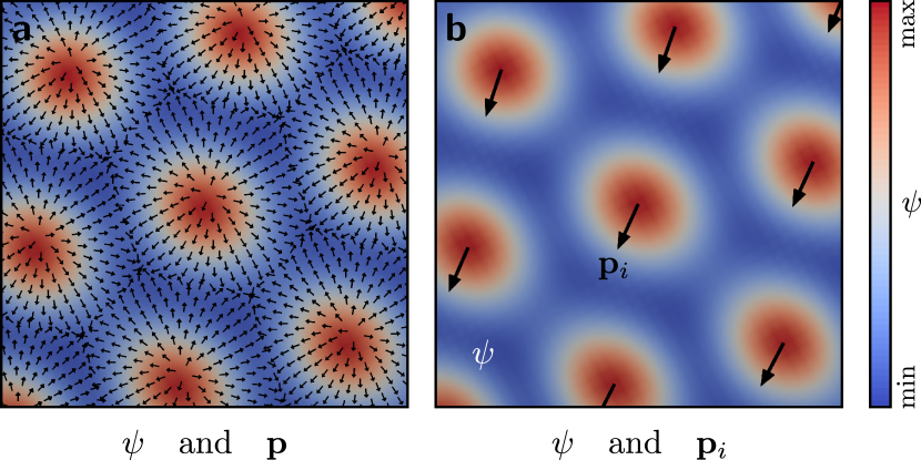
Figure 2: (Color online) Detailed view on the density field $\psi(\mathbf{r},t)$ (background color) from Fig. 1b as well as the associated (a) local polarization $\mathbf{p}(\mathbf{r},t)$ (arrows) and (b) normalized net polarizations $\mathbf{p}_{i}(t)$ (arrows at positions $\mathbf{r}_{i}$). The crystal moves in the direction of the latter arrows.

leading to nonvanishing net polarizations $\mathbf{p}_{i}$ (see Fig. 2b) and to an advection of the density field. This means that below this threshold the crystal is static, whereas above the threshold the particles in the crystal move in directions that align with the particles’ net polarizations. A similar behavior has been found in the case of a flat periodic domain in Refs. Menzel and Löwen (2013); Menzel et al. (2014); Alaimo et al. (2016). For the sphere radii $R$ considered in this work, the activity threshold $v_{\mathrm{th}}$ of the resting to motion transition is $v_{\mathrm{th}}\approx 0.3$, which is smaller than the threshold given in Ref. Menzel et al. (2014) for a flat system. Both the value for $v_{\mathrm{th}}$ observed in our simulations as well as its apparent independence from $R$ are in very good agreement with results obtained by a linear stability analysis of Eqs. (11) and (12) (see Appendix A). This stability analysis shows that $v_{\mathrm{th}}$ has in fact a nonvanishing but only weak dependence on $R$. The values of $v_{\mathrm{th}}$ vary between a minimum $v_{\mathrm{th,min}}\approx 0.28$ and slightly larger values, where the deviations from $v_{\mathrm{th,min}}$ decrease with growing $R$. For the radii $R=20$ and $R=80$ considered in our simulations, the activity threshold is $v_{\mathrm{th}}\approx 0.31$ and $v_{\mathrm{th}}\approx 0.29$, respectively, and it asymptotically gets constant for $R\to\infty$.

For activities not too far above the threshold value, the motion of the individual particles leads to a global motion pattern with a vortex-vortex configuration as shown in Fig. 3.

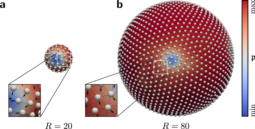
Figure 3: (Color online) Maxima (visualized as spherical particles) of the density field $\psi$ from Fig. 1 as well as the associated normalized net polarizations $\mathbf{p}_{i}$ (arrows, visible in the insets) and local polar order parameter $\mathfrak{p}$ (coloring of the sphere). The crystal has two opposing minima of $\mathfrak{p}$ and rotates about an axis through these minima.

In this configuration, the net polarizations $\mathbf{p}_{i}$ form two vortices at oppositely located poles on the sphere, resulting in a self-spinning motion of the crystal about an axis through these poles. Most of the particles in such a self-spinning crystal show a strong parallel local alignment of their net polarizations. The local polar order parameter $\mathfrak{p}(\mathbf{r},t)$ of a vortex-vortex crystal has minima at the two poles and it is maximal at the equator.

Figure 4 shows the time-averaged local particle velocity $\mathbf{v}_{l}(\mathbf{r})$ for three values of the activity parameter $v_{0}$.

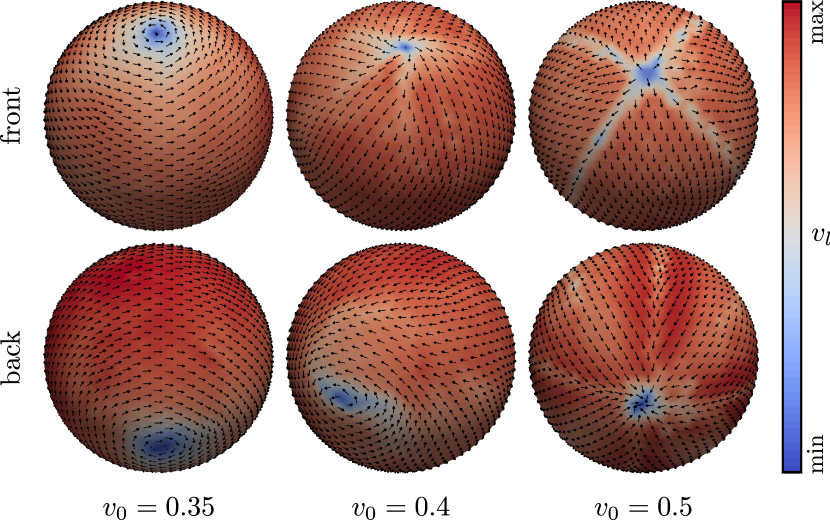
Figure 4: (Color online) Individual particle velocities $\mathbf{v}_{i}$ on a sphere with radius $R=80$ averaged over the time interval $3000\leq t\leq 4000$. The coloring of a sphere shows the time-averaged local particle speed $v_{l}(\mathbf{r})=\lVert\mathbf{v}_{l}(\mathbf{r})\rVert$ and the arrows show the time-averaged local direction of particle motion $\mathbf{v}_{l}(\mathbf{r})/v_{l}(\mathbf{r})$.

With increasing $v_{0}$ a transition from a vortex-vortex crystal (left column) to a source-sink crystal (right column) can be seen. This transition is smooth, with combinations of vortex and source or sink defects as intermediate states (middle column), and leads to a change in the qualitative behavior of the system. While the vortex-vortex crystal seems natural and can be observed directly also by classical particle simulations Sknepnek and Henkes (2015); Janssen et al. (2017), the source-sink crystal, though natural for vector fields Bowick and Giomi (2009); Sknepnek and Henkes (2015), must be interpreted in the sense that at one pole the system crystallizes, whereas at the other pole it melts. The form of Eq. (11) guarantees mass conservation, but not particle number conservation, which would be expected in a classical discrete particle model.

Classification of the observed late-time structures for different $v_{0}$ and $R$ into static, vortex-vortex, and source-sink patterns leads to the state diagram in Fig. 5.

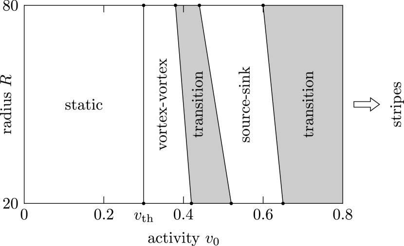
Figure 5: State diagram for different activities $v_{0}$ and sphere radii $R$ including static, vortex-vortex, and source-sink patterns as well as two broad transition regions. For activities much larger than $v_{0}=0.8$, a stripe state is found.

Except for the static to vortex-vortex transition, there are broad transition areas between neighboring states. In the transition area between the vortex-vortex and source-sink states, combinations of vortex and source or sink defects are found. When increasing the activity above $v_{0}=0.8$, a slow transition to a stripe (or lamellar) state is observed. This state is found also in the case of a plain system Menzel and Löwen (2013) and for other values of the model parameter ${\varepsilon}$ Achim et al. (2011); Stoop et al. (2015). For a rather high activity, we found traveling stripes. A more detailed study of this state is, however, beyond the scope of this work.

The dependency of the particles’ velocities on the activity parameter $v_{0}$ can be studied on the basis of the mean particle speed ${v_{m}}$. In Fig. 6, it is compared to the activity parameter.

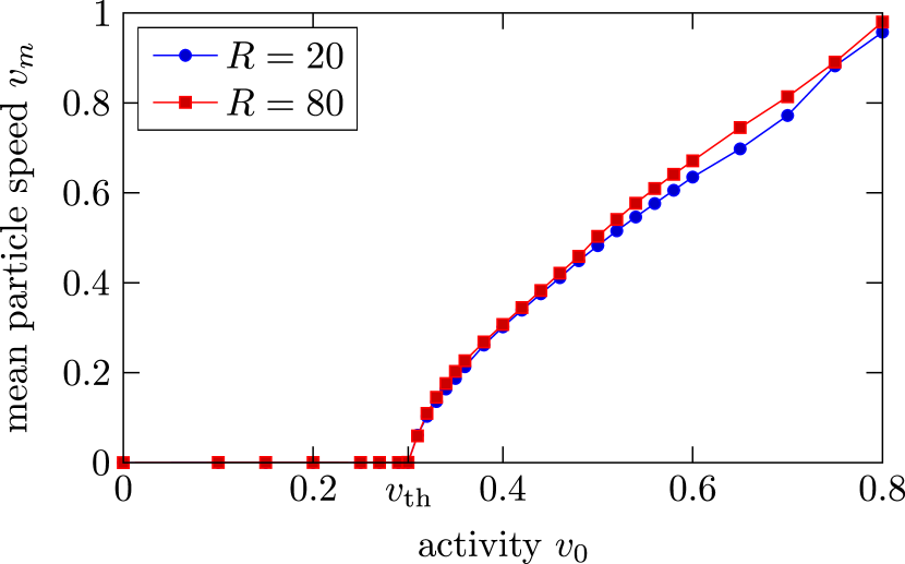
Figure 6: (Color online) Mean particle speed ${v_{m}}$ as a function of activity $v_{0}$ for spheres with radii $R=20$ and $R=80$. For both radii, the activity threshold, where the particles start to move, is $v_{\mathrm{th}}\approx 0.3$. The data are averaged over $50$ simulations.

Interestingly, the function ${v_{m}}(v_{0})$ seems to be independent of the sphere radius $R$. The observed behavior is qualitatively the same as in Refs. Menzel et al. (2014); Alaimo et al. (2016) for the flat periodic case. However, the absolute value for $v_{\text{th}}$ and the slope for ${v_{m}}(v_{0})$ differ.

The net polarizations $\mathbf{p}_{i}$ build a vector field with global polar order $\mathcal{P}$. In Fig. 7, the polar order parameter $\mathcal{P}(t)$ is visualized over a large simulation time interval for two radii $R$ of the sphere and two activity parameters $v_{0}$.

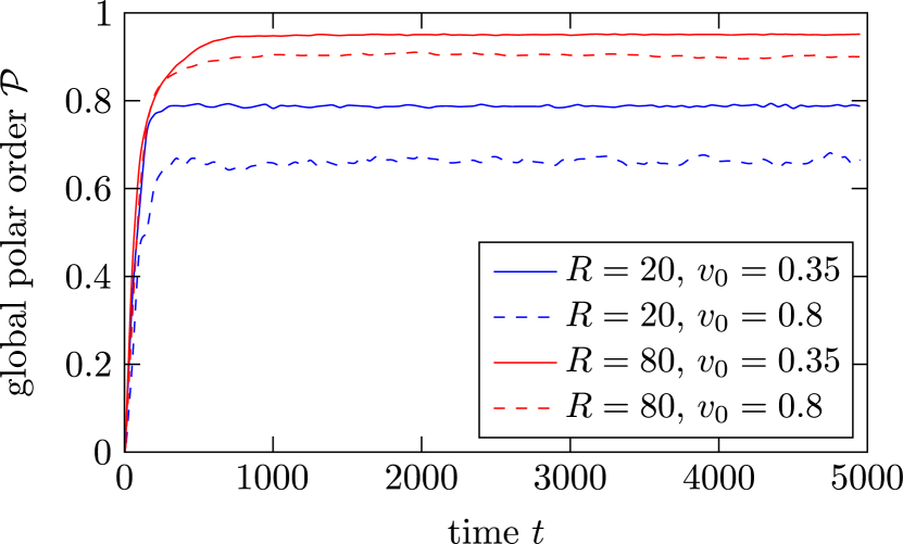
Figure 7: (Color online) Global polar order parameter $\mathcal{P}$ as a function of time $t$ for sphere radii $R=20$ and $R=80$ and activities $v_{0}=0.35$ and $v_{0}=0.8$. The data are averaged over $50$ simulations.

After an initial relaxation at $0\leq t\lesssim 1000$, the global polar order has reached its maximum and stays constant. While for $R=80$ nearly the value $\mathcal{P}=1$ is reached, a smaller sphere results in a smaller maximal global polar order. This can be explained by the larger geometrical constraints on a sphere with smaller surface area. Also a larger $v_{0}$ leads to a smaller maximal polar order, since for larger $v_{0}$ the particles are more dynamic, which hampers a parallel alignment of the net polarizations.

The different states go along also with different values of the time-averaged global net polarization $P=\lVert\mathbf{P}\rVert$ (see Fig. 8).

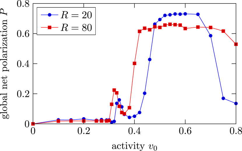
Figure 8: (Color online) Global net polarization $P=\lVert\mathbf{P}\rVert$ averaged over the time interval $1000\leq t\leq 5000$ as a function of activity $v_{0}$ for spheres with radii $R=20$ and $R=80$. The data are averaged over $50$ simulations.

In the static crystal at small $v_{0}$, the net polarizations $\mathbf{p}_{i}$ and thus the global net polarization $P$ vanish. At $v_{0}\approx 0.3$, where nonvanishing net polarizations are established and the density maxima start to move, $P$ suddenly grows; at $v_{0}\approx 0.35$ the global net polarization reaches its next minimum, which is associated with the vortex-vortex crystal; at $v_{0}\approx 0.4$ the global net polarization increases steeply until it reaches its maximum in the source-sink state. The increase of $P$ from the vortex-vortex state to the source-sink state can also be expected from the arrow fields shown in Fig. 4. For large activities $v_{0}>0.6$ the source-sink crystal gets disturbed and $P$ decreases again.

We now focus on the occurrence of translational defects (i.e., dislocations) in the crystalline states, which result from the topological constraints Bausch et al. (2003). Examples for such defects are already visible in Fig. 1. Translational defects in the crystal structure can be identified by the coordination number $\zeta_{i}$, which is equal to the number of nearest neighbors of a cell around the node $\mathbf{r}_{i}$ in a spherical Voronoi diagram with the particle positions $\{\mathbf{r}_{j}\}$ as nodes. In a defect-free hexagonal crystal one has $\zeta_{i}=6$ for all $i\in\{1,\dotsc,n_{p}\}$, but on a sphere a classical theorem of Euler states that

$$\sum_{\zeta}(6-\zeta)\mathfrak{N}_{\zeta}=6\chi({\mathcal{S}})=12\,,$$ (35)

where $\mathfrak{N}_{\zeta}$ is the number of nodes with coordination number $\zeta$ and $\chi({\mathcal{S}})=2$ is the Euler characteristic of the sphere. Typically, there are no fourfold or lower-order defects in such a crystal. Then the number of fivefold defects is at least $12$ and increases with the number and order of sevenfold and higher-order defects. Counting the total number of defects, i.e., the number of index values $i$ where $\zeta_{i}\neq 6$, shows that in our simulations between 10 and 20 percent of the particles in the static crystal ($v_{0}<0.3$) have more or less than $6$ neighbors (see Fig. 9).

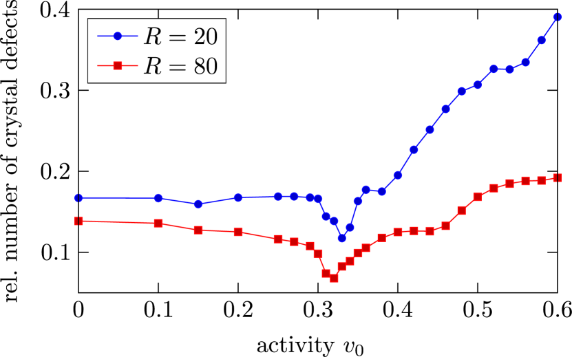
Figure 9: (Color online) Number of defects in the crystalline structure relative to the overall number of particles as a function of activity $v_{0}$ for spheres with radii $R=20$ and $R=80$. The data are averaged over the time interval $1000\leq t\leq 5000$ and over $50$ simulations.

When the activity forces the crystal to move and the vortex-vortex state emerges ($v_{0}\approx 0.3$), the particles are able to improve their spatial arrangement and the number of defects goes down. For larger activities the number of defects increases steeply and it becomes maximal in the source-sink state. This is consistent with the plots in Figs. 1 and 4, which also indicate that the source-sink crystal contains more defects than the other crystalline states.

To study the defects in more detail, we now look at chains formed by defects of different coordination numbers (e.g., pairs of five-fold and seven-fold defects). In Fig. 10, only the particles with coordination numbers $\zeta_{i}\neq 6$ are shown.

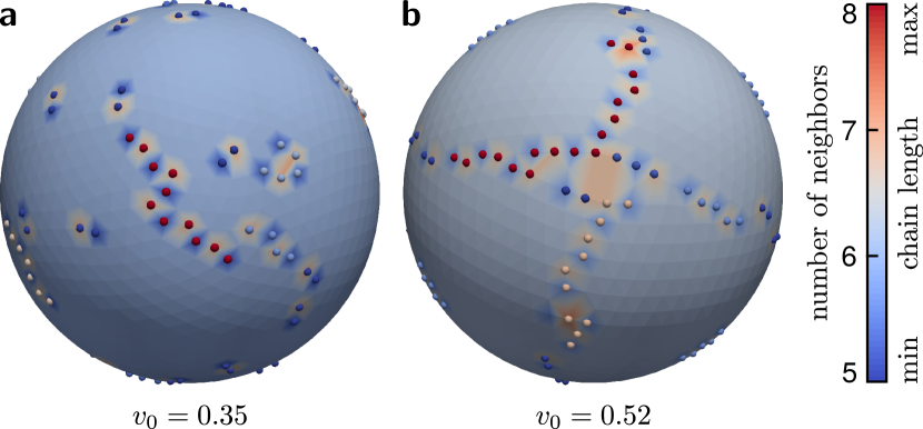
Figure 10: (Color online) Chains of defects on a sphere with radius $R=80$ at late times for activities (a) $v_{0}=0.35$ and (b) $v_{0}=0.52$. Defects are visualized as small spheres, whose colors indicate the length of the corresponding defect chain. The coloring of the large sphere near a defect depicts the number of maxima of the density field $\psi$ neighboring the defect, where dark blue means 5 neighbors and orange denotes 7 neighbors. Light blue regions of the large sphere are free of defects.

There are separated pairs of defects, but also long chains of defects. This is similar to the passive case ($v_{0}=0$) for various geometries Bausch et al. (2003); Irvine et al. (2010); Bendito et al. (2013); Schmid and Voigt (2014), but here the chains of defects are dynamic. Due to the activity of the particles, the defect chains permanently emerge, move, change size, and vanish. The numbers of defects located in these chains are statistically analyzed in Fig. 11 for various activities $v_{0}$.

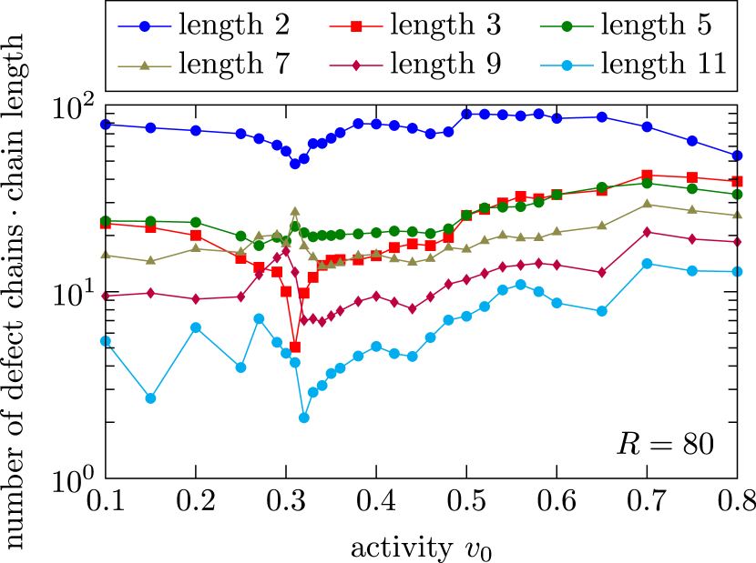
Figure 11: (Color online) The number of defect chains of a particular length on a sphere with radius $R=80$ multiplied by the chain length, i.e., the total number of defects that are part of the defect chains of this length, as a function of activity $v_{0}$ for six different chain lengths. In the activity range $0.3\lesssim v_{0}\lesssim 0.32$, the numbers of chains with lengths $5$, $7$, and $9$ increase, whereas the numbers of chains with the other lengths decrease. The data are averaged over the time interval $1000\leq t\leq 5000$ and over $50$ simulations.

Already for small activities there are defect chains of all considered lengths present. Short chains consisting of only two defects are most frequent, whereas with growing length the chains become increasingly rare. This is an overall trend and true for most activities. An exception constitute activities near the threshold value $v_{\mathrm{th}}\approx 0.3$, where the overall number of defects in the system is minimal. For such activities, the number of defect chains as a function of the activity $v_{0}$ has an extremum for all chain lengths. Especially very short chains with lengths $2$ and $3$ are less frequent for $v_{0}\approx v_{\mathrm{th}}$ than for smaller or larger values of $v_{0}$. In contrast, the numbers of longer chains with lengths $5$, $7$, and $9$ have a maximum near the threshold activity $v_{\mathrm{th}}$. This means that the vortex-vortex state favors the formation of these longer defect chains. For larger activities, where the overall number of defects grows with $v_{0}$, the number of defect pairs first increases but later decreases again, whereas the chains consisting of more than two defects increase in number.

V Conclusions and outlook

Using a new active phase-field-crystal-type model we have studied crystals of self-propelled colloidal particles on a sphere. These “active crystals” have a hexagonal local density pattern and – due to the topological constraints prescribed by the sphere – always some defects. Three types of crystals are observed: a static crystal, a vortex-vortex crystal, and a source-sink crystal. When relaxing the particle density field from a random initial density distribution, the number of defects at low activity is $10$-$20$ percent of the total particle number and can be minimized by choosing an activity that corresponds to the vortex-vortex state. It should be possible to confirm the observed crystalline states and the results related to their defects by particle-resolved simulations and experiments.

With the numerical tools for vector-valued surface partial differential equations developed in Refs. Witkowski et al. (2015); Nestler et al. (2018); Reuther and Voigt (2018), the problem can even be considered on nonspherical geometries. It would also be interesting to use PFC models to study nonspherical self-propelled particles and their active liquid-crystalline states Sanchez et al. (2012); Wensink et al. (2012) on a sphere Janssen et al. (2017) and other manifolds Nestler et al. (2017); Sitta et al. (2018). Appropriate PFC models could be obtained by extending the existing PFC models for liquid crystals Wittkowski et al. (2010, 2011a, 2011b); Achim et al. (2011); Praetorius et al. (2013) towards active particles and curved manifolds.

Appendix A Linear stability analysis

In this appendix, we carry out a linear stability analysis to get more insights into the properties of the PFC model given by Eqs. (11) and (12). For this stability analysis, we consider a homogeneous stationary state with local density $\mathrm{bar}{\psi}$ and vanishing local polarization. When this state is slightly perturbed, $\psi(\mathbf{r},t)$ and $\mathbf{p}(\mathbf{r},t)$ can be written as

$$\psi(\mathbf{r},t) =\mathrm{bar}{\psi}+\delta\psi(\mathbf{r},t)\,,$$ (36)

$$\mathbf{p}(\mathbf{r},t) =\delta\mathbf{p}(\mathbf{r},t)\,,$$ (37)

where $\delta\psi(\mathbf{r},t)$ and $\delta\mathbf{p}(\mathbf{r},t)$ are the small perturbations of the density and polarization fields, respectively. Inserting Eqs. (36) and (37) into Eqs. (11) and (12) and subsequent linearization with respect to the perturbations results in the equations

$$\begin{split}\partial_{t}\delta\psi&=\boldsymbol{\triangle}_{{\mathcal{S}}}\big{(}\big{(}3\mathrm{bar}{\psi}^{2}+{\varepsilon}+(1+\boldsymbol{\triangle}_{{\mathcal{S}}})^{2}\big{)}\delta\psi\big{)}\\ &\quad\>\!\>\!-v_{0}\,{\operatorname{div}_{{\mathcal{S}}}}\delta\mathbf{p}\,,\end{split}$$ (38)

$$\begin{split}\partial_{t}\delta\mathbf{p}&=-C_{1}(\boldsymbol{\triangle}_{\mathrm{dR}}+D_{r})\delta\mathbf{p}-v_{0}\,{\operatorname{grad}_{{\mathcal{S}}}}\delta\psi\end{split}$$ (39)

that describe the initial time evolution of the perturbations. Next, we expand the perturbations as

$$\delta\psi(\mathbf{r},t) =\!\!\!\sum_{(l,m)\in\,\mathcal{I}_{\infty}}\!\!\!\hat{\delta\psi}_{lm}(t)Y_{l}^{m}(\mathbf{r})\,,$$ (40)

$$\delta\mathbf{p}(\mathbf{r},t) =\sum_{i=1}^{2}\sum_{(l,m)\in\,\mathcal{I}_{\infty}}\!\!\!\hat{\delta p}_{lm}^{(i)}(t)\mathbf{y}_{lm}^{(i)}(\mathbf{r})\,.$$ (41)

This leads to ordinary differential equations for the time-evolution of the expansion coefficients $\hat{\delta\psi}_{lm}(t)$ and $\hat{\delta p}_{lm}^{(i)}(t)$. When defining the perturbation mode vector $\delta\boldsymbol{\hat{\Xi}}=(\hat{\delta\psi}_{lm},\hat{\delta p}_{lm}^{(1)},\hat{\delta p}_{lm}^{(2)})^{\mathrm{T}}$, these time-evolution equations can be written as

$$\partial_{t}\delta\boldsymbol{\hat{\Xi}}=-\boldsymbol{\mathrm{M}}\,\delta\boldsymbol{\hat{\Xi}}$$ (42)

with the matrix $\boldsymbol{\mathrm{M}}=(M_{ij})_{i,j=1,2,3}$, whose elements $M_{ij}$ are given by

$$M_{11} =\frac{l(l+1)}{R^{2}}\Big{(}3\mathrm{bar}{\psi}^{2}+{\varepsilon}+\Big{(}1-\frac{l(l+1)}{R^{2}}\Big{)}^{2}\Big{)}\,,$$ (43)

$$M_{12} =-v_{0}\frac{l(l+1)}{R}\,,$$ (44)

$$M_{21} =\frac{v_{0}}{R}\,,$$ (45)

$$M_{22} =M_{33}=C_{1}\Big{(}\frac{l(l+1)}{R^{2}}+D_{r}\Big{)}\,,$$ (46)

$$M_{13} =M_{31}=M_{23}=M_{32}=0\,.$$ (47)

The three eigenvalues of this matrix are given by $\Lambda_{1}=M_{22}$ and $\Lambda_{2,3}=(M_{11}+M_{22}\pm\sqrt{D})/2$ with the real-valued $D=(M_{11}-M_{22})^{2}+4M_{12}M_{21}$.

We know that the homogeneous state of the model is stable when the real parts of all eigenvalues are positive and that it is unstable when at least one eigenvalue has a negative real part. Otherwise the linear stability analysis does not permit an assessment of the stability of the homogeneous state. Taking into account that the signs of $M_{22}$ and $C_{1}$ are equal, since always $R>0$, $D_{r}>0$, and $l\geq 0$, we find the following stability criteria: The homogeneous state is

• stable if $C_{1}>0\,\wedge\,\forall l\,:\,M_{11}+M_{22}-\Re(\sqrt{D})>0$ and

• unstable if $C_{1}<0\,\vee\,\exists l\,:\,M_{11}+M_{22}-\Re(\sqrt{D})<0$.

Here, $\Re(\sqrt{D})$ denotes the real part of $\sqrt{D}$. In the case of an unstable homogeneous state, small perturbations grow with time and $\psi(\mathbf{r},t)$ and $\mathbf{p}(\mathbf{r},t)$ become strongly inhomogeneous as in the crystalline states described in Sec. IV. Regarding the unstable case, we can distinguish two situations: When $D\geq 0$, the amplitudes of the inhomogeneities grow with time, but their positions are static; in contrast, for $D<0$, traveling inhomogeneities emerge, since the eigenvalues $\Lambda_{2}$ and $\Lambda_{3}$ are then complex conjugates of each other (see Ref. Wittkowski et al. (2017) for details). This finding is highly interesting, since it is analogous to the observation of static and traveling crystals in the simulations.

To consider this finding in more detail, we evaluated the aforementioned stability criteria for parameter values that correspond to our simulations. Remarkably, in these stability criteria the (vector) spherical harmonics degree $l$ and the sphere radius $R$ occur always together as the degree parameter $l(l+1)/R^{2}$. Therefore, we varied $l(l+1)/R^{2}$ and $v_{0}$ and chose the other parameters as in Tab. 1. This yields the stability diagram presented in Fig. 12.

Figure 12: (Color online) Stability diagram showing for various sphere radii $R$ and activities $v_{0}$ the degrees $l$ of (vector) spherical harmonic perturbations to which a homogeneous state of the PFC model given by Eqs. (11) and (12) with local density $\mathrm{bar}{\psi}$ and vanishing local polarization is stable (blue) or unstable (green or red). The emergence of inhomogeneities leads to the formation of pronounced patterns, where static inhomogeneities (green) correspond to the static crystal and traveling inhomogeneities (red) to the dynamic patterns shown in Fig. 5.

It shows that for all considered activities $v_{0}$, the homogeneous state of the PFC model given by Eqs. (11) and (12) is unstable to (vector) spherical harmonic perturbations whose degree $l$ is within a certain range of values. This is in accordance with the fact that we observed the formation of an inhomogeneous state for all parameter combinations considered in this work. The band of degrees $l$ associated with unstable modes depends on $R$ in such a way that $l(l+1)/R^{2}$ is constant for corresponding modes in systems with different $R$. Hence, the values of $l$ associated with unstable modes increase with $R$. This is reasonable, since the emerging inhomogeneities are subject to the fixed lattice constant of $2\pi$ preferred by the model. Furthermore, the stability diagram shows that the emerging inhomogeneities are static for small $v_{0}$ and traveling for large $v_{0}$. This is in line with the observation of the activity threshold $v_{\mathrm{th}}$ in Fig. 6. In the stability diagram in Fig. 12, the activity threshold is the smallest value of $v_{0}$ for which a positive integer $l$ associated with an unstable mode exists. Therefore, by simultaneously solving the equations $M_{11}+M_{22}=0$ and $D=0$ with respect to $l(l+1)/R^{2}$ and $v_{0}$ and by choosing the solution with the smallest positive $v_{0}$, we calculated the coordinates $(l(l+1)/R^{2},v_{0})=(\alpha_{\mathrm{th,min}},v_{\mathrm{th,min}})\approx(0.63,0.28)$ of the point in the left bottom corner of the red area in the stability diagram. The activity value $v_{\mathrm{th,min}}\approx 0.28$ is the threshold activity $v_{\mathrm{th}}$ for all $R$ for which the equation $l(l+1)/R^{2}=\alpha_{\mathrm{th,min}}$ has a positive integer solution for $l$. For all other not too small $R$, the value of $v_{\mathrm{th}}$ is slightly larger, since it corresponds to the lowest point on the border between the green and red areas in Fig. 12 for which $l$ is integer. An exception constitute only too small radii $R\lesssim 2$, for which the equation has no positive integer solution. This means that for $R\gtrsim 2$, the activity threshold $v_{\mathrm{th}}$ has only a weak dependence on $R$. Its values vary between $v_{\mathrm{th,min}}$ and slightly larger values, where the deviations from $v_{\mathrm{th,min}}$ decrease for growing $R$ and asymptotically vanish for $R\to\infty$. For the radii $R=20$ and $R=80$ used in our simulations, the activity threshold is $v_{\mathrm{th}}\approx 0.31$ and $v_{\mathrm{th}}\approx 0.29$, respectively. This is in very good agreement with the threshold value $v_{\mathrm{th}}\approx 0.3$ in Fig. 6 and its apparent independence of $R$.

References

- Nelson (2002) D. R. Nelson, Defects and Geometry in Condensed Matter Physics (Cambridge University Press, New York, 2002).
- Bowick and Giomi (2009) M. J. Bowick and L. Giomi, Adv. Phys. 58, 449 (2009).
- Smale (1998) S. Smale, Math. Intell. 20, 7 (1998).
- Backofen et al. (2011) R. Backofen, M. Gräf, D. Potts, S. Praetorius, A. Voigt, and T. Witkowski, Multiscale Model. Sim. 9, 314 (2011).
- Agricola and Friedrich (2002) I. Agricola and T. Friedrich, Global Analysis: Differential Forms in Analysis, Geometry, and Physics, 1st ed., Graduate Studies in Mathematics, Vol. 52 (American Mathematical Society, Providence, 2002).
- Ramaswamy (2010) S. Ramaswamy, Annu. Rev. Condens. Mat. Phys. 1, 323 (2010).
- Romanczuk et al. (2012) P. Romanczuk, M. Bär, W. Ebeling, B. Lindner, and L. Schimansky-Geier, Eur. Phys. J. Spec. Top. 202, 1 (2012).
- Elgeti et al. (2015) J. Elgeti, R. G. Winkler, and G. Gompper, Rep. Prog. Phys. 78, 056601 (2015).
- Menzel (2015) A. M. Menzel, Phys. Rep. 554, 1 (2015).
- Bechinger et al. (2016) C. Bechinger, R. Di Leonardo, H. Löwen, C. Reichhardt, G. Volpe, and G. Volpe, Rev. Mod. Phys. 88, 045006 (2016).
- Bialké et al. (2012) J. Bialké, T. Speck, and H. Löwen, Phys. Rev. Lett. 108, 168301 (2012).
- Redner et al. (2013) G. S. Redner, M. F. Hagan, and A. Baskaran, Phys. Rev. Lett. 110, 055701 (2013).
- Menzel and Löwen (2013) A. M. Menzel and H. Löwen, Phys. Rev. Lett. 110, 055702 (2013).
- Ferrante et al. (2013) E. Ferrante, A. E. Turgut, M. Dorigo, and C. Huepe, New J. Phys. 15, 095011 (2013).
- Menzel et al. (2014) A. M. Menzel, T. Ohta, and H. Löwen, Phys. Rev. E 89, 022301 (2014).
- Briand and Dauchot (2016) G. Briand and O. Dauchot, Phys. Rev. Lett. 117, 098004 (2016).
- Drescher et al. (2010) K. Drescher, R. E. Goldstein, and I. Tuval, Proc. Nat. Acad. Sci. U.S.A. 107, 11171 (2010).
- Juarez and Stocker (2014) G. Juarez and R. Stocker, in APS Division of Fluid Dynamics Meeting Abstracts (2014).
- Vladescu et al. (2014) I. D. Vladescu, E. J. Marsden, J. Schwarz-Linek, V. A. Martinez, J. Arlt, A. N. Morozov, D. Marenduzzo, M. E. Cates, and W. C. K. Poon, Phys. Rev. Lett. 113, 268101 (2014).
- Keber et al. (2014) F. C. Keber, E. Loiseau, T. Sanchez, S. J. DeCamp, L. Giomi, M. J. Bowick, M. C. Marchetti, Z. Dogic, and A. R. Bausch, Science 345, 1135 (2014).
- Großmann et al. (2015) R. Großmann, F. Peruani, and M. Bär, Eur. Phys. J. Spec. Top. 224, 1377 (2015).
- Li (2015) W. Li, Sci. Rep. 5, 13603 (2015).
- Sknepnek and Henkes (2015) R. Sknepnek and S. Henkes, Phys. Rev. E 91, 022306 (2015).
- Alaimo et al. (2017) F. Alaimo, C. Köhler, and A. Voigt, Sci. Rep. 7, 5211 (2017).
- Elder et al. (2002) K. R. Elder, M. Katakowski, M. Haataja, and M. Grant, Phys. Rev. Lett. 88, 245701 (2002).
- Elder and Grant (2004) K. R. Elder and M. Grant, Phys. Rev. E 70, 051605 (2004).
- van Teeffelen et al. (2009) S. van Teeffelen, R. Backofen, A. Voigt, and H. Löwen, Phys. Rev. E 79, 051404 (2009).
- Emmerich et al. (2012) H. Emmerich, H. Löwen, R. Wittkowski, T. Gruhn, G. I. Tóth, G. Tegze, and L. Gránásy, Adv. Phys. 61, 665 (2012).
- Khoromskaia and Alexander (2017) D. Khoromskaia and G. P. Alexander, New J. Phys. 19, 103043 (2017).
- Fily et al. (2016) Y. Fily, A. Baskaran, and M. F. Hagan, preprint, arXiv:1601.00324 (2016).
- Shankar et al. (2017) S. Shankar, M. J. Bowick, and M. C. Marchetti, Phys. Rev. X 7, 031039 (2017).
- Yao (2016) Z. Yao, Soft Matter 12, 7020 (2016).
- Alaimo et al. (2016) F. Alaimo, S. Praetorius, and A. Voigt, New J. Phys. 18, 083008 (2016).
- Backofen et al. (2010) R. Backofen, A. Voigt, and T. Witkowski, Phys. Rev. E 81, 025701 (2010).
- Nestler et al. (2018) M. Nestler, I. Nitschke, S. Praetorius, and A. Voigt, J. Nonlinear Sci. 28, 147 (2018).
- Köhler et al. (2016) C. Köhler, R. Backofen, and A. Voigt, Phys. Rev. Lett. 116, 135502 (2016).
- Freeden et al. (1994) W. Freeden, T. Gervens, and M. Schreiner, Manuscr. Geodaet. 19, 80 (1994).
- Freeden and Schreiner (2009) W. Freeden and M. Schreiner, Spherical Functions of Mathematical Geosciences – A Scalar, Vectorial, and Tensorial Setup, Advances in Geophysical and Environmental Mechanics and Mathematics (Springer, Berlin, 2009).
- Hesthaven et al. (2007) J. S. Hesthaven, S. Gottlieb, and D. Gottlieb, Spectral Methods for Time-Dependent Problems (Cambridge University Press, New York, 2007).
- Schaeffer (2013) N. Schaeffer, Geochem. Geophys. 14, 751 (2013).
- Janssen et al. (2017) L. M. C. Janssen, A. Kaiser, and H. Löwen, Sci. Rep. 7, 5667 (2017).
- Achim et al. (2011) C. V. Achim, R. Wittkowski, and H. Löwen, Phys. Rev. E 83, 061712 (2011).
- Stoop et al. (2015) N. Stoop, R. Lagrange, D. Terwagne, P. M. Reis, and J. Dunkel, Nat. Mater. 14, 337 (2015).
- Bausch et al. (2003) A. R. Bausch, M. J. Bowick, A. Cacciuto, A. D. Dinsmore, M. F. Hsu, D. R. Nelson, M. G. Nikolaides, A. Travesset, and D. A. Weitz, Science 299, 1716 (2003).
- Irvine et al. (2010) W. Irvine, V. Vitteli, and P. Chaikin, Nature 468, 947 (2010).
- Bendito et al. (2013) E. Bendito, E. J. Bowick, A. Medina, and Z. Yao, Phys. Rev. E 88, 012405 (2013).
- Schmid and Voigt (2014) V. Schmid and A. Voigt, Soft Matter 10, 4694 (2014).
- Witkowski et al. (2015) T. Witkowski, S. Ling, S. Praetorius, and A. Voigt, Adv. Comput. Math. 41, 1145 (2015).
- Reuther and Voigt (2018) S. Reuther and A. Voigt, Phys. Fluids 30, 012107 (2018).
- Sanchez et al. (2012) T. Sanchez, D. T. N. Chen, S. J. DeCamp, M. Heymann, and Z. Dogic, Nature 491, 431 (2012).
- Wensink et al. (2012) H. H. Wensink, J. Dunkel, S. Heidenreich, K. Drescher, R. E. Goldstein, H. Löwen, and J. M. Yeomans, Proc. Nat. Acad. Sci. U.S.A. 109, 14308 (2012).
- Nestler et al. (2017) M. Nestler, I. Nitschke, S. Praetorius, H. Löwen, and A. Voigt, preprint, arXiv:1709.09436v1 (2017).
- Sitta et al. (2018) C. E. Sitta, F. Smallenburg, R. Wittkowski, and H. Löwen, Phys. Chem. Chem. Phys. in print (2018), DOI:10.1039/C7CP07026H.
- Wittkowski et al. (2010) R. Wittkowski, H. Löwen, and H. R. Brand, Phys. Rev. E 82, 031708 (2010).
- Wittkowski et al. (2011a) R. Wittkowski, H. Löwen, and H. R. Brand, Phys. Rev. E 83, 061706 (2011a).
- Wittkowski et al. (2011b) R. Wittkowski, H. Löwen, and H. R. Brand, Phys. Rev. E 84, 041708 (2011b).
- Praetorius et al. (2013) S. Praetorius, A. Voigt, R. Wittkowski, and H. Löwen, Phys. Rev. E 87, 052406 (2013).
- Wittkowski et al. (2017) R. Wittkowski, J. Stenhammar, and M. E. Cates, New J. Phys. 19, 105003 (2017).