Tumbling dynamics of inertial chains in extensional flow

Abstract

The dynamics of elongated inertial particles in an extensional flow is studied numerically by performing simulations of freely jointed bead-rod chains. The coil-stretch transition and the tumbling instability are characterized as a function of three parameters: The Peclet number, the Stokes number and the chain length. Numerical results show that in the limit of infinite chain length, particles are trapped in a coiled or stretched state. The coil-stretch transition is also shown to depend non-linearly on the Stokes and Peclet number. Results also reveal that tumbling occurs close to the coil-stretch transition and that the persistence time is a non-linear function of Stokes and Peclet numbers.

I Introduction

The dynamics of long, flexible and deformable particles has attracted a lot of attention in the past few years. It has notable consequences in various applications such as: The paper-making industry (where the dynamics of fibers directly impact the properties of paper, see, e.g., Lundell et al. (2011); Cui and Grace (2007)), DNA and polymer physics (where the presence of polymers in a solution can profoundly affect the rheology of the solution Shaqfeh (2005)), biological oceanography (with the central role played by plankton such as diatoms which form chain-like colonies Jumars et al. (2009); Young et al. (2012)) or atmospheric sciences (where non-spherical ice crystals impact particle-cloud interactions Pruppacher et al. (1998)). The challenges associated to such complex systems include the description of their dynamics and conformation in complex flows as well as their effect on rheological properties of fluids (see e.g. reviews Shaqfeh (2005); Lindner and Shelley (2015); Voth and Soldati (2017)). This has led to a renewed attention on the dynamics of complex-shaped objects such as solid spheroids Pumir and Wilkinson (2011); Parsa et al. (2012); Vincenzi (2013); Gustavsson et al. (2014); Gupta et al. (2014), ellipsoids Chevillard and Meneveau (2013), solid helicoids Gustavsson and Biferale (2016) as well as flexible objects such as elastic dumbbells Musacchio and Vincenzi (2011) or trumbbells Plan and Vincenzi (2016); Ali et al. (2016), flexible fibers Brouzet et al. (2014); Perkins et al. (1994, 1995); Verhille and Bartoli (2016).

In this paper, we focus on the dynamics of elongated and deformable particles. Recent experimental studies on elastic filaments have revealed a complex non-linear dynamics characterized by coil-stretch transitions (i.e. the shift from extended to folded conformations), tumbling and buckling instabilities in various simple flows (such as extensional flows Kantsler and Goldstein (2012); Hsiao et al. (2017), shear flows Harasim et al. (2013)) as well as more complex flows (such as random flows Liu and Steinberg (2010), chaotic flows Chertkov (2000), the flow past an obstacle López et al. (2015) or in a microchannel Strelnikova et al. (2017)). The ability of such elongated particles to deform under various flow conditions has also been characterized in numerous theoretical and numerical studies (see e.g. Cruz et al. (2012); Larson (2005); Lindner and Shelley (2015); Shaqfeh (2005); Underhill and Doyle (2004) and references therein). In particular, the coil-stretch transition has been reproduced using various level of descriptions for elongated particles, including fine simulations based on the slender-body theory (SBT) Lindner and Shelley (2015); Kratky and Porod (1949) or coarse-grained models such as the freely jointed bead-rod, bead-spring models or even simple dumbbells Larson (2005); Bird et al. (1987). The coil-stretch (CS) transition and tumbling statistics have been characterized recently using simple representations of elongated particles such as rigid rods/spheroids Marchioli et al. (2010); Mortensen et al. (2008), spring dumbbells Puliafito and Turitsyn (2005) or trumbbells Ali et al. (2016); Plan and Vincenzi (2016)). For instance, the phenomenon of tumbling, which is associated to elongated particles in shear flows, has been shown to occur even in stretching- dominated flow using a trumbbell model immersed in a planar extensional flow Plan and Vincenzi (2016).

Following these recent studies, the aim of the present study is to study the CS transition and tumbling instability in the case of infinitely long particles in extensional flows with stochastic noise. For that purpose, we focus on freely jointed bead-rod chains where fibers are discretized as a chain of elementary beads connected by rigid rods (also called Kramers chains Kramers (1944)). We introduce a high-order numerical method to impose the holonomic constraints in the presence of a stochastic term. A similar approach based on bead-spring chains has recently shown that fibers are trapped in either coiled or stretched states in the limit of infinite chain sizes and small-enough diffusion Beck and Shaqfeh (2007) in linear and non-linear extensional flows. It remains to be seen whether such conclusions remain valid when inertial effects are taken into account and when a bead-rod description of long particles is used. This is the scope of the present article.

For that purpose, the dynamics of inertial fibers in a flow is presented in Section II which provides details on the model used for bead-rod chains (see Section II.1) together with a theoretical analysis of the stationary states (in Section  II.2) as well as details on the numerical implementation used (see Section II.3). Then, numerical results are analyzed first for the Coil-Stretch transition in Section III and then for fiber tumbling in Section IV.

II Model and theoretical analysis

II.1 Dynamics of inertial fibers

II.1.1 Equation of motion for inertial fibers

Generic case.

We consider a suspension of inertial fibers embedded in an ambient flow and experiencing a viscous drag. Each fiber is represented as a bead-rod Kramers chain, i.e. constituted of $N+1$ beads connected by $N$ rigid bonds . Each bead labeled $i$ has a given position denoted by $\bm{X}_{i}$ and is maintained at a fixed distance $\ell_{\rm K}$ from consecutive beads in the chain (corresponding to the Kuhn length). Each bead can undergo a free angular motion relative to its neighbors while remaining at a fixed distance $\ell_{\rm K}$ from them (see Fig. 1). We have further assumed that all beads are identical with a given mass $m$.

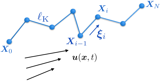
Figure 1: The flexible fiber is approximated as a bead-rod Kramers chain. The beads $\bm{X}_{i}$’s are linked together by infinitesimal rigid rods of length $\ell_{\rm K}$. The orientation of the links is given by the unitary vectors $\bm{\xi}_{i}=(\bm{X}_{i}-\bm{X}_{i-1})/\ell_{\rm K}$.

Following Newton’s second law, the individual motion of each bead reads

$$m\,\frac{{\rm d}^{2}\bm{X}_{i}}{{\rm d}t^{2}} = -\zeta\left[\frac{{\rm d}\bm{X}_{i}}{{\rm d}t}-\bm{u}(\bm{X}_{i},t)\right]+\sqrt{2k_{\rm B}T\,\zeta}\,\bm{\eta}_{i}$$ (1)

$$+\lambda_{i}\,(\bm{X}_{i}-\bm{X}_{i-1})-\lambda_{i+1}\,(\bm{X}_{i+1}-\bm{X}_{i}),$$

The first term on the right-hand side (RHS) corresponds to the Stokes drag of the beads with a prescribed velocity field $\bm{u}$ and $\zeta$ denotes the individual drag coefficient of the particles. The second term on the RHS stands for the effect of thermal fluctuations on each bead: $\bm{\eta}_{i}$ are independent isotropic white noises, with $T$ denoting the fluid absolute temperature and $k_{\rm B}$ the Boltzmann constant. The third and fourth terms on the RHS accounts for the tension (or internal forces) within a fiber: $\lambda_{i}$ is thus the tension between the $i$-th and the $(i-1)$-th beads. Unlike spring-bead models where the tension is given by a spring force (such as Hookean spring as in Rouse Jr (1953)), the tensions are here time-dependent Lagrange multipliers associated to the the holonomic constraint $|\bm{X}_{i}-\bm{X}_{i-1}|=\ell_{\rm K}$, which implies that

$$\frac{{\rm d}}{{\rm d}t}\left|\bm{X}_{i}-\bm{X}_{i-1}\right|^{2} = \frac{{\rm d}^{2}}{{\rm d}t^{2}}\left|\bm{X}_{i}-\bm{X}_{i-1}\right|^{2}=0.$$ (2)

Using Eq.(1), the tensions satisfy the system

$$0 = \left[\bm{X}_{i}-\bm{X}_{i-1}\right]\cdot\left\{\zeta\left[\bm{u}(\bm{X}_{i},t)-\bm{u}(\bm{X}_{i-1},t)\right]\right.$$ (3)

$$+\sqrt{2k_{\rm B}T\,\zeta}\,\left[\bm{\eta}_{i}-\bm{\eta}_{i-1}\right]+2\lambda_{i}\,(\bm{X}_{i}-\bm{X}_{i-1})$$

$$-\left.\lambda_{i+1}\,(\bm{X}_{i+1}-\bm{X}_{i})-\lambda_{i-1}\,(\bm{X}_{i-1}-\bm{X}_{i-2})\right\}$$

$$+\left|\frac{{\rm d}(\bm{X}_{i}-\bm{X}_{i-1})}{{\rm d}t}\right|^{2}.$$

Small fibers in an extensional flow.

In the following, we consider that the whole fiber size is below the smallest scale of variation of the fluid velocity field $\bm{u}$. In that case, the flow stretching is uniform along the chain since all beads feel the same value $\bm{\nabla}\bm{u}$ of the fluid gradient. It is then more natural to reformulate the dynamics in terms of the link unitary directions $\bm{\xi}_{i}=(\bm{X}_{i}-\bm{X}_{i-1})/\ell_{\rm K}$, that is

$$\frac{{\rm d}^{2}\bm{\xi}_{i}}{{\rm d}t^{2}} = -\frac{\zeta}{m}\left[\frac{{\rm d}\bm{\xi}_{i}}{{\rm d}t}-\bm{\xi}_{i}\cdot\bm{\nabla}\bm{u}\right]+2\lambda_{i}\,\bm{\xi}_{i}-\lambda_{i+1}\,\bm{\xi}_{i+1}$$ (4)

$$-\lambda_{i-1}\,\bm{\xi}_{i-1}+\sqrt{\frac{2k_{\rm B}T\,\zeta}{m^{2}\ell_{\rm K}^{2}}}\,(\bm{\eta}_{i}-\bm{\eta}_{i-1}),$$

The $\lambda_{i}$’s are again Lagrangian multipliers associated to the holonomic constraint (constant distance $\ell_{\rm K}$ between beads), this time reading $|\bm{\xi}_{i}|=1$.

We further assume that the fluid gradient is given by the simple case of a 2D extensional flow: The fluid is stretching in the horizontal direction $x$ while it is compressing in the vertical direction $y$ (see also Fig. 1). The velocity gradient then simplifies to:

$$\bm{\nabla}\bm{u}=\begin{pmatrix}\sigma&0\\ 0&-\sigma\end{pmatrix},$$ (5)

where $\sigma>0$ denotes the local fluid velocity shear rate.

II.1.2 Dimensionless parameters

With the assumption that $\bm{\nabla}\bm{u}$ depends on a single time scale $\tau_{\rm fluid}=\sigma^{-1}$, the problem depends upon three dimensionless parameters:

• The Stokes number, which is the ratio between the beads response time and the fluid flow timescale

  $${\rm St}=\frac{\tau_{\rm beads}}{\tau_{\rm fluid}}=\frac{\sigma\,m}{\zeta};$$ (6)

  It measures the inertia of fibers: $\rm St\ll 1$ corresponds to the case of tracers (i.e. particles following the streamlines) while $\rm St\gg 1$ designate particles that depart from the fluid streamlines.

• The Péclet number, given by the ratio between the diffusion and the advection timescales

  $${\rm Pe}=\frac{\tau_{\rm diff}}{\tau_{\rm fluid}}=\frac{\sigma\,\ell_{\rm K}^{2}\,\zeta}{k_{\rm B}T};$$ (7)

  It measures the relative importance between thermal fluctuations and fluid stretching: $\rm Pe\ll 1$ signify that thermal fluctuations dominate the dynamics while $\rm Pe\gg 1$ imply that the dynamics is governed by fluid stretching.

• The number of Kuhn links forming the chain

  $$N=\frac{L}{\ell_{\rm K}}$$ (8)

  where $L$ denotes the total length of the chain fiber. It is a measure of the number of degree of freedom in the chain.

II.1.3 Overdamped limit

When the relaxation time of a bead $\tau_{\rm beads}=m/\zeta$ is much shorter than the fluid flow timescale, the inertial term in Eq (4) can be neglected. In this overdamped case, the equation simplifies to:

$$\frac{{\rm d}\bm{\xi}_{i}}{{\rm d}t} = \bm{\xi}_{i}\cdot\bm{\nabla}\bm{u}+\sqrt{\frac{2k_{\rm B}T}{\ell_{\rm K}^{2}\,\zeta}}\,(\bm{\eta}_{i}-\bm{\eta}_{i-1})$$ (9)

$$+2\lambda_{i}^{\prime}\,\bm{\xi}_{i}-\lambda_{i+1}^{\prime}\,\bm{\xi}_{i+1}-\lambda_{i-1}^{\prime}\,\bm{\xi}_{i-1},$$

with $\lambda^{\prime}$ the renormalized Lagrange multipliers given by $\lambda^{\prime}=\lambda\,{m}/{\zeta}$. As in the inertial case, the tension forces are calculated by imposing a constant distance between consecutive beads which gives the following matrix equation:

$$\bm{\xi}_{i}\,\cdotp\,\frac{{\rm d}\bm{\xi}_{i}}{{\rm d}t}=0$$ (10)

In presence of stochastic forces, both systems (Eqs (3) and (10)), need to be solved using high order methods to avoid systematic numerical errors on the distance between beads (details on the numerical implementation are provided in Sec. II.3 and in the Appendix).

II.1.4 Observables

Since we are interested in the stretching and orientation of such elongated fibers, two observables have been retained to monitor their dynamics in an extensional flow based on the analogy with spin systems:

• The first quantity is the fiber coarse extension along the stretching direction, which is defined as

  $$\mathcal{L}(t)=\frac{1}{N}\sum_{i=1}^{N}s_{i},$$ (11)

  with $s_{i}(t)=\mbox{sign}\,\xi_{i}^{x}(t)$. This quantity is analogous to magnetization in spin systems.

• The second quantity is the fiber coarse orientation along the stretching direction, which is defined as

  $$\mathcal{F}(t)=\frac{1}{N-1}\sum_{i=1}^{N-1}s_{i}\,s_{i+1},$$ (12)

  It measures the relative orientation of consecutive beads in the fiber and is analogous to the magnetic energy in spin systems.

In the following, we characterize the evolution of fibers in terms of theses two quantities and as a function of the three parameters of the system: the number of links $N$, the Peclet number $\rm Pe$ and the Stokes number $\rm St$.

II.2 Stationary states

In the absence of noise, all configurations where the unitary link vectors $\bm{\xi}_{i}$ are aligned with the stretching direction $x$ are steady solutions to Eq. (4). Indeed, if we assume that $\bm{\xi}_{i}=(\varepsilon_{i},0)^{\mathsf{T}}$ with $\varepsilon_{i}=\pm 1$, the dynamics is trivially stationary if the tensions satisfy

$$-2\varepsilon_{i}\,\lambda_{i}+\varepsilon_{i+1}\,\lambda_{i+1}+\varepsilon_{i-1}\,\lambda_{i-1}=\frac{\zeta\,\sigma}{m}\,\varepsilon_{i},$$ (13)

This system always admits solutions of the form $(\lambda_{1},\dots,\lambda_{N})^{\mathsf{T}}=(\zeta\,\sigma/m)\,\mathbb{E}^{-1}\,(\varepsilon_{1},\dots,\varepsilon_{N})^{\mathsf{T}}$, where $\mathbb{E}$ denotes the tridiagonal matrix with elements $\mathbb{E}_{i,j}=\varepsilon_{i+1}\delta_{i+1,j}-2\varepsilon_{i}\delta_{i,j}+\varepsilon_{i-1}\delta_{i-1,j}$ and whose determinant reads $\det\mathbb{E}=(-1)^{N}\,(N+1)\,\varepsilon_{1}\cdots\varepsilon_{N}\neq 0$. These stationary configurations comprise the case of a fully stretched chain for which $\varepsilon_{i}=+1$ for all $i$, as well as the alternating folded polymer associated to $\varepsilon_{i}=(-1)^{i}$. Besides these extremes, other intermediate configurations are allowed corresponding to partial folding of the chain.

If such stationary configurations are stable, they could play an important role in the dynamics. For instance, the system could become meta-stable and in presence of noise, spend some time in those states. To evaluate the linear stability of these various cases, let us consider that the link vectors are of the form $\bm{\xi}_{i}=(\varepsilon_{i}\,\sqrt{1-\alpha_{i}^{2}},\alpha_{i})^{\mathsf{T}}$ with $\alpha_{i}\ll 1$. Clearly, the perturbation of the stationary state is order $\alpha^{2}$ in the $x$ direction, as well as for the tension equation (13). The dominant evolution is thus in the $y$ direction and reads

$$\frac{\mathrm{d}^{2}\alpha_{i}}{\mathrm{d}t^{2}}=-\frac{\zeta}{m}\left[\frac{\mathrm{d}\alpha_{i}}{\mathrm{d}t}+\sigma\,\alpha_{i}\right]+2\lambda_{i}\alpha_{i}-\lambda_{i+1}\alpha_{i+1}-\lambda_{i-1}\alpha_{i-1},$$

which can be written in vectorial form as

$$\frac{\mathrm{d}}{\mathrm{d}t}\left(\begin{array}[]{c}\bm{\alpha}\\ \dot{\bm{\alpha}}\end{array}\right)=\mathcal{M}\,\left(\begin{array}[]{c}\bm{\alpha}\\ \dot{\bm{\alpha}}\end{array}\right),$$ (18)

$$\mbox{with }\mathcal{M}=\left(\begin{array}[]{cc}\mathbb{O}_{N}&\mathbb{I}_{N}\\ -[(\zeta\,\sigma/m)\,\mathbb{I}_{N}+\bm{\Delta}_{\lambda}]&-(\zeta/m)\,\mathbb{I}_{N}\end{array}\right)\!.$$ (21)

$\mathbb{O}_{N}$ and $\mathbb{I}_{N}$ denote the $N\times N$ zero and identity matrices, respectively. We have introduced $\bm{\alpha}=(\alpha_{1},\dots,\alpha_{N})^{\mathsf{T}}$, $\dot{\bm{\alpha}}=(\mathrm{d}\alpha_{1}/\mathrm{d}t,\dots,\mathrm{d}\alpha_{N}/\mathrm{d}t)^{\mathsf{T}}$, and $\bm{\Delta}_{\lambda}$ the tridiagonal matrix with elements $(\Delta_{\lambda})_{i,j}=\lambda_{i+1}\delta_{i+1,j}-2\lambda_{i}\delta_{i,j}+\lambda_{i-1}\delta_{i-1,j}$.

The linear stability of stationary configurations is entailed in the eigenvalue $\mu_{\mathcal{M}}$ of the matrix $\mathcal{M}$ which has the largest real part. One can easily check that for all stationary configuration obeying (13), the vector $\bm{\alpha}=(\varepsilon_{1},\dots,\varepsilon_{N})^{\mathsf{T}}$ and $\dot{\bm{\alpha}}=\mu\,\bm{\alpha}$ is an eigenvector associated to the eigenvalue $\mu$ if the later satisfies $\mu^{2}+(\zeta/m)\,\mu+2\,\zeta\,\sigma/m=0$. We thus obtain the following lower bound

$$\mbox{Real}\,\mu_{\mathcal{M}}\geq\frac{\sigma}{2\,{\rm St}}\mbox{Real}\left[\sqrt{1-8\,{\rm St}}-1\right].$$ (22)

The right-hand side has a non-monotonic behavior as a function of the Stokes number $St$. We can thus expect some stationary states to get stabilized by a moderate inertia. However these states necessarily become less stable when $\rm St\to\infty$. This is illustrated below.

II.2.1 The stretched line

Let us first consider the stationary state where all rods are aligned with the stretching direction, i.e. $\varepsilon_{i}=\varepsilon$ for all $i$, with $\varepsilon=\pm 1$. Equation (13) becomes

$$-2\lambda_{i}+\lambda_{i+1}+\lambda_{i-1}={\zeta\,\sigma}/{m}\quad\mbox{with }\lambda_{0}=\lambda_{N+1}=0,$$

so that the tensions read

$$\lambda_{i}=-(\zeta\,\sigma/(2\,m))\,i\,(N+1-i).$$ (23)

As can be seen from Fig. 2, this configuration is always stable, independently of the Stokes number and the number $N$ of Kuhn lengths in the chain. In addition, the less stable eigenvalue $\mu_{\mathrm{M}}$ is exactly equal in that case to the lower bound (22) discussed above. Inertia tends to stabilize this configuration up to ${\rm St}=1/8$. Above this value, the stretched line become less stable with $\mbox{Real}\,\mu_{\mathcal{M}}=\sigma/(2\,{\rm St})$.

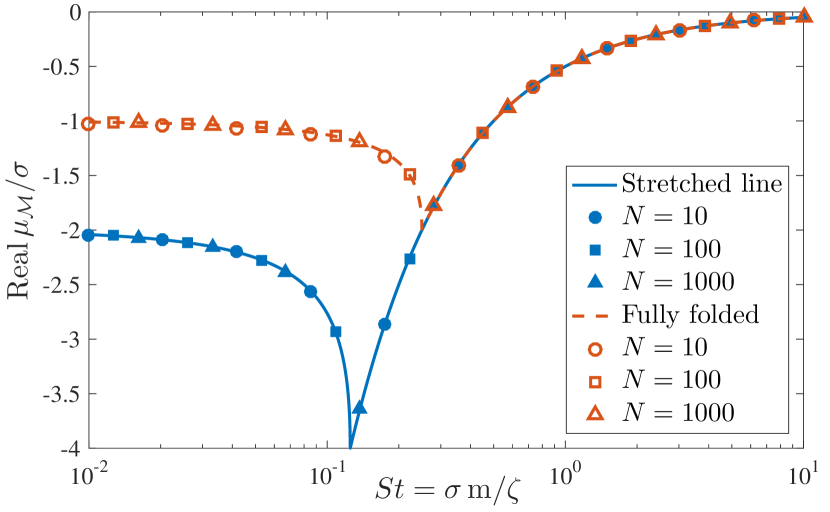
Figure 2: Real part of the most unstable eigenvalue $\mu_{\mathcal{M}}$ (in units of the fluid shear rate $\sigma$) as a function of the Stokes number $St$ for the fully stretched chain (solid line, filled symbol) and the completely folded case (dashed line, empty symbols). The lines show the predictions (see text), while symbols are numerical evaluations for various chain lengths, as labeled.

II.2.2 Folded polymer

A second stationary configuration of interest is the case when the chain is completely folded in an accordion shape. We have in that case $\varepsilon_{i}=(-1)^{i}$, so that the equations for the tensions become

$$2\lambda_{i}+\lambda_{i+1}+\lambda_{i-1}=-{\zeta\,\sigma}/{m},$$ (24)

which yields

$$\lambda_{i}=-\frac{\zeta\,\sigma}{4\,m}\left[1-(-1)^{i}\right]-\frac{\zeta\,\sigma}{4\,m}\frac{i\,(-1)^{i}}{N+1}[1+(-1)^{N}].$$ (25)

This time, the associated matrix $\bm{\Delta}_{\lambda}$ admits zero modes. Indeed, if without loss of generality we assume that $N$ is odd, the second-term in the right-hand side of (25) vanishes and the $\lambda_{i}$ alternate between $-\zeta\,\sigma/(2\,m)$ and 0. Any vector $\bm{\alpha}$ with vanishing odd components belongs to the kernel of $\bm{\Delta}_{\lambda}$. As a consequence, vectors of the form $(\bm{\alpha},\mu\,\bm{\alpha})$ are eigenvectors of $\mathcal{M}$ associated to the eigenvalue

$$\mu=\frac{\sigma}{2\,{\rm St}}\left[\sqrt{1-4\,{\rm St}}-1\right].$$

As can be seen in Fig. 2, such eigenvalues correspond to the less stable mode of this stationary configuration. As for the stretched line, a sufficiently small inertia has a stabilizing effect. The critical value is this time $1/4$, so that when ${\rm St}>1/4$, the configuration in accordion shape is as stable as the fully stretched chain.

II.2.3 Intermediate configurations

Besides these two extreme configurations, there exists in general a large number of possible stationary states, as illustrated in Fig. 3 in the over-damped (${\rm St}=0$) case for $N=20$. These various configurations where obtained numerically by a Monte–Carlo method. The fully stretched line (in the top-right corner) is in that case the most stable configuration with $\mbox{Real}\,\mu_{\mathcal{M}}=-2\,\sigma$. The fully-folded accordion shape in the bottom-left corner is associated to $\mbox{Real}\,\mu_{\mathcal{M}}=-\sigma$. Other stable configurations associated to partial foldings of the chain span the bottom half of the $(\mathcal{F},\mathcal{L})$ plane. We expect the fiber to explore them in presence of noise. This will be the case during the tumbling of the chain, as we will see later in Sec. IV.

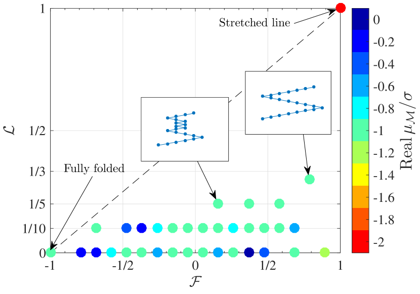
Figure 3: Stable configurations of a chain with $N=20$ and ${\rm St}=0$ in the $(\mathcal{F},\mathcal{L})$ plane. The filled circles stand for the real part of the less stable eigenvalue $\mu_{\mathcal{M}}$ (in units of $\sigma$). Two intermediate stable configurations are singled out at $\mathcal{L}\approx 1/3$, $\mathcal{F}=(N-5)/(N-1)$, where the fiber is approximately folded in three equal pieces, and at $\mathcal{L}=1/5$ and $\mathcal{F}\approx 0.15$, for which the fiber alternates between stretched and folded segments.

II.3 Numerical implementation

In the presence of noise, we simulate the dynamics of fibers by integrating numerically their equation of motion given by Eq. (4). For that purpose, we resort to an explicit first-order Euler–Maruyama method with temporal discretization. In that case, the discretized system reads:

$$\bm{V}_{i}(t+\Delta t) = \bm{V}_{i}(t)+\Delta t\left\{-(\zeta/m)\left[\bm{V}_{i}(t)-\bm{\xi}_{i}(t)\cdot\bm{\nabla}\bm{u}\right]\right.$$

$$\left.+2\lambda_{i}\,\bm{\xi}_{i}(t)-\lambda_{i+1}\,\bm{\xi}_{i+1}(t)-\lambda_{i-1}\,\bm{\xi}_{i-1}(t)\right\}$$

$$+\sqrt{\frac{2k_{\rm B}T\,\zeta}{m^{2}\ell_{\rm K}^{2}}}\,(\Delta\bm{W}_{i}-\Delta\bm{W}_{i-1}),$$

$$\bm{\xi}_{i}(t+\Delta t) = \bm{\xi}_{i}(t)+\Delta t\,\bm{V}_{i}(t),$$ (26)

where $\bm{\xi}_{i}$ is the segment labeled ’$i$’ and $\bm{V}_{i}={\rm d}\bm{\xi}_{i}/{\rm d}t$ its velocity, $\Delta t$ is the time step used in the simulation and $\Delta\bm{W}_{i}$ are the increment of a two-dimensional Wiener process over a time step $\Delta t$.

To close the system given by Eq. (26), the holonomic constraint $|\bm{\xi}_{i}(t+\Delta t)|^{2}=|\bm{\xi}_{i}(t)|^{2}$ is used to evaluate the tensions $\lambda_{i}$. Replacing with the discretized system, this constraint reads:

$$2\bm{\xi}_{i}(t)\,\cdotp\,\,\bm{V}_{i}(t)+\Delta t\left|\bm{V}_{i}(t)\right|^{2}=0.$$ (27)

This matrix equation depends non-linearly on $\bm{\xi}_{i}(t)$ and $\lambda_{i}$. As a result, there is no easy numerical resolution of the tensions $\lambda_{i}$. However, we note that tension forces have the same scaling as the stochastic term and it can be written as a series expansion in powers of $(\Delta t)^{1/2}$. This provides a new high-order method for the numerical simulation of bead-rod chains (further details are given in the Appendix).

III Coiled-stretched transition

III.1 Principle and mechanism

Fiber orientation changes constantly due to the competition between fluid stretching and thermal fluctuations. As a result, fibers explore a wide range of states and this leads to a broad distribution in the fiber length and orientation with time. In particular, a fiber can reach two notable states that are displayed in Fig. 4 for the over-damped case ${\rm St}=0$ (together with the probability density function of the fiber extension $\mathcal{L}(t)$ and orientation $\mathcal{F}(t)$):

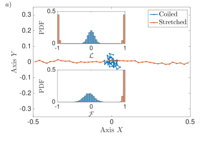
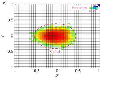
Figure 4: (color online) Extension and orientation of an elongated chain ($N=40$) at two values of Peclet numbers showing the chain in both the coiled state ($\rm Pe=0.05$) and the stretched state ($\rm Pe=0.3$). a) Snapshots of a fiber in the coiled and stretched states. The insets display the histograms of $\mathcal{L}$ and $\mathcal{F}$ for both states. b)Map showing the probability of occurrence for each discrete state in the $(\mathcal{F},\mathcal{L})$ plane around the coiled (hot color) and stretched state (cold color).

• A stretched configuration, where the fiber is oriented along the fluid streamline. This state corresponds to the case when $\rm Pe\gg 1$, i.e. when fluid stretching prevails over thermal fluctuations. The probability density function (PDF) of $\mathcal{L}(t)$ then displays a two-peak shape (around $\pm 1$ depending on the orientation of the fiber with respect to the fluid stretching). Meanwhile, the PDF of $\mathcal{F}(t)$ is peaked toward $1$ since all consecutive links are oriented in the same direction.

• A coiled configuration, where the fiber is folded several times over itself. This state occurs when $\rm Pe\ll 1$, i.e. when thermal fluctuations are predominant over fluid stretching. In that case, the PDF of $\mathcal{L}(t)$ has a Gaussian distribution with a mean value equal to $0$ (coming from the random orientation of consecutive links). In the meantime, the PDF of $\mathcal{F}(t)$ exhibit a Gaussian distribution with a mean value also equal to $0$ (due again to the random orientation of consecutive links).

Another way to differentiate between coiled and stretched states is to have a look at the fiber orientation and extension in the $(\mathcal{F},\mathcal{L})$ plane (see Fig. 4b). Fibers in the coiled state remain around the configuration $(\mathcal{F},\mathcal{L})\sim(0,0)$, whereas fibers in the stretched state are close to $(\mathcal{F},\mathcal{L})\sim(1,1)$. Figure 4b also provides additional information on the nearby partially folded/unfolded states that fibers explore. In particular, it appears that the range of nearby states accessible depends on the relative importance of thermal fluctuations to fluid stretching. This can be understood using intuitive arguments: Folding occurs thanks to thermal fluctuations and thus higher noise allows for more frequent and intense folding/unfolding events.

The Coil-Stretch (CS) transition is thus controlled by $\rm Pe$, i.e. by the balance between fluid stretching and thermal fluctuations. This transition has been extensively studied in the literature since it is key to understand the dynamics of elongated deformable particles in flows (see, e.g., Afonso and Vincenzi (2005); Ahmad and Vincenzi (2016); Ali et al. (2016); Beck and Shaqfeh (2007); De Gennes (1974); Gerashchenko et al. (2005); Kantsler and Goldstein (2012); Plan and Vincenzi (2016); Schroeder et al. (2003, 2004); Shaqfeh (2005); Watanabe and Gotoh (2010); Young and Shelley (2007)). In the following, we analyze the CS transition in the limit of very long particles with inertial effects. For that purpose, their dynamics is assessed in terms of the two observables ($\mathcal{L}$, $\mathcal{F}$) first in the overdamped case to extract the key features before characterizing how inertia affects these results.

III.2 Overdamped case

The transition from one state to another one is governed by the action of the fluid on the fiber: Coiled fibers can be stretched when fluid stretching is strong enough compared to thermal fluctuations, whereas stretched fibers can become coiled if thermal fluctuations are locally predominant. As a result, fibers orientation and extension evolve with time, going through multiple states. The transition from one state to another one is not instantaneous but occurs within a finite transition time before relaxing to a steady state. This transition time depends in a complex way on the Peclet number, the fiber length and the initial state. To compare the temporal evolution of fibers, we have characterized the fiber extension after a given time immersed in a flow (here, we have retained a time roughly equal to $10$ times the transition time). Fig 5 displays the fiber extension averaged over several realizations of the flow $\langle\mathcal{|L|}(t)\rangle_{ens}$ taken after this time. Observations that can be drawn from this plot are two-fold:

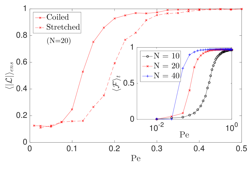
Figure 5: Fiber extension and orientation as a function of $\rm Pe$ showing the sub-critical phase transition for $N=10,20,40$. Sub-critical phase transition visible when plotting the average over several realizations of the flow $\langle\mathcal{|L|}\rangle_{ens}$. Inset showing the average orientation over time $\langle\mathcal{F}\rangle_{t}$.

• First, regardless of the initial configuration (stretched or coiled), $\langle\mathcal{|L|}\rangle_{ens}$ is characterized by a sudden increase when the Peclet number is increased. For long fibers (here $N\gtrsim 10$), a fiber is indeed stretched when fluctuations are small ($\rm Pe\gtrsim 1$) whereas it remains in a coiled state when fluctuations are large ($\rm Pe\ll 1$). Besides, the averaged value of the fiber extension $\langle\mathcal{|L|}\rangle_{ens}$ is proportional to $1/\sqrt{N}$ at small Peclet number. This can be explained using simple arguments: When thermal fluctuations are predominant over fluid stretching ($\rm Pe\ll 1$), the orientation of each elementary link is independent of its neighbors. From the Central Limit Theorem, the fiber extension $\mathcal{L}$ is converging at large $N$ toward a Gaussian with a zero mean value. We thus have $\langle\mathcal{L}\rangle_{ens}=0$, while its modulus $\langle\mathcal{|L|}\rangle_{ens}$ is proportional to $1/\sqrt{N}$.

• Second, there exists a conformation hysteresis for long fibers, meaning that the transition from the stretched state occurs at a Peclet number lower than the transition from the coiled state. There is thus a range of Peclet numbers where both states are concurrently stable to small fluctuations. This hysteresis can be interpreted as resulting from higher internal constraints found in a stretched fiber. We have indeed seen in Sec. II.2 that the tensions behave quadratically in a stretched configuration, while they are at best linear in a coiled fiber: this makes it harder to start folding a stretched fiber than to start unfolding a coiled fiber. In the hysteresis band, both states coexist since fluctuations are high enough to partially fold stretched fibers and to partially unfold coiled ones. Therefore, a large spectrum of fiber orientations and extensions can be reached in this range of Peclet numbers. This hysteresis is very similar to the hysteresis loop that has been observed for long polymers or DNA molecules in a flow Shaqfeh (2005).

To further assess the effect of $\rm Pe$ on $\mathcal{L}$ and $\mathcal{F}$, the time-averaged fiber extension and orientation has been extracted from numerical simulations when a stationary state is reached. The inset in Fig. 5 displays the orientation $\langle\mathcal{F}\rangle$ as a function of the Peclet number $\rm Pe$. It confirms that fibers are coiled for $\rm Pe\ll 1$ and stretched for $\rm Pe\gtrsim 1$. It also appears that the evolution of $\langle\mathcal{F}\rangle$ with $\rm Pe$ is monotonic: It decreases toward $0$ when $\rm Pe$ decreases. The limit at $\rm Pe\rightarrow 0$ can be understood using simple handwaving arguments: When thermal fluctuations prevails ($\rm Pe\ll 1$), the orientation of each segment is purely random and thus the probabilities for consecutive links to be either aligned or reversed is the same. As a result, the average fiber orientation $\langle\mathcal{F}\rangle$ is equal to $0$. It should be noted here that hysteresis is not visible since results have been averaged over time, i.e. the dependence on the initial conditions has been lost in the process.

Fiber orientation and extension are also affected by its length. It appears from Fig. 5 that the CS transition becomes independent of the fiber length for sufficiently large values of $N$. This can be be understood using qualitative arguments: We have seen in Sec. II.2.1 that the internal constraints within a stretched fiber have a parabolic shape with a maximum value in the middle of the fiber $\propto N^{2}$. As a result, folding around the middle of the fiber becomes harder as the fiber length $N$ increases but it remains possible to fold a long stretched fiber close to its edges or close to already folded links (where the internal constraint is smaller). Thus, when $N$ becomes large, the Stretched-to-Coil transition occurs mostly through multiple folding of the fiber around its edges or around folded links. The transition thus occurs at similar values of the Peclet number as the Coiled-to-Stretched transition, which is the exact opposite process where multiple unfolding occurs. To further confirm these trends, the fiber extension averaged over time $\langle\mathcal{|L|}\rangle_{t}$ has been characterized as a function of both $N$ and $\rm Pe$.

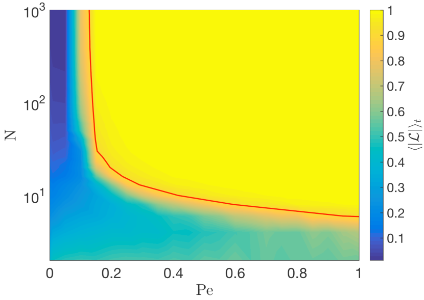
Figure 6: (color online) Average fiber extension over time $\langle\mathcal{L}\rangle_{t}$ in the $(\rm Pe,N)$ plane. The red solid line corresponds to the critical Peclet number $\rm Pe^{\star}$ at which the fiber extension exceeds a threshold $\langle\mathcal{|L|}\rangle_{t}>L^{\star}=0.9$. This shows the existence of an asymptotic regime for sufficiently long fibers.

Results are plotted in Fig. 6: One observes that a long fiber (here $N>10$) is usually coiled for $\rm Pe\lesssim 0.1$ while it remains stretched for $\rm Pe\gtrsim 0.4$. The transition between the coiled and stretched states can be distinguished using a critical Peclet number $\rm Pe^{\star}$, defined as the value at which the averaged fiber extension exceeds a certain threshold $\langle\mathcal{|L|}\rangle_{t}>L^{\star}$. The solid red line in Fig. 6 displays this critical Peclet number for $L^{\star}=0.9$. The CS transition has a non-trivial dependence on the fiber length: It becomes independent of the fiber length $N$ for sufficiently long fibers (here $N\gtrsim 30$), but it occurs at increasing Peclet numbers with small fibers (here $30\gtrsim N\gtrsim 4$).

III.3 Inertial case

We now characterize the effect of inertia on the coil/stretch transition. Drawing on the observations made in the overdamped case, we fix the fiber length to $N=20$ and characterize its orientation as a function of both $\rm Pe$ and $\rm St$. The dynamics is impacted by the inertia of each bead. In particular, two regimes can be identified depending on whether the Stokes number is greater or higher than $1/8$. Indeed, as it was shown in Sec. II.2.1 (in the absence of noise), for $\rm St<1/8$ the eigenvalues of a stretched chain are real — see Eq. (22). Therefore, at small Stokes numbers, the inertial dynamics can be seen as the one of an overdamped chain in a synthetic compressible flow where the effective compression rate reads $\sigma(1+2\,{\rm St})$.

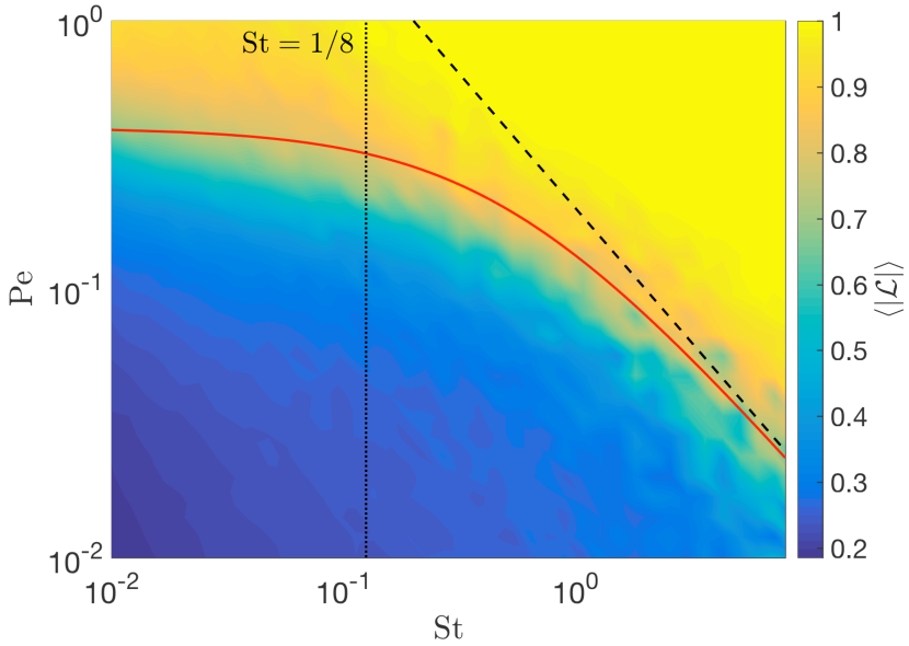
Figure 7: Time-averaged extension $\langle\mathcal{L}\rangle_{t}$ in the $(\rm St,\rm Pe)$ plane. The dotted vertical line shows the critical value ${\rm St}=1/8$. The solid and dashed lines display the prediction $\rm Pe^{\star}(\rm St)=\rm Pe^{\star}(0)/(1+2\,\rm St)$ and the asymptotic behavior $\rm Pe^{\star}(\rm St)=Pe^{\star}(0)/(2\,\rm St)$, respectively, with ${\rm Pe}^{\star}(0)=0.4$.

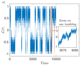
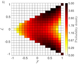
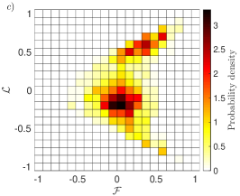
Figure 8: Evolution of the fiber orientation for $N=20$ near the CS transition (here $\rm Pe=0.14$) in the overdamped case. a) Fiber orientation $\mathcal{L}(t)$ as a function of time. Inset showing a zoom on a selected tumbling event. b) Probability of occurrence for each discrete state over the whole simulation in the $(\mathcal{F},\mathcal{L})$ plane. c) Analogous to figure b but over a selected tumbling event.

Figure 7 shows the time-averaged fiber extension $\langle\mathcal{|L|}\rangle_{t}$ in the $(\rm Pe,\rm St)$ plane. One clearly observes that for $St<1/8$, the CS transition occurs at a critical value of the Peclet number that is compatible with the formula $\rm Pe^{\star}(\rm St)=\rm Pe^{\star}(0)/(1+2\rm St)$ obtained using the effective compression rate described above. Surprisingly, this behavior describes also what is happening for $St>1/8$. At very large Stokes numbers, the critical Peclet number decreases as a power-law $\rm Pe^{\star}(\rm St)\propto\rm St^{-1}$. This can be interpreted using dimensional analysis as follows: The CS transition results from the competition between thermal fluctuations and fluid stretching and thus occurs when both contributions are balanced. According to Eq. (4), this means $1/\rm St\sim 1/(\rm Pe\,\rm St^{2})$ and thus ${\rm Pe}\sim{\rm St}^{-1}$.

IV Tumbling

IV.1 Principle and mechanism

Another typical feature of fiber dynamics is the existence of tumbling events. This is illustrated in Fig. 8a: A fiber is trapped in one of the stretched configuration with $\mathcal{L}=\pm 1$ for a long time until a sufficiently high fluctuation makes it tumble toward the stretched configuration with a reversed orientation $\mathcal{L}=\mp 1$. The inset of Fig. 8a shows a focus on one of the tumbling events: It occurs due to a favorable sequence of thermal fluctuations that allows the fiber to transition from the stretched to the coiled state, before unfolding toward the reversed stretched configuration. This process is thus very similar to the tumbling-through-folding motion that has been recently characterized for trumbbells Plan and Vincenzi (2016). It also transpires from Fig. 8a that, once the coiled state is reached, tumbling does not necessarily occur since the fiber can unfold back toward its original state. This is what happens near $t=5000$ where $\mathcal{L}$ departs from $-1$, reaches $0$, but then turns back to its earliest negative orientation.

Further information on the intermediate states explored during the tumbling event can be obtained by studying the probability of occurrence for each discrete state in the $(\mathcal{F},\mathcal{L})$ plane. This is displayed in Figs. 8b and 8c that illustrate two features of tumbling events:

• The tumbling-through-folding concept: Fibers spend most of the time close to the stretched states where $(\mathcal{F}\approx 1,\mathcal{L}\approx\pm 1)$ and tumbling events appear to take place preferentially by going through a randomly coiled state $(\mathcal{F}\approx 0,\mathcal{L}\approx 0)$. This indicates that tumbling does not correspond to a rigid flip of the fiber.

• The signature of intermediate states: The fibers seem to stay temporarily close to meta-stable states that where described in the stability analysis of Sec. II.2.3. In the present case, the state where $(\mathcal{F}\approx 0.15,\mathcal{L}\approx-0.2)$ is rather frequent during the tumbling transition. It corresponds to the partially coiled configuration shown in Fig. 3.

Tumbling is defined here as the change of the fiber extension $\mathcal{L}$ from $\pm 1$ to the opposite value. The persistence time $\tau_{t}$ corresponds to the time spend by a fiber in an extended state. In that sense, $\tau_{t}$ measures the time separating two tumbling events. As for the CS transition, tumbling has been studied previously in various flows Einarsson et al. (2016); Gustavsson et al. (2014); Parsa et al. (2012); Plan and Vincenzi (2016); Turitsyn (2007); Vincenzi (2013). We characterize here the tumbling dynamics in the case of very long fibers in terms of the two observables ($\mathcal{L}$, $\mathcal{F}$) in the overdamped case first before assessing the effect of inertia on tumbling.

IV.2 Overdamped case

As revealed by Fig. 8.a, the persistence time is distributed randomly. We have performed simulations with the same fiber length (here $N=20$) over longer times to have sufficient tumbling events to extract the PDF of $\tau_{t}$. It is plotted in Fig. 9) for various values of the Peclet number (slightly above the critical Peclet $\rm Pe^{\star}$ at which the CS transition occurs). First, it can be seen that the value of the persistence time is high, especially compared to recent experimental data on polymer dynamics in extensional flows which measured a residency time around $6s$ for a shear rate of $0.86s^{-1}$. Perkins et al. (1997). Second, the PDF turns out to have an exponential tail for large $\tau_{t}$, i.e. $p(\tau_{t})\propto\text{exp}(-\tau_{t}/\tau_{t}^{avg})$ with $\tau_{t}^{avg}$ the average persistence time. As for trumbbells in an extensional flow Plan and Vincenzi (2016), this trend can be predicted using the Freidlin–Wentzell large deviation theory Freidlin and Wentzell (1998) that characterizes the mean time required to exit from a domain due to small perturbations. Regarding tumbling as a fiber escaping from an attractor of a stochastic dynamical system in the limit of small noise, the PDF of the exit time has an exponential tail.

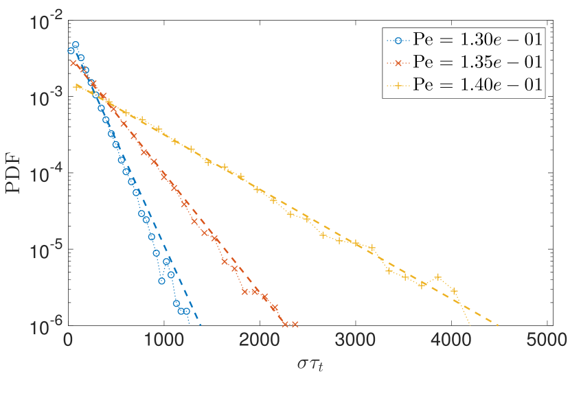
Figure 9: Probability density function (PDF) of the persistence time for $N=20$ in the overdamped case for various values of the Peclet number (slightly above the CS transition). The dotted lines correspond to the exponential law $p(\tau_{t})=\text{exp}(-\tau_{t}/\tau_{t}^{avg})/\tau_{t}^{avg}$.

Furthermore, the theory also predicts that the mean exit time increases exponentially when the amplitude of the noise decreases. This relates to the fact that it becomes harder for fibers to exit the stretched state when the amplitude of thermal fluctuations decreases. This trend is confirmed in Fig. 10, where the average persistence time is plotted as a function of the reduced Peclet number $\rm Pe^{+}=(\rm Pe-\rm Pe^{\star})/\rm Pe^{\star}$. When fluctuations are small enough (here for $\rm Pe^{+}>0.1$), one observes an exponential increase of $\langle\tau_{t}\rangle$ with $\rm Pe^{+}$. In addition, the persistence time also increases very rapidly as a function of the chain length $N$ (see the inset of Fig. 10). This means that fibers are trapped in either stretched states as $N\rightarrow\infty$ and that there is a loss of ergodicity as the fiber length diverges at a fixed Peclet number. A similar ergodicity breaking has been reported for the CS transition Beck and Shaqfeh (2007): For a fixed noise amplitude (Deborah number in the original article), the chains become kinetically trapped either in the coiled or stretched states as their length diverges. This has been explained theoretically by reducing the problem to thermally activated transitions over an energy barrier described by a rate theory. The same applies here: The energy needed for a fiber to escape from one attractor (or state) to another is proportional to the chain length, since the number of links is higher. As a result, the transition rate decays exponentially with the fiber length $N$. From a phenomenological point of view, this relates to the fact that tumbling requires a favorable sequence of thermal fluctuations to get out of the stretched state.

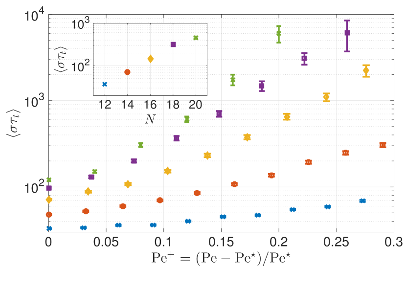
Figure 10: Average persistence time $\langle\tau_{t}\rangle$ as a function of the normalized Peclet number $\rm Pe^{+}=(\rm Pe-\rm Pe^{\star})/\rm Pe^{\star}$. Inset showing the evolution of the persistence time $\langle\tau_{t}\rangle$ with the chain length $N$.

IV.3 Inertial case

Drawing on the numerical results obtained in the overdamped case, we now characterize the effect of inertia on the tumbling dynamics of fibers. In line with the previous analysis of the CS transition including inertial effects, we have chosen to fix the fiber length to $N=20$ and to assess how the tumbling dynamics evolves with both Peclet and Stokes numbers.

The persistence time $\tau_{t}$ displays again an exponential tail at large values (see the inset in Fig. 11). The mean exit time is expected to increase exponentially as the amplitude of the noise decreases for a given value of the Stokes number. This is confirmed in Fig. 11) that displays the evolution of the persistence time as a function of the reduced Peclet number $Pe^{+}$ for three values of the Stokes number (resp. $0.1$, $0.5$ and $2$). Besides, it also appears from Fig. 11 that the persistence time increases with the Stokes number and that two regimes can be identified:

• Close to the CS transition ($\rm Pe^{+}\lesssim 0.1$), the persistence time increases linearly with the Stokes number and all curves collapse on a single master curve when plotting $\tau_{t}/\rm St$ as a function of the reduced Peclet $\rm Pe^{+}$;

• At larger Peclet numbers ($\rm Pe^{+}\gtrsim 0.1$), different behaviors are displayed by the two families of particles. Low-inertia particles ($\rm St<1/8$) appear indeed to tumble at a higher rate than high-inertia particles ($\rm St>1/8$).

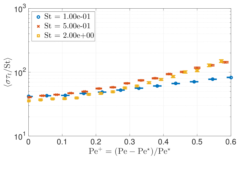
Figure 11: Average persistence time $\langle\tau_{t}\rangle$ as a function of the normalized Peclet number $\rm Pe^{+}=(\rm Pe-\rm Pe^{\star})/\rm Pe^{\star}$ for various Stokes number ($N=20$).

V Concluding remarks

The dynamics of inertial deformable chains has been explored in the case of an extensional flow. In particular, we have assessed the role of the Peclet number, Stokes number and chain length on the Coil-Stretch transition and tumbling phenomena. Numerical results have confirmed the conformation hysteresis between coiled and stretched states for sufficiently long fibers ($N\gtrsim 10$). It has also been seen that this transition depends non-linearly on these three parameters: It becomes independent of the chain length $N$ for sufficiently long fibers ($N\gtrsim 20-30$), while it evolves proportionally to $1/(1+2\rm St)$ at a given fiber size. Similarly, tumbling events have been confirmed in the case of an extensional flow close to the Coil-Stretch transition. Numerical results support recent simulations, which showed a loss of ergodicity as the chain length goes to infinity (meaning that fibers are kinetically trapped in either coiled or stretched states). The persistence time has also been shown to increase exponentially with the chain length and Peclet number, while it increases non-linearly with the Stokes number.

These promising results on the dynamics of inertial chains in an extensional flow call for further refinements and developments. In particular, it is worth assessing how 3D simulations affect these results and to see if recent results showing a higher tendency for trumbbells to remain in the stretched state in 3D cases than in 2D cases are confirmed. The next step will be to investigate the role of fiber flexibility on the coil-stretch transition and on tumbling dynamics. Another question remains to be explored: What is happening when fluctuations are triggered by the flow itself rather than by noise. This issue will be investigated by coupling the dynamics of such fibers with turbulent velocity gradients (coming directly from direct numerical simulations). The role of fluctuations both in the intensity of the velocity gradient and in its direction will be explored. In the general context of fibers in turbulent flows, further studies are needed to evaluate the effect of preferential sampling and preferential concentration of such fibers in the near-wall region especially in the case of highly elongated and deformable fibers. These issues will be probed in future studies by coupling the dynamics of such fibers with direct simulations of wall-bounded turbulent flows.

VI Acknowledgments

This work has been supported by the French government, through the Investments for the Future project UCA^JEDI managed by the National Research Agency (ANR) with the reference number ANR-15-IDEX-01. The work of C.H. was supported by the PRESTIGE Program (grant PRESTIGE-2017-1-0025) coordinated by Campus France. Through this PRESTIGE program, this research has received funding from the People Program (Marie Curie Actions) of the European Union’s Seventh Framework Program (FP7/2007-2013) under REA grant agreement n. PCOFUND-GA-2013-609102. C.H. acknowledges the support of the EU COST Action MP1305 “Flowing Matter”.

Appendix A Appendix

A.1 Appendix 1: implementation in the general case

In the following, we focus on the numerical implementation of the fiber equation of motion in an extensional flow. In that case, it is given by Eq. 4 which can be re-written as:

$$\frac{{\rm d}\bm{\xi}_{i}}{{\rm d}t} = {\bm{V}}_{i}$$ (28)

$$\frac{{\rm d}\bm{V}_{i}}{{\rm d}t} = -\frac{\zeta}{m}\left[\bm{V}_{i}-\bm{\xi}_{i}\cdot\bm{\nabla}\bm{u}\right]+\sqrt{\frac{2k_{\rm B}T\,\zeta}{m^{2}\ell_{\rm K}^{2}}}\,(\bm{\eta}_{i}-\bm{\eta}_{i-1})$$ (29)

$$+2\lambda_{i}\,\bm{\xi}_{i}-\lambda_{i+1}\,\bm{\xi}_{i+1}-\lambda_{i-1}\,\bm{\xi}_{i-1},$$

This equation is solved using a simple first order Euler–Maruyama method with temporal discretization (time step $\Delta t$):

$$\bm{V}_{i}(t+\Delta t) = \bm{V}_{i}(t)+\delta\bm{V}_{i}(t)$$

$$\bm{\xi}_{i}(t+\Delta t) = \bm{\xi}_{i}(t)+\Delta t\,\bm{V}_{i}(t)$$ (30)

with the variation of the bead velocity given by:

$$\delta\bm{V}_{i}(t) = -\Delta t\,\frac{\zeta}{m}\left[\bm{V}_{i}(t)-\bm{\xi}_{i}(t)\cdot\bm{\nabla}\bm{u}\right]$$ (31)

$$+\sqrt{\Delta t}\,K_{Br}(\bm{\gamma}_{i}-\bm{\gamma}_{i-1})-\Delta t\,(\Delta_{\xi}\,\bm{\lambda})_{i}$$

with $K_{Br}=\sqrt{2k_{\rm B}T\,\zeta}/(m\,\ell_{\rm K})$ the diffusion coefficient for Brownian motion, $\gamma_{i}$ taken from a Gaussian distribution (with zero mean and a standard deviation equal to $1$), $\bm{\lambda}$ denotes the $N$-dimensional vector $(\lambda_{1},\dots,\lambda_{N})^{\mathsf{T}}$, and ${\bm{\Delta}}_{\xi}$ is such that $(\bm{\Delta}_{\xi}\,\bm{\lambda})_{i}=-2\lambda_{i}\bm{\xi}_{i}+\lambda_{i-1}\bm{\xi}_{i-1}+\lambda_{i+1}\bm{\xi}_{i+1}$.

The tension forces acting on each rigid segment is obtained by imposing a constant distance between consecutive beads $\left|\bm{\xi}_{i}(t+\Delta t)\right|^{2}=\left|\bm{\xi}_{i}(t)\right|^{2}$ for all $1\leq i\leq N$. Using Eq. (30), this leads to

$$2\bm{\xi}_{i}(t)\cdotp\bm{V}_{i}(t)+\Delta t\left|\bm{V}_{i}(t)\right|^{2}=0.$$ (32)

By writing the above equation at time $t+\Delta t$, we obtain

$$2\,\Delta t\,\left|\bm{V}_{i}(t)\right|^{2}+2\,\bm{\xi}_{i}(t)\cdotp\delta\bm{V}_{i}(t)$$

$$+4\,\Delta t\,\bm{V}_{i}(t)\cdotp\delta\bm{V}_{i}(t)+\Delta t\,\left|\delta\bm{V}_{i}(t)\right|^{2} =0$$ (33)

The above non-linearities does not allow for writing an explicit solution. Yet, one can note that the terms on the left-hand side involve various powers of the time step $\Delta t$. For that reason, we chose to decompose the tensions $\lambda_{i}$ as series in powers of $\sqrt{\Delta t}$, i.e.

$$\Delta t\,\bm{\lambda}=\sum_{k=1}^{\infty}\bm{\lambda}^{(k)}\,\Delta t^{k/2}.$$ (34)

The series starts with terms $\mathcal{O}(\sqrt{\Delta t})$ to account for the tension that balances the noise. We can then identify each contribution to obtain a set of equations for each term:

• Terms in $\Delta t^{1/2}$:

  $$\bm{\xi}_{i}\cdotp(\bm{\Delta}_{\xi}\bm{\lambda}^{(1)})_{i}=K_{Br}\,\bm{\xi}_{i}\cdotp(\bm{\gamma}_{i}-\bm{\gamma}_{i-1}).$$

• Terms in $\Delta t$

  $$\bm{\xi}_{i}\cdotp(\bm{\Delta}_{\xi}\bm{\lambda}^{(2)})_{i}=\left|\bm{V}_{i}\right|^{2}-\frac{\zeta}{m}\bm{\xi}_{i}\cdotp\left(\bm{V}_{i}-\bm{\xi}_{i}\cdot\bm{\nabla}\bm{u}\right).$$

• Terms in $\Delta t^{3/2}$

  $$\bm{\xi}_{i}\cdotp(\bm{\Delta}_{\xi}\bm{\lambda}^{(3)})_{i}=2\bm{V}_{i}\cdotp\left[K_{Br}\,(\bm{\gamma}_{i}-\bm{\gamma}_{i-1})-(\bm{\Delta}_{\xi}\bm{\lambda}^{(1)})_{i}\right].$$

• Terms in $\Delta t^{2}$

  $$\bm{\xi}_{i}\cdotp(\bm{\Delta}_{\xi}\bm{\lambda}^{(4)})_{i} = 2\bm{V}_{i}\cdotp\left[-\frac{\zeta}{m}\bm{\xi}_{i}\cdotp\left(\bm{V}_{i}-\bm{\xi}_{i}\cdot\bm{\nabla}\bm{u}\right)-(\bm{\Delta}_{\xi}\bm{\lambda}^{(2)})_{i}\right]$$

  $$+\frac{1}{2}\left|K_{Br}\,(\bm{\gamma}_{i}-\bm{\gamma}_{i-1})-(\bm{\Delta}_{\xi}\bm{\lambda}^{(1)})_{i}\right|^{2}.$$

The above expansion can be continued to reach an arbitrary precision. In practice, we stop at a given order and use the corresponding approximation of the tensions to update the fiber velocity. In the paper, we used the expansion to order $\Delta t$. The terms order $\Delta t^{3/2}$ are stochastic with a zero mean, so that the error is in average $\mathcal{O}(\Delta t^{2})$.

A.2 Appendix 2: implementation for small fibers

In the case of fibers composed of beads that act as tracers in the flow, the equation of motion simplifies to:

$$\frac{{\rm d}\bm{\xi}_{i}}{{\rm d}t} = \bm{\xi}_{i}\cdot\bm{\nabla}\bm{u}+\sqrt{\frac{2k_{\rm B}T}{\ell_{\rm K}^{2}\,\zeta}}\,(\bm{\eta}_{i}-\bm{\eta}_{i-1})$$ (35)

$$+2\lambda_{i}^{\prime}\,\bm{\xi}_{i}-\lambda_{i+1}^{\prime}\,\bm{\xi}_{i+1}-\lambda_{i-1}^{\prime}\,\bm{\xi}_{i-1},$$

with $\lambda^{\prime}=\lambda\,{m}/{\zeta}$. This equation is solved using a first order Euler–Maruyama method with time step $\Delta t$:

$$\bm{\xi}_{i}(t+\Delta t) = \bm{\xi}_{i}(t)+\delta\bm{\xi}_{i}(t)$$ (36)

with the variation of the bead position $\delta\bm{\xi}_{i}(t)$ given by:

$$\delta\bm{\xi}_{i}(t)= \Delta t\,\bm{\xi}_{i}(t)\cdot\bm{\nabla}\bm{u}+\sqrt{\Delta t}\,K_{Br}^{\prime}(\bm{\gamma}_{i}-\bm{\gamma}_{i-1})$$ (37)

$$-\Delta t\,(\Delta_{\xi}\,\bm{\lambda}^{\prime})_{i}$$

with $K_{Br}^{\prime}=\sqrt{(2k_{\rm B}T)/\,(\zeta\,\ell_{\rm K}^{2})}$ the diffusion coefficient for Brownian motion, the $\gamma_{i}$’s taken from a Gaussian distribution (with zero mean and a standard deviation $1$).

The tension forces acting on each rigid segment are obtained by imposing a constant distance between consecutive beads, i.e. $\left|\bm{\xi}_{i}(t+\Delta t)\right|^{2}=\left|\bm{\xi}_{i}(t)\right|^{2}$, leading to

$$2\bm{\xi}_{i}(t)\cdotp\delta\bm{\xi}_{i}(t)+\left|\delta\bm{\xi}_{i}(t)\right|^{2}=0$$ (38)

As in the inertial case, we decompose the tensions $\lambda_{i}^{\prime}$ as

$$\Delta t\,\bm{\lambda}^{\prime}=\sum_{k=1}^{\infty}\bm{\lambda}^{\prime(k)}\,\Delta t^{k/2},$$ (39)

and identify contributions of different orders in $\Delta t^{1/2}$:

• Terms in $\Delta t^{1/2}$:

  $$\bm{\xi}_{i}\cdotp(\Delta_{\xi}\,\bm{\lambda}^{\prime(1)})_{i}=K_{Br}^{\prime}\,\bm{\xi}_{i}\cdotp(\bm{\gamma}_{i}-\bm{\gamma}_{i-1}).$$

• Terms in $\Delta t$:

  $$\bm{\xi}_{i} \cdotp(\Delta_{\xi}\,\bm{\lambda}^{\prime(2)})_{i}=\bm{\xi}_{i}\cdotp\left(\bm{\xi}_{i}\cdotp\bm{\nabla}\bm{u}\right)-K_{Br}^{\prime}(\bm{\gamma}_{i}-\bm{\gamma}_{i-1})\cdotp(\Delta_{\xi}\,\bm{\lambda}^{\prime(1)})_{i}$$

  $$+\frac{1}{2}\left|K_{Br}^{\prime}(\bm{\gamma}_{i}-\bm{\gamma}_{i-1})\right|^{2}+\frac{1}{2}\left|(\Delta_{\xi}\,\bm{\lambda}^{\prime(1)})_{i}\right|^{2}.$$

• Terms in $\Delta t^{3/2}$

  $$\bm{\xi}_{i} \cdotp(\Delta_{\xi}\,\bm{\lambda}^{\prime(3)})_{i}=\left(\bm{\xi}_{i}\cdotp\bm{\nabla}\bm{u}-(\Delta_{\xi}\,\bm{\lambda}^{\prime(2)})_{i}\right)$$

  $$\,\cdotp\left(K_{Br}^{\prime}(\bm{\gamma}_{i}-\bm{\gamma}_{i-1})-(\Delta_{\xi}\,\bm{\lambda}^{\prime(1)})_{i}\right).$$

• Terms in $\Delta t^{2}$

  $$\bm{\xi}_{i} \cdotp(\Delta_{\xi}\,\bm{\lambda}^{\prime(4)})_{i}=-\left(\bm{\xi}_{i}\cdotp\bm{\nabla}\bm{u}\right)\cdotp(\Delta_{\xi}\,\bm{\lambda}^{\prime(2)})_{i}$$

  $$\left((\Delta_{\xi}\,\bm{\lambda}^{\prime(1)})_{i}-K_{Br}^{\prime}(\bm{\gamma}_{i}-\bm{\gamma}_{i-1})\right)\cdotp(\Delta_{\xi}\,\bm{\lambda}^{\prime(3)})_{i}$$

  $$+\frac{1}{2}\left|\bm{\xi}_{i}\cdotp\bm{\nabla}\bm{u}\right|^{2}+\frac{1}{2}\left|(\Delta_{\xi}\,\bm{\lambda}^{\prime(2)})_{i}\right|^{2}.$$

The above approximation, with terms up to those of order $\Delta t^{2}$, is used in the paper.

References

- Lundell et al. (2011) F. Lundell, L. D. Söderberg, and P. H. Alfredsson, Annual Review of Fluid Mechanics 43, 195 (2011).
- Cui and Grace (2007) H. Cui and J. R. Grace, International Journal of Multiphase Flow 33, 921 (2007).
- Shaqfeh (2005) E. S. Shaqfeh, Journal of Non-Newtonian Fluid Mechanics 130, 1 (2005).
- Jumars et al. (2009) P. A. Jumars, J. H. Trowbridge, E. Boss, and L. Karp-Boss, Marine Ecology 30, 133 (2009).
- Young et al. (2012) A. M. Young, L. Karp-Boss, P. Jumars, and E. Landis, Limnology and Oceanography 57, 1789 (2012).
- Pruppacher et al. (1998) H. R. Pruppacher, J. D. Klett, and P. K. Wang, “Microphysics of clouds and precipitation,” (1998).
- Lindner and Shelley (2015) A. Lindner and M. Shelley, in Fluid-Structure Interactions in Low-Reynolds-Number Flows, Vol. 168 (2015) pp. 168–192.
- Voth and Soldati (2017) G. A. Voth and A. Soldati, Annual Review of Fluid Mechanics 49, 249 (2017).
- Pumir and Wilkinson (2011) A. Pumir and M. Wilkinson, New journal of physics 13, 093030 (2011).
- Parsa et al. (2012) S. Parsa, E. Calzavarini, F. Toschi, and G. A. Voth, Physical Review Letters 109, 134501 (2012).
- Vincenzi (2013) D. Vincenzi, Journal of Fluid Mechanics 719, 465 (2013).
- Gustavsson et al. (2014) K. Gustavsson, J. Einarsson, and B. Mehlig, Physical review letters 112, 014501 (2014).
- Gupta et al. (2014) A. Gupta, D. Vincenzi, and R. Pandit, Physical Review E 89, 021001 (2014).
- Chevillard and Meneveau (2013) L. Chevillard and C. Meneveau, Journal of Fluid Mechanics 737, 571 (2013).
- Gustavsson and Biferale (2016) K. Gustavsson and L. Biferale, Physical Review Fluids 1, 054201 (2016).
- Musacchio and Vincenzi (2011) S. Musacchio and D. Vincenzi, Journal of Fluid Mechanics 670, 326 (2011).
- Plan and Vincenzi (2016) E. L. C. V. M. Plan and D. Vincenzi, in Proc. R. Soc. A, Vol. 472 (The Royal Society, 2016) p. 20160226.
- Ali et al. (2016) A. Ali, E. L. C. V. M. Plan, S. S. Ray, and D. Vincenzi, Physical Review Fluids 1, 082402 (2016).
- Brouzet et al. (2014) C. Brouzet, G. Verhille, and P. Le Gal, Physical review letters 112, 074501 (2014).
- Perkins et al. (1994) T. T. Perkins, D. E. Smith, S. Chu, et al., Science-AAAS-Weekly Paper Edition-including Guide to Scientific Information 264, 819 (1994).
- Perkins et al. (1995) T. T. Perkins, D. E. Smith, R. G. Larson, and S. Chu, Science 268, 83 (1995).
- Verhille and Bartoli (2016) G. Verhille and A. Bartoli, Experiments in Fluids 57, 1 (2016).
- Kantsler and Goldstein (2012) V. Kantsler and R. E. Goldstein, Phys. Rev. Lett. 108, 038103 (2012).
- Hsiao et al. (2017) K.-W. Hsiao, C. Sasmal, J. Ravi Prakash, and C. M. Schroeder, Journal of Rheology 61, 151 (2017).
- Harasim et al. (2013) M. Harasim, B. Wunderlich, O. Peleg, M. Kröger, and A. R. Bausch, Physical review letters 110, 108302 (2013).
- Liu and Steinberg (2010) Y. Liu and V. Steinberg, EPL (Europhysics Letters) 90, 44005 (2010).
- Chertkov (2000) M. Chertkov, Physical review letters 84, 4761 (2000).
- López et al. (2015) H. López, J.-P. Hulin, H. Auradou, and M. D’Angelo, Physics of Fluids 27, 013102 (2015).
- Strelnikova et al. (2017) N. Strelnikova, M. Göllner, and T. Pfohl, Macromolecular Chemistry and Physics 218 (2017).
- Cruz et al. (2012) C. Cruz, F. Chinesta, and G. Regnier, Archives of Computational Methods in Engineering 19, 227 (2012).
- Larson (2005) R. G. Larson, Journal of Rheology 49, 1 (2005).
- Underhill and Doyle (2004) P. T. Underhill and P. S. Doyle, Journal of non-newtonian fluid mechanics 122, 3 (2004).
- Kratky and Porod (1949) O. Kratky and G. Porod, Recueil des Travaux Chimiques des Pays-Bas 68, 1106 (1949).
- Bird et al. (1987) R. B. Bird, C. R. Curtiss, R. C. Armstrong, and O. Hassager, (1987).
- Marchioli et al. (2010) C. Marchioli, M. Fantoni, and A. Soldati, Physics of fluids 22, 033301 (2010).
- Mortensen et al. (2008) P. Mortensen, H. Andersson, J. Gillissen, and B. Boersma, Physics of Fluids 20, 093302 (2008).
- Puliafito and Turitsyn (2005) A. Puliafito and K. Turitsyn, Physica D 211, 9 (2005).
- Kramers (1944) H. Kramers, Physica 11, 1 (1944).
- Beck and Shaqfeh (2007) V. A. Beck and E. S. Shaqfeh, Journal of Rheology 51, 561 (2007).
- Rouse Jr (1953) P. E. Rouse Jr, The Journal of Chemical Physics 21, 1272 (1953).
- Afonso and Vincenzi (2005) M. M. Afonso and D. Vincenzi, Journal of Fluid Mechanics 540, 99 (2005).
- Ahmad and Vincenzi (2016) A. Ahmad and D. Vincenzi, Physical Review E 93, 052605 (2016).
- De Gennes (1974) P. De Gennes, The Journal of Chemical Physics 60, 5030 (1974).
- Gerashchenko et al. (2005) S. Gerashchenko, C. Chevallard, and V. Steinberg, EPL (Europhysics Letters) 71, 221 (2005).
- Schroeder et al. (2003) C. M. Schroeder, H. P. Babcock, E. S. Shaqfeh, and S. Chu, Science 301, 1515 (2003).
- Schroeder et al. (2004) C. M. Schroeder, E. S. Shaqfeh, and S. Chu, Macromolecules 37, 9242 (2004).
- Watanabe and Gotoh (2010) T. Watanabe and T. Gotoh, Physical Review E 81, 066301 (2010).
- Young and Shelley (2007) Y.-N. Young and M. J. Shelley, Phys. Rev. Lett. 99, 058303 (2007).
- Einarsson et al. (2016) J. Einarsson, B. Mihiretie, A. Laas, S. Ankardal, J. Angilella, D. Hanstorp, and B. Mehlig, Physics of Fluids 28, 013302 (2016).
- Turitsyn (2007) K. Turitsyn, Journal of Experimental and Theoretical Physics 105, 655 (2007).
- Perkins et al. (1997) T. T. Perkins, D. E. Smith, and S. Chu, Science 276, 2016 (1997).
- Freidlin and Wentzell (1998) M. I. Freidlin and A. D. Wentzell, in Random Perturbations of Dynamical Systems (Springer, 1998) pp. 15–43.