Matrix Group Integrals, Surfaces, and Mapping Class Groups I: $\mathcal{U}\left(n\right)$

Abstract

Since the 1970’s, physicists and mathematicians who study random matrices in the GUE or GOE models are aware of intriguing connections between integrals of such random matrices and enumeration of graphs on surfaces. We establish a new aspect of this theory: for random matrices sampled from the group $\mathcal{U}\left(n\right)$ of unitary matrices.

More concretely, we study measures induced by free words on $\mathcal{U}\left(n\right)$. Let $\mathrm{\mathbf{F}}_{r}$ be the free group on $r$ generators. To sample a random element from $\mathcal{U}\left(n\right)$ according to the measure induced by $w\in\mathrm{\mathbf{F}}_{r}$, one substitutes the $r$ letters in $w$ by $r$ independent, Haar-random elements from $\mathcal{U}\left(n\right)$. The main theme of this paper is that every moment of this measure is determined by families of pairs $\left(\Sigma,f\right)$, where $\Sigma$ is an orientable surface with boundary, and $f$ is a map from $\Sigma$ to the bouquet of $r$ circles, which sends the boundary components of $\Sigma$ to powers of $w$. A crucial role is then played by Euler characteristics of subgroups of the mapping class group of $\Sigma$.

As corollaries, we obtain asymptotic bounds on the moments, we show that the measure on $\mathcal{U}\left(n\right)$ bears information about the number of solutions to the equation $\left[u_{1},v_{1}\right]\cdots\left[u_{g},v_{g}\right]=w$ in the free group, and deduce that one can “hear” the stable commutator length of a word through its unitary word measures.

1 Introduction

Let $\mathcal{U}\left(n\right)$ denote the group of $n\times n$ unitary complex matrices, and let $\mathrm{\mathbf{F}}_{r}$ denote the free group on $r$ generators with fixed basis (free generating set) $B=\left\{x_{1},\ldots,x_{r}\right\}$. For a word $w\in\mathrm{\mathbf{F}}_{r}$, we define the $w$-measure on $\mathcal{U}\left(n\right)$ as the push-forward of the Haar measure on $\mathcal{U}\left(n\right)^{r}$ through the word map $w\colon\mathcal{U}\left(n\right)^{r}\to\mathcal{U}\left(n\right)$. In plain terms, assume that $w=x_{i_{1}}^{\varepsilon_{1}}\cdots x_{i_{m}}^{\varepsilon_{m}}$. To sample a random element from $\mathcal{U}\left(n\right)$ by the $w$-measure, sample $r$ independent Haar-random elements $A_{1},\ldots,A_{r}\in\mathcal{U}\left(n\right)$ and evaluate $w\left(A_{1},\ldots,A_{r}\right)=A_{i_{1}}^{\varepsilon_{1}}\cdots A_{i_{m}}^{\varepsilon_{m}}\in\mathcal{U}\left(n\right)$.

The motivation to study $w$-measures on unitary groups or on compact groups in general originates in questions revolving around random walks on these groups, in the study of representation varieties, in problems in the theory of Free Probability, and in challenges in the study of free groups. However, as the current paper shows, the study of $w$-measures is interesting for its own sake and reveals deep and surprising connections with other mathematical concepts. See also [PP15].

Expected trace

We study word measures by considering their moments, and more particularly the expected product of traces. For every $\ell\in\mathbb{N}_{\geq 1}$ and $w_{1},\ldots,w_{\ell}\in\mathrm{\mathbf{F}}_{r}$, consider the quantity

$${\cal T}r_{w_{1},\ldots,w_{\ell}}\left(n\right)\stackrel{{\scriptstyle\mathrm{def}}}{{=}}\int_{A_{1},\ldots,A_{r}\in\mathcal{U}\left(n\right)}\mathrm{tr}\left(w_{1}\left(A_{1},\ldots,A_{r}\right)\right)\cdot\ldots\cdot\mathrm{tr}\left(w_{\ell}\left(A_{1},\ldots,A_{r}\right)\right)d\mu$$ (1.1)

where $A_{1},\ldots,A_{r}\in\mathcal{U}\left(n\right)$ are independent Haar-random unitary matrices. The development of “Weingarten calculus” for computing integrals on $\mathcal{U}\left(n\right)$ [Wei78, Xu97, Col03, CŚ06] leads readily to the following result:

Proposition 1.1.

Let $\ell\in\mathbb{N}_{\geq 1}$ and $w_{1},\ldots,w_{\ell}\in\mathrm{\mathbf{F}}_{r}$. Then for large enough $n$, the quantity ${\cal T}r_{w_{1},\ldots,w_{\ell}}\left(n\right)$ is given by a rational expression in $n$ with rational coefficients, namely, by an element of $\mathbb{Q}\left(n\right)$.

Here “large enough $n$” means that $n\geq\max_{x\in B}L_{x}$, where $L_{x}$ is the total number of instances of $x^{+1}$ in the words $w_{1},\ldots,w_{\ell}$.

In Section 2 we give explicit combinatorial formulas for ${\cal T}r_{w_{1},\ldots,w_{\ell}}\left(n\right)$, and the main innovation here is the emergence of surfaces in these formulas. In Table 1 we list some examples for these rational expressions for concrete words.

$\ell$	$w_{1},\ldots,w_{\ell}$	${\cal T}r_{w_{1},\ldots,w_{\ell}}\left(n\right)$	Laurent Series
1	$\left[x,y\right]$	$\frac{1}{n}$	$\frac{1}{n}$
	$\left[x^{3},y\right]$	$\frac{3}{n}$	$\frac{3}{n}$
	$\left[x,y\right]^{2}$	$\frac{-4}{n^{3}-n}$	$\frac{-4}{n^{3}}+\frac{-4}{n^{5}}+\frac{-4}{n^{7}}+\cdots$
	$\left[x,y\right]^{3}$	$\frac{9\left(n^{2}+4\right)}{n^{5}-5n^{3}+4n}$	$\frac{9}{n^{3}}+\frac{81}{n^{5}}+\frac{369}{n^{7}}+\cdots$
	$\left[x,y\right]\left[x,z\right]$	$0$	$0$
	$\left[x,y\right]\left[x,z\right]\left[x,t\right]$	$0$	$0$
2	$x^{2}y^{2},xy^{-3}x^{-3}y$	$\frac{4\left(n^{2}-5\right)}{n^{4}-5n^{2}+4}$	$\frac{4}{n^{2}}+\frac{0}{n^{4}}+\frac{-16}{n^{6}}+\frac{-80}{n^{8}}+\cdots$
	$w,w^{-1}$ for $w=x^{2}yxy^{-1}$	$1$	$1$
	$w,w^{-1}$ for $w=x^{2}y^{2}xy^{-1}$	$\frac{n^{4}-5n^{2}}{n^{4}-5n^{2}+4}$	$1+\frac{0}{n^{2}}+\frac{-4}{n^{4}}+\frac{-20}{n^{6}}+\cdots$

Table 1: Some examples for the rational expression for ${\cal T}r_{w_{1},\ldots,w_{\ell}}\left(n\right)$ and (the beginning of) its Laurent series expansion. All these examples contain words in $\mathrm{\mathbf{F}}_{4}$ with generators $\left\{x,y,z,t\right\}$. The notation $\left[x,y\right]$ is for the commutator $xyx^{-1}y^{-1}$ .

The main theme of the current paper is the interpretation of these expressions for ${\cal T}r_{w_{1},\ldots,w_{\ell}}\left(n\right)$ in terms of properties of $w$. We explain their degree and their leading coefficient. More generally, we show how the entire Laurent series for ${\cal T}r_{w_{1},\ldots,w_{\ell}}\left(n\right)$ is determined by natural objects related to $w_{1},\ldots,w_{\ell}$.

Extending maps from circles to surfaces

Our main result, Theorem 1.7 below, states that the expressions for ${\cal T}r_{w_{1},\ldots,w_{\ell}}\left(n\right)$ can be described in terms of certain surfaces and maps. Roughly, consider a bouquet of $r$ circles ${\textstyle\bigvee^{r}S^{1}}$ with fundamental group identified with $\mathrm{\mathbf{F}}_{r}$. Now consider $\ell$ disjoint circles (one-spheres) $C_{1},\ldots,C_{\ell}$ and a map

$$f_{w_{1},\ldots,w_{\ell}}\colon C_{1}\sqcup\ldots\sqcup C_{\ell}\to{\textstyle\bigvee^{r}S^{1}}$$

sending $C_{i}$ to a loop at the bouquet representing $w_{i}$. We now construct pairs $\left(\Sigma,f\right)$ of an orientable surface $\Sigma$ with $\ell$ boundary components together with a map $f\colon\Sigma\to{\textstyle\bigvee^{r}S^{1}}$, so that the restriction of $f$ to the boundary $\partial\Sigma$ is equal to $f_{w_{1},\ldots,w_{\ell}}$. From this set one can fully recover the expressions for ${\cal T}r_{w_{1},\ldots,w_{\ell}}\left(n\right)$. See Figure 1.1.

Figure 1.1: Two surfaces extending the map from three circles to ${\textstyle\bigvee^{r}S^{1}}$ corresponding to the triple of words $w_{1},w_{2},w_{3}$.

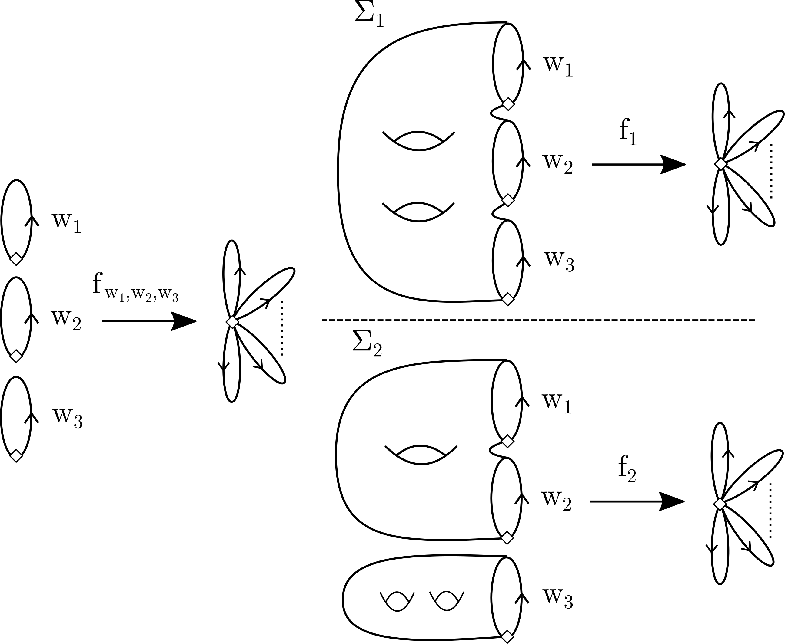
More formally, identify the free group $\mathrm{\mathbf{F}}_{r}$ with the fundamental group of ${\textstyle\bigvee^{r}S^{1}}$, by orienting every circle in the bouquet and determining a bijection between the circles and the generators $x_{1},\ldots,x_{r}$ of $\mathrm{\mathbf{F}}_{r}$. Mark the wedge point by $o$. We have

$$\mathrm{\mathbf{F}}_{r}\cong\pi_{1}\left({\textstyle\bigvee^{r}S^{1}},o\right).$$

Let $C_{1}\sqcup\ldots\sqcup C_{\ell}$ be a disjoint union of $\ell$ oriented 1-spheres with a marked point $v_{i}\in C_{i}$ for every $i=1,\ldots,\ell$. The map $f_{w_{1},\ldots,w_{\ell}}\colon C_{1}\sqcup\ldots\sqcup C_{\ell}\to{\textstyle\bigvee^{r}S^{1}}$ sends $v_{1},\ldots,v_{\ell}$ to $o$, and the induced map on fundamental groups sends the loop at $v_{i}$ around the oriented $C_{i}$ to $\left[w_{i}\right]$.

Definition 1.2.

Let $\Sigma$ be a surface with $\ell$ boundary components $\partial\Sigma_{1},\ldots,\partial\Sigma_{\ell}$ and a marked point $v_{i}\in\partial\Sigma_{i}$ in each boundary component. Let $f\colon\Sigma\to{\textstyle\bigvee^{r}S^{1}}$ be a map to the bouquet. We say that $\left(\Sigma,f\right)$ is admissible for $w_{1},\ldots,w_{\ell}\in\mathrm{\mathbf{F}}_{r}$ if the following two conditions hold:

1. $\Sigma$ is oriented and compact, with no closed connected components.

2. The restriction of $f$ to the boundary of $\Sigma$ is homotopic to $f_{w_{1},\ldots,w_{\ell}}$ relative to the marked points $v_{1},\ldots,v_{\ell}$. Namely, for every $i=1,\ldots,\ell$,

   $$f_{*}\left(\left[\overrightarrow{\partial_{i}\Sigma}\right]\right)=w_{i}\in\pi_{1}\left({\textstyle\bigvee^{r}S^{1}},o\right),$$

   where $\overrightarrow{\partial_{i}\Sigma}$ is the closed loop at $v_{i}$ around $\partial_{i}\Sigma$ with orientation induced from the orientation of $\Sigma$.

In particular, we assume in the above definition that $f\left(v_{i}\right)=o$ for every $i=1,\ldots,\ell$.

There is a natural equivalence relation between different admissible pairs: first, if $f_{1},f_{2}\colon\Sigma\to{\textstyle\bigvee^{r}S^{1}}$ are homotopic relative to the marked points $v_{1},\ldots,v_{\ell}$, then we think of $\left(\Sigma,f_{1}\right)$ and $\left(\Sigma,f_{2}\right)$ as equivalent. We denote by $\left[f\right]$ the homotopy class of $f$ relative to $v_{1},\ldots,v_{\ell}$. Second, there is a natural action of $\mathrm{MCG}\left(\Sigma\right)$, the mapping class group of $\Sigma$, on homotopy classes of maps $\Sigma\to{\textstyle\bigvee^{r}S^{1}}$, and we define different maps in the same orbit to be equivalent (see Definition 1.3). Here, $\mathrm{MCG}\left(\Sigma\right)$ is defined as the group of homeomorphisms of $\Sigma$ which fix the boundary $\partial\Sigma$ pointwise, modulo such homeomorphisms which are isotopic to the identity. The action of $\mathrm{MCG}\left(\Sigma\right)$ on homotopy classes of maps

$$\left\{\left[f\right]\,\middle|\,\left(\Sigma,f\right)\leavevmode\nobreak\ \mathrm{admissible\leavevmode\nobreak\ for}\leavevmode\nobreak\ w_{1},\ldots,w_{\ell}\right\}$$

is by precomposition: the action of $\left[\rho\right]\in\mathrm{MCG}\left(\Sigma\right)$ on $\left[f\right]$ results in $\left[f\circ\rho^{-1}\right]$. We gather these considerations in the following definition:

Definition 1.3.

Let $\left(\Sigma,f\right)$ and $\left(\Sigma^{\prime},f^{\prime}\right)$ be admissible for $w_{1},\ldots,w_{\ell}$. They are equivalent, denoted $\left(\Sigma,f\right)\sim\left(\Sigma^{\prime},f^{\prime}\right)$, if there is an orientation preserving homeomorphism $\rho\colon\Sigma\to\Sigma^{\prime}$, such that for every $i=1,\ldots,\ell$, $\rho\left(v_{i}\right)=v_{i}^{\prime}$ and $f\simeq f^{\prime}\circ\rho$ are homotopic relative to the marked points $v_{1},\ldots v_{\ell}$. We denote by $\left[\left(\Sigma,f\right)\right]$ the equivalence class of $\left(\Sigma,f\right)$. We denote the set of equivalence classes by $\mathsf{Surfaces}\left(w_{1},\ldots,w_{\ell}\right)$:

$$\mathsf{Surfaces}\left(w_{1},\ldots,w_{\ell}\right)\stackrel{{\scriptstyle\mathrm{def}}}{{=}}\left\{\left[\left(\Sigma,f\right)\right]\,\middle|\,\left(\Sigma,f\right)\leavevmode\nobreak\ \mathrm{is\leavevmode\nobreak\ admissible\leavevmode\nobreak\ for}\leavevmode\nobreak\ w_{1},\ldots,w_{\ell}\right\}.$$

The main goal of this paper is to show how one can read the terms of the Laurent series of ${\cal T}r_{w_{1},\ldots,w_{\ell}}\left(n\right)$ from this set $\mathsf{Surfaces}\left(w_{1},\ldots,w_{\ell}\right)$ of equivalence classes of pairs of surfaces and maps.

The $L^{2}$-Euler characteristic of stabilizers

The Laurent series of ${\cal T}r_{w_{1},\ldots,w_{\ell}}\left(n\right)$ gets some contribution from every $\left[\left(\Sigma,f\right)\right]\in\mathsf{Surfaces}\left(w_{1},\ldots,w_{\ell}\right)$. As stated in Theorem 1.7 below, this contribution is of the form $c\cdot n^{\alpha}$, where $c$ and $\alpha$ are integers. The order of magnitude of the contribution is controlled by the Euler characteristic of the surface: $\alpha=\chi\left(\Sigma\right)$. However, to determine the integer coefficient $c$, an important role is played by the stabilizer of $\left[f\right]$ under the action of $\mathrm{MCG}\left(\Sigma\right)$, which we denote by $\mathrm{MCG}\left(f\right)$:

$$\mathrm{MCG}\left(f\right)\stackrel{{\scriptstyle\mathrm{def}}}{{=}}\mathrm{MCG}\left(\Sigma\right)_{\left[f\right]}.$$

Note that by definition, the elements of $\mathrm{MCG}\left(\Sigma\right)$ permute homotopy classes of maps inside the same equivalence class $\left[\left(\Sigma,f\right)\right]$. Yet, occasionally, they may stabilize $\left[f\right]$, in the sense that $f\circ\rho$ and $f$ are homotopic relative to $v_{1},\ldots,v_{\ell}$. Given the class $\left[\left(\Sigma,f\right)\right]$, the stabilizer $\mathrm{MCG}\left(f\right)$ is defined up to conjugation.

The actual invariant of the stabilizer that appears in the contribution of $\left[\left(\Sigma,f\right)\right]$ to ${\cal T}r_{w_{1},\ldots,w_{\ell}}\left(n\right)$ is its $L^{2}$-Euler characteristic. The $L^{2}$-Euler characteristic of a group is defined for groups with nice enough properties and can take any real value. It is the alternating sum of the von Neumann dimensions of the homology groups of a natural chain complex of modules over the group von Neumann algebra, as we explain in more detail in Section 4.1 below, and see [Lüc02]. Thus, to state our main result, we first need the following auxiliary theorem which is interesting for its own sake.

Theorem 1.4.

Let $\Sigma$ be a compact orientable surface with no closed connected components. Let $f\colon\Sigma\to{\textstyle\bigvee^{r}S^{1}}$ be a map. Then the stabilizer $\mathrm{MCG}\left(f\right)=\mathrm{MCG}\left(\Sigma\right)_{\left[f\right]}$ has a well-defined $L^{2}$-Euler characteristic. Moreover, this $L^{2}$-Euler Characteristic is an integer.

Note that in the statement of the theorem it does not matter whether $\left[f\right]$ is the homotopy class of $f$ relative to $\partial\Sigma$ or relative to some marked points in every boundary component - this nuance does not modify the action of $\mathrm{MCG}\left(\Sigma\right)$ on the homotopy classes of maps.

Theorem 1.4 can be strengthened in an important special case we now introduce:

Definition 1.5.

A null-curve of $\left(\Sigma,f\right)$ is a non-nullhomotopic simple closed curve $\gamma$ in $\Sigma$ with $f\left(\gamma\right)$ nullhomotopic in ${\textstyle\bigvee^{r}S^{1}}$. A pair $\left(\Sigma,f\right)$ is called incompressible if it admits no null-curves. It is called compressible otherwise.

If $\left(\Sigma,f\right)$ is admissible for $w_{1},\ldots,w_{\ell}$ and is compressible, then one can cut $\Sigma$ along a null-curve, fill the two new boundary components with discs to obtain $\Sigma^{\prime}$ and extend $f$ to a map $f^{\prime}\colon\Sigma^{\prime}\to{\textstyle\bigvee^{r}S^{1}}$. If $\Sigma^{\prime}$ contains a closed component, remove it to obtain $\Sigma^{\prime\prime}$ and let $f^{\prime\prime}$ denote the restriction of $f^{\prime}$ to $\Sigma^{\prime\prime}$. The new pair $\left(\Sigma^{\prime\prime},f^{\prime\prime}\right)$ is admissible for $w_{1},\ldots,w_{\ell}$ and satisfies $\chi\left(\Sigma^{\prime\prime}\right)\geq\chi\left(\Sigma^{\prime}\right)=\chi\left(\Sigma\right)+2$, as the possibly closed component of $\Sigma^{\prime}$ cannot be a sphere. Thus, pairs $\left(\Sigma,f\right)$ with $\Sigma$ having maximal Euler characteristic are necessarily incompressible. When $f$ is incompressible we have the following stronger version of Theorem 1.4:

Theorem 1.6.

Let $\Sigma$ be a compact orientable surface with boundary in every connected component, and let $f\colon\Sigma\to{\textstyle\bigvee^{r}S^{1}}$ be incompressible. Then the stabilizer

$$\Gamma=\mathrm{MCG}\left(f\right)=\mathrm{MCG}\left(\Sigma\right)_{\left[f\right]}$$

admits a finite simplicial complex as a $K\left(\Gamma,1\right)$-space. In particular, $\Gamma$ has a well-defined Euler characteristic in the ordinary sense, which coincides with its $L^{2}$-Euler characteristic.

Main result

Our main theorem shows that the Laurent expansion of ${\cal T}r_{w_{1},\ldots,w_{\ell}}\left(n\right)$ is given by Euler characteristics of both the stabilizers of maps in $\mathsf{Surfaces}\left(w_{1},\ldots,w_{\ell}\right)$ and also the Euler characteristics of the surfaces. When the $L^{2}$-Euler characteristic of a group $\Gamma$ is defined, we denote it by $\chi^{\left(2\right)}\left(\Gamma\right)$.

Theorem 1.7 (Main Theorem).

Let $w_{1},\ldots,w_{\ell}\in\mathrm{\mathbf{F}}_{r}$. For large enough $n$,

$${\cal T}r_{w_{1},\ldots,w_{\ell}}\left(n\right)=\sum_{\left[\left(\Sigma,f\right)\right]\in\mathsf{Surfaces}\left(w_{1},\ldots,w_{\ell}\right)}\chi^{\left(2\right)}\left(\mathrm{MCG}\left(f\right)\right)\cdot n^{\chi\left(\Sigma\right)}.$$ (1.2)

Indeed, for any given exponent $\chi_{0}$, there are only finitely many non-zero terms of order $n^{\chi_{0}}$, namely, the set

$$\left\{\left[\left(\Sigma,f\right)\right]\in\mathsf{Surfaces}\left(w_{1},\ldots,w_{\ell}\right)\leavevmode\nobreak\ \,\middle|\leavevmode\nobreak\ \,\chi\left(\Sigma\right)=\chi_{0}\leavevmode\nobreak\ \mathrm{and}\leavevmode\nobreak\ \chi^{\left(2\right)}\left(\mathrm{MCG}\left(f\right)\right)\neq 0\right\}$$

is finite.

The last statement of the theorem explains why the theorem yields a well-defined coefficient for every term in the Laurent series of ${\cal T}r_{w_{1},\ldots,w_{\ell}}\left(n\right)$. However, we do not know yet how to derive from this theorem the rationality of ${\cal T}r_{w_{1},\ldots,w_{\ell}}\left(n\right)$, which we prove directly using Weingarten calculus - see Proposition 1.1 and Section 2. This rationality means that in a way we do not yet fully understand, the $L^{2}$-Euler characteristics of different pairs $\left[\left(\Sigma,f\right)\right]\in\mathsf{Surfaces}\left(w_{1},\ldots,w_{\ell}\right)$ “know about each other” – see Question 4 in Section 6.

As an immediate corollary of Proposition 1.1 and Theorem 1.7, we get an asymptotic upper bound on ${\cal T}r_{w_{1},\ldots,w_{\ell}}\left(n\right)$. Denote

$$\chi_{\max}\left(w_{1},\ldots,w_{\ell}\right)\stackrel{{\scriptstyle\mathrm{def}}}{{=}}\max\left\{\chi\left(\Sigma\right)\,\middle|\,\left[\left(\Sigma,f\right)\right]\in\mathsf{Surfaces}\left(w_{1},\ldots,w_{\ell}\right)\right\},$$

where $\chi_{\max}\left(w_{1},\ldots,w_{\ell}\right)=-\infty$ if $\mathsf{Surfaces}\left(w_{1},\ldots,w_{\ell}\right)$ is empty, which is equivalent to $w_{1}\cdots w_{\ell}\notin\left[\mathrm{\mathbf{F}}_{r},\mathrm{\mathbf{F}}_{r}\right]$ - see Claims 2.1 and 2.12. A well-known fact going back at least to Culler [Cul81, Paragraph 1.1] is that $\mathrm{chi}\left(w\right)=1-2\cdot\mathrm{cl}\left(w\right)$, where $\mathrm{cl}\left(w\right)$ is the commutator length of $w$, defined as

$$\mathrm{cl}\left(w\right)\stackrel{{\scriptstyle\mathrm{def}}}{{=}}\min\left\{g\,\middle|\,w=\left[u_{1},v_{1}\right]\cdots\left[u_{g},v_{g}\right]\leavevmode\nobreak\ \mathrm{with}\leavevmode\nobreak\ u_{i},v_{i}\in\mathrm{\mathbf{F}}_{r}\right\}.$$

Thus,

Corollary 1.8.

Let $w_{1},\ldots,w_{\ell}\in\mathrm{\mathbf{F}}_{r}$. Then

$${\cal T}r_{w_{1},\ldots,w_{\ell}}\left(n\right)=O\left(n^{\chi_{\max}\left(w_{1},\ldots,w_{\ell}\right)}\right).$$ (1.3)

In particular, for $w\in\mathrm{\mathbf{F}}_{r}$,

$${\cal T}r_{w}\left(n\right)=O\left(n^{\chi_{\max}\left(w\right)}\right)=O\left(\frac{1}{n^{2\cdot{\cal\mathrm{cl}}\left(w\right)-1}}\right).$$ (1.4)

Remark 1.9.

Recall that the Euler characteristic of an orientable compact surface of genus-$g$ and $\ell$ boundary components is $2-2g-\ell$. Thus, Theorem 1.7 yields that the Laurent series of ${\cal T}r_{w_{1},\ldots,w_{\ell}}\left(n\right)$ is supported on odd (respectively even) powers of $n$ if $\ell$ is odd (respectively even). This is a nice interpretation of a fact that can also be derived directly from analysis involving Weingarten calculus.

Algebraic interpretation

The connection between the commutator length of a word $w$ and $\chi_{\max}\left(w\right)$ led to the algebraic interpretation (1.4) in Corollary 1.8. This algebraic perspective also gives an interesting interpretation to our main theorem. Because a connected surface $\Sigma$ is a $K\left(\pi_{1}\left(\Sigma\right),1\right)$-space, the Dehn-Nielsen-Baer Theorem states there is a natural isomorphism between $\mathrm{MCG}\left(\Sigma\right)$ and a certain subgroup of $\mathrm{Aut}\left(\pi_{1}\left(\Sigma\right)\right)$ (see, for example, [FM12, Chapter 8] for its version for closed surfaces, and [MP15, Thm 2.4]). For example, if $\Sigma_{g,1}$ is a connected genus $g$ surface with one boundary component, then $\pi_{1}\left(\Sigma\right)\cong\mathrm{\mathbf{F}}_{2g}=\mathrm{\mathbf{F}}\left(a_{1},b_{1},\ldots,a_{g},b_{g}\right)$, and $\mathrm{MCG}\left(\Sigma\right)$ is isomorphic to the stabilizer of $\left[a_{1},b_{1}\right]\cdots\left[a_{g},b_{g}\right]$ in $\mathrm{Aut}\left(\mathrm{\mathbf{F}}_{2g}\right)$ – stabilizing this element reflects the fact that mapping classes in $\mathrm{MCG}\left(\Sigma\right)$ fix the boundary of $\Sigma_{g,1}$.

Along these lines, the set $\mathsf{Surfaces}\left(w\right)$ can be interpreted as equivalence classes of solutions to the equations

$$\left[u_{1},v_{1}\right]\cdots\left[u_{g},v_{g}\right]=w$$ (1.5)

with $u_{i},v_{i}\in\mathrm{\mathbf{F}}_{r}$ and varying $g$, where the equivalence relation is given by the action of the stabilizer $\mathrm{Aut}\left(\mathrm{\mathbf{F}}_{2g}\right)_{\left[a_{1},b_{1}\right]\cdots\left[a_{g},b_{g}\right]}$. In particular, the pairs $\left[\left(\Sigma,f\right)\right]\in\mathsf{Surfaces}\left(w\right)$ with maximal $\chi\left(\Sigma\right)$ correspond to equivalence classes of solutions to (1.5) with $g={\cal\mathrm{cl}}\left(w\right)$ minimal. Often, these solutions have trivial stabilizers, in which case $\chi^{\left(2\right)}\left(\mathrm{MCG}\left(f\right)\right)=1$. For example, the stabilizer is trivial if the solutions consist of $2g$ free words, or, equivalently, if $f\colon\Sigma\to{\textstyle\bigvee^{r}S^{1}}$ is $\pi_{1}$-injective – see Lemma 5.1. Thus, one could say

• “The leading coefficient of ${\cal T}r_{w}(n)$ counts the number of equivalence classes of solutions to (1.5) with  $g={\cal\mathrm{cl}}\left(w\right)$, up to corrections for the existence of non-trivial stabilizers.”

Examples

Let us now illustrate Theorem 1.7 and Corollary 1.8 on some of the examples from Table 1. The techniques by which we obtain some of the details in the following cases are explained throughout the paper, especially in Section 5.2.

• The commutator length of $w=\left[x,y\right]$ is obviously one, and there is a single equivalence class of solutions to the equation $\left[u,v\right]=w$, or, equivalently, a single element $\left[\left(\Sigma,f\right)\right]\in\mathsf{Surfaces}\left(w\right)$ with $\chi\left(\Sigma\right)=\chi_{\max}\left(w\right)=-1$. The stabilizer $\mathrm{MCG}\left(f\right)$ is trivial and so the first term in the Laurent expansion of ${\cal T}r_{\left[x,y\right]}\left(n\right)$ is $\frac{1}{n}$. Every other element $\left[\left(\Sigma,f\right)\right]\in\mathsf{Surfaces}\left(w\right)$ has $\chi\left(\Sigma\right)\leq-3$ and $\chi^{\left(2\right)}\left(\mathrm{MCG}\left(f\right)\right)=0$.

• We have ${\cal\mathrm{cl}}\left(\left[x^{3},y\right]\right)=1$. There are exactly three in-equivalent solutions to $\left[u,v\right]=w$: $\left[x^{3},y\right]$, $\left[x^{3},yx\right]$ and $\left[x^{3},yx^{2}\right]$. In contrast, the solution $\left[x^{3},yx^{3}\right]$ is equivalent to $\left[x^{3},y\right]$ because the automorphism of $\mathrm{\mathbf{F}}_{2}=\mathrm{\mathbf{F}}\left(a,b\right)$ fixing $a$ and mapping $b\to ba$, stabilizes $\left[a,b\right]$. In this case, all three solutions have trivial stabilizers, hence the leading term of ${\cal T}r_{\left[x^{3},y\right]}$ is $\frac{3}{n}$. It seems like there are no other elements of $\mathsf{Surfaces}\left(\left[x^{3},y\right]\right)$ with non-vanishing $\chi^{\left(2\right)}\left(\mathrm{MCG}\left(f\right)\right)$ (at least there are none with $\chi\left(\Sigma\right)\geq-7$).

• In general, if ${\cal\mathrm{cl}}\left(w\right)=1$, then every solution to $\left[u,v\right]=w$ has trivial stabilizer, because $u$ and $v$ are necessarily free words inside $\mathrm{\mathbf{F}}_{r}$ (namely, $\left\langle u,v\right\rangle\cong\mathrm{\mathbf{F}}_{2}$). Thus, for words of commutator length one we have ${\cal T}r_{w}\left(n\right)=\frac{K}{n}+O\left(\frac{1}{n^{3}}\right)$, where $K$ is the number of equivalence classes of ways to write $w$ as a commutator. Likewise, every solution to (1.5) with $\left\langle u_{1},v_{1},\ldots,u_{g},v_{g}\right\rangle\cong\mathrm{\mathbf{F}}_{2g}$ has a trivial stabilizer – see Lemma 5.1.

• For $w=\left[x,y\right]^{2}$ we have ${\cal\mathrm{cl}}\left(w\right)=2$. There is a single equivalence class of solutions to (1.5) with $g=2$, and $\mathrm{MCG}\left(f\right)\cong\mathrm{\mathbf{F}}_{5}$. As a bouquet of five circles is a $K\left(\mathrm{\mathbf{F}}_{5},1\right)$-space, we have $\chi\left(\mathrm{\mathbf{F}}_{5}\right)=-4$. This explains the leading term of ${\cal T}r_{\left[x,y\right]^{2}}$.

• The somewhat surprising fact that ${\cal\mathrm{cl}}\left(\left[x,y\right]^{3}\right)=2$ was pointed out in [Cul81]. (Interestingly, Culler shows in that paper that ${\cal\mathrm{cl}}\left(\left[x,y\right]^{n}\right)=\left\lfloor\frac{n}{2}\right\rfloor+1$.) For example, $\left[x,y\right]^{3}=\left[xyx^{-1},y^{-1}xyx^{-2}\right]\left[y^{-1}xy,y^{2}\right]$. There are nine in-equivalent solutions in this case, each with a trivial stabilizer. This explain the leading term $\frac{9}{n^{3}}$. There is a single pair $\left[\left(\Sigma,f\right)\right]\in\mathsf{Surfaces}\left(\left[x,y\right]^{3}\right)$ with $\chi\left(\Sigma\right)=-5$ and $\chi^{\left(2\right)}\left(\mathrm{MCG}\left(f\right)\right)\neq 0$. The stabilizer in this single pair satisfies $\chi^{\left(2\right)}\left(\mathrm{MCG}\left(f\right)\right)=81$. This explain the term $\frac{81}{n^{5}}$.

• The word $w=\left[x,y\right]\left[x,z\right]$ has ${\cal\mathrm{cl}}\left(w\right)=2$ and admits a single solution to (1.5) with $g=2$. The stabilizer of this solution is isomorphic to $\mathbb{Z}$ and $\chi^{\left(2\right)}\left(\mathbb{Z}\right)=\chi\left(\mathbb{Z}\right)=0$. Note that this explains why the coefficient of $n^{-3}$ vanishes, but not why ${\cal T}r_{w}\left(n\right)=0$.

• The word $w=\left[x,y\right]\left[x,z\right]\left[x,t\right]$ has ${\cal\mathrm{cl}}\left(w\right)=3$ and admits a single solution to (1.5) with $g=3$. The stabilizer of this solution is isomorphic to $\mathbb{Z}\times\mathrm{\mathbf{F}}_{2}$ and $\chi^{\left(2\right)}\left(\mathbb{Z}\times\mathrm{\mathbf{F}}_{2}\right)=\chi\left(\mathbb{Z}\times\mathrm{\mathbf{F}}_{2}\right)=0$ (consult [MP15, Page 59] for more details).

• For $w_{1}=x^{2}y^{2}$ and $w_{2}=xy^{-3}x^{-3}y$ we have $\chi_{\max}\left(w_{1},w_{2}\right)=-2$. There are four $\left[\left(\Sigma,f\right)\right]\in\mathsf{Surfaces}\left(w_{1},w_{2}\right)$ with $\chi\left(\Sigma\right)=-2$, each with a trivial stabilizer, hence the leading term $\frac{4}{n^{2}}$. All $\chi\left(\Sigma\right)=-4$ solutions have $\chi^{\left(2\right)}\left(\mathrm{MCG}\left(f\right)\right)=0$, while there is a single solution with non-vanishing contribution and $\chi\left(\Sigma\right)=-6$, for which $\chi^{\left(2\right)}\left(\mathrm{MCG}\left(f\right)\right)=-16$.

• For every $w\neq 1$, $\chi_{\max}\left(w,w^{-1}\right)=0$ because there is an obvious annulus in $\mathsf{Surfaces}\left(w,w^{-1}\right)$. In both examples of this sort in Table 1, there is a single such annulus, and with a trivial stabilizer, hence the leading term $1$. In both cases there are no other incompressible pairs in $\mathsf{Surfaces}\left(w,w^{-1}\right)$, but while for $w=x^{2}yxy^{-1}$, it seems that every compressible pair has vanishing contribution to ${\cal T}r_{w,w^{-1}}\left(n\right)$, for $w=x^{2}y^{2}xy^{-1}$ there is a compressible pair $\left[\left(\Sigma,f\right)\right]$ with $\chi\left(\Sigma\right)=-4$ and $\chi^{\left(2\right)}\left(\mathrm{MCG}\left(f\right)\right)=-4$.

Compressible vs. incompressible pairs $\left[\left(\Sigma,f\right)\right]\in\mathsf{Surfaces}\left(w_{1},\ldots,w_{\ell}\right)$

The difference between compressible and incompressible pairs $\left[\left(\Sigma,f\right)\right]\in\mathsf{Surfaces}\left(w_{1},\ldots,w_{\ell}\right)$ is already apparent from the fact that Theorem 1.6, or at least its proof, apply only to the incompressible case. The crucial property of incompressible pairs will be pointed out in Section 4.4 in the sequel of the paper. But there are some further differences we point out here.

First, there are finitely many incompressible elements in $\mathsf{Surfaces}\left(w_{1},\ldots,w_{\ell}\right)$ – see Corollary 2.14. Because highest-Euler-characteristic elements are always incompressible, we deduce there are finitely many elements $\left[\left(\Sigma,f\right)\right]\in\mathsf{Surfaces}\left(w_{1},\ldots,w_{\ell}\right)$ with $\chi\left(\Sigma\right)=\chi_{\max}\left(w_{1},\ldots,w_{\ell}\right)$. In addition, as the examples above illustrate, the stabilizer $\mathrm{MCG}\left(f\right)$ of an incompressible solution is often trivial.

In contrast, there are infinitely many compressible elements in $\mathsf{Surfaces}\left(w_{1},\ldots,w_{\ell}\right)$. In fact, there are often even infinitely many compressible elements $\left[\left(\Sigma,f\right)\right]$ with $\chi\left(\Sigma\right)=\chi_{0}$ for a given non-maximal $\chi_{0}$, namely, for $\chi_{0}=\chi_{\max}\left(w_{1},\ldots,w_{\ell}\right)-2k$ with $k\in\mathbb{Z}_{\geq 1}$, although, as stated in Theorem 1.7, almost all of them have zero contribution to ${\cal T}r_{w_{1},\ldots,w_{\ell}}\left(n\right)$. Moreover, the stabilizer of a compressible pair is never trivial: a Dehn twist along a null-curve is a non-trivial element in the stabilizer.

1.1 Related lines of work

The evaluation of the integrals in (1.1) is a fundamental issue relating to several different areas of mathematics.

I. Matrix integrals in Gaussian models

The connection between the enumeration of graphs on surfaces and matrix integrals in the classical GUE, GOE and GSE models was first established by ’t Hooft [tH74] and later rediscovered by Harer and Zagier [HZ86]. For example, let $\mathrm{GUE}\left(n\right)$ denote the probability space of $n\times n$ Hermitian complex matrices endowed with complex Gaussian measure on each entry, where the $\left(i,j\right)$ entry is independent of all other entries except for $\left(j,i\right)$. The following equation [LZ04, Proposition 3.3.1] illustrates this connection:

$$\mathbb{E}_{H\in\mathrm{GUE}\left(n\right)}\left[\left(\mathrm{tr}H\right)^{\alpha_{1}}\left(\mathrm{tr}H^{2}\right)^{\alpha_{2}}\cdots\left(\mathrm{tr}H^{k}\right)^{\alpha_{k}}\right]=\sum_{\sigma}n^{F\left(\sigma\right)}.$$ (1.6)

The summation on the right hand side is over ribbon graphs (also known as fat-graphs) with $\alpha_{i}$ vertices of degree $i$ for $i=1,\ldots,k$, where $\sigma$ is a perfect matching of the half-edges emanating from these vertices. The exponent $F\left(\sigma\right)$ is the number of faces in the embedding of the resulting ribbon graph on the surface of smallest possible genus. We stress that (1.6) is only an illustration of the theory, and there are many generalizations (e.g., for integrals over tuples of independent Hermitian matrices) and deep applications. For an excellent presentation of this theory, we refer the reader to [LZ04, Chapter 3].

There are many similarities between this by-now classical theory and the theory we develop in the current paper. For example, apart from the natural emergence of surfaces, the combinatorial formulas for ${\cal T}r_{w_{1},\ldots,w_{\ell}}\left(n\right)$ we develop in Section 2 also involve a summation over perfect matchings. In addition, these matrix integrals over $\mathrm{GUE}$ were used, inter alia, to compute the Euler characteristic of the mapping class group of closed surfaces with punctures [HZ86, Pen88]. In fact, these Euler characteristics appear as coefficients in certain generating functions for integrals as in (1.6) (e.g., [Pen88, Theorem 1.1 and Corollary 3.1]).

There are also substantial differences. Among others, $\mathcal{U}\left(n\right)$ being a group endowed with Haar measure means that integrals as in (1.6) over a single Haar-random element can be completely computed using theoretical properties of the Haar measure, as was done in [DS94], and the computation becomes more interesting when multiple random elements are involved. It also means that word-measure on $\mathcal{U}\left(n\right)$ have nice properties, such as being $\mathrm{Aut}\left(\mathrm{\mathbf{F}}_{r}\right)$-invariant, as explained in the following paragraph. In addition, the crucial role played here by maps from the surfaces to the bouquet of circles is completely absent in the classical theory. Another difference is that the summation in the right hand side of (1.6) is finite, with the exponents increasing as the Euler characteristic of the surface decreases. The best analogue in the current paper (2.10) involves an infinite summation with exponents decreasing together with the Euler characteristic of the surfaces. Finally, there is also a big difference in the role played by Euler characteristics of (subgroups of) the mapping class groups of surfaces.

II. Word measures on groups

The same way $w\in\mathrm{\mathbf{F}}_{r}$ induces a measure on $\mathcal{U}\left(n\right)$, it also induces a probability measure on any compact group (consult [HLS15] for recent results and references concerning the image of the word map $w\colon G^{r}\to G$ on compact Lie groups including $\mathcal{U}\left(n\right)$). By showing that Nielsen moves on $w$ do not affect the resulting word measure, it is easy to see that two words in the same $\mathrm{Aut}\left(\mathrm{\mathbf{F}}_{r}\right)$-orbit in $\mathrm{\mathbf{F}}_{r}$ induce the same measure on every compact group (see [MP15, Section 2.2] for a proof). But is this the only reason for two words to have such a strong connection? A version of the following conjecture appears, for example, in [AV11, Question 2.2] and in [Sha13, Conjecture 4.2].

Conjecture 1.10.

If two words $w_{1},w_{2}\in\mathrm{\mathbf{F}}_{r}$ induce the same measure on every compact group, then there exists $\phi\in\mathrm{Aut}\left(\mathrm{\mathbf{F}}_{r}\right)$ with $w_{2}=\phi\left(w_{1}\right)$.

A special case of this conjecture deals with the $\mathrm{Aut}\left(\mathrm{\mathbf{F}}_{r}\right)$-orbit of the single-letter word $x_{1}$, namely, with the set of primitive words. Several researchers have asked whether words inducing the Haar measure on every compact group are necessarily primitive. This was settled to the affirmative in [PP15, Theorem 1.1] using word measures on symmetric groups. In subsequent work [MP19b], we use the results in this paper and, mainly, Corollary 1.8, to prove that if a word $w$ induces the same measure as $u_{g}=\left[x_{1},y_{1}\right]\cdots\left[x_{g},y_{g}\right]$ on every compact group then $w=\phi\left(u_{g}\right)$ for some $\phi\in\mathrm{Aut}\left(\mathrm{\mathbf{F}}_{r}\right)$.

Short of proving Conjecture 1.10, one could hope to collect as many invariants of words as possible that can be determined by word measures induced on groups. For example, ${\cal\mathrm{cl}}\left(w\right)$, the commutator length of a word, and more generally, $\chi_{\max}\left(w_{1},\ldots,w_{\ell}\right)$, the highest possible Euler characteristic of a surface in $\mathsf{Surfaces}\left(w_{1},\ldots,w_{\ell}\right)$, play an important role in our results. However, because the coefficient of $n^{\chi_{\max}\left(w_{1},\ldots,w_{\ell}\right)}$ in ${\cal T}r_{w_{1},\ldots,w_{\ell}}\left(n\right)$ occasionally vanishes, it is not clear whether ${\cal\mathrm{cl}}\left(w\right)$ or $\chi_{\max}\left(w_{1},\ldots,w_{\ell}\right)$ are determined by word measures on $\mathcal{U}\left(n\right)$.

In contrast, the measures do determine a related number, the stable commutator length of $w$. This algebraic quantity is defined by

$$\mathrm{scl}(w)\equiv\lim_{m\to\infty}\frac{{\cal\mathrm{cl}}(w^{m})}{m}.$$ (1.7)

(There is an analogous definition for finite sets of words.) There is a deep theory behind this invariant, and for background we refer to the short survey [Cal08] and long one [Cal09a] by Calegari. Relying on the rationality result of Calegari [Cal09b] that shows, in particular, that $\mathrm{scl}$ takes on rational values in $\mathrm{\mathbf{F}}_{r}$, we are able to show the following:

Corollary 1.11.

The stable commutator length of a word $w\in\left[\mathrm{\mathbf{F}}_{r},\mathrm{\mathbf{F}}_{r}\right]$ can be determined by the measures it induces on unitary groups in the following way:

$$\mathrm{scl}\left(w\right)=\inf_{\ell>0;\,j_{1},\ldots,j_{\ell}>0}\frac{-\lim_{n\to\infty}\log_{n}\left|{\cal T}r_{w^{j_{1}},\ldots,w^{j_{\ell}}}\left(n\right)\right|}{2\left(j_{1}+\ldots+j_{\ell}\right)}.$$ (1.8)

A similar result is true for the stable commutator length of several words. We explain how Corollary 1.11 follows from Theorem 1.7 and Calegari’s rationality theorem in Section 5.1.

Remark 1.12.

In fact, with regards to Conjecture 1.10, word-measures on $\mathcal{U}\left(n\right)$ alone do not suffice and Conjecture 1.10 is not true if “every compact group” is replaced by “$\mathcal{U}\left(n\right)$ for all $n$”. Indeed, for every $w\in\mathrm{\mathbf{F}}_{r}$ and every $n$, the $w$-measure on $\mathcal{U}\left(n\right)$ is identical to the $w^{-1}$-measure. However, in general, $w$ and $w^{-1}$ belong to two different $\mathrm{Aut}\left(\mathrm{\mathbf{F}}_{r}\right)$-orbits. See also Question 1 in Section 6.

III. Harmonic analysis on representation varieties.

The integral in (1.1) can be viewed as an integral over the space of representations $\mathrm{Hom}\left(\mathrm{\mathbf{F}}_{r},\mathcal{U}(n)\right)$ and in fact, as an integral over the representation variety

$$\mathrm{Rep}\left(\mathrm{\mathbf{F}}_{r},\mathcal{U}(n)\right)=\mathrm{Hom}\left(\mathrm{\mathbf{F}}_{r},\mathcal{U}(n)\right)/\mathcal{U}(n)$$

since the functions $\mathrm{tr}\circ w_{i}$ are invariant under $\mathcal{U}(n)$-conjugation, and so is the Haar measure. More generally, if $\Sigma_{g}$ is the closed genus $g$ surface, then the spaces $\mathrm{Rep}\left(\pi_{1}\left(\Sigma_{g}\right),\mathcal{U}(n)\right)$ are of interest in geometry, via ‘Higher Teichmüller theory’, dynamics as pioneered by Goldman [Gol97], and mathematical physics [Wit91]. For an overview see [Lab13]. For any closed curve on the surface, there is a natural function (Wilson loop) on the representation variety, given by the trace of the image of that curve in a given representation. It is natural to ask what is the integral of this function with respect to the volume form given by the Atiyah-Bott-Goldman symplectic structure on $\mathrm{Rep}\left(\pi_{1}\left(\Sigma_{g}\right),\mathcal{U}(n)\right)$ [AB83, Gol84]. Our work answers this question for representations of free groups.

IV. Free probability theory.

Voiculescu proved in [Voi91, Theorem 3.8] that for $w\neq 1$,

$${\cal T}r_{w}(n)=o(1),\quad n\to\infty.$$ (1.9)

This is referred to the asymptotic *-freeness of the non-commutative independent random variables $\left(u_{1},\ldots,u_{r}\right)\in\mathcal{U}\left(n\right)^{r}$, meaning that in the limit they can be modeled by the “Free Probability Theory” developed by Voiculescu (see, for example, the monograph [VDN92]). Such asymptotic freeness results are known for broad families of ensembles, including general Gaussian random matrices (due to Voiculescu in the same paper [Voi91, Theorem 2.2]). In later works (1.9) is strengthened to ${\cal T}r_{w}\left(n\right)=O\left(\frac{1}{n}\right)$ whenever $w\neq 1$ [MŚS07, Răd06]. Our work gives quantitative bounds on the decay rate of ${\cal T}r_{w}(n)$ (in many cases, from above and below) - see Corollary 1.8.

More generally, free probabilists are interested in the limit of ${\cal T}r_{w_{1},\ldots,w_{\ell}}\left(n\right)$ as $n\to\infty$. This is given by the following corollary of our main result, which is essentially [MŚS07, Theorem 2] and [Răd06, Theorem 4.1]:

Corollary 1.13.

Let $w_{1},\ldots,w_{\ell}\in\mathrm{\mathbf{F}}_{r}$, each not equal to $1$, and write $w_{i}=u_{i}^{d_{i}}$ where $u_{i}\in\mathrm{\mathbf{F}}_{r}$ is a non-power and $d_{i}\geq 1$. Then the limit

$$\lim_{n\to\infty}{\cal T}r_{w_{1},\ldots,w_{\ell}}\left(n\right)$$ (1.10)

exists, and is equal to the number of ways to match $w_{1},\ldots,w_{\ell}$ in pairs so that each word is conjugate to the inverse of its mate, times $\sqrt{\prod_{i=1}^{\ell}d_{i}}$.

Proof.

As $w_{1},\ldots,w_{\ell}\neq 1$, there are no surfaces of positive Euler characteristic in $\mathsf{Surfaces}\left(w_{1},\ldots,w_{\ell}\right)$. The only possible surface $\Sigma$ in this collection with $\chi\left(\Sigma\right)=0$ is a disjoint union of annuli. The stabilizer $\mathrm{MCG}\left(f\right)$ is always trivial in this case, so the limit in (1.10) is equal to the number of such surfaces in $\mathsf{Surfaces}\left(w_{1},\ldots,w_{\ell}\right)$. If $w$ and $w^{\prime}$ are the words at the boundary of an annulus, then necessarily $w^{\prime}$ is conjugate to $w^{-1}$. Moreover, if $w=u^{d}$ with $u\in\mathrm{\mathbf{F}}_{r}$ a non-power and $d\geq 1$, then the number of non-equivalent annuli in $\mathsf{Surfaces}\left(w,w^{-1}\right)$ is exactly $d$. This yields the answer above. ∎

1.2 Paper organization

In Section 2 we show how surfaces emerge in the computation of ${\cal T}r_{w_{1},\ldots,w_{\ell}}\left(n\right)$, present a formula for ${\cal T}r_{w_{1},\ldots,w_{\ell}}\left(n\right)$ as a finite sum (Theorem 2.8) which yields Proposition 1.1, and then a second formula for ${\cal T}r_{w_{1},\ldots,w_{\ell}}\left(n\right)$, this time as an infinite sum, but where the contribution of every surface is $\pm n^{\alpha}$ (Theorem 2.9). Section 2.5 then explains how every surface we constructed admits a natural map to the bouquet which makes it (a representative of) an element in $\mathsf{Surfaces}\left(w_{1},\ldots,w_{\ell}\right)$. Thus, one can group together all the surfaces we constructed in the second formula (from Theorem 2.9) that belong to the same class $\left[\left(\Sigma,f\right)\right]\in\mathsf{Surfaces}\left(w_{1},\ldots,w_{\ell}\right)$. Our main result then reduces to showing that the total contribution of this set of surfaces is equal to $\chi^{\left(2\right)}\left(\mathrm{MCG}\left(f\right)\right)\cdot n^{\chi\left(\Sigma\right)}$, as stated in Theorem 1.7 – this reduction is the content of Theorem 2.16.

In Sections 3 and 4 we fix $\left[\left(\Sigma,f\right)\right]\in\mathsf{Surfaces}\left(w_{1},\ldots,w_{\ell}\right)$ and prove Theorem 2.16: in Section 3 we define the complex of transverse maps realizing $\left(\Sigma,f\right)$, and prove it is a finite-dimensional contractible complex. In Section 4 we analyze the action of $\mathrm{MCG}\left(f\right)$ on this complex, show that the finite orbits of cells in this action are in one-to-one correspondence with the surfaces we constructed in Section 2, and finish the proof of Theorems 2.16, 1.4 and 1.7. In Sections 4.4 and 4.5 we discuss the difference between the compressible case and the incompressible one, and prove Theorem 1.6.

Section 5 contains three applications: in Section 5.1 we discuss stable commutator length and how it is determined by the $w$-measures on $\mathcal{U}\left(n\right)$, thus proving Corollary 1.11; in Section 5.2 we explain how our analysis yields a simple straight-forward algorithm to classify all incompressible solutions in $\mathsf{Surfaces}\left(w_{1},\ldots,w_{\ell}\right)$, and, in particular, all solutions to the commutator equation (1.5) with $g={\cal\mathrm{cl}}\left(w\right)$; and in Section 5.3 we explain why $\mathrm{MCG}\left(f\right)$ has finite cohomological dimension. Section 6 contains some open questions.

Remark 1.14.

The case where some of the words among $w_{1},\ldots,w_{\ell}$ are trivial is not interesting in the point of view of estimating the integrals ${\cal T}r_{w_{1},\ldots,w_{\ell}}\left(n\right)$: ${\cal T}r_{w_{1},\ldots,w_{\ell-1},1}\left(n\right)=n\cdot{\cal T}r_{w_{1},\ldots,w_{\ell-1}}\left(n\right)$. Yet, some of the results, such as Theorem 1.4, are interesting in this case too. Despite that, for the sake of simplicity, we assume throughout the rest of the paper that $w_{i}\neq 1$ for $i=1,\ldots,\ell$: this allows us to avoid extra case analysis at some points and shorten the arguments a bit. We stress, though, that all the results hold in the general case, and the proofs hold after, possibly, minor adaptations (with the one exception of Lemma 3.12 where, if one allows trivial words, the bound should be modified).

Remark 1.15.

The unpublished manuscript [MP15] is based on an earlier stage of the current research. It contains some of the results of the current paper – mainly the results for incompressible maps – although with quite a different presentation of the proofs. Since writing [MP15], we have extended our results a great deal, and decided to rewrite everything in a whole new paper. To keep the current paper in manageable size, we include only ingredients that are necessary for proving and clarifying our results. Occasionally, we refer here to the more elaborated [MP15] for some background material, which is not used in the proofs.

Remark 1.16.

A sequel paper [MP19a] shows how the ideas in the current paper can be extended and twisted to also deal with integrals over the orthogonal and compact symplectic groups.

Acknowledgments

We would like to thank Danny Calegari, Alexei Entin, Mark Feighn, Alex Gamburd, Yair Minsky, Mark Powell, Peter Sarnak, Zlil Sela, Karen Vogtmann, Alden Walker, Avi Wigderson, Qi You, and Ofer Zeitouni for valuable discussions about this work.

Part of this research was carried out during research visits of the first named author (Magee) to the Institute for Advanced Study in Princeton, and we would like to thank the I.A.S. for making these visits possible.

This is a pre-print of an article published in Inventiones Mathematicae. The final authenticated version is available online at: https://doi.org/10.1007/s00222-019-00891-4.

2 Combinatorial formulas for ${\cal T}r_{w_{1},\ldots,w_{\ell}}\left(n\right)$ using surfaces

In this section we recall basic results about the Weingarten calculus for integrals over $\mathcal{U}\left(n\right)$, and derive formulas for ${\cal T}r_{w_{1},\ldots,w_{\ell}}\left(n\right)$ which involve surfaces. But first, we explain why ${\cal T}r_{w_{1},\ldots,w_{\ell}}\left(n\right)$ vanishes in the “non-balanced” case, where the total exponent of some letter is not zero.:

Claim 2.1.

Let $w_{1},\ldots,w_{\ell}\in\mathrm{\mathbf{F}}_{r}$. If $w_{1}w_{2}\cdots w_{\ell}\notin\left[\mathrm{\mathbf{F}}_{r},\mathrm{\mathbf{F}}_{r}\right]$ then

1. ${\cal T}r_{w_{1},\ldots,w_{\ell}}\left(n\right)\equiv 0$.

2. The set $\mathsf{Surfaces}\left(w_{1},\ldots,w_{\ell}\right)$ is empty.

Proof.

$\left(1\right)$ The assumption $w_{1},\ldots,w_{\ell}\notin\left[\mathrm{\mathbf{F}}_{r},\mathrm{\mathbf{F}}_{r}\right]$ is equivalent to that there is some $j\in\left[r\right]$ so that $\alpha_{j}$, the sum of exponents of the letter $x_{j}$ in $w_{1},\ldots,w_{\ell}$, satisfies $\alpha_{j}\neq 0$. As the Haar measure of a compact group is invariant under left multiplication by any element, and the diagonal central matrix $e^{i\theta}I_{n}$ is in ${\cal U}\left(n\right)$ for $\theta\in\left[0,2\pi\right]$, we obtain

$${\cal T}r_{w_{1},\ldots,w_{\ell}}\left(n\right)=$$

$$=\mathbb{E}_{A_{1},\ldots,A_{r}\in{\cal U}\left(n\right)}\left[\mathrm{tr}\left(w_{1}\left(A_{1},\ldots,A_{j},\ldots,A_{r}\right)\right)\cdots\mathrm{tr}\left(w_{\ell}\left(A_{1},\ldots,A_{j},\ldots,A_{r}\right)\right)\right]$$

$$=\mathbb{E}_{A_{1},\ldots,A_{r}\in{\cal U}\left(n\right)}\left[\mathrm{tr}\left(w_{1}\left(A_{1},\ldots,e^{i\theta}A_{j},\ldots,A_{r}\right)\right)\cdots\mathrm{tr}\left(w_{\ell}\left(A_{1},\ldots,e^{i\theta}A_{j},\ldots,A_{r}\right)\right)\right]$$

$$=e^{i\theta\alpha_{j}}\cdot{\cal T}r_{w_{1},\ldots,w_{\ell}}\left(n\right).$$

The first statement follows as this equality holds for every $\theta\in\left[0,2\pi\right]$.

$\left(2\right)$ The second statement follows from the fact that in every connected, orientable, compact surface $\Sigma$ with boundary, the product in $\pi_{1}\left(\Sigma\right)$ of loops around the boundary components belongs to $\left[\pi_{1}\left(\Sigma\right),\pi_{1}\left(\Sigma\right)\right]$. ∎

2.1 Weingarten function and integrals over ${\cal U}\left(n\right)$

The “Weingarten calculus” for computing integrals over unitary groups with respect to the Haar measure was developed in a series of papers, most notably [Wei78, Xu97, Col03, CŚ06]. It is based on the Schur-Weyl duality (see Remark 2.6 below), and allows the computation of integrals over the entries of unitary matrices and their complex conjugates, as depicted in Theorem 2.5 below. This computation is given in terms of the Weingarten function, which we now describe.

Let $\mathbb{Q}\left(n\right)$ denote the field of rational functions with rational coefficients in the variable $n$. Let $S_{L}$ denote the symmetric group on $L$ elements. For every $L\in\mathbb{Z}_{\geq 1}$, the Weingarten function ${\cal\mathrm{Wg}}_{L}$ maps $S_{L}$ to $\mathbb{Q}\left(n\right)$. We think of such functions as elements of the group ring $\mathbb{Q}\left(n\right)\left[S_{L}\right]$.

Definition 2.2.

The Weingarten function ${\cal\mathrm{Wg}}_{L}:S_{L}\to\mathbb{Q}\left(n\right)$ is the inverse, in the group ring $\mathbb{Q}\left(n\right)\left[S_{L}\right]$, of the function $\sigma\mapsto n^{\#\mathrm{cycles\left(\sigma\right)}}$.

That the function $\sigma\mapsto n^{\#\mathrm{cycles\left(\sigma\right)}}$ is invertible for every $L$ follows from [CŚ06, Proposition 2.3] and the discussion following it. In particular, ${\cal\mathrm{Wg}}_{L}\left(\sigma\right)$ is in $\mathbb{Q}\left(n\right)$ for every $\sigma\in S_{L}$. Clearly, ${\cal\mathrm{Wg}}_{L}$ is constant on conjugacy classes. For example, for $L=2$, the inverse of $\left(n^{2}\cdot\mathrm{id}+n\cdot\left(12\right)\right)\in\mathbb{Q}\left(n\right)\left[S_{2}\right]$ is $\left(\frac{1}{n^{2}-1}\cdot\mathrm{id}-\frac{1}{n\left(n^{2}-1\right)}\cdot\left(12\right)\right)$, so ${\cal\mathrm{Wg}}_{2}\left(\mathrm{id}\right)=\frac{1}{n^{2}-1}$ while ${\cal\mathrm{Wg}}_{2}\left(\left(12\right)\right)=\frac{-1}{n\left(n^{2}-1\right)}$. The values of ${\cal\mathrm{Wg}}_{3}$ are

$$\mathrm{id}\mapsto\frac{n^{2}-2}{n\left(n^{2}-1\right)\left(n^{2}-4\right)}\,\,\,\,\,\,\left(12\right)\mapsto\frac{-1}{\left(n^{2}-1\right)\left(n^{2}-4\right)}\,\,\,\,\,\,\left(123\right)\mapsto\frac{2}{n\left(n^{2}-1\right)\left(n^{2}-4\right)}.$$

Collins and Śniady provide an explicit formula for ${\cal\mathrm{Wg}}_{L}$ in terms of the irreducible characters of $S_{L}$ and Schur polynomials [CŚ06, Equation (13)]:

$${\cal\mathrm{Wg}}_{L}\left(\sigma\right)=\frac{1}{\left(L!\right)^{2}}\sum_{\lambda\vdash L}\frac{\chi_{\lambda}\left(e\right)^{2}}{d_{\lambda}\left(n\right)}\chi_{\lambda}\left(\sigma\right),$$

where $\lambda$ runs over all partitions of $L$, $\chi_{\lambda}$ is the character of $S_{L}$ corresponding to $\lambda$, and $d_{\lambda}\left(n\right)$ is the number of semistandard Young tableaux with shape $\lambda$, filled with numbers from $\left[n\right]$. A well known formula for $d_{\lambda}\left(n\right)$ is $d_{\lambda}\left(n\right)=\frac{\chi_{\lambda}\left(e\right)}{L!}\prod_{\left(i,j\right)\in\lambda}\left(n+j-i\right)$, where $\left(i,j\right)$ are the coordinates of cells in the Young diagram with shape $\lambda$ (e.g. [Ful97, Section 4.3, Equation (9)]). Thus,

Corollary 2.3.

For $\sigma\in S_{L}$, ${\cal\mathrm{Wg}}_{L}\left(\sigma\right)$ may have poles only at integers $n$ with $-L<n<L$.

Below we use the following properties of the Weingarten function. The standard norm of $\rho\in S_{L}$, denoted $\left\|\rho\right\|$, is the shortest length of a product of transpositions giving $\rho$, and is equal to $L-\#\mathrm{cycles\left(\rho\right)}$.

Theorem 2.4.

Let $\pi\in S_{L}$ be a permutation.

1. [CŚ06, Corollary 2.7] Leading term:

   $${\cal\mathrm{Wg}}_{L}\left(\pi\right)=\frac{\mathrm{M\ddot{o}b}\left(\pi\right)}{n^{L+\left\|\pi\right\|}}+O\left(\frac{1}{n^{L+\left\|\pi\right\|+2}}\right),$$ (2.1)

   where

   $$\mathrm{M\ddot{o}b}\left(\pi\right)=\mathrm{sgn}\left(\pi\right)\prod_{i=1}^{k}c_{|C_{i}|-1},$$ (2.2)

   with $C_{1},\ldots,C_{k}$ the cycles composing $\pi$, and $c_{m}=\frac{(2m)!}{m!(m+1)!}$ being the $m$-th Catalan number.

2. [Col03, Theorem 2.2] Asymptotic expansion:

   $${\cal\mathrm{Wg}}_{L}\left(\pi\right)=\frac{1}{n^{L}}\sum_{k\in\mathbb{Z}_{\geq 0}}\sum_{\begin{gathered}{\scriptstyle\rho_{1},\ldots,\rho_{k}\in S_{L}\setminus\left\{\mathrm{id}\right\}}\\ {\scriptstyle\mathrm{s.t.}\leavevmode\nobreak\ \,\rho_{1}\cdots\rho_{k}=\pi}\end{gathered}}\frac{\left(-1\right)^{k}}{n^{\left\|\rho_{1}\right\|+\ldots+\left\|\rho_{k}\right\|}}.$$ (2.3)

(In (2.3), when $\pi=\mathrm{id}$, there is a term $\frac{1}{n^{L}}$ coming from $k=0$.)

The Weingarten function is used in the following formula of Collins and Śniady, which evaluates integrals of monomials in the entries $A_{i,j}$ and their conjugates $\overline{A_{i,j}}$ of a Haar-random unitary matrix $A\in{\cal U}\left(n\right)$. As in the proof of Claim 2.1, this integral vanishes whenever the monomial is not balanced, namely whenever the number of $A_{i,j}$’s is different from the number of $\overline{A_{i,j}}$’s.

Theorem 2.5.

[CŚ06, Proposition 2.5] Let $L$ be a positive integer and $\left(i_{1},\ldots,i_{L}\right)$, $\left(j_{1},\ldots,j_{L}\right)$, $\left(i^{\prime}_{1},\ldots,i^{\prime}_{L}\right)$ and $\left(j^{\prime}_{1},\ldots,j^{\prime}_{L}\right)$ be $L$-tuples of positive integers. Then for every $n$ for which the expression

$$\mathbb{E}{}_{A\in{\cal U}(n)}\left[A_{i_{1},j_{1}}A_{i_{2},j_{2}}\ldots A_{i_{L},j_{L}}\overline{A_{i^{\prime}_{1},j^{\prime}_{1}}}\overline{A_{i^{\prime}_{2},j^{\prime}_{2}}}\ldots\overline{A_{i^{\prime}_{L},j^{\prime}_{L}}}\right]$$ (2.4)

makes sense, namely, for $n\geq\max\left\{i_{1},\ldots,i_{L},j_{1},\ldots,j_{L},i^{\prime}_{1},\ldots,i^{\prime}_{L},j^{\prime}_{1},\ldots,j^{\prime}_{L}\right\}$, (2.4) is equal to the evaluation of $n$ in a rational function, which is given by

$$\sum_{\sigma,\tau\in S_{L}}\delta_{i_{1}i^{\prime}_{\sigma(1)}}\ldots\delta_{i_{L}i^{\prime}_{\sigma(L)}}\delta_{j_{1}j^{\prime}_{\tau(1)}}\ldots\delta_{j_{L}j^{\prime}_{\tau(L)}}{\cal\mathrm{Wg}}_{L}\left(\sigma^{-1}\tau\right).$$ (2.5)

Put differently, the rational function is given by $\sum_{\sigma,\tau}{\cal\mathrm{Wg}}_{L}\left(\sigma^{-1}\tau\right)$, where $\sigma$ runs over all rearrangements of $\left(i^{\prime}_{1},\ldots,i^{\prime}_{L}\right)$ which make it identical to $\left(i_{1},\ldots,i_{L}\right)$, and $\tau$ runs over all rearrangements of $\left(j^{\prime}_{1},\ldots,j^{\prime}_{L}\right)$ which make it identical to $\left(j_{1},\ldots,j_{L}\right)$. In particular, the possible poles of the Weingarten function at $n$, for every $n\geq\max\left\{i_{1},\ldots,j^{\prime}_{L}\right\}$, are guaranteed to cancel out in this summation (see the example following Proposition 2.5 in [CŚ06]).

Remark 2.6.

The basis for the Weingarten calculus is the Schur-Weyl duality for $\mathcal{U}\left(n\right)$. One version of this duality is the following: let $V=\mathbb{C}^{n}$. A unitary matrix $A\in\mathcal{U}\left(n\right)$ acts on the space of functionals $W=\left(V^{\otimes L}\otimes\left(V^{*}\right)^{\otimes L}\right)^{*}$ by

$$\left(A\theta\right)\left(v_{1}\otimes\ldots\otimes v_{L}\otimes\varphi_{1}\otimes\ldots\otimes\varphi_{L}\right)=\theta\left(A^{-1}v_{1}\otimes\ldots\otimes A^{-1}v_{L}\otimes A^{-1}\varphi_{1}\otimes\ldots\otimes A^{-1}\varphi_{L}\right),$$

where we think of $\varphi\in V^{*}$ as a column vector in $\mathbb{C}^{n}$ whose value on $v\in V$ is $\varphi^{*}v\in\mathbb{C}$. Every permutation $\sigma\in S_{L}$ yields a functional in $W$ defined by:

$$\theta_{\sigma}\left(v_{1}\otimes\ldots\otimes v_{q}\otimes\varphi_{1}\otimes\ldots\otimes\varphi_{q}\right)=\left(\varphi_{1}^{*}v_{\sigma^{-1}\left(1\right)}\right)\cdots\left(\varphi_{q}^{*}v_{\sigma^{-1}\left(q\right)}\right).$$

The Schur-Weyl duality says that this embedding of $\mathbb{C}\left[S_{L}\right]$ in $W$ is precisely the set of $\mathcal{U}\left(n\right)$-invariant functionals in $W$. The family of integrals in (2.4) can be presented as a single functional on $V^{\otimes L}\otimes\left(V^{*}\right)^{\otimes L}\otimes V^{\otimes L}\otimes\left(V^{*}\right)^{\otimes L}$, which is $\mathcal{U}\left(n\right)\times\mathcal{U}\left(n\right)$-invariant because the Haar measure is both left- and right-invariant. This roughly explains why one can expect a result of the type of Theorem 2.5.

2.2 Surfaces from matchings of letters

Based on Theorem 2.5 we show that ${\cal T}r_{w_{1},\ldots,w_{\ell}}\left(n\right)$ is a rational expression in $n$, and give concrete formulas which involve surfaces. These surfaces are constructed from matchings of the letters in $w_{1},\ldots,w_{\ell}$, and we begin by describing this construction.

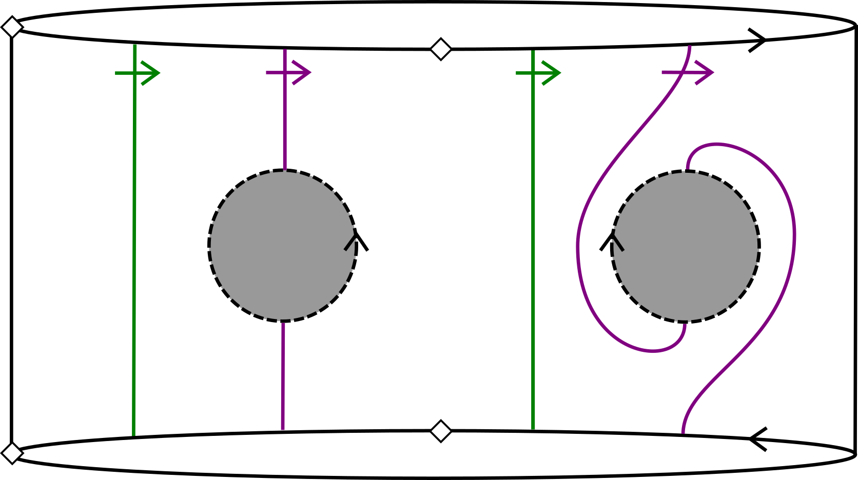
Recall that $B$ denotes a fixed basis for $\mathrm{\mathbf{F}}_{r}$. Following Claim 2.1, we assume that $w_{1}\cdots w_{\ell}\in\left[\mathrm{\mathbf{F}}_{r},\mathrm{\mathbf{F}}_{r}\right]$, namely, that for every letter $x\in B$, the total number of instances of $x^{+1}$ in $w_{1},\ldots,w_{\ell}$ is equal to that of $x^{-1}$, and we denote this number by $L_{x}\in\mathbb{Z}_{\geq 0}$. In particular, $\left|w_{1}\right|+\ldots+\left|w_{\ell}\right|=2\sum_{x\in B}L_{x}$. We also denote by $\mathrm{MATCH}_{x}\left(w_{1},\ldots,w_{\ell}\right)$ the set of bijections from the instances of $x^{+1}$ to the instances of $x^{-1}$, so that $\left|\mathrm{MATCH}_{x}\left(w_{1},\ldots,w_{\ell}\right)\right|=L_{x}!$.

Let $\kappa=\left\{\kappa_{x}\right\}_{x\in B}\in\left(\mathbb{Z}_{\geq 0}\right)^{B}$ be an assignment of a non-negative integer to every basis element. We denote by $\mathrm{MATCH}^{\kappa}\left(w_{1},\ldots,w_{\ell}\right)$ the Cartesian product of sets of matchings, with $\kappa_{x}+1$ copies of $\mathrm{MATCH}_{x}\left(w_{1},\ldots,w_{\ell}\right)$ for every $x\in B$, namely,

$$\mathrm{MATCH}^{\kappa}\left(w_{1},\ldots,w_{\ell}\right)\stackrel{{\scriptstyle\mathrm{def}}}{{=}}\prod_{x\in B}\mathrm{MATCH}_{x}\left(w_{1},\ldots,w_{\ell}\right)^{\kappa_{x}+1}.$$

The following definition presents the construction of a surface from an element of $\mathrm{MATCH}^{\kappa}\left(w_{1},\ldots,w_{\ell}\right)$. We use the notation $\left[k\right]\stackrel{{\scriptstyle\mathrm{def}}}{{=}}\left\{0,1,\ldots,k\right\}$ for a non-negative integer $k$.

Definition 2.7.

Let $w_{1},\ldots,w_{\ell}\in\mathrm{\mathbf{F}}_{r}\setminus\left\{1\right\}$ be a balanced set of words, let $\kappa\in\left(\mathbb{Z}_{\geq 0}\right)^{B}$ and let $\sigma\in\mathrm{MATCH}^{\kappa}\left(w_{1},\ldots,w_{\ell}\right)$ be a tuple of matchings. We denote by $\sigma_{x,0},\ldots,\sigma_{x,\kappa_{x}}$ the $\kappa_{x}+1$ matchings from $\mathrm{MATCH}_{x}\left(w_{1},\ldots,w_{\ell}\right)$ in $\sigma$. From this data we construct a surface $\Sigma_{\sigma}$ as a CW-complex as follows:

• For $1\neq w\in\mathrm{\mathbf{F}}_{r}$ define $S^{1}\left(w\right)$ to be an oriented $1$-sphere $S^{1}$ with additional marked points as follows: there are $\left|w\right|$ points marked $o$, which we call $o$-points. These points cut the $1$-sphere into $\left|w\right|$ intervals, which are in bijection with the letters of $w$, in the suitable cyclic order. For every letter of $w$, if the letter is $x^{\pm 1}$, we mark additional $\kappa_{x}+1$ points on the interval corresponding to that letter. These marked points are labeled $\left(x,0\right),\ldots,\left(x,\kappa_{x}\right)$ and are ordered according to the orientation of $S^{1}\left(w\right)$ if the letter is $x^{+1}$, or in reverse orientation if the letter is $x^{-1}$. We call a point labeled $\left(x,j\right)$ for some $x\in B$ and $j\in\left[\kappa_{x}\right]$ an $\left(x,j\right)$-point or a $z$-point if the exact $x$ and $j$ do not matter.

• The one-dimensional skeleton of $\Sigma_{\sigma}$ consists of $S^{1}\left(w_{1}\right),\ldots,S^{1}\left(w_{\ell}\right)$, together with additional $\sum_{x\in B}L_{x}\left(\kappa_{x}+1\right)$ edges (1-cells), referred to as matching-edges: for every $x\in B$ and $j\in\left[\kappa_{x}\right]$, introduce $L_{x}$ edges describing the matching $\sigma_{x,j}$. Namely, for every $x^{+1}$-letter $\lambda$ of $w_{1},\ldots,w_{\ell}$, introduce an edge between the $\left(x,j\right)$-point on the interval corresponding to $\lambda$ and the $\left(x,j\right)$-point on the interval corresponding to the $x^{-1}$-letter $\sigma_{x,j}\left(\lambda\right)$. This is illustrated in the left part of Figure 2.1.

• Finally, $2$-cells are attached as follows: consider cycles in the $1$-skeleton which are obtained by starting at some marked point in $S^{1}\left(w_{i}\right)$ for some $i=1,\ldots,\ell$, moving orientably along $S^{1}\left(w_{i}\right)$ until the next $z$-point, then following the matching-edge emanating from this $z$-point and arriving at some $z$-point in $S^{1}\left(w_{i^{\prime}}\right)$ for some $i^{\prime}$, then moving orientably along $S^{1}\left(w_{i^{\prime}}\right)$ until the next $z$-point, continuing along the matching-edge and so on until a cycle has been completed. A 2-cell (a disc) is glued along every such cycle.

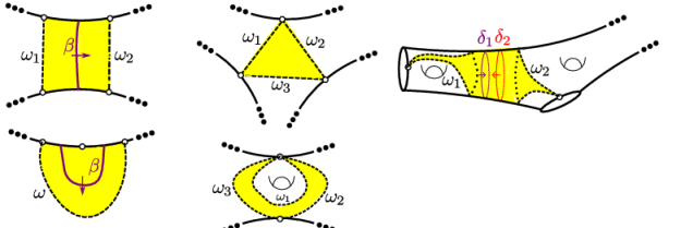
• From the construction of $\Sigma_{\sigma}$, it is clear it is a surface, with boundary $S^{1}\left(w_{1}\right)\sqcup\ldots\sqcup S^{1}\left(w_{\ell}\right)$ and with orientation prescribed from the boundary. Moreover, every $2$-cell $D$ belongs to exactly one of the following categories:

  • Either there is an $o$-point at every component of $\partial D\cap\partial\Sigma_{\sigma}$, in which case we call $D$ an $o$-disc,

  • or, $\partial D$ contains no $o$-points, in which case we call $D$ a $z$-disc. In this case, there are some $x\in B$ with $\kappa_{x}\geq 1$ and $j\in\left[\kappa_{x}-1\right]$ such that the marked points in $\partial D$ are exactly of two types: $\left(x,j\right)$-points and $\left(x,j+1\right)$-points. In this case we call the $z$-disc $D$ also an $\left(x,j\right)$-disc. See Figure 2.1.

• Let $\chi\left(\sigma\right)$ denote the Euler characteristic of this surface, namely $\chi\left(\sigma\right)\stackrel{{\scriptstyle\mathrm{def}}}{{=}}\chi\left(\Sigma_{\sigma}\right)$.

?figurename? 2.1: On the left is the 1-skeleton of $\Sigma_{\sigma}$ for $w=\left[x,y\right]\left[x,z\right]=x_{1}y_{2}X_{3}Y_{4}x_{5}z_{6}X_{7}Z_{8}$, with $\kappa_{x}=\kappa_{y}=1$ and $\kappa_{z}=0$ and with the matchings $\sigma_{x,0}=\left(x_{1}\mapsto X_{3};\leavevmode\nobreak\ x_{5}\mapsto X_{7}\right)$, $\sigma_{x,1}=\left(x_{1}\mapsto X_{7};\leavevmode\nobreak\ x_{5}\mapsto X_{3}\right)$, $\sigma_{y,0}=\sigma_{y,1}=\left(y_{2}\mapsto Y_{4}\right)$ and $\sigma_{z,0}=\left(z_{6}\mapsto Z_{8}\right)$. Dashed lines are matching-edges. The dotted lines trace the boundaries of the two $o$-discs to be glued in (see Definition 2.7). Two additional discs, a $\left(x,0\right)$-disc and a $\left(y,0\right)$-disc are glued along the other types of cycles one can follow (unmarked). The eight $o$-points are marked by $V_{1}$ and black circles. The resulting surface $\Sigma_{\sigma}$ is on the right and is a genus-$2$ surface with one boundary component. In this case, $\chi\left(\sigma\right)=\chi\left(\Sigma_{\sigma}\right)=-3$.

2.3 A formula for ${\cal T}r_{w_{1},\ldots,w_{\ell}}\left(n\right)$ as a rational expression

Our first formula for ${\cal T}r_{w_{1},\ldots,w_{\ell}}\left(n\right)$ is a finite sum over pairs of matchings for every letters, namely over elements in $\mathrm{MATCH}^{\kappa}\left(w_{1},\ldots,w_{\ell}\right)$ with $\kappa_{x}=1$ for every $x\in B$. We denote this $\kappa$ by $\kappa\equiv 1$. In particular, this formula proves Proposition 1.1.

Theorem 2.8 (${\cal T}r_{w_{1},\ldots,w_{\ell}}\left(n\right)$ as finite sum).

Let $w_{1},\ldots,w_{\ell}\in\mathrm{\mathbf{F}}_{r}$ be a balanced set of words.

1. If $n\geq L_{x}$ for every $x\in B$, then

   $${\cal T}r_{w_{1},\ldots,w_{\ell}}\left(n\right)=\sum_{\sigma\in\mathrm{MATCH}^{\kappa\equiv 1}}\left(\prod_{x\in B}\mathrm{Wg}_{L_{x}}\left(\sigma_{x,0}^{-1}\sigma_{x,1}\right)\right)\cdot n^{\#\left\{o\mathrm{-discs\leavevmode\nobreak\ in\leavevmode\nobreak\ }\Sigma_{\sigma}\right\}}$$ (2.6)

   (here $\sigma_{x,0}^{-1}\sigma_{x,1}$ is a permutation of the $x^{+1}$-letters of $w_{1},\ldots,w_{\ell}$).

2. For $n\geq\max_{x\in B}L_{x}$, the function ${\cal T}r_{w_{1},\ldots,w_{\ell}}\left(n\right)$ is a computable rational function in $n$.

3. For $\sigma\in\mathrm{MATCH}^{\kappa\equiv 1}\left(w_{1},\ldots,w_{\ell}\right)$, let $\sigma_{0}=\left(\sigma_{x,0}\right)_{x\in B}$ and $\sigma_{1}=\left(\sigma_{x,1}\right)_{x\in B}$ denote two matchings of the “positive” letters of $w_{1},\ldots,w_{\ell}$ to the “negative” ones. Then the summand in (2.6) corresponding to $\sigma$ is

   $$\mathrm{M\ddot{o}b}\left(\sigma_{0}^{-1}\sigma_{1}\right)\cdot n^{\chi\left(\sigma\right)}+O\left(n^{\chi\left(\sigma\right)-2}\right).$$ (2.7)

?proofname? .

Part $2$ follows from (2.6) as every value of the Weingarten function is computable and in $\mathbb{Q}\left(n\right)$. We now prove part $\left(1\right)$, which we do by way of an example. Let $w_{1}=xyx^{-2}y$ and $w_{2}=xy^{-2}$. Then,

$${\cal T}r_{w_{1},w_{2}}\left(n\right)=\mathbb{E}_{\left(A,B\right)\in{\cal U}(n)\times{\cal U}\left(n\right)}\left[\mathrm{tr}\left(ABA^{-2}B\right)\cdot\mathrm{tr}\left(AB^{-2}\right)\right]$$

$$=\mathbb{E}_{\left(A,B\right)\in{\cal U}(n)\times{\cal U}\left(n\right)}\left[\left(\sum_{i,j,k,\ell,m\in\left[n\right]}A_{i,j}\cdot B_{j,k}\cdot A_{\,\,k,\ell}^{-1}\cdot A_{\leavevmode\nobreak\ \ell,m}^{-1}\cdot B_{m,i}\right)\left(\sum_{I,J,K\in\left[n\right]}A_{I,J}\cdot B_{\leavevmode\nobreak\ J,K}^{-1}\cdot B_{\,\,K,I}^{-1}\right)\right]$$

$$=\sum_{i,j,k,\ell,m,I,J,K\in\left[n\right]}\mathbb{E}_{\left(A,B\right)\in{\cal U}(n)\times{\cal U}\left(n\right)}\left[A_{i,j}\cdot B_{j,k}\cdot\overline{A_{\ell,k}}\cdot\overline{A_{m,\ell}}\cdot B_{m,i}\cdot A_{I,J}\cdot\overline{B_{K,J}}\cdot\overline{B_{I,K}}\right]$$

$$=\sum_{i,j,k,\ell,m,I,J,K\in\left[n\right]}\left(\mathbb{E}_{A\in{\cal U}(n)}\left[A_{i,j}\cdot A_{I,J}\cdot\overline{A_{\ell,k}}\cdot\overline{A_{m,\ell}}\right]\right)\cdot\left(\mathbb{E}_{B\in{\cal U}(n)}\left[B_{j,k}\cdot B_{m,i}\cdot\overline{B_{K,J}}\cdot\overline{B_{I,K}}\right]\right).$$ (2.8)

Note that there is a clear correspondence between the $o$-points in $S^{1}\left(w_{1}\right)$ and the indices $i,j,k,\ell,m$ and between the $o$-points in $S^{1}\left(w_{2}\right)$ and the indices $I,J,K$ (see Figure 2.2).

?figurename? 2.2: The 1-skeleton of the surface $\Sigma_{\sigma}$ for the tuple of matchings $\sigma\in\mathrm{MATCH}^{\kappa\equiv 1}\left(xyx^{-2}y,xy^{-2}\right)$ specified in the proof of Theorem 2.8. The $o$-points are identified with the indices $i,j,k,\ell,m$ and $I,J,K$ that appear in the computation of ${\cal T}r_{xyx^{-2}y,xy^{-2}}\left(n\right)$. The $o$-discs of $\Sigma_{\sigma}$ (two of these in the current case) are in one-to-one correspondence with the blocks of indices determined by $\sigma$, and for every $x\in B$, the $\left(x,0\right)$-discs (one for each letter in the current case) are in one-to-one correspondence with the cycles of the permutation $\sigma_{x,0}^{-1}\sigma_{x,1}$.

Now we use Theorem 2.5 to replace each of the two integrals inside the sum by a summation over pairs of matchings. For the first integral we go over all bijections $\left\{i,I\right\}\overset{\sim}{\to}\left\{\ell,m\right\}$ and $\left\{j,J\right\}\overset{\sim}{\to}\left\{k,\ell\right\}$, and we think of them as elements $\sigma_{x,0},\sigma_{x,1}\in\mathrm{MATCH}_{x}\left(w_{1},w_{2}\right)$ by thinking of a matching between two $z$-points as a matching of the adjacent $o$-points. For example, the $\left(x,0\right)$-point in the first letter of $w_{1}$ is adjacent to the $o$-point $i$, and the $\left(x,1\right)$-point in the same letter is adjacent to the $o$-point $j$. Similarly, we go over all bijections $\sigma_{y,0}$ and $\sigma_{y,1}$ for the second integral. Changing the order of summation, we sum first over $\sigma_{x,0}$, $\sigma_{x,1}$, $\sigma_{y,0}$ and $\sigma_{y,1}$, and only then over the indices $i,j,\ldots,K$. This turns (2.8) into a sum over $\mathrm{MATCH}^{\kappa\equiv 1}\left(w_{1},w_{2}\right)$.

For every set of $\sigma\in\mathrm{MATCH}^{\kappa\equiv 1}\left(w_{1},w_{2}\right)$, we only need to count the number of evaluations of $i,j,\ldots,L$ which “agree” with the permutations. For example, consider the case where

$$\begin{gathered}\underline{\sigma_{x,0}}\\ i\mapsto m\\ I\mapsto\ell\end{gathered}\,\,\,\,\begin{gathered}\underline{\sigma_{x,1}}\\ j\mapsto k\\ J\mapsto\ell\end{gathered}\,\,\,\,\begin{gathered}\underline{\sigma_{y,0}}\\ j\mapsto K\\ m\mapsto I\end{gathered}\,\,\,\,\begin{gathered}\underline{\sigma_{y,1}}\\ k\mapsto K\\ i\mapsto J\end{gathered}$$ (2.9)

(these are the matchings described in Figure 2.2). Note that in this case, both the permutation $\sigma_{x,0}^{-1}\sigma_{x,1}$ and the permutation $\sigma_{y,0}^{-1}\sigma_{y,1}$ are a $2$-cycle. Hence, by Theorem 2.5, the summand corresponding to these matchings is

$${\cal\mathrm{Wg}}_{2}\left(\left(1\leavevmode\nobreak\ 2\right)\right)\cdot{\cal\mathrm{Wg}}_{2}\left(\left(1\leavevmode\nobreak\ 2\right)\right)\cdot\sum_{i,j,k,\ell,m,I,J,K\in\left[n\right]}\delta_{im}\delta_{I\ell}\delta_{jk}\delta_{J\ell}\delta_{jK}\delta_{mI}\delta_{kK}\delta_{iJ},$$

and the product inside the last sum is 1 (and not 0) if and only if $i=m=I=\ell=J$ and $j=k=K$. Here, two indices must have the same value if and only if they belong to the same $o$-disc in $\Sigma_{\sigma}$, hence there are exactly $n^{\#o\mathrm{-discs\leavevmode\nobreak\ in\leavevmode\nobreak\ }\Sigma_{\sigma}}$ contributing values of the indices, each contributing 1 to the summation. For $\sigma$ we defined in (2.9) this number is $n^{2}$, and the total contribution of this $\sigma$ is, thus, ${\cal\mathrm{Wg}}_{2}\left(\left(1\leavevmode\nobreak\ 2\right)\right)^{2}\cdot n^{2}=\frac{1}{\left(n^{2}-1\right)^{2}}$. The total summation over all the $16$ elements of $\mathrm{MATCH}^{\kappa\equiv 1}\left(w_{1},w_{2}\right)$ is $\frac{1}{n^{2}-1}$. Since the same argument works for every $w_{1},\ldots,w_{\ell}\in\mathrm{\mathbf{F}}_{r}$, this proves part $\left(1\right)$.

Recall that for $\pi\in S_{L}$, we have $\left\|\pi\right\|=L-\#\mathrm{cycles}\left(\pi\right)$. The number of cycles in the permutation $\sigma_{x,0}^{-1}\sigma_{x,1}\in S_{L_{x}}$ is equal to the number of $\left(x,0\right)$-discs in $\Sigma_{\sigma}$. Hence, by Theorem 2.4(1),

$$\prod_{x\in B}\mathrm{Wg}_{L_{x}}\left(\sigma_{x,0}^{-1}\sigma_{x,1}\right) =\prod_{x\in B}\left[\frac{\mathrm{M\ddot{o}b}\left(\sigma_{x,0}^{-1}\sigma_{x,1}\right)}{n^{L_{x}+\left\|\sigma_{x,0}^{-1}\sigma_{x,1}\right\|}}+O\left(\frac{1}{n^{L_{x}+\left\|\sigma_{x,0}^{-1}\sigma_{x,1}\right\|+2}}\right)\right]$$

$$=\prod_{x\in B}\left[\frac{\mathrm{M\ddot{o}b}\left(\sigma_{x,0}^{-1}\sigma_{x,1}\right)}{n^{2L_{x}-\#\left\{\left(x,0\right)\mathrm{-discs\leavevmode\nobreak\ in\leavevmode\nobreak\ \Sigma_{\sigma}}\right\}}}+O\left(\frac{1}{n^{2L_{x}-\#\left\{\left(x,0\right)\mathrm{-discs\leavevmode\nobreak\ in\leavevmode\nobreak\ \Sigma_{\sigma}}\right\}+2}}\right)\right]$$

$$=\frac{\mathrm{M\ddot{o}b}\left(\sigma_{0}^{-1}\sigma_{1}\right)}{n^{2L-\#\left\{z\mathrm{-discs\leavevmode\nobreak\ in\leavevmode\nobreak\ \Sigma_{\sigma}}\right\}}}+O\left(\frac{1}{n^{2L-\#\left\{z\mathrm{-discs\leavevmode\nobreak\ in\leavevmode\nobreak\ \Sigma_{\sigma}}\right\}-2}}\right),$$

where $L=\sum_{x\in B}L_{x}$ is the total number of positive letters in $w_{1},\ldots,w_{\ell}$. We are done proving part $\left(3\right)$ as

$$\chi\left(\sigma\right)=\chi\left(\Sigma_{\sigma}\right)=-2L+\#\left\{\mathrm{discs\leavevmode\nobreak\ in\leavevmode\nobreak\ \!}\Sigma_{\sigma}\right\}.$$

∎

2.4 A formula for ${\cal T}r_{w_{1},\ldots,w_{\ell}}\left(n\right)$ as Laurent expansion

We now give an alternative formula for ${\cal T}r_{w_{1},\ldots,w_{\ell}}\left(n\right)$, which also uses surfaces constructed from matchings of the letters of $w_{1},\ldots,w_{\ell}$. The sum in (2.6) is finite, it proves the rationality of ${\cal T}r_{w_{1},\ldots,w_{\ell}}\left(n\right)$, and allows a finite algorithm to compute it. The alternative formula we introduce next has the disadvantage that it is an infinite sum (unless $L_{x}\leq 1$ for every $x\in B$). However, it has the advantage of simplifying greatly the contribution of every surface involved in the computation, as well as being an important step towards establishing Theorem 1.7. This formula is derived from (2.6) together the asymptotic expansion of the Weingarten function developed in [Col03] and depicted in Theorem 2.4(2) above.

The formula uses a restricted set of tuples of matchings which, for a given $\kappa\in\left(\mathbb{Z}_{\geq 0}\right)^{B}$, we denote by $\mathrm{\overline{MATCH}}^{\kappa}\left(w_{1},\ldots,w_{\ell}\right)$: this is the subset of $\mathrm{MATCH}^{\kappa}\left(w_{1},\ldots,w_{\ell}\right)$ with the restriction that no two adjacent matchings are identical, namely, that $\sigma_{x,j}\neq\sigma_{x,j+1}$ for every $x\in B$ and $0\leq j\leq\kappa_{x}-1$. We also denote by $\mathrm{\overline{MATCH}}^{*}\left(w_{1},\ldots,w_{\ell}\right)$ the union of restricted sets of matchings over all possible $\kappa$:

$$\mathrm{\overline{MATCH}}^{*}\left(w_{1},\ldots,w_{\ell}\right)\stackrel{{\scriptstyle\mathrm{def}}}{{=}}\coprod_{\kappa\in\left(\mathbb{Z}_{\geq 0}\right)^{B}}\mathrm{\overline{MATCH}}^{\kappa}\left(w_{1},\ldots,w_{\ell}\right),$$

and for $\sigma\in\mathrm{\overline{MATCH}}^{*}\left(w_{1},\ldots,w_{\ell}\right)$ denote by $\kappa\left(\sigma\right)$ and $\kappa_{x}\left(\sigma\right)$ the corresponding values of $\kappa$ and $\kappa_{x}$. Also, for $\kappa\in\left(\mathbb{Z}_{\geq 0}\right)^{B}$ let $\left|\kappa\right|\stackrel{{\scriptstyle\mathrm{def}}}{{=}}\sum_{x\in B}\kappa_{x}$.

Theorem 2.9 (Laurent Combinatorial Formula for ${\cal T}r_{w_{1},\ldots,w_{\ell}}\left(n\right)$).

Let $w_{1},\ldots,w_{\ell}\in\mathrm{\mathbf{F}}_{r}$ be a balanced set of words. If $n\geq L_{x}$ for every $x\in B$, then

$${\cal T}r_{w_{1},\ldots,w_{\ell}}\left(n\right)=\sum_{\sigma\in\mathrm{\overline{MATCH}}^{*}\left(w_{1},\ldots,w_{\ell}\right)}\left(-1\right)^{\left|\kappa\left(\sigma\right)\right|}n^{\chi\left(\sigma\right)}.$$ (2.10)

?proofname?.

This proof relies on grouping the summands in (2.10) according to the “extreme” bijections $\left\{\sigma_{x,0},\sigma_{x,\kappa_{x}}\right\}_{x\in B}$ and show that the total contribution of the summands with extreme bijections $\tau=\left\{\tau_{x,0},\tau_{x,1}\right\}_{x}\in\mathrm{MATCH}^{\kappa\equiv 1}\left(w_{1},\ldots,w_{\ell}\right)$ is equal to $\left(\prod_{x\in B}\mathrm{Wg}_{L_{x}}\left(\tau_{x,0}^{-1}\circ\tau_{x,1}\right)\right)\cdot n^{\#\left\{o\mathrm{-discs\leavevmode\nobreak\ in\leavevmode\nobreak\ }\Sigma_{\tau}\right\}}$. This is enough by Theorem 2.8.

In (2.3) above, substitute $\theta_{i}=\rho_{1}\cdots\rho_{i}$ to obtain

$${\cal\mathrm{Wg}}_{L}\left(\pi\right)=\frac{1}{n^{L}}\sum_{k\in\mathbb{Z}_{\geq 0}}\sum_{\mathrm{id}=\theta_{0}\neq\theta_{1}\neq\ldots\neq\theta_{k-1}\neq\theta_{k}=\pi}\frac{\left(-1\right)^{k}}{n^{\left\|\theta_{0}^{-1}\theta{}_{1}\right\|+\left\|\theta_{1}^{-1}\theta_{2}\right\|+\ldots+\left\|\theta_{k-1}^{-1}\theta_{k}\right\|}}.$$

Substituting $L=L_{x}$ and $\pi=\tau_{x,0}^{-1}\cdot\tau_{x,1}$, we get

$${\cal\mathrm{Wg}}_{L_{x}}\left(\tau_{x,0}^{-1}\cdot\tau_{x,1}\right)=\frac{1}{n^{L_{x}}}\sum_{k\in\mathbb{Z}_{\geq 0}}\sum_{\begin{gathered}{\scriptstyle\theta_{0},\ldots,\theta_{k}\in\mathrm{Sym}\left(x^{+1}\mathrm{-letters\leavevmode\nobreak\ of}\leavevmode\nobreak\ w_{1},\ldots,w_{\ell}\right)}\\ {\scriptstyle\mathrm{s.t.\leavevmode\nobreak\ }\mathrm{id}=\theta_{0}\neq\theta_{1}\neq\ldots\neq\theta_{k-1}\neq\theta_{k}=\tau_{x,0}^{-1}\tau_{x,1}}\end{gathered}}\frac{\left(-1\right)^{k}}{n^{\left\|\theta_{0}^{-1}\theta{}_{1}\right\|+\left\|\theta_{1}^{-1}\theta_{2}\right\|+\ldots+\left\|\theta_{k-1}^{-1}\theta_{k}\right\|}}.$$

Multiplying all permutations from the left by $\tau_{x,0}$ and substituting $\sigma_{i}=\tau_{x,0}\theta_{i}$, one obtains:

$${\cal\mathrm{Wg}}_{L_{x}}\left(\tau_{x,0}^{-1}\cdot\tau_{x,1}\right)=\frac{1}{n^{L_{x}}}\sum_{k\in\mathbb{Z}_{\geq 0}}\sum_{\begin{gathered}{\scriptstyle\sigma_{0},\ldots,\sigma_{k}\in\mathrm{MATCH}_{x}\left(w_{1},\ldots,w_{\ell}\right)}\\ {\scriptstyle\mathrm{s.t.\leavevmode\nobreak\ }\tau_{x,0}=\sigma_{0}\neq\sigma_{1}\neq\ldots\neq\sigma_{k-1}\neq\sigma_{k}=\tau_{x,1}}\end{gathered}}\frac{\left(-1\right)^{k}}{n^{\left\|\sigma_{0}^{-1}\sigma{}_{1}\right\|+\left\|\sigma_{1}^{-1}\sigma_{2}\right\|+\ldots+\left\|\sigma_{k-1}^{-1}\sigma_{k}\right\|}}.$$ (2.11)

Note that, by construction, the number of $o$-discs in $\Sigma_{\sigma}$ depends solely on the extreme bijections in $\sigma$, namely on $\left\{\sigma_{x,0},\sigma_{x,\kappa_{x}}\right\}_{x\in B}$. Thus, together with (2.6) we obtain

$${\cal T}r_{w_{1},\ldots,w_{\ell}}\left(n\right)=\sum_{\tau\in\mathrm{MATCH}^{\kappa\equiv 1}\left(w_{1},\ldots,w_{\ell}\right)}\left(\prod_{x\in B}\mathrm{Wg}_{L_{x}}\left(\tau_{x,0}^{-1}\circ\tau_{x,1}\right)\right)\cdot n^{\#\left\{o\mathrm{-discs\leavevmode\nobreak\ in\leavevmode\nobreak\ }\Sigma_{\tau}\right\}}$$

$$=\sum_{\tau\in\mathrm{MATCH}^{\kappa\equiv 1}}\frac{n^{\#\left\{o\mathrm{-discs\leavevmode\nobreak\ in}\leavevmode\nobreak\ \Sigma_{\tau}\right\}}}{n^{\sum_{x}L_{x}}}\sum_{\kappa\in\left(\mathbb{Z}_{\geq 0}\right)^{B}}\sum_{\begin{gathered}{\scriptstyle\sigma\in\mathrm{\overline{MATCH}}^{\kappa}}\leavevmode\nobreak\ s.t.\\ {\scriptstyle\sigma_{x,0}=\tau_{x,0}\leavevmode\nobreak\ \&\leavevmode\nobreak\ \sigma_{x,\kappa_{x}}=\tau_{x,1}}\end{gathered}}\frac{\left(-1\right)^{\left|\kappa\right|}}{n^{\sum_{x}\sum_{j=0}^{\kappa_{x}-1}\left\|\sigma_{x,j}^{-1}\cdot\sigma_{x,j+1}\right\|}}$$

$$=\sum_{{\scriptscriptstyle\sigma\in\mathrm{\overline{MATCH}}^{*}\left(w_{1},\ldots,w_{\ell}\right)}}\left(-1\right)^{\left|\kappa\left(\sigma\right)\right|}n^{\#\left\{o\mathrm{-discs\leavevmode\nobreak\ in}\leavevmode\nobreak\ \Sigma_{\sigma}\right\}-\sum_{x}\left(L_{x}+\sum_{j=0}^{\kappa_{x}\left(\sigma\right)-1}\left\|\sigma_{x,j}^{-1}\cdot\sigma_{x,j+1}\right\|\right)}.$$

It is thus enough to explain why

$$\chi\left(\sigma\right)=\#\left\{o\mathrm{-discs\leavevmode\nobreak\ in}\leavevmode\nobreak\ \Sigma_{\sigma}\right\}-\sum_{x}\left(L_{x}+\sum_{j=0}^{\kappa_{x}\left(\sigma\right)-1}\left\|\sigma_{x,j}^{-1}\cdot\sigma_{x,j+1}\right\|\right).$$

• The number of vertices in $\Sigma_{\sigma}$ is $\sum_{x\in B}\left(2\kappa_{x}\left(\sigma\right)+4\right)L_{x}$ (consisting of $\kappa_{x}\left(\sigma\right)+1$ $z$-points and a single $o$-point for each of the $2L_{x}$ $x^{\pm 1}$-letters in $w_{1},\ldots,w_{\ell}$).

• The number of $1$-cells in $\Sigma_{\sigma}$ is $\Sigma_{x\in B}\left(3\kappa_{x}\left(\sigma\right)+5\right)L_{x}$ (there are $\sum_{x\in B}\left(2\kappa_{x}\left(\sigma\right)+4\right)L_{x}$ $1$-cells along the boundary components, and additional $\sum_{x\in B}\left(\kappa_{x}\left(\sigma\right)+1\right)L_{x}$ bijection-edges).

• Finally, it is easy to see from Definition 2.7 that the number of cycles in the permutation $\sigma_{x,j}^{-1}\cdot\sigma_{x,j+1}$ is identical to the number of $\left(x,j\right)$-discs in $\Sigma_{\sigma}$, so that

  $$\left\|\sigma_{x,j}^{-1}\cdot\sigma_{x,j+1}\right\|=L_{x}-\#\left\{\left(x,j\right)\mathrm{-discs\leavevmode\nobreak\ in}\leavevmode\nobreak\ \Sigma_{\sigma}\right\}.$$

Therefore,

$$\chi\left(\sigma\right) = \left[\sum_{x\in B}\left(2\kappa_{x}\left(\sigma\right)+4\right)L_{x}\right]-\left[\sum_{x\in B}\left(3\kappa_{x}\left(\sigma\right)+5\right)L_{x}\right]+$$ (2.12)

$$+\left[\sum_{x\in B}\sum_{j=0}^{\kappa_{x}\left(\sigma\right)-1}\#\left\{\left(x,j\right)\mathrm{-discs\leavevmode\nobreak\ in}\leavevmode\nobreak\ \Sigma_{\sigma}\right\}\right]+\#\left\{o\mathrm{-discs\leavevmode\nobreak\ in}\leavevmode\nobreak\ \Sigma_{\sigma}\right\}$$

$$= \#\left\{o\mathrm{-discs\leavevmode\nobreak\ in}\leavevmode\nobreak\ \Sigma_{\sigma}\right\}+\sum_{x\in B}\left[\left(-\kappa_{x}\left(\sigma\right)-1\right)L_{x}+\sum_{j=0}^{\kappa_{x}\left(\sigma\right)-1}\left(L_{x}-\left\|\sigma_{x,j}^{-1}\cdot\sigma_{x,j+1}\right\|\right)\right]$$

$$= \#\left\{o\mathrm{-discs\leavevmode\nobreak\ in}\leavevmode\nobreak\ \Sigma_{\tilde{\sigma}}\right\}-\sum_{x\in B}\left[L_{x}+\sum_{j=0}^{\kappa_{x}\left(\sigma\right)-1}\left\|\sigma_{x,j}^{-1}\cdot\sigma_{x,j+1}\right\|\right].$$

∎

It is implicit in Theorem 2.9 and its proof that there are only finitely many sets of sequences of bijections $\sigma$ with contribution of a given order. Namely, for every integer $\chi_{0}$ there are finitely many $\sigma$ in the summation (2.10) with $\chi\left(\sigma\right)=\chi_{0}$. This is true because the same property holds for the asymptotic expansion of the Weingarten function in (2.3). However, for completeness, we give a direct proof for this fact:

Claim 2.10.

For every $\chi_{0}\in\mathbb{Z}$ there are finitely many sets $\sigma$ in the sum (2.10) with $\chi\left(\sigma\right)=\chi_{0}$.

?proofname?.

The number of $o$-discs in $\Sigma_{\sigma}$ is bounded by the number of $o$-points in $S^{1}\left(w_{1}\right)\cup\ldots\cup S^{1}\left(w_{\ell}\right)$. All sets $\sigma$ in the sum (2.10) satisfy $\sigma_{x,j}\neq\sigma_{x,j+1}$ for all $x\in B$ and $0\leq j\leq\kappa_{x}-1$, and so $\left\|\sigma_{x,j}^{-1}\cdot\sigma_{x,j+1}\right\|\geq 1$. Thus, from (2.12) we obtain that if $\chi\left(\sigma\right)=\chi_{0}$ then

$$\chi_{0}=\chi\left(\sigma\right)\leq\#\left\{o\mathrm{-points\leavevmode\nobreak\ in}\leavevmode\nobreak\ S^{1}\left(w_{1}\right)\cup\ldots\cup S^{1}\left(w_{\ell}\right)\right\}-\sum_{x\in B}\left[L_{x}+\kappa_{x}\left(\sigma\right)\right].$$

Hence

$$\sum_{x\in B}\kappa_{x}\left(\sigma\right)\leq\#\left\{o\mathrm{-points\leavevmode\nobreak\ in}\leavevmode\nobreak\ S^{1}\left(w_{1}\right)\cup\ldots\cup S^{1}\left(w_{\ell}\right)\right\}-\chi_{0}-\sum_{x\in B}L_{x}.$$

Since the right hand side is independent of $\sigma$, the proof is completed. ∎

The duality between the two types of formulas in Theorems 2.8 and 2.9 will be manifested also in the next section. Our main object of study will be the complex ${\cal T}\left(\Sigma,f\right)$ of transverse maps which, similarly to the sets in the infinite formula (2.10), consists of sequences of arcs and curves of arbitrary lengths, but with the single constraint that two consecutive objects in every sequence must be different from each other (strict transverse maps – see Definition 3.3). However, for one of the main results about ${\cal T}\left(\Sigma,f\right)$, namely, its being contractible, we return to the model of sequences of length two without the constraint of two consecutive objects being different – see Definition 3.15.

2.5 Maps from the surfaces to the bouquet

In Definition 2.7 and in Theorems 2.8 and 2.9 we introduced surfaces associated with $w_{1},\ldots,w_{\ell}$ and tuples of matchings. The following definition introduces a natural map from these surfaces to the bouquet so that each surface and its associated map turns into an admissible pair for $w_{1},\ldots,w_{\ell}$.

Definition 2.11.

Let $w_{1},\ldots,w_{\ell}\in\mathrm{\mathbf{F}}_{r}$, let $\sigma\in\mathrm{MATCH}^{\kappa}\left(w_{1},\ldots,w_{\ell}\right)$ for some $\kappa\in\left(\mathbb{Z}_{\geq 0}\right)^{B}$ and let $\Sigma_{\sigma}$ be the surface constructed in Definition 2.7. Define $f_{\sigma}\colon\Sigma_{\sigma}\to{\textstyle\bigvee^{r}S^{1}}$ as follows:

• For every $x\in B$, mark $\kappa_{x}+1$ distinct points on the circle of the bouquet ${\textstyle\bigvee^{r}S^{1}}$ corresponding to $x$, away from the wedge point $o$, and label them $\left(x,0\right),\ldots,\left(x,\kappa_{x}\right)$ in the order of the orientation of the circle. See Figure 2.3.

• The preimage through $f_{\sigma}^{-1}$ of $\left(x,j\right)\in{\textstyle\bigvee^{r}S^{1}}$ is exactly the bijection-edges corresponding to $\sigma_{x,j}$, which contain the $\left(x,j\right)$-points of $\Sigma_{\sigma}$ as their endpoints.

• The $o$-points in $\Sigma_{\sigma}$ are mapped to $o\in{\textstyle\bigvee^{r}S^{1}}$.

• On $S^{1}\left(w_{i}\right)$, on each of the $\left|w\right|$ intervals, if the interval $I$ corresponds to the letter $x^{\varepsilon}$, $\varepsilon\in\left\{\pm 1\right\}$, $f_{\sigma}\Big{|}_{I}$ traces the $x$-circle in ${\textstyle\bigvee^{r}S^{1}}$ monotonically, with orientation prescribed by $\varepsilon$.

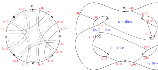
• Finally, for every open disc $D$ in the CW-complex $\Sigma_{\sigma}$, the image of $f_{\sigma}$ along $\partial D$ is nullhomotopic, so there is a unique way to extend it to $D$, up to homotopy, and we extend it so that the image of $f$ on the interior of $D$ avoids the marked points $\left\{\left(x,j\right)\right\}_{x\in B,j\in\left[\kappa_{x}\right]}\subset{\textstyle\bigvee^{r}S^{1}}$.

?figurename? 2.3: The wedge ${\textstyle\bigvee^{r}S^{1}}$ with transversion points. Here $r=2$, $B=\left\{x,y\right\}$, $\kappa_{x}=2$ and $\kappa_{y}=3$.

It is evident that $\left(\Sigma_{\sigma},f_{\sigma}\right)$ is admissible for $w_{1},\ldots,w_{\ell}$ (with the appropriate $o$-point in $S^{1}\left(w_{i}\right)$ labeled also as $v_{i}$, for every $i=1,\ldots,\ell$). In particular,

Corollary 2.12.

If $w_{1}\cdots w_{\ell}\in\left[\mathrm{\mathbf{F}}_{r},\mathrm{\mathbf{F}}_{r}\right]$ then $\mathsf{Surfaces}\left(w_{1},\ldots,w_{\ell}\right)\neq\emptyset$.

Another important observation is that every incompressible pair $\left[\left(\Sigma,f\right)\right]\in\mathsf{Surfaces}\left(w_{1},\ldots,w_{\ell}\right)$ has a representative in the form of $\left(\Sigma_{\sigma},f_{\sigma}\right)$ with only one matching per letter:

Proposition 2.13.

Denote by $\mathrm{MATCH}^{\kappa\equiv 0}\left(w_{1},\ldots,w_{\ell}\right)$ the set of matchings corresponding to $\kappa_{x}=0$ for every $x\in B$. Every incompressible pair $\left(\Sigma,f\right)$ which is admissible for $w_{1},\ldots,w_{\ell}$ is equivalent to $\left(\Sigma_{\sigma},f_{\sigma}\right)$ for some $\sigma\in\mathrm{MATCH}^{\kappa\equiv 0}\left(w_{1},\ldots,w_{\ell}\right)$.

?proofname?.

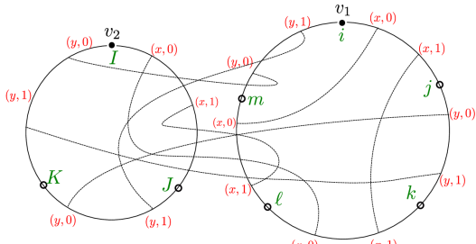
The argument here imitates the one in [Cul81, Theorem 1.4]. Assume $\left(\Sigma,f\right)$ is incompressible. Mark a point $\left(x,0\right)$ on the middle of the circle corresponding to $x$ in ${\textstyle\bigvee^{r}S^{1}}$, and perturb $f$ (relative to the points $v_{1},\ldots,v_{\ell}\in\Sigma$) so that $f\left(\partial_{i}\Sigma\right)$ is monotone, namely, never backtracking, for $i=1,\ldots,\ell$, and so that it becomes transverse to $\left\{\left(x,0\right)\right\}_{x\in B}\subset{\textstyle\bigvee^{r}S^{1}}$ (see Definition 3.1 below). As $f$ is transverse to $\left(x,0\right)\in{\textstyle\bigvee^{r}S^{1}}$, the preimage of $\left(x,0\right)$ consists of a collection of disjoint arcs and curves (in this paper we use the notion “curve” as synonym for “simple closed curve”). Because $f\left(\partial_{i}\Sigma\right)$ is monotone, there are exactly $L_{x}$ arcs, which determine an element $\sigma\in\mathrm{MATCH}^{\kappa\equiv 0}\left(w_{1},\ldots,w_{\ell}\right)$. There are no curves in $f^{-1}\left(\left(x,0\right)\right)$ because such curves would be null-curves, which is impossible with $f$ being incompressible. Finally, $f$ being incompressible also guarantees that the collection of arcs $\coprod_{x\in B}f^{-1}\left(\left(x,0\right)\right)$ cuts $\Sigma$ into discs. Thus $\left(\Sigma,f\right)\sim\left(\Sigma_{\sigma},f_{\sigma}\right)$. ∎

Since the set $\mathrm{MATCH}^{\kappa\equiv 0}\left(w_{1},\ldots,w_{\ell}\right)$ is finite, we obtain:

Corollary 2.14.

There are finitely many classes of incompressible $\left(\Sigma,f\right)$ in $\mathsf{Surfaces}\left(w_{1},\ldots,w_{\ell}\right)$.

In Section 5.2 we address the issue of how one can distinguish the different incompressible classes in $\mathsf{Surfaces}\left(w_{1},\ldots,w_{\ell}\right)$.

At this point we can also derive the asymptotic bounds we have for ${\cal T}r_{w_{1},\ldots,w_{\ell}}\left(n\right)$:

Proof of Corollary 1.8.

Recall that we need to prove that ${\cal T}r_{w_{1},\ldots,w_{\ell}}\left(n\right)=O\left(n^{\chi_{\max}\left(w_{1},\ldots,w_{\ell}\right)}\right)$ where $\chi_{\max}\left(w_{1},\ldots,w_{\ell}\right)$ is the maximal Euler characteristic of a surface in $\mathsf{Surfaces}\left(w_{1},\ldots,w_{\ell}\right)$. Theorem 2.8 says that ${\cal T}r_{w_{1},\ldots,w_{\ell}}\left(n\right)$ is equal to a sum over $\sigma\in\mathrm{MATCH}^{\kappa\equiv 1}\left(w_{1},\ldots,w_{\ell}\right)$, and the contribution of each $\sigma$ is $c\cdot n^{\chi\left(\sigma\right)}+O\left(n^{\chi\left(\sigma\right)-2}\right)$ where $c\in\mathbb{Z}\setminus\left\{0\right\}$. As $\left(\Sigma_{\sigma},f_{\sigma}\right)\in\mathsf{Surfaces}\left(w_{1},\ldots,w_{\ell}\right)$, then by definition $\chi\left(\sigma\right)\leq\chi_{\max}\left(w_{1},\ldots,w_{\ell}\right)$. ∎

Remark 2.15.

In fact, we get even more: every $\left[\left(\Sigma,f\right)\right]\in\mathsf{Surfaces}\left(w_{1},\ldots,w_{\ell}\right)$ attaining $\chi_{\max}\left(w_{1},\ldots,w_{\ell}\right)$ is incompressible, and therefore, by Proposition 2.13, equivalent to $\left(\Sigma_{\sigma},f_{\sigma}\right)$ for some $\sigma\in\mathrm{MATCH}^{\kappa\equiv 0}\left(w_{1},\ldots,w_{\ell}\right)$. This $\sigma$ takes part in the expression for ${\cal T}r_{w_{1},\ldots,w_{\ell}}\left(n\right)$ in Theorem 2.9 and thus one can expect that ${\cal T}r_{w_{1},\ldots,w_{\ell}}\left(n\right)=\Theta\left(n^{\chi_{\max}\left(w_{1},\ldots,w_{\ell}\right)}\right)$. As some of the examples from Table 1 indicate, the coefficient of $n^{\chi_{\max}\left(w_{1},\ldots,w_{\ell}\right)}$ may vanish, but this only happens if the different non-zero contributions cancel out. (One can get to the same conclusion from the finite formula for ${\cal T}r_{w_{1},\ldots,w_{\ell}}\left(n\right)$ in Theorem 2.8, by duplicating every matching in $\sigma\in\mathrm{MATCH}^{\kappa\equiv 0}$ to obtain $\sigma^{\prime}\in\mathrm{MATCH}^{\kappa\equiv 1}\left(w_{1},\ldots,w_{\ell}\right)$, which then satisfies $\left(\Sigma_{\sigma},f_{\sigma}\right)\sim\left(\Sigma_{\sigma^{\prime}},f_{\sigma^{\prime}}\right)$.)

Reduction of the main theorem

Recall that Theorem 2.9 expresses ${\cal T}r_{w_{1},\ldots,w_{\ell}}\left(n\right)$ as a sum over the (generally infinite) set $\mathrm{\overline{MATCH}}^{*}\left(w_{1},\ldots,w_{\ell}\right)$. To prove our main result, Theorem 1.7, we group together all $\sigma\in\mathrm{\overline{MATCH}}^{*}\left(w_{1},\ldots,w_{\ell}\right)$ for which $\left(\Sigma_{\sigma},f_{\sigma}\right)$ belong to the same equivalence class, and show the total contribution of these values of $\sigma$ to (2.10) is exactly the one specified in Theorem 1.7. Accordingly, for $\left[\left(\Sigma,f\right)\right]\in\mathsf{Surfaces}$ we let $\mathrm{\overline{MATCH}}^{*}\left(w_{1},\ldots,w_{\ell};\Sigma,f\right)$ be the $\sigma$’s yielding elements in the class of $\left(\Sigma,f\right)$ . So, recalling the notation “$\sim$” from Definition 1.3,

$$\mathrm{\overline{MATCH}}^{*}\left(w_{1},\ldots,w_{\ell};\Sigma,f\right)\stackrel{{\scriptstyle\mathrm{def}}}{{=}}\left\{\sigma\in\mathrm{\overline{MATCH}}^{*}\left(w_{1},\ldots,w_{\ell}\right)\,\middle|\,\left(\Sigma_{\sigma},f_{\sigma}\right)\sim\left(\Sigma,f\right)\right\}.$$

From Claim 2.10 it follows that $\mathrm{\overline{MATCH}}^{*}\left(w_{1},\ldots,w_{\ell};\Sigma,f\right)$ is finite for every $\left(\Sigma,f\right)\in\mathsf{Surfaces}\left(w_{1},\ldots,w_{\ell}\right)$. Using Theorem 2.9, Theorems 1.4 and 1.7 now reduce to:

Theorem 2.16.

Let $\left[\left(\Sigma,f\right)\right]\in\mathsf{Surfaces}\left(w_{1},\ldots,w_{\ell}\right)$. Then $\chi^{\left(2\right)}\left(\mathrm{MCG}\left(f\right)\right)$ is well defined and given by

$$\chi^{\left(2\right)}\left(\mathrm{MCG}\left(f\right)\right)=\sum_{\sigma\in\mathrm{\overline{MATCH}}^{*}\left(w_{1},\ldots,w_{\ell};\Sigma,f\right)}\left(-1\right)^{\left|\kappa\left(\sigma\right)\right|}.$$ (2.13)

In particular, if $\left[\left(\Sigma,f\right)\right]\in\mathsf{Surfaces}\left(w_{1},\ldots,w_{\ell}\right)$ cannot be realized by any $\sigma\in\mathrm{\overline{MATCH}}^{*}\left(w_{1},\ldots,w_{\ell}\right)$, then $\chi^{(2)}\left(\mathrm{MCG}\left(f\right)\right)=0$. Since there are only finitely many $\sigma$ with $\Sigma_{\sigma}$ of a given Euler characteristic (Claim 2.10), it follows from Theorem 2.16 that, indeed, for any $\chi_{0}\in\mathbb{Z}$, there are only finitely many classes $\left[\left(\Sigma,f\right)\right]\in\mathsf{Surfaces}\left(w_{1},\ldots,w_{\ell}\right)$ with $\chi\left(\Sigma\right)=\chi_{0}$ and for which $\chi^{\left(2\right)}\left(\mathrm{MCG}\left(f\right)\right)\neq 0$.

In the next two sections we describe the constructions and results that lead to the proof of Theorem 2.16 and of Theorem 1.6 which strengthen the result in the case $\left(\Sigma,f\right)$ is incompressible. We hint that the special property of the incompressible case is that the set $\mathrm{\overline{MATCH}}^{*}\left(w_{1},\ldots,w_{\ell};\Sigma,f\right)$ gives rise to a natural complex with one cell for every element $\sigma\in\mathrm{\overline{MATCH}}^{*}\left(w_{1},\ldots,w_{\ell};\Sigma,f\right)$, so that the Euler characteristic of this complex is exactly the right hand side of (2.13). See Section 4.4 for details.

3 A complex of transverse maps

The key ingredient in the proof of our main results is a complex of transverse maps which we associate with a given pair $\left[\left(\Sigma,f\right)\right]\in\mathsf{Surfaces}\left(w_{1},\ldots,w_{\ell}\right)$. In the current section we define it, study important properties and prove it is contractible. In the next section we study the action of $\mathrm{MCG}\left(f\right)$ on this complex and prove our main results.

3.1 Transverse maps

Recall that in this paper the term “curve” is short for a simple closed curve.

Definition 3.1.

Let $\Sigma$ be orientable. A map $f\colon\Sigma\to{\textstyle\bigvee^{r}S^{1}}$ is said to be transverse to a point $p\in{\textstyle\bigvee^{r}S^{1}}\setminus\left\{o\right\}$ if the preimage of $p$ is a disjoint union of arcs and curves, and if in a small tubular neighborhood $U$ of every curve or arc $\gamma$ in the preimage, the two connected components of $U\setminus\gamma$ are mapped to two different “sides” of $p$.

For example, the map $f_{\sigma}$ from Definition 2.11 is transverse to the points $\left\{\left(x,j\right)\right\}_{x\in B,j\in\left[\kappa_{x}\right]}$ in ${\textstyle\bigvee^{r}S^{1}}$. In this case, the preimage of each of these points contains no curves but rather only arcs. We shall consider here different realizations of the homotopy class $\left[f\right]$ of the same map $f\colon\Sigma\to{\textstyle\bigvee^{r}S^{1}}$, which are transverse to different collections of points in ${\textstyle\bigvee^{r}S^{1}}$.

More formally, let $\Sigma$ be a surface and $f$ a map $f\colon\Sigma\to{\textstyle\bigvee^{r}S^{1}}$ so that $\left[\left(\Sigma,f\right)\right]\in\mathsf{Surfaces}\left(w_{1},\ldots,w_{\ell}\right)$. By definition, $\Sigma$ has $\ell$ marked points: one point, labeled $v_{i}$, in every boundary component $\partial_{i}\Sigma$, for $i=1,\ldots,\ell$, and with $f\left(v_{i}\right)=o$. Note that $w_{1},\ldots,w_{\ell}$ are prescribed from $\Sigma$ and $f$ by $w_{i}=f_{*}\left(\overrightarrow{\partial_{i}\Sigma},v_{i}\right)\in\pi_{1}\left({\textstyle\bigvee^{r}S^{1}},o\right)$. For every $i=1,\ldots,\ell$, we mark additional $\left|w_{i}\right|-1$ points on $\partial_{i}\Sigma$ inside $f^{-1}\left(o\right)$, so that $f$ maps the intervals of $\partial_{i}\Sigma$ cut by these points to the letters of $w_{i}$. We let $V_{o}\subset\Sigma$ denote the set of all marked points in $\Sigma$: a total of $\sum_{i=1}^{\ell}\left|w_{i}\right|$ marked points all at the boundary.

Definition 3.2.

Let $\kappa=\left\{\kappa_{x}\right\}_{x\in B}\in\left(\mathbb{Z}_{\geq 0}\right)^{B}$ be a set of non-negative integers. On the circle corresponding to $x$ in ${\textstyle\bigvee^{r}S^{1}}$ mark $\kappa_{x}+1$ disjoint points, $\left(x,0\right),\ldots,\left(x,\kappa_{x}\right)$, arranged as in Definition 2.11 and Figure 2.3. Let $\left[\left(\Sigma,f\right)\right]\in\mathsf{Surfaces}\left(w_{1},\ldots,w_{\ell}\right)$ and $V_{o}\subset f^{-1}\left(o\right)\subseteq\Sigma$ be as above. A map $g\colon\Sigma\to{\textstyle\bigvee^{r}S^{1}}$ is a transverse map realizing $\left(\Sigma,f\right)$ with parameters $\kappa$, if it is homotopic to $f$ relative to $V_{o}$ and transverse to the points $\left\{\left(x,j\right)\right\}_{x\in B,j\in\left[\kappa_{x}\right]}\subset{\textstyle\bigvee^{r}S^{1}}$. Note that, in particular, $g\left(V_{o}\right)=\left\{o\right\}$.

An arc (curve, respectively) in the preimage of $\left(x,j\right)$ is called an $\left(x,j\right)$-arc ($\left(x,j\right)$-curve). Let $U_{o}$ be the connected component of $o$ in ${\textstyle\bigvee^{r}S^{1}}\setminus\left\{\left(x,j\right)\right\}_{x\in B,j\in\left[\kappa_{x}\right]}$. A connected component of $g^{-1}\left(U_{o}\right)$ is called an $o$-zone. For $0\leq j\leq\kappa_{x}-1$, let $I_{x,j}\subset{\textstyle\bigvee^{r}S^{1}}$ be the interval on the $x$-circle cut out by $\left(x,j\right)$ and $\left(x,j+1\right)$. We call a connected component of $g^{-1}\left(I_{x,j}\right)$ an $\left(x,j\right)$-zone, or, if $x$ and $j$ are not relevant, also a $z$-zone. If all zones defined by $g$ are topological discs, we say that $g$ fills $\Sigma$, or that $g$ is filling.

The isotopy class of the transverse map $g$, denoted $\left[g\right]$, contains all transverse maps with the same parameters $\kappa$ which are homotopic to $g$ relative to $V_{o}$ via a homotopy of transverse maps with the same parameters. We stress that the marked points in ${\textstyle\bigvee^{r}S^{1}}$ are allowed to move inside ${\textstyle\bigvee^{r}S^{1}}\setminus\left\{o\right\}$ along the homotopy as long as they remain disjoint.

Note that every $\left(x,j\right)$-arc/curve has a direction from one side of the arc/curve to the other, induced by the orientation of the circle in ${\textstyle\bigvee^{r}S^{1}}$. Since we do not care about the location of the $\left(x,j\right)$-points in ${\textstyle\bigvee^{r}S^{1}}$, a transverse map $g$ for $\left(\Sigma,f\right)$ can be identified with the collection of disjoint “directed” and colored arcs and curves. The isotopy class of $g$ can then be though of as the isotopy class of this collection of arcs and curves relative to $V_{o}$. We illustrate such a collection in Figure 3.1.

Also note, by the definition above, that the boundary of an $\left(x,j\right)$-zone of $g$ consists of pieces of $\partial\Sigma$, of $\left(x,j\right)$-arcs/curves directed inward and of $\left(x,j+1\right)$-arcs/curves directed outward. In contrast, the boundary of an $o$-zone of $g$ consists of pieces of $\partial\Sigma$, of $\left(x,0\right)$-arcs/curves directed outward and of $\left(x,\kappa_{x}\right)$-arcs/curves directed inward, for various $x\in B$. Finally, every point in $V_{o}$ belongs to some $o$-zone of $g$.

?figurename? 3.1: A collection of arcs corresponding to a transverse map realizing $\left(\Sigma,f\right)$, where $\Sigma$ is a genus 1 surface with 2 boundary components, drawn as an annulus with two discs cut out, with boundaries of those discs identified. Here $r=1$ and there is one generator $x$. Green arcs are $(x,0)$-arcs and purple are $(x,1)$-arcs. The marked points $V_{o}$ are diamonds. There are no curves in this system and it is filling. The words at the boundary are $x^{2},x^{-2}$.

Generally, we want to forbid certain trivial or redundant features of transverse maps, as we elaborate in the following definition:

Definition 3.3.

A transverse map for $\left(\Sigma,f\right)$ is called loose if it satisfies

• Restriction 1. There are no $o$-zones nor $z$-zones that contain no marked point from $V_{o}$ and whose boundary arcs and curves have the same color $(x,j)$ and are all oriented pointing inwards or all oriented outwards. Note this rules out the possibility of a zone that is a disc bounded by a closed curve.

• Restriction 2. No segment of the boundary of $\Sigma$ that contains no marked point can be bounded by the end points of two arcs that are equally-labeled and both directed inwards or both outwards. Note that this is the boundary analog of Restriction 1.

A transverse map for $\left(\Sigma,f\right)$ is called strict if it satisfies, in addition,

• Restriction 3. For every $x\in B$ and $0\leq j\leq\kappa_{x}-1$, the collection of $\left(x,j\right)$-arcs and curves is not isotopic to the collection of $\left(x,j+1\right)$-arcs and curves. In other words, there must be at least one $(x,j)$-zone which is neither a rectangle nor an annulus.

Remark 3.4.

• Note that if $g$ fills $\Sigma$ then there are no curves involved in $g$, but only arcs. This is the case, for example, when $g=f_{\sigma}$ as in Definition 2.11.

• Any transverse map for $\left(\Sigma,f\right)$ satisfying Restriction 2 admits exactly $\kappa_{x}+1$ arcs touching every interval in $\partial\Sigma$ corresponding to the letter $x$, one arc for every $j\in\left[\kappa_{x}\right]$. Consequently, it admits exactly $L_{x}$ arcs labeled $\left(x,j\right)$ for every $x\in B$ and $j\in\left[\kappa_{x}\right]$. In addition, if $O$ is an $o$-zone of such a map then every connected component of $\overline{O}\cap\partial\Sigma$ contains exactly one marked point from $V_{o}$.

• If Restriction 2 holds, then Restriction 1 can only fail at zones bounded by curves.

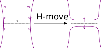
The following local surgery of a transverse map will be very useful in the sequel:

Definition 3.5.

Let $g$ be a transverse map realizing $\left(\Sigma,f\right)$ with parameters $\kappa$. Let $\alpha_{1}$ and $\alpha_{2}$ be each an $\left(x,j\right)$-arc or an $\left(x,j\right)$-curve in the collection corresponding to $g$, where $\alpha_{1}$ and $\alpha_{2}$ have the same color and are not necessarily distinct. Assume further there is an embedded arc-segment $\gamma$ inside the interior of $\Sigma$, with one endpoint in $\alpha_{1}$ and the other in $\alpha_{2}$ such that the interior of $\gamma$ is disjoint from the arc-curve collection of $g$, and such that both $\alpha_{1}$ and $\alpha_{2}$ are directed towards $\gamma$ or both directed away from $\gamma$. We say that the transverse map $g^{\prime}$ realizing $\left(\Sigma,f\right)$ with the same parameters is obtained from $g$ by an H-Move along $\gamma$ if:

• One takes a small collar neighborhood of $\gamma$ to obtain a rectangle whose short sides are contained in $\alpha_{1}$ and in $\alpha_{2}$.

• One deletes the short sides of the rectangle from the arc-curve collection of $g$ and replaces them with the long sides to obtain a new collection which defines $g^{\prime}$. See Figure 3.2.

It is clear that $g^{\prime}$ is homotopic to $g$ as a map but not isotopic as a transverse map.

?figurename? 3.2: The dashed line is the arc-segment $\gamma$ along which the H-move is performed. The two purple segments on the left are parts of $\alpha_{1}$ and $\alpha_{2}$.

3.2 The poset of strict transverse maps

The complex of transverse maps will be defined as the geometric realization of the poset of transverse maps:

Definition 3.6.

Let $\Sigma$ and $f\colon\Sigma\to{\textstyle\bigvee^{r}S^{1}}$ satisfy $\left[\left(\Sigma,f\right)\right]\in\mathsf{Surfaces}\left(w_{1},\ldots,w_{\ell}\right)$. Let $V_{o}\subset f^{-1}\left(o\right)\cap\partial\Sigma$ be defined as above, so $V_{o}\cap\partial_{i}\Sigma$ cuts $\partial_{i}\Sigma$ into $\left|w_{i}\right|$ intervals, each of which is mapped to some $x^{\pm 1}$ with $x\in B$ by $f_{*}$. The poset of transverse maps realizing $\left(\Sigma,f\right)$, denoted ${\cal T}={\cal T}\left(\Sigma,f\right)$ or $\left({\cal T},\preceq\right)$, consists of the set of isotopy classes relative to $V_{o}$ of strict transverse maps realizing $\left(\Sigma,f\right)$. The order is defined by “forgetting points of transversion”. Namely, whenever $g_{1}$ is a transverse map realizing $\left(\Sigma,f\right)$ with parameters $\left\{\kappa_{x}\right\}_{x\in B}$ and $g_{2}$ is identical to $g_{1}$ except we forget a proper (possibly empty) subset of the transversion points $\left\{\left(x,j\right)\right\}_{j\in\left[\kappa_{x}\right]}\subset{\textstyle\bigvee^{r}S^{1}}$ for every $x\in B,$ then the isotopy classes $\left[g_{1}\right]$ and $\left[g_{2}\right]$ satisfy $\left[g_{2}\right]\preceq\left[g_{1}\right]$ in the poset ${\cal T}$.

Of course, the transversion points that remain in $g_{2}$ may need relabeling. Note that we use here strict transverse maps: maps satisfying the three restrictions from Definition 3.3. The role of loose transverse maps will be clarified in the sequel of this section. Another important observation is that if the transverse map $g$ is strict, then so are the maps obtained from $g$ by forgetting transversion points:

Lemma 3.7.

If $g_{1}$ is a strict transverse map realizing $\left(\Sigma,f\right)$ and $g_{2}$ is obtained from $g_{1}$ by forgetting transversion points, then $g_{2}$ is also strict. In other words, if $\left[g_{1}\right]\in{\cal T}$ then $\left[g_{2}\right]\in{\cal T}$.

?proofname?.

It is enough to prove the statement of the lemma in the special case where $g_{2}$ is obtained by forgetting a single point, say the point $\left(x,j\right)$, for some $x\in B$ with $\kappa_{x}\geq 1$ and $j\in\left[\kappa_{x}\right]$. It is obvious that $g_{2}$ satisfies Restriction 3. Let $I\subset\partial_{i}\Sigma\setminus V_{o}$ be an interval cut out by two adjacent marked points. As $g_{1}$ satisfies Restriction 2, all arcs touching $I$ are directed in the same orientation w.r.t. $I$ and this property remains true for $g_{2}$, hence $g_{2}$ satisfies Restriction 2.

As for Restriction 1, assume first that $j=\kappa_{x}$, so every $o$-zone and $\left(x,\kappa_{x}-1\right)$-zone of $g_{1}$ which are neighbors belong to the same $o$-zone of $g_{2}$. Every $z$-zone of $g_{2}$ is also a $z$-zone of $g_{1}$ with the same boundary, so Restriction 1 is not violated there. Let $O\subset\Sigma$ be an $o$-zone of $g_{2}$ that violates Restriction 1. Then $O$ is not an $o$-zone of $g_{1}$, and has to be a union of $o$-zones and $\left(x,\kappa_{x}-1\right)$-zones of $g_{1}$, at least one of each type. In addition, $O$ contains no marked points and has only incoming $\left(x,\kappa_{x}-1\right)$-arcs/curves at its boundary: this is because $g_{1}$ satisfies Restriction 1, every $\left(x,\kappa_{x}-1\right)$-zone has some incoming $\left(x,\kappa_{x}-1\right)$-arc/curve at its boundary, and so $O$ also has some incoming $\left(x,\kappa_{x}-1\right)$-arc/curve at its boundary. But then, every $o$-zone of $g_{1}$ contained in $O$ has no marked points and only incoming $\left(x,\kappa_{x}\right)$-arcs/curves at its boundary, a contradiction.

The proof is analogous if $j=0$ and is similar but even simpler if $1\leq j\leq\kappa_{x}-1$. ∎

Another important observation is that ${\cal T}={\cal T}\left(\Sigma,f\right)$ is not empty.

Lemma 3.8.

Let $\Sigma$, $f$ be as in Definition 3.6, then the poset ${\cal T}={\cal T}\left(\Sigma,f\right)$ is not empty.

?proofname?.

For every $x\in B$, mark a single point $\left(x,0\right)$ in ${\textstyle\bigvee^{r}S^{1}}$ on the circle corresponding to $x$. Perturb $f$ to obtain $g$ that is transverse to the points $\left\{\left(x,0\right)\right\}_{x\in B}$ (without changing the image at $V_{o}$). The resulting map is a transverse map realizing $\left(\Sigma,f\right)$ with parameters $\kappa_{x}=0$ for all $x$. Restriction 3 is automatically satisfied when $\kappa_{x}=0$ for all $x$.

If $g$ violates Restriction 2, then there is a segment $I$ of the boundary cut out by two endpoints of $\left(x,0\right)$-arcs for some $x\in B$, both directed, say, inwards, and without any marked point. Let $\gamma$ be an arc parallel to $I$ slightly away from $\partial\Sigma$ with endpoint at the two arcs cutting $I$. Perform an $H$-move along $\gamma$, and delete the resulting $\left(x,0\right)$-arc parallel to $I$ and $\gamma$. In that manner one can get rid of all violations of Restriction 2.

So assume now that $g$ does not violate Restrictions 2 and 3. Any violation of Restriction 1 is at zones bounded by curves. But any such zone can be simply deleted by removing all its bounding curves. To see that this procedure does not change the homotopy type of the function, note that it can be achieved by a series of H-moves: first perform H-moves along arcs connecting a curve and itself to decrease the genus of the zone to 0. Then, use H-moves between different bounding curves to eventually reduce the number of bounding curves to one. The resulting zone is a disk bounded by a curve which can easily be homotoped away. We can repeat this process until no violations of Restriction 3 remain. The resulting map is a strict transverse map realizing $\left(\Sigma,f\right)$. ∎

3.3 The complex of transverse maps

The complex of transverse maps is defined as a “polysimplicial complex”, meaning that its cells are products of simplices, or polysimplices, as in $\Delta_{k_{1}}\times\Delta_{k_{2}}\times\ldots\times\Delta_{k_{r}}$, where $\Delta_{k}$ is the standard simplex of dimension $k$. Note that the polysimplex $\Delta_{k_{1}}\times\ldots\times\Delta_{k_{r}}$ has dimension $k_{1}+\ldots+k_{r}$.

Definition 3.9.

The complex of transverse maps realizing $\left(\Sigma,f\right)$, denoted $\left|{\cal T}\right|_{\mathrm{poly}}=$ $\left|{\cal T}\left(\Sigma,f\right)\right|_{\mathrm{poly}}$, is a polysimplicial complex with a polysimplex $\mathrm{polysim}\left(\left[g\right]\right)\stackrel{{\scriptstyle\mathrm{def}}}{{=}}\prod_{x}\Delta_{\kappa_{x}}$ for every element $\left[g\right]\in{\cal T}$ with parameters $\left\{\kappa_{x}\right\}_{x\in B}$. The faces of $\mathrm{polysim\left(\left[g\right]\right)}$ are exactly $\left\{\mathrm{polysim}\left(\left[g^{\prime}\right]\right)\,\middle|\,\left[g^{\prime}\right]\preceq\left[g\right]\right\}$. Then $\left|{\cal T}\right|_{\mathrm{poly}}$ is the union of closed cells or disjoint union of open cells:

$$\left|{\cal T}\right|_{\mathrm{poly}}\stackrel{{\scriptstyle\mathrm{def}}}{{=}}\bigcup_{\left[g\right]\in{\cal T}}\overline{\mathrm{polysim}}\left(\left[g\right]\right)=\bigsqcup_{\left[g\right]\in{\cal T}}\mathrm{polysim^{o}\left(\left[g\right]\right).}$$

The topology on $\left|{\cal T}\right|_{\mathrm{poly}}$, as the topology on every (poly-)simplicial complex in this paper, is defined by taking the Euclidean topology on every (poly-)simplex $s$, and by letting a general set $A\subseteq\left|{\cal T}\right|_{\mathrm{poly}}$ to be closed if and only if $A\cap s$ is closed in $s$ for every (poly-)simplex $s$.

We remark that Restriction 3 plays an important role in this definition: it guarantees that different vertices of the closed polysimplex $\overline{\mathrm{polysim}}\left(\left[g\right]\right)$ correspond to different (minimal) elements of ${\cal T}$, hence the closed polysimplices are embedded in $\left|{\cal T}\right|_{\mathrm{poly}}$.

There is an equivalent way to construct the complex of transverse map (up to homeomorphism), as an ordinary simplicial complex: the order complex $\left|{\cal T}\right|$ of ${\cal T}$. This is a standard simplicial complex, with simplices corresponding to chains in ${\cal T}$: every chain $\left[g_{0}\right]\prec\left[g_{1}\right]\prec\ldots\prec\left[g_{m}\right]$ corresponds to an $m$-simplex, with the obvious faces.

Claim 3.10.

$\left|{\cal T}\right|$ is the barycentric subdivision of $\left|{\cal T}\right|_{\mathrm{poly}}$. In particular, $\left|{\cal T}\right|\cong\left|{\cal T}\right|_{\mathrm{poly}}$.

To prove the claim we use the following well-known fact. Here, if $\left(P,\leq_{P}\right)$ and $\left(Q,\leq_{Q}\right)$ are posets, then $\left|P\right|$ is the order complex of $P$, and the direct product $\left(P\times Q,\leq_{P\times Q}\right)$ is defined by $\left(p_{1},q_{1}\right)\leq_{P\times Q}\left(p_{2},q_{2}\right)$ if and only if $p_{1}\leq_{P}p_{2}$ and $q_{1}\leq_{Q}q_{2}$.

Fact 3.11 (e.g. [Wal88, Theorem 3.2]).

Let $P$ and $Q$ be posets. The function $\left|P\times Q\right|\to\left|P\right|\times\left|Q\right|$ defined by

$$\sum\lambda_{i}\left(p_{i},q_{i}\right)\mapsto\left(\sum\lambda_{i}p_{i},\sum\lambda_{i}q_{i}\right)$$

is an homeomorphism.

Proof of Claim 3.10.

Let $\left[g\right]\in{\cal T}$ with parameters $\kappa\in\left(\mathbb{Z}_{\geq 0}\right)^{B}$. We show that the barycentric subdivision of $\overline{\mathrm{polysim}}\left(\left[g\right]\right)$ consists of the simplices corresponding to chains in ${\cal T}$ with top element $\left[g^{\prime}\right]$ satisfying $\left[g^{\prime}\right]\preceq\left[g\right]$. Indeed, this is certainly true in the single-letter case where $r=\left|B\right|=1$ and every polysimplex is merely a simplex. For the general case, let $\left[\gamma^{x}\left(g\right)\right]$ denote the isotopy class of the collection of arcs/curves corresponding to the letter $x$, for $x\in B$. Let $P_{x}\left(g\right)$ denote the poset of all isotopy classes of collections of arcs/curves obtained from $\left[\gamma^{x}\left(g\right)\right]$ by forgetting arcs/curves from a proper subset of the colors $\left[\kappa_{x}\right]$. The single-letter case shows that $\left|P_{x}\left(g\right)\right|\cong\Delta_{\kappa_{x}}$. Since the subposet of ${\cal T}$ given by ${\cal T}_{\preceq\left[g\right]}\stackrel{{\scriptstyle\mathrm{def}}}{{=}}\left\{\left[g^{\prime}\right]\in{\cal T}\,\middle|\,\left[g^{\prime}\right]\preceq\left[g\right]\right\}$ is exactly $\prod_{x\in B}P_{x}\left(g\right)$, Fact 3.11 yields that the order complex of ${\cal T}_{\preceq\left[g\right]}$ is homeomorphic to $\overline{\mathrm{polysim}}\left(\left[g\right]\right)$. ∎

An important property of $\left|{\cal T}\right|_{\mathrm{poly}}$ is that it is finite-dimensional. This is an analog of Claim 2.10 and here, again, Restriction 3 plays an important role:

Lemma 3.12.

The complex $\left|{\cal T}\right|_{\mathrm{poly}}$ is finite dimensional with $\dim\left(\left|{\cal T}\right|_{\mathrm{poly}}\right)\leq\frac{\ell}{2}-\chi\left(\Sigma\right)$.

?proofname?.

We need to show that $\sum_{x}\kappa_{x}$ is bounded across $\left[g\right]\in{\cal T}$. It is easy to see that

$$\chi\left(\Sigma\right)=\sum_{\Sigma^{\prime}}\left(\chi\left(\Sigma^{\prime}\right)-\frac{1}{2}\#\left\{\mathrm{arcs\leavevmode\nobreak\ at\leavevmode\nobreak\ }\partial\Sigma^{\prime}\right\}\right),$$ (3.1)

where the sum is over all $o$-zones and $z$-zones of $g$ in $\Sigma$, and an arc that bounds $\Sigma^{\prime}$ from both its sides is counted twice for $\Sigma^{\prime}$. The contribution of $\Sigma^{\prime}$ in (3.1) is positive only if $\Sigma^{\prime}$ is a topological disc with at most one arc at its boundary. By Restrictions 1 and 2 this means that $\Sigma^{\prime}$ is bounded by one arc and one interval from $\partial\Sigma$ containing a marked point, and that its contribution is $\frac{1}{2}$. Notice that in this case, the marked point must be the special point $v_{i}\in\partial_{i}\Sigma$ marking “the beginning” of $w_{i}$, and $w_{i}$ must be not cyclically reduced. Hence the positive contributions on the right hand side of (3.1) sum up to at most $\frac{\ell}{2}$, and come from $o$-zones only.

On the other hand, the only zones contributing zero to (3.1) are discs with two arcs at their boundary, namely, rectangles, or annuli bounded by two curves. Every other $z$-zone contributes at most -1: this follows from the fact that every boundary component of such a zone is either a curve or contains an even number of arcs. Thus, Restriction 3 guarantees that for every $x\in B$ and $0\leq j\leq\kappa_{x}-1$, the total contribution of the $\left(x,j\right)$-zones is at most $-1$. We obtain

$$\chi\left(\Sigma\right)\leq\frac{\ell}{2}-\sum_{x}\kappa_{x},$$

so

$$\sum_{x}\kappa_{x}\leq\frac{\ell}{2}-\chi\left(\Sigma\right).$$

∎

Remark 3.13.

When $w_{1},\ldots,w_{\ell}$ are cyclically reduced and none equal to $1$, the proof gives $\dim\left(\left|{\cal T}\right|_{\mathrm{poly}}\right)\leq-\chi\left(\Sigma\right)$.

The following theorem is the main result of the current section. It is established in Section 3.5.

Theorem 3.14.

The complex of transverse maps $\left|{\cal T}\right|_{\mathrm{poly}}$ is contractible.

3.4 A poset of loose transverse maps

In order to show the contractibility of $\left|{\cal T}\right|_{\mathrm{poly}}$ we introduce a poset ${\cal L}={\cal L}\left(\Sigma,f\right)$ of loose transverse maps (see Definition 3.3) with exactly two transversion points on every cycle of ${\textstyle\bigvee^{r}S^{1}}$. This poset gives rise to a subdivision of the polysimplicial complex $\left|{\cal T}\right|_{\mathrm{poly}}$, which is well-adapted to the surgeries we perform to prove contractibility. We are not able to prove contractibility directly with the constructions $\left|{\cal T}\right|_{\mathrm{poly}}$ or $\left|{\cal T}\right|$ from Section 3.3. The relation between ${\cal L}$ and ${\cal T}$ is analogous to the relation between the set of matchings $\mathrm{MATCH}^{\kappa\equiv 1}$ appearing in Theorem 2.8 and the set of matchings $\mathrm{\overline{MATCH}}^{*}$ appearing in Theorem 2.9.

Definition 3.15.

Let $\Sigma$, $f$ and $V_{o}$ be as in Definition 3.6. The poset of loose bi-transverse maps realizing $\left(\Sigma,f\right)$, denoted ${\cal L}={\cal L}\left(\Sigma,f\right)$ or $\left({\cal L},\preceq_{{\cal L}}\right)$, consists of the set of isotopy classes relative to $V_{o}$ of loose transverse maps realizing $\left(\Sigma,f\right)$ with parameters $\kappa_{x}=1$ for all $x\in B$. The order is defined as follows: assume that $g$ is a transverse map realizing $\left(\Sigma,f\right)$ with $\kappa_{x}=\mathbf{3}$ for all $x\in B$, let $h_{1}$ be the transverse map obtained from $g$ by forgetting the two exterior transversion points for every $x\in B$, and let $h_{2}$ be the one obtained from $g$ by forgetting the two interior points for every $x\in B$. If $h_{1}$ and $h_{2}$ are loose, then $\left[h_{1}\right]\preceq_{{\cal L}}\left[h_{2}\right]$ in ${\cal L}$.

The geometric realization of ${\cal L}$, denoted $\left|{\cal L}\right|$, is the order complex of ${\cal L}$: the simplicial complex with vertices corresponding to the elements of ${\cal L}$ and an $m$-simplex for every chain $\left[h_{0}\right]\prec\ldots\prec\left[h_{m}\right]$ of length $m+1$.

In other words, $\left[h_{1}\right]\preceq_{{\cal L}}\left[h_{2}\right]$ whenever the $x$-arcs and curves of $\left[h_{1}\right]$ can be arranged to be “nested” inside those of $h_{2}$, i.e. to lie inside the $\left(x,0\right)$-zones of $h_{2}$, for every letter $x\in B$, so that the resulting map is a legal transverse map with four transversion points for every $x$. Another way to put it is that $\left[h_{1}\right]\preceq_{{\cal L}}\left[h_{2}\right]$ if and only if there are representatives $h_{1}^{\prime}$ and $h_{2}^{\prime}$, respectively, which are identical as maps, and are transverse to four points $\left(x,0\right),\ldots,\left(x,3\right)$ in every cycle of ${\textstyle\bigvee^{r}S^{1}}$, such that the “official” transversion points of $h^{\prime}_{1}$ are $\left(x,1\right)$ and $\left(x,2\right)$, while the “official” transversion points of $h^{\prime}_{2}$ are $\left(x,0\right)$ and $\left(x,3\right)$.

Note that the relation $\preceq_{{\cal L}}$ is indeed a partial order: as the transverse map $h$ with $\kappa_{x}=3$ for every $x\in B$ is allowed to be loose, i.e., to violate Restriction 3, we get the desired reflexivity: $\left[h\right]\preceq_{{\cal L}}\left[h\right]$ for every $\left[h\right]\in{\cal L}$. For transitivity, assume $\left[h_{1}\right]\preceq_{{\cal L}}\left[h_{2}\right]\preceq_{{\cal L}}\left[h_{3}\right]$. By definition, this means one can draw the $x$-arcs/curves of some $h^{\prime}_{2}\in\left[h_{2}\right]$ inside the $\left(x,0\right)$-zones of $h_{3}$ to obtain a legal loose transverse map, and likewise to draw the $x$-arcs/curves of some $h^{\prime}_{1}\in\left[h_{1}\right]$ inside the $\left(x,0\right)$-zones of $h_{2}^{\prime}$ to obtain a legal loose transverse map. The union of all three collections of arcs and curves gives a loose transverse map $g$ with $\kappa_{x}=5$ for all $x$. By forgetting $\left(x,1\right)$ and $\left(x,4\right)$ for every $x$, we get a map that shows $\left[h_{1}\right]\preceq_{{\cal L}}\left[h_{3}\right]$. Finally, if $\left[h_{1}\right]\preceq_{{\cal L}}\left[h_{2}\right]\preceq_{{\cal L}}\left[h_{1}\right]$, we obtain in a similar fashion a map $g$ with $\kappa_{x}=5$ in which the $\left(x,0\right)$-arcs/curves are isotopic to the $\left(x,2\right)$-arcs/curves. This forces the $\left(x,1\right)$-arcs/curves to be isotopic to $\left(x,0\right)$ and to $\left(x,2\right)$. Analogously, the $\left(x,4\right)$-collection is isotopic to the $\left(x,3\right)$-collection and to the $\left(x,5\right)$-collection. Thus $\left[h_{2}\right]=\left[h_{1}\right]$ and we have established antisymmetry.

Proposition 3.16.

The spaces $\left|{\cal T}\right|_{\mathrm{poly}}$ and $\left|{\cal L}\right|$ are homeomorphic. Moreover, there exists an homeomorphism $\alpha:\left|{\cal L}\right|\stackrel{{\scriptstyle\cong}}{{\to}}\left|{\cal T}\right|_{\mathrm{poly}}$, through which the simplices of $\left|{\cal L}\right|$ subdivide the polysimplices of $\left|{\cal T}\right|_{\mathrm{poly}}$.

The proof relies on the following general lemma:

Lemma 3.17.

For a finite chain (totally ordered set) $C$, let $\left(P_{C},\preceq\right)$ be the poset consisting of $\left\{\left(i,j\right)\in C\times C\,\middle|\,i\leq_{C}j\right\}$ with partial order given by $\left(i_{1},j_{1}\right)\preceq\left(i_{2},j_{2}\right)$ if and only if $i_{2}\leq_{C}i_{1}\leq_{C}j_{1}\leq_{C}j_{2}$. Then there is a canonical homeomorphism $f_{C}\colon\left|P_{C}\right|\to\overline{\Delta_{C}}$ from the order complex of $P_{C}$ to the closed $\left(\left|C\right|-1\right)$-simplex with vertices the elements of $C$. Moreover, the family $\left\{f_{C}\right\}_{C}$ of homeomorphisms respects subsets: for every subset $C^{\prime}\subseteq C$, $f_{C}\Big{|}_{C^{\prime}}=f_{C^{\prime}}$ and in particular $f_{C}\left(\left|P_{C^{\prime}}\right|\right)=\overline{\Delta_{C^{\prime}}}$.

?proofname?.

We write points in $\overline{\Delta_{C}}$ as $\sum_{c\in C}t_{c}\cdot c$ with $t_{c}\geq 0$ and $\sum_{c}t_{c}=1$. If $\left(i_{0},j_{0}\right)\prec\ldots\prec\left(i_{m},j_{m}\right)$ is a chain in $P_{C}$, we write a point in the corresponding $m$-simplex of $\left|P_{C}\right|$ as $t_{0}\cdot\left(i_{0},j_{0}\right)+\ldots+t_{m}\cdot\left(i_{m},j_{m}\right)$ with $t_{\ell}\geq 0$ for all $\ell\in\left[m\right]$ and $\sum t_{\ell}=1$. However, we recursively define $f_{C}$ on any linear combination of $\left(i_{0},j_{0}\right),\ldots,\left(i_{m},j_{m}\right)$ with image some linear combination of $\left\{c\in C\right\}$. The definition is the following:

$$f_{C}\left(\sum_{s=0}^{m}t_{s}\cdot\left(i_{s},j_{s}\right)\right)\stackrel{{\scriptstyle\mathrm{def}}}{{=}}\sum_{s=0}^{m}\left(\frac{t_{s}}{2}\cdot i_{s}+\frac{t_{s}}{2}\cdot j_{s}\right).$$

We recursively define the converse map, $\phi_{C}\colon\overline{\Delta_{C}}\to\left|P_{C}\right|$, again on any linear combination. For $c\in C$:

$$\phi_{C}\left(t\cdot c\right)=t\cdot\left(c,c\right).$$

If $i_{0}\leq_{C}i_{1}$ then

$$\phi_{C}\left(t_{0}\cdot i_{0}+t_{1}\cdot i_{1}\right)=\begin{cases}\left(t_{0}-t_{1}\right)\cdot\left(i_{0},i_{0}\right)+2t_{1}\cdot\left(i_{0},i_{1}\right)&t_{0}>t_{1}\\ 2t_{0}\cdot\left(i_{0},i_{1}\right)&t_{0}=t_{1}\\ 2t_{0}\cdot\left(i_{0},i_{1}\right)+\left(t_{1}-t_{0}\right)\cdot\left(i_{1},i_{1}\right)&t_{0}<t_{1}\end{cases}.$$

Finally, if $i_{0}\leq_{C}\leq i_{1}\leq_{C}\ldots\leq_{C}i_{m}$, then

$$\phi_{C}\left(t_{0}\cdot i_{0}+\ldots+t_{m}\cdot i_{m}\right)=\\ =\begin{cases}\phi_{C}\left(\left(t_{0}-t_{m}\right)\cdot i_{0}+t_{1}\cdot i_{1}+\ldots+t_{m-1}\cdot i_{m-1}\right)+2t_{m}\cdot\left(i_{0},i_{m}\right)&t_{0}>t_{m}\\ 2t_{0}\cdot\left(i_{0},i_{m}\right)+\phi_{C}\left(t_{1}\cdot i_{1}+\ldots+t_{m-1}\cdot i_{m-1}\right)&t_{0}=t_{m}\\ 2t_{0}\cdot\left(i_{0},i_{m}\right)+\phi_{C}\left(t_{1}\cdot i_{1}+\ldots+t_{m-1}\cdot i_{m-1}+\left(t_{m}-t_{0}\right)\cdot i_{m}\right)&t_{0}<t_{m}\end{cases}.$$

It is easy to verify that $f_{C}$ and $\phi_{C}$ are inverse to each other, that they are continuous and that, indeed, $f_{C}\Big{|}_{C^{\prime}}=f_{C^{\prime}}$ for every subset $C^{\prime}\subseteq C$. In Figure 3.3 we illustrate the resulting subdivision of $\overline{\Delta_{C}}$ when $C=\left\{0\prec 1\prec 2\right\}$. ∎

?figurename? 3.3: The subdivision (on the right) of the $2$-simplex $\overline{\Delta_{C}}$ (on the left) given by the order complex of the poset of pairs $P_{C}$, where $C=\left\{0\prec 1\prec 2\right\}$ is the chain with three elements.

Proof of Proposition 3.16.

Let $c=\left\{\left[h_{0}\right]\prec_{{\cal L}}\ldots\prec_{{\cal L}}\left[h_{m}\right]\right\}$ be a chain in ${\cal L}$. As above, find $h^{\prime}_{0},\ldots,h^{\prime}_{m}$ so that $h^{\prime}_{j}\in\left[h_{j}\right]$ and so that for every $0\leq j\leq m-1$, the $x$-arcs/curves of $h^{\prime}_{j}$ are located inside the $\left(x,0\right)$-zones of $h^{\prime}_{j+1}$ and together they yield a legal (loose) transverse map with four transversion points for every letter. Let $g^{\mathrm{loose}}\left(c\right)$ be the loose transverse map with $2\left(m+1\right)$ transversion points for all $x\in B$, obtained as the union of the collections of arcs and curves of $h^{\prime}_{0},\ldots,h^{\prime}_{m}$. Let $g^{\mathrm{strict}}\left(c\right)$ be the strict transverse maps obtained from $g^{\mathrm{loose}}\left(c\right)$ by forgetting every transverse point $\left(x,j\right)$ such that the collection of $\left(x,j\right)$-zones of $g^{\mathrm{loose}}\left(c\right)$ violates Restriction 3, namely, so that the collection of $\left(x,j\right)$-arcs/curves is isotopic to the $\left(x,j+1\right)$-collection. Note that $\left[g^{\mathrm{strict}}\left(c\right)\right]$ is a well-defined element of ${\cal T}$, and we denote by $\left\{\kappa_{x}\left(c\right)\right\}_{x\in B}$ its parameters. For a singleton $\left[h\right]\in{\cal L}$, we denote also $g^{\mathrm{strict}}\left(h\right)$ the strict transverse map corresponding to the single-element chain $\left\{\left[h\right]\right\}$.

The sought-after homeomorphism $\alpha\colon\left|{\cal L}\right|\to\left|{\cal T}\right|_{\mathrm{poly}}$ is defined per simplex, where the simplex corresponding to the chain $c\subseteq{\cal L}$ is mapped into the polysimplex of $\left|{\cal T}\right|_{\mathrm{poly}}$ corresponding to $\left[g^{\mathrm{strict}}\left(c\right)\right]$. The exact definition goes through the single-letter case, using Fact 3.11. More concretely, for $\left[g\right]\in{\cal T}$, let ${\cal L}_{\leq\left[g\right]}\stackrel{{\scriptstyle\mathrm{def}}}{{=}}\left\{\left[h\right]\in{\cal L}\,\middle|\,\left[g^{\mathrm{strict}}\left(h\right)\right]\preceq_{{\cal T}}\left[g\right]\right\}$. While ${\cal L}$ is certainly not a product of its projections on the different letters $x\in B$, it is such a product locally inside ${\cal L}_{\leq\left[g\right]}$: for $x\in B$, let $\gamma^{x}\left(g\right)$ denote the collection of $x$-arcs and curves of $g$ (namely, the union over $j\in\left[\kappa_{x}\right]$ of $\left(x,j\right)$-arcs/curves). Let $P^{x}\left(g\right)$ denote the poset consisting of $\left\{\gamma_{i,j}^{x}\left(g\right)\right\}_{0\leq i\leq j\leq\kappa_{x}\left(g\right)}$, with $\gamma_{i_{1},j_{1}}^{x}\left(g\right)\leq_{P^{x}\left(g\right)}\gamma_{i_{2},j_{2}}^{x}\left(g\right)$ if and only if $i_{2}\leq i_{1}\leq j_{1}\leq j_{2}$. Here, $\gamma_{i,j}^{x}\left(g\right)$ can be thought of as the union of $\left(x,i\right)$- and $\left(x,j\right)$-arcs/curves inside $\gamma^{x}\left(g\right)$. It is easy to see that ${\cal L}_{\leq\left[g\right]}$ is isomorphic as a poset to a direct product of posets given by

$${\cal L}_{\leq\left[g\right]}\cong\prod_{x\in B}P^{x}\left(g\right),$$

where $\left[h\right]\in{\cal L}_{\leq\left[g\right]}$ corresponds to $\prod_{x\in B}\gamma^{x}\left(g^{\mathrm{strict}}\left(h\right)\right)$. Hence,

$$\left|{\cal L}_{\leq\left[g\right]}\right|=\left|\prod_{x\in B}P^{x}\left(g\right)\right|\stackrel{{\scriptstyle\mathrm{Fact}\leavevmode\nobreak\ \ref{fact:product of posets}}}{{\cong}}\prod_{x\in B}\left|P^{x}\left(g\right)\right|\stackrel{{\scriptstyle\mathrm{Lemma}\leavevmode\nobreak\ \ref{lem:subdivision of a simplex by the poset of pairs}}}{{\cong}}\prod_{x\in B}\overline{\Delta_{\kappa_{x}\left(g\right)}}\leavevmode\nobreak\ =\leavevmode\nobreak\ \overline{\mathrm{polysim}}\left(\left[g\right]\right),$$

and this homeomorphism defines $\alpha_{\left|{\cal L}_{\leq\left[g\right]}\right|}$. This definition expands to a well defined homeomorphism $\alpha\colon\left|{\cal L}\right|\to\left|{\cal T}\right|_{\mathrm{poly}}$ because for $\left[g^{\prime}\right]\preceq_{{\cal T}}\left[g\right]$, the restriction of $\alpha_{{}_{\left|{\cal L}_{\leq\left[g\right]}\right|}}$ to $\left|{\cal L}_{\leq\left[g^{\prime}\right]}\right|$ is exactly $\alpha_{\left|{\cal L}_{\leq\left[g^{\prime}\right]}\right|}$. This shows that the image of the open simplices in $\left|{\cal L}\right|$ corresponding to the chains $\left\{c\,\middle|\,\left[g^{\mathrm{strict}}\left(c\right)\right]=\left[g\right]\right\}$ subdivides the open polysimplex $\mathrm{polysim}^{\circ}\left(\left[g\right]\right)$, and the image of $\left|{\cal L}_{\leq\left[g\right]}\right|$ subdivides the closed simplex $\overline{\mathrm{polysim}}\left(\left[g\right]\right)$. ∎

3.5 Contractibility of the transverse map complex

To prove the contractibility of $\left|{\cal T}\right|_{\mathrm{poly}}$, we use null-arcs:

Definition 3.18.

• A null-arc for $\left(\Sigma,f\right)$ is an arc $\omega$ in $\Sigma$ with endpoints in $V_{o}\subset\partial\Sigma$ and interior disjoint from $\partial\Sigma$, so that if $\omega$ is closed, it is not nullhomotopic, and such that $f_{*}\left(\omega\right)=1$. The latter condition means, in other words, that the image of $\omega$ under $f$ is nullhomotopic in ${\textstyle\bigvee^{r}S^{1}}$ relative the endpoints.

• A system of null-arcs for $\left(\Sigma,f\right)$ is a collection of null-arcs that are disjoint away from their endpoints and such that no two are isotopic relative to $V_{o}$.

• If $\Omega$ is a system of null-arcs for $\left(\Sigma,f\right)$, then ${\cal T}_{\Omega}={\cal T}_{\Omega}\left(\Sigma,f\right)$ and ${\cal L}_{\Omega}={\cal L}_{\Omega}\left(\Sigma,f\right)$ are the subposets of ${\cal T}$ and ${\cal L}$, respectively, of isotopy classes of transverse maps which map $\bigcup_{\omega\in\Omega}\omega$ to $o\in{\textstyle\bigvee^{r}S^{1}}$.

Put differently, ${\cal T}_{\Omega}$ and ${\cal L}_{\Omega}$ consist of isotopy classes of transverse maps with arcs/curves collections that can be drawn away from $\Omega$, meaning that every $\omega\in\Omega$ is entirely contained in some $o$-zone of the transverse map.

Note that ${\cal T}_{\Omega}$ and ${\cal L}_{\Omega}$ are downward closed: if $g^{\prime}\preceq_{{\cal T}}g\in{\cal T}_{\Omega}$ then $g^{\prime}\in{\cal T}_{\Omega}$ and likewise for ${\cal L}_{\Omega}$. Hence $\left|{\cal T}_{\Omega}\right|_{\mathrm{poly}}$ and $\left|{\cal L}_{\Omega}\right|$ are subcomplexes of $\left|{\cal T}\right|_{\mathrm{poly}}$ and $\left|{\cal L}\right|$, respectively. Moreover:

Claim 3.19.

For any system of null-arcs for $\left(\Sigma,f\right)$, the homeomorphism $\alpha\colon\left|{\cal L}\right|\to\left|{\cal T}\right|_{\mathrm{poly}}$ from Proposition 3.16 satisfies $\alpha\left(\left|{\cal L}_{\Omega}\right|\right)=\left|{\cal T}_{\Omega}\right|_{\mathrm{poly}}$.

?proofname?.

The homeomorphism $\alpha$ maps the simplex corresponding to the chain $c$ in ${\cal L}$ into the polysimplex corresponding to $\left[g^{\mathrm{strict}}\left(c\right)\right]$. But belonging to ${\cal T}_{\Omega}$ or to ${\cal L}_{\Omega}$ depends only on the $o$-zones of the transverse map, and the $o$-zones of the top element of $c$ are identical to those of $g^{\mathrm{strict}}\left(c\right)$. Hence $c$ is contained in ${\cal L}_{\Omega}$ if and only if its top element is in ${\cal L}_{\Omega}$, if and only if $\left[g^{\mathrm{strict}}\left(c\right)\right]\in{\cal T}_{\Omega}$. ∎

The following proposition is the main component of the proof of Theorem 3.14 concerning the contractibility of $\left|{\cal T}\right|_{\mathrm{poly}}$.

Proposition 3.20.

Let $\Omega$ be a system of null-arcs for $\left(\Sigma,f\right)$, then there is a deformation retract of $\left|{\cal T}\right|_{\mathrm{poly}}$ to $\left|{\cal T}_{\Omega}\right|_{\mathrm{poly}}$. In particular, ${\cal T}_{\Omega}$ is non-empty.

Proof of Theorem 3.14 assuming Proposition 3.20.

Since the number of non-isotopic null-arcs that coexist for $\left(\Sigma,f\right)$ is bounded by Euler characteristic considerations, it is obvious there exist maximal systems of null-arcs: systems so that no further null-arcs can be added to. Let $\Omega$ be a maximal system of null-arcs. We claim that $\left|{\cal T}_{\Omega}\right|_{\mathrm{poly}}$ is a single vertex of $\left|{\cal T}\right|_{\mathrm{poly}}$. This is enough by Proposition 3.20.

By Proposition 3.20, ${\cal T}_{\Omega}$ is non-empty. Since ${\cal T}_{\Omega}$ is downward closed, we can choose $g\in{\cal T}_{\Omega}$ with parameters $\kappa_{x}=0$ for all $x$. Showing that $\left|{\cal T}_{\Omega}\right|_{\mathrm{poly}}$ is a single vertex is equivalent to showing that $g$ is the only point in ${\cal T}_{\Omega}$.

To proceed, we claim that every connected component of $\Sigma\setminus\Omega$ has one of the following forms (and see Figure 3.4):

?figurename? 3.4: This figure shows the different types of connected components of $\Sigma\setminus\Omega$, where $\Omega$ is a maximal system of null arcs. In the terminology of the proof of Theorem 3.14 on Page 3.5, the two drawings on the left are pieces of type $\left(i\right)$, namely, pieces containing a single arc $\beta$ of the unique transverse map $g\in{\cal T}_{\Omega}$. The two drawings in the middle are pieces of type $\left(ii\right)$: triangles bounded by three null-arcs. The drawing on the right is a piece of type $\left(iii\right)$: an annulus cut out by two closed null-arcs and containing at least one curve of $g$ (in the drawing: two curves, $\delta_{1}$ and $\delta_{2}$, corresponding to two different basis elements).

$\left(i\right)$ A rectangle around some arc $\beta$ of $g$

This usually means a rectangle cut out by two null-arcs which are parallel to $\beta$ with endpoints at the points of $V_{o}$ neighboring the endpoints of $\beta$. But we also refer here to a bigon cut out by a single null-arc if $\beta$ connects two adjacent components of $\partial_{i}\Sigma\setminus V_{o}$, which is possible when the word $w_{i}$ is not cyclically reduced.

$\left(ii\right)$ A triangle bounded by three null-arcs

$\left(iii\right)$ An annulus cut out by two closed null-arcs

In this case the annulus must contain at least one curve of $g$ (non-nullhomotopic, evidently).

Indeed, it is clear that for any arc $\beta$ of $g$, the arc that is parallel to $\beta$ on either side with endpoints at the points of $V_{o}$ neighboring the endpoints of $\beta$ is a null-arc and therefore in $\Omega$ by maximality. So every connected component of $\Sigma\setminus\Omega$ that contains an arc of $g$, contains a single arc of $g$ and is of type $\left(i\right)$. This also shows that components of type $\left(i\right)$ touch all of $\partial\Sigma$. Any other component $\Sigma^{\prime}$ of $\Sigma\setminus\Omega$ does not contain any arc from $g$ and does not touch $\partial\Sigma\setminus V_{o}$. If $\Sigma^{\prime}$ contains no curves of $g$ neither, it can be triangulated by null-arcs and therefore has to be a triangle as in $\left(iii\right)$ by the maximality of $\Omega$.

Finally, assume that $\Sigma^{\prime}$ contains a curve $\delta$ of $g$. First, any component of $\partial\Sigma^{\prime}$ is a chain of null-arcs, and by maximality has to consist of a single closed null-arc. Recall that $\Sigma^{\prime}$ contains no arcs of $g$, and that any non-nullhomotopic simple closed curve $c\subset\Sigma^{\prime}$ disjoint from the curves of $g$ is a null-curve (see Definition 1.5). If $\Sigma^{\prime}$ is not as described in item $\left(iii\right)$, then one can add a null-arc to $\Omega$ inside $\Sigma^{\prime}$ in one of the following ways: if $\Sigma^{\prime}$ has at least two boundary components, draw a curve which leaves the marked point at one boundary component $\omega_{1}$, takes some path to a different boundary component $\omega_{2}$, goes around the $\omega_{2}$ and returns to $\omega_{1}$ along the same way; If $\Sigma^{\prime}$ has only one boundary component $\omega_{1}$, there must be a pair of pants contained in $\Sigma^{\prime}$ which is free from curves of $g$, and one can draw a new null-curve by going from the marked point of $\omega_{1}$, entering the pair of pants through one sleeve, circling another sleeve and going back. This is a contradiction to maximality. Hence $\Sigma^{\prime}$ is necessarily of type $\left(iii\right)$.

We can now finish the argument showing that $\left[g\right]$ is the only element in ${\cal T}_{\Omega}$. Let $g^{\prime}$ be a transverse map for $\left(\Sigma,f\right)$ with $\left[g^{\prime}\right]\in{\cal T}_{\Omega}$. Obviously, there are no arcs/curves of $g^{\prime}$ in components of $\Sigma\setminus\Omega$ of type $\left(ii\right)$. Any $z$-zone of $g^{\prime}$ is contained in some component $\Sigma^{\prime}$ of type $\left(i\right)$ or $\left(iii\right)$. But the structure of these components guarantees that any such $z$-zone is either a rectangle or an annulus. Thus $\kappa_{x}\left(g\right)=0$ for all $x\in B$, for otherwise $g^{\prime}$ violates Restriction 3. We can now see that $\left[g^{\prime}\right]=\left[g\right]$: its clear that their arcs are isotopic by the structure of type-$\left(i\right)$ components. Their curves are also isotopic because for every $\Sigma^{\prime}$ of type $\left(iii\right)$, consider an arc $\alpha$ connecting the two distinct marked points from $V_{o}$ touching $\Sigma^{\prime}$. The image of $\alpha$ under $f$ completely prescribes the curves of $g^{\prime}$ inside $\Sigma^{\prime}$ (here we use also Restriction 1). ∎

3.5.1 Proof of Proposition 3.20

Now we come to prove Proposition 3.20 and show that $\left|{\cal T}\right|_{\mathrm{poly}}$ deformation retracts to $\left|{\cal T}_{\Omega}\right|_{\mathrm{poly}}$. Using Proposition 3.16 and Claim 3.19, we actually prove the equivalent statement that $\left|{\cal L}\right|$ deformation retracts to $\left|{\cal L}_{\Omega}\right|$. The general strategy to prove Proposition 3.20 is to perform local surgeries to gradually simplify transverse maps by removing intersections of their arcs and curves with the null-arcs in $\Omega$. The complexity of a given transverse map in ${\cal L}$ is measured in terms of “depth of words along null-arcs”:

Depth of words along null-arcs

Fix an arbitrary orientation along every null-arc in $\Omega$. For every element $\left[h^{\prime}\right]\in{\cal L}$, pick a loose transverse map $h\in\left[h^{\prime}\right]$ so that the arcs and curves are in minimal position with respect to $\Omega$, meaning there are no bigons cut out by $\Omega$ and the arcs/curves of $h$. Every null-arc $\omega\in\Omega$ may cross arcs and curves of $h$, and we record these crossings as a word $u_{\omega}\left(h\right)$, writing

$$P_{x} \text{ if the arc/curve has color $(x,0)$},$$

$$Q_{x} (x,1)$$ if the arc/curve has color .

Put differently, we consider the path $h\left(\omega\right)$ in ${\textstyle\bigvee^{r}S^{1}}$, and write $P_{x}$ whenever it crosses $\left(x,0\right)$ and $Q_{x}$ whenever it crosses $\left(x,1\right)$. Note that $h\left(\omega\right)$ begins and ends at $o$, and as $\omega$ is a null-arc and $h$ homotopic to $f$, we get that $h\left(w\right)$ is nullhomotopic relative to its endpoints. This means that the word $u_{\omega}\left(h\right)$ can be reduced to the empty word by repeatedly deleting consecutive pairs of the form $P_{x}P_{x}$ or $Q_{x}Q_{x}$.

For a general word in the alphabet $\left\{P_{x},Q_{x}\right\}_{x\in B}$, we define its length as the length of its reduced form (it is standard the the reduced form does not depend on the choice of series of reduction steps). We define the depth of a word as the maximal length of a prefix. For example, in the word below, which reduces to the empty word, the superscripts denote the length of each prefix:

$${}^{\,0\,}P_{x}{}^{\,1\,}Q_{x}{}^{\,2\,}P_{y}{}^{\,3\,}P_{y}{}^{\,2\,}Q_{z}{}^{\,3\,}Q_{z}{}^{\,2\,}Q_{t}{}^{\,3\,}P_{t}{}^{\,4\,}Q_{t}{}^{\,5\,}Q_{t}{}^{\,4\,}P_{t}{}^{\,3\,}Q_{t}{}^{\,2\,}Q_{x}{}^{\,1\,}P_{x}{}^{\,0\,}.$$

Hence the depth of this word is $5$. We denote the depth of the word $u_{\omega}\left(h\right)$ by $\mathrm{depth}\left(u_{\omega}\left(h\right)\right)$.

Notice that $\mathrm{depth}\left(u_{\omega}\left(h\right)\right)=0$ if and only if $\omega$ does not intersect any arcs or curves of $h$, namely, if and only if $\omega$ is contained inside some $o$-zone of $h$. Thus $\left[h\right]\in{\cal L}_{\Omega}$ if and only if $\mathrm{depth}\left(u_{\omega}\left(h\right)\right)=0$ for all $\omega\in\Omega$.

We use the depth to filter ${\cal L}$: for $n\in\mathbb{Z}_{\geq 0}$ we let

$${\cal P}_{n}\stackrel{{\scriptstyle\mathrm{def}}}{{=}}\left\{\left[h\right]\in{\cal L}\,\middle|\,\mathrm{depth}\left(u_{\omega}\left(h\right)\right)\leq n\leavevmode\nobreak\ \mathrm{for\leavevmode\nobreak\ all}\leavevmode\nobreak\ \omega\in\Omega\right\}.$$

Then

$${\cal L}_{\Omega}={\cal P}_{0}\subseteq{\cal P}_{1}\subseteq\ldots\subseteq{\cal P}_{n}\subseteq\ldots\subseteq{\cal L}$$

is a countable filtration of ${\cal L}$ and

$$\bigcup_{n=0}^{\infty}{\cal P}_{n}={\cal L}.$$

A deformation retract $\left|{\cal P}_{n}\right|\to\left|{\cal P}_{n-1}\right|$

Let $h$ with $\left[h\right]\in{\cal L}$ and $\omega\in\Omega$ satisfy that $\mathrm{depth}\left(u_{\omega}\left(h\right)\right)=n$, and consider the prefixes of length $n$ in $u_{\omega}\left(h\right)$. If the last letter of such a prefix is, say, $P_{x}$, then so is the following letter. Each of these two letters correspond to a point where $\omega$ crosses an $\left(x,0\right)$-arc/curve of $h$. We call the segment of $\omega$ cut out by these two crossing points a depth-$n$ leaf of $h$ in $\Omega$. The deformation retract we shall construct “prunes” all depth-$n$ leaves of the elements of ${\cal P}_{n}$.

Parity assumption

A crucial observation here is that for every null arc $\omega$ and every $h$, if we cut $\omega$ to segments using the crossing points with the arcs and curves of $h$, then the segments alternate between belonging to $o$-zones of $h$ and belonging to $z$-zones of $h$, with the first segment always in an $o$-zone. So if $n$ is even, every depth-$n$ leaf is contained in some $o$-zone, while if $n$ is odd, every depth-$n$ leaf is contained in some $z$-zone. In what follows we assume that $n$ is even and so all depth-$n$ leaves are contained in $o$-zones. The other case is very similar, and we shall point out steps of the proof where there is an important difference between the two cases.

The deformation retract $\left|{\cal P}_{n}\right|\to\left|{\cal P}_{n-1}\right|$ is based on a map $r_{n}\colon{\cal P}_{n}\to{\cal P}_{n-1}$ between the underlying posets.

Definition 3.21.

For $\left[h\right]\in{\cal P}_{n}$ assume that $h$ is in minimal position with respect to $\Omega$. Define $r_{n}\left(\left[h\right]\right)$ by the following two steps:
(i)  Perform an $H$-move (see Definition 3.5) along every depth-$n$ leaf of $h$ in $\Omega$ to obtain $h^{\prime}$, a transverse map for $\left(\Sigma,f\right)$.
(ii) If $n$ is even (respectively, odd) consider all $o$-zones (respectively, $z$-zones) in $h^{\prime}$ which violate Restriction 1 and remove them to obtain $h^{\prime\prime}$, a transverse map for $\left(\Sigma,f\right)$. Then set $r_{n}\left(\left[h\right]\right)\stackrel{{\scriptstyle\mathrm{def}}}{{=}}\left[h^{\prime\prime}\right]$.

Recall that all null-arcs in $\Omega$ are disjoint away from their endpoints, so all depth-$n$ leaves of $h$ are disjoint, and so the different $H$-moves in step $\left(i\right)$ do not interact with each other and can be performed simultaneously. Also note that $r_{n}\left(\left[h\right]\right)$ does not depend on the representative $h$ of $\left[h\right]$. See Figure 3.5 for an illustration of how the $r_{n}$ act on transverse maps.

?figurename? 3.5: This figure shows the effects of $r_{2}$ and $r_{1}$ on a transverse map on a genus $1$ surface with 2 boundary components. The surface is depicted as a rectangle with 2 holes (shaded) whose boundaries are identified according to the labeled orientations, and with the two dashed vertical sides of the rectangle also identified. Green corresponds to $(x,0)$ and purple corresponds to $(x,1)$. The two null-arcs in the system are the thick black arcs. Yellow shading indicates depth-$n$ leaves of the guide arcs. Dashed curves are those to be removed by Step $\left(ii\right)$ of $r_{i}$ – see Definition 3.21.

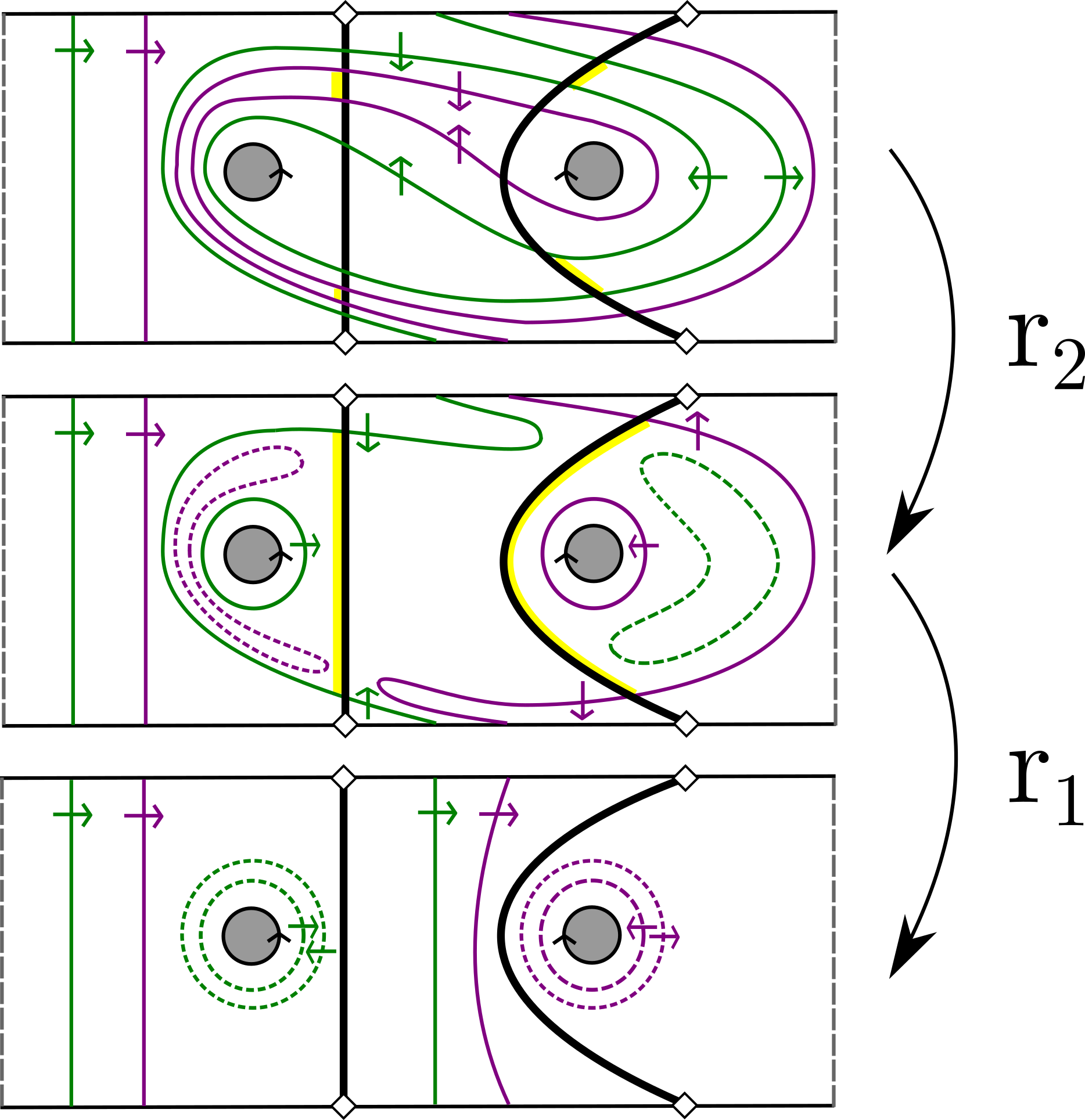
We still need to explain why $r_{n}\left(\left[h\right]\right)\in{\cal P}_{n-1}$. We do this through the following series of claims:

Claim 3.22.

$\kappa_{x}\left(h^{\prime\prime}\right)=1$ for all $x\in B$ .

?proofname?.

It is clear that step $\left(i\right)$ of Definition 3.21 does not alter $\kappa_{x}$, so $\kappa_{x}\left(h^{\prime}\right)=1$. It remains to show that for every $x\in B$ and $j\in\left[1\right]$, some $\left(x,j\right)$-arc/curve survives step $\left(ii\right)$. We remark that this is clear if there is some $\left(x,j\right)$-arc in $h$, because $r_{n}$ does not modify $h$ near $\partial\Sigma$. It is less clear, however, when there are only $\left(x,j\right)$-curves.

Let $\beta$ be some $\left(x,j\right)$-arc or $\left(x,j\right)$-curve of $h$, and consider $O_{1}$, the $o$-zone of $h$ touching $\beta$. All depth-$n$ leaves of $h$ are contained inside $o$-zones (recall our ongoing assumption in the proofs that $n$ is even), and the leaves inside $O_{1}$ cut it in step $\left(i\right)$ to smaller $o$-zones of $h^{\prime}$, separated by “$z$-tunnels” along the leaves of depth n. Let ${\cal O}_{\left(x,j\right)}$ denote the collection of $o$-zones of $h^{\prime}$ which are contained in $O_{1}$ and which are removed in step $\left(ii\right)$ because they contain no marked points and have only $\left(x,j\right)$-arcs/curves along their boundary. If ${\cal O}_{\left(x,j\right)}$ is empty, we are done, as the $\left(x,j\right)$-arcs/curves which are the traces of $\beta$ survive in $h^{\prime\prime}$. So assume ${\cal O}_{\left(x,j\right)}$ is non-empty. It cannot include all the $o$-zones of $h^{\prime}$ contained in $O_{1}$, because this would mean that $O_{1}$ itself is redundant. Thus, there must be some $o$-zone $O_{2}\in{\cal O}_{\left(x,j\right)}$ which borders, through a depth-$n$ leaf, some $o$-zone $O_{3}\notin{\cal O}_{\left(x,j\right)}$ of $h^{\prime}$ which is contained in $O_{1}$. Since the leaf separating $O_{2}$ and $O_{3}$ has $\left(x,j\right)$-arcs/curves on both sides (in $h^{\prime}$), $O_{3}$ has some bounding $\left(x,j\right)$-arc/curve, which survives step $\left(ii\right)$. ∎

We have not shown yet that $r_{n}\left(\left[h\right]\right)\in{\cal L}$: it remains to prove that $h^{\prime\prime}$ is loose, but the following claim is the analog of saying that $\left[h\right]\preceq_{{\cal L}}\left[h^{\prime\prime}\right]$:

Claim 3.23.

There is a transverse map $g$ for $\left(\Sigma,f\right)$ with $\kappa_{x}=3$ for all $x$, so that forgetting $\left(x,0\right)$ and $\left(x,3\right)$ for all $x$ yields a map in $\left[h\right]$ and forgetting $\left(x,1\right)$ and $\left(x,2\right)$ for all $x$ yields a map in $\left[h^{\prime\prime}\right]$.

?proofname?.

First, construct a transverse map $g$ with $\kappa_{x}=3$ by duplicating the arcs and curves of $h$, so that the $\left(x,0\right)$-arcs/curves are isotopic to the $\left(x,1\right)$-arcs/curves, and likewise with $\left(x,2\right)$ isotopic to $\left(x,3\right)$. Since the $H$-moves in step $\left(i\right)$ of Definition 3.21 are performed in $o$-zones (recall our assumption that $n$ is even), we can perform them for $g$, in which they involve only arcs/curves with color from $\bigcup_{x}\left\{\left(x,0\right),\left(x,3\right)\right\}$ and occur inside $o$-zones. The resulting map, call it $g^{\prime}$, shows the analog of $h\preceq_{{\cal L}}h^{\prime}$. Finally, the $o$-zones of $g^{\prime}$ are identical (up to homotopy) to those of $h^{\prime}$, so step $\left(ii\right)$ can be performed in $g^{\prime}$ by removing all redundant $o$-zones of $g^{\prime}$. The resulting map, $g^{\prime\prime}$, is still transverse with parameters $\kappa_{x}=3$ for all $x$ by Claim 3.22, and is the map we need to establish the claim. ∎

Lemma 3.24.

$r_{n}\left(\left[h\right]\right)\in{\cal L}$.

?proofname?.

We need to show that $h^{\prime\prime}$ is loose, namely that it abides to Restrictions 1 and 2. Neither step $\left(i\right)$ nor step $\left(ii\right)$ from Definition 3.21 change $h$ near $\partial\Sigma$, so $h^{\prime\prime}$ abides to Restriction 2 because so does $h$. It remains to show there are no “redundant” zones in $h^{\prime\prime}$, namely, no zones which violate Restriction 1. Note that the removal of redundant $o$-zones of $h^{\prime}$ in step $\left(ii\right)$ enlarges $z$-zones and possibly merges several $z$-zones into one, but it does not create new $o$-zones nor does it affect other existing $o$-zones. So the remaining $o$-zones are not redundant.

As for $z$-zones, we use the map $g^{\prime\prime}$ from Claim 3.23. We claim that $g^{\prime\prime}$ has no redundant $z$-zones. Clearly, $g^{\prime\prime}$ has no $\left(x,1\right)$-redundant zone, because these are exactly the $\left(x,0\right)$-zones of $h$, which abide to Restriction 1. Note that every $\left(x,0\right)$-arc/curve of $g^{\prime\prime}$ is parallel, at least in some segments, to $\left(x,1\right)$-arcs/curves (by the nature of $H$-moves). Hence, every $\left(x,0\right)$-zone of $g^{\prime\prime}$ must have some bounding $\left(x,1\right)$-arc/curve. Therefore, a redundant $\left(x,0\right)$-zone in $g^{\prime\prime}$ has only $\left(x,1\right)$-arcs/curves at its boundary, and is thus a redundant $o$-zone of $h$, a contradiction. That there are no redundant $\left(x,2\right)$-zones in $g^{\prime\prime}$ is analogous to the $\left(x,0\right)$ case.

Now, let $Z$ be an arbitrary $z$-zone of $h^{\prime\prime}$. Without loss of generality, there is some $\left(x,0\right)$-arc/curve of $h^{\prime\prime}$ at $\partial Z$. This $\left(x,0\right)$-arc/curve is at $\partial Z_{0}$ for some $\left(x,0\right)$-zone $Z_{0}$ of $g$ contained in $Z$. By the claim on $g$, this $Z_{0}$ borders some $\left(x,1\right)$-zone $Z_{1}\subset Z$ of $g$, which borders some $\left(x,2\right)$-zone $Z_{2}\subset Z$ of $g$. But $Z_{2}$ has some $\left(x,3\right)$-arc/curve of $g$ at its boundary, which is necessarily a $\left(x,1\right)$-arc/curve of $h^{\prime\prime}$ at the boundary of $Z$. Hence $Z$ does not violate Restriction 1. ∎

Corollary 3.25.

$r_{n}\left(\left[h\right]\right)\in{\cal P}_{n-1}$ and $\left[h\right]\preceq_{{\cal L}}r_{n}\left(\left[h\right]\right)$.

?proofname?.

It remains to show that $\mathrm{depth}\left(u_{\omega}\left(h^{\prime\prime}\right)\right)\leq n-1$ for all $\omega\in\Omega$. The $H$-moves of step $\left(i\right)$ in the definition of $r_{n}$ remove all the crossings between $\omega$ and arcs/curves of $h$ which cut out depth-$n$ leaves. It is thus clear that $\mathrm{depth}\left(u_{\omega}\left(h^{\prime}\right)\right)\leq n-1$. But whenever $\omega$ enters a redundant zone of $h^{\prime}$, it has to leave it through an arc/curve of the same color. So the effect of removing a redundant zone on the words $u_{w}\left(h^{\prime}\right)$ is performing reduction steps (omitting consecutive pairs of the type $P_{x}P_{x}$ or $Q_{x}Q_{x}$). Reduction moves cannot increase the depth of the word. ∎

After establishing that $r_{n}\colon{\cal P}_{n}\to{\cal P}_{n-1}$, our next goal is to use $r_{n}$ to obtain the sought-after deformation retract. We do this using the following general technique concerning posets:

A map $\varphi\colon P\to Q$ between posets which is order-preserving, in the sense that $p_{1}\leq_{P}p_{2}\Longrightarrow\varphi\left(p_{1}\right)\leq_{Q}\varphi\left(p_{2}\right)$, maps a chain $p_{0}<_{P}\ldots<_{P}p_{m}$ in $P$ to a, possibly “stuttering”, chain $\varphi\left(p_{0}\right)\leq_{Q}\ldots\leq_{Q}\varphi\left(p_{m}\right)$ in $Q$, so the set $\left\{\varphi\left(p_{0}\right),\ldots,\varphi\left(p_{m}\right)\right\}$ defines a simplex in the order complex $\left|Q\right|$. This allows the following natural induced map $\left|\varphi\right|\colon\left|P\right|\to\left|Q\right|$ between the order complexes:

$$\left|\varphi\right|\left(\sum\lambda_{i}p_{i}\right)=\sum\lambda_{i}\varphi\left(p_{i}\right).$$ (3.2)

Lemma 3.26.

Let $P$ be a subposet of the poset $Q$. Assume that $\varphi\colon Q\to P$ satisfies the following three conditions:

• $\varphi$ is order-preserving

• $\varphi$ is a retract, i.e. $f\Big{|}_{P}\equiv\mathrm{id}$

• $\varphi\left(q\right)\leq q$ for all $q\in Q$, or $\varphi\left(q\right)\geq q$ for all $q\in Q$

Then $\left|\varphi\right|\colon\left|Q\right|\to\left|P\right|$ is a strong deformation retract.

By a strong deformation retract we mean that there is a homotopy of $\left|\varphi\right|$ with the identity on $\left|Q\right|$ which fixes $\left|P\right|$ pointwise throughout the homotopy.

?proofname?.

Recall that a map $\psi$ between posets is called a poset-morphism if it is order preserving. If $\psi\colon P\to Q$ is a poset morphism, we let $\left|\psi\right|$ denote the induced map $\left|\psi\right|\colon\left|P\right|\to\left|Q\right|$ defined as in (3.2). If $P$ and $Q$ are posets, $\psi_{0},\psi_{1}\colon P\to Q$ are poset morphisms, and $\psi_{0}\left(p\right)\leq\psi_{1}\left(p\right)$ for every $p\in P$, then $\left|\psi_{0}\right|$ and $\left|\psi_{1}\right|$ are homotopic. Indeed, let $\left\{0\leq 1\right\}$ denote the poset with two comparable elements $0$ and 1. Define a map $\left(\psi_{0},\psi_{1}\right)\colon P\times\left\{0\leq 1\right\}\to Q$ by $\left(p,0\right)\mapsto\psi_{0}\left(p\right)$ and $\left(p,1\right)\mapsto\psi_{1}\left(p\right)$. This is clearly a poset-morphism by the assumptions, so it induces a continuous map

$$\left|\left(\psi_{0},\psi_{1}\right)\right|\colon\left|P\times\left\{0\leq 1\right\}\right|\to\left|Q\right|.$$

By Fact 3.11, there is an homeomorphism

$$\left|P\times\left\{0\leq 1\right\}\right|\overset{\cong}{\to}\left|P\right|\times\left|\left\{0\leq 1\right\}\right|=\left|P\right|\times\left[0,1\right],$$

so we get that $\left|\left(\psi_{0},\psi_{1}\right)\right|$ is a continuous map $\left|P\right|\times\left[0,1\right]\to\left|Q\right|$. Because $\left|\left(\psi_{0},\psi_{1}\right)\right|\Big{|}_{\left|P\times\left\{0\right\}\right|}\equiv\left|\psi_{0}\right|$ and $\left|\left(\psi_{0},\psi_{1}\right)\right|\Big{|}_{\left|P\times\left\{1\right\}\right|}\equiv\left|\psi_{1}\right|$, the map $\left|\left(\psi_{0},\psi_{1}\right)\right|$ is the sought-after homotopy. (This result appears in [Qui73, Section 1.3].)

Note that the map $\varphi\colon Q\to Q$ in the statement of the lemma and the identity $\mathrm{id}\colon Q\to Q$ satisfy the conditions regarding $\psi_{0}$ and $\psi_{1}$ above. Hence $\left|\varphi\right|$ is homotopic to the identity. The fact that the homotopy fixes $\left|P\right|$ pointwise follows from the fact that the homotopy above does not move the points where $\psi_{0}$ and $\psi_{1}$ agree. Namely, if $P_{0}\subseteq P$ is the subposet where $\psi_{0}\left(p\right)=\psi_{1}\left(p\right)$, then $\left|\left(\psi_{0},\psi_{1}\right)\right|\left(x,t\right)=\psi_{0}\left(x\right)=\psi_{1}\left(x\right)$ for every $x\in\left|P_{0}\right|$ and $t\in\left[0,1\right]$. ∎

Proposition 3.27.

The map $r_{n}\colon{\cal P}_{n}\to{\cal P}_{n-1}$ satisfies the conditions of Lemma 3.26 and so defines a strong deformation retract

$$\left|r_{n}\right|\colon\left|{\cal P}_{n}\right|\to\left|{\cal P}_{n-1}\right|.$$

?proofname?.

We already proved above that for $n$ even, $\left[h\right]\preceq_{{\cal L}}r_{n}\left(\left[h\right]\right)$ which is the third assumption of Lemma 3.26. The second assumption is also clear: if $\left[h\right]\in{\cal P}_{n-1}$, then $h$ admits no depth-$n$ leaves in $\Omega$, and therefore in Definition 3.21, $h=h^{\prime}=h^{\prime\prime}$. It remains to show that $r_{n}$ is order-preserving.

Let $h_{1}$ and $h_{2}$ be transverse maps so that $\left[h_{1}\right],\left[h_{2}\right]\in{\cal P}_{n}$, with $\left[h_{1}\right]\preceq_{{\cal L}}\left[h_{2}\right]$, and assume that $g$ is a transverse map $g$ with $\kappa_{x}=3$ for all $x$, so that $h_{1}$ and $h_{2}$ are obtained by forgetting the exterior and interior, respectively, two transversion points for every letter $x$. We also assume $g$ is in minimal position with respect to $\Omega$. For $\omega\in\Omega$, the words $u_{\omega}\left(h_{1}\right)$ and $u_{\omega}\left(h_{2}\right)$ are very much dependent: they can be constructed simultaneously by following the path $g\left(\omega\right)$ in ${\textstyle\bigvee^{r}S^{1}}$, and adding a letter to $u_{\omega}\left(h_{1}\right)$ whenever $g\left(\omega\right)$ crosses some $\left(x,1\right)$ or $\left(x,2\right)$ point, and a letter to $u_{\omega}\left(h_{2}\right)$ whenever $g\left(\omega\right)$ crosses some $\left(x,0\right)$ or $\left(x,3\right)$ point. This description shows that whenever $\omega$ visits an $o$-zone or an $\left(x,1\right)$-zone of $g$, the prefix of the two words until that point has the same reduced form and, in particular, the same length.

Consider a depth-$n$ leaf $\gamma$ of $h_{1}$ in $\omega$. The beginning of $\gamma$ is at a crossing point of $\omega$ with some $\left(x,j\right)$-arc/curve of $g$ with $x\in B$ and $j\in\left\{1,2\right\}$, in which $\omega$ leaves an $\left(x,1\right)$-zone of $g$ and enters some $\left(x,0\right)$- or $\left(x,2\right)$-zone. Without loss of generality, assume that $\omega$ crosses some $\left(y,1\right)$-arc/curve with $y\in B$. The image $g\left(\gamma\right)$ is a closed path in ${\textstyle\bigvee^{r}S^{1}}$, based at $\left(y,1\right)$, which avoids the segments $\left[\left(x,1\right),\left(x,2\right)\right]$ for every $x\in B$ – see Figure 3.6.

?figurename? 3.6: The wedge ${\textstyle\bigvee^{r}S^{1}}$ when $r=2$, $B=\left\{x,y\right\}$. The marked points are the transversion points of a map $g$, with $\kappa_{x}\left(g\right)=\kappa_{y}\left(g\right)=3$. If $h_{1}$ is the transverse map obtained from $g$ by forgetting $\left(x,0\right),\left(x,3\right),\left(y,0\right),\left(y,3\right)$ and if $n$ is even, then a depth-$n$ leaf $\gamma$ of $h_{1}$ at some null-arc $\omega$ is contained in some $o$-zone of $h_{1}$, meaning that $g\left(\gamma\right)$ lives outside the broken segments in the figure.

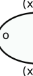
When one follows the prefix of the word $u_{\omega}\left(h_{2}\right)$ along $\gamma$, it is clear, therefore, that at the beginning of $\gamma$ it has length $n-1$. If it then crosses $\left(y,0\right)$, it has the same length as the prefix of $u_{\omega}\left(h_{1}\right)$ which is $n$. Then, it could seemingly cross, e.g., $\left(x,3\right)$ for some $x\in B$, but this would increase the length of the prefix of $u_{\omega}\left(h_{2}\right)$ to $n+1$, which is impossible as $\left[h_{2}\right]\in{\cal P}_{n}$. Hence $g\left(\gamma\right)$ can only cross the point $\left(y,0\right)$ back and forth. Every two consecutive such crossings define a depth-$n$ leaf of $h_{2}$ at $\omega$.

Therefore, in the notation of Definition 3.21, step $\left(i\right)$ can be performed in two phases: first, perform step $\left(i\right)$ for $h_{2}$, where the depth-$n$ leaves never cross any arcs/curves of $h_{1}$. Second, perform step $\left(i\right)$ for $h_{1}$: although a depth-$n$ leaf of $h_{1}$ may cross arcs/curves of $h_{2}$, the previous paragraph explains why it never crosses arcs/curves of $h_{2}^{\prime}$. The resulting $h_{1}^{\prime}$ and $h_{2}^{\prime}$ are compatible together in the sense there is $g^{\prime}$ with $\kappa_{x}=3$ as in the definition of the order on ${\cal L}$ (although, of course, $h_{1}^{\prime}$ and $h_{2}^{\prime}$ may not be in ${\cal L}$). See Figure 3.7.

?figurename? 3.7: On the left, a piece of a null-arc $\omega$ crosses some arcs/curves of $g$, the transverse map with $\kappa_{x}=3$ for all $x$ showing that $h_{1}\preceq_{{\cal L}}h_{2}$, both inside ${\cal P}_{n}$. The thick red part of $\omega$ is a depth-$n$ leaf $\gamma$ of $h_{1}$, which in $g$ is a segment of $\omega$ between two crossing-points with $\left(y,1\right)$-arcs/curves. Inside $\gamma$ there are two depth-$n$ leaves of $h_{2}$, which, in $g$, are two segments cut out by $\left(y,0\right)$-arcs/curves. The right hand side shows the result of step $\left(i\right)$ of Definition 3.21 on this local picture, where performing the single $H$-move for $h_{1}$ after the two $H$-moves of $h_{2}$ causes no collisions.

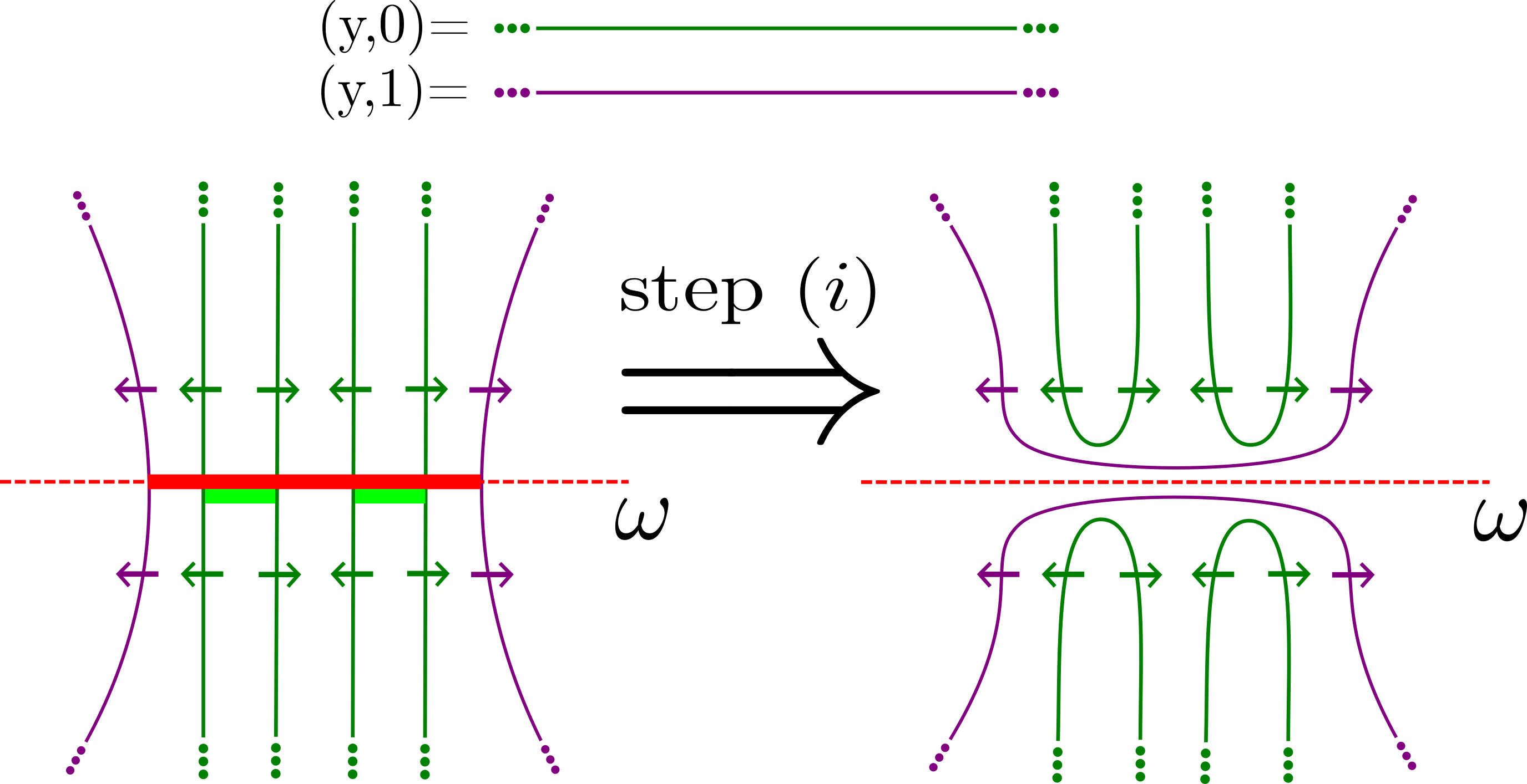
In step $\left(ii\right)$ of Definition 3.21 we now remove redundant $o$-zones of $h_{1}^{\prime}$ and of $h_{2}^{\prime}$. Since the $o$-zones of $h_{2}^{\prime}$ and those of $g^{\prime}$ coincide, removing redundant $o$-zones of $h_{2}^{\prime}$ is equivalent to removing redundant $o$-zones of $g^{\prime}$ and keeps the structure of $g^{\prime}$ as a legal transverse map with $\kappa_{x}=3$ for all $x$. Denote the resulting map by $\overline{g^{\prime}}$. However, we still need to show that removing redundant $o$-zones of $h_{1}^{\prime}$ does not cause a problem, namely, that any redundant $o$-zone of $h_{1}^{\prime}$ does not contain any curves of $h_{2}^{\prime\prime}$, which are the same as $\left(x,0\right)$- or $\left(x,3\right)$-curves of $\overline{g^{\prime}}$ for any $x\in B$.

Indeed, let $O$ be a redundant $o$-zone of $h_{1}^{\prime}$. Without loss of generality it is bounded by outgoing $\left(y,1\right)$-curves of $\overline{g^{\prime}}$. Assume there is some curve of $h_{2}^{\prime\prime}$ inside $O$ which is not a $\left(y,0\right)$-curve of $\overline{g^{\prime}}$, say, an $\left(x,3\right)$-curve of $\overline{g^{\prime}}$. The negative side of this $\left(x,3\right)$-curve cannot be a redundant $\left(x,2\right)$-zone of $\overline{g^{\prime}}$, because then it would be a redundant $z$-zone of $h_{2}^{\prime\prime}$ which is impossible by Lemma 3.24. Thus, this $\left(x,2\right)$-zone of $\overline{g^{\prime}}$ must have some $\left(x,2\right)$-arc/curve at its boundary, a contradiction to the assumption that $O$ is redundant. We conclude that $O$ may only contain $\left(y,0\right)$-curves of $\overline{g^{\prime}}$. But then, on their negative side, these curves must bound a redundant zone (there cannot be marked points from $V_{o}$ inside as $O$ is redundant), and thus should have been removed in step $\left(ii\right)$ for $h_{2}$. Therefore, step $\left(ii\right)$ for $h_{1}^{\prime}$ can be performed on $\overline{g^{\prime}}$ without violating any rule, and the resulting map, $g^{\prime\prime}$, shows that $r_{n}\left(h_{1}\right)=\left[h_{1}^{\prime\prime}\right]\preceq_{{\cal L}}\left[h_{2}^{\prime\prime}\right]=r_{n}\left(\left[h_{2}\right]\right)$. ∎

Proof of Proposition 3.20.

To get a deformation retract of $\left|{\cal L}\right|$ to $\left|{\cal L}_{\Omega}\right|$ we perform $\left|r_{n}\right|$ at time $\left[\frac{1}{2^{n}},\frac{1}{2^{n-1}}\right]$. We remark that the fact that $\left|r_{n}\right|$ is a strong deformation retract, namely, keeps $\left|{\cal P}_{n-1}\right|$ fixed pointwise, guarantees that the total deformation retract on $\left|{\cal L}\right|$ is well defined. ∎

4 The action of $\mathrm{MCG}(f)$ on the complex of transverse maps

In this section we prove our main results: Theorems 1.4, 1.6 and 1.7. We begin with some background on $L^{2}$-Euler characteristics.

4.1 $L^{2}$-Betti numbers and $L^{2}$-Euler characteristics

We now define the $L^{2}$-invariants of groups that appear in our main theorem, although, for the sake of the proofs, one can use Theorem 4.2, Lemma 4.3 and Theorem 4.4 as black boxes.

The following definitions and properties are all found in the book of Lück [Lüc02]; many of the ideas we discuss originate from the paper of Cheeger and Gromov [CG86]. Throughout this subsection, $G$ is a discrete group.

Definition 4.1 ([Lüc02, Def. 1.25]).

A $G$-CW-complex is a CW-complex with a cellular action of $G$ such that if an element of $G$ fixes an open cell, it acts as the identity on that open cell.

Following [Lüc02, Def. 1.1], the group von Neumann algebra $\mathcal{N}(G)$ is defined to be the space of $G$-equivariant bounded operators from $\ell^{2}(G)$ to itself. Here $\ell^{2}(G)$ is given the standard Hermitian inner product making it a Hilbert space. Now suppose $X$ is a $G$-CW-complex. Denote by $C_{*}^{\mathrm{sing}}\left(X\right)$ the singular chain complex of $X$. This is a complex of left $\mathbb{Z}G$-modules. Giving $\mathcal{N}(G)$ the structure of an $\left(\mathcal{N}(G),\mathbb{Z}G\right)$-bimodule, we can form a chain complex

$$\ldots\xrightarrow{d_{p+1}}\mathcal{N}(G)\otimes_{\mathbb{Z}G}C_{p}^{\mathrm{sing}}(X)\xrightarrow{d_{p}}\mathcal{N}(G)\otimes_{\mathbb{\mathbb{Z}}G}C_{p-1}^{\mathrm{sing}}(X)\xrightarrow{d_{p-1}}\ldots$$

of $\mathcal{N}(G)$-modules. This is a Hilbert chain complex in the terminology of [Lüc02, Def. 1.15]. In particular, each piece $\mathcal{N}(G)\otimes_{\mathbb{Z}G}C_{p}^{\mathrm{sing}}(X)$ is a Hilbert module for $\mathcal{N}(G)$ as defined in [Lüc02, Def. 1.5], $\mathcal{N}(G)\otimes_{\mathbb{Z}G}C_{p}^{\mathrm{sing}}(X)$ is a Hilbert space, and the boundary maps are bounded $G$-equivariant operators. The $L^{2}$-homology of the pair $\left(X,G\right)$ we denote by $H_{*}^{(2)}\left(X;G\right)$ and define by

$$H_{p}^{(2)}\left(X;G\right)\overset{\mathrm{def}}{=}\frac{\ker(d_{p})}{\mathrm{closure}(\mathrm{image}(d_{p+1}))},$$

cf. [Lüc02, Def. 6.50, Def. 1.16]. Each of these homology groups are themselves Hilbert $\mathcal{N}(G)$-modules. Any $\mathcal{N}(G)$-module $M$ has an associated dimension in $[0,\infty]$ called the von Neumann dimension and denoted by $\dim_{\mathcal{N}(G)}(M)$ [Lüc02, Def 6.20]. The $L^{2}$-Betti numbers of the pair $\left(X,G\right)$ are defined by

$$b_{p}^{(2)}\left(X,G\right)\overset{\mathrm{def}}{=}\dim_{\mathcal{N}(G)}H_{p}^{(2)}\left(X;G\right)\in[0,\infty].$$

If

$$\sum_{p\in\mathbb{Z}_{\geq 0}}b_{p}^{(2)}\left(X,G\right)<\infty$$ (4.1)

then we can also define the $L^{2}$-Euler characteristic of the pair $\left(X,G\right)$ to be

$$\chi^{(2)}\left(X,G\right)=\sum_{p\in\mathbb{Z}_{\geq 0}}(-1)^{p}\cdot b_{p}^{(2)}\left(X,G\right)\in\mathbb{R}.$$

If $EG$ is a contractible $G$-CW-complex with a free action of $G$ then we define

$$b_{p}^{(2)}\left(G\right)\overset{\mathrm{def}}{=}b_{p}^{(2)}\left(EG,G\right)$$

and if moreover (4.1) holds for $X=EG$, then we also define as in [Lüc02, Def. 6.79] the $L^{2}$-Euler characteristic of $G$ to be

$$\chi^{(2)}\left(G\right)\overset{\mathrm{def}}{=}\chi^{(2)}\left(EG,G\right).$$

Since $EG$ is unique up to $G$-equivariant homotopy equivalence, it follows for example from [Lüc02, Theorem 6.54] that the quantities $b_{p}^{(2)}\left(G\right),\chi^{(2)}\left(G\right)$ only depend on $G$. The existence and $G$-homotopy uniqueness of $EG$ is discussed in [Lüc02, pg. 33] with references therein to [tD72, tD87].

Assume $X$ is an arbitrary $G$-CW-complex. If $c$ is a cell of $X$ write $G_{c}$ for the isotropy group (stabilizer) of $c$ in $G$. As in [Lüc02, §6.6.1], we consider the quantities

$$\left|G_{c}\right|^{-1}$$

where we set $\left|G_{c}\right|^{-1}=0$ if $G_{c}$ is infinite. We define following [Lüc02, Def 6.79]

$$m\left(X,G\right):=\sum_{[c]\in G\backslash X}\left|G_{c}\right|^{-1}\in[0,\infty].$$

Theorem 4.2 ([Lüc02, Thm. 6.80(1)]).

If $m\left(X,G\right)$ is finite then the sum of $b_{p}^{(2)}\left(X,G\right)$ is finite and, moreover,

$$\chi^{(2)}\left(X,G\right)=\sum_{[c]\in G\backslash X}\left(-1\right)^{\dim c}\left|G_{c}\right|^{-1}.$$ (4.2)

Following [Lüc02, Def. 7.1] let $\mathcal{B}_{\infty}$ denote the class of groups $G$ for which $b_{p}\left(G\right)=0$ for all $p\in\mathbb{Z}_{\geq 0}$.

Lemma 4.3.

If $X$ is a contractible $G$-CW-complex, and for all cells $c$ of $X$ the isotropy group $G_{c}$ is either finite or in $\mathcal{B}_{\infty}$, then

$$b_{p}^{(2)}\left(X,G\right)=b_{p}^{(2)}\left(G\right),\quad p\in\mathbb{Z}_{\geq 0}.$$

Hence if also $m\left(X,G\right)$ is finite then $\chi^{(2)}\left(X,G\right)=\chi^{(2)}\left(G\right)$.

?proofname?.

This is [Lüc02, Exercise 6.20]. It can be proved by combining [Lüc02, Thm 6.54 (2) and (3)], and referring to Theorem 4.2 for the statement about Euler characteristics. ∎

To use Lemma 4.3 we need to have a source of groups lying in $\mathcal{B}_{\infty}$. The following theorem is essentially due to Cheeger and Gromov (cf. [CG86, Corollary 0.6]). The precise statement we need can be deduced from [Lüc02, Theorem 7.2, items (1) and (2)]. Recall that a discrete group is called amenable if it has a finitely additive left invariant probability measure.

Theorem 4.4 (Cheeger-Gromov).

If $G$ is a discrete group containing a normal infinite amenable subgroup then $G\in\mathcal{B}_{\infty}$.

4.2 The complex of transverse maps as a $\mathrm{MCG}\left(f\right)$-CW-complex

The stabilizer $\mathrm{MCG}\left(f\right)$ of $f$ in $\mathrm{MCG}\left(\Sigma\right)$ acts on the poset ${\cal T}={\cal T}\left(\Sigma,f\right)$ by precomposition: if $\left[\rho\right]\in\mathrm{MCG}\left(f\right)$ and $\left[g\right]\in{\cal T}$ with parameters $\kappa$, then $\left[\rho\right].\left[g\right]=\left[g\circ\rho^{-1}\right]$ is an element of ${\cal T}$ with the same $\kappa$: indeed, $g\circ\rho^{-1}$ is a transverse map realizing $f$ with the exact same transversion points as $g$. This action is obviously an order preserving action: if $\left[g_{1}\right]\preceq\left[g_{2}\right]$ then $\left[\rho\right].\left[g_{1}\right]\preceq\left[\rho\right].\left[g_{2}\right]$.

We now show that this action on ${\cal T}$ turns its geometric realization into a $\mathrm{MCG}\left(f\right)$-$CW$-complex, as in Definition 4.1. The properties mentioned above of the action of $\mathrm{MCG}\left(f\right)$ on the poset ${\cal T}$ guarantee that this is the case for $\left|{\cal T}\right|$, the order complex of ${\cal T}$ (see Page 3.9 for the definition of $\left|{\cal T}\right|$). We claim this is also the case for the polysimplicial complex $\left|{\cal T}\right|_{\mathrm{poly}}$:

Lemma 4.5.

Let $[(\Sigma,f)]\in\mathsf{Surfaces}(w_{1},\ldots,w_{\ell})$. Let $\Gamma=\mathrm{MCG}(f)$. The action of $\Gamma$ on ${\cal T}={\cal T}(\Sigma,f)$ makes $\left|{\cal T}\right|_{\mathrm{poly}}$ into a $\Gamma$-CW-complex.

?proofname?.

If $\left[\rho\right]\in\Gamma$ fixes $[g]\in{\cal T}$ we need to show $\left[\rho\right]$ cannot permute the faces of $\mathrm{polysim\left(\left[g\right]\right)}$. But $\left[g\circ\rho^{-1}\right]=\left[g\right]$ means there is an isotopy of transverse maps between $g$ and $g\circ\rho^{-1}$. In such an isotopy, the $\sum_{x\in B}\left(\kappa_{x}\left(g\right)+1\right)$ points of transversion in ${\textstyle\bigvee^{r}S^{1}}$ may move around, but away from the wedge point $o$, and without collisions. This means that their order on each circle of ${\textstyle\bigvee^{r}S^{1}}$ is preserved. In particular, for every $x\in B$ and $j\in\left[\kappa_{x}\left(g\right)\right]$, the isotopy takes the $\left(x,j\right)$ point of $g$ to the $\left(x,j\right)$ point of $g\circ\rho^{-1}$, and the collection of $\left(x,j\right)$-arcs/curves of $g$ to the collection of $\left(x,j\right)$-arcs/curves of $g\circ\rho^{-1}$. Thus, $\left[\rho\right]$ necessarily preserves every face of $\mathrm{polysim}\left(\left[g\right]\right)$. ∎

Definition 4.6.

We define ${\cal T}_{\infty}={\cal T}_{\infty}(\Sigma,f)$ to be the subposet of ${\cal T}={\cal T}\left(\Sigma,f\right)$ consisting of classes of transverse maps $\left[g\right]$ in ${\cal T}$ that do not fill $\Sigma$.

Recall that $\left[g\right]$ fills $\Sigma$ if its $o$-zones and $z$-zones are all topological discs. This means, in particular, that the preimage of every transversion point contains only arcs (and no curves).

Our notation ${\cal T}_{\infty}$ is in analogy to Harer’s use of $A_{\infty}$ in [Har86, Har85] for the subcomplex of the arc complex consisting of arc systems that do not cut the surface into discs; Harer used this complex in [Har86] to construct a Borel-Serre type bordification of Teichmüller space. This had previously been done by Harvey [Har81] using the complex of curves. These bordifications are closely related to the Deligne-Mumford compactification [DM69] of the moduli space of curves (see [Mon08, Remark 2.5]).

We define $\left|{\cal T}_{\infty}\right|_{\mathrm{poly}}$ to be the polysimplicial subcomplex of $\left|{\cal T}\right|_{\mathrm{poly}}$ consisting of polysimplices in ${\cal T}_{\infty}$. It is clear that $\left|{\cal T}_{\infty}\right|_{\mathrm{poly}}$ is indeed a subcomplex of $\left|{\cal T}\right|_{\mathrm{poly}}$ since if the arcs of $\left[g\right]$ do not cut $\Sigma$ into discs then neither do the arcs of $\left[g^{\prime}\right]$ obtained from $g$ by forgetting points of transversion.

Lemma 4.7.

$\mathrm{MCG}(f)$ acts freely on ${\cal T}\setminus{\cal T}_{\infty}$.

?proofname?.

If $\left[\rho\right]$ in $\mathrm{MCG}(f)$ fixes an isotopy class $\left[g\right]$ of filling transverse maps then we can assume $\rho$ fixes all the arcs of $g$, so restricts to mapping classes on each of the zones of $g$, which are all discs. The Alexander Lemma [FM12, Lemma 2.1] implies these mapping classes must be trivial, so $\rho$ is homotopic to the identity on each zone of $g$, hence overall. ∎

So the isotropy groups $\mathrm{MCG}\left(f\right)_{\left[g\right]}$ are trivial for $\left[g\right]\in{\cal T}\setminus{\cal T}_{\infty}$. The following lemma shows that for any other element of ${\cal T}$, the isotropy groups are not only infinite, but also have vanishing $L^{2}$-Betti numbers:

Lemma 4.8.

Let $\Gamma=\mathrm{MCG}(f)$. If $\left[g\right]\in{\cal T}_{\infty}$ then the isotropy group $\Gamma_{\left[g\right]}$ of $\left[g\right]$ are in $\mathcal{B}_{\infty}$.

?proofname?.

Fix a representative transverse map $g$ for $\left[g\right]$. Let $\mathcal{C}$ denote a set of disjoint simple closed curves, where for every zone of $g$ we add a simple closed curve parallel to every boundary component of that zone to $\mathcal{C}$, and we think of the curves as drawn inside the zones of $g$ they come from. If $g$ contains curves in the preimages of points of transversion, then this process can add to $\mathcal{C}$ multiple copies of isotopy classes of simple closed curves, but this does not matter.

Because $\mathcal{C}$ is drawn in the zones of $g$, then a Dehn twist in any element of $\mathcal{C}$ belongs to $\Gamma$. Let $N$ be the subgroup of $\Gamma$ generated by Dehn twists in elements of $\mathcal{C}$. This group is isomorphic to $\mathbf{\mathbf{Z}}^{r}$ for some $r\geq 0$ because the curves in ${\cal C}$ are disjoint. In fact, $r\geq 1$ since by assumption, some zone of $g$ is not a topological disc, and hence has a boundary component which does not bound a disc, so gives rise to a non-trivial Dehn twist. To see that $N$ is normal in $\Gamma_{\left[g\right]}$, note that any mapping class in $\Gamma_{\left[g\right]}$ can be taken to permute the zones of $g$. Hence $\Gamma_{\left[g\right]}$ permutes the isotopy classes of curves in $\mathcal{C}$. Therefore the conjugation by $\left[\rho\right]\in\Gamma_{\left[g\right]}$ of any Dehn twist in an element of $\mathcal{C}$ is another Dehn twist in an element of $\mathcal{C}$.

It was proved by von Neumann [von29] that $\mathbb{Z}^{r}$ is amenable, hence $\Gamma_{\left[g\right]}$ contains a normal infinite amenable subgroup. The statement of the lemma now follows from Theorem 4.4. ∎

4.3 Proof of Theorem 2.16

Fix $[(\Sigma,f)]\in\mathsf{Surfaces}(w_{1},\ldots,w_{\ell})$ and let $\Gamma=\mathrm{MCG}\left(f\right)$. Recall that Theorem 2.16 states that $\chi^{\left(2\right)}\left(\Gamma\right)$ is well-defined and is given by a finite alternating sum over the set $\mathrm{\overline{MATCH}}^{*}\left(w_{1},\ldots,w_{\ell};\Sigma,f\right)$ of matchings of the letters of $w_{1},\ldots,w_{\ell}$. There is a natural map from elements of ${\cal T}\setminus{\cal T}_{\infty}$ to $\mathrm{\overline{MATCH}}^{*}\left(w_{1},\ldots,w_{\ell};\Sigma,f\right)$:

Definition 4.9.

Define a map

$$\widetilde{\mathbf{match}}\colon{\cal T}\setminus{\cal T}_{\infty}\to\mathrm{\overline{MATCH}}^{*}\left(w_{1},\ldots,w_{\ell}\right)$$

as follows. The $\left(x,j\right)$-arcs of $\left[g\right]\in{\cal T}\setminus{\cal T}_{\infty}$ define a matching $\sigma_{x,j}$ between the instances of $x^{+1}$ in $w_{1},\ldots,w_{\ell}$ and the instances of $x^{-1}$. Define $\widetilde{\mathbf{match}}\left(\left[g\right]\right)$ to be the element $\sigma\in\mathrm{\overline{MATCH}}^{\kappa\left(g\right)}\left(w_{1},\ldots,w_{\ell}\right)$ consisting of the matchings $\left\{\sigma_{x,j}\right\}_{x\in B,j\in\left[\kappa_{x}\right]}$.

We remark that if $\sigma=\widetilde{\mathbf{match}}\left(\left[g\right]\right)$ then indeed $\sigma_{x,j}\neq\sigma_{x,j+1}$ for $x\in B,j<\kappa_{x}$: this is guaranteed by Restriction 3 and the fact that the arcs of $g$ cut $\Sigma$ into discs.

Lemma 4.10.

The map $\widetilde{\mathbf{match}}$ descends to a bijection

$$\mathbf{match}\colon\leavevmode\nobreak\ \leavevmode\nobreak\ \mathrm{MCG}(f)\backslash\left({\cal T}\setminus{\cal T}_{\infty}\right)\stackrel{{\scriptstyle\cong}}{{\longrightarrow}}\mathrm{\overline{MATCH}}^{*}\left(w_{1},\ldots,w_{\ell};\Sigma,f\right).$$ (4.3)

?proofname?.

It is obvious that $\widetilde{\mathbf{match}}$ is invariant under the action of $\mathrm{MCG}\left(f\right)$, hence $\mathbf{match}$ is well defined. Since every element $\left[g\right]\in{\cal T}\setminus{\cal T}_{\infty}$ fills $\Sigma$ (its arcs cut $\Sigma$ into discs), it is clear that $\left(\Sigma,f\right)\sim\left(\Sigma_{\sigma},f_{\sigma}\right)$ where $\sigma=\widetilde{\mathbf{match}}\left(\left[g\right]\right)$, using a homeomorphism $\rho\colon\Sigma\to\Sigma_{\sigma}$ taking $g$ to the transverse map $f_{\sigma}$ (so $g\circ\rho^{-1}$ and $f_{\sigma}$ are isotopic as transverse maps - recall Definitions 2.7 and 2.11). This shows $\left(i\right)$ that $\widetilde{\mathbf{match}}\left(\left[g\right]\right)$ indeed belongs to $\mathrm{\overline{MATCH}}^{*}\left(w_{1},\ldots,w_{\ell};\Sigma,f\right)$ (and not only to $\mathrm{\overline{MATCH}}^{*}\left(w_{1},\ldots,w_{\ell}\right)$), and $\left(ii\right)$ that if $\widetilde{\mathbf{match}}\left(\left[g_{1}\right]\right)=\widetilde{\mathbf{match}}\left(\left[g_{2}\right]\right)$ then $\left[g_{1}\right]$ and $\left[g_{2}\right]$ are in the same $\mathrm{MCG}\left(f\right)$-orbit of ${\cal T}\setminus{\cal T}_{\infty}$, hence (4.3) is injective.

Finally, to see (4.3) is surjective, notice that for every $\sigma\in\mathrm{\overline{MATCH}}^{*}\left(w_{1},\ldots,w_{\ell};\Sigma,f\right)$, if $\rho$ is the homeomorphism showing the equivalence of $\left(\Sigma,f\right)\sim\left(\Sigma_{\sigma},f_{\sigma}\right)$ as above, then $\left[f_{\sigma}\circ\rho\right]\in{\cal T}\setminus{\cal T}_{\infty}$, and its image through $\widetilde{\mathbf{match}}$ is $\sigma$. ∎

It follows from Claim 2.10 that $\mathrm{\overline{MATCH}}^{*}\left(w_{1},\ldots,w_{\ell};\Sigma,f\right)$ is finite, hence:

Corollary 4.11.

There are finitely many $\mathrm{MCG}(f)$-orbits in ${\cal T}\setminus{\cal T}_{\infty}$.

We can now prove Theorem 2.16.

Proof of Theorem 2.16.

The polysimplicial complex $\left|{\cal T}\right|_{\mathrm{poly}}$ is a $\Gamma$-$CW$-complex for $\Gamma=\mathrm{MCG}\left(f\right)$ by Lemma 4.5. The isotropy groups of $\Gamma$ in its action on $\left|{\cal T}\right|_{\mathrm{poly}}$ are either trivial if $\left[g\right]\in{\cal T}\setminus{\cal T}_{\infty}$ (Lemma 4.7) or infinite if $\left[g\right]\in{\cal T}_{\infty}$ (Lemma 4.8). Since $\Gamma\backslash\left({\cal T}\setminus{\cal T}_{\infty}\right)$ is finite (Corollary 4.11), we have that

$$m\left(\left|{\cal T}\right|_{\mathrm{poly}},\Gamma\right)=\sum_{\left[g\right]\in\Gamma\backslash{\cal T}}\left|\Gamma_{[g]}\right|^{-1}=\sum_{\left[g\right]\in\Gamma\backslash\left({\cal T}\setminus{\cal T}_{\infty}\right)}\left|\Gamma_{[g]}\right|^{-1}$$

is finite. From Theorem 4.2 we deduce that $\chi^{\left(2\right)}\left(\left|{\cal T}\right|_{\mathrm{poly}},\Gamma\right)$ is well defined and given by

$$\chi^{\left(2\right)}\left(\left|{\cal T}\right|_{\mathrm{poly}},\Gamma\right) = \sum_{\left[g\right]\in\Gamma\backslash{\cal T}}\left(-1\right)^{\dim\left(\mathrm{polysim}\left[g\right]\right)}\left|\Gamma_{[g]}\right|^{-1}=\sum_{\left[g\right]\in\Gamma\backslash\left({\cal T}\setminus{\cal T}_{\infty}\right)}\left(-1\right)^{\left|\kappa\left(g\right)\right|}\left|\Gamma_{[g]}\right|^{-1}$$

$$= \sum_{\left[g\right]\in\Gamma\backslash\left({\cal T}\setminus{\cal T}_{\infty}\right)}\left(-1\right)^{\left|\kappa\left(g\right)\right|}=\sum_{\sigma\in\mathrm{\overline{MATCH}}^{*}\left(w_{1},\ldots,w_{\ell};\Sigma,f\right)}\left(-1\right)^{\left|\kappa\left(\sigma\right)\right|},$$

where the last equality follows from Lemma 4.10, as the bijection maps the orbit of $\left[g\right]\in{\cal T}\setminus{\cal T}_{\infty}$ to a set of matchings $\sigma$ with $\kappa\left(\sigma\right)=\kappa\left(g\right)$.

Finally, Theorem 3.14 and Lemmas 4.7 and 4.8 show that the assumptions of Lemma 4.3 hold for the action of $\Gamma=\mathrm{MCG}\left(f\right)$ on $\left|{\cal T}\right|_{\mathrm{poly}}$. As $m\left(\left|{\cal T}\right|_{\mathrm{poly}},\Gamma\right)$ is finite, we conclude that

$$\chi^{\left(2\right)}\left(\Gamma\right)=\chi^{\left(2\right)}\left(\left|{\cal T}\right|_{\mathrm{poly}},\Gamma\right)=\sum_{\sigma\in\mathrm{\overline{MATCH}}^{*}\left(w_{1},\ldots,w_{\ell};\Sigma,f\right)}\left(-1\right)^{\left|\kappa\left(\sigma\right)\right|}.$$

∎

This completes the proof of Theorem 2.16, and hence of our main Theorem 1.7 and of Theorem 1.4.

4.4 Incompressible maps and the proof of Theorem 1.6

Definition 4.12 ([Bro82, Page 247]).

If $G$ is a discrete group and $X$ is a $G$-CW-complex such that $G$ acts freely on $X$, $X$ is contractible, and $G\backslash X$ is a finite CW-complex, then one defines the Euler characteristic of $G$ to be

$$\chi(G)\stackrel{{\scriptstyle\mathrm{def}}}{{=}}\chi(G\backslash X)$$

where the right hand side is the topological Euler characteristic. Since $G\backslash X$ is a $K(G,1)$-space for $G$, hence unique up to weak homotopy equivalence, this definition does not depend on $X$.

Recall from Definition 1.5 that $[(\Sigma,f)]\in\mathsf{Surfaces}(w_{1},\ldots,w_{\ell})$ is called incompressible if it admits no null-curves.

Lemma 4.13.

$\left[\left(\Sigma,f\right)\right]$ is incompressible if and only if ${\cal T}_{\infty}\left(\Sigma,f\right)$ is empty.

?proofname?.

If $\left(\Sigma,f\right)$ admits a null-curve $\gamma$, one can start with an arbitrary element $\left[g\right]$ of ${\cal T}$ and surger $g$ using $H$-moves to remove its intersections with $\gamma$, similarly to the proof of Proposition 3.20 with $\gamma$ playing the role of the null-arc. It is easy to check the resulting $\left[g^{\prime}\right]$ is in ${\cal T}_{\infty}$. In the other direction, the arcs and curves of any element $\left[g\right]\in{\cal T}_{\infty}$ are disjoint from some essential simple closed curve, which is thus a null-curve of $\left(\Sigma,f\right)$. ∎

Recall that Theorem 1.6 says that an incompressible $\left(\Sigma,f\right)$ admits a finite complex as a $K\left(\Gamma,1\right)$-space for $\Gamma=\mathrm{MCG}\left(f\right)$, and that $\chi\left(\Gamma\right)=\chi^{\left(2\right)}\left(\Gamma\right)$.

Proof of Theorem 1.6.

By Lemmas 4.5, 4.7 and 4.13, $\Gamma$ acts freely on the $\Gamma$-$CW$-complex $\left|{\cal T}\right|_{\mathrm{poly}}$, and by Corollary 4.11 the quotient $\Gamma\backslash\left|{\cal T}\right|_{\mathrm{poly}}$ is finite. As $\left|{\cal T}\right|_{\mathrm{poly}}$ is contractible (Theorem 3.14) we obtain that $\Gamma\backslash\left|{\cal T}\right|_{\mathrm{poly}}$ is the sought-after $K\left(\Gamma,1\right)$ -complex. Hence $\chi\left(\Gamma\right)=\chi\left(\Gamma\backslash\left|{\cal T}\right|_{\mathrm{poly}}\right)$ is well defined. Moreover, the proof of the Theorem 2.16 in Section 4.3 shows that $\chi\left(\Gamma\right)=\chi^{\left(2\right)}\left(\Gamma\right)$. ∎

Remark 4.14.

Note that the $K\left(\Gamma,1\right)$-complex we obtained as a quotient in the last proof can also be constructed directly as a cell complex with a cell for every $\sigma\in\mathrm{\overline{MATCH}}^{*}\left(w_{1},\ldots,w_{\ell},\Sigma,f\right)$, in an analogous way to Definition 3.9 of the complex of transverse maps. The example of the single incompressible map for $w=\left[x,y\right]\left[x,z\right]$, where there are two vertices connected by two parallel edges, illustrates that this is not always a polysimplicial complex. However, the set $\mathrm{\overline{MATCH}}^{*}\left(w_{1},\ldots,w_{\ell},\Sigma,f\right)$ also has a natural partial order defined by forgetting proper subsets of the matchings for every $x\in B$. We can thus realize this $K\left(\Gamma,1\right)$ also as the order complex $\left|\mathrm{\overline{MATCH}}^{*}\left(w_{1},\ldots,w_{\ell},\Sigma,f\right)\right|$, which is a genuine simplicial complex.

We end this subsection with a bound on the dimension of the $K\left(\Gamma,1\right)$-complex we constructed:

Corollary 4.15.

If $w_{1},\ldots,w_{\ell}$ are all cyclically reduced and different than $1$, then the $K\left(\Gamma,1\right)$-space we constructed has dimension at most $-\chi\left(\Sigma\right)$.

?proofname?.

The $K\left(\Gamma,1\right)$-space is a quotient of ${\cal T}\left(\Sigma,f\right)$, and therefore has the same dimension, which is bounded by $-\chi\left(\Sigma\right)$ – see Lemma 3.12 and Remark 3.13. ∎

4.5 Non-finiteness of $\mathrm{MCG}(f)\backslash{\cal T}$: why (the proof of) Theorem 1.6 fails for compressible maps

When $\left(\Sigma,f\right)$ is compressible, the subposet ${\cal T}_{\infty}$ is non-empty (Lemma 4.13), hence the action of $\Gamma=\mathrm{MCG}\left(f\right)$ on $\left|{\cal T}\right|_{\mathrm{poly}}$ is not free, and the quotient is not a $K\left(\Gamma,1\right)$. Still, the ordinary Euler characteristic of a group is defined in much more general cases then the one based on a finite $K\left(\Gamma,1\right)$-space as in Definition 4.12 – see [Bro82, Chapter IX]. For example, one could hope to use the following:

Theorem ([Bro82, Proposition IX.7.3(e’)]).

Let $G$ be a discrete group, and let $X$ be a contractible $G$-$CW$-complex such that $G\backslash X$ has finitely many cells and such that the isotropy group $G_{c}$ of every cell $c$ “has finite homological type” (see [Bro82, Page 246]). Then $\chi\left(G\right)$ is defined and satisfies

$$\chi\left(G\right)=\sum_{\left[c\right]\in G\backslash X}\left(-1\right)^{\dim c}\chi\left(G_{c}\right).$$

It is not too difficult to show that when $G=\Gamma=\mathrm{MCG}\left(f\right)$ and $X=\left|{\cal T}\right|_{\mathrm{poly}}$, all the assumptions in this theorem hold, except for the assumption that $\Gamma\backslash\left|{\cal T}\right|_{\mathrm{poly}}$ has finitely many cells. It turns out, perhaps counter-intuitively, that indeed this latter assumption often fails:

Abelian neck phenomenon

?figurename? 4.1: This figure shows part of a transverse map, the surface extends to the left where there may be other arcs and curves making up the map. Let $x\in B$. The transverse map shown has $\kappa_{x}=0$ and purple curves are $\left(x,0\right)$-curves.

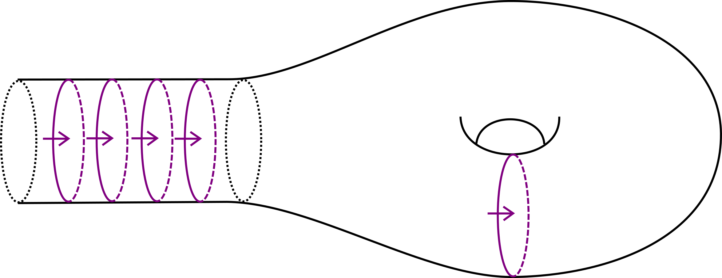
Let $g$ be the transverse map which is partially depicted in Figure 4.1, and $(\Sigma,f)$ be such that $\left[g\right]\in{\cal T}\left(\Sigma,f\right)$. The key feature of $g$ is that there is a null-curve (e.g., one of the dotted black lines) that separates a subsurface that is mapped by $f$ at the level of $\pi_{1}$ to the cyclic group $\langle x\rangle$. In terms of our picture, this can be seen as the curves that appear in this subsurface are associated to only one generator $x$. Note also in our picture we have illustrated a ‘neck’ region bounded by two black dotted curves that contains 4 parallel and codirected $(x,0)$-curves. Assume for the sake of clarity that any curve that could be drawn in the neck region is indeed drawn there. One could modify this transverse map by changing the number of the repeated curves in the neck region.

Lemma 4.16.

No matter how many parallel codirected $(x,0)$-curves are placed in the neck region of $g$, the resulting transverse map still realizes $(\Sigma,f)$ and thus represents an element of ${\cal T}\left(\Sigma,f\right)$.

?proofname?.

Call the rightmost $\left(x,0\right)$-arc in the neck $\alpha$ and the $\left(x,0\right)$-curve in the right part of Figure 4.1 $\beta$. Consider an $H$-move along a piece of arc connecting $\alpha$ to $\beta$ (and arrives to both from their positive side). This results in a strict transverse map in ${\cal T}\left(\Sigma,f\right)$ which is the same as $g$ except that $\alpha$ is omitted. This shows that alternating the number of $\left(x,0\right)$-curve in the neck in Figure 4.1 does not take us out of ${\cal T}\left(\Sigma,f\right)$. ∎

Corollary 4.17.

With ${\cal T}={\cal T}(\Sigma,f)$ as in Lemma 4.16, obtained from Figure 4.1, $\mathrm{MCG}(f)\backslash{\cal T}$ is not finite.

?proofname?.

We can create elements in ${\cal T}$ with an unbounded number of curves, and the number of curves is a $\mathrm{MCG}(f)$-invariant. ∎

This is not the most general version of this phenomenon: the neck could for example be replaced by a collection of disjoint annuli that cut from $\Sigma$ some subsurface with $\pi_{1}$ mapped by $f$ to a non-trivial cyclic subgroup of $\mathrm{\mathbf{F}}_{r}$. Our aim here is to give an illustrative example.

5 Further applications and consequences

We specify here three interesting applications of our results and techniques, regarding the stable commutator length of a word, the complete classification of all incompressible solutions in $\mathsf{Surfaces}\left(w_{1},\ldots,w_{\ell}\right)$, and the cohomological dimension of $\mathrm{MCG}\left(f\right)$. Let us also mention that our construction of a finite $K\left(\Gamma,1\right)$-space for $\Gamma=\mathrm{MCG}\left(f\right)$ when $\left[\left(\Sigma,f\right)\right]$ is incompressible also enables one to write explicit finite presentations for $\Gamma$: consult [MP15, Pages 57-59].

5.1 Stable commutator length

Recall that Corollary 1.11 states that the $w$-measures on $\left\{\mathcal{U}\left(n\right)\right\}_{n\in\mathbb{N}}$ determine $\mathrm{scl}\left(w\right)$, the stable commutator length of $w\in\mathrm{\mathbf{F}}_{r}$, defined in (1.7). In this subsection we explain how this result follows from Theorem 1.7 and from Calegari’s rationality theorem.

Calegari’s theorem, which is the main result of [Cal09b], says that $\mathrm{scl}\left(w\right)$ is rational for every $w\in\left[\mathrm{\mathbf{F}}_{r},\mathrm{\mathbf{F}}_{r}\right]$. First, it is shown that $\mathrm{scl\left(w\right)}$ is equal to the infimum of $\frac{-\chi\left(\Sigma\right)}{2\left|j_{1}+\ldots+j_{\ell}\right|}$ over all possible $j_{1},\ldots,j_{\ell}\in\mathbb{Z}$ and $\left(\Sigma,f\right)$ admissible for $w^{j_{1}},\ldots,w^{j_{\ell}}$ [Cal09b, Lemma 2.6]. The proof goes through showing the existence of “extremal surfaces” for $w$: a surface attaining the infimum. Moreover, by [Cal09b, Lemma 2.7], this extremal surface can be taken to be admissible for $w^{j_{1}},\ldots,w^{j_{\ell}}$ with $j_{1},\ldots,j_{\ell}>0$. By definition of extremal surface, $\Sigma$ has maximal Euler characteristic for $w^{j_{1}},\ldots,w^{j_{\ell}}$, namely, $\chi\left(\Sigma\right)=\chi_{\max}\left(w^{j_{1}},\ldots,w^{j_{\ell}}\right)$. In fact, every surface which is admissible for $w^{j_{1}},\ldots,w^{j_{\ell}}$ with Euler characteristic $\chi_{\max}\left(w^{j_{1}},\ldots,w^{j_{\ell}}\right)$ is extremal. By [Cal09b, Lemma 2.9], the maps associated with extremal surfaces are $\pi_{1}$-injective, namely, if $\gamma\subset\Sigma$ is a non-nullhomotopic closed curve, then $f\left(\gamma\right)$ is not nullhomotopic. Note that this condition is stronger than incompressibility, which only deals with simple closed curves. The crux of the matter is the following lemma:

Lemma 5.1.

If $\left(\Sigma,f\right)$ is $\pi_{1}$-injective, then $\mathrm{MCG}\left(f\right)$ is trivial.

?proofname?.

The outline of the argument here is that if $\left[\rho\right]\in\mathrm{MCG}\left(f\right)$ then $\left[\rho\right]_{*}\in\mathrm{Aut}\left(\pi_{1}\left(\Sigma\right)\right)$ fixes $f_{*}$, and since $f_{*}$ is injective, this means that $\left[\rho\right]_{*}$ must be the identity. By a variation of the Dehn-Nielsen-Baer Theorem, it follows that $\left[\rho\right]$ is the identity.

In more detail, assume that $\Sigma$ is connected (the general cases easily follows). Recall that $v_{1}\in\partial_{1}\Sigma$ is one of the $\ell$ marked points at $\partial\Sigma$, and let $G=\pi_{1}\left(\Sigma,v_{1}\right)$. If $\ell=1$, the Dehn-Nielsen-Baer Theorem (see Page 1 and [MP15, Thm 2.4]) yields what we need. If $\ell\geq 2$, consider an arc $\gamma\subset\Sigma$ connecting $v_{1}$ and $v_{\ell}$. Because $\left[\rho\right]\in\mathrm{MCG}\left(\Sigma\right)$ fixes the marked points, we must have that $\rho\left(\gamma\right)$ is homotopic relative to $\left\{v_{1},v_{\ell}\right\}$ to $\beta*\gamma$, where $\beta$ is a closed, not necessarily simple, curve based at $v_{1}$ and “$*$” stands for concatenation. Inside $\mathrm{\mathbf{F}}_{r}$ we have

$$f_{*}\left[\gamma\right]=f_{*}\left[\rho\left(\gamma\right)\right]=f_{*}\left[\beta*\gamma\right]=f_{*}\left[\beta\right]\cdot f_{*}\left[\gamma\right]$$

hence $f_{*}\left[\beta\right]=1$ which means that $\beta$ is nullhomotopic by $\pi_{1}$-injectivity. Hence we can assume without loss of generality that $\rho$ fixes $\gamma$, and we can analyze $\rho$ on $\Sigma^{\prime}$, the surface obtained from $\Sigma$ by cutting along $\gamma$. Since $\Sigma^{\prime}$ has only $\ell-1$ boundary components, we are done by induction. ∎

Proof of Corollary 1.11.

By Lemma 5.1 and the discussion preceding it, if one of the extremal surfaces of $w$ is admissible for $w^{j_{1}},\ldots,w^{j_{\ell}}$ with $j_{1},\ldots,j_{\ell}>0$, then Theorem 1.7 translates in this case to

$${\cal T}r_{w^{j_{1}},\ldots,w^{j_{\ell}}}\left(n\right)=n^{\chi_{\max}\left(w^{j_{1}},\ldots,w^{j_{\ell}}\right)}\cdot K+O\left(n^{\chi_{\max}\left(w^{j_{1}},\ldots,w^{j_{\ell}}\right)-2}\right),$$ (5.1)

where $K$ is the number of highest-Euler-characteristic surfaces in $\mathsf{Surfaces}\left(w^{j_{1}},\ldots,w^{j_{\ell}}\right)$. Note that (5.1) is strictly positive for large enough $n$. Hence,

$$\frac{-\lim_{n\to\infty}\log_{n}\left|{\cal T}r_{w^{j_{1}},\ldots,w^{j_{\ell}}}\left(n\right)\right|}{2\left(j_{1}+\ldots+j_{\ell}\right)}=\frac{-\chi_{\max}\left(w^{j_{1}},\ldots,w^{j_{\ell}}\right)}{2\left(j_{1}+\ldots+j_{\ell}\right)}=\mathrm{scl}\left(w\right).$$

On the other hand, for an arbitrary $\ell>0$ and $j_{1},\ldots,j_{\ell}>0$ we have

$$\frac{-\lim_{n\to\infty}\log_{n}\left|{\cal T}r_{w^{j_{1}},\ldots,w^{j_{\ell}}}\left(n\right)\right|}{2\left(j_{1}+\ldots+j_{\ell}\right)}\geq\frac{-\chi_{\max}\left(w^{j_{1}},\ldots,w^{j_{\ell}}\right)}{2\left(j_{1}+\ldots+j_{\ell}\right)}\geq\mathrm{scl}\left(w\right).$$

This proves (1.8). ∎

Corollary 5.2.

If $\mathrm{scl}\left(w_{1}\right)\neq\mathrm{scl}\left(w_{2}\right)$ then for every large enough $n$, the $w_{1}$-measure on ${\cal U}\left(n\right)$ is different from the $w_{2}$-measure on ${\cal U}\left(n\right)$. In particular, if $w_{1}\in\left[\mathrm{\mathbf{F}}_{r},\mathrm{\mathbf{F}}_{r}\right]$ and $w_{2}\notin\left[\mathrm{\mathbf{F}}_{r},\mathrm{\mathbf{F}}_{r}\right]$ then they induce different measures on ${\cal U}\left(n\right)$ for almost all $n$.

?proofname?.

Assume without loss of generality that $\mathrm{scl}\left(w_{1}\right)<\mathrm{scl}\left(w_{2}\right)$, and let $j_{1},\ldots,j_{\ell}>0$ be so that $w_{1}^{j_{1}},\ldots,w_{1}^{j_{\ell}}$ admit an extremal surface. Then by the above discussion, ${\cal T}r_{w_{1}^{j_{1}},\ldots,w_{1}^{j_{\ell}}}\left(n\right)$ is strictly larger than ${\cal T}r_{w_{2}^{j_{1}},\ldots,w_{2}^{j_{\ell}}}\left(n\right)$ for any large enough $n$. In particular, if $w_{2}$ is not balanced, i.e. $w_{2}\notin\left[\mathrm{\mathbf{F}}_{r},\mathrm{\mathbf{F}}_{r}\right]$ and $\mathrm{scl}\left(w_{2}\right)=\infty$, then nor is the set $w_{2}^{j_{1}},\ldots,w_{2}^{j_{\ell}}$ balanced as we assume $j_{1},\ldots,j_{\ell}>0$. By Claim 2.1, ${\cal T}r_{w_{2}^{j_{1}},\ldots,w_{2}^{j_{\ell}}}\left(n\right)\equiv 0$ for every $n$. ∎

5.2 Classifying all incompressible solutions to generalized commutator equation

Since the late 1970’s there are known algorithms to determine the commutator length of a given word $w\in\left[\mathrm{\mathbf{F}}_{r},\mathrm{\mathbf{F}}_{r}\right]$ [Edm75, GT79, Cul81] and also to find at least one representative from every equivalence class of solutions to $\left[u_{1},v_{1}\right]\cdots\left[u_{g},v_{g}\right]=w$ with $g={\cal\mathrm{cl}}\left(w\right)$ [Cul81, Section 4.2]. In fact, the algorithm in [Cul81] uses matchings of letters of $w$ as in Proposition 2.13. Our analysis and techniques expand Culler’s algorithm to yield a clear description of the set of classes of solutions and, in particular, a direct way to distinguish them from each other.

Consider the poset $P=\mathrm{\overline{MATCH}}^{\left|\kappa\right|\leq 1}\left(w_{1},\ldots,w_{\ell}\right)$ consisting of sets of matchings for $w_{1},\ldots,w_{\ell}$ as in Section 2, where $\left|\kappa\right|\stackrel{{\scriptstyle\mathrm{def}}}{{=}}\sum_{x\in B}\kappa_{x}\leq 1$ and $\sigma_{x,0}\neq\sigma_{x,1}$ whenever $\kappa_{x}=1$, and with partial order $\sigma_{0}\prec\sigma_{1}$ whenever $\left|\kappa\left(\sigma_{0}\right)\right|=0$, $\left|\kappa\left(\sigma_{1}\right)\right|=1$ and $\sigma_{0}$ is obtained from $\sigma_{1}$ by deleting one of the two $x$-matchings for the $x\in B$ with $\kappa_{x}\left(\sigma_{1}\right)=1$. Recall the definition of $\chi\left(\sigma\right)$ from Definition 2.7. Construct a graph $G\left(w_{1},\ldots,w_{\ell}\right)$ with vertices the elements of $P$ and an edge $\left(\sigma_{0},\sigma_{1}\right)$ whenever $\sigma_{0}\prec\sigma_{1}$ and $\chi\left(\sigma_{1}\right)=\chi\left(\sigma_{2}\right)$. We say a component $C$ of $G\left(w_{1},\ldots,w_{\ell}\right)$ is downward-closed if every vertex $\sigma_{1}$ of $C$ with $\kappa\left(\sigma_{1}\right)=1$ has two neighbors: the two elements of $P$ that are strictly smaller. Recall the notation $\Sigma_{\sigma}$ and $f_{\sigma}$ from Definitions 2.7 and 2.11.

Proposition 5.3.

The map $\varphi\colon P=\mathrm{\overline{MATCH}}^{\left|\kappa\right|\leq 1}\to\mathsf{Surfaces}\left(w_{1},\ldots,w_{\ell}\right)$ given by

$$\sigma\mapsto\left[\left(\Sigma_{\sigma},f_{\sigma}\right)\right]$$

induces a bijection between the downward-closed components of $G\left(w_{1},\ldots,w_{\ell}\right)$ and the incompressible pairs in $\mathsf{Surfaces}\left(w_{1},\ldots,w_{\ell}\right)$.

?proofname?.

First, $\varphi$ is constant on connected components of $G\left(w_{1},\ldots,w_{\ell}\right)$: indeed, assume that $\sigma_{0}\prec\sigma_{1}$ with $\chi\left(\sigma_{0}\right)=\chi\left(\sigma_{1}\right)$ and, say, $\sigma_{0}$ is obtained from $\sigma_{1}$ by forgetting the matching $\left(\sigma_{1}\right)_{x,1}$. Then the condition $\chi\left(\sigma_{0}\right)=\chi\left(\sigma_{1}\right)$ shows forgetting the $\left(x,1\right)$ transversion point of the transverse map $f_{\sigma_{1}}$ results in a transverse map which is still filling, and thus equal to $f_{\sigma_{0}}$. Hence we can define $\hat{\varphi}$ to be a map from the downward-closed components of $G\left(w_{1},\ldots,w_{\ell}\right)$ to $\mathsf{Surfaces}\left(w_{1},\ldots,w_{\ell}\right)$.

Second, the image of $\hat{\varphi}$ consists of incompressible elements. To see this, let $C$ be a downward-closed component of $P$. Let $\sigma\in C$ have $\left|\kappa\left(\sigma\right)\right|=0$. Assume to the contrary that $\varphi\left(\sigma\right)$ is compressible. Then it admits a null-curve $\gamma$ which is not disjoint from the matching-edges in $\Sigma_{\sigma}$ (recall that the matching-edges cut $\Sigma_{\sigma}$ to discs). One can start performing $H$-moves along this null-curve. In an $H$-move between two $x$-matching-edges $e_{1}$ and $e_{2}$ along a piece of $\gamma$, one first creates a transverse map $g_{1}$ with $\left|\kappa\left(g_{1}\right)\right|=1$ (with $f_{\sigma}\prec g_{1}$ in ${\cal T}={\cal T}\left(\Sigma_{\sigma},f_{\sigma}\right)$) and then obtains $g_{0}\prec_{{\cal T}}g_{1}$ with $\left|\kappa\left(g_{0}\right)\right|=0$ which has two fewer intersection points with $\gamma$. Because the matching-edges cut $\Sigma_{\sigma}$ to disks, $e_{1}$ and $e_{2}$ must be distinct, and thus $g_{1}$ has only arcs and $\left[g_{1}\right]=\left[f_{\sigma_{1}}\right]$ for some $\sigma_{1}\in C$. As $C$ is downward-closed, there is some $\sigma_{0}\in C$ with $\left[g_{0}\right]=\left[f_{\sigma_{0}}\right]$. We can continue in the same manner until $\gamma$ intersects no matching-edges, which is a contradiction.

Third, $\hat{\varphi}$ is the sought-after bijection. Indeed, every incompressible $\left[\left(\Sigma,f\right)\right]\in\mathsf{Surfaces}\left(w_{1},\ldots,w_{\ell}\right)$ is the $\varphi$-image of some component of $G\left(w_{1},\ldots,w_{\ell}\right)$ by Proposition 2.13. If $\sigma\in P$ satisfies $\varphi\left(\sigma\right)=\left[\left(\Sigma,f\right)\right]$ and $C$ is the connected component of $\sigma$ then $C$ is a component of the $1$-skeleton of the $K\left(\Gamma,1\right)$-complex we constructed in the proof of Theorem 1.6 in Section 4.4. In particular, this complex is connected (because its universal cover $\left|{\cal T}\right|_{\mathrm{poly}}$ is connected), hence so its $1$-skeleton is connected. This shows that $C$ is the only component mapping to $\left[\left(\Sigma_{\sigma},f_{\sigma}\right)\right]$ and that it is downward-closed. ∎

Alternatively, one could use here a direct argument imitating some ingredients from the proof of Theorem 3.14, as follows. For $\left[\left(\Sigma,f\right)\right]$ incompressible, show that $\varphi^{-1}\left(\left[\left(\Sigma,f\right)\right]\right)$ is a downward-closed connected component of $G\left(w_{1},\ldots,w_{\ell}\right)$, by taking a maximal system of null-arcs, showing there is a single $\sigma_{0}\in\varphi^{-1}\left(\left[\left(\Sigma,f\right)\right]\right)$ with matching edges disjoint from these null-arcs, and showing every other element in the preimage can be connected to $\sigma_{0}$ by $H$-moves that never leave the same connected component of $G\left(w_{1},\ldots,w_{\ell}\right)$.

5.3 Finiteness of the cohomological dimension of the stabilizer $\mathrm{MCG}\left(f\right)$

Recall that the cohomological dimension, $\mathrm{cd}(\Gamma)$, of a torsion-free group $\Gamma$ is the minimal length of a projective resolution of $\mathbf{\mathbf{Z}}$ over $\mathbf{\mathbf{Z}}\Gamma$ if one exists, and $\infty$ otherwise. If a group $\Gamma$ is virtually torsion-free then the virtual cohomological dimension, $\mathrm{vcd}(\Gamma)$, is defined to be $\mathrm{cd}(\Gamma^{\prime})$ where $\Gamma^{\prime}$ is a finite index torsion-free subgroup of $\Gamma$; it is a theorem of Serre [Ser71] that the resulting dimension does not depend on the chosen finite index subgroup. As the the following result is not needed for the main results of this paper, we only sketch its proof.

Proposition 5.4.

Let $\Sigma$ be a compact orientable surface with no closed connected components and let $f\colon\Sigma\to{\textstyle\bigvee^{r}S^{1}}$ be a map. Then $\mathrm{cd}(\mathrm{MCG}(f))<\infty$.

Sketch of proof.

Let ${\cal T}={\cal T}(\Sigma,f)$ and $\Gamma=\mathrm{MCG}(f)$. Note that $\Gamma$ is torsion-free since $\Sigma$ has no closed components. We use a result that is attributed to Quillen by Serre in [Ser71, Prop. 11(a)]. As $\left|{\cal T}\right|_{\mathrm{poly}}$ is contractible (Theorem 3.14), Quillen’s result says that

$$\mathrm{cd}(\Gamma)\leq\sup_{[g]\in\Gamma\backslash{\cal T}}\left(\dim(\mathrm{polysim}\left(\left[g\right]\right))+\mathrm{cd}(\mathrm{Stab}_{\Gamma}(g)\right).$$

Therefore, as $\left|{\cal T}\right|_{\mathrm{poly}}$ is finite dimensional (Lemma 3.12), it suffices to prove there is an upper bound depending only on the pair $(\Sigma,f)$ for $\mathrm{cd}(\mathrm{Stab}_{\Gamma}(g))$ given an arbitrary element $g$ in ${\cal T}$.

We now give a quick analysis of these stabilizers. Fix a transverse map $g$ with $\left[g\right]\in{\cal T}$. Let $\left\{\Sigma_{i}\right\}_{i\in I}$ denote the zones of $g$ which are not annuli bounded by two curves of $g$. By Euler characteristic argument, $I$ is finite and bounded independently of $g$. Form $\Sigma_{i}^{*}$ by contracting each end of $\Sigma_{i}$ bounded by a curve of $g$ to a point, and mark the new points $W_{i}\subset\Sigma_{i}^{*}$ on their respective surfaces. We denote by $\mathrm{MCG}(\Sigma_{i}^{*},W_{i})$ the mapping class group of $\Sigma_{i}^{*}$ that fixes each individual element of $W_{i}$.

The subgroup $\Gamma_{0}\leq\mathrm{Stab}_{\Gamma}\left(g\right)$ that fixes all the curves in $g$ and their orientations has finite index in $\mathrm{Stab}_{\Gamma}\left(g\right)$, and there is a short exact sequence obtained by restricting mapping classes in $\Gamma_{0}$ to the zones $\Sigma_{i}$:

$$1\to N\to\Gamma_{0}\to H\overset{\mathrm{def}}{=}\prod_{i\in I}\mathrm{MCG}(\Sigma_{i}^{*},W_{i})\to 1,$$ (5.2)

where $N$ is a free abelian group generated by Dehn twists in the curves of $g$. The reason one obtains the whole of each $\mathrm{MCG}(\Sigma_{i}^{*},W_{i})$ as a factor is because $g$ maps each $\Sigma_{i}$ to a contractible piece of ${\textstyle\bigvee^{r}S^{1}}$, and any lift of any element of $\mathrm{MCG}(\Sigma_{i}^{*},W_{i})$ to $\mathrm{MCG}(\Sigma)$ can be taken to be the identity outside $\Sigma_{i}$, and therefore preserves the homotopy class of $f$. Although $\mathrm{MCG}(\Sigma_{i}^{*},W_{i})$ could contain torsion, it is virtually torsion-free (see either [Iva02, Theorem 6.8.A] or [Har86, §4]).

Harer proved in [Har86] that for any surface $\Sigma$ and collection of interior marked points $W$,

$$\mathrm{vcd}(\mathrm{MCG}(\Sigma,W))\leq 4g(\Sigma)+2|\pi_{0}(\partial\Sigma)|+|W|-3,$$

where $g\left(\Sigma\right)$ is the genus of $\Sigma$. Therefore using [Bro82, Prop. VIII.2.4.b] together with an argument as in [Bro82, Proof of Prop. IX.7.3.d] to pass between $\mathrm{vcd}$ and $\mathrm{cd}$, one obtains

$$\mathrm{vcd}(H)\leq\sum_{i\in I}\left(4g(\Sigma_{i}^{*})+2|\pi_{0}(\partial\Sigma_{i}^{*})|+|W_{i}|-3\right)\leq F_{1}\left(\Sigma\right),$$

where $F_{1}\left(\Sigma\right)$ is a bound in terms of $\Sigma$ which is independent of $g$. Since $H$ is virtually torsion-free, and $\Gamma_{0}$ has no torsion, we can find torsion-free finite index subgroups $\Gamma^{\prime}_{0},H^{\prime}$ in $\Gamma_{0}$ and $H$ respectively that form a short exact sequence $1\to N\to\Gamma^{\prime}_{0}\to H^{\prime}\to 1$. Then Serre’s Theorem [Ser71] gives $\mathrm{cd}(\mathrm{Stab}_{\Gamma}(g))=\mathrm{cd}(\Gamma_{0})=\mathrm{cd}(\Gamma^{\prime}_{0})$ and $\mathrm{cd}(H^{\prime})=\mathrm{vcd}(H)$. We also have $\mathrm{cd}\left(N\right)\leq F_{2}(\Sigma)$ where $F_{2}(\Sigma)$ is the maximal number of pairwise non-isotopic disjoint simple closed curves on $\Sigma$. Now applying [Bro82, Prop. VIII.2.4.b] to the short exact sequence for $N,\Gamma_{0}^{\prime},H^{\prime}$ we get

$$\mathrm{cd}(\mathrm{Stab}_{\Gamma}(g))=\mathrm{cd}(\Gamma_{0}^{\prime})\leq\mathrm{cd}(N)+\mathrm{cd}(H^{\prime})=\mathrm{cd}(N)+\mathrm{vcd}(H)<F_{1}\left(\Sigma\right)+F_{2}\left(\Sigma\right).$$

∎

6 Open problems

We mention some open problems that naturally arise from the discussion in this paper.

1. Recall that primitive words are the orbit in $\mathrm{\mathbf{F}}_{r}$ of the single-letter word $x$ under the action of $\mathrm{Aut}\left(\mathrm{\mathbf{F}}_{r}\right)$. As mentioned on Page 1.10, it was shown in [PP15] that only primitive words induce uniform measure on the symmetric group $S_{n}$ for all n. Is the same true for unitary groups? Namely, if a word induces Haar measure on $\mathcal{U}\left(n\right)$ for all $n$, is the word necessarily primitive? In fact, the following question raised by Tsachik Gelander a few years ago (by private communication) is still open: if a word induces Haar measure on $\mathcal{U}\left(2\right)$, is the word necessarily primitive?

2. Fix $j_{1},\ldots,j_{\ell}\in\mathbb{Z}$. Given $w\in\mathrm{\mathbf{F}}_{r}$, is there a nice criterion for determining whether the rational expression for ${\cal T}r_{w^{j_{1}},\ldots,w^{j_{\ell}}}\left(n\right)$ has the same value as for the primitive case when $w=x$? An illustrating example is ${\cal T}r_{w}\left(n\right)$ – we know it vanishes outside $\left[\mathrm{\mathbf{F}}_{r},\mathrm{\mathbf{F}}_{r}\right]$, but it is not clear when it vanishes inside $\left[\mathrm{\mathbf{F}}_{r},\mathrm{\mathbf{F}}_{r}\right]$. Another illustrating example is ${\cal T}r_{w,w^{-1}}\left(n\right)$: when does it differ from $1$? Some examples for each are elaborated in Table 1 and on Page 1.

3. Let $\Sigma$ be a connected, orientable surface with boundary, and let $f\colon\Sigma\to{\textstyle\bigvee^{r}S^{1}}$. We showed here that $\mathrm{MCG}\left(f\right)$ has a well-defined $L^{2}$-Euler-characteristic (Theorem 1.4) and a finite cohomological dimension (Proposition 5.4). Does $\mathrm{MCG}\left(f\right)$ always have “finite homological type” as defined in [Bro82, Page 246]? And if so, does its ordinary Euler characteristic coincide with the $L^{2}$-one?

4. We deduced the rationality of ${\cal T}r_{w_{1},\ldots,w_{\ell}}\left(n\right)$ in Theorem 2.8 directly from Weingarten calculus. The rationality means that the different $L^{2}$-Euler characteristics appearing in Theorem 1.7 “know” about each other. Is it possible to deduce the rationality of ${\cal T}r_{w_{1},\ldots,w_{\ell}}\left(n\right)$ (i.e., Proposition 1.1) from our main theorem, Theorem 1.7?

5. What can one say about the distribution of ${\cal T}r_{w}\left(n\right)$ when $w$ is a long random word in $\left[\mathrm{\mathbf{F}}_{r},\mathrm{\mathbf{F}}_{r}\right]$? For example, what is the distribution of the commutator length of $w$? Is it true that for most words of a fixed length in $\left[\mathrm{\mathbf{F}}_{r},\mathrm{\mathbf{F}}_{r}\right]$, the stabilizers $\mathrm{MCG}\left(f\right)$ of incompressible solutions are trivial?

6. What can one systematically say about the $L^{2}$-Euler characteristic of $\mathrm{MCG}(f)$? For which $f$ are they zero, negative, or positive? The case when $f$ is incompressible is a natural starting point. A sufficiently good understanding of this question would allow one to make progress on Conjecture 1.10. The Euler characteristic of the mapping class group of a closed surface was calculated by Harer-Zagier [HZ86] and the sign of the Euler characteristic of the mapping class group was re-obtained by McMullen [McM00] by different methods.

Michael Magee,
Department of Mathematical Sciences,
Durham University,
Lower Mountjoy, DH1 3LE Durham,
United Kingdom

michael.r.magee@durham.ac.uk

Doron Puder,
School of Mathematical Sciences,
Tel Aviv University,
Tel Aviv, 6997801, Israel
doronpuder@gmail.com