Adapting the CVA model to Leland’s framework

Abstract

We consider the framework proposed by Burgard and Kjaer in [1] that derives the PDE which governs the price of an option including bilateral counterparty risk and funding. We extend this work by relaxing the assumption of absence of transaction costs in the hedging portfolio by proposing a cost proportional to the amount of assets traded and the traded price. After deriving the nonlinear PDE, we prove the existence of a solution for the corresponding initial-boundary value problem. Moreover, we develop a numerical scheme that allows to find the solution of the PDE by setting different values for each parameter of the model. To understand the impact of each variable within the model, we analyze the Greeks of the option and the sensitivity of the price to changes in all the risk factors.

Keywords: Nonlinear parabolic differential equations, Option pricing models, Transaction costs, CVA, Euler method.

2010 MSC: 35K20, 35K55, 91G20, 91G60.

1 Introduction

Under the Black-Scholes pricing framework [2], the price of an option is derived by constructing a hedging portfolio consisting of a certain amount of the underlying asset and a money-market account. This methodology relies on a list of different assumptions that are set to simplify the model. For example, constant values of volatility and interest rates, the non-existence of dividend yields, the efficiency of the markets and the non-existence of transaction costs, among others. Nonetheless, the probability of default of both the issuer of the option and the counterparty are not being considered when constructing the hedging portfolio. Therefore, it is expected that the option price obtained by the standard modeling approach will be different when compared with the actual price of the contract.

As explained in [3], the counterparty credit risk is the risk that a counterparty in a financial contract defaults prior to the expiration of the contract and fails to make future payments. To include this probability in the pricing of a contract, the Credit Valuation Adjustment (CVA) is used. As described in [4], CVA is defined as the difference between the price of the instrument including credit risk and the price where the counterparty of the transaction is considered free of risk. By definition, the CVA will be always positive if only the counterparty risk is considered. When the issuer credit riskiness is also taken into account, the Debit Valuation Adjustment (DVA) is included into the formula. The DVA acts oppositely as the CVA by adding value to the option when the issuer risk increases. If we set $V_{BS}$ as the Black-Scholes option price default free and $V$ as the adjusted option price we get

$$V\,=\,V_{BS}\,-\,CVA\,+\,DVA$$

where $CVA$ is a cost and $DVA$ is a benefit.

As mentioned in [4], before 2008 crisis, CVA was commonly calculated and charged only by tier one banks by choosing either unilateral or bilateral models. After 2008 crisis, not only bilateral CVA started to be widely used but also a different set of value adjustments began to be applied such as the Funding Valuation Adjustment or FVA (including costs of of funding) and the Capital Valuation Adjustment or KVA (including cost of capital).

Several works have been developed within the family of value adjustments for different OTC derivatives. In [5], the authors derive the CVA by decomposing the portfolio’s value into a set of binary states: positive or negative cash flows directions, two possible default states and to receive or not the recovery rate. In [6], the authors study a CDS pricing model which includes the probability of default of the counterparty. Credit spread volatilities are considered by assuming default intensities following a CIR dynamic with a correlation parameter within. The authors in [7] generalize these model in two ways. First, by allowing correlation not only between default times but also with the underlying portfolio risk factors (interest rates). Second, by considering the probability of default of the issuer.

These previous works are then expanded by [8] in order to apply that methodology on IR Swaps and IR Exotics. DVA and FVA are included in the pricing framework by [9] where a recursive formula is obtained after discounting all the cash flows occurring after the trading position is entered. These cash flows include not only the product cash flows (coupons, dividends, etc) but also cash flows required by collateral margining, funding and investing procedures and default events.

Finally, two works try to propose a general theory. In [1] the authors analyze the bilateral counterparty risk (CVA and DVA) with funding costs (FVA) by constructing a hedging portfolio composed by the underlying asset, a risk-free zero-coupon bond and two default risky zero-coupon bond of both the issuer and the counterparty. A PDE is formalized by applying the standard self-financing assumption. In [10] (and further in [11, 12]), the author applies a risk-neutral pricing approach under funding constraints in order to obtain a reduced-form backward stochastic differential equation (BSDE) approach to the problem of hedging and pricing the CVA.

The second assumption covered in our model is the (non) existence of transaction costs. Following Leland’s approach [13], transaction costs can be included in the pricing methodology by applying a discrete-time replicating strategy. A nonlinear partial differential equation is obtained for the option price , which is denoted by $V\left(S,t\right)$; namely,

$$\frac{\partial V}{\partial t}+\frac{1}{2}\hat{\sigma}\left(S\frac{\partial^{2}V}{\partial S^{2}}\right)^{2}S^{2}\frac{\partial^{2}V}{\partial S^{2}}+rS\frac{\partial V}{\partial S}-rV=0,$$

where $\hat{\sigma}$ is defined based upon the transaction costs function. This approach was then continued and improved by [14] and [15].

Different choices of transaction costs functions lead to variations on the nonlinear term of the partial differential equation. In [16], the authors propose a non-increasing linear function and find solutions for the stationary problem. In [17], the concept of transaction costs function is generalized and the so-called mean value modification of the transaction costs function is developed. This transformation allows the authors to formulate a general one-dimensional Black-Scholes equation by solving the equivalent quasilinear Gamma equation. Other authors [18, 19] also find solutions to the problem with constant transaction costs and relaxing the assumptions of constant volatility and interest rate.

The main distinctive aspect in the above-cited works is that they all consider only one asset within the partial differential equation. In [20] and [21], the author generalizes the Leland approach to cover different types of multi-asset options, developing the nonlinear partial differential equation and solving numerically a list of examples. In [22] the authors combine a multidimensional approach with a general transaction cost function to derive a the dynamics of the option price under a fully nonlinear PDE.

In this work we adapt the work of Burgard and Kjaer [1] in order to include the transaction costs generated by trading the underlying assets and both the issuer and counterparty bonds. We propose an initial constant transaction cost function proportional to the amount of assets traded. As a consequence, we derive a nonlinear PDE that extends the results found in [1] and prove the existence of a solution by applying the Schauder Fixed-Point theorem. In the second part of the work, we develop a numerical approach to solve the PDE by considering a non-uniform grid on the spatial variable. The main greeks of the option (Delta, Gamma, Rho and Vega) are calculated and analyzed to understand how both the value adjustments and transaction costs affect the behavior of the option price. Nonetheless, a sensitivity analysis on the remaining parameters (hazard rate, recovery rates, etc) is performed to complete the study of the option price dynamics.

The structure of the paper is as follows. In Section 2 we propose the market model that leads to the nonlinear dynamic of the option price. In Section 3 we apply the Schauder Fixed-Point theorem to derive the existence of solution for the original problem. Finally, in Section 4, the numerical framework is developed and different results are obtained to understand how the parameters affect the option price.

2 Market Model

The original paper of [1] derives the PDE for the value of a financial derivative considering bilateral counterparty risk and funding costs. For this purpose they propose an economy consisting of a risk-free zero-coupon bond, two default risky zero-coupon bond with zero recovery of parties B and C and a spot asset with no default risk. B will refer to the seller and C to the counterparty. Notation will be followed from the original work [1].

The dynamics of the four tradable assets under the historical probability measure are defined as follows:

$$\begin{cases}dP_{R}&=P_{R}\,r\,dt,\\ dP_{B}&=P_{B}\,r_{B}\,dt\,-\,P_{B}\,dJ_{B},\\ dP_{C}&=P_{C}\,r_{C}\,dt\,-\,P_{C}\,dJ_{C},\\ dS&=\mu\,S\,dt\,+\,S\,dW_{t}.\end{cases}$$

The default risky zero-coupon bonds are modeled by considering both $r_{B}$ and $r_{C}$ interest rates and $J_{B}$ and $J_{C}$ the two independent point processes that jump from $0$ to $1$ on default of B and C respectively. The default risk-free zero-coupon bond is a deterministic process with drift equal to $r$ and the spot asset is modeled following a geometric brownian motion with drift $\mu$ and volatility $\sigma$. Throughout this work the parameters $r,r_{B},r_{C},\mu$ and $\sigma$ are positive and constant. Also we will use the following notation:

$$x^{+}\, =\,\max\left(x,0\right)$$

$$x^{-}\, =\,\min\left(x,0\right).$$

To derive the price of option $\hat{V}$, we adapt the standard Black-Scholes framework [2] applied in [1] by considering the Leland’s approach [13]. Hence, we create a self-financing portfolio covering all the underlying risk factors that hedges the option. Let $\Pi\left(t\right)$ be the seller’s portfolio which consists of $\delta\left(t\right)$ units of $S\left(t\right)$, $\alpha_{B}\left(t\right)$ units of $P_{B}\left(t\right)$, $\alpha_{C}\left(t\right)$ units of $P_{C}\left(t\right)$ and $\beta\left(t\right)$ units of cash. For hedging purposes we set $\Pi\left(t\right)+\hat{V}\left(t\right)=0$ and

$$-\hat{V}\left(t\right)=\Pi\left(t\right)=\delta\left(t\right)\,S\left(t\right)\,+\,\alpha_{B}\left(t\right)\,P_{B}\left(t\right)\,+\,\alpha_{C}\left(t\right)\,P_{C}\left(t\right)\,+\,\beta\left(t\right).$$ (1)

We define the transaction costs function for both default risky bonds $P_{B}$ and $P_{C}$ and the spot asset $S$ as follows:

$$\begin{cases}TC_{B}\left(t,P_{B}\right)&=C_{B}\,|\alpha_{B}\left(t\right)|\,P_{B}\left(t\right),\\ TC_{C}\left(t,P_{C}\right)&=C_{C}\,|\alpha_{C}\left(t\right)|\,P_{C}\left(t\right),\\ TC_{S}\left(t,S\right)&=C_{S}\,|\delta\left(t\right)|\,S\left(t\right)\end{cases}$$

where $C_{B},C_{C}$ and $C_{S}$ are positive constants. This definition of transaction costs is the standard approach applied initially in [13] and is the initial step to creating more complex dynamics. In this case, the costs are defined to be proportional to the amount of assets traded multiplied by the price of each asset. For the purpose of enhancing clarity, we drop the dependencies on every function.

By forcing the portfolio to be self-financing, we find that

$$-d\hat{V}=\delta\,dS\,+\,\alpha_{B}\,dP_{B}\,+\,\alpha_{C}\,dP_{C}\,+\,d\beta.$$ (2)

where $d\beta$ is decomposed as $d\beta=d\beta_{S}+d\beta_{F}+d\beta_{C}$ corresponding to the variations in the cash position due to each of the three assets. In this step we consider the effect of the transaction cost in the hedging strategy. On each time step, there would be a decrease in the cash account because of the cost of buying or selling a different amount of assets. Hence, the original calculations of [1] are modified as follows:

• The share position provides a dividend income, a financing cost and a transaction cost. The variation in the position is found to be

  $$d\beta_{S}=\delta\,\gamma_{S}\,S\,dt-\delta\,q_{S}\,S\,dt-dTC_{S}$$ (3)

• After the own bonds are purchased, if any surplus in cash is available, it must earn the free-risk-rate $r$. If borrowing money, the seller needs to pay the rate $r_{F}$. In this case, transaction costs appear when calculating the surplus after the own bonds purchasing. The variation in this position is determined by

  $$d\beta_{F} =r\,\left(-\hat{V}-\alpha_{B}\,P_{B}-TC_{B}\right)^{+}\,dt+r_{F}\left(-\hat{V}-\alpha_{B}\,P_{B}-TC_{B}\right)^{-}\,dt$$

  $$=r\,\left(-\hat{V}-\alpha_{B}\,P_{B}-TC_{B}\right)\,dt+s_{F}\left(-\hat{V}-\alpha_{B}\,P_{B}-TC_{B}\right)^{-}\,dt$$ (4)

  where $s_{F}=r_{F}-r$ is the funding spread.
  

• Finally, a financing cost due to short-selling the counterparty bond and its related transaction costs are considered for calculating the variation in the cash counterparty position as follows:

  $$d\beta_{C}=-\alpha_{C}\,r\,P_{C}\,dt-dTC_{C}.$$ (5)

By applying equations (3), (4) and (5) in (2), we obtain

$$-d\hat{V} =\delta\,dS+\alpha_{B}\,P_{B}\left(r_{B}\,dt-dJ_{B}\right)+\alpha_{C}\,P_{C}\left(r_{C}\,dt-dJ_{C}\right)-dTC_{C}-dTC_{S}\,+$$ (6)

$$\left[\,\left(-\hat{V}-\alpha_{B}\,P_{B}-TC_{B}\right)^{+}+r_{F}\left(-\hat{V}-\alpha_{B}\,P_{B}-TC_{B}\right)^{-}+\delta\left(\gamma_{S}-q_{S}\right)\,S-\alpha_{C}\,r\,P_{C}\ \right]dt$$

$$=\left[-r\hat{V}+s_{F}\left(-\hat{V}-\alpha_{B}\,P_{B}-TC_{B}\right)^{-}+\left(r_{B}-r\right)\alpha_{B}\,P_{B}+\left(r_{C}-r\right)\alpha_{C}\,P_{C}-r\,TC_{B}+\delta\,\left(\gamma_{S}-q_{S}\right)\right]dt$$

$$-dTC_{S}-dTC_{C}+\delta\,dS-\alpha_{B}\,P_{B}\,dJ_{B}-\alpha_{C}\,P_{C}\,dJ_{C}.$$ (7)

Also, the Ito lemma adapted for jump processes provides another equivalent calculation of the variation of the process $\hat{V}$:

$$d\hat{V}=\frac{\partial\hat{V}}{\partial t}\,dt+\frac{\partial\hat{V}}{\partial S}\,dS+\frac{1}{2}\sigma^{2}S^{2}\frac{\partial^{2}\hat{V}}{\partial S^{2}}\,dt+\bigtriangleup\hat{V}_{B}\,dJ_{B}+\bigtriangleup\hat{V}_{C}\,dJ_{C}$$ (8)

where $\bigtriangleup\hat{V}_{B}$ and $\bigtriangleup\hat{V}_{C}$ are calculated based on default conditions. In [1] it is showed that

$$\bigtriangleup\hat{V}_{B} =\hat{V}\left(t,S,1,0\right)-\hat{V}\left(t,S,0,0\right)=-\hat{V}+\hat{V}^{+}+\,R_{B}\,\hat{V}^{-}$$

$$\bigtriangleup\hat{V}_{C} =\hat{V}\left(t,S,0,1\right)-\hat{V}\left(t,S,0,0\right)=-\hat{V}+R_{C}\,\hat{V}^{+}+\,\hat{V}^{-}$$

Hence, by adding (7) and (8), and in order to hedge the risks related to the corporate bonds and the spot asset we find that

$$\delta =-\frac{\partial\hat{V}}{\partial S}$$

$$\alpha_{B} =\frac{-\hat{V}+\hat{V}^{+}+\,R_{B}\,\hat{V}^{-}}{P_{B}}$$

$$\alpha_{C} =\frac{-\hat{V}+R_{C}\,\hat{V}^{+}+\,\hat{V}^{-}}{P_{C}}$$

and

$$0= \left[-r\hat{V}+s_{F}\left(-\hat{V}-\alpha_{B}\,P_{B}-TC_{B}\right)^{-}+\left(r_{B}-r\right)\alpha_{B}\,P_{B}+\left(r_{C}-r\right)\alpha_{C}\,P_{C}-r\,TC_{B}+\delta\,S\,\left(\gamma_{S}-q_{S}\right)+\right.$$

$$\left.\frac{\partial\hat{V}}{\partial t}+\frac{1}{2}\sigma^{2}S^{2}\frac{\partial^{2}\hat{V}}{\partial S^{2}}\right]\,dt-dTC_{S}-dTC_{C}$$ (9)

By recalling the definition of the transaction costs, we can compute $dTC_{S}$ and $dTC_{C}$. Then, for the calculation of the transaction costs of the spot asset, we recall the value of $\delta$ and note that

$$dTC_{S}=C_{S}\,\lvert d\delta\rvert\,S\,\sim C_{S}\,\left\lvert\frac{\partial^{2}\hat{V}}{\partial S^{2}}\right\rvert\,\sigma\,S^{2}\sqrt{dt}\,\sqrt{\frac{2}{\pi}}$$ (10)

where the approximation is made by taking the expected value of $\lvert d\delta\rvert$ and the lowest order $\mathcal{O}\left(\sqrt{\Delta t}\right)$ as follows

$$E\left(\left\lvert d\delta\right\rvert\right)=E\left(\,\left\lvert\frac{\partial^{2}\hat{V}}{\partial S^{2}}\right\rvert\,dS\right)=\left\lvert\frac{\partial^{2}\hat{V}}{\partial S^{2}}\right\rvert\sigma\,S\,\sqrt{dt}\,E\left[\Phi\right]$$

and setting $\Phi$ as a standard normal random variable.

The variation of the transaction costs of the counterparty bond position is computed by applying the same rationale as before but over $\lvert d\alpha_{C}\rvert$ in this case. Then,

$$dTC_{C}=C_{C}\,\lvert d\alpha_{C}\rvert\,P_{C}\,\sim C_{C}\,\left\lvert R_{C}\,\frac{\partial\hat{V}}{\partial S}^{+}+\frac{\partial\hat{V}}{\partial S}^{-}-\frac{\partial\hat{V}}{\partial S}\right\rvert\,\sigma\,S\sqrt{dt}\,\sqrt{\frac{2}{\pi}}$$ (11)

where in this occasion the approximation is obtained by taking the expected value of $\lvert d\alpha_{C}\rvert$ as follows

$$E\left(\left\lvert d\alpha_{C}\right\rvert\right)=E\left(\,\,\left\lvert R_{C}\,\frac{\partial\hat{V}}{\partial S}^{+}+\frac{\partial\hat{V}}{\partial S}^{-}-\frac{\partial\hat{V}}{\partial S}\right\rvert\,dS\right)=\left\lvert R_{C}\,\frac{\partial\hat{V}}{\partial S}^{+}+\frac{\partial\hat{V}}{\partial S}^{-}-\frac{\partial\hat{V}}{\partial S}\right\rvert\sigma\,S\,\sqrt{dt}\,E\left[\Phi\right]$$

and setting again $\Phi$ as a standard normal random variable.

By recalling (10) and (11) and applying those computations in (9), we obtain the following nonlinear parabolic partial derivative equation

$$0= \left[-r\hat{V}+s_{F}\left(-\hat{V}-\alpha_{B}\,P_{B}-TC_{B}\right)^{-}+\left(r_{B}-r\right)\alpha_{B}\,P_{B}+\left(r_{C}-r\right)\alpha_{C}\,P_{C}-r\,TC_{B}+\delta\,S\,\left(\gamma_{S}-q_{S}\right)+\right.$$

$$\left.\frac{\partial\hat{V}}{\partial t}+\frac{1}{2}\sigma^{2}S^{2}\frac{\partial^{2}\hat{V}}{\partial S^{2}}\right]\,dt-C_{S}\,\left\lvert\frac{\partial^{2}\hat{V}}{\partial S^{2}}\right\rvert\,\sigma\,S^{2}\sqrt{dt}\,\sqrt{\frac{2}{\pi}}-C_{C}\,\left\lvert R_{C}\,\frac{\partial\hat{V}}{\partial S}^{+}+\frac{\partial\hat{V}}{\partial S}^{-}-\frac{\partial\hat{V}}{\partial S}\right\rvert\,\sigma\,S\sqrt{dt}\,\sqrt{\frac{2}{\pi}}$$

$$= \left[-r\hat{V}+s_{F}\left(-\hat{V}-\alpha_{B}\,P_{B}-C_{B}\,\left\lvert-\hat{V}+\hat{V}^{+}+\,R_{B}\,\hat{V}^{-}\right\rvert\right)^{-}+\left(r_{B}-r\right)\alpha_{B}\,P_{B}+\left(r_{C}-r\right)\alpha_{C}\,P_{C}\right.$$

$$\left.-r\,\left(C_{B}\,\left\lvert-\hat{V}+\hat{V}^{+}+\,R_{B}\,\hat{V}^{-}\right\rvert\right)-\frac{\partial\hat{V}}{\partial S}\,S\,\left(\gamma_{S}-q_{S}\right)+\frac{\partial\hat{V}}{\partial t}+\frac{1}{2}\sigma^{2}S^{2}\frac{\partial^{2}\hat{V}}{\partial S^{2}}\right]\,dt-C_{S}\,\left\lvert\frac{\partial^{2}\hat{V}}{\partial S^{2}}\right\rvert\,\sigma\,S^{2}\sqrt{dt}\,\sqrt{\frac{2}{\pi}}$$

$$-C_{C}\,\left\lvert R_{C}\,\frac{\partial\hat{V}}{\partial S}^{+}+\frac{\partial\hat{V}}{\partial S}^{-}-\frac{\partial\hat{V}}{\partial S}\right\rvert\,\sigma\,S\sqrt{dt}\,\sqrt{\frac{2}{\pi}}$$ (12)

By setting $\lambda_{B}=r_{B}-r$, $\lambda_{C}=r_{C}-r$ and applying the definitions of $\alpha_{B}$ and $\alpha_{C}$, (12) becomes

$$0= \left[-r\hat{V}+s_{F}\left(-\hat{V}^{+}-\,R_{B}\,\hat{V}^{-}-C_{B}\,\left\lvert-\hat{V}+\hat{V}^{+}+\,R_{B}\,\hat{V}^{-}\right\rvert\right)^{-}+\lambda_{B}\left(-\hat{V}+\hat{V}^{+}+\,R_{B}\,\hat{V}^{-}\right)\right.$$

$$+ \left.\lambda_{C}\left(-\hat{V}+R_{C}\,\hat{V}^{+}+\,\hat{V}^{-}\right)-r\,\left(C_{B}\,\left\lvert-\hat{V}+\hat{V}^{+}+\,R_{B}\,\hat{V}^{-}\right\rvert\,\right)-\frac{\partial\hat{V}}{\partial S}\,S\,\left(\gamma_{S}-q_{S}\right)+\frac{\partial\hat{V}}{\partial t}+\frac{1}{2}\sigma^{2}S^{2}\frac{\partial^{2}\hat{V}}{\partial S^{2}}\right]\,dt$$

$$- C_{S}\,\left\lvert\frac{\partial^{2}\hat{V}}{\partial S^{2}}\right\rvert\,\sigma\,S^{2}\sqrt{dt}\,\sqrt{\frac{2}{\pi}}-C_{C}\,\left\lvert R_{C}\,\frac{\partial\hat{V}}{\partial S}^{+}+\frac{\partial\hat{V}}{\partial S}^{-}-\frac{\partial\hat{V}}{\partial S}\right\rvert\,\sigma\,S\sqrt{dt}\,\sqrt{\frac{2}{\pi}}$$ (13)

The absolute value that involves the transaction costs due to the own bonds purchase can be reduced by noting that when $\hat{V}\geq 0$, its value is $0$ and when $\hat{V}<0$ it is equal to $\left(R_{B}-1\right)\,\hat{V}$. Hence,

$$\left\lvert-\hat{V}+\hat{V}^{+}+\,R_{B}\,\hat{V}^{-}\right\rvert=\left(R_{B}-1\right)\,\hat{V}^{-}$$

Using this reduction in (13), we get:

$$\left(-\hat{V}^{+}-\,R_{B}\,\hat{V}^{-}-C_{B}\,\left\lvert-\hat{V}+\hat{V}^{+}+\,R_{B}\,\hat{V}^{-}\right\rvert\right)^{-} =\left(-\hat{V}^{+}-\,R_{B}\,\hat{V}^{-}-C_{B}\,\left(R_{B}-1\right)\,\hat{V}^{-}\right)^{-}$$

$$=\left(-\hat{V}^{+}-\hat{V}^{-}\left[R_{B}-C_{B}\,\left(R_{B}-1\right)\right]\right)^{-}$$

$$=\begin{cases}-\hat{V}\quad\text{if}\quad\hat{V}\geq 0\\ \quad 0\quad\text{if}\quad\hat{V}<0\\ \end{cases}$$

$$=\,-\hat{V}^{+}.$$ (14)

Thus, by implementing (14) in (13),

$$0= -r\hat{V}-s_{F}\,\hat{V}^{+}+\lambda_{B}\left(-\hat{V}+\hat{V}^{+}+\,R_{B}\,\hat{V}^{-}\right)+\lambda_{C}\left(-\hat{V}+R_{C}\,\hat{V}^{+}+\,\hat{V}^{-}\right)-r\,C_{B}\,\left(R_{B}-1\right)\,\hat{V}^{-}$$

$$- \frac{\partial\hat{V}}{\partial S}\,S\,\left(\gamma_{S}-q_{S}\right)+\frac{\partial\hat{V}}{\partial t}+\frac{1}{2}\sigma^{2}S^{2}\frac{\partial^{2}\hat{V}}{\partial S^{2}}-\sigma\,S^{2}\,\sqrt{\frac{2}{\pi\,dt}}\left(C_{S}\,\left\lvert\frac{\partial^{2}\hat{V}}{\partial S^{2}}\right\rvert\,+S^{-1}\,C_{C}\,\left\lvert R_{C}\,\frac{\partial\hat{V}}{\partial S}^{+}+\frac{\partial\hat{V}}{\partial S}^{-}-\frac{\partial\hat{V}}{\partial S}\right\rvert\,\right).$$ (15)

If we introduce the parabolic operator $\mathcal{A}_{t}$ as

$$\mathcal{A}_{t}\equiv\frac{1}{2}\sigma^{2}S^{2}\frac{\partial^{2}\hat{V}}{\partial S^{2}}+\frac{\partial\hat{V}}{\partial S}\,S\,\left(q_{S}-\gamma_{S}\right)$$

then it follows that $\hat{V}$ is the solution of

$$0= \,\frac{\partial\hat{V}}{\partial t}+\mathcal{A}_{t}\hat{V}-\left(\lambda_{B}+\lambda_{C}+r\right)\,\hat{V}+\left(\lambda_{B}+\lambda_{C}\,R_{C}-s_{F}\right)\,\hat{V}^{+}+\left(\lambda_{B}\,R_{B}+\lambda_{C}-r\,\left(R_{B}-1\right)\,C_{B}\right)\,\hat{V}^{-}$$

$$- \,\sigma\,S^{2}\,\sqrt{\frac{2}{\pi\,dt}}\left(C_{S}\,\left\lvert\frac{\partial^{2}\hat{V}}{\partial S^{2}}\right\rvert\,+S^{-1}\,C_{C}\,\left\lvert R_{C}\,\frac{\partial\hat{V}}{\partial S}^{+}+\frac{\partial\hat{V}}{\partial S}^{-}-\frac{\partial\hat{V}}{\partial S}\right\rvert\,\right)$$ (16)

Looking forward to compare (16) with equation 26 from [1], we rearrange the terms that involve $\hat{V}$, $\hat{V}^{+}$ and $\hat{V}^{-}$ and obtain the following nonlinear parabolic PDE

$$\frac{\partial\hat{V}}{\partial t}+\mathcal{A}_{t}\hat{V}-r\,\hat{V}= \,s_{F}\,\hat{V}^{+}+\lambda_{C}\,\left(1-R_{C}\right)\,\hat{V}^{+}+\lambda_{B}\,\left(1-R_{B}\right)\,\hat{V}^{-}-r\,\left(1-R_{B}\right)\,C_{B}\,\hat{V}^{-}$$

$$+ \,\sigma\,S^{2}\,\sqrt{\frac{2}{\pi\,dt}}C_{S}\,\left\lvert\frac{\partial^{2}\hat{V}}{\partial S^{2}}\right\rvert\,+\sigma\,S\,\sqrt{\frac{2}{\pi\,dt}}C_{C}\,\left\lvert R_{C}\,\frac{\partial\hat{V}}{\partial S}^{+}+\frac{\partial\hat{V}}{\partial S}^{-}-\frac{\partial\hat{V}}{\partial S}\right\rvert.$$ (17)

The first three terms on the right hand side of (17) are equal to the nonlinear terms of the original model. The inclusion of the transaction costs in the hedging strategy brings to the model three new terms:

• The fourth term in the right hand side of (17) corresponds to the amount of cash that is not invested at $r$ rate when considering the surplus held by the seller after the purchase of its own bonds as it is shown in (4).
  

• The fifth term is the effect of the transaction costs due to buying or selling $\delta$ assets of $S$. It shall be noted that the term is equal to the corresponding one in Leland’s standard approach.
  

• The sixth term is the effect of the transaction costs due to shorting the counterparty bond.

Comparing (16) with Leland’s notation, we can define the modified volatility as

$$\hat{\sigma}^{2}=\sigma^{2}\,\left(1-\sqrt{\frac{2}{\pi\,dt}}\,\frac{C_{S}}{\sigma}\,\text{sgn}\left(\frac{\partial^{2}\hat{V}}{\partial S^{2}}\right)\right)$$ (18)

and noting that

$$\left\lvert R_{C}\,\frac{\partial\hat{V}}{\partial S}^{+}+\frac{\partial\hat{V}}{\partial S}^{-}-\frac{\partial\hat{V}}{\partial S}\right\rvert =\begin{cases}\left\lvert\left(1-R_{C}\right)\,\frac{\partial\hat{V}}{\partial S}\right\rvert\quad&\text{if}\quad\hat{V}\geq 0\\ \quad 0\quad&\text{if}\quad\hat{V}<0\\ \end{cases}$$

$$=\,\left(1-R_{C}\right)\,\left\lvert\,\frac{\partial\hat{V}}{\partial S}^{+}\right\rvert$$ (19)

we obtain the following differential equation

$$\frac{\partial\hat{V}}{\partial t}+\frac{1}{2}\,\hat{\sigma}^{2}\,S^{2}\,\frac{\partial^{2}\hat{V}}{\partial S^{2}}+\frac{\partial\hat{V}}{\partial S}\,S\,\left(q_{S}-\gamma_{S}\right)-r\,\hat{V}= \,s_{F}\,\hat{V}^{+}+\lambda_{C}\,\left(1-R_{C}\right)\,\hat{V}^{+}+\lambda_{B}\,\left(1-R_{B}\right)\,\hat{V}^{-}-r\,\left(1-R_{B}\right)\,C_{B}\,\hat{V}^{-}$$

$$+ \sigma\,S\,\sqrt{\frac{2}{\pi\,dt}}C_{C}\,\left(1-R_{C}\right)\,\left\lvert\,\frac{\partial\hat{V}}{\partial S}^{+}\right\rvert$$ (20)

Remark 2.1.

The left-hand side of equation (20) is effectively a Black-Scholes operator with a volatility parameter $\hat{\sigma}$, a dividend yield $\gamma_{S}$ and a financing cost (different to the risk-free interest rate) $q_{S}$. The right-hand side of the equation contains the nonlinear terms that arises from considering the existence of transaction costs and default risk. The inclusion of these ’extra’ costs can be thought as a perturbation to the original model. By assessing the magnitude of the parameters of each term, it can be noted that they are indeed small. Hazard rates, recovery rates and interest rates are always below $1$ and the transaction costs per unit of asset can be modeled between $0.025$ to $0.04$ as it is done in [13].

3 Existence

3.1 Preliminaries

For the purpose of finding the unique solution of the CVA problem with transaction costs, we set the mathematical framework in which we will work. Let $\Omega=\left(S_{min},S_{max}\right)$ be an open subset of $\mathbb{R}^{+}$ and $\Omega_{T}\,=\,\Omega\times\left(0,T\right)$. Let $1\leq p\leq\infty$ and $k\,\in\,\mathbb{N}$. We define the following Sobolev spaces

$$W^{k}_{p}\left(\Omega\right)\, =\,\left\{u\,\in\,L^{p}\left(\Omega\right)\,|D^{\alpha}u\,\in\,L^{p}\left(\Omega\right),1\leq\left\lvert\alpha\right\rvert\leq k\right\},$$

$$W^{2k,k}_{p}\left(\Omega_{T}\right)\, =\,\left\{u\,\in\,L^{p}\left(\Omega_{T}\right)\,|D^{\alpha}\partial_{t}^{\beta}u\,\in\,L^{p}\left(\Omega_{T}\right),1\leq\left\lvert\alpha\right\rvert+2\beta\leq 2k\right\},$$

where $D^{\alpha}\partial_{t}^{\beta}u$ is the weak partial derivative of $u$. These spaces are actually Banach spaces when assigning the following norms

$$\left\lVert u\right\rVert_{W^{k}_{p}\left(\Omega\right)} =\,\sum_{0\leq\left\lvert\alpha\right\rvert\leq k}\left\lVert D^{\alpha}u\right\rVert_{L^{p}\left(\Omega\right)},$$

$$\left\lVert u\right\rVert_{W^{2k,k}_{p}\left(\Omega_{T}\right)} =\,\sum_{0\leq\left\lvert\alpha\right\rvert+2\beta\leq 2k}\left\lVert D^{\alpha}\partial_{t}^{\beta}u\right\rVert_{L^{p}\left(\Omega\right)},$$

3.2 Existence

We are going to look for convex solutions of the problem (20). Problems of this kind refer to any derivative whose payoff correspond to a convex function as it could be an European option call. Hence, the modified volatility defined in (18) is changed to

$$\hat{\sigma}^{2}=\sigma^{2}\,\left(1-\sqrt{\frac{2}{\pi\,dt}}\,\frac{C_{S}}{\sigma}\right).$$ (21)

Also, we apply the change of variables $x=\log\left(S\right)$ and $\tau=T-t$. We define the parabolic operator $\mathcal{L}$ and the nonlinear operator $\mathcal{N}$ as

$$\mathcal{L}\,V\, =-\,\frac{\partial V}{\partial\tau}+\frac{1}{2}\,\hat{\sigma}^{2}\,\frac{\partial^{2}V}{\partial x^{2}}+\frac{\partial V}{\partial x}\,\left(q_{S}-\gamma_{S}-\frac{1}{2}\hat{\sigma}^{2}\right)-r\,V$$

$$\mathcal{N}\,V\, =V^{+}\left[s_{F}\,+\lambda_{C}\,\left(1-R_{C}\right)\right]+\,V^{-}\,\left(\lambda_{B}-r\,C_{B}\right)\,\left(1-R_{B}\right)+\sigma\,\sqrt{\frac{2}{\pi\,dt}}\,C_{C}\,\left(1-R_{C}\right)\,\left\lvert\,\frac{\partial V}{\partial x}^{+}\right\rvert$$

such as the problem reads as

$$\mathcal{L}\,\hat{V}\left(\tau,x\right) =\mathcal{N}\,\hat{V}\left(\tau,x\right)\quad\text{in}\quad\Omega\times\left[0,T\right]$$

$$\hat{V}\left(0,x\right) =g\left(x\right)\quad\text{in}\quad\Omega$$ (22)

$$\hat{V}\left(\tau,x\right) =f\left(x\right)\quad\text{in}\quad\partial\Omega\times\left(0,T\right).$$

where $g\left(x\right)$ is the initial condition (i.e. the payoff of the derivative) and $f\left(x\right)$ is the boundary condition. For example, we define the conditions for an European call option as

$$g\left(x\right)=\left(\exp\left(x\right)-K\right)^{+},$$

$$f\left(x\right)=\left\{\begin{array}[]{ccc}0&\hbox{if}&x\rightarrow 0\\ \exp\left(x\right)&\hbox{if}&x\rightarrow\infty.\\ \end{array}\right.$$

In order to find a solution of problem (22), we define an operator $T:\,C^{1,0}\left(\bar{\Omega}\right)\rightarrow C^{1,0}\left(\bar{\Omega}\right)$ such that $T\left(u\right)=v$, where $v\,\in\,W^{2,1}_{p}$ is the unique solution of the problem $\mathcal{L}v=\mathcal{N}u$. Our objective is to find a fixed point of the operator $T$ which at the same time will be the solution of problem (22). We will set three conditions that the parameters of the model must fulfill to assess the existence of a convex solution.

The first condition is required to define a well-posed equation. As explained in [13], the modified volatility shown in equation (21) must be positive. This can be addressed by setting a lower bound for the volatility parameter as

$$\sigma>\sqrt{\frac{2}{\pi\,dt}}\,C_{S}$$ (23)

The second one is a sufficient condition which is required to find a fixed point of the operator $T$. Let $c$ be positive constant depending only on the domain, to be defined below and assume that the following inequality holds:

$$c\,\left(\left[s_{F}\,+\lambda_{C}\,\left(1-R_{C}\right)\right]\,+\,2\,\left(\lambda_{B}-r\,C_{B}\right)\,\left(1-R_{B}\right)\,+\,\sigma\,\sqrt{\frac{2}{\pi\,dt}}\,C_{C}\,\left(1-R_{C}\right)\right)<1.$$ (24)

Given all the parameters of the model set, this assumption can be rewritten in terms of an upper bound for the volatility parameter

$$\sigma\,<\,\frac{1-c\left(\left[s_{F}\,+\lambda_{C}\,\left(1-R_{C}\right)\right]\,+\,2\,\left(\lambda_{B}-r\,C_{B}\right)\,\left(1-R_{B}\right)\right)}{c\,\sqrt{\frac{2}{\pi\,dt}}\,C_{C}\,\left(1-R_{C}\right)}$$ (25)

The third and last condition shall be used to prove that the solution found is indeed convex. We shall assume that the stock growth rate under the risk neutral measure has to be bounded, more specifically:

$$q_{S}-\gamma_{S}<M:=\max\left(r_{1}+\sigma\,S_{max}\,\sqrt{\frac{2}{\pi\,dt}}C_{C}\,\left(1-R_{C}\right),r_{2}\right),$$ (26)

where $r_{1}=r-\left[s_{F}+\lambda_{C}\,\left(1-R_{C}\right)\right]$ and $r_{2}=r-\left(\lambda_{B}-rC_{B}\right)\,\left(1-R_{B}\right)$.

The main theorem of the paper reads as follows.

Theorem 3.1.

Suppose that assumptions (23), (25) and (26) hold, that both the initial and boundary conditions belong to the $W^{2,1}_{p}$ space and the initial condition is a convex function. Then, problem (22) admits at least one solution.

The main idea of the proof is to apply the Schauder fixed point theorem to the operator $T$ previously defined. To this end, we shall define a nonempty convex, closed and bounded $K\subset\Omega$ such that $T$ is a compact continuous mapping of $K$ into itself.

For a proof of Theorem 3.1, let us firstly recall Theorem 7.32 from [23] which shows that the operator $T$ is well defined and provides a lower estimate for $\mathcal{L}u$. By adapting this result to our problem, we get the following lemma:

Lemma 3.2.

Let $u\in C^{1,0}\left(\bar{\Omega}\right)$, $\mathcal{L}$ be as in Theorem 7.32 from [23] and $f:=\mathcal{N}u$. Then there exists a unique solution of problem $\mathcal{L}v=f$ in $\Omega$, $v=g$ in $\{0\}\times\Omega$ and $v=\varphi$ on $\partial\Omega\,\times\,\left(0,T\right)$. Moreover, there exists $C>0$ independent of $f$ such that $v$ satisfies the estimate

$$\left\lVert v\right\rVert_{W^{2,1}_{p}}\leq C\,\left(\left\lVert\mathcal{L}v\right\rVert_{p}+\left\lVert\varphi\right\rVert_{W^{2,1}_{p}}+\left\lVert g\right\rVert_{W^{2,1}_{p}}\right).$$ (27)

The following lemma will be useful to address the continuity of the operator $T$.

Lemma 3.3.

Let $p>N$ and $u_{n}\in W^{2,1}_{p}$ a bounded sequence such that $u_{n}\rightarrow u$ pointwise. Given $G\left(x\right)=\max\left(x,0\right)$ it follows that

$$G\left(u_{n}\right)\rightarrow G\left(u\right)\quad\text{in}\quad L^{p}$$

$$\frac{\partial G\left(u_{n}\right)}{\partial x}\rightarrow\frac{\partial G\left(u\right)}{\partial x}\quad\text{in}\quad L^{p}$$ (28)

Proof:

The proof of the first statement follows from noting that $\left|G^{\prime}\left(x\right)\right|\leq 1$ so then $\left\lVert G\left(u_{n}\right)-G\left(u\right)\right\rVert_{p}\leq\left\lVert u_{n}-u\right\rVert_{p}\rightarrow 0$. To address the second statement, we first note that

$$\frac{\partial}{\partial x}\left(G\circ u\right)=\left(G^{\prime}\circ u\right)\frac{\partial u}{\partial x}.$$

Then, we can rewrite

$$\left(G^{\prime}\circ u\right)\frac{\partial u}{\partial x}-\left(G^{\prime}\circ u_{n}\right)\frac{\partial u_{n}}{\partial x}=\left(G^{\prime}\circ u-G^{\prime}\circ u_{n}\right)\frac{\partial u}{\partial x}+\left(G^{\prime}\circ u_{n}\right)\left(\frac{\partial u}{\partial x}-\frac{\partial u_{n}}{\partial x}\right)$$

For the first term, since $\left|G^{\prime}\left(u\right)-G^{\prime}\left(u_{n}\right)\right|\leq 1$ it follows that

$$\left|\left(G^{\prime}\left(u\right)-G^{\prime}\left(u_{n}\right)\right)\frac{\partial u}{\partial x}\right|^{p}\leq\left|\frac{\partial u}{\partial x}\right|^{p}$$

Then, by dominated convergence theorem

$$\left\lVert\left(G^{\prime}\left(u\right)-G^{\prime}\left(u_{n}\right)\right)\frac{\partial u}{\partial x}\right\rVert_{p}^{p}=\int\left|\left(G^{\prime}\left(u\right)-G^{\prime}\left(u_{n}\right)\right)\frac{\partial u}{\partial x}\right|^{p}\rightarrow 0.$$

To assess the second term, we consider the inclusion $W^{2,1}_{p}\hookrightarrow W^{1,0}_{p}$ to obtain a convergent subsequence in $W^{1,0}_{p}$. Nonetheless, given that $\left|G^{\prime}\left(u_{n}\right)\right|\leq 1$, it follows that

$$\left|G^{\prime}\left(u_{n}\right)\left(\frac{\partial u}{\partial x}-\frac{\partial u_{n}}{\partial x}\right)\right|^{p}\leq\left|\frac{\partial u}{\partial x}-\frac{\partial u_{n}}{\partial x}\right|^{p}\rightarrow 0.$$

and hence

$$\left\lVert G^{\prime}\left(u_{n}\right)\left(\frac{\partial u}{\partial x}-\frac{\partial u_{n}}{\partial x}\right)\right\rVert^{p}\leq\left\lVert\frac{\partial u}{\partial x}-\frac{\partial u_{n}}{\partial x}\right\rVert^{p}\rightarrow 0$$

$\square$

Given Lemma 3.2 and Lemma 3.3, we can now address the proof of Theorem 3.1. In order to apply Schauder Fixed Point theorem to the operator $T$, we set $K=\overline{B_{R}\left(u_{0}\right)}$ for some $u_{0}$; then, we have to prove that $T$ is a compact continuous mapping of $K$ into itself. Within our proof we will set $u_{0}=0$.

Let us first verify the continuity of the operator $T$. Let $u_{n},u\in W^{2,1}_{p}$ such that $u_{n}\rightarrow u$ pointwise. By recalling Lemma 3.2, there exists a constant $C>0$ such that

$$\left\lVert Tu_{n}-T_{u}\right\rVert_{W^{2,1}_{p}} \leq C\,\left\lVert\mathcal{L}\,Tu_{n}-\mathcal{L}\,Tu\right\rVert_{p}$$

$$\leq C\,\left\lVert\mathcal{N}\,u_{n}-\mathcal{N}\,u\right\rVert_{p}$$

$$\leq C\,\left[s_{F}\,+\lambda_{C}\,\left(1-R_{C}\right)\right]\,\left\lVert u_{n}^{+}-u^{+}\right\rVert_{p}+\,C\,\left(\lambda_{B}-r\,C_{B}\right)\,\left(1-R_{B}\right)\,\left\lVert u_{n}^{-}-u^{-}\right\rVert_{p}$$

$$+\,C\,\sigma\,\sqrt{\frac{2}{\pi\,dt}}\,C_{C}\,\left(1-R_{C}\right)\,\left\lVert\frac{\partial u_{n}}{\partial x}^{+}-\frac{\partial u}{\partial x}^{+}\right\rVert_{p}$$ (29)

By applying Lemma 3.3, we know that $\left\lVert u_{n}^{+}-u^{+}\right\rVert_{p}\rightarrow 0$ and $\left\lVert\frac{\partial u_{n}}{\partial x}^{+}-\frac{\partial u}{\partial x}^{+}\right\rVert_{p}\rightarrow 0$. The same lemma is valid by changing the function $G$ into $G\left(x\right)=\min\left(x,0\right)$ so that $\left\lVert u_{n}^{-}-u^{-}\right\rVert_{p}\rightarrow 0$.

The compactness of the operator is addressed by considering a bounded subset $S\subset C^{1,0}$. By definition, the subset $S$ belongs to $W^{2,1}_{p}$ and $T\left(S\right)\,\subset\,W^{2,1}_{p}$. Given that $p>1$, the inclusion $W^{2,1}_{p}\hookrightarrow C^{1,0}$ guarantees that $T\left(S\right)\subset C^{1,0}$ is compact.

Further, let $R$ be a positive number such that

$$R\,>\,\frac{\left\lVert f\right\rVert_{W^{2,1}_{p}}+\left\lVert g\right\rVert_{W^{2,1}_{p}}}{1-c\left(\left[s_{F}\,+\lambda_{C}\,\left(1-R_{C}\right)\right]\,+\,2\,\left(\lambda_{B}-r\,C_{B}\right)\,\left(1-R_{B}\right)\,+\,\sigma\,\sqrt{\frac{2}{\pi\,dt}}\,C_{C}\,\left(1-R_{C}\right)\right)}$$ (31)

and $u$ such that $\left\lVert u\right\rVert_{C^{1,0}}\leq R$. Then, there exists a constant $c_{1}>0$ given by the embedding $W^{2,1}_{p}\hookrightarrow C^{1,0}$ so

$$\left\lVert Tu\right\rVert_{C^{1,0}}\leq c_{1}\left\lVert Tu\right\rVert_{W^{2,1}_{p}}.$$ (32)

Given the inequality presented in equation (32), we can use the result of Lemma 3.2. Hence, there exists a constant $c_{2}>0$ such that

$$\left\lVert Tu\right\rVert_{C^{1,0}}\leq c_{1}\,c_{2}\,\left(\left\lVert\mathcal{N}u\right\rVert_{p}+\left\lVert f\right\rVert_{W^{2,1}_{p}}+\left\lVert g\right\rVert_{W^{2,1}_{p}}\right).$$ (33)

By recalling (22), the nonlinear term $\mathcal{N}$ is bounded by

$$\left\lVert\mathcal{N}u\right\rVert_{p}\, \leq\,\left[s_{F}\,+\lambda_{C}\,\left(1-R_{C}\right)\right]\,\left\lVert u^{+}\right\rVert_{p}+\,\left(\lambda_{B}-r\,C_{B}\right)\,\left(1-R_{B}\right)\,\left\lVert u^{-}\right\rVert_{p}$$

$$+\,\sigma\,\sqrt{\frac{2}{\pi\,dt}}\,C_{C}\,\left(1-R_{C}\right)\,\left\lVert\frac{\partial u}{\partial x}^{+}\right\rVert_{p}$$

$$<\left[s_{F}\,+\lambda_{C}\,\left(1-R_{C}\right)\right]\,R\,+\,\left(\lambda_{B}-r\,C_{B}\right)\,\left(1-R_{B}\right)\,2R\,+\,\sigma\,\sqrt{\frac{2}{\pi\,dt}}\,C_{C}\,\left(1-R_{C}\right)\,R$$

$$<k_{1}\,R$$ (34)

using that $\left\lVert u\right\rVert_{C^{1,0}}\leq R$ where $k_{1}=\left[s_{F}\,+\lambda_{C}\,\left(1-R_{C}\right)\right]\,+\,\left(\lambda_{B}-r\,C_{B}\right)\,\left(1-R_{B}\right)\,2\,+\,\sigma\,\sqrt{\frac{2}{\pi\,dt}}\,C_{C}\,\left(1-R_{C}\right)$.

By applying (34) in (33), we get that

$$\left\lVert Tu\right\rVert_{C^{1,0}} \leq c_{1}\,c_{2}\,k_{1}\,R+c_{1}\,c_{2}\,\left(\left\lVert f\right\rVert_{W^{2,1}_{p}}+\left\lVert g\right\rVert_{W^{2,1}_{p}}\right).$$

$$<\,R$$ (35)

which follows from the assumption (25) by setting $c=c_{1}\,c_{2}$ and the lower bound of $R$.

The last step of the proof is to show that the solution is indeed convex. To this end, we can analyze the similarity between equation (20) and a Black-Scholes equation with dividends and notice that given a convex initial condition, the solution would remain convex. We analyze separately when $\hat{V}$ is positive or negative.

When the solution is positive, equation (20) reduces to

$$\frac{\partial\hat{V}}{\partial t}+\frac{1}{2}\,\hat{\sigma}^{2}\,S^{2}\,\frac{\partial^{2}\hat{V}}{\partial S^{2}}+\frac{\partial\hat{V}}{\partial S}\,S\,\left(q_{S}-\gamma_{S}\right)-r\,\hat{V}= \,\left[s_{F}+\lambda_{C}\,\left(1-R_{C}\right)\right]\,\hat{V}\,+\sigma\,S\,\sqrt{\frac{2}{\pi\,dt}}C_{C}\,\left(1-R_{C}\right)\,\left\lvert\frac{\partial\hat{V}}{\partial S}\right\rvert.$$

By rearranging terms and defining $r_{1}=r-\left[s_{F}+\lambda_{C}\,\left(1-R_{C}\right)\right]$ the equation above becomes

$$\frac{\partial\hat{V}}{\partial t}+\frac{1}{2}\,\hat{\sigma}^{2}\,S^{2}\,\frac{\partial^{2}\hat{V}}{\partial S^{2}}+\frac{\partial\hat{V}}{\partial S}\,S\,\left(q_{S}-\gamma_{S}-sgn\left(\frac{\partial\hat{V}}{\partial S}\right)\sigma\,S\,\sqrt{\frac{2}{\pi\,dt}}C_{C}\,\left(1-R_{C}\right)\right)-r_{1}\,\hat{V}=0$$ (36)

When the solution is negative, equation (20) reduces to

$$\frac{\partial\hat{V}}{\partial t}+\frac{1}{2}\,\hat{\sigma}^{2}\,S^{2}\,\frac{\partial^{2}\hat{V}}{\partial S^{2}}+\frac{\partial\hat{V}}{\partial S}\,S\,\left(q_{S}-\gamma_{S}\right)-r\,\hat{V}=\left(\lambda_{B}-rC_{B}\right)\,\left(1-R_{B}\right)\,\hat{V}.$$

By rearranging terms and defining $r_{2}=r-\left(\lambda_{B}-rC_{B}\right)\,\left(1-R_{B}\right)$ the equation above becomes

$$\frac{\partial\hat{V}}{\partial t}+\frac{1}{2}\,\hat{\sigma}^{2}\,S^{2}\,\frac{\partial^{2}\hat{V}}{\partial S^{2}}+\frac{\partial\hat{V}}{\partial S}\,S\,\left(q_{S}-\gamma_{S}\right)-r_{2}\,\hat{V}=0$$ (37)

Equation (36) and (37) can be thought as a Black-Scholes equation with dividend yield $\gamma_{S}$ and free-risk interest rate $r_{1}$ and $r_{2}$ respectively. Moreover, the condition stated in (26) can be used to derive an upper bound for $q_{S}-\gamma_{S}$. If $q_{S}-\gamma_{S}<M$, we see that the growth rate of the stock under the risk-free measure is lower than the free-risk interest rate. This dynamic is the one expected for a Black-Scholes model with dividends. Because the initial condition of the problem is indeed convex the solution $\hat{V}$ is also convex.

4 Numerical Implementation

4.1 Numerical Framework

In this section we develop a numerical framework to solve the problem defined in (22) by applying a forward Euler method. Hence, we recall the nonlinear problem

$$\mathcal{L}\,\hat{V}\left(\tau,x\right) =\mathcal{N}\,\hat{V}\left(\tau,x\right)\quad\text{in}\quad\Omega\times\left[0,T\right]$$

$$\hat{V}\left(0,x\right) =g\left(x\right)\quad\text{in}\quad\Omega$$ (38)

$$\hat{V}\left(\tau,x\right) =f\left(x\right)\quad\text{in}\quad\partial\Omega\times\left(0,T\right).$$

with $\mathcal{L}$ and $\mathcal{N}$ defined in (22). For numerical convenience, we approximate the original smooth domain by a discrete one $\hat{\Omega}_{T}\subset\left[a,b\right]\times\left[0,T\right]$, setting $a$ and $b$ in order to cover a set of feasible logarithmic stock prices. The step of the temporal variable is uniformly set as $\Delta\tau=T/T_{x}$ being $T_{x}$ the number of grid points in the $\tau$- direction. For the spatial variable, we decide to apply a non-uniform grid where the spacing is fine near the strike and coarse away from the strike. In [24], the following grid is proposed

$$x_{i}=x^{*}\,+\alpha\,\sinh\left(c_{2}\frac{i}{N}\,+\,c_{1}\left(1-\frac{i}{N}\right)\right)$$ (39)

where

$$c_{1} =\sinh^{-1}\left(\frac{x^{-}-x^{*}}{\alpha}\right)$$

$$c_{2} =\sinh^{-1}\left(\frac{x^{+}-x^{*}}{\alpha}\right).$$

This is a transformation that maps the interval $[0,1]$ into $[x^{-},x^{+}]$ by concentrating the points near $x^{*}$. The value of $\alpha$ sets how non-uniform the grid will be and $N$ to be the amount of points within the grid. In our problem we set $x^{*}=K$ and $[x^{-},x^{+}]$ accordingly to cover all the possible logarithmic prices. Hence, we define the solution to the $m$-temporal step as $\hat{V}^{m}_{i}=\hat{V}\left(x_{i},m\Delta\tau\right)$ where $1\leq i\leq N$ and $1\leq m\leq T_{x}$. We also define $\hat{U}=\max\left(\hat{V},0\right)$ for numerical notation convenience.

To derive the expression of the numerical framework we follow [25] and [26] in which this grid had been applied. By following the same steps, we obtain that the discretization of the first and second spatial derivatives are given by

$$\frac{\partial\hat{V}}{\partial x}\, =\,\frac{\hat{V}^{m}_{i+1}-\hat{V}^{m}_{i}}{x_{i+1}-x_{i}},$$

$$\frac{\partial^{2}\hat{V}}{\partial x^{2}}\, =\,h_{i}^{+}\,\frac{\hat{V}^{m}_{i+1}-\hat{V}^{m}_{i}}{x_{i+1}-x_{i}}\,-\,h_{i}^{-}\,\frac{\hat{V}^{m}_{i}-\hat{V}^{m}_{i-1}}{x_{i}-x_{i-1}}$$

where $h_{i}=x_{i}-x_{i-1}$ and

$$h_{i}^{+}\, =\,\frac{2}{h_{i+1}\,\left(h_{i+1}+h_{i}\right)},$$

$$h_{i}^{-}\, =\,\frac{2}{h_{i}\,\left(h_{i+1}+h_{i}\right)}.$$

Given that the temporal step is set uniformly, the finite difference framework is defined below

$$\mathcal{L}\,\hat{V}\,= \,-\left(\frac{\hat{V}^{m+1}_{i}-\hat{V}^{m}_{i}}{\Delta\tau}\right)\,+\,\frac{1}{2}\,\hat{\sigma}^{2}\,\left[h_{i}^{+}\left(\hat{V}^{m}_{i+1}-\hat{V}^{m}_{i}\right)\,-\,h_{i}^{-}\,\left(\hat{V}^{m}_{i}-\hat{V}^{m}_{i-1}\right)\right]\,+\,\frac{\hat{V}^{m}_{i+1}-\hat{V}^{m}_{i}}{x_{i+1}-x_{i}}$$

$$\left(q_{S}-\gamma_{S}-\frac{1}{2}\,\hat{\sigma}^{2}\right)-\,r\,\hat{V}^{m}_{i}.$$ (40)

$$\mathcal{N}\,\hat{V}\,= \,\max\left(\hat{V}^{m}_{i},0\right)\left[s_{F}\,+\lambda_{C}\,\left(1-R_{C}\right)\right]+\,\min\left(\hat{V}^{m}_{i},0\right)\,\left(\lambda_{B}-r\,C_{B}\right)\,\left(1-R_{B}\right)$$

$$+\sigma\,\sqrt{\frac{2}{\pi\,dt}}\,C_{C}\,\left(1-R_{C}\right)\,\left\lvert\,\frac{\hat{U}^{m}_{i+1}-\hat{U}^{m}_{i}}{x_{i+1}-x_{i}}\right\rvert.$$ (41)

By rearranging and combining terms we obtain the following iterative process

$$\hat{V}^{m+1}_{i}\, =\,\hat{V}^{m}_{i}\,\left(1\,-\,\frac{\hat{\sigma}^{2}\,\Delta\tau}{2}\left(h_{i}^{+}\,+\,h_{i}^{-}\right)\,-\,\frac{\Delta\tau}{x_{i+1}-x_{i}}\left(q_{S}-\gamma_{S}-\frac{\hat{\sigma}^{2}}{2}\right)-r\,\Delta\tau\right)\,+\,\hat{V}^{m}_{i-1}\,\left(\frac{\hat{\sigma}^{2}\,\Delta\tau}{2}h_{i}^{-}\right)$$

$$+\,\hat{V}^{m}_{i+1}\,\left(\frac{\hat{\sigma}^{2}\,\Delta\tau}{2}h_{i}^{+}\,+\,\frac{\Delta\tau}{x_{i+1}-x_{i}}\left(q_{S}-\gamma_{S}-\frac{\hat{\sigma}^{2}}{2}\right)\right)-\Delta\tau\,\max\left(\hat{V}^{m}_{i},0\right)\left[s_{F}\,+\lambda_{C}\,\left(1-R_{C}\right)\right]$$

$$-\Delta\tau\,\min\left(\hat{V}^{m}_{i},0\right)\,\left(\lambda_{B}-r\,C_{B}\right)\,\left(1-R_{B}\right)-\,\Delta\tau\,\sigma\,\sqrt{\frac{2}{\pi\,dt}}\,C_{C}\,\left(1-R_{C}\right)\,\left\lvert\,\frac{\hat{U}^{m}_{i+1}-\hat{U}^{m}_{i}}{x_{i+1}-x_{i}}\right\rvert.$$ (42)

If we let $\hat{V}^{0}_{i}\,=\,g\left(x_{i}\right)$, this framework can be used to find the solution of the problem (38) at each time step $m$. Further, results regarding the convergence, stability and consistency of the method adapted to non-uniform grids on Black-Scholes problems can be found in [25] and [27].

4.2 Numerical Analysis

In this section we analyze the behavior of the option price for an European call under different scenarios. We perform a sensitivity analysis on the volatility, free-risk interest rate, transaction costs, recovery rates and hazard rates by stressing its values. Nonetheless, we compare our results with the ones obtained by the original model proposed in [1] and calculate how the transaction costs impact the final CVA value. To further analyze the behavior of the option price, we calculate its derivatives with respect to certain parameters. This derivatives are known as Greeks and consist of Delta (derivative with respect to the option price), Gamma (second derivative with respect to the option price), Vega (derivative with respect to the volatility) and Rho (derivative with respect to the interest rate).

For notation purposes we recall $BK$ to the original model and $BK_{TC}$ the model with transaction costs. Also, for each scenario, the parameters set for both models are defined in the caption of each figure and results are obtained at time $\tau=T$. Within each figure, two types of vertical lines are included. The grey-shaded lines correspond to the non-uniform $x_{i}$ grid defined in Section 4.1 and the black dashed-line represents the strike value.

4.2.1 Delta and Gamma

Figure (1) presents the two derivatives with respect to the option price, which are Delta and Gamma. Delta shows a similar behavior to an European call. It is known that for that vanilla option, Delta’s formula correspond to a normal cumulative function. When including CVA and transaction costs, it can be seen that when the option is deep out-of-the-money, Delta is near zero which implies that the portfolio defined in Equation (1) needs no shares of $S$ to hedge the option. As the option gets at-the-money, Delta grows approximately up to $0.5$. The option is more sensitive to changes in the spot price so then almost $50\%$ of the hedging portfolio has to be covered with shares of $S$. This trend continues to converge to a Delta equal to $1$ when the option gets deeper in-the-money. At this point, the option price changes at the same rate with respect to the spot price and hedging portfolio has to only be long shares of $S$ to cover its hedging purpose.

Since Gamma represents the second derivative of the option price with respect to the spot price, its maximum is actually reached when the option is at-the-money and diminishes when the option go either in-the-money or out-of-the-money. This behavior is again similar to the one seen on a vanilla European call and shows to us how sensitive is Delta to movements in the spot price.

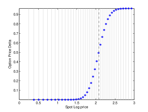
(a) Option Delta

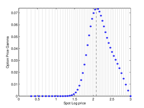
(b) Option Gamma

Figure 1: $C_{S}=0.002$, $r=0.05$, $q_{S}=0.05$, $\gamma_{S}=0.03$, $\sigma=0.1$, $S_{f}=0$, $\lambda_{B}=0.05$, $\lambda_{C}=0.01$, $R_{B}=0.4$, $R_{C}=0.4$, $C_{B}=0.001$, $C_{C}=0.001$, $dt=1/261$, $\Delta\tau=1/261$, $K=8$.

4.2.2 Volatility

Figure (2(a)) presents the sensitivity of the CVA to changes in the volatility parameter. The figure shows that the strike price serves as threshold where the behavior of the CVA changes. When the option is out-of-the money ($S<K$), higher volatility produces higher CVA (more negative). However, when the option is in-the-money ($S>K$), the convexity changes leading to higher CVA as the volatility decreases. Figure (2(b)) expands these results over the entire set of possible volatilities.

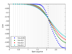
(a) $BK_{TC}$ CVA for different volatilities

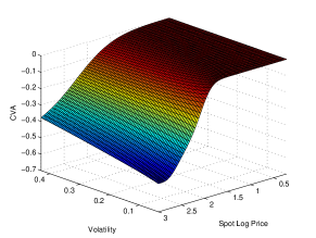
(b) $BK_{TC}$ CVA by Spot Price and Volatility

Figure 2: $C_{S}=0.002$, $q_{S}=0.05$, $\gamma_{S}=0.03$, $r=0.05$, $S_{f}=0$, $\lambda_{C}=0.01$, $R_{C}=0.4$, $\lambda_{B}=0.05$, $R_{B}=0.4$, $C_{B}=0.001$, $C_{C}=0.001$, $dt=1/261$, $\Delta\tau=1/261$, $K=8$.

In Figure (3(a)), the sensitivity of the option price with respect to different volatility parameters is presented. Under the usual Black-Scholes framework, it is expected to get higher option prices as volatility increases. This pattern is confirmed up to a certain spot price. Under our framework, as the option gets deeper in-the-money, Delta (Figure (1(a))), which represents the amount of shares to buy in the replicant strategy, tends to $1$ and the impact of the transaction costs increase by generating a decrease in the option price. This behavior can be confirmed by assessing the first derivative of the option price with respect to the volatility (usually known as Vega). In Figure (4), Vega is split with respect to the moneyness of the option. Figure (4(a)) shows that, when the option is out-of-the-money, Vega is positive as it is under the Black-Scholes model. Further, Figure (4(b)) demonstrate that not only Vega becomes negative as the option gets in-the-money but also that its sign changes in the same spot price as seen in Figure (3(a)). Hence, if we consider the impact of the volatility not only in the parabolic side of the PDE but also in the nonlinear term , it is expected to find these relationship between the volatility parameter and the option price.

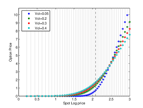
(a) $BK_{TC}$ Option Price for different volatilities

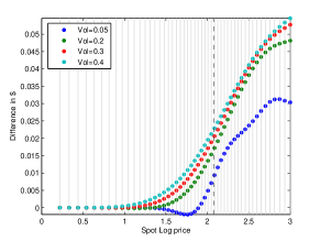
(b) Difference between BK and $BK_{TC}$

Figure 3: $C_{S}=0.002$, $q_{S}=0.05$, $\gamma_{S}=0.03$, $r=0.05$, $S_{f}=0$, $\lambda_{C}=0.01$, $R_{C}=0.4$, $\lambda_{B}=0.05$, $R_{B}=0.4$, $C_{B}=0.001$, $C_{C}=0.001$, $dt=1/261$, $\Delta\tau=1/261$, $K=8$.

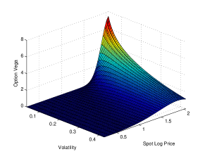
(a) Option Vega out-of-the-money

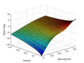
(b) Option Vega in-the-money

Figure 4: $C_{S}=0.002$, $r=0.05$, $q_{S}=0.05$, $\gamma_{S}=0.03$, $\sigma=0.1$, $S_{f}=0$, $\lambda_{B}=0.05$, $\lambda_{C}=0.01$, $R_{B}=0.4$, $R_{C}=0.4$, $C_{B}=0.001$, $C_{C}=0.001$, $dt=1/261$, $\Delta\tau=1/261$, $K=8$.

4.2.3 Interest Rate

Figure (5(a)) presents the sensitivity of the CVA to changes in the interest rate. Figure (5(b)) expand these results to the entire interval of Spot Log prices. Both figures show that the CVA decreases as the interest rate increases and the its size is larger when the option is deep in-the-money.

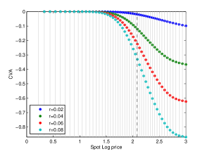
(a) $BK_{TC}$ CVA for different interest rates.

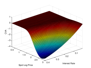
(b) $BK_{TC}$ CVA by Spot price and interest rate.

Figure 5: $C_{S}=0.002$, $q_{S}=0.05$, $\gamma_{S}=0.03$, $\sigma=0.1$, $S_{f}=0$, $\lambda_{C}=0.01$, $R_{C}=0.4$, $\lambda_{B}=0.05$, $R_{B}=0.4$, $C_{B}=0.001$, $C_{C}=0.001$, $dt=1/261$, $\Delta\tau=1/261$, $K=8$.

Figure (6(a)) shows that the option price is a decreasing monotonic function with respect to the interest rate. This result is confirmed by analyzing the first derivative of the option price with respect to the interest rate presented in figure (7), also known as Rho. When the option is out-of-the-money, Rho is approximately equal to zero. But as the option gets in-the-money, it is observed a negative slope. This result is counter-intuitive by considering that, under Black-Scholes model, the derivative is always positive. This discrepancy can be assessed by noting that, in equation (20), the coefficient of $\frac{\partial\hat{V}}{\partial S}S$ is equal to $\,\left(q_{S}-\gamma_{S}\right)$ instead of $\left(r-\gamma_{S}\right)$. Given that under the $BK_{TC}$ model, $q_{S}$ is being modeled as a constant function, the positive sensitivity of the option to the interest rate is not observed. In order to match the expected behavior, an improvement of the modeling approach of the financing cost and its relationship with the interest rate has to be done.

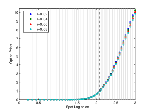
(a) $BK_{TC}$ Option Price for different interest rates

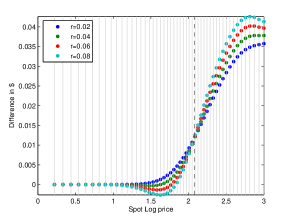
(b) Difference between BK and $BK_{TC}$

Figure 6: $C_{S}=0.002$, $q_{S}=0.05$, $\gamma_{S}=0.03$, $\sigma=0.1$, $S_{f}=0$, $\lambda_{C}=0.01$, $R_{C}=0.4$, $\lambda_{B}=0.05$, $R_{B}=0.4$, $C_{B}=0.001$, $C_{C}=0.001$, $dt=1/261$, $\Delta\tau=1/261$, $K=8$.

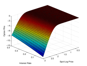
Figure 7: Option Rho

4.2.4 Transaction Costs

Figure (8) presents the variation on the CVA due to changes in the transaction costs that arise of trading $\delta$ amount of shares $S$ and $\alpha_{C}$ amounts of bond $P_{C}$. By recalling equation (20) it can be noted that an increase in $C_{S}$ leads to a decrease in the modified volatility. We actually can assume that the modified volatility behaves similarly to the actual volatility, so that the analysis done in Section 4.2.2 can be applied. By considering the pattern showed in Figure (8) it can be seen that it is in line with the behavior of the CVA when varying the volatility in Figure (8(a)). In both cases, the convexity changes near the strike value due to the same issues presented in the aforementioned section.

On the other side, the presence of $C_{C}$ in Equation (20) actually shows that larger costs generate a lower option price. Also, as transaction costs are multiplied by Delta, the gap widens as the option gets deeper in-the-money. This is the pattern that is observed in Figure (8(b)).

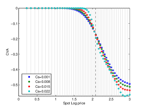
(a) $BK_{TC}$

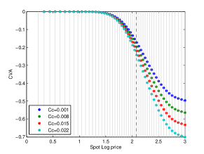
(b) $BK_{TC}$

Figure 8: $r=0.05$, $q_{S}=0.05$, $\gamma_{S}=0.03$, $\sigma=0.1$, $S_{f}=0$, $\lambda_{C}=0.01$, $R_{C}=0.4$, $\lambda_{B}=0.05$, $R_{B}=0.4$, $C_{B}=0.001$, $dt=1/261$, $\Delta\tau=1/261$, $K=8$. $C_{C}=0.001$ for (8(a)) and $C_{S}=0.002$ for (8(b)).

4.2.5 Recovery Rate and Hazard Rate

In Figure (9) the sensitivity of the CVA due to changes in the recovery rate of the counterparty bond is presented. Given that the recovery rate determines the amount of instrument that can be recovered in case of a default, the term $\left(1-R_{C}\right)$ estimates the loss that would arise in case of default. It is expected that higher recovery rates imply lesser losses and then lesser CVA. Figure (9(a)) shows this monotonic relationship which is also in line with the behavior seen in Equation (20).

The hazard rate of the counterparty bond measures the likelihood that the bond will default at a certain point of time. Hence, if the hazard rate increases, the probability of default of the bond also increases. Then, it is expected to see a higher CVA value when deriving the option price. Figure (10(a)) presents the CVA value for different hazard rates where the expected behavior is noticed.

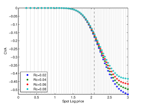
(a) $BK_{TC}$

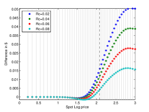
(b) Difference between BK and $BK_{TC}$

Figure 9: $C_{S}=0.002$, $r=0.05$, $q_{S}=0.05$, $\gamma_{S}=0.03$, $\sigma=0.1$, $S_{f}=0$, $\lambda_{C}=0.01$, $\lambda_{B}=0.05$, $R_{B}=0.4$, $C_{B}=0.001$, $C_{C}=0.001$, $dt=1/261$, $\Delta\tau=1/261$, $K=8$

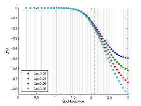
(a) $BK_{TC}$

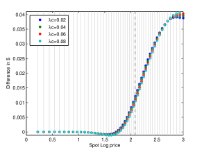
(b) Difference between BK and $BK_{TC}$

Figure 10: $C_{S}=0.002$, $r=0.05$, $q_{S}=0.05$, $\gamma_{S}=0.03$, $\sigma=0.1$, $S_{f}=0$, $\lambda_{B}=0.05$, $R_{B}=0.4$, $R_{C}=0.4$, $C_{B}=0.001$, $C_{C}=0.001$, $dt=1/261$, $\Delta\tau=1/261$, $K=8$.

5 Conclusion

In this work we adapted the PDE formulation of CVA modeling originally proposed in [1] to consider the existence of transaction costs when developing the hedging portfolio. We used the Leland approach to include constant transaction costs applied to trading the spot asset and both counterparty and seller bonds. We constructed a nonlinear PDE model which explains the behavior of an option price considering both counterparty risk and transaction costs. Further, we proved the existence of a solution by applying a fixed-point approach under a constraint in the volatility parameter. Numerical results showed that Delta and Gamma behave similarly as in a plain vanilla option but Vega and Rho presented differences in terms of the usual behavior. It is observed that the presence of transaction costs impact on the way that volatility and risk-free interest rate affects the option price. We also realized that the spot financing cost $q_{S}$ has to be linked with the risk-free interest rate to assure consistent results.

Further work should include the extensions proposed in [1] such as modeling stochastic interest rates, stochastic hazard rates, proposing default time dependency or working with derivatives with more general payments. Nonetheless, the model can be extended by deriving not only a more complex transaction costs function such as the ones used in [17] but also on studying the dynamics of the option price over a basket of assets as in [22].

6 Acknowledgments

This work was partially supported by projects CONICET PIP 11220130100006CO and UBACyT 20020160100002BA.

References

• [1] C. Burgard and M. Kjaer, “Partial differential equation representations of derivatives with bilateral counterparty risk and funding costs,” The Journal of Credit Risk, vol. 7, no. 3, p. 75, 2011.
• [2] F. Black and M. Scholes, “The pricing of options and corporate liabilities,” The Journal of Political Economy, pp. 637–654, 1973.
• [3] J. Gregory, “Being two-faced over counterparty credit risk,” Risk, vol. 22, no. 2, p. 86, 2009.
• [4] A. Green, XVA: Credit, Funding and Capital Valuation Adjustments. John Wiley & Sons, 2015.
• [5] S. Alavian, J. Ding, P. Whitehead, and L. Laudicina, “Counterparty valuation adjustment (cva),” Available at ssrn. com, 2008.
• [6] D. Brigo and K. Chourdakis, “Counterparty risk for credit default swaps: Impact of spread volatility and default correlation,” International Journal of Theoretical and Applied Finance, vol. 12, no. 07, pp. 1007–1026, 2009.
• [7] D. Brigo and A. Capponi, “Bilateral counterparty risk valuation with stochastic dynamical models and application to credit default swaps,” arXiv preprint arXiv:0812.3705, 2008.
• [8] D. Brigo, A. Pallavicini, and V. Papatheodorou, “Arbitrage-free valuation of bilateral counterparty risk for interest-rate products: impact of volatilities and correlations,” International Journal of Theoretical and Applied Finance, vol. 14, no. 06, pp. 773–802, 2011.
• [9] A. Pallavicini, D. Perini, and D. Brigo, “Funding, collateral and hedging: uncovering the mechanics and the subtleties of funding valuation adjustments,” 2012.
• [10] S. Crépey, “A bsde approach to counterparty risk under funding constraints,” Working paper, 2011.
• [11] S. Crépey, “Bilateral counterparty risk under funding constraints—part 1: Pricing,” Mathematical Finance, vol. 25, no. 1, pp. 1–22, 2015.
• [12] S. Crépey, “Bilateral counterparty risk under funding constraints—part 2: Cva,” Mathematical Finance, vol. 25, no. 1, pp. 23–50, 2015.
• [13] H. E. Leland, “Option pricing and replication with transactions costs,” The Journal of Finance, vol. 40, no. 5, pp. 1283–1301, 1985.
• [14] P. P. Boyle and T. Vorst, “Option replication in discrete time with transaction costs,” The Journal of Finance, vol. 47, no. 1, pp. 271–293, 1992.
• [15] T. Hoggard, A. Whalley, and P. Wilmott, “Hedging option portfolios in the presence of transaction costs,” Advances in Futures and Options Research, vol. 7, no. 1, pp. 21–35, 1994.
• [16] P. Amster, C. Averbuj, M. Mariani, and D. Rial, “A black–scholes option pricing model with transaction costs,” Journal of Mathematical Analysis and Applications, vol. 303, no. 2, pp. 688–695, 2005.
• [17] D. Ševčovič and M. Žitňanská, “Analysis of the nonlinear option pricing model under variable transaction costs,” Asia-Pacific Financial Markets, pp. 1–22, 2016.
• [18] I. SenGupta, “Option pricing with transaction costs and stochastic interest rate,” Applied Mathematical Finance, vol. 21, no. 5, pp. 399–416, 2014.
• [19] I. Florescu, M. C. Mariani, and I. Sengupta, “Option pricing with transaction costs and stochastic volatility,” Electronic Journal of Differential Equations, vol. 2014, no. 165, pp. 1–19, 2014.
• [20] V. Zakamouline, “Hedging of option portfolios and options on several assets with transaction costs and nonlinear partial differential equations,” International Journal of Contemporary Mathematical Sciences, vol. 3, no. 4, pp. 159–180, 2008.
• [21] V. Zakamulin, “Option pricing and hedging in the presence of transaction costs and nonlinear partial differential equations,” Available at SSRN 938933, 2008.
• [22] P. Amster and A. P. Mogni, “On a pricing problem for a multi-asset option with general transaction costs,” arXiv preprint arXiv:1704.02036, 2017.
• [23] G. M. Lieberman, Second order parabolic differential equations. World scientific, 1996.
• [24] D. Tavella and C. Randall, Pricing financial instruments: The finite difference method, vol. 13. John Wiley & Sons, 2000.
• [25] J. Bodeau, G. Riboulet, and T. Roncalli, “Non-uniform grids for pde in finance,” 2000.
• [26] S. Foulon et al., “Adi finite difference schemes for option pricing in the heston model with correlation,” International Journal of Numerical Analysis & Modeling, vol. 7, no. 2, pp. 303–320, 2010.
• [27] K. in’t Hout and K. Volders, “Stability of central finite difference schemes on non-uniform grids for the black–scholes equation,” Applied numerical mathematics, vol. 59, no. 10, pp. 2593–2609, 2009.