Identify Susceptible Locations in Medical Records via Adversarial Attacks on Deep Predictive Models
Abstract.
The surging availability of electronic medical records (EHR) leads to increased research interests in medical predictive modeling. Recently many deep learning based predicted models are also developed for EHR data and demonstrated impressive performance. However, a series of recent studies showed that these deep models are not safe: they suffer from certain vulnerabilities. In short, a well-trained deep network can be extremely sensitive to inputs with negligible changes. These inputs are referred to as adversarial examples. In the context of medical informatics, such attacks could alter the result of a high performance deep predictive model by slightly perturbing a patient’s medical records. Such instability not only reflects the weakness of deep architectures, more importantly, it offers a guide on detecting susceptible parts on the inputs. In this paper, we propose an efficient and effective framework that learns a time-preferential minimum attack targeting the LSTM model with EHR inputs, and we leverage this attack strategy to screen medical records of patients and identify susceptible events and measurements. The efficient screening procedure can assist decision makers to pay extra attentions to the locations that can cause severe consequence if not measured correctly. We conduct extensive empirical studies on a real-world urgent care cohort and demonstrate the effectiveness of the proposed screening approach.
1. Introduction
Recent years have witnessed substantial success on applying deep learning techniques in data analysis in various application domains, such as computer vision, natural language processing, and speech recognition. Those modern machine learning techniques have also demonstrated great potentials in clinical informatics (Shickel et al., 2017). For example, deep learning has been used to learn effective representations for patient records (Miotto et al., 2016; Choi et al., 2016b) to support disease phenotyping (Che et al., 2015) and conduct predictive modeling (Che et al., 2016; Pham et al., 2016; Nguyen et al., 2017). A recent study from Google demonstrated the capability of deep learning methods on predictive modeling with electronic health records (EHR) over traditional state-of-art approaches (Alvin Rajkomar, 2018).
Deep learning approaches have a few key advantages over traditional machine learning approaches, including the capability of exploring complicated relationships within the data through the highly non-linear architecture, and building an end-to-end analytics pipeline without the process of handcrafted feature engineering. Most of these perks are backed by complex neural networks and a large volume of training data. However, such complex networks could lead to vulnerable decision boundaries according to statistical learning theory. This effect could be further exacerbated by the sparse, noisy and high-dimensional nature of medical data. For example, in our experiments, we show that a well-trained deep model may classify a dying patient to be healthy when the patient’s record changed a bit, especially for those close to the decision boundary. In addition, certain clinical measurements may be more susceptible to this type of perturbation than others for a given patient. In this work, we propose to take advantage of such vulnerability of deep neural networks to identify susceptible events and measurements in each patient’s medical records such that additional attention from clinicians/nurses is required.
The vulnerability of deep neural networks has been brought up in recent studies, e.g., Szegedy et al. first introduced this concept when investigating the properties of neural networks (Szegedy et al., 2013). They found that even a high-performance deep model can be easily “fooled”, e.g., an image classified correctly by the model can be misclassified with human-imperceptible perturbations. Plenty of later studies demonstrated neural networks to be fragile under these so-called adversarial attacks, where adversarial examples were generated to attack deep models using elegantly designed algorithms. Intuitively, if we can attack a high performance medical predictive model and generate such adversarial medical records from the original medical records of one patient, then these perturbations in the medical records can inform us where the susceptible events/measurements are located.
Currently, most existing attack techniques focused on image related tasks where convolutional neural networks (CNNs) are primarily used. In the medical informatics domain, however, one major focus remains on predictive modeling with sequential medical records (Choi et al., 2016b; Zhou et al., 2014). In order to craft efficient and effective adversarial examples, several challenges persist despite the progress of current attack algorithms. First, unlike images, medical features are heterogeneous, carrying different levels and aspects of information, thus resulting in different tolerance to perturbations. Second, for time sequence data, the effectiveness of perturbations may vary along time, e.g., perturbing a distant time stamp may not work as well as a recent one. Third, since we are interested in utilizing attacks to infer susceptible locations, a sparse attack is preferred over a dense one. However, sparse attacks tend to have larger magnitudes than dense attacks, and no explicit evaluation metrics for sparse attacks has been established yet.
Therefore, to address the aforementioned challenges, we propose an effective and efficient framework for generating adversarial examples for temporal sequence data. Specifically, our sparse adversarial attack approach is based on optimization and can be efficiently solved via an iterative procedure, which automatically learns a time-preferential sparse attack with minimum perturbation on input sequences. From the attack model, we designed a Susceptibility Score for each measurement at both individual-level and population-level, which can be used to screen medical records from different patients and identify vulnerable locations. We also define a new evaluation metric that considers both sparsity and magnitude of a certain attack. We evaluate our attack approach and susceptibility score in the real-world urgent care cohort MIMIC3 (Johnson et al., 2016), and demonstrate the effectiveness of the proposed approach from extensive quantitative and qualitative results. In the context of our paper, we mainly verify our methods on medical data, but the attack framework can be easily extended to any other fields.
2. Related Work
Our work lies in the junction of adversarial attacks and recurrent neural networks on medical informatics. Therefore, we briefly summarize recent advances for both fields in this section.
Recurrent Neural Networks on Medical Informatics. Recurrent neural network (RNN) and its variants, such as gated recurrent unit (GRU) (Cho et al., 2014) and long short-term memory (LSTM) (Hochreiter and Schmidhuber, 1997), are designed for analyzing sequence data and has been widely used in computer vision and natural language processing. Despite the fact that medical records often consist of time series, applications of RNN in medical informatics are much less compared to those in language domain. For example, (Lipton et al., 2015) first utilized LSTM on EHR for multi-label classification of diagnoses and a similar study (Choi et al., 2016a) applied GRU to predict diagnose and medication categories using encounter records. (Baytas et al., 2017) developed a time-aware LSTM to address the differences of time intervals in medical records. Most recently, a comprehensive study (Alvin Rajkomar, 2018) showed superior performance achieved by RNN on predictive modeling with EHR records compared to traditional approaches, calling for more applications of such deep models on medical sequential data. While on the other side, the weakness of deep neural networks was disclosed under more exploration of network properties.
Adversarial Attacks on Deep Networks. Following the discovery of deep network vulnerability, different algorithms have been developed for crafting adversarial examples to better understand the robustness of a deep network. The goal of the attacking algorithm is to crafts an adversarial sample by adding a small perturbation on a clean sample such that the outcome of a deep model changes after the perturbation. Below we briefly introduce adversarial attacks on different types of deep models.
CNN Attacks. There are many existing studies on CNN attacks. Szegedy et al. first introduced adversarial examples for deep learning in (Szegedy et al., 2013), where adversarial examples are obtained by solving an optimization with box-constraints. (Goodfellow et al., 2014) proposed a fast gradient sign method (FGS) that uses the gradient of loss function with respect to input data to generate adversarial examples. In DeepFool (Moosavi-Dezfooli et al., 2016a), an iterative -regularized algorithm is adopted to find the minimum perturbation that changes the result of a classifier. A universal perturbation (Moosavi-Dezfooli et al., 2016b) is also formulated later based on DeepFool. JSMA (Papernot et al., 2016a) is a Jacobian-based saliency map algorithm which creates a direct mapping between inputs and outputs during training, and crafts adversarial examples by modifying a fraction of features (the most influential) iteratively. Instead of leveraging network loss and gradients, Carlini and Wagner (Carlini and Wagner, 2017) proposed new objective functions based on the logit layer to generate adversarial examples (C&W attack). They handle the box-constraint by using a transformation and also consider different distance metrics (, , ). Chen et al. extended C&W attack to distortion metrics and proposed an elastic-net regularized framework (Chen et al., 2017a) for adversarial generation. Zeroth order optimization (ZOO) based attack (Chen et al., 2017b) is a black-box attack algorithm. Different from using network gradients directly, it estimates gradients and Hessian via symmetric difference quotient for crafting adversarial examples. There are other types of adversarial examples like (Nguyen et al., 2015), and other generating approaches including GAN attacks (Zhao et al., 2017), ensemble attacks (Liu et al., 2016), ground truth attacks (Carlini et al., 2017), hot/cold attacks (Rozsa et al., 2016), feature adversary (Sabour et al., 2015) which we do not present further details.
RNN Attacks. Most previous efforts for crafting adversarial examples were made on image classification tasks in the domain of computer vision. Adversarial on deep sequential models are less frequent compared to CNN attacks. For RNN attacks, one focus has been emerged on natural language processing where adversarial examples are generated by adding, removing, or changing words in a sentence (Jia and Liang, 2017; Papernot et al., 2016b; Li et al., 2016). However, those perturbations are usually perceptible to human beings. Another application is on malware detection which is a classification task on sequential inputs. (Grosse et al., 2017) generated adversarial examples by leveraging algorithms of DNN attacks. (Hu and Tan, 2017; Anderson et al., 2016) used GAN based algorithm and (Anderson et al., 2017) used reinforcement learning to generate adversarial examples.
In summary, neither have the aforementioned attacks been used to verify the robustness of RNN models on medical sequence data, nor have they been utilized to provide additional important information located in medical records and thus improves the quality of modern clinical care.
3. Method
Though much of the prior efforts have focused on attack and protect strategies of deep models, in this work, we take a radically different perspective from existing works and leverage the vulnerability of the deep models to inspect the features and data points in the datasets that are sensitive to the complex decision hyperplanes of powerful deep models. When dealing with electronic health records (EHR), such susceptible locations allows us to develop an efficient screening technique for EHR. In this section, we first introduce the problem setting of adversarial attacks, and then propose a novel attack strategy to efficiently identifying susceptible locations. We then use the attacking strategy to derive a susceptibility score which can be deployed in healthcare systems.
The proposed framework of adversarial generation is illustrated in Figure 1. It consists of three parts: (1) building a predictive model which maps time-series EHR data to clinical labels such as diagnoses or mortality, (2) generating adversarial medical records based on the output of the predictive model, and (3) computing the susceptibility score based on the adversarial samples.
3.1. Predictive Modeling from Electronic Medical Records
Medical records for one patient can be represented by a multivariate time series matrix (Baytas et al., 2017; Wang et al., 2012; Zhou et al., 2014). Assume we have a set of medical features in the EHR system and a total of time points available patient , then the patient EHR data can be represented by a matrix . Note that for different patients, the observation length could be different due to the frequency of visits and length of enrollment. At the predictive modeling step, a model is trained to map EHR features of a patient to clinically meaningful labels such as diagnoses, mortality and other clinical assessments. In this paper, we limit our discussions in the scope of classification, i.e., we would like to learn a -class prediction model from our data. We use in-hospital mortality as the running example, where and represent alive and deceased status, respectively. We note that the technique discussed in this paper can be applied to other predictive tasks such as phenotyping and diagnostic prediction.
Recurrent neural networks (RNN) are recently adopted in many predictive modeling studies and achieved state-of-the-art predictive performance, because (1) RNN can naturally handle input data of different lengths and (2) some variants such as long short-term memory (LSTM) networks have demonstrated excellent capability of learning long-term dependencies and are capable of dealing with irregular time interval between time series events (Baytas et al., 2017). Without loss of generality, we use a standard LSTM network as our base predictive model. Given a dataset of patients, , where for each patient we have a set of medical records and a target label . The LSTM network parameters are collected denoted by , and the deep network model is trained by minimizing the following loss function:
where is output of the network. The loss function is minimized by gradient descent via backpropagation algorithm. Let be the parameter obtained by the algorithm from the training dataset , and we denote the final predictive model by .

3.2. Adversarial Medical Records Generation
Our framework is to utilize adversarial attacks to detect susceptible locations in medical records, and an efficient adversarial attack strategy is the key component in this framework. Adversarial examples are usually generated by exploiting internal state information of a high performing pre-trained deep predictive model, which can be the intermediate output or gradients. The existing attack algorithms can be roughly grouped into two prototypes: iterative attacks and optimization-based attacks. The former iteratively add perturbations to original input until some conditions are met. For example, fast gradient sign method (FGS) (Goodfellow et al., 2014) uses gradients of the loss function with respect to input data points to generate adversarial examples.On the other hand, optimization-based attacks cast the generation procedure into an optimization problem in which the perturbation can be analytically computed. Optimization based attacks are shown to have superior performance on adversarial attacks compared to iterative methods (Chen et al., 2017a, b).
In order to generate efficient perturbations for medical records, in this paper we propose an optimization-based attack strategy. Existing attack strategies typically seek a dense perturbation of an input. Jointly perturbing on multiple locations simultaneously can take full advantage of the complexity of the decision surface to achieve minimal perturbation. As long as the magnitude of the perturbed locations is small enough, then it can hardly be perceived by human. However, such dense perturbation strategy is not so meaningful in healthcare, as dense perturbations could easily change the underlying structures of medical records, and introduce comorbidity related to diseases originally not associated with the patient. For example, if a perturbation simultaneously adds the diagnosis features of Hypertension and Heart Failure to a patient who never had these before, it is likely that we are creating new pathology associated to cardiovascular disease. This suggests that focused (sparse) attacks are preferred in our problem.
Formally, given a well performed predictive model, and a patient record , our goal is to find an adversarial medical record of the same size, such that is close to but with a different classification result from the given deep model. Let be a source label currently outputted by the predictive model , and we would like the predictive model to classify into an adversarial class label , while minimizing the difference . As in our mortality prediction example, if a patient is originally predicted to be alive, we would like to find the minimal sparse perturbation to make our model predict the deceased label. We note that it is not necessary for this patient to be a part of the dataset training the model . We propose to obtain the adversarial sample by solving the following sparsity-regularized attack objective:
| (1) |
where Logit() denotes outputs before the Softmax layer in the pre-trained predictive model, ensures a gap between the source label and the adversarial label , and is an element-wise norm. To create adversarial examples with smaller perturbations, is commonly set to 0. The loss function is similar to the one in C&W (Carlini and Wagner, 2017) and EAD attack (Chen et al., 2017a), aiming to assign label the most probable class for . The norm regularization induces sparsity on the perturbation and encourages the desired focused attacks. Additionally, based on the hypothesis that different features have different tolerances and temporal structures might also effect the distribution of susceptible regions, regularization also avoids large perturbations and leads to attacks that have unique structures at both time and feature levels.
Similar to (Chen et al., 2017a), we use the iterative soft thresholding algorithm (ISTA) optimization procedure (Beck and Teboulle, 2009) to solve the objective, where for each record value, the algorithm performs a soft thresholding to shrink a perturbation to 0 if the deviance to original record is less than at each iteration, where soft thresholding performs an element-wise shrinkage of , i.e., . The generation procedure is summarized in Algorithm 1.
Given different strengths of regularization, we end up with a set of adversarial candidates for each medical record matrix. We pick optimal adversarial records based on evaluation metrics below.
3.3. Evaluation of Focused EHR Attacks
Recall that in the detection of susceptible locations in medical records, a focused sparse attack is preferred over a dense one due to the aforementioned reasons. However, using existing attack evaluation metrics such as the magnitude of the perturbation and accuracy of the attacks, a dense one is almost always more efficient than a sparse one because the attacks strategies can fully leverage the complicated decision surface. An analogy is to consider the attacking strategies in the context of the machine learning paradigm. If we perform learning and evaluation on the same training data, then the “best performing” model will be the one that uses no regularization at all, and therefore the testing data is critical for a fair evaluation of the learned model. This is why we need an evaluation strategy that is designed specifically for our attack budget (sparsity).
However, there are currently no metrics in the literature that evaluates both perturbation scale and degree of focus. Therefore, we propose a novel evaluation scheme which measures the quality of a perturbation by considering both the perturbation magnitude and the structure of the attacks. Given an adversarial record , the perturbation is defined as:
Thus, the maximum absolute perturbation for an observation () and the percentage of record values that being perturbed () can be written as:
| (2) |
where is element-wise absolute value. To make perturbations comparable, we normalize our data into [0, 1] range using min-max normalization before any experiments (will be covered in section 4). Since both measures behave like a rate ranging from 0 to 1 and we want both to be small, we define the Perturbation Distance Score metrics as follows:
| (3) |
which geometrically measures a weighted distance between point (, ) and original coordinate. is a weighting parameter that controls which measure is emphasized. In our case, we are more concerned about sparsity and set . The perturbation distance score is used for selecting the best adversarial record for a given observation under different sparsity control. A lower score indicates better quality of perturbation in terms of magnitude and degree of focus.
3.4. Susceptibility Scores for EHR Screening
Besides individual-level perturbation measure, we are also interested in the susceptibility of a certain feature or time stamp at a population-level. These measurements serve to identify the susceptible locations over the entirety of our medical records. We propose three metrics for assessing susceptibility. For simplicity, we assume that the EHR records of all patients have the same length , and we collectively denote the optimal adversarial examples for all patients in a tensor , whose perturbation is denoted by . For the time-feature grid of time stamp and feature , we calculate global maximum perturbation (), global average perturbation () and the probability of being perturbed across all records ():
The susceptibility score for a certain time-feature location is thus defined by:
| (4) |
where denotes element-wise product. The rationale behind this score is the expectation of maximum perturbation for a certain time-measurement grid considering all observations within a population. A larger score indicates high susceptibility of corresponding location with respect to certain diagnose under current predictive model. We also adopt a cumulative susceptibility score for each measurement defined as:
| (5) |
which indicates overall susceptibility at the measurement level.
3.5. Screening Procedure
We summarize here the procedure of the proposed susceptibility screening framework. For each medical record, we utilize the attack algorithm described in Algorithm 1 to perturb the existing deep predictive model until the classification result changes. At each iteration, we evaluate on current adversarial record. Once the result changes, we stop and output the result which can be used for calculating different scores. We picked the optimal adversarial example for each EHR matrix based on perturbation distance score. We then use the adversarial example to compute the susceptibility score for the EHR as well as the cumulative susceptibility score for different measurements.
4. Experiment
4.1. Data Preprocessing
In this work, we use MIMIC-III (Medical Information Mart for Intensive Care III) (Johnson et al., 2016) as our primary data. This dataset contains health-related information for over 45,000 de-identified patients who stayed in the critical care units of the Beth Israel Deaconess Medical Center between 2001 and 2012. MIMIC-III contains information about patient demographics, hourly vital sign measurements, laboratory test results, procedures, medications, ICD-9 codes, caregiver notes and imaging reports.
Our experiment uses records from a collection of patients, each being a multivariate time series consisting of 19 variables from vital sign measurements (6) and lab events (13). Vital signs include heart rate (HR), systolic blood pressure (SBP), diastolic blood pressure (DBP), temperature (TEMP), respiratory rate (RR), and oxygen saturation (SPO2). Lab measurements include: Lactate, partial pressure of carbon dioxide (PaCO2), PH, Albumin (Alb), HCO3, calcium (Ca), creatinine (Cre), glucose (Glc), magnesium (Mg), potassium (K), sodium (Na), blood urea nitrogen (BUN), and Platelet count.
Imputation. MIMIC-III contains numerous missing values and outliers. We first impute missing values using average across time stamps for each record sequence. Then we remove and impute outlier recordings using the interquartile range (IQR) criteria. For each feature, we flatten across all subjects and time stamps and calculate the IQR value. Lower and upper bound values are defined as 1.5 IQR below the first quartile () and 1.5 IQR above the third quartile (). Values out of these bounds are considered as outliers. For each outlier, we impute its value in a carry-forward fashion from the previously available time stamp. If the outlier occurs at the first time stamp, we impute its value using the EHR average across all remaining time stamps.
Padding. One challenge facing EHR data is that time-series recordings are measured asynchronously, often yielding sequential data of different lengths. In previous works, this problem was addressed by taking hourly averages of each feature over the course of an admission (Harutyunyan et al., 2017). This method allows for hourly alignment features for each patient across visits. For our temporal features, the mean length of observation is 60, and median length is 32. We pad all sequences into the same length (48 hours) by pre-padding short sequence using a masking value and pre-truncating long sequences. Therefore all the sequences are aligned to the most recent events and are aligned across each time step.
Normalization. After imputation and padding, we obtain a tensor with three dimensions: observation, time and feature. We normalize using min-max normalization, i.e., for each feature, we collect minimum and maximum values across all observations and time stamps and normalize by:
| (6) |
where the reason is that different measurements have different range and scale, and possibly different tolerance to perturbations. We want to make perturbations among measurements comparable and the calculation of perturbation score more consistent. After normalization, we have 37,559 multivariate time series with 19 variables across 48 time stamps.
| Metric | AUC | F1 | Precision | Recall |
|---|---|---|---|---|
| Avg.SD | 0.90940.0053 | 0.54290.0194 | 0.41000.0272 | 0.80710.0269 |
4.2. Predictive Modeling Performance
Imbalanced data. In order to train a good classifier, we use 5-fold cross-validation. However, among 37,559 observations, there are only 11.1% (4153) deceased labels which make our data highly imbalanced. Therefore, we down-sample observations from the negative class during train-test splitting. We split data into 5 folds in a stratified manner so that the ratio of positive to negative class remains the same as the original dataset on each split. With 5-fold validation, each fold serves as testing fold once, and the other 4 folds become merged and down-sampled to produce balanced training sets. We split the balanced training fold again by 4:1 ratio and treat as training and validation set respectively.
Network Architecture. Considering that an overtly complex architecture may increase the instability of the network, we use a similar architecture as (Lipton et al., 2015) but with simpler settings. Our network contains 3 layers: an LSTM layer, a fully-connected layer followed by soft-max layer. We choose the number of nodes using cross-validation and end up with each layer containing 128, 32 and 2 hidden nodes respectively. We then retrain the entire training folds (training + validation) and assess performance on the testing set, which can be found in Table 1. The resulting LSTM classifier achieves average 0.9094 (0.0053) AUC and 0.5429 (0.0194) f1 score across all folds.
4.3. Susceptibility Detection
We apply the proposed attack framework on correct classified samples and generate susceptibility scores at two levels: patient level and cohort level.
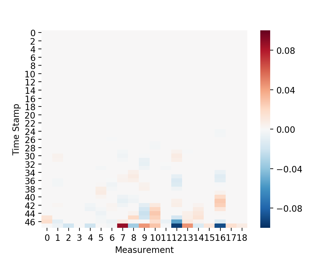
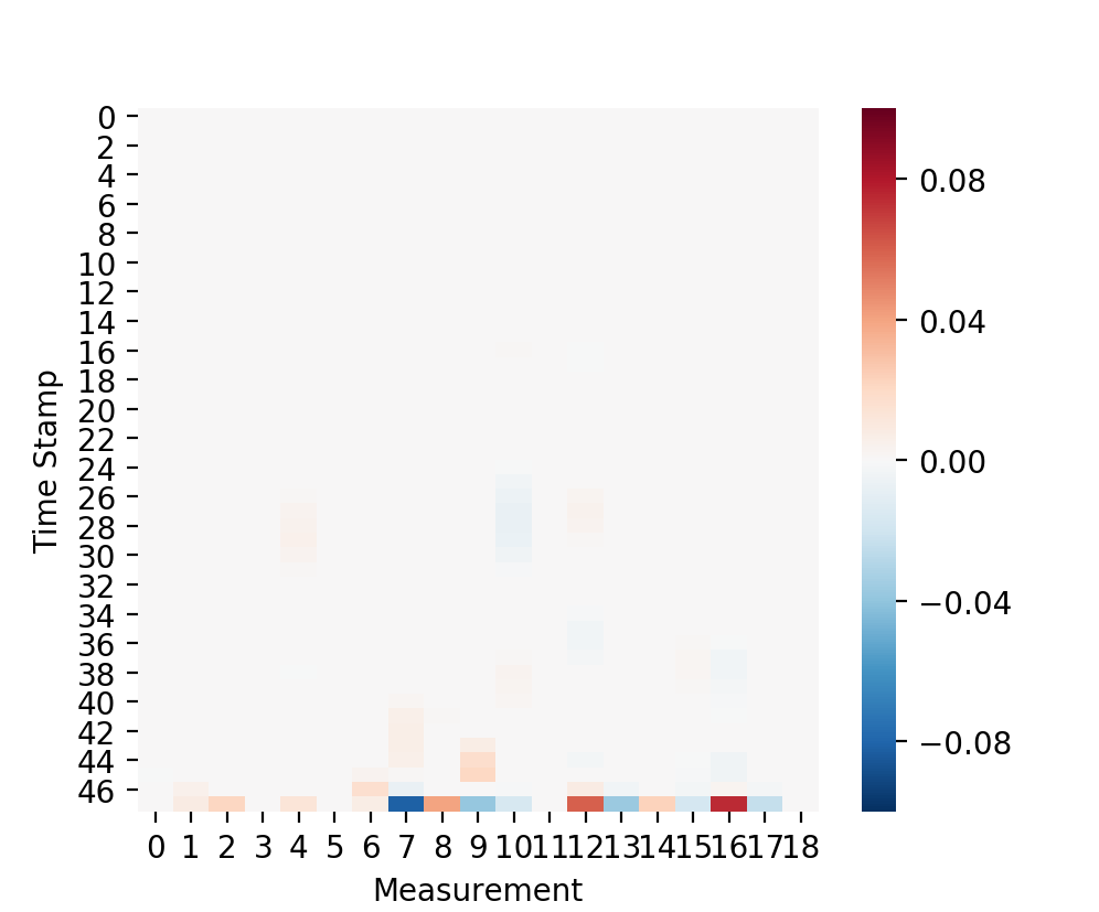
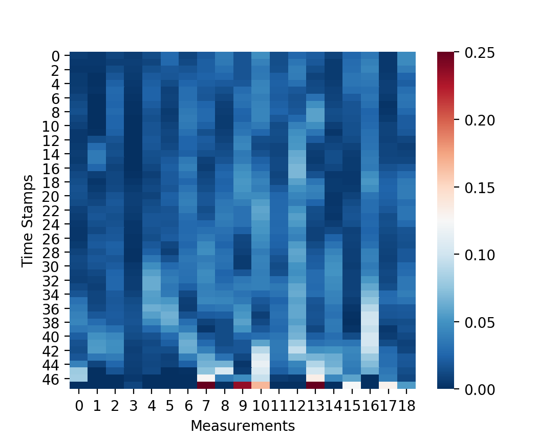
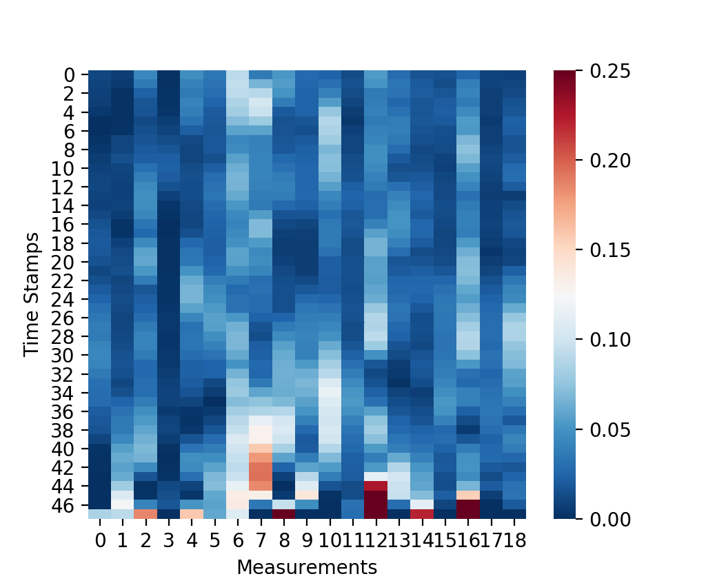
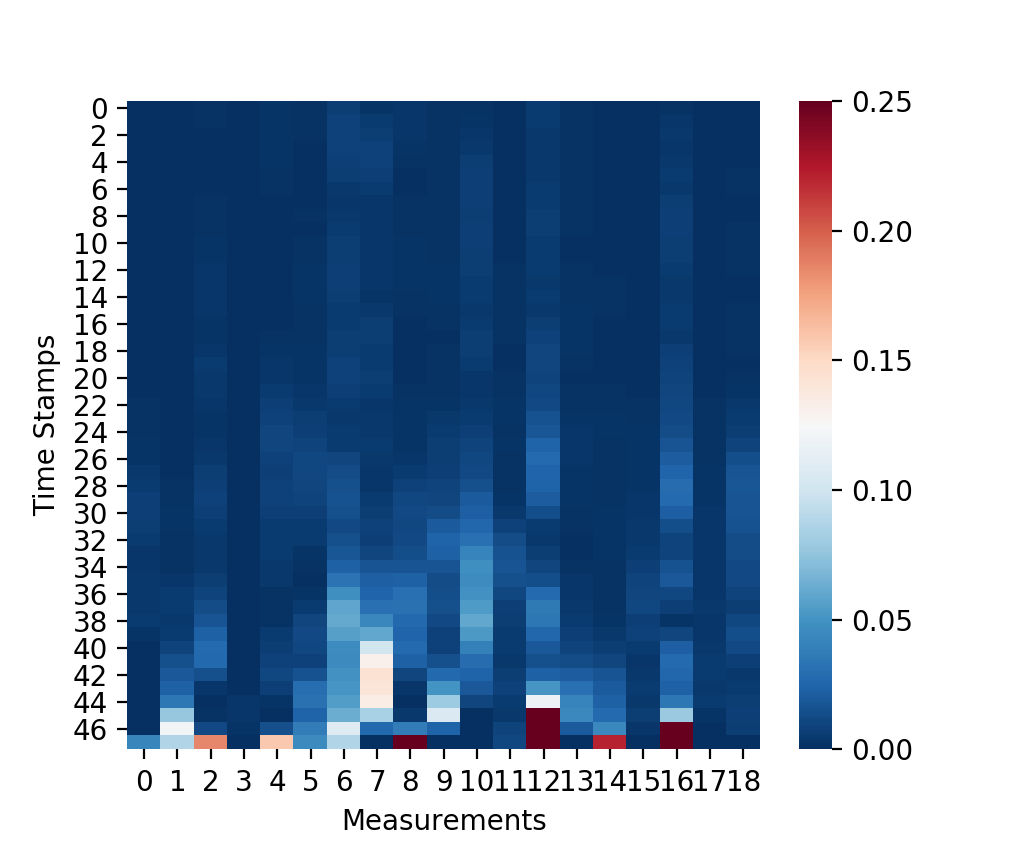
Sensitivity at patient Level. There exists two directions of attacks in binary classification tasks, ie., perturb from negative class to positive and vice versa. Figure 2 shows the adversarial attack results for two patients from each of the attack groups. Figure 2(a) and 2(c) illustrates a distribution of perturbations for a successful adversarial record, ie., . The color represents perturbation magnitude at each measurement and time stamp. Note that the adversarial records which generate the perturbations are chosen from a series of candidate adversarial records via minimizing the perturbation distance score mentioned previously.
We can see that most of the spots are zeros, indicating that no perturbations are made. Among the perturbed locations, we observe a clear pattern along the time axis, which indicates that recent events are more likely to be perturbed compared to distant events. This is consistent with our initial hypothesis that structured perturbation can be more effective. In fact, due to the remember-and-forget mechanism of LSTM networks, the attack algorithm automatically learns to attack this type of model with different degrees of focus for different locations. Our second hypothesis is also verified by the fact that different measurements tend to have varying tolerance to perturbations, as some measurements are not chosen to be attacked while others are more frequently perturbed.
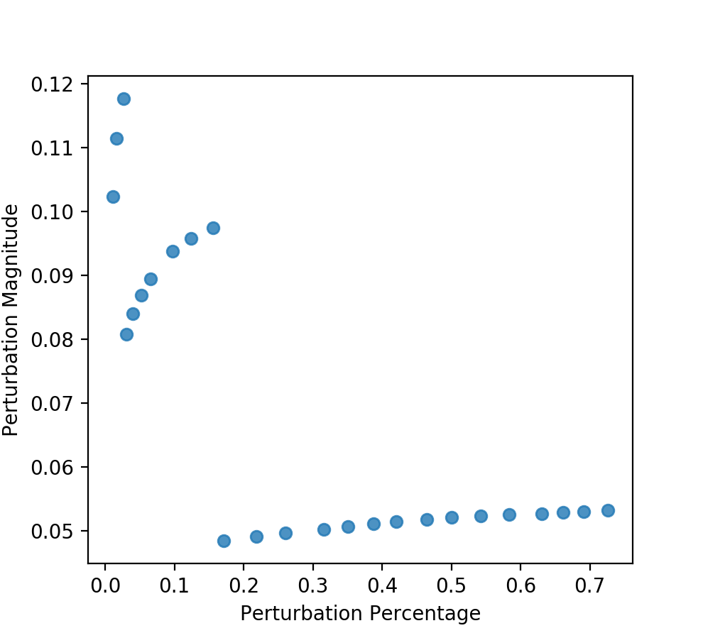
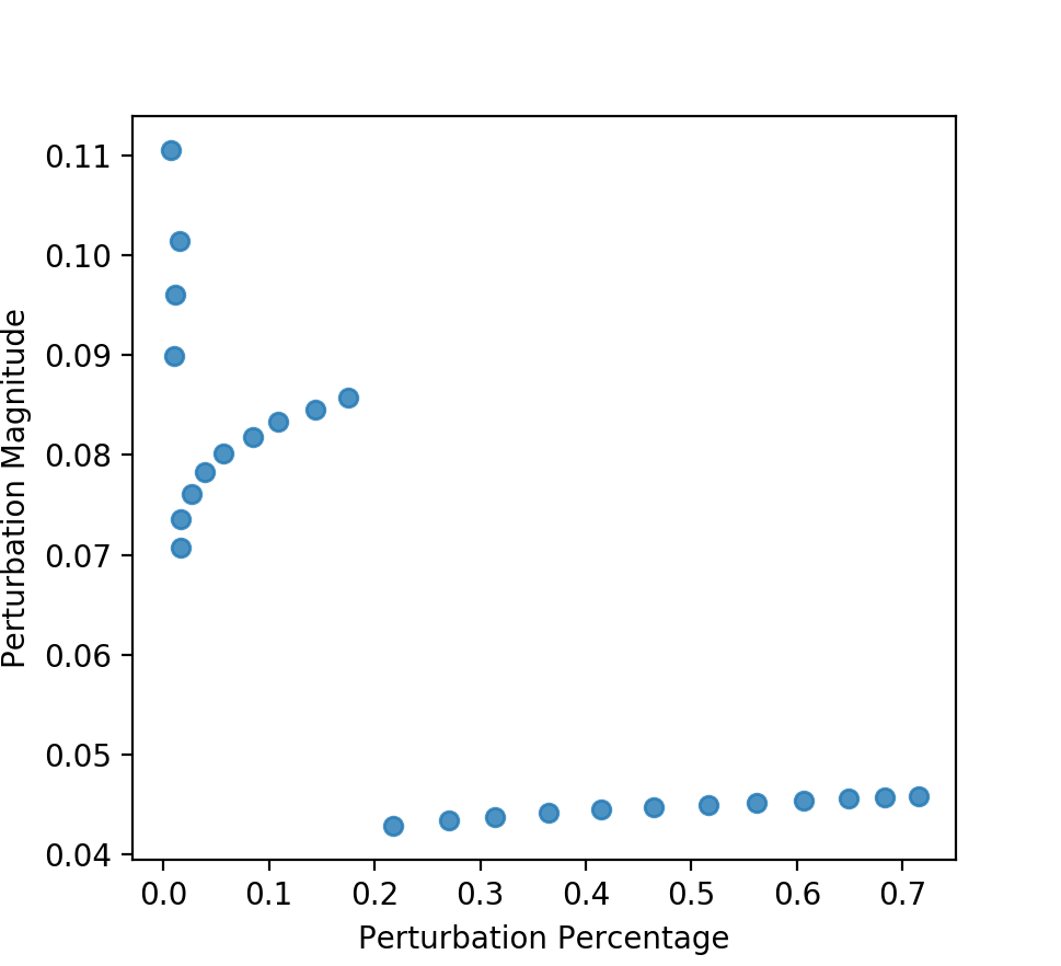
Figure 2(b) and 2(d) presents the maximum perturbation for a patient under different sparsity control. Each regularization parameter generates an adversarial candidate. We can observe the trade-off between perturbation magnitude and sparsity. When only a few spots are attacked, in order to generate success attack, the magnitude of perturbation tends to be large; As more locations change, the perturbation can be flattened to each spot and the magnitude drops quickly. Once over a certain threshold, the maximum perturbation remains similar afterward.
| (0 1) Attack | (1 0) Attack |
 |
 |
| (a) Maximum Perturbation | |
 |
 |
| (b) Average Perturbation | |
 |
 |
| (c) Perturbation Probability | |
Clinical Interpretation By observing the differences in susceptibility to perturbation magnitude and direction across time, clinicians can determine which lab features are robust for consideration in personalized mortality risk assessment. For example, given the perturbation distribution (from an optimal adversarial record) for a patient, we can identify specific regions which warrant increased attention. Given the sample patient in Figure 2(a), we see that arterial carbon dioxide levels (PaCO2), Creatinine (Cre) and Sodium (Na) are more susceptible under the current prediction model. Specifically, we see that increase in PaCO2, decrease in Cre and Na levels render the original classifier susceptible to misclassification. In the reverse case, a comparison between 2(a) and 2(c) reveals that the direction of perturbation on PaCO2, Cre and Na are reversed to achieve misclassification from deceased to alive, which is consistent with our intuition. These results suggest that small errors in Cre, PaCO2 and Na measurements can introduce a significant vulnerability in the mortality assessment of these two sample patients.
Additionally, the direction of perturbation sensitivity can lead to varying interpretation at different time steps. For example, we see from 2(a) and 2(c) that fluctuations in Na levels are susceptible to different directions of perturbation at various time points. At around 8 hours before prediction time (hours 38-44), overestimation in Na levels from laboratory tests renders the classifier susceptible to misclassification toward the alive label, while overestimation at prediction time (48th hour) may cause misclassification toward the deceased label. Perturbation matrix in this case may help guide interpretation of mortality risk with fluctuations in measurement at various time points for certain features.
score distribution.
maximum perturbation.
percentage corresponds to 5(a).
Sensitivity at population Level. While patient-targeted attack reveals vulnerability signals at a personalized level, cohort or population-level analysis is needed to determine the vulnerability of diagnostic features over the entire EHR dataset. Therefore, we also adopt susceptibility score at the cohort level using predefined metrics. We first evaluate performance for a given fold and then extend to all the folds to check for consistency.
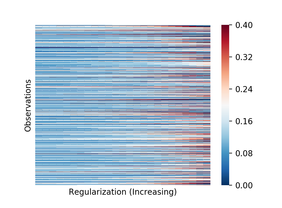
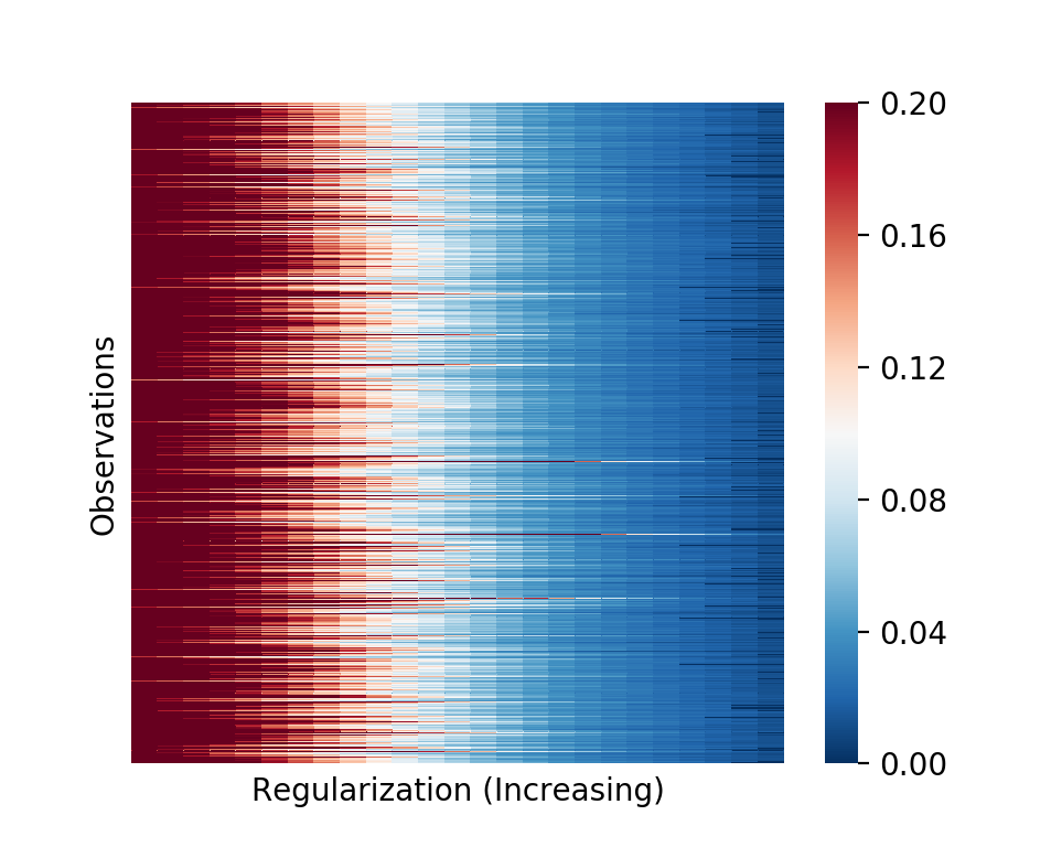
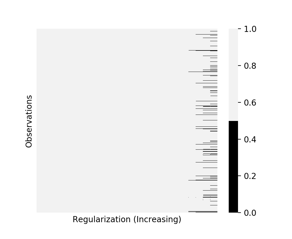
Population-level trade-off. Figure 6 shows the maximum perturbation and percentage of perturbation under different sparsity control at population-level. We can see that as regularization increases, the maximum perturbation increases across all observations. Similarly, there is a more clear pattern for perturbation percentage with respect to regularization. A huge penalty would eventually encourage no spots to be changed and end up with failed adversarial records. Figure 6(c) indicates whether adversarial is successful, 0 for failure 1 for success respectively, across different regularizations. We can see that the attack generate success adversarial records most of the time.
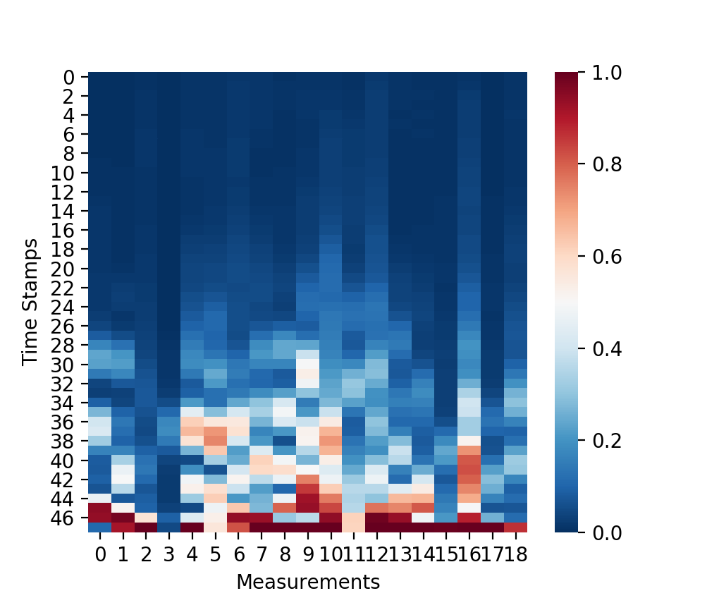
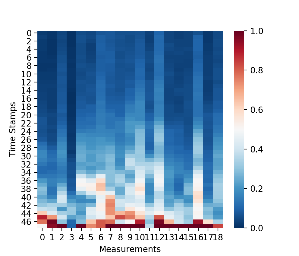
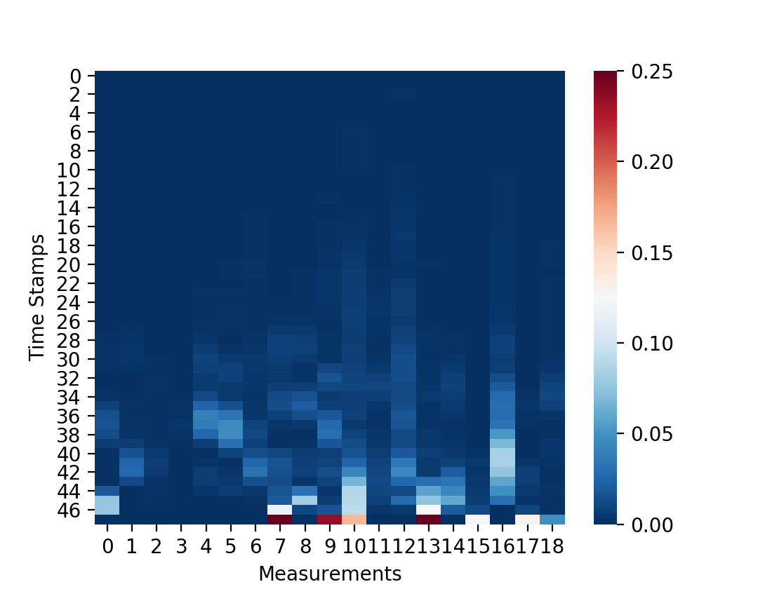
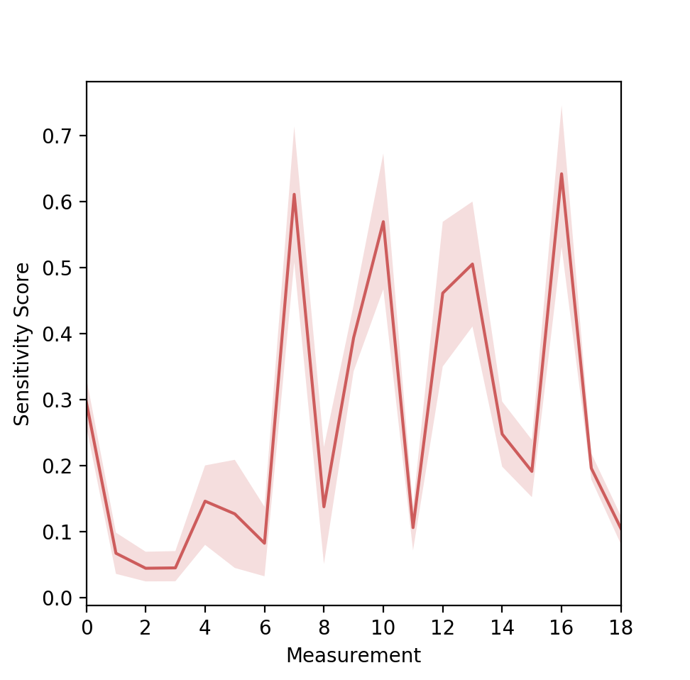
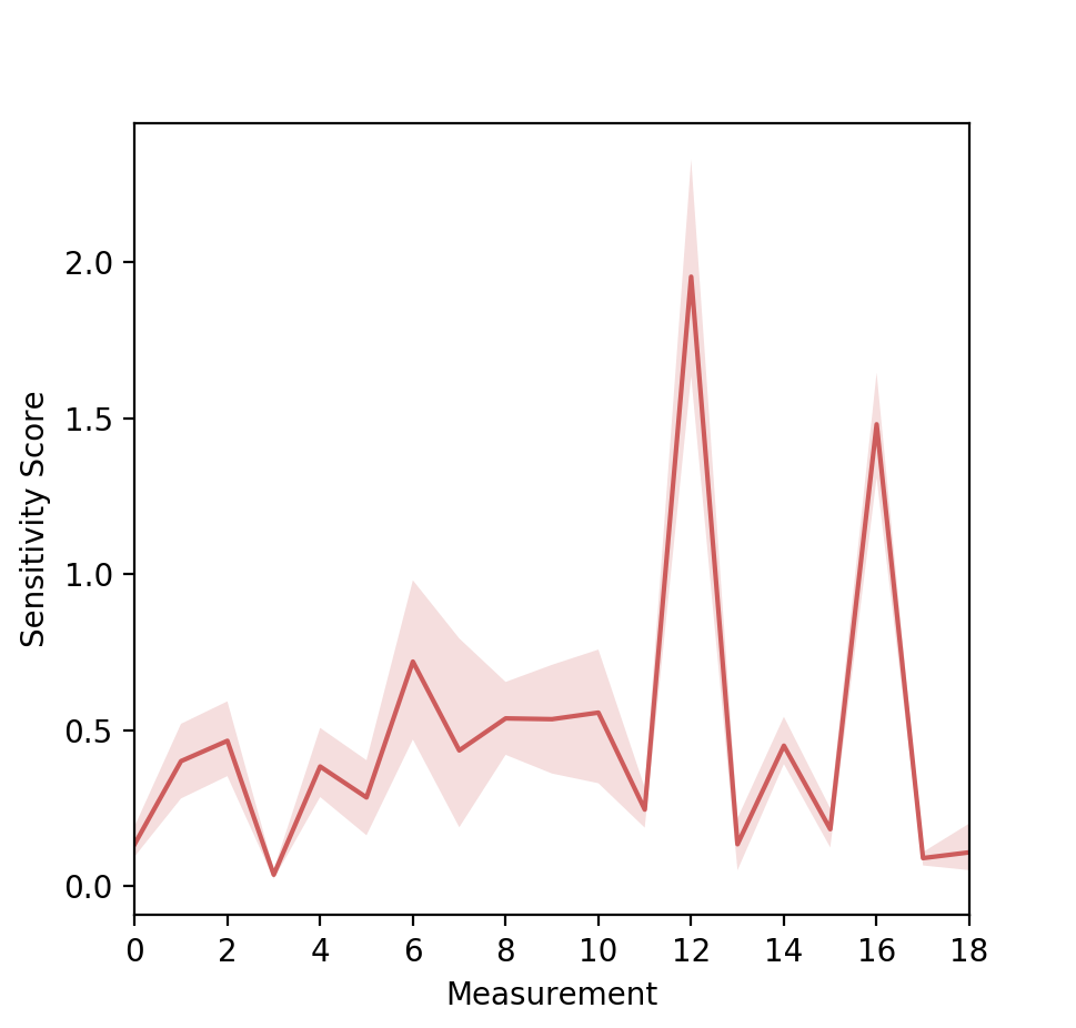
Figure 3 shows the global maximum perturbation (GMP), global average perturbation (GAP) and global perturbation probability (GPP) at each time-measurement grid for 0-1 attack ((left) and 1-0 attack (right) respectively. Figure 4(a) shows the susceptibility score distribution while considering all patients in a fold for 0-1 attack. We can see that measurement PaCO2, Albumin, Glc (7, 9 and 13) at prediction time are the most susceptible locations for mortality prediction model. Similar to the patient-targeted case, not all the measurements have perturbation susceptibility concentrated at the most recent time steps. We observe that measurements RR, SPO2, Na (4, 5 and 16) tends to be more susceptible at earlier time stamps. We repeat evaluation for all 5 folds and found that the results are quite similar. Considering all the time stamps, we obtain a susceptibility score for each measurement by summing the scores across the time axis. Figure 4(b) shows the average sensitivity score and 95% confidence band for each measurement across all 5 folds. Same plots are made for 1-0 attack and can be found at Figure 7. Table 2 shows the ranking of sensitivity for all the measurements.
| Rank | 0-1 Attack | 1-0 Attack | ||
|---|---|---|---|---|
| Measurement | Susceptible Score | Measurement | Susceptible Score | |
| 1 | Na | 0.64 (0.13) | Cre | 1.95 (0.46) |
| 2 | PaCO2 | 0.61 (0.13) | Na | 1.48 (0.21) |
| 3 | HCO3 | 0.57 (0.13) | Lactate | 0.72 (0.33) |
| 4 | Glc | 0.51 (0.12) | HCO3 | 0.56 (0.27) |
| 5 | Cre | 0.46 (0.15) | PH | 0.54 (0.15) |
| 6 | Albumin | 0.39 (0.07) | Albumin | 0.54 (0.23) |
| 7 | HR | 0.30 0.05) | DBP | 0.47 (0.15) |
| 8 | Mg | 0.25 (0.06) | Mg | 0.45 (0.11) |
| 9 | BUN | 0.20 (0.03) | PaCO2 | 0.43 (0.39) |
| 10 | K | 0.19 (0.06) | SBP | 0.40 (0.15) |
| 11 | RR | 0.15 (0.08) | RR | 0.38 (0.14) |
| 12 | PH | 0.14 (0.12) | SPO2 | 0.28 (0.16) |
| 13 | SPO2 | 0.13 (0.11) | Ca | 0.25 (0.08) |
| 14 | Ca | 0.11 (0.04) | K | 0.18 (0.08) |
| 15 | Platelets | 0.10 (0.03) | HR | 0.13 (0.06) |
| 16 | Lactate | 0.08 (0.07) | Glc | 0.13 (0.11) |
| 17 | SBP | 0.07 (0.04) | Platelets | 0.11 (0.10) |
| 18 | TEMP | 0.05 (0.03) | BUN | 0.09 (0.03) |
| 19 | DBP | 0.04 (0.03) | TEMP | 0.04 (0.02) |
Clinical Interpretation Similar to the patient-level patterns, we also observe differences in perturbation sparsity and magnitude across various features at the population-level. Figure 3 (c) shows the probability that a perturbation at certain time steps would lead to misclassification from alive to deceased. This figure can be interpreted as the distribution of susceptibility of each feature across time over the entire EHR dataset. Cold-spots in this grid relate to low probabilities of attack, signaling to the clinician that features associated with those areas are more robust to attack. On the other hand, Figure 3 (b) illustrates the average perturbation over the EHR population for each feature across time. In this grid, we are more concerned about the hot-spots, as cold-spots alone do not rule-out the possibility of LSTM-attack since they only indicate small magnitude of perturbations. However, hot-spots in this grid, indicate preferential spots of LSTM-attack, which rules-in highly susceptible features of the EHR population for misclassification. Figure 3 (a) illustrates the element-wise max perturbation for each feature across all time-steps in the database. As seen from 1, LSTM-attacks are regularized by the magnitude of the perturbation. In the case where the original LSTM classifier is uncertain of the classification decision, the associated data points are closer to the decision boundary, requiring smaller perturbation to achieve misclassification. In the opposite case where data points are further away from the classifier decision boundary, more perturbation is required to cause misclassification. Thus, the max-perturbation grid shown in 3 (a) represents the average LSTM prediction certainty over the EHR record samples; a max-perturbation grid that is dominated by cold-spots reflects a classifier that is mostly uncertain of its predictions, yielding to small perturbations required for misclassification. A max-perturbation grid that is hot-spot dominant indicates a classifier that is highly certain of its predictions, as max-thresholds of perturbation required is higher for most of its samples.
Additionally, these results may be used to provide clinical decision support in determining the optimal rate of sampling for individual clinical features. For example, while vital signs (features 0-5) are obtained at all times for each patient admitted to the urgent care, laboratory tests such as comprehensive metabolic panels (CMP) are much more costly to obtain, especially for patients who require a long length of stays (Hsia et al., 2014). Using our attack framework, a clinician can opt to perform an initial prediction at the beginning of an admission to gauge mortality risk of a patient, and then determine the sampling rate for certain laboratory tests depending on the susceptibility score of the clinical feature to perturbations across time. For example, Table 2 can give clinicians an initial interpretation of the validity of the mortality risk obtained from a prediction model at admission time, while Figure 4 may inform when and how frequently subsequent laboratory tests should be done to update mortality risk evaluation. By sampling at an optimal rate which adjusts for perturbation of measurements across time, clinicians can potentially save cost associated with frequent use of expensive diagnostic tests without sacrificing the accuracy of clinical assessment.
4.4. Adversarial assessment.
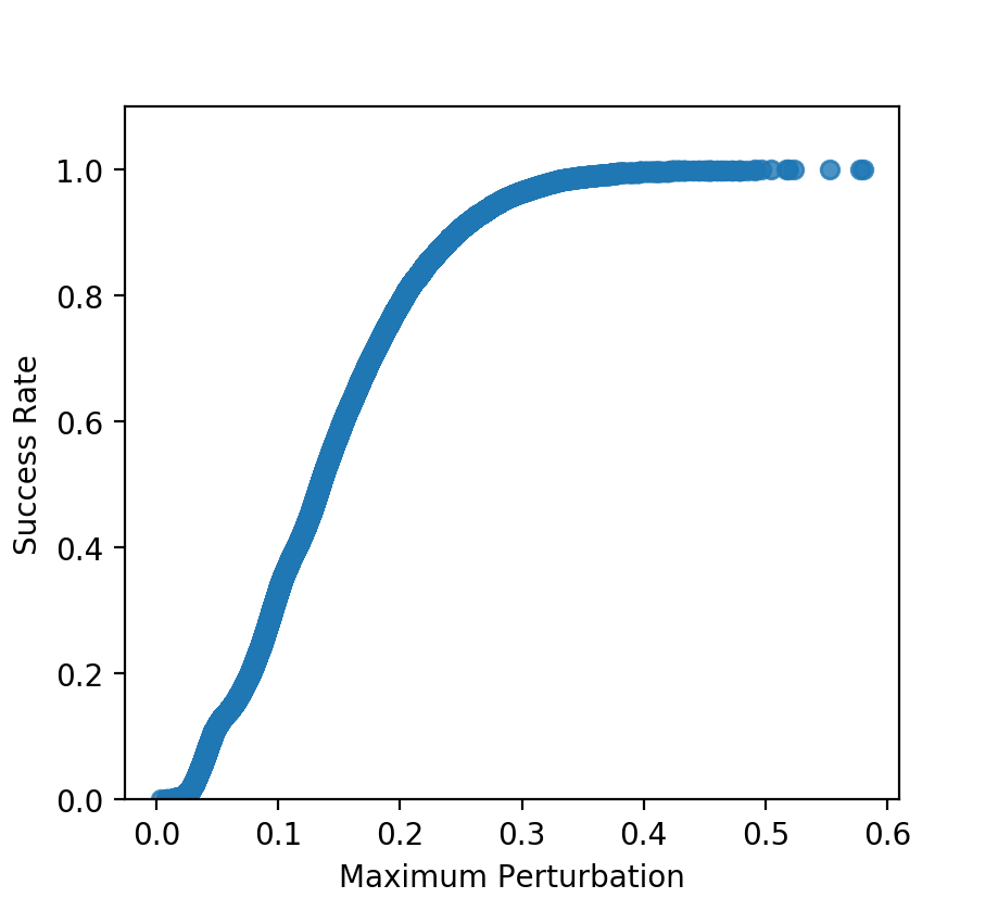
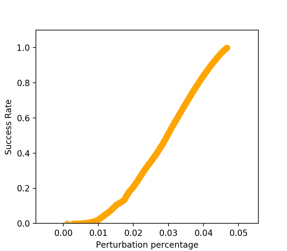
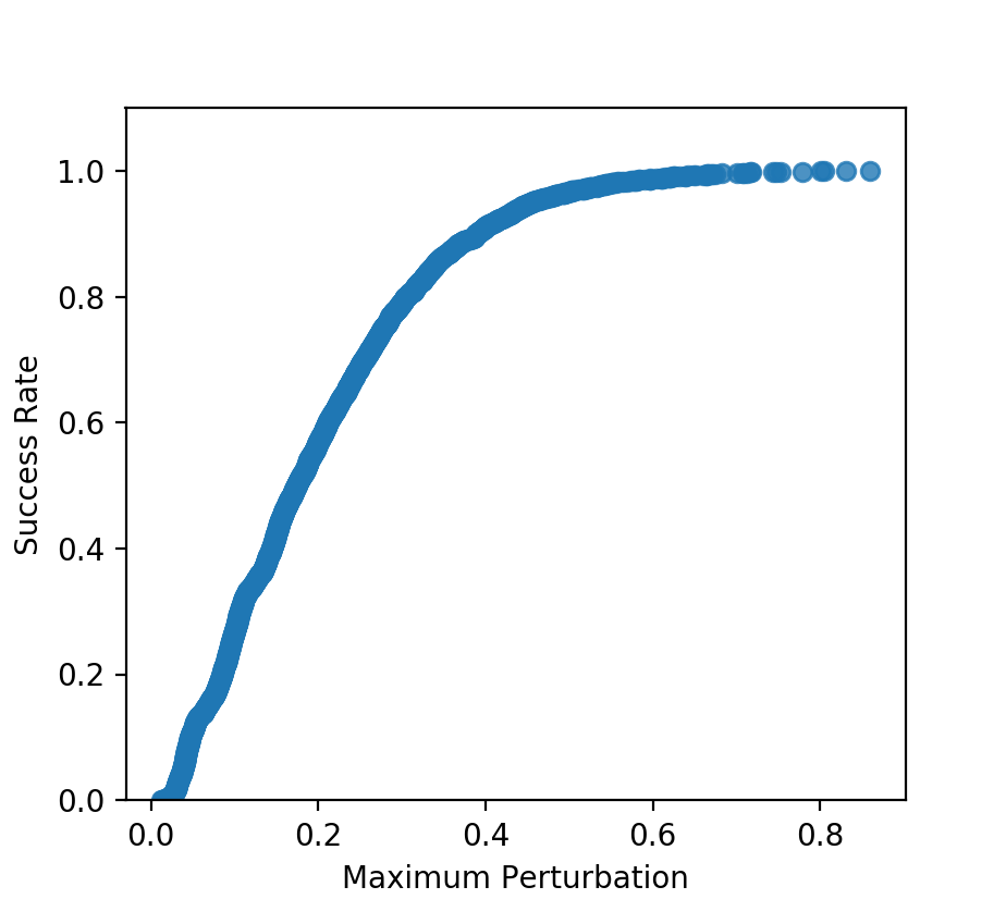
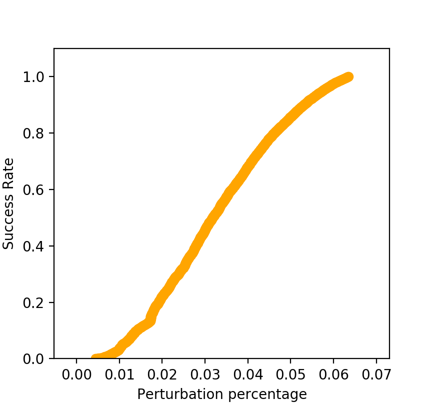
While our ultimate goal is to utilize attack results to detect susceptibility locations of clinical records, we do not enforce strict constraints on the attacks. We assess our adversarial attack by success rate achieved at different maximum perturbation across all patients and the corresponding perturbation percentage at each stage. Results are shown in Figure 5. We can see that more than half of the patients can be perturbed with maximum perturbation less than 0.15 by only changing 3% of the record locations for 0-1 attack. The 1-0 direction is relatively harder to attack compared to the other.
maximum perturbation.
percentage corresponds to 8(a).
5. Conclusion
In this paper, we proposed an efficient and effective framework that identifies susceptible locations in medical records utilizing adversarial attacks on deep predictive models. Our results demonstrated the vulnerability of deep models, where more than half of the patients can be successfully attacked by changing only 3% of the record locations with maximum perturbation less than 0.15 and average perturbation less than 0.02. The proposed screening approach can detect susceptible events and locations at both patient and population level, providing valuable information and assistance for clinical professionals. In addition, the framework can be easily extend to other predictive modeling on time series data.
Acknowledgements.
This research is supported in part by National Science Foundation under Grant IIS-1565596 (JZ), IIS-1615597 (JZ), IIS-1650723 (FW) and IIS-1716432 (FW). and the Office of Naval Research under grant number N00014-14-1-0631 (JZ) and N00014-17-1-2265 (JZ).References
- (1)
- Alvin Rajkomar (2018) Eyal Oren et. al Alvin Rajkomar. 2018. Scalable and accurate deep learning for electronic health records. arXiv preprint arXiv:1801.07860 (2018).
- Anderson et al. (2017) Hyrum S Anderson, Anant Kharkar, Bobby Filar, and Phil Roth. 2017. Evading machine learning malware detection. Black Hat (2017).
- Anderson et al. (2016) Hyrum S Anderson, Jonathan Woodbridge, and Bobby Filar. 2016. DeepDGA: Adversarially-Tuned Domain Generation and Detection. In Proceedings of the 2016 ACM Workshop on Artificial Intelligence and Security. ACM, 13–21.
- Baytas et al. (2017) Inci M Baytas, Cao Xiao, Xi Zhang, Fei Wang, Anil K Jain, and Jiayu Zhou. 2017. Patient subtyping via time-aware LSTM networks. In Proceedings of the 23rd ACM SIGKDD International Conference on Knowledge Discovery and Data Mining. ACM, 65–74.
- Beck and Teboulle (2009) Amir Beck and Marc Teboulle. 2009. A fast iterative shrinkage-thresholding algorithm for linear inverse problems. SIAM journal on imaging sciences 2, 1 (2009), 183–202.
- Carlini et al. (2017) Nicholas Carlini, Guy Katz, Clark Barrett, and David L Dill. 2017. Ground-Truth Adversarial Examples. arXiv preprint arXiv:1709.10207 (2017).
- Carlini and Wagner (2017) Nicholas Carlini and David Wagner. 2017. Towards evaluating the robustness of neural networks. In Security and Privacy (SP), 2017 IEEE Symposium on. IEEE, 39–57.
- Che et al. (2015) Zhengping Che, David Kale, Wenzhe Li, Mohammad Taha Bahadori, and Yan Liu. 2015. Deep computational phenotyping. In Proceedings of the 21th ACM SIGKDD International Conference on Knowledge Discovery and Data Mining. ACM, 507–516.
- Che et al. (2016) Zhengping Che, Sanjay Purushotham, Robinder Khemani, and Yan Liu. 2016. Interpretable deep models for icu outcome prediction. In AMIA Annual Symposium Proceedings, Vol. 2016. American Medical Informatics Association, 371.
- Chen et al. (2017a) Pin-Yu Chen, Yash Sharma, Huan Zhang, Jinfeng Yi, and Cho-Jui Hsieh. 2017a. EAD: Elastic-Net Attacks to Deep Neural Networks via Adversarial Examples. arXiv preprint arXiv:1709.04114 (2017).
- Chen et al. (2017b) Pin-Yu Chen, Huan Zhang, Yash Sharma, Jinfeng Yi, and Cho-Jui Hsieh. 2017b. Zoo: Zeroth order optimization based black-box attacks to deep neural networks without training substitute models. In Proceedings of the 10th ACM Workshop on Artificial Intelligence and Security. ACM, 15–26.
- Cho et al. (2014) Kyunghyun Cho, Bart Van Merriënboer, Caglar Gulcehre, Dzmitry Bahdanau, Fethi Bougares, Holger Schwenk, and Yoshua Bengio. 2014. Learning phrase representations using RNN encoder-decoder for statistical machine translation. arXiv preprint arXiv:1406.1078 (2014).
- Choi et al. (2016a) Edward Choi, Mohammad Taha Bahadori, Andy Schuetz, Walter F Stewart, and Jimeng Sun. 2016a. Doctor ai: Predicting clinical events via recurrent neural networks. In Machine Learning for Healthcare Conference. 301–318.
- Choi et al. (2016b) Edward Choi, Mohammad Taha Bahadori, Elizabeth Searles, Catherine Coffey, Michael Thompson, James Bost, Javier Tejedor-Sojo, and Jimeng Sun. 2016b. Multi-layer representation learning for medical concepts. In Proceedings of the 22nd ACM SIGKDD International Conference on Knowledge Discovery and Data Mining. ACM, 1495–1504.
- Goodfellow et al. (2014) Ian J Goodfellow, Jonathon Shlens, and Christian Szegedy. 2014. Explaining and harnessing adversarial examples. arXiv preprint arXiv:1412.6572 (2014).
- Grosse et al. (2017) Kathrin Grosse, Nicolas Papernot, Praveen Manoharan, Michael Backes, and Patrick McDaniel. 2017. Adversarial examples for malware detection. In European Symposium on Research in Computer Security. Springer, 62–79.
- Harutyunyan et al. (2017) Hrayr Harutyunyan, Hrant Khachatrian, David C Kale, and Aram Galstyan. 2017. Multitask Learning and Benchmarking with Clinical Time Series Data. arXiv preprint arXiv:1703.07771 (2017).
- Hochreiter and Schmidhuber (1997) Sepp Hochreiter and Jürgen Schmidhuber. 1997. Long short-term memory. Neural computation 9, 8 (1997), 1735–1780.
- Hsia et al. (2014) Renee Y Hsia, Yaa Akosa Antwi, and Julia P Nath. 2014. Variation in charges for 10 common blood tests in California hospitals: a cross-sectional analysis. BMJ open 4, 8 (2014), e005482.
- Hu and Tan (2017) Weiwei Hu and Ying Tan. 2017. Generating Adversarial Malware Examples for Black-Box Attacks Based on GAN. arXiv preprint arXiv:1702.05983 (2017).
- Jia and Liang (2017) Robin Jia and Percy Liang. 2017. Adversarial examples for evaluating reading comprehension systems. arXiv preprint arXiv:1707.07328 (2017).
- Johnson et al. (2016) Alistair EW Johnson, Tom J Pollard, Lu Shen, H Lehman Li-wei, Mengling Feng, Mohammad Ghassemi, Benjamin Moody, Peter Szolovits, Leo Anthony Celi, and Roger G Mark. 2016. MIMIC-III, a freely accessible critical care database. Scientific data 3 (2016), 160035.
- Li et al. (2016) Jiwei Li, Will Monroe, and Dan Jurafsky. 2016. Understanding Neural Networks through Representation Erasure. arXiv preprint arXiv:1612.08220 (2016).
- Lipton et al. (2015) Zachary C Lipton, David C Kale, Charles Elkan, and Randall Wetzel. 2015. Learning to diagnose with LSTM recurrent neural networks. arXiv preprint arXiv:1511.03677 (2015).
- Liu et al. (2016) Yanpei Liu, Xinyun Chen, Chang Liu, and Dawn Song. 2016. Delving into transferable adversarial examples and black-box attacks. arXiv preprint arXiv:1611.02770 (2016).
- Miotto et al. (2016) Riccardo Miotto, Li Li, Brian A Kidd, and Joel T Dudley. 2016. Deep patient: an unsupervised representation to predict the future of patients from the electronic health records. Scientific reports 6 (2016), 26094.
- Moosavi-Dezfooli et al. (2016b) Seyed-Mohsen Moosavi-Dezfooli, Alhussein Fawzi, Omar Fawzi, and Pascal Frossard. 2016b. Universal adversarial perturbations. arXiv preprint arXiv:1610.08401 (2016).
- Moosavi-Dezfooli et al. (2016a) Seyed-Mohsen Moosavi-Dezfooli, Alhussein Fawzi, and Pascal Frossard. 2016a. Deepfool: a simple and accurate method to fool deep neural networks. In Proceedings of the IEEE Conference on Computer Vision and Pattern Recognition. 2574–2582.
- Nguyen et al. (2015) Anh Nguyen, Jason Yosinski, and Jeff Clune. 2015. Deep neural networks are easily fooled: High confidence predictions for unrecognizable images. In Proceedings of the IEEE Conference on Computer Vision and Pattern Recognition. 427–436.
- Nguyen et al. (2017) Phuoc Nguyen, Truyen Tran, Nilmini Wickramasinghe, and Svetha Venkatesh. 2017. Deepr: A Convolutional Net for Medical Records. IEEE journal of biomedical and health informatics 21, 1 (2017), 22–30.
- Papernot et al. (2016a) Nicolas Papernot, Patrick McDaniel, Somesh Jha, Matt Fredrikson, Z Berkay Celik, and Ananthram Swami. 2016a. The limitations of deep learning in adversarial settings. In Security and Privacy (EuroS&P), 2016 IEEE European Symposium on. IEEE, 372–387.
- Papernot et al. (2016b) Nicolas Papernot, Patrick McDaniel, Ananthram Swami, and Richard Harang. 2016b. Crafting adversarial input sequences for recurrent neural networks. In Military Communications Conference, MILCOM 2016-2016 IEEE. IEEE, 49–54.
- Pham et al. (2016) Trang Pham, Truyen Tran, Dinh Phung, and Svetha Venkatesh. 2016. Deepcare: A deep dynamic memory model for predictive medicine. In Pacific-Asia Conference on Knowledge Discovery and Data Mining. Springer, 30–41.
- Rozsa et al. (2016) Andras Rozsa, Ethan M Rudd, and Terrance E Boult. 2016. Adversarial diversity and hard positive generation. In Proceedings of the IEEE Conference on Computer Vision and Pattern Recognition Workshops. 25–32.
- Sabour et al. (2015) Sara Sabour, Yanshuai Cao, Fartash Faghri, and David J Fleet. 2015. Adversarial manipulation of deep representations. arXiv preprint arXiv:1511.05122 (2015).
- Shickel et al. (2017) Benjamin Shickel, Patrick James Tighe, Azra Bihorac, and Parisa Rashidi. 2017. Deep EHR: A Survey of Recent Advances in Deep Learning Techniques for Electronic Health Record (EHR) Analysis. IEEE Journal of Biomedical and Health Informatics (2017).
- Szegedy et al. (2013) Christian Szegedy, Wojciech Zaremba, Ilya Sutskever, Joan Bruna, Dumitru Erhan, Ian Goodfellow, and Rob Fergus. 2013. Intriguing properties of neural networks. arXiv preprint arXiv:1312.6199 (2013).
- Wang et al. (2012) Fei Wang, Noah Lee, Jianying Hu, Jimeng Sun, and Shahram Ebadollahi. 2012. Towards heterogeneous temporal clinical event pattern discovery: a convolutional approach. In Proceedings of the 18th ACM SIGKDD international conference on Knowledge discovery and data mining. ACM, 453–461.
- Zhao et al. (2017) Zhengli Zhao, Dheeru Dua, and Sameer Singh. 2017. Generating Natural Adversarial Examples. arXiv preprint arXiv:1710.11342 (2017).
- Zhou et al. (2014) Jiayu Zhou, Fei Wang, Jianying Hu, and Jieping Ye. 2014. From micro to macro: data driven phenotyping by densification of longitudinal electronic medical records. In Proceedings of the 20th ACM SIGKDD international conference on Knowledge discovery and data mining. ACM, 135–144.