Stochastic Variance-Reduced Hamilton Monte Carlo Methods

Abstract

We propose a fast stochastic Hamilton Monte Carlo (HMC) method, for sampling from a smooth and strongly log-concave distribution. At the core of our proposed method is a variance reduction technique inspired by the recent advance in stochastic optimization. We show that, to achieve $\epsilon$ accuracy in 2-Wasserstein distance, our algorithm achieves $\widetilde{O}\big{(}n+\kappa^{2}d^{1/2}/\epsilon+\kappa^{4/3}d^{1/3}n^{2/3}/\epsilon^{2/3}\big{)}$ gradient complexity (i.e., number of component gradient evaluations), which outperforms the state-of-the-art HMC and stochastic gradient HMC methods in a wide regime. We also extend our algorithm for sampling from smooth and general log-concave distributions, and prove the corresponding gradient complexity as well. Experiments on both synthetic and real data demonstrate the superior performance of our algorithm.

1 Introduction

Past decades have witnessed increasing attention of Markov Chain Monte Carlo (MCMC) methods in modern machine learning problems (Andrieu et al., 2003). An important family of Markov Chain Monte Carlo algorithms, called Langevin Monte Carlo method (Neal et al., 2011), is proposed based on Langevin dynamics (Parisi, 1981). Langevin dynamics was used for modeling of the dynamics of molecular systems, and can be described by the following Itô’s stochastic differential equation (SDE) (Øksendal, 2003),

$$d\bm{X}_{t}=-\nabla f(\bm{X}_{t})dt+\sqrt{2\beta}\text{d}\bm{B}_{t},$$ (1.1)

where $\bm{X}_{t}$ is a $d$-dimensional stochastic process, $t\geq 0$ denotes the time index, $\beta>0$ is the temperature parameter, and $\bm{B}_{t}$ is the standard $d$-dimensional Brownian motion. Under certain assumptions on the drift coefficient $\nabla f$, Chiang et al. (1987) showed that the distribution of $\bm{X}_{t}$ in (1.1) converges to its stationary distribution, a.k.a., the Gibbs measure $\pi_{\beta}\propto\exp(-\beta f(\mathbf{x}))$. Note that $\pi_{\beta}$ is smooth and log-concave (resp. strongly log-concave) if $f$ is smooth and convex (resp. strongly convex). A typical way to sample from density $\pi_{\beta}$ is applying Euler-Maruyama discretization scheme (Kloeden & Platen, 1992) to (1.1), which yields

$$\bm{X}_{k+1}=\bm{X}_{k}-\nabla f(\bm{X}_{k})\eta+\sqrt{2\eta\beta}\cdot\bm{\epsilon}_{k},$$ (1.2)

where $\bm{\epsilon}_{k}\sim N(\mathbf{0},\mathbf{I}_{d\times d})$ is a standard Gaussian random vector, $\mathbf{I}_{d\times d}$ is a $d\times d$ identity matrix, and $\eta>0$ is the step size. (1.2) is often referred to as the Langevin Monte Carlo (LMC) method. In total variation (TV) distance, LMC has been proved to be able to produce approximate sampling of density $\pi_{\beta}\propto e^{-f/\beta}$ under arbitrary precision requirement in Dalalyan (2014); Durmus & Moulines (2016b), with properly chosen step size. The non-asymptotic convergence of LMC has also been studied in Dalalyan (2017); Dalalyan & Karagulyan (2017); Durmus et al. (2017), which shows that the LMC algorithm can achieve $\epsilon$-precision in $2$-Wasserstein distance after $\widetilde{O}(\kappa^{2}d/\epsilon^{2})$ iterations if $f$ is $L$-smooth and $\mu$-strongly convex, where $\kappa=L/\mu$ is the condition number.

In order to accelerate the convergence of Langevin dynamics (1.1) and improve its mixing time to the unique stationary distribution, Hamiltonian dynamics (Duane et al., 1987; Neal et al., 2011) was proposed, which is also known as underdampled Langevin dynamics and is defined by the following system of SDEs

$$\begin{split}\text{d}\bm{V}_{t}&=-\gamma\bm{V}_{t}\text{d}t-u\nabla f(\bm{X}_{t})\text{d}t+\sqrt{2\gamma u}\text{d}\bm{B}_{t},\\ \text{d}\bm{X}_{t}&=\bm{V}_{t}\text{d}t,\end{split}$$ (1.3)

where $\gamma>0$ is the friction parameter, $u$ denotes the inverse mass, $\bm{X}_{t},\bm{V}_{t}\in\mathbb{R}^{d}$ are the position and velocity of the continuous-time dynamics respectively, and $\bm{B}_{t}$ is the Brownian motion. Let $\bm{W}_{t}=(\bm{X}_{t}^{\top},\bm{V}_{t}^{\top})^{\top}$, under mild assumptions on the drift coefficient $\nabla f(\mathbf{x})$, the distribution of $\bm{W}_{t}$ converges to an unique invariant distribution $\pi_{\mathbf{w}}\propto e^{-f(\mathbf{x})-\|\mathbf{v}\|_{2}^{2}/(2u)}$ (Neal et al., 2011), whose marginal distribution on $\bm{X}_{t}$, denoted by $\pi$, is proportional to $e^{-f(\mathbf{x})}$. Similar to the numerical approximation of the Langevin dynamics in (1.2), one can also apply the same Euler-Maruyama discretization scheme to Hamiltonian dynamics in (1.3), which gives rise to Hamiltonian Monte Carlo (HMC) method

$$\begin{split}\mathbf{v}_{k+1}&=\mathbf{v}_{k}-\gamma\eta\mathbf{v}_{k}-\eta u\nabla f(\mathbf{x}_{k})+\sqrt{2\gamma u\eta}\bm{\epsilon}_{k},\\ \mathbf{x}_{k+1}&=\mathbf{x}_{k}+\eta\mathbf{v}_{k}.\end{split}$$ (1.4)

(1.4) provides an alternative way to sample from the target distribution $\pi\propto e^{-f(\mathbf{x})}$. While HMC has been observed to outperform LMC in a number of empirical studies (Chen et al., 2014, 2015), there does not exist a non-asymptotic convergence analysis of the HMC method until very recent work by Cheng et al. (2017). In particular, Cheng et al. (2017) proposed a variant of HMC based on coupling techniques, and showed that it achieves $\epsilon$ sampling accuracy in $2$-Wasserstein distance within $\widetilde{O}(\kappa^{2}d^{1/2}/\epsilon)$ iterations for smooth and strongly convex function $f$. This improves upon the convergence rate of LMC by a factor of $\widetilde{O}(d^{1/2}/\epsilon)$.

Both LMC and HMC are gradient based Monte Carlo methods and are effective in sampling from smooth and strongly log-concave distributions. However, they can be slow if the evaluation of the gradient is computationally expensive, especially on large datasets. This motivates using stochastic gradient instead of full gradient in LMC and HMC, which gives rise to Stochastic Gradient Langevin Dynamics (SGLD) (Welling & Teh, 2011; Ahn et al., 2012; Durmus & Moulines, 2016b; Dalalyan, 2017) and Stochastic Gradient Hamilton Monte Carlo (SG-HMC) method (Chen et al., 2014; Ma et al., 2015; Chen et al., 2015) respectively. For smooth and strongly log-concave distributions, Dalalyan & Karagulyan (2017); Dalalyan (2017) proved that the convergence rate of SGLD is $\widetilde{O}(\kappa^{2}d\sigma^{2}/\epsilon^{2})$, where $\sigma^{2}$ denotes the upper bound of the variance of the stochastic gradient. Cheng et al. (2017) proposed a variant of SG-HMC and proved that it converges after $\widetilde{O}(\kappa^{2}d\sigma^{2}/\epsilon^{2})$ iterations. It is worth noting that although using stochastic gradient evaluations reduces the per-iteration cost,it comes at a cost that the convergence rates of SGLD and SG-HMC are slower than LMC and HMC. Thus, a natural questions is:

Does there exist an algorithm that can leverage stochastic gradients, but also achieve a faster rate of convergence?

In this paper, we answer this question affirmatively, when the function $f$ can be written as the finite sum of $n$ smooth component functions $f_{i}$

$$f(\mathbf{x})=\frac{1}{n}\sum_{i=1}^{n}f_{i}(\mathbf{x}).$$ (1.5)

It is worth noting that the finite sum structure is prevalent in machine learning, as the log-likelihood function of a dataset (e.g., $f$) is the sum of the log-likelihood over each data point (e.g., $f_{i}$) in the dataset. We propose a stochastic variance-reduced HMC (SVR-HMC), which incorporates the variance reduction technique into stochastic HMC. Our algorithm is inspired by the recent advance in stochastic optimization (Roux et al., 2012; Johnson & Zhang, 2013; Xiao & Zhang, 2014; Defazio et al., 2014; Allen-Zhu & Hazan, 2016; Reddi et al., 2016; Lei & Jordan, 2016; Lei et al., 2017), which use semi-stochastic gradients to accelerate the optimization of the finite-sum function, and to improve the runtime complexity of full gradient methods. We also notice that the variance reduction technique has already been employed in recent work Dubey et al. (2016); Baker et al. (2017) on SGLD. Nevertheless, it does not show an improvement in terms of dependence on the accuracy $\epsilon$.

In detail, the proposed SVR-HMC uses a multi-epoch scheme to reduce the variance of the stochastic gradient. At the beginning of each epoch, it computes the full gradient or an estimation of the full gradient based on the entire data. Within each epoch, it performs semi-stochastic gradient descent and outputs the last iterate as the warm up starting point for the next epoch. Thorough experiments on both synthetic and real data demonstrate the advantage of our proposed algorithm.

Our Contributions The major contributions of our work are highlighted as follows.

• We propose a new algorithm, SVR-HMC, that incorporates variance-reduction technique into HMC. Our algorithm does not require the variance of the stochastic gradient is bounded. We proved that SVR-HMC has a better gradient complexity than the state-of-the-art LMC and HMC methods for sampling from smooth and strongly log-concave distributions, when the error is measured by $2$-Wasserstein distance. In particular, to achieve $\epsilon$ sampling error in $2$-Wasserstein distance, our algorithm only needs $\widetilde{O}\big{(}n+\kappa^{2}d^{1/2}/\epsilon+\kappa^{4/3}d^{1/3}n^{2/3}/\epsilon^{2/3}\big{)}$ number of component gradient evaluations. This improves upon the state-of-the-art result by (Cheng et al., 2017), which is $\widetilde{O}(n\kappa^{2}d^{1/2}/\epsilon)$ in a large regime.

• We generalize the analysis of SVR-HMC to sampling from smooth and general log-concave distributions by adding a diminishing regularizer. We prove that the gradient complexity of SVR-HMC to achieve $\epsilon$-accuracy in $2$-Wasserstein distance is $\widetilde{O}(n+d^{11/2}/\epsilon^{6}+d^{11/3}n^{2/3}/\epsilon^{4})$. To the best of our knowledge, this is the first convergence result of LMC methods in $2$-Wasserstein distance.

Notation We denote the discrete update by lower case symbol $\mathbf{x}_{k}$ and the continuous-time dynamics by upper case symbol $\bm{X}_{t}$. We denote by $\|\mathbf{x}\|_{2}$ the Euclidean norm of vector $\mathbf{x}\in\mathbb{R}^{d}$. For a random vector $\bm{X}_{t}\in\mathbb{R}^{d}$ (or $\mathbf{x}_{k}\in\mathbb{R}^{d}$), we denote its probability distribution function by $P(\bm{X}_{t})$ (or $P(\mathbf{x}_{k})$). We denote by $\mathbb{E}_{u}(\bm{X})$ the expectation of $\bm{X}$ under probability measure $u$. The squared $2$-Wasserstein distance between probability measures $u$ and $v$ is

$$\mathcal{W}_{2}^{2}(u,v)=\inf_{\zeta\in\Gamma(u,v)}\int_{\mathbb{R}^{d}\times\mathbb{R}^{d}}\|\bm{X}_{u}-\bm{X}_{v}\|_{2}^{2}\text{d}\zeta(\bm{X}_{u},\bm{X}_{v}),$$

where $\Gamma(u,v)$ is the set of all joint distributions with $u$ and $v$ being the marginal distributions. We use $a_{n}=O(b_{n})$ to denote $a_{n}\leq Cb_{n}$ for some constant $C>0$ independent of $n$, and use $a_{n}=\widetilde{O}(b_{n})$ to hide logarithmic terms of $b_{n}$. We denote $a_{n}\lesssim b_{n}$ ($a_{n}\gtrsim b_{n}$) if $a_{n}$ is less than (larger than) $b_{n}$ up to a constant. We use $a\wedge b$ to denote $\min\{a,b\}$

2 Related Work

In this section, we briefly review the relevant work in the literature.

Langevin Monte Carlos (LMC) methods (a.k.a, Unadjusted Langevin Algorithms), and its Metropolis adjusted version, have been studied in a number of papers (Roberts & Tweedie, 1996; Roberts & Rosenthal, 1998; Stramer & Tweedie, 1999a, b; Jarner & Hansen, 2000; Roberts & Stramer, 2002), which have been proved to attain asymptotic exponential convergence. In the past few years, there has emerged numerous studies on proving the non-asymptotic convergence of LMC methods. Dalalyan (2014) first proposed the theoretical guarantee for approximate sampling using Langevin Monte Carlo method for strongly log-concave and smooth distributions, where he proved rate $O(d/\epsilon^{2})$ for LMC algorithm with warm start in total variation (TV) distance. This result has later been extended to Wasserstein metric by Dalalyan & Karagulyan (2017); Durmus & Moulines (2016b), where the same convergence rate in 2-Wasserstein distance holds without the warm start assumption. Recently, Cheng & Bartlett (2017) also proved an $\widetilde{O}(d/\epsilon)$ convergence rate of the LMC algorithm in KL-divergence. The stochastic gradient based LMC methods, also known as stochastic gradient Langevin dynamics (SGLD), was originally proposed for Bayesian posterior sampling (Welling & Teh, 2011; Ahn et al., 2012). Dalalyan (2017); Dalalyan & Karagulyan (2017) analyzed the convergence rate for SGLD based on both unbiased and biased stochastic gradients. In particular, they proved that the gradient complexity for unbiased SGLD is $O(\kappa^{2}d/\epsilon^{2})$, and showed that it may not converge to the target distribution if the stochastic gradient has non-negligible bias. The SGLD algorithm has also been applied to nonconvex optimization. Raginsky et al. (2017) analyzed the non-asymptotic convergence rate of SGLD. Zhang et al. (2017) provided the theoretical guarantee of SGLD in terms of the hitting time to a first and second-order stationary point. Xu et al. (2017) provided a analysis framework for the global convergence of LMC, SGLD and its variance-reduced variant based on the ergodicity of the discrete-time algorithm.

In order to improve convergence rates of LMC methods, the Hamiltonian Monte Carlo (HMC) method was proposed Duane et al. (1987); Neal et al. (2011), which introduces a momentum term in its dynamics. To deal with large datasets, stochastic gradient HMC has been proposed for Bayesian learning (Chen et al., 2014; Ma et al., 2015). Chen et al. (2015) investigated the generic stochastic gradient MCMC algorithms with high-order integrators, and provided a comprehensive convergence analysis. For strongly log-concave and smooth distribution, a non-asymptotic convergence guarantee was proved by Cheng et al. (2017) for underdamped Langevin MCMC, which is a variant of stochastic gradient HMC method.

Our proposed algorithm is motivated by the stochastic variance reduced gradient (SVRG) algorithm, was first proposed in Johnson & Zhang (2013), and later extended to different problem setups Xiao & Zhang (2014); Defazio et al. (2014); Reddi et al. (2016); Allen-Zhu & Hazan (2016); Lei & Jordan (2016); Lei et al. (2017). Inspired by this line of research, Dubey et al. (2016) applied the variance reduction technique to stochastic gradient Langevin dynamics, and proved a slightly tighter convergence bound than SGLD. Nevertheless, the dependence of the convergence rate on the sampling accuracy $\epsilon$ is not improved. Thus, it remains open whether variance reduction technique can indeed improve the convergence rate of MCMC methods. Our work answers this question in the affirmative and provides rigorously faster rates of convergence for sampling from log-concave and smooth density functions.

For the ease of comparison, we summarize the gradient complexity in $2$-Wasserstein distance for different gradient-based Monte Carlo methods in Table 1. Evidently, for sampling from smooth and strongly log-concave distributions, SVR-HMC outperforms all existing algorithms.

Table 1: Gradient complexity of gradient-based Monte Carlo algorithms in $2$-Wasserstein distance for sampling from smooth and strong log-concave distributions.

Methods	Gradient Complexity
LMC (Dalalyan, 2017)	$\widetilde{O}\Big{(}\frac{n\kappa^{2}d}{\epsilon^{2}}\Big{)}$
HMC (Cheng et al., 2017)	$\widetilde{O}\Big{(}\frac{n\kappa^{2}d^{1/2}}{\epsilon}\Big{)}$
SGLD (Dalalyan, 2017)	$\widetilde{O}\Big{(}\frac{\kappa^{2}\sigma^{2}d}{\epsilon^{2}}\Big{)}$
SG-HMC (Cheng et al., 2017)	$\widetilde{O}\Big{(}\frac{\kappa^{2}\sigma^{2}d}{\epsilon^{2}}\Big{)}$
SVR-HMC (this paper)	$\widetilde{O}\Big{(}n+\frac{\kappa^{2}d^{1/2}}{\epsilon}+\frac{\kappa^{3/4}d^{1/3}n^{2/3}}{\epsilon^{2/3}}\Big{)}$

3 The Proposed Algorithm

In this section, we propose a novel HMC algorithm that leverages variance reduced stochastic gradient to sample from the target distribution $\pi=e^{-f(\mathbf{x})}/Z$, where $Z=\int e^{-f(\mathbf{x})}\text{d}\mathbf{x}$ is the partition function.

Recall that function $f(\mathbf{x})$ has the finite-sum structure in (1.5). When $n$ is large, the full gradient $1/n\sum_{i=1}^{n}\nabla f_{i}(\mathbf{x})$ in (1.4) can be expensive to compute. Thus, the stochastic gradient is often used to improve the computational complexity per iteration. However, due to the non-diminishing variance of the stochastic gradient, the convergence rate of gradient-based MC methods using stochastic gradient is often no better than that of gradient MC using full gradient.

In order to overcome the drawback of stochastic gradient, and achieve faster rate of convergence, we propose a Stochastic Variance-Reduced Hamiltonian Monte Carlo algorithm (SVR-HMC), which leverages the advantages of both HMC and variance reduction. The outline of the algorithm is displayed in Algorithm 1. We can see that the algorithm performs in a multi-epoch way. At the beginning of each epoch, it computes the full gradient of the $f$ at some snapshot of the iterate $\widetilde{\mathbf{x}}_{j}$. Then it performs the following update for both the velocity and the position variables in each epoch

$$\begin{split}\mathbf{v}_{k+1}&=\mathbf{v}_{k}-\gamma\eta\mathbf{v}_{k}-\eta u\mathbf{g}_{k}+\bm{\epsilon}_{k}^{v},\\ \mathbf{x}_{k+1}&=\mathbf{x}_{k}+\eta\mathbf{v}_{k}+\bm{\epsilon}_{k}^{x},\end{split}$$ (3.1)

where $\gamma,\eta,u>0$ are tuning parameters, $\mathbf{g}_{k}$ is a semi-stochastic gradient that is an unbiased estimator of $\nabla f(\mathbf{x}_{k})$ and defined as follows,

$$\mathbf{g}_{k}=\nabla f_{i_{k}}({\mathbf{x}}_{k})-\nabla f_{i_{k}}(\widetilde{\mathbf{x}}_{j})+\nabla f(\widetilde{\mathbf{x}}_{j}),$$ (3.2)

where $i_{k}$ is uniformly sampled from $\{1,\ldots,n\}$, and $\widetilde{\mathbf{x}}_{j}$ is a snapshot of $\mathbf{x}_{k}$ that is only updated every $m$ iterations such that $k=jm+l$ for some $l=0,\ldots,m-1$. And $\bm{\epsilon}_{k}^{v}$ and $\bm{\epsilon}_{k}^{x}$ are Gaussian random vectors with zero mean and covariance matrices equal to

$$\mathbb{E}[\bm{\epsilon}_{k}^{v}(\bm{\epsilon}_{k}^{v})^{\top}] =u(1-e^{-2\gamma\eta})\cdot\mathbf{I}_{d\times d},$$

$$\mathbb{E}[\bm{\epsilon}_{k}^{x}(\bm{\epsilon}_{k}^{x})^{\top}] =\frac{u}{\gamma^{2}}(2\gamma\eta+4e^{-\gamma\eta}-e^{-2\gamma\eta}-3)\cdot\mathbf{I}_{d\times d},$$

$$\mathbb{E}[\bm{\epsilon}^{v}_{k}(\bm{\epsilon}^{x}_{k})^{\top}] =\frac{u}{\gamma}(1-2e^{-\gamma\eta}+e^{-2\gamma\eta})\cdot\mathbf{I}_{d\times d},$$ (3.3)

where $\mathbf{I}_{d\times d}$ is a $d\times d$ identity matrix.

The idea of semi-stochastic gradient has been successfully used in stochastic optimization in machine learning to reduce the variance of stochastic gradient and obtains faster convergence rates (Johnson & Zhang, 2013; Xiao & Zhang, 2014; Reddi et al., 2016; Allen-Zhu & Hazan, 2016; Lei & Jordan, 2016; Lei et al., 2017). Apart from the semi-stochastic gradient, the second update formula in (3.1) also differs from the direct Euler-Maruyama discretization (1.4) of Hamiltonian dynamics due to the additional Gaussian noise term $\bm{\epsilon}_{k}^{x}$. This additional Gaussian noise term is pivotal in our theoretical analysis to obtain faster convergence rates of our algorithm than LMC methods. Similar idea has been used in Cheng et al. (2017) to prove the faster rate of convergence of HMC (underdamped MCMC) against LMC.

Algorithm 1 Stochastic Variance-Reduced Hamiltonian Monte Carlo (SVR-HMC)

1:  initialization: $\widetilde{\mathbf{x}}_{0}=\bm{0}$, $\widetilde{\mathbf{v}}_{0}=\bm{0}$

2:  for  $j=0,\dots,\lceil K/m\rceil$

3:   $\widetilde{\mathbf{g}}=\nabla f(\widetilde{\mathbf{x}}_{j})$

4:   for  $l=0,\ldots,m-1$

5:    $k=jm+l$

6:    Uniformly sample $i_{k}\in[n]$

7:    $\mathbf{g}_{k}=\nabla f_{i_{k}}({\mathbf{x}}_{k})-\nabla f_{i_{k}}(\widetilde{\mathbf{x}}_{j})+\widetilde{\mathbf{g}}$

8:    $\mathbf{x}_{k+1}=\mathbf{x}_{k}+\eta\mathbf{v}_{k}+\bm{\epsilon}_{k}^{x}$

9:    $\mathbf{v}_{k+1}=\mathbf{v}_{k}-\gamma\eta\mathbf{v}_{k}-\eta u\mathbf{g}_{k}+\bm{\epsilon}_{k}^{v}$.

10:    if $l=m-1$

11:     $\widetilde{\mathbf{x}}_{j}=\mathbf{x}_{k+1}$

12:    end

13:   end for

14:  end for

15:  output: $\mathbf{x}_{K}$

4 Main Theory

In this section, we analyze the convergence of our proposed algorithm in $2$-Wasserstein distance between the distribution of the iterate in Algorithm 1, and the target distribution $\pi\propto e^{-f}$.

Following the recent work Durmus & Moulines (2016a); Dalalyan & Karagulyan (2017); Dalalyan (2017); Cheng et al. (2017), we use the $2$-Wasserstein distance to measure the convergence rate of Algorithm 1, since it directly provides the level of approximation of the first and second order moments (Dalalyan, 2017; Dalalyan & Karagulyan, 2017). It is arguably more suitable to characterize the quality of approximate sampling algorithms than the other distance metrics such as total variation distance. In addition, while Algorithm 1 performs update on both the position variable $\mathbf{x}_{k}$ and the velocity variable $\mathbf{v}_{k}$, only the convergence rate of the position variable $\mathbf{x}_{k}$ is of central interest.

4.1 SVR-HMC for Sampling from Strongly Log-concave Distributions

We first present the convergence rate and gradient complexity of SVR-HMC when $f$ is smooth and strongly convex, i.e., the target distribution $\pi\propto e^{-f}$ is smooth and strongly log-concave. We start with the following formal assumptions on the negative log density function.

Assumption 4.1 (Smoothness).

There exists a constant $L>0$, such that for any $\mathbf{x},\mathbf{y}\in\mathbb{R}^{d}$, the following holds for any $i$,

$$\|\nabla f_{i}(\mathbf{x})-\nabla f_{i}(\mathbf{y})\|_{2}\leq L\|\mathbf{x}-\mathbf{y}\|_{2}.$$

Under Assumption 4.1, it can be easily verified that function $f(\mathbf{x})$ is also $L$-smooth.

Assumption 4.2 (Strong Convexity).

There exists a constant $\mu>0$, such that for any $\mathbf{x},\mathbf{y}\in\mathbb{R}^{d}$, the following holds for any $i$,

$$f(\mathbf{x})-f(\mathbf{y})\geq\langle\nabla f(\mathbf{y}),\mathbf{x}-\mathbf{y}\rangle+\frac{\mu}{2}\|\mathbf{x}-\mathbf{y}\|_{2}^{2}.$$ (4.1)

Note that the strong convexity assumption is only made on the finite sum function $f$, instead of the individual component function $f_{i}$’s.

Theorem 4.3.

Under Assumptions 4.1 and 4.2. Let $P(\mathbf{x}_{K})$ denote the distribution of the last iterate $\mathbf{x}_{K}$, and $\pi\propto e^{-f(\mathbf{x})}$ denote the stationary distribution of (1.3). Set $u=1/L$, $\gamma=2$, $\mathbf{x}_{0}=\bm{0}$, $\mathbf{v}_{0}=\bm{0}$ and $\eta=\widetilde{O}(1/\kappa\wedge 1/(\kappa^{1/3}n^{2/3}))$. Assume $\|\mathbf{x}^{*}\|_{2}\leq R$ for some constant $R>0$, where $\mathbf{x}^{*}=\arg\min_{x}f(\mathbf{x})$ is the global minimizer of function $f(\mathbf{x})$. Then the output of Algorithm 1 satisfies,

$$\mathcal{W}_{2}\big{(}P(\mathbf{x}_{K}),\pi\big{)} \leq e^{-K\eta/(2\kappa)}w_{0}+4\eta\kappa(2\sqrt{D_{1}}+\sqrt{D_{2}})$$

$$\qquad+2\sqrt{\kappa D_{3}}m\eta^{3/2},$$ (4.2)

where $w_{0}=\mathcal{W}_{2}\big{(}P(\mathbf{x}_{0}),\pi\big{)}$, $\kappa=L/\mu$ is the condition number, $\eta$ is the step size, and $m$ denotes the epoch (i.e., inner loop) length of Algorithm 1. $D_{1}$, $D_{2}$ and $D_{3}$ are defined as follows,

$$D_{1} =\bigg{(}\frac{8\eta^{2}}{5}+\frac{4}{3}\bigg{)}U_{v}+\frac{4}{3L}U_{f}+\frac{16d\eta}{3L},$$

$$D_{2} =13U_{v}+\frac{8U_{f}}{L}+\frac{28d\eta}{L},\quad D_{3}=U_{v}+4ud,$$

in which parameters $U_{v}$ and $U_{f}$ are in the order of $O(d/\mu)$ and $O(d\kappa)$, respectively.

Remark 4.4.

In existing stochastic Langevin Monte Carlo methods (Dalalyan & Karagulyan, 2017; Zhang et al., 2017) and stochastic Hamiltonian Monte Carlo methods (Chen et al., 2014, 2015; Cheng et al., 2017), their convergence analyses require bounded variance of stochastic gradient, i.e., the inequality $\mathbb{E}_{i}[\|\nabla f_{i}(\mathbf{x})-\nabla f(\mathbf{x})\|_{2}^{2}]\leq\sigma^{2}$ holds uniformly for all $\mathbf{x}\in\mathbb{R}^{d}$. In contrast, our analysis does not need this assumption, which implies that our algorithm is applicable to a larger class of target density functions.

In the following corollary, by providing a specific choice of step size $\eta$, and epoch length $m$, we present the gradient complexity of Algorithm 1 in $2$-Wasserstein distance.

Corollary 4.5.

Under the same conditions as in Theorem 4.3, let $m=n$ and $\eta=O\big{(}\epsilon/(\kappa^{-1}d^{-1/2})\wedge\epsilon^{2/3}/(\kappa^{1/3}d^{1/3}n^{2/3})\big{)}$. Then the output of Algorithm 1 satisfies $\mathcal{W}_{2}\big{(}P(\mathbf{x}_{K}),\pi\big{)}\leq\epsilon$ after

$$\widetilde{O}\bigg{(}n+\frac{\kappa^{2}d^{1/2}}{\epsilon}+\frac{n^{2/3}\kappa^{4/3}d^{1/3}}{\epsilon^{2/3}}\bigg{)}$$ (4.3)

stochastic gradient evaluations.

Remark 4.6.

Recall that the gradient complexity of HMC is $\widetilde{O}(n\kappa^{2}d^{1/2}/\epsilon)$ and the gradient complexity of SG-HMC is $\widetilde{O}(\kappa^{2}d\sigma^{2}/\epsilon^{2})$, both of which are recently proved in Cheng et al. (2017). It can be seen from Corollary 4.5 that the gradient complexity of our SVR-HMC algorithm has a better dependence on dimension $d$.

Note that the gradient complexity of SVR-HMC in (4.3) depends on the relationship between sample size $n$ and precision parameter $\epsilon$. To make a thorough comparison with existing algorithms, we discuss our result for SVR-HMC in the following three regimes:

• When $n\lesssim\kappa d^{1/4}/\epsilon^{1/2}$, the gradient complexity of our algorithm is dominated by $\widetilde{O}(\kappa^{2}d^{1/2}/\epsilon)$, which is lower than that of the HMC algorithm by a factor of $\widetilde{O}(n)$ and lower than that of the SG-HMC algorithm by a factor of $\widetilde{O}(d^{1/2}/\epsilon)$.

• When $\kappa d^{1/4}/\epsilon^{1/2}\lesssim n\lesssim\kappa d\sigma^{3}/\epsilon^{2}$, the gradient complexity of our algorithm is dominated by $\widetilde{O}(n^{2/3}\kappa^{4/3}d^{1/3}/\epsilon^{2/3})$. It improves that of HMC by a factor of $\widetilde{O}(n^{1/3}\kappa^{2/3}d^{1/6}/\epsilon^{4/3})$, and is lower than that of SG-HMC by a factor of $\widetilde{O}(\kappa^{2/3}d^{2/3}\sigma^{2}n^{-2/3}/\epsilon^{4/3})$. Plugging in the upper bound of $n$ into (4.3) yields $\widetilde{O}(\kappa^{2}d\sigma^{2}/\epsilon^{2})$ gradient complexity, which still matches that of SG-HMC.

• When $n\gtrsim\kappa^{4}d/\epsilon^{2}$, i.e., the sample size is super large, the gradient complexity of our algorithm is dominated by $\widetilde{O}(n)$. It is still lower than that of HMC by a factor of $\widetilde{O}(\kappa^{2}d^{1/2}/\epsilon)$. Nonetheless, our algorithm has a higher gradient complexity than SG-HMC due to the extremely large sample size. This suggests that SG-HMC (Cheng et al., 2017) is the most suitable algorithm in this regime.

Moreover, from Corollary 4.5 we know that the optimal learning rate for SVR-HMC is in the order of $O(\epsilon^{2/3}/(\kappa^{1/3}d^{1/3}n^{2/3}))$, while the optimal learning rate for SG-HMC is in the order of $O(\epsilon^{2}/(\sigma^{2}d\kappa)))$, which is smaller than the learning rate of SVR-HMC when $n\leq\kappa d\sigma^{3}/\epsilon^{2}$ (Dalalyan, 2017). This observation aligns with the consequence of variance reduction in the field of optimization.

4.2 SVR-HMC for Sampling from General Log-concave Distributions

In this section, we will extend the analysis of the proposed algorithm SVR-HMC to sampling from distributions which are only general log-concave but not strongly log-concave.

In detail, we want to sample from the distribution $\pi\propto e^{-f(\mathbf{x})}$, where $f$ is general convex and $L$-smooth. We follow the similar idea in Dalalyan (2014) to construct a strongly log-concave distribution by adding a quadratic regularizer to the convex and $L$-smooth function $f$, which yields

$$\bar{f}(\mathbf{x})=f(\mathbf{x})+\lambda\|\mathbf{x}\|_{2}^{2}/2,$$

where $\lambda>0$ is a regularization parameter. Apparently, $\bar{f}$ is $\lambda$-strongly convex and $(L+\lambda)$-smooth. Then we can apply Algorithm 1 to function $\bar{f}$, which amounts to sampling from the modified target distribution $\bar{\pi}\propto e^{-\bar{f}}$. We will obtain a sequence $\{\mathbf{x}_{k}\}_{k=0,\ldots,K}$, whose distribution converges to a unique stationary distribution of Hamiltonian dynamics (1.3), denoted by $\bar{\pi}$. According to Neal et al. (2011), $\bar{\pi}$ is propositional to $e^{-\bar{f}(\mathbf{x})}$, i.e.,

$$\bar{\pi}\propto\exp\big{(}-\bar{f}(\mathbf{x})\big{)}=\exp\bigg{(}-f(\mathbf{x})-\frac{\lambda}{2}\|\mathbf{x}\|_{2}^{2}\bigg{)}.$$

Denote the distribution of $\mathbf{x}_{k}$ by $P(\mathbf{x}_{k})$.We have

$$\mathcal{W}_{2}(P(\mathbf{x}_{k},\pi))\leq\mathcal{W}_{2}(P(\mathbf{x}_{k}),\bar{\pi})+\mathcal{W}_{2}(\bar{\pi},\pi).$$ (4.4)

To bound the $2$-Wasserstein distance between $P(\mathbf{x}_{k})$ and the desired distribution $\pi$, we only need to upper bound the $2$-Wasserstein distance between two Gibbs distribution $\bar{\pi}$ and $\pi$. Before we present our theoretical characterization on this distance, we first lay down the following assumption.

Assumption 4.7.

Regarding distribution $\pi\propto e^{-f}$, its fourth-order moment is upper bounded, i.e., there exists a constant $\bar{U}$ such that $\mathbb{E}_{\pi}[\|\mathbf{x}\|_{2}^{4}]\leq\bar{U}d^{2}$.

The following theorem spells out the convergence rate of SVR-HMC for sampling from a general log-concave distribution.

Theorem 4.8.

Under Assumptions 4.1 and 4.7, in order to sample for a general log-concave density $\pi\propto e^{-f(\mathbf{x})}$, the output of Algorithm 1 when applied to $\bar{f}(\mathbf{x})=f(\mathbf{x})+\lambda\|\mathbf{x}\|_{2}^{2}/2$ satisfies $\mathcal{W}_{2}\big{(}P(\mathbf{x}_{k}),\pi\big{)}\leq\epsilon$ after

$$\widetilde{O}\bigg{(}n+\frac{d^{11/2}}{\epsilon^{6}}+\frac{d^{11/3}n^{2/3}}{\epsilon^{4}}\bigg{)}$$

gradient evaluations.

Regarding sampling from a smooth and general log-concave distribution, to the best of our knowledge, there is no existing theoretical analysis on the convergence of LMC algorithms in $2$-Wasserstein distance. Yet the convergence analyses of LMC methods in total variation distance (Dalalyan, 2014; Durmus et al., 2017) and KL-divergence (Cheng & Bartlett, 2017) have recently been established. In detail, Dalalyan (2014) proved a convergence rate of $\widetilde{O}(d^{3}/\epsilon^{4})$ in total variation distance for LMC with general log-concave distributions, which implies $\widetilde{O}(nd^{3}/\epsilon^{4})$ gradient complexity. Durmus et al. (2017) improved the gradient complexity of LMC in total variation distance to $\widetilde{O}(nd^{5}/\epsilon^{2})$. (Cheng & Bartlett, 2017) proved the convergence of LMC in KL-divergence, which attains $\widetilde{O}(nd/\epsilon^{3})$ gradient complexity. It is worth noting that our convergence rate in $2$-Wasserstein distance is not directly comparable to the aforementioned existing results.

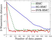
(a) $d=10,n=50$

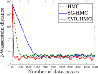
(b) $d=10,n=100$

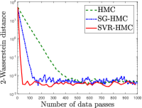
(c) $d=10,n=1000$

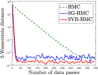
(d) $d=10,n=5000$

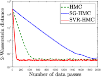
(e) $d=50,n=50$

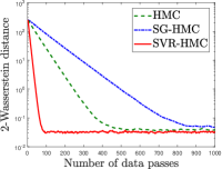
(f) $d=50,n=100$

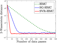
(g) $d=50,n=1000$

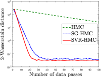
(h) $d=50,n=5000$

Figure 1: Numerical results for synthetic data, where we compare $3$ different algorithms, and show their convergence performance in $2$-Wasserstein distance. (a)-(h) represent for different dimensions $d$ and sample sizes $n$.

5 Experiments

In this section, we compare the proposed algorithm (SVR-HMC) with the state-of-the-art MCMC algorithms for Bayesian learning. To compare the convergence rates for different MCMC algorithms, we conduct the experiments on both synthetic data and real data.

We compare our algorithm with SGLD (Welling & Teh, 2011), VR-SGLD (Reddi et al., 2016), HMC (Cheng & Bartlett, 2017) and SG-HMC (Cheng & Bartlett, 2017).

5.1 Simulation Based on Synthetic Data

On the synthetic data, we construct each component function to be $f_{i}(\mathbf{x})=(\mathbf{x}-\bm{a}_{i})^{\top}\bm{\Sigma}(\mathbf{x}-\bm{a}_{i})/2$, where $\mathbf{a}_{i}$ is a Gaussian random vector drawn from distribution $\mathcal{N}(2,4\times\mathbf{I}_{d\times d})$, and $\bm{\Sigma}$ is a positive definite symmetric matrix with maximum eigenvalue $L=3/2$ and minimum eigenvalue $\mu=2/3$. Note that each random vector $\bm{a}_{i}$ leads to a particular component function $f_{i}(\mathbf{x})$. Then it can be observed that the target density $\pi\propto\exp\big{(}1/n\sum_{i=1}^{n}f_{i}(\mathbf{x})\big{)}=\exp\big{(}(\mathbf{x}-\bar{\bm{a}})^{\top}\bm{\Sigma}(\mathbf{x}-\bar{\bm{a}})/2\big{)}$ is a multivariate Gaussian distribution with mean $\bar{\bm{a}}=1/n\sum_{i=1}^{n}\bm{a}_{i}$ and covariance matrix $\bm{\Sigma}$. Moreover, the negative log density $f(\mathbf{x})$ is $L$-smooth and $\mu$-strongly convex.

In our simulation, we investigate different dimension $d$ and number of component functions $n$, and show the 2-Wasserstein distance between the target distribution $\pi$ and that of the output from different algorithms with respect to the number of data passes. In order to estimate the $2$-Wasserstein distance between the distribution of each iterate and the target one, we repeat all algorithms for $20,000$ times and obtain $20,000$ random samples for each algorithm in each iteration. In Figure 1, we present the convergence results for three HMC based algorithms (HMC, SG-HMC and SVR-HMC). It is evident that SVR-HMC performs the best among these three algorithms when $n$ is not large enough, and its performance becomes close to that of SG-HMC when the number of component function is increased. This phenomenon is well-aligned with our theoretical analysis, since the gradient complexity of our algorithm can be worse than SG-HMC when the sample size $n$ is extremely large.

5.2 Bayesian Logistic Regression for Classification

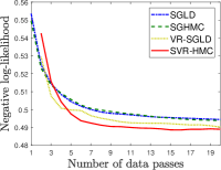
(a) pima

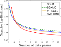
(b) a3a

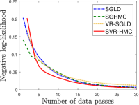
(c) gisette

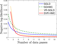
(d) mushroom

Figure 2: Comparison of different algorithms for Bayesian logistic regression, where $y$ axis shows the negative log-likelihood on the test data, and $y$ axis is the number of data passess. (a)-(d) correspond to $4$ datasets.

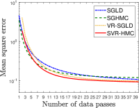
(a) geographical

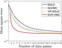
(b) noise

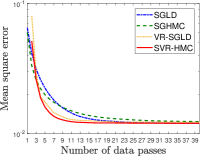
(c) parkinson

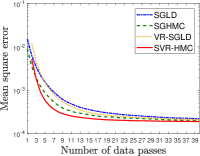
(d) toms

Figure 3: Comparison of different algorithms for Bayesian linear regression, where $y$ axis is the mean square errors on the test data, and $x$ axis is the number of data passess. (a)-(d) correspond to $4$ datasets.

Table 2: Summary of datasets for Bayesian classification

Dataset	pima	a3a	gisette	mushroom
$n$ (training)	384	3185	6000	4062
$n$ (test)	384	29376	1000	4062
$d$	8	122	5000	112

Table 3: Test error of different algorithms for Bayesian classification after $10$ entire data passes on $4$ datasets

Dateset	pima	a3a	gisette	mushroom
SGLD	$0.2314\pm 0.0044$	$0.1594\pm 0.0018$	$0.0098\pm 0.0009$	$(6.647+2.251)\times 10^{-4}$
SGHMC	$0.2306\pm 0.0079$	$0.1591\pm 0.0044$	$0.0096\pm 0.0006$	$(5.916\pm 2.734)\times 10^{-4}$
VR-SGLD	$0.2299+0.0056$	$0.1572\pm 0.0012$	$0.0105\pm 0.0006$	$(7.755\pm 3.231)\times 10^{-4}$
SVR-HMC	$0.2289\pm 0.0043$	$0.1570\pm 0.0019$	$0.0093\pm 0.0011$	$(6.278\pm 3.149)\times 10^{-4}$

Now, we apply our algorithm to the Bayesian logistic regression problems. In logistic regression, given $n$ i.i.d. examples $\{\mathbf{a}_{i},y_{i}\}_{i=1,\dots,n}$, where $\mathbf{a}_{i}\in\mathbb{R}^{d}$ and $y_{i}\in\{0,1\}$ denote the features and binary labels respectively, the probability mass function of $y_{i}$ given the feature $\mathbf{a}_{i}$ is modelled as $p(y_{i}|\mathbf{a}_{i},\mathbf{x})=1/\big{(}1+e^{-y_{i}\mathbf{x}^{\top}\bm{a}_{i}}\big{)}$, where $\mathbf{x}\in\mathbb{R}^{d}$ is the regression parameter. Considering the prior $p(\mathbf{x})=\mathcal{N}(\mathbf{0},\lambda^{-1}\mathbf{I})$, the posterior distribution takes the form

$$p(\mathbf{x}|\bm{A},\bm{Y})\propto p(\bm{Y}|\bm{A},\mathbf{x})p(\mathbf{x})=\prod_{i=1}^{n}p(y_{i}|\mathbf{a}_{i},\mathbf{\beta})p(\mathbf{x}).$$

where $\bm{A}=[\mathbf{a}_{1},\mathbf{a}_{2},\ldots,\mathbf{a}_{n}]^{\top}$ and $\bm{Y}=[y_{1},y_{2},\ldots,y_{n}]^{\top}$. The posterior distribution can be written as $p(\mathbf{x}|\bm{A},\bm{Y})\propto e^{-\sum_{i=1}^{n}f_{i}(\mathbf{x})}$, where each $f_{i}(\mathbf{x})$ is in the following form

$$f_{i}(\mathbf{x})=n\log\big{(}1+\exp(-y_{i}\mathbf{x}^{\top}\mathbf{a}_{i})\big{)}+\lambda/2\|\mathbf{x}\|_{2}^{2}.$$

We use four binary classification datasets from Libsvm (Chang & Lin, 2011) and UCI machine learning repository (Lichman, 2013), which are summarized in Table LABEL:table:dataset. Note that pima and mushroom do not have test data in their original version, and we split them into $50\%$ for training and $50\%$ for test. Following Welling & Teh (2011); Chen et al. (2014, 2015), we report the sample path average and discard the first $50$ iterations as burn-in. It is worth noting that we observe similar convergence comparison of different algorithms for larger burn-in period $(=10^{4})$. We run each algorithm $20$ times and report the averaged results for comparison. Note that variance reduction based algorithms (i.e., VR-SGLD and SVR-HMC) require the first data pass to compute one full gradient. Therefore, in Figure 2, plots of VR-SGLD and VRHMC start from the second data pass while plots of SGLD and SGHMC start from the first data pass. It can be clearly seen that our proposed algorithm is able to converge faster than SGLD and SG-HMC on all datasets, which validates our theoretical analysis of the convergence rate. In addition, although there is no existing non-asymptotic theoretical guarantee for VR-SGLD when the target distribution is strongly log-concave, from Figure 2, we can observe that SVR-HMC also outperforms VR-SGLD on these four datasets, which again demonstrates the superior performance of our algorithm. This clearly shows the advantage of our algorithm for Bayesian learning.

5.3 Bayesian Linear Regression

Table 4: Summary of datasets for Bayesian linear regression

Dataset	geographical	noise	parkinson	toms
$n$	1059	1503	5875	45730
$d$	69	5	21	96

We also apply our algorithm to Bayesian linear regression, and make comparison with the baseline algorithms. Similar to Bayesian classification, given i.i.d. examples $\{\mathbf{a}_{i},y_{i}\}_{i=1,\dots,n}$ with $y_{i}\in\mathbb{R}$, the likelihood of Bayessian linear regression is $p(y_{i}|\mathbf{a}_{i},\mathbf{x})=\mathcal{N}(\mathbf{x}^{\top}\mathbf{a}_{i},\sigma_{a}^{2})$ and the prior is $\mathcal{N}(\mathbf{0},\lambda^{-1}\mathbf{I})$. We use $4$ datasets, which are summarized in Table LABEL:table:dataset2. In our experiment, we set $\sigma_{a}^{2}=1$ and $\lambda=1$, and conduct the normalization of the original data. In addition, we split each dataset into training and test data evenly. Similarly, we compute the sample path average while treating the first $50$ iterates as burn in. We report the mean square errors on the test data on these $4$ datasets in Figure 3 for different algorithms. It is evident that our algorithm is faster than all the other baseline algorithms on all the datasets, which further illustrates the advantage of our algorithm for Bayesian learning.

6 Conclusions and Future work

We propose a stochastic variance reduced Hamilton Monte Carlo (HMC) method, for sampling from a smooth and strongly log-concave distribution. We show that, to achieve $\epsilon$ accuracy in 2-Wasserstein distance, our algorithm enjoys a faster rate of convergence and better gradient complexity than state-of-the-art HMC and stochastic gradient HMC methods in a wide regime. We also extend our algorithm for sampling from smooth and general log-concave distributions. Experiments on both synthetic and real data verified the superior performance of our algorithm. In the future, we will extend our algorithm to non-log-concave distributions and study the symplectic integration techniques such as Leap-frog integration for Bayesian posterior sampling.

Appendix A Proof of Main Theory

In this section, we present our theoretical analysis of the proposed SVR-HMC algorithm. Before we present the proof of our main theorem, we introduce some notations for the ease of our presentation. We use notation ${\mathcal{S}}_{\eta}$ to denote the one-step SVR-HMC update in (3.1) with step size $\eta$, i.e., $\mathbf{x}_{k+1}={\mathcal{S}}_{\eta}\mathbf{x}_{k}$ and $\mathbf{v}_{k+1}={\mathcal{S}}_{\eta}\mathbf{v}_{k}$. Similarly, We define an operator $\mathcal{G}_{\eta}$ which also performs one step update with step size $\eta$, but replaces the semi-stochastic gradient in (3.1) with the full gradient. Specifically, we have

$$\begin{split}\mathcal{G}_{\eta}\mathbf{v}_{k}&=\mathbf{v}_{k}-\gamma\eta\mathbf{v}_{k}-\eta u\nabla f(\mathbf{x}_{k})+\bm{\epsilon}_{k}^{v},\\ \mathcal{G}_{\eta}\mathbf{x}_{k}&=\mathbf{x}_{k}+\eta\mathbf{v}_{k}+\bm{\epsilon}_{k}^{x},\end{split}$$ (A.1)

for any $\mathbf{x}_{k},\mathbf{v}_{k}\in\mathbb{R}^{d}$, where $\bm{\epsilon}_{k}^{v}$ and $\bm{\epsilon}_{k}^{x}$ are the same as defined in Algorithm 1. Next, we define an operator $\mathcal{L}_{\eta}$ which represents the integration over a time interval of length $\eta$ on the continuous dynamics (1.3). Specifically, for any starting point $\bm{V}_{0}$ and $\bm{X}_{0}$, integrating (1.3) over time interval $(0,\eta)$ yields the following equations:

$$\bm{V}_{t} =\mathcal{L}_{t}\bm{V}_{0}=\bm{V}_{0}e^{-\gamma t}-u\bigg{(}\int_{0}^{t}e^{-\gamma(t-s)}\nabla f(\bm{X}_{t})\text{d}s\bigg{)}+\sqrt{2\gamma u}\int_{0}^{t}e^{-\gamma(t-s)}\text{d}\bm{B}_{s},$$ (A.2)

$$\bm{X}_{t} =\mathcal{L}_{t}\bm{X}_{0}=\bm{X}_{0}+\int_{0}^{t}\bm{V}_{s}\text{d}s.$$ (A.3)

(A.2) and (A.3) give out an implicit solution of dynamics (1.3), which can be easily verified by taking derivatives of these two equations (Cheng et al., 2017). The following lemma characterizes the mean value and covariance of the Brownian motion terms.

Lemma A.1.

(Cheng et al., 2017) The additive Brownian motion in (A.2), denoted by $\bm{\epsilon}^{v}=\sqrt{2\gamma u}\int_{0}^{t}e^{-\gamma(t-s)}d\bm{B}_{s}$, has mean $\mathbf{0}$ and covariance matrix

$$\mathbb{E}[\bm{\epsilon}^{v}(\bm{\epsilon}^{v})^{\top}]=2\gamma u\mathbb{E}\bigg{[}\int_{0}^{t}e^{-\gamma(t-s)}\text{d}\bm{B}_{s}\int_{0}^{t}e^{-\gamma(t-s)}\text{d}\bm{B}_{s}^{\top}\bigg{]}=u(1-e^{-2\gamma t})\cdot\mathbf{I}_{d\times d}.$$

Note that there also exists a hidden Brownian motion term in (A.3), which comes from the velocity $\bm{V}_{s}$, denoted by $\bm{\epsilon}^{x}=\sqrt{2\gamma u}\int_{0}^{t}\int_{0}^{s}e^{-\gamma(s-r)}\text{d}\bm{B}_{r}\text{d}t$, having mean $\mathbf{0}$ and covariance matrix

$$\mathbb{E}[\bm{\epsilon}^{x}(\bm{\epsilon}^{x})^{\top}]=2\gamma u\mathbb{E}\bigg{[}\int_{0}^{t}\int_{0}^{s}e^{-\gamma(s-r)}\text{d}B_{r}\text{d}s\int_{0}^{t}\int_{0}^{s}e^{-\gamma(s-r)}\text{d}\bm{B}_{r}^{\top}\text{d}s\bigg{]}=\frac{u}{\gamma^{2}}(2\gamma t+4e^{-\gamma t}-e^{-2\gamma t}-3)\cdot\mathbf{I}_{d\times d}.$$

In addition, $\bm{\epsilon}^{v}$ and $\bm{\epsilon}^{x}$ have the following cross-covariance

$$\mathbb{E}[\bm{\epsilon}^{v}(\bm{\epsilon}^{x})^{\top}]=2\gamma u\mathbb{E}\bigg{[}\int_{0}^{t}e^{-\gamma(t-s)}\text{d}\bm{B}_{s}\int_{0}^{t}\int_{0}^{s}e^{-\gamma(s-r)}\text{d}\bm{B}_{r}^{\top}\text{d}s\bigg{]}=\frac{u}{\gamma}(1-2e^{-\gamma t}+e^{-2\gamma t})\cdot\mathbf{I}_{d\times d}.$$

Recall the independent Gaussian random vectors $\bm{\epsilon}_{k}^{v}$ and $\bm{\epsilon}_{k}^{x}$ used in each iteration of Algorithm 1. They all have zero mean and the covariance matrices defined in (3) have exactly the same form with the covariance matrices in Lemma A.1 when $t=\eta$. Due to this property, we will use a synchronous coupling technique that ensures the Gaussian random vectors in each one-step update of the discrete algorithm, i.e., ${\mathcal{S}}_{\eta}\mathbf{x}$ and ${\mathcal{S}}_{\eta}\mathbf{v}$, are exactly the same additive Brownian motion terms in the one-step integration of the continuous dynamics $\mathcal{L}_{\eta}\mathbf{x}$ and $\mathcal{L}_{\eta}\mathbf{v}$. The shared Brownian motions between ${\mathcal{S}}_{\eta}\mathbf{v}$ and $\mathcal{L}_{\eta}\mathbf{v}$ (${\mathcal{S}}_{\eta}\mathbf{x}$ and $\mathcal{L}_{\eta}\mathbf{x}$) are pivotal to our analysis. Similar coupling techniques are also used in Eberle et al. (2017); Cheng et al. (2017).

A.1 Proof of Theorem 4.3

We first lay down some technical lemmas that are useful in our proof. The first lemma characterizes the discretization error between the full gradient-based HMC update in (A.1) and the solutions of continuous Hamiltonian dynamics (1.3).

Lemma A.2.

Under Assumptions 4.1 and 4.2, consider one-step discrete update (A.1) and Langevin diffusion (A.2)-(A.3) starting from point $(\mathbf{x}_{k},\mathbf{v}_{k})$. Then the discretization error for velocity and position are bounded by

$$\mathbb{E}[\|\mathcal{G}_{\eta}\mathbf{x}_{k}-\mathcal{L}_{\eta}\mathbf{x}_{k}\|_{2}^{2}] \leq\eta^{4}\bigg{[}\bigg{(}\frac{2\gamma^{2}+2uL}{3}\bigg{)}U_{v}+\frac{4u^{2}L}{3}U_{f}+\frac{8u^{2}L\gamma d\eta}{3}\bigg{]}\triangleq D_{1}\eta^{4},$$

$$\mathbb{E}[\|\mathcal{G}_{\eta}\mathbf{v}_{k}-\mathcal{L}_{\eta}\mathbf{v}_{k}\|_{2}^{2}] \leq\eta^{4}\bigg{[}\Big{(}\frac{3\gamma^{4}}{4}+u^{2}L^{2}\Big{)}U_{v}+\Big{(}\frac{3u^{2}\gamma^{2}L}{2}+4u^{3}L^{2}\Big{)}U_{f}+4u^{3}L^{2}\eta\gamma d\bigg{]}\triangleq D_{2}\eta^{4},$$

where parameters $U_{v}$ and $U_{f}$ are in the order of $O(d/\mu)$ and $O(d\kappa)$ respectively.

The difference between our SVR-HMC update and the full gradient-based HMC update in (A.1) can be characterized by the following lemma.

Lemma A.3.

Under Assumptions 4.1 and 4.2, for any $\mathbf{x}_{k},\mathbf{v}_{k}\in\mathbb{R}^{d}$, we have

$$\mathbb{E}[\|{\mathcal{S}}_{\eta}\mathbf{x}_{k}-\mathcal{G}_{\eta}\mathbf{x}_{k}\|_{2}^{2}] =0,$$ (A.4)

$$\mathbb{E}[\|{\mathcal{S}}_{\eta}\mathbf{v}_{k}-\mathcal{G}_{\eta}\mathbf{v}_{k}\|_{2}^{2}] \leq 2\eta^{4}m^{2}u^{2}L^{2}(U_{v}+\gamma ud)\triangleq D_{3}u^{2}L^{2}m^{2}\eta^{4}.$$ (A.5)

The following lemma shows the contraction property for the diffusion operator in terms of the coupled $\ell_{2}$ norm.

Lemma A.4.

(Cheng et al., 2017) Under Assumptions 4.1 and 4.2, let $\mathbf{z}=(\mathbf{x}^{\top},(\mathbf{x}+\mathbf{v})^{\top})^{\top}\in\mathbb{R}^{2d}$ and $\mathcal{L}_{t}\mathbf{z}=((\mathcal{L}_{t}\mathbf{x})^{\top},(\mathcal{L}_{t}\mathbf{x}+\mathcal{L}_{t}\mathbf{v})^{\top})^{\top}$. Set $\gamma=2$ and $u=1/L$ in (A.2)-(A.3). Starting from two different points $\mathbf{z}_{1}$ and $\mathbf{z}_{2}$, the continuous-time dynamics after time $t$ satisfy

$$\mathbb{E}[\|\mathcal{L}_{t}\mathbf{z}_{1}-\mathcal{L}_{t}\mathbf{z}_{2}\|_{2}^{2}]\leq e^{-t/\kappa}\mathbb{E}[\|\mathbf{z}_{1}-\mathbf{z}_{2}\|_{2}^{2}],$$

where the diffusion operators on $\mathbf{z}_{1}$ and $\mathbf{z}_{2}$ share the same Brownian motion, and $\kappa=L/\mu$ denotes the condition number.

For the operators $\mathcal{L}_{\eta}$, we denote $\mathcal{L}_{\eta}^{k}\mathbf{x}=\mathcal{L}_{\eta}\circ\mathcal{L}_{\eta}\circ\cdots\circ\mathcal{L}_{\eta}\mathbf{x}$ as the result after $\mathcal{L}_{\eta}$ operates $k$ times starting at $\mathbf{x}$. We have the following lemma which is useful to characterize the distance $\mathbb{E}[\|\mathbf{z}_{k}-\mathcal{L}_{\eta}^{k}\mathbf{z}^{\pi}\|_{2}^{2}]$ based on some recursive arguments, where $\mathbf{z}^{\pi}=\big{(}(\mathbf{x}^{\pi})^{\top},(\mathbf{x}^{\pi}+\mathbf{v}^{\pi})^{\top}\big{)}^{\top}$.

Lemma A.5.

(Dalalyan & Karagulyan, 2017) Let $A$, $B$ and $C$ be given non-negative numbers such that $A\in(0,1)$. Assume that the sequence of non-negative numbers $\{x_{k}\}_{k=0,1,2,\dots}$ satisfies the recursive inequality

$$x_{k+1}^{2}\leq[(1-A)x_{k}+C]^{2}+B^{2},$$

for every integer $k\geq 0$. Then, for all integers $k\geq 0$,

$$x_{k}\leq(1-A)^{k}x_{0}+\frac{C}{A}+\frac{B}{\sqrt{A}}.$$

Lemma A.6.

For any two random vectors $\bm{X},\bm{Y}\in\mathbb{R}^{d}$, the following holds

$$\mathbb{E}[\|\bm{X}+\bm{Y}\|_{2}^{2}]\leq\bigg{(}\sqrt{\mathbb{E}[\|\bm{X}\|_{2}^{2}]}+\sqrt{\mathbb{E}[\|\bm{Y}\|_{2}^{2}]}\bigg{)}^{2}.$$

Based on all the above lemmas, we are now ready to prove Theorem 4.3.

Proof of Theorem 4.3.

Let $\mathbf{z}^{\pi}$ denote the random variable satisfying distribution $\pi_{\mathbf{z}}$, then we have

$$\mathbb{E}[\|\mathbf{z}_{k+1}-\mathcal{L}_{\eta}^{k+1}\mathbf{z}^{\pi}\|_{2}^{2}] =\mathbb{E}[\|\mathbf{z}_{k+1}-\mathcal{G}_{\eta}\mathbf{z}_{k}+\mathcal{G}_{\eta}\mathbf{z}_{k}-\mathcal{L}_{\eta}^{k+1}\mathbf{z}^{\pi}\|_{2}^{2}]$$

$$=\mathbb{E}[\|\mathbf{z}_{k+1}-\mathcal{G}_{\eta}\mathbf{z}_{k}\|_{2}^{2}+2\langle\mathbf{z}_{k+1}-\mathcal{G}_{\eta}\mathbf{z}_{k},\mathcal{G}_{\eta}\mathbf{z}_{k}-\mathcal{L}_{\eta}^{k+1}\mathbf{z}^{\pi}\rangle+\|\mathcal{G}_{\eta}\mathbf{z}_{k}-\mathcal{L}_{\eta}^{k+1}\mathbf{z}^{\pi}\|_{2}^{2}]$$

$$=\mathbb{E}[\|\mathbf{z}_{k+1}-\mathcal{G}_{\eta}\mathbf{z}_{k}\|_{2}^{2}+\|\mathcal{G}_{\eta}\mathbf{z}_{k}-\mathcal{L}_{\eta}^{k+1}\mathbf{z}^{\pi}\|_{2}^{2}],$$ (A.6)

where the last equality follows from the fact that $\mathbb{E}\big{[}\langle\mathbf{z}_{k+1}-\mathcal{G}_{\eta}\mathbf{z}_{k},\mathcal{G}_{\eta}\mathbf{z}_{k}-\mathcal{L}_{\eta}^{k+1}\mathbf{z}^{\pi}\rangle\big{]}=\mathbb{E}\big{[}\mathbb{E}_{i_{k}}[\langle\mathbf{z}_{k+1}-\mathcal{G}_{\eta}\mathbf{z}_{k},\mathcal{G}_{\eta}\mathbf{z}_{k}-\mathcal{L}_{\eta}^{k+1}\mathbf{z}^{\pi}\rangle]\big{]}=\mathbf{0}$ and $\mathbb{E}_{i_{k}}[\mathbf{z}_{k+1}]=\mathcal{G}_{\eta}\mathbf{z}_{k}$. Note that $\mathbf{z}_{k+1}=(\mathbf{x}_{k+1}^{\top},(\mathbf{x}_{k+1}+\mathbf{v}_{k+1})^{\top})^{\top}$, thus

$$\mathbb{E}[\|\mathbf{z}_{k+1}-\mathcal{G}_{\eta}\mathbf{z}_{k}\|_{2}^{2} =\mathbb{E}[\|\mathbf{x}_{k+1}-\mathcal{G}_{\eta}\mathbf{x}_{k}\|_{2}^{2}+\mathbb{E}[\|\mathbf{x}_{k+1}+\mathbf{v}_{k+1}-\mathcal{G}_{\eta}(\mathbf{x}_{k}+\mathbf{v}_{k})\|_{2}^{2}$$

$$=\mathbb{E}[\|\mathbf{v}_{k+1}-\mathcal{G}_{\eta}\mathbf{v}_{k}\|_{2}^{2}$$ (A.7)

$$\leq D_{3}m^{2}\eta^{4},$$ (A.8)

where the second equality follows from $\mathbf{x}_{k+1}=\mathcal{G}_{\eta}\mathbf{x}_{k}$, the inequality follows from Lemma A.3 and the fact that $uL=1$. The second term on the R.H.S of (A.1) can be further bounded as follows,

$$\mathbb{E}[\|\mathcal{G}_{\eta}\mathbf{z}_{k}-\mathcal{L}_{\eta}^{k+1}\mathbf{z}^{\pi}\|_{2}^{2}] =\mathbb{E}[\|\mathcal{G}_{\eta}\mathbf{z}_{k}-\mathcal{L}_{\eta}\mathbf{z}_{k}+\mathcal{L}_{\eta}\mathbf{z}_{k}-\mathcal{L}_{\eta}^{k+1}\mathbf{z}^{\pi}\|_{2}^{2}]$$

$$\leq\bigg{(}\sqrt{\mathbb{E}[\|\mathcal{G}_{\eta}\mathbf{z}_{k}-\mathcal{L}_{\eta}\mathbf{z}_{k}\|_{2}^{2}]}+\sqrt{\mathbb{E}[\|\mathcal{L}_{\eta}\mathbf{z}_{k}-\mathcal{L}_{\eta}^{k+1}\mathbf{z}^{\pi}\|_{2}^{2}]}\bigg{)}^{2}$$

$$\leq\bigg{(}\sqrt{\mathbb{E}[\|\mathcal{G}_{\eta}\mathbf{z}_{k}-\mathcal{L}_{\eta}\mathbf{z}_{k}\|_{2}^{2}]}+e^{-\eta/(2\kappa)}\sqrt{\mathbb{E}[\|\mathbf{z}_{k}-\mathcal{L}_{\eta}^{k}\mathbf{z}^{\pi}\|_{2}^{2}]}\bigg{)}^{2},$$ (A.9)

where the first inequality holds due to Lemma A.6 and the second inequality follows from Lemma A.4. We further have

$$\sqrt{\mathbb{E}[\|\mathcal{G}_{\eta}\mathbf{z}_{k}-\mathcal{L}_{\eta}\mathbf{z}_{k}\|_{2}^{2}]} =\sqrt{\mathbb{E}[\|\mathcal{G}_{\eta}(\mathbf{v}_{k}+\mathbf{x}_{k})-\mathcal{L}_{\eta}(\mathbf{v}_{k}+\mathbf{x}_{k})\|_{2}^{2}]+\mathbb{E}[\|\mathcal{G}_{\eta}\mathbf{x}_{k}-\mathcal{L}_{\eta}\mathbf{x}_{k}\|_{2}^{2}]}$$

$$\leq\sqrt{\mathbb{E}[\|\mathcal{G}_{\eta}(\mathbf{v}_{k}+\mathbf{x}_{k})-\mathcal{L}_{\eta}(\mathbf{v}_{k}+\mathbf{x}_{k})\|_{2}^{2}}+\sqrt{\mathbb{E}[\|\mathcal{G}_{\eta}\mathbf{x}_{k}-\mathcal{L}_{\eta}\mathbf{x}_{k}\|_{2}^{2}]}$$

$$\leq 2\sqrt{\mathbb{E}[\|\mathcal{G}_{\eta}\mathbf{x}_{k}-\mathcal{L}_{\eta}\mathbf{x}_{k}\|_{2}^{2}]}+\sqrt{\mathbb{E}[\|\mathcal{G}_{\eta}\mathbf{v}_{k}-\mathcal{L}_{\eta}\mathbf{v}_{k}\|_{2}^{2}]}$$ (A.10)

$$\leq 2\sqrt{D_{1}}\eta^{2}+\sqrt{D_{2}}\eta^{2},$$ (A.11)

where the first inequality is due to $\sqrt{a+b}\leq\sqrt{a}+\sqrt{b}$, the second inequality is due to (B.3) and the last inequality comes from Lemma A.2. Here $D_{1}$, $D_{2}$ are constants which are both in the order of $O(d/\mu)$. Denote $w_{k+1}^{2}=\mathbb{E}[\|\mathbf{z}_{k+1}-\mathcal{L}_{\eta}^{k+1}\mathbf{z}^{\pi}\|_{2}^{2}]$. Submitting (A.8), (A.1) and (A.11) into (A.1) yields

$$w_{k+1}^{2} \leq\Big{(}e^{-\eta/(2\kappa)}w_{k}+2\sqrt{D_{1}}\eta^{2}+\sqrt{D_{2}}\eta^{2}\Big{)}^{2}+D_{3}m^{2}\eta^{4}.$$ (A.12)

Then, by Lemma A.5, $w_{k}$ can be bounded by

$$w_{k} \leq e^{-k\eta/(2\kappa)}w_{0}+\frac{2\sqrt{D_{1}}\eta^{2}+\sqrt{D_{2}}\eta^{2}}{1-e^{-\eta/(2\kappa)}}+\frac{\sqrt{D_{3}}m\eta^{2}}{\sqrt{1-e^{-\eta/(2\kappa)}}}.$$

Note that the above results rely on the shared Brownian motion in the discrete update and continuous Langevin diffusion, i.e., we assume identical Brownian motion sequences are used in the updates $\mathbf{z}_{k}={\mathcal{S}}_{\eta}^{k}\mathbf{z}_{0}$ and $\mathcal{L}_{\eta}^{k}\mathbf{z}^{\pi}$. Since $\mathbf{z}^{\pi}$ satisfies the stationary distribution $\pi_{\mathbf{z}}$, $\mathcal{L}_{\eta}^{k}\mathbf{z}^{\pi}$ satisfies $\pi_{\mathbf{z}}$ as well. According to the definition of $2$-Wasserstein distance, we have

$$\mathcal{W}_{2}\big{(}P(\mathbf{z}_{k}),\pi_{\mathbf{z}}\big{)} =\bigg{(}\inf_{\zeta\in\Gamma(\mathbf{z}_{k},\mathcal{L}_{\eta}^{k}\mathbf{z}^{\pi})}\int_{\mathbb{R}^{d}\times\mathbb{R}^{d}}\|\mathbf{z}_{k}-\mathcal{L}_{\eta}^{k}\mathbf{z}^{\pi}\|_{2}^{2}\text{d}\zeta(\mathbf{z}_{k},\mathcal{L}_{\eta}^{k}\mathbf{z}^{\pi})\bigg{)}^{1/2}$$

$$\leq\sqrt{\mathbb{E}[\|\mathbf{z}_{k}-\mathcal{L}_{\eta}^{k}\mathbf{z}^{\pi}\|_{2}^{2}]}$$

$$=w_{k},$$

which further implies that

$$\mathcal{W}_{2}\big{(}P(\mathbf{z}_{K}),\pi_{\mathbf{z}}\big{)} \leq w_{K}\leq e^{-K\eta/(2\kappa)}w_{0}+\frac{2\sqrt{D_{1}}\eta^{2}+\sqrt{D_{2}}\eta^{2}}{1-e^{-\eta/(2\kappa)}}+\frac{\sqrt{D_{3}}m\eta^{2}}{\sqrt{1-e^{-\eta/(2\kappa)}}}.$$ (A.13)

Let $K\eta=T$, and note that $1-e^{-\eta/(2\kappa)}\geq\eta/(4\kappa)$ when assuming $0<\eta/\kappa\leq 1$. Therefore, we have

$$\mathcal{W}_{2}\big{(}P(\mathbf{z}_{K}),\pi_{\mathbf{z}}\big{)} \leq w_{K}\leq e^{-T/(2\kappa)}w_{0}+4\eta\kappa(2\sqrt{D_{1}}+\sqrt{D_{2}})+2\sqrt{\kappa D_{3}}m\eta^{3/2}.$$ (A.14)

Moreover, note that

$$\mathcal{W}_{2}\big{(}P(\mathbf{x}_{K}),\pi\big{)} =\mathbb{E}_{\Gamma(\mathbf{x}_{K},\mathbf{x}^{\pi})}[\|\mathbf{x}_{K}-\mathbf{x}^{\pi}\|_{2}^{2}]$$

$$\leq\mathbb{E}_{\Gamma(\mathbf{x}_{K},\mathbf{v}_{K},\mathbf{x}^{\pi},\mathbf{v}^{\pi})}[\|\mathbf{x}_{K}-\mathbf{x}^{\pi}\|_{2}^{2}+\|\mathbf{x}_{K}+\mathbf{v}_{K}-\mathbf{x}^{\pi}-\mathbf{v}^{\pi}\|_{2}^{2}]$$

$$=\mathcal{W}_{2}\big{(}P(\mathbf{z}_{K}),\pi_{\mathbf{z}}\big{)}.$$

Substituting the above into (A.14) directly yields the argument in Theorem 4.3. ∎

A.2 Proof of Corollary 4.5

Now we present the calculation of gradient complexity of our algorithm.

We first present the following Lemma that characterizes the expectation $\mathbb{E}[\|\mathbf{x}^{\pi}-\mathbf{x}^{*}\|]$, where $\mathbf{x}^{*}=\arg\min_{\mathbf{x}}f(\mathbf{x})$ is the global minimizer of function $f$.

Lemma A.7 (Proposition 1 in Durmus & Moulines (2016b)).

Let $\mathbf{x}^{*}=\arg\min_{\mathbf{x}}f(\mathbf{x})$ denote the global minimizer of function $f$, and $\mathbf{x}^{\pi}$ be the random vector satisfying distribution $\pi\propto e^{-f(\mathbf{x})}$, the following holds,

$$\mathbb{E}[\|\mathbf{x}^{\pi}-\mathbf{x}^{*}\|_{2}^{2}]\leq\frac{d}{\mu}.$$

Then we are going to prove Corollary 4.5.

Proof of Corollary 4.5.

We first let $w_{0}e^{-T/2\kappa}=\epsilon/3$, which implies that $T=2\kappa\log(3w_{0}/\epsilon)$. Note that $\mathbf{x}^{*}$ is the minimizer of $f$ and by assumption we have $\|\mathbf{x}_{0}-\mathbf{x}^{*}\|_{2}\leq R$. Recall the definition of $w_{k}$, we have

$$w_{0} =\mathbb{E}[\|\mathbf{x}_{0}-\mathbf{x}^{\pi}\|_{2}^{2}]=\mathbb{E}[\|\mathbf{x}_{0}-\mathbf{x}^{*}+\mathbf{x}^{*}-\mathbf{x}^{\pi}\|_{2}^{2}]\leq 2\mathbb{E}[\|\mathbf{x}^{\pi}-\mathbf{x}^{*}\|_{2}^{2}]+2\|\mathbf{x}_{0}-\mathbf{x}^{*}\|_{2}^{2}\leq\frac{2d}{\mu}+2R,$$

where the last inequality comes from Lemma A.7. Then we obtain $T=\widetilde{O}(\kappa)$, where $\widetilde{O}(\cdot)$ notation hides the logarithmic term of $\epsilon$, $d$, $\mu$ and $R$. We then rewrite (A.14) as follow,

$$\mathcal{W}_{2}\big{(}P(\mathbf{z}_{K}),\pi_{\mathbf{z}}\big{)} \leq e^{-T/(2\kappa)}w_{0}+\widetilde{C}_{2}\eta+\widetilde{C}_{3}m\eta^{3/2},$$ (A.15)

where $\widetilde{C}_{2}=O(\kappa(d/\mu)^{1/2})$ and $\widetilde{C}_{3}=O\big{(}(\kappa d/\mu)^{1/2}\big{)}$. We then let

$$\widetilde{C}_{2}\eta=\frac{\epsilon}{3},\quad\mbox{and}\quad\widetilde{C}_{3}m\eta^{3/2}=\frac{\epsilon}{3},$$

and solve for $\eta$, which leads to

$$\eta=\min\bigg{\{}\frac{\epsilon}{3\widetilde{C}_{2}},\frac{\epsilon^{2/3}}{(3\widetilde{C}_{3}m)^{2/3}}\bigg{\}}.$$

Thus, the total iteration number satisfies

$$K=\frac{T}{\eta}\leq\frac{3T\widetilde{C}_{2}}{\epsilon}+\frac{T(3\widetilde{C}_{3}m)^{2/3}}{\epsilon^{2/3}}.$$

In terms of gradient complexity, we have

$$T_{g}=K+n\bigg{(}1\vee\frac{K}{m}\bigg{)}\leq K+\frac{Kn}{m}+n.$$

Substituting $\widetilde{C}_{2}$, $\widetilde{C}_{3}$, $T$ into the above equation, and let $m=n$, we obtain

$$T_{g}\leq 2K+n=\widetilde{O}\bigg{(}\frac{\kappa^{2}(d/\mu)^{1/2}}{\epsilon}+\frac{\kappa^{4/3}(d/\mu)^{1/3}n^{2/3}}{\epsilon^{2/3}}+n\bigg{)}.$$ (A.16)

When $\mu$ and $L$ appear individually, they can be treated as constants. Thus we arrive at the result in Corollary 4.5. ∎

A.3 Proof of Theorem 4.8

In this section, we prove the convergence result of SVR-HMC for sampling from a general log-concave distribution. Note that for a $\mu$-strongly log-concave distribution $\pi\propto e^{-f}$, it must satisfy a logarithmic Sobolev inequality with constant $C_{LS}=1/\mu$ (Raginsky et al., 2017). We first present the following two useful lemmas.

Lemma A.8.

(Dalalyan, 2014) Let $f$ and $\bar{f}$ be two functions such that $f(\mathbf{x})\leq\bar{f}(\mathbf{x})$ for all $\mathbf{x}\in\mathbb{R}^{d}$, suppose $e^{-f}$ and $e^{-\bar{f}}$ are both integratable. Then the Kullback-Leibler (KL) divergence between distribution $\pi\propto e^{-f}$ and $\bar{\pi}\propto e^{-\bar{f}}$ satisfies

$$\mbox{KL}(\pi||\bar{\pi})\leq\frac{1}{2}\int_{\mathbb{R}^{d}}\big{(}\bar{f}(\mathbf{x})-f(\mathbf{x})\big{)}^{2}\text{d}\pi(\mathbf{x}).$$

Lemma A.9.

(Bakry et al., 2013) If a stationary distribution $\pi_{1}$ satisfies a logarithmic Sobolev inequality with constant $C_{LS}$, for any probability measure $\pi_{2}$, it follows that

$$\mathcal{W}_{2}(\pi_{1},\pi_{2})\leq\sqrt{2C_{LS}\mbox{KL}(\pi_{2}||\pi_{1})}.$$

In what follows, we are going to leverage the above two lemmas to analyze the convergence rate of SVR-HMC for sampling from general log-concave distributions. Based on Assumption 4.7, we have

$$\int_{\mathbb{R}^{d}}\big{(}\bar{f}(\mathbf{x})-f(\mathbf{x})\big{)}^{2}\text{d}\pi(\mathbf{x}) =\frac{\lambda^{2}}{4}\int_{\mathbb{R}^{d}}\|\mathbf{x}\|_{2}^{4}\text{d}\pi(\mathbf{x})\leq\frac{\lambda^{2}\bar{U}d^{2}}{4},$$

where $\bar{U}>0$ is an absolute constant. Then, by Lemma A.8, we immediately have

$$\mbox{KL}(\pi||\bar{\pi})\leq\frac{\lambda^{2}\bar{U}d^{2}}{8}.$$

From Lemma A.9, the $2$-Wasserstein distance $W_{2}(\bar{\pi},\pi)$ is upper bounded by

$$\mathcal{W}_{2}(\bar{\pi},\pi)\leq\sqrt{2C_{LS}\mbox{KL}(\pi||\bar{\pi})}\leq\frac{\sqrt{\lambda\bar{U}d^{2}}}{2},$$ (A.17)

where we use the fact that the probability measure $\bar{\pi}$ satisfies a logarithmic Sobolev with constant $C_{LS}=1/\lambda$ due to the strong convexity of $\bar{f}$. By triangle inequality in $2$-Wasserstein distance, for any distribution $p$, we have $\mathcal{W}_{2}(p,\pi)\leq\mathcal{W}_{2}(p,\bar{\pi})+\mathcal{W}_{2}(\bar{\pi},\pi)$. Thus, we can perform our algorithms over distribution $\bar{\pi}\propto e^{-\bar{f}}$, and obtain an approximate sampling $\bm{X}$ which achieves the $\epsilon$-precision requirement in $\mathcal{W}_{2}(P(\bm{X}),\pi)$, as long as ensuring $\mathcal{W}_{2}(P(\bm{X}),\bar{\pi})\leq\epsilon/2$ and $\mathcal{W}_{2}(\bar{\pi},\pi)\leq\epsilon/2$. According to (A.17), the requirement $\mathcal{W}_{2}(\bar{\pi},\pi)\leq\epsilon/2$ suggests that the parameter $\lambda$ should be selected such that $\lambda\leq\epsilon^{2}/(\bar{U}d^{2})=O(\epsilon^{2}/d^{2})$. Based on the above discussion, we are ready to prove Theorem 4.8 as follows.

Proof of Theorem 4.8.

Note that we perform Algorithm 1 on the approximate density $\bar{\pi}\propto e^{-\bar{f}}$, where $\bar{f}(\mathbf{x})=f(\mathbf{x})+\lambda\|\mathbf{x}-\mathbf{x}^{*}\|_{2}^{2}/2$, and $\lambda=O(\epsilon^{2}/d^{2})$. It can be readily seen that function $\bar{f}(\mathbf{x})$ is an $(L+\lambda)$-smooth and $\lambda$-strongly convex function. Thus, we can directly replace the parameter $\mu$ in (A.16) with $\lambda$, and obtain

$$T_{g}=\widetilde{O}\bigg{(}\frac{d^{1/2}}{\epsilon\lambda^{5/2}}+\frac{d^{1/3}n^{2/3}}{\epsilon^{2/3}\lambda^{5/3}}+n\bigg{)},$$

where we treat the smoothness parameter $L+\lambda$ as constant of order $O(1)$ when it appears individually. Plugging the fact $\lambda=O(\epsilon^{2}/d^{2})$ into the above equation, we have

$$T_{g}=\widetilde{O}\bigg{(}n+\frac{d^{11/2}}{\epsilon^{6}}+\frac{d^{11/3}n^{2/3}}{\epsilon^{4}}\bigg{)},$$

which completes the proof. ∎

Appendix B Proof of Technical Lemmas

In this section, we prove the technical lemmas used in the proof of our main theorems. We first present some useful lemmas that will be used in our analysis.

Lemma B.1.

Under Assumptions 4.1 and 4.2, the solution of Hamiltonian Langevin dynamics in (A.2)-(A.3) satisfies

$$\mathbb{E}[\|\bm{V}_{t}\|_{2}^{2}] \leq 2u\big{[}f(\bm{X}_{0})-f(\mathbf{x}^{*})+\gamma dt\big{]}+\|\bm{V}_{0}\|_{2}^{2},$$

$$\mathbb{E}[f(\bm{X}_{t})] \leq f(\bm{X}_{0})+\frac{\|\bm{V}_{0}\|_{2}^{2}}{2u}+\gamma dt,$$

$$\mathbb{E}[\|\nabla f(\bm{X}_{t})\|_{2}^{2}] \leq 2L\bigg{(}f(\bm{X}_{0})-f(\mathbf{x}^{*})+\frac{\|\bm{V}_{0}\|_{2}^{2}}{2u}+\gamma dt\bigg{)},$$

where $\mathbf{x}^{*}=\arg\min_{\mathbf{x}}f(\mathbf{x})$ denotes the global minimizer of function $f(\mathbf{x})$.

Lemma B.2.

Consider iterates $\mathbf{x}_{k}$ and $\mathbf{z}_{k}$ in Algorithm 1. Let $u=1/L$ and $\gamma=2$, choose $\eta=\widetilde{O}(1/\kappa\wedge 1/(\kappa^{1/3}m^{2/3}))$, and assume that $\eta^{2}\leq\log(2)/(36\kappa K)$, we have the following union bounds on $\mathbb{E}[\|\mathbf{x}-\mathbf{x}^{*}\|_{2}^{2}]$, $\mathbb{E}[f(\mathbf{x}_{k})]-f(\mathbf{x}^{*})$ and $\mathbb{E}[\|\mathbf{v}_{k}\|_{2}^{2}]$,

$$\mathbb{E}[\|\mathbf{x}_{k}-\mathbf{x}^{*}\|_{2}^{2}] \leq\frac{42d}{\mu}+24\|\mathbf{x}^{*}\|_{2}^{2}+\frac{8d}{L}\triangleq U_{x},$$

$$\mathbb{E}[f(\mathbf{x}_{k})]-f(\mathbf{x}^{*}) \leq 21d\kappa+12L\|\mathbf{x}^{*}\|_{2}^{2}+4d\triangleq U_{f},$$

$$\mathbb{E}[\|\mathbf{v}_{k}\|_{2}^{2}] \leq\frac{80d}{\mu}+48\|\mathbf{x}^{*}\|_{2}^{2}+\frac{18d}{L}\triangleq U_{v}.$$

Moreover, it can be seen that $U_{x}$ and $U_{v}$ are both in the order of $O(d/\mu)$, and $U_{f}$ is in the order of $O(d\kappa)$.

B.1 Proof of Lemma A.2

Proof of Lemma A.2.

In discrete update (3.1), the added Gaussian noises $\bm{\epsilon}_{k}^{x}$ and $\bm{\epsilon}_{k}^{v}$ have mean $\mathbf{0}$ and satisfy

$$\begin{split}\mathbb{E}[\bm{\epsilon}_{k}^{v}(\bm{\epsilon}_{k}^{v})^{\top}]&=u(1-e^{-2\gamma\eta})\cdot\mathbf{I}_{d\times d},\\ \mathbb{E}[\bm{\epsilon}_{k}^{x}(\bm{\epsilon}_{k}^{x})^{\top}]&=\frac{u}{\gamma^{2}}(2\gamma\eta+4e^{-\gamma\eta}-e^{-2\gamma\eta}-3)\cdot\mathbf{I}_{d\times d},\\ \mathbb{E}[\bm{\epsilon}^{v}_{k}(\bm{\epsilon}^{x}_{k})^{\top}]&=\frac{u}{\gamma}(1-2e^{-\gamma\eta}+e^{-2\gamma\eta})\cdot\mathbf{I}_{d\times d},\end{split}$$ (B.1)

which are identical to those of the Brownian motions in Langevin diffusion (A.2) and (A.3) with time $t=\eta$ by Lemma A.1. Note that when $0<x<1$, we have $1-x\leq\exp(-x)\leq 1-x+x^{2}/2$. Thus assuming $2\gamma\eta\leq 1$, we obtain

$$\mathbb{E}[\|\bm{\epsilon}_{k}^{v}\|_{2}^{2}]\leq 2\gamma u\eta d,\quad\mathbb{E}[\|\bm{\epsilon}_{k}^{x}\|_{2}^{2}]\leq 2u\eta^{2}d,\text{ and}\quad\mathbb{E}[\langle\epsilon_{k}^{v},\epsilon_{k}^{x}\rangle]\leq 2\gamma u\eta^{2}d.$$ (B.2)

Therefore, we are able to apply synchronous coupling argument, i.e., considering shared Brownian terms in both discrete update (3.1) and Langevin diffusion.

Firstly, we are going to bound the discretization error in the velocity variable $\mathbf{v}$. Let $\bm{X}_{0}=\mathbf{x}_{k}$, $\bm{V}_{0}=\mathbf{v}_{k}$, $\bm{X}_{s}=\mathcal{L}_{s}\mathbf{x}_{k}$ and $\bm{V}_{s}=\mathcal{L}_{s}\mathbf{v}_{k}$. Based on (3.1) and (A.2), we have

$$\mathbb{E}[\|\mathcal{G}_{\eta}\mathbf{v}_{k}-\mathcal{L}_{\eta}\mathbf{v}_{k}\|_{2}^{2}] =\mathbb{E}\bigg{[}\bigg{\|}\mathbf{v}_{k}(1-\gamma\eta-e^{-\gamma\eta})+\frac{u}{\gamma}(1-\gamma\eta-e^{-\gamma\eta})\nabla f(\mathbf{x}_{k})$$

$$\qquad+u\int_{0}^{\eta}e^{-\gamma(\eta-s)}\big{[}\nabla f(\bm{X}_{s})-\nabla f(\bm{X}_{0})\big{]}\text{d}s\bigg{\|}_{2}^{2}\bigg{]}$$

$$\leq 3\mathbb{E}\bigg{[}\frac{\gamma^{4}\eta^{4}}{4}\|\mathbf{v}_{k}\|_{2}^{2}+\frac{u^{2}\gamma^{2}\eta^{4}}{4}\|\nabla f(\mathbf{x}_{k})\|_{2}^{2}+u^{2}\bigg{\|}\int_{0}^{\eta}e^{-\gamma(\eta-s)}\big{[}\nabla f(\bm{X}_{s})-\nabla f(\bm{X}_{0})\big{]}\text{d}s\bigg{\|}_{2}^{2}\bigg{]},$$ (B.3)

where the inequality follows from facts that $|1-x-e^{-x}|\leq x^{2}/2$ when $0\leq x\leq 1$ and $\|\mathbf{x}+\mathbf{y}+\mathbf{z}\|_{2}^{2}\leq 3(\|\mathbf{x}\|_{2}^{2}+\|\mathbf{y}\|_{2}^{2}+\|\mathbf{z}\|_{2}^{2})$ . In terms of the third term on the R.H.S of (B.1), we have

$$\mathbb{E}\bigg{[}\bigg{\|}\int_{0}^{\eta}e^{-\gamma(\eta-s)}\big{[}\nabla f(\bm{X}_{s})-\nabla f(\bm{X}_{0})\big{]}\text{d}s\bigg{\|}_{2}^{2}\bigg{]} \leq\eta\mathbb{E}\bigg{[}\int_{0}^{\eta}\big{\|}e^{-\gamma(\eta-s)}\big{[}\nabla f(\bm{X}_{s})-\nabla f(\bm{X}_{0})\big{]}\big{\|}_{2}^{2}\text{d}s\bigg{]}$$

$$\leq\eta\mathbb{E}\bigg{[}\int_{0}^{\eta}\big{\|}\nabla f(\bm{X}_{s})-\nabla f(\bm{X}_{0})\big{\|}_{2}^{2}\text{d}s\bigg{]}$$

$$\leq\eta L^{2}\bigg{[}\int_{0}^{\eta}\mathbb{E}\big{\|}\bm{X}_{s}-\bm{X}_{0}\big{\|}_{2}^{2}\text{d}s\bigg{]},$$

where the first inequality follows from inequality $\|\int_{0}^{t}\mathbf{x}(s)ds\|_{2}^{2}\leq t\int_{0}^{t}\|\mathbf{x}(s)\|_{2}^{2}ds$, the second inequality is due to $\exp(-x)\leq 1$, and the last inequality follows from Assumption 4.1. Note that $\text{d}\bm{X}_{s}=\bm{V}_{s}\text{d}s$, we further have

$$\eta L^{2}\bigg{[}\int_{0}^{\eta}\mathbb{E}\big{\|}\bm{X}_{s}-\bm{X}_{0}\big{\|}_{2}^{2}\text{d}s\bigg{]} =\eta L^{2}\bigg{[}\int_{0}^{\eta}\mathbb{E}\bigg{\|}\int_{0}^{s}\bm{V}_{r}dr\bigg{\|}_{2}^{2}\text{d}s\bigg{]}$$

$$\leq\eta L^{2}\bigg{[}\int_{0}^{\eta}s\int_{0}^{s}\mathbb{E}\|\bm{V}_{r}\|_{2}^{2}\text{d}r\text{d}s\bigg{]},$$

where the last inequality is due to the fact that $\|\int_{0}^{t}\mathbf{x}(s)\text{d}s\|_{2}^{2}\leq t\int_{0}^{t}\|\mathbf{x}(s)\|_{2}^{2}\text{d}s$. By Lemma B.1, we know that

$$\mathbb{E}[\|\bm{V}_{r}\|_{2}^{2}]\leq 2u\mathbb{E}[f(\bm{X}_{0})-f(\mathbf{x}^{*})+2\eta\gamma d]+\mathbb{E}[\|\bm{V}_{0}\|_{2}^{2}]$$

for $r\leq\eta$. Thus, it follows that

$$\eta L^{2}\bigg{[}\int_{0}^{\eta}s\int_{0}^{s}\mathbb{E}\|\bm{V}_{r}\|_{2}^{2}\text{d}r\text{d}s\bigg{]}\leq\frac{\eta^{4}L^{2}\big{[}2u\mathbb{E}[f(\bm{X}_{0})-f(\mathbf{x}^{*})+2\eta\gamma d]\big{]}+\mathbb{E}[\|\bm{V}_{0}\|_{2}^{2}]}{3}.$$

Substituting the above into (B.1), we obtain

$$\mathbb{E}[\|\mathcal{G}_{\eta}\mathbf{v}_{k}-\mathcal{L}_{\eta}\mathbf{v}_{k}\|_{2}^{2}]$$

$$\leq\eta^{4}\mathbb{E}\bigg{[}\frac{3\gamma^{4}}{4}\|\bm{V}_{0}\|_{2}^{2}+\frac{3u^{2}\gamma^{2}}{4}\|\nabla f(\bm{X}_{0})\|_{2}^{2}+u^{2}L^{2}\big{[}2u[f(\bm{X}_{0})-f(\mathbf{x}^{*})+2\eta\gamma d]+\|\bm{V}_{0}\|_{2}^{2}\big{]}\bigg{]}$$

$$\leq\eta^{4}\bigg{[}\Big{(}\frac{3\gamma^{4}}{4}+u^{2}L^{2}\Big{)}\mathbb{E}[\|\mathbf{v}_{k}\|_{2}^{2}]+\Big{(}\frac{3u^{2}\gamma^{2}L}{2}+2u^{3}L^{2}\Big{)}\mathbb{E}\big{[}f(\mathbf{x}_{k})-f(\mathbf{x}^{*})\big{]}+4u^{3}L^{2}\eta\gamma d\bigg{]},$$ (B.4)

where the second inequality is by facts that $\bm{V}_{0}=\mathbf{v}_{k}$, $\bm{X}_{0}=\mathbf{x}_{k}$ and $\|\nabla f(\mathbf{x})\|_{2}^{2}\leq 2L\big{(}f(\mathbf{x})-f(\mathbf{x}^{*})\big{)}$. Next, we are going to bound the discretization error in the position variable $\mathbf{x}$. Note that the randomness of $\bm{X}_{\eta}$ comes from the Brownian term in the velocity variation, and can be also regarded as an additive Gaussian noise, i.e., $\sqrt{2\gamma u}\int_{0}^{\eta}\text{d}t\int_{0}^{t}e^{-\gamma(t-s)}\text{d}\bm{B}_{s}$. Note that we utilize the identical random variable in the discrete update (3.1), which implies that the coupling technique can still be used in the discretization error computation in $\mathbf{x}_{k}$. Let $\widetilde{\bm{V}}_{t}=\bm{V}_{0}e^{-\gamma t}-u\int_{0}^{t}e^{-\gamma(t-s)}\nabla f(\bm{X}_{t})\text{d}s$, we have

$$\mathbb{E}[\|\mathcal{G}_{\eta}\mathbf{x}_{k}-\mathcal{L}_{\eta}\mathbf{x}_{k}\|_{2}^{2}] =\mathbb{E}\bigg{[}\bigg{\|}\int_{0}^{\eta}\big{(}\bm{V}_{0}-\widetilde{\bm{V}}_{t}\big{)}\text{d}t\bigg{\|}_{2}^{2}\bigg{]}$$

$$\leq\eta\int_{0}^{\eta}\mathbb{E}[\|\bm{V}_{0}-\widetilde{\bm{V}}_{t}\|_{2}^{2}]\text{d}t$$

$$=\eta\int_{0}^{\eta}\mathbb{E}\bigg{[}\bigg{\|}\bm{V}_{0}(1-e^{-\gamma t})+u\int_{0}^{t}e^{-\gamma(t-s)}\nabla f(\bm{X}_{s})\text{d}s\bigg{\|}_{2}^{2}\bigg{]}\text{d}t$$

$$\leq\eta\int_{0}^{\eta}\bigg{\{}2\gamma^{2}t^{2}\mathbb{E}[\|\bm{V}_{0}\|_{2}^{2}]+2u^{2}\mathbb{E}\bigg{[}\bigg{\|}\int_{0}^{t}e^{-\gamma(t-s)}\nabla f(\bm{X}_{s})\text{d}s\bigg{\|}_{2}^{2}\bigg{]}\bigg{\}}\text{d}t$$

$$\leq\frac{2\gamma^{2}\eta^{4}}{3}\mathbb{E}[\|\bm{V}_{0}\|_{2}^{2}]+2u^{2}\eta\int_{0}^{\eta}t\int_{0}^{t}\mathbb{E}[\|\nabla f(\bm{X}_{s})\|_{2}^{2}]\text{d}s\text{d}t.$$

From Lemma B.1, it can be seen that

$$\mathbb{E}\|\nabla f(\bm{X}_{s})\|_{2}^{2} \leq 2L\bigg{(}\mathbb{E}[f(\bm{X}_{0})-f(\mathbf{x}^{*})]+\frac{\mathbb{E}[\|\mathbf{v}_{k}\|_{2}^{2}]}{2u}+2\gamma d\eta\bigg{)}$$

for any $s\leq\eta$, thus we have

$$2u^{2}\eta\int_{0}^{\eta}t\int_{0}^{t}\mathbb{E}[\|\nabla f(\bm{X}_{s})\|_{2}^{2}]\text{d}s\text{d}t\leq\frac{4u^{2}L\eta^{4}}{3}\bigg{(}\mathbb{E}[f(\bm{X}_{0})-f(\mathbf{x}^{*})]+\frac{\mathbb{E}[\|\mathbf{v}_{k}\|_{2}^{2}]}{2u}+2\gamma d\eta\bigg{)}.$$

Then, replacing $\bm{V}_{0}$ and $\bm{X}_{0}$ by $\mathbf{v}_{k}$ and $\mathbf{x}_{k}$ respectively, the discretization error in $\\ xb_{k}$ is bounded by

$$\mathbb{E}[\|\mathcal{G}_{\eta}\mathbf{x}_{k}-\mathcal{L}_{\eta}\mathbf{x}_{k}\|_{2}^{2}] \leq\eta^{4}\bigg{[}\bigg{(}\frac{2\gamma^{2}+2uL}{3}\bigg{)}\mathbb{E}[\|\mathbf{v}_{k}\|_{2}^{2}]+\frac{4u^{2}L}{3}\mathbb{E}[f(\mathbf{x}_{k})-f(\mathbf{x}^{*})]+\frac{8u^{2}L\gamma d\eta}{3}\bigg{]}.$$ (B.5)

Finally, by Lemma B.2, we have uniform bounds $U_{v}$ and $U_{f}$ on $\mathbb{E}[\|\mathbf{v}_{k}\|_{2}^{2}]$ and $\mathbb{E}[f(\mathbf{x}_{k})]-f(\mathbf{x}^{*})$, substituting these bounds into (B.1) and (B.5), we are able to complete the proof. ∎

B.2 Proof of Lemma A.3

Proof of Lemma A.3.

Note that the update for $\mathbf{x}_{k}$ does not contain the gradient term, which implies ${\mathcal{S}}_{\eta}\mathbf{x}_{k}=\mathcal{G}_{\eta}\mathbf{x}_{k}$ and $\mathbb{E}[\|{\mathcal{S}}_{\eta}\mathbf{x}_{k}-\mathcal{G}_{\eta}\mathbf{x}_{k}\|_{2}^{2}]=0$. In the sequel, we mainly consider the velocity variable. Applying coupling argument, it can be directly observed that

$$\mathbb{E}[\|{\mathcal{S}}_{\eta}\mathbf{v}_{k}-\mathcal{G}_{\eta}\mathbf{v}_{k}\|_{2}^{2}] =\eta^{2}u^{2}\mathbb{E}\big{[}\big{\|}\nabla f_{i_{k}}(\mathbf{x}_{k})-\nabla f_{i_{k}}(\widetilde{\mathbf{x}}_{j})-\big{(}\nabla f(\mathbf{x}_{k})-\nabla f(\widetilde{\mathbf{x}}_{j})\big{)}\big{\|}_{2}^{2}\big{]}$$

$$\leq\eta^{2}u^{2}\mathbb{E}\big{[}\big{\|}\nabla f_{i_{k}}(\mathbf{x}_{k})-\nabla f_{i_{k}}(\widetilde{\mathbf{x}}_{j})\big{\|}_{2}^{2}\big{]}$$

$$\leq\eta^{2}u^{2}L^{2}\mathbb{E}\big{[}\big{\|}\mathbf{x}_{k}-\widetilde{\mathbf{x}}_{j}\big{\|}_{2}^{2}\big{]},$$ (B.6)

where the first inequality is by the fact that $\mathbb{E}[\|\mathbf{x}-\mathbb{E}[\mathbf{x}]\|_{2}^{2}]\leq\mathbb{E}[\|\mathbf{x}\|_{2}^{2}]$, and the second inequality follows from Assumption 4.1. Note that by (3.1), we have

$$\mathbb{E}[\|\mathbf{x}_{k}-\widetilde{\mathbf{x}}_{j}\|_{2}^{2}] =\mathbb{E}\bigg{[}\bigg{\|}\sum_{r=jm}^{jm+l-1}\eta\mathbf{v}_{r}+\bm{\epsilon}_{r}^{x}\bigg{\|}_{2}^{2}\bigg{]}$$

$$\leq 2\mathbb{E}\bigg{[}\bigg{\|}\sum_{r=jm}^{jm+l-1}\eta\mathbf{v}_{r}\bigg{\|}_{2}^{2}\bigg{]}+2\mathbb{E}\bigg{[}\bigg{\|}\sum_{r=jm}^{jm+l-1}\bm{\epsilon}_{r}^{x}\bigg{\|}_{2}^{2}\bigg{]}$$

$$=2\eta^{2}\mathbb{E}\bigg{[}\bigg{\|}\sum_{r=jm}^{jm+l-1}\mathbf{v}_{r}\bigg{\|}_{2}^{2}\bigg{]}+2\sum_{r=jm}^{jm+l-1}\mathbb{E}[\|\bm{\epsilon}_{r}^{x}\|_{2}^{2}]$$

$$\leq 2l\eta^{2}\sum_{r=jm}^{jm+l-1}\mathbb{E}[\|\mathbf{v}_{r}\|_{2}^{2}]+4lu\eta^{2}d,$$ (B.7)

where the first inequality is due to $(a+b)^{2}\leq 2(a^{2}+b^{2})$, the second equation is due to the independence among Gaussian random variables $\epsilon_{r}^{x}$ and the last inequality is due to $\big{(}\sum_{i=1}^{n}a_{i}\big{)}^{2}\leq n\sum_{i=1}^{n}a_{i}^{2}$ and (B.2). Let $U_{v}$ denote the union upper bound of $\mathbb{E}[\|\mathbf{v}_{k}\|_{2}^{2}]$ for all $0\leq k\leq K$, (B.2) can be further relaxed as follows

$$\mathbb{E}\|\mathbf{x}_{k}-\widetilde{\mathbf{x}}_{j}\|_{2}^{2}\leq 2\eta^{2}(l^{2}U_{v}+2lud)\leq 2\eta^{2}(m^{2}U_{v}+2mud).$$

Since $m\leq m^{2}$, we are able to complete the proof by submitting the above inequality into (B.2) and setting $D_{3}=2(U_{v}+2ud)$, i.e.,

$$\mathbb{E}[\|{\mathcal{S}}_{\eta}\mathbf{v}_{k}-\mathcal{G}_{\eta}\mathbf{v}_{k}\|_{2}^{2}]\leq 2\eta^{4}u^{2}L^{2}m^{2}(U_{v}+2ud)\triangleq D_{3}u^{2}L^{2}m^{2}\eta^{4}.$$

∎

B.3 Proof of Lemma A.6

Proof of Lemma A.6.

Note that for random vectors $\bm{X}$ and $\bm{Y}$, we have

$$\big{(}\mathbb{E}[\langle\bm{X},\bm{Y}\rangle]\big{)}^{2}=\bigg{(}\sum_{i=1}^{d}{\mathbb{E}\bm{X}_{i}\bm{Y}_{i}}\bigg{)}^{2}\leq\bigg{(}\sum_{i=1}^{d}(\mathbb{E}\bm{X}_{i}^{2})^{1/2}\mathbb{E}(\bm{Y}_{i}^{2})^{1/2}\bigg{)}^{2}\leq\bigg{(}\sum_{i=1}^{d}\mathbb{E}\bm{X}_{i}^{2}\bigg{)}\bigg{(}\sum_{i=1}^{d}\mathbb{E}\bm{Y}_{i}^{2}\bigg{)}=\mathbb{E}[\|\bm{X}\|_{2}^{2}]\mathbb{E}[\|\bm{Y}\|_{2}^{2}],$$

where the first and second inequalities are by Hölder’s inequality and Cauchy-Schwarz inequality respectively. Thus, it follows that

$$\mathbb{E}[\|\bm{X}+\bm{Y}\|_{2}^{2}] =\mathbb{E}[\|\bm{X}\|_{2}^{2}+\|\bm{Y}\|_{2}^{2}+2\langle\bm{X},\bm{Y}\rangle]$$

$$\leq\mathbb{E}[\|\bm{X}\|_{2}^{2}]+\mathbb{E}[\|\bm{Y}\|_{2}^{2}]+2\sqrt{\mathbb{E}[\|\bm{X}\|_{2}^{2}]\mathbb{E}[\|\bm{Y}\|_{2}^{2}]}=\bigg{(}\sqrt{\mathbb{E}[\|\bm{X}\|_{2}^{2}]}+\sqrt{\mathbb{E}[\|\bm{Y}\|_{2}^{2}]}\bigg{)}^{2},$$ (B.8)

which completes the proof. ∎

Appendix C Proof of Auxiliary Lemmas

In this section, we prove extra lemmas used in our proof.

C.1 Proof of Lemma B.1

Proof.

We consider the Lyapunov function $\mathcal{E}_{t}=\mathbb{E}[f(\bm{X}_{t})+\|\bm{V}_{t}\|_{2}^{2}/(2u)]$, which corresponds to the expected total energy of such dynamic system. By Itô’s lemma, we have

$$\frac{\text{d}\mathcal{E}_{t}}{\text{d}t} =\frac{1}{\text{d}t}\big{[}\mathbb{E}\langle\nabla_{\bm{V}_{t}}\mathcal{E}_{t},d\bm{V}_{t}\rangle+\mathbb{E}\langle\nabla_{\bm{X}_{t}}\mathcal{E}_{t},d\bm{X}_{t}\rangle\big{]}+\gamma u\mathbb{E}\langle\nabla^{2}_{\bm{V}_{t}}\mathcal{E}_{t},\mathbf{I}\rangle$$

$$=\frac{1}{u}\mathbb{E}[-\gamma\|\bm{V}_{t}\|_{2}^{2}-u\langle\bm{V}_{t},\nabla f(\bm{X}_{t})\rangle]+\mathbb{E}[\langle\nabla f(\bm{X}_{t}),\bm{V}_{t}\rangle]+\gamma d$$

$$=\gamma d-\frac{\gamma}{u}\mathbb{E}[\|\bm{V}_{t}\|_{2}^{2}]$$

$$\leq\gamma d,$$

where in the third equation we use the martingale property of $\text{d}\bm{B}_{t}$. Thus, we have $\mathcal{E}_{t}\leq t\gamma d+\mathcal{E}_{0}$. Adding the term $-f(\mathbf{x}^{*})$ on the both sides, we have

$$\mathbb{E}[f(\bm{X}_{t})-f(\mathbf{x}^{*})]+\mathbb{E}[\|\bm{V}_{t}\|_{2}^{2}]/(2u)\leq t\gamma d+f(\bm{X}_{0})-f(\mathbf{x}^{*})+\|\bm{V}_{0}\|_{2}^{2}/(2u).$$ (C.1)

Note that both terms $\mathbb{E}[\|\bm{V}_{t}\|_{2}^{2}]$ and $\mathbb{E}[f(\bm{X}_{t})-f(\mathbf{x}^{*})]$ are positive, which immediately implies that

$$\mathbb{E}[\|\bm{V}_{t}\|_{2}^{2}] \leq 2u\big{[}f(\bm{X}_{0})-f(\mathbf{x}^{*})+\gamma dt\big{]}+\|\bm{V}_{0}\|_{2}^{2},$$

$$\mathbb{E}[f(\bm{X}_{t})] \leq f(\bm{X}_{0})+\frac{\|\bm{V}_{0}\|_{2}^{2}}{2u}+\gamma dt.$$

Moreover, note that $\mathbf{x}^{*}=\mathop{\mathrm{argmin}}f(\mathbf{x})$ and thus

$$f(\mathbf{x}^{*})-f(\mathbf{x}) \leq f(\mathbf{x}-\nabla f(\mathbf{x})/L)-f(\mathbf{x})$$

$$\leq\langle\nabla f(\mathbf{x}),-\nabla f(\mathbf{x})/L\rangle+\|\nabla f(\mathbf{x})\|_{2}^{2}/(2L)$$

$$=-\|\nabla f(\mathbf{x})\|_{2}^{2}/(2L),$$

where the second inequality is due to Assumption 4.1, which further implies that

$$\mathbb{E}[\|\nabla f(\bm{X}_{t})\|_{2}^{2}]\leq 2L\mathbb{E}[f(\bm{X}_{t})-f(\mathbf{x}^{*})].$$

By (C.1) we have

$$\mathbb{E}[f(\bm{X}_{t})-f(\mathbf{x}^{*})]\leq t\gamma d+f(\bm{X}_{0})-f(\mathbf{x}^{*})+\|\bm{V}_{0}\|_{2}^{2}/(2u),$$ (C.2)

which further indicates

$$\mathbb{E}[\|\nabla f(\bm{X}_{t})\|_{2}^{2}] \leq 2L\bigg{(}f(\bm{X}_{0})-f(\mathbf{x}^{*})+\frac{\|\bm{V}_{0}\|_{2}^{2}}{2u}+\gamma dt\bigg{)}.$$

Thus, we complete the proof. ∎

C.2 Proof of Lemma B.2

To prove Lemma B.2, we need the following lemma.

Lemma C.1.

Under Assumptions 4.1 and 4.2, when $\eta\leq 1/(2\gamma)$, expectations $\mathbb{E}[f(\mathbf{x}_{k})]$ and $\mathbb{E}[\|\mathbf{v}_{k}\|_{2}^{2}]$ are upper bounded as follows,

$$\mathbb{E}[f(\mathbf{x}_{k})] \leq\frac{1}{1-\gamma\eta}\bigg{[}e^{G_{1}T\eta}\mathcal{E}_{0}+T(\gamma d+G_{0}\eta)+\frac{1}{2}T^{2}\eta G_{1}e^{G_{1}T\eta}(\gamma d+\eta G_{0})\bigg{]},$$

$$\mathbb{E}[\|\mathbf{v}_{k}\|_{2}^{2}] \leq 2u\bigg{[}e^{G_{1}T\eta}\mathcal{E}_{0}+T(\gamma d+G_{0}\eta)+\frac{1}{2}T^{2}\eta G_{1}e^{G_{1}T\eta}(\gamma d+\eta G_{0})-f(\mathbf{x}^{*})\bigg{]},$$

where $T=K\eta$ denotes the length of time, $G_{0}=6u\mathbb{E}[\|\nabla f_{i}(\mathbf{x}^{*})\|]+2L\gamma ud-18uL\kappa f(\mathbf{x}^{*})$, and $G_{1}=36uL\kappa$.

Proof of Lemma B.2.

We first prove the upper bound for $\mathbb{E}[\|\mathbf{x}_{k}-\mathbf{x}^{\pi}\|_{2}^{2}]$. Applying triangle inequality yields

$$\mathbb{E}[\|\mathbf{x}_{k}-\mathbf{x}^{*}\|_{2}^{2}] \leq 2\mathbb{E}[\|\mathbf{x}_{k}-\mathbf{x}^{\pi}\|_{2}^{2}]+2\mathbb{E}[\|\mathbf{x}^{\pi}-\mathbf{x}^{*}\|_{2}^{2}]$$

$$\leq 2w_{k}^{2}+\frac{2d}{\mu},$$ (C.3)

where the second inequality comes from Lemma A.7 and $w_{k}=\big{(}\mathbb{E}[\|\mathbf{x}_{k}-\mathbf{x}^{\pi}\|_{2}^{2}]+\mathbb{E}[\|\mathbf{x}_{k}+\mathbf{v}_{k}-\mathbf{x}^{\pi}-\mathbf{v}^{\pi}\|_{2}^{2}]\big{)}^{1/2}$. According to (A.1), (A.7),(A.1) and (A.10), we have

$$w_{k+1}^{2} \leq\Big{(}e^{-\eta/(2\kappa)}w_{k}+2\sqrt{\mathbb{E}[\|\mathcal{G}_{\eta}\mathbf{x}_{k}-\mathcal{L}_{\eta}\mathbf{x}_{k}\|_{2}^{2}]}+\sqrt{\mathbb{E}[\|\mathcal{G}_{\eta}\mathbf{v}_{k}-\mathcal{L}_{\eta}\mathbf{v}_{k}\|_{2}^{2}]}\Big{)}^{2}+\mathbb{E}[\|{\mathcal{S}}_{\eta}\mathbf{v}_{k}-\mathcal{G}_{\eta}\mathbf{v}_{k}\|_{2}^{2}].$$

By (B.1), (B.5), (B.2) and (B.2), we have

$$\begin{split}\mathbb{E}[\|\mathcal{G}_{\eta}\mathbf{x}_{k}-\mathcal{L}_{\eta}\mathbf{x}_{k}\|_{2}^{2}]&\leq\eta^{4}\bigg{[}\bigg{(}\frac{2\gamma^{2}+2uL}{3}\bigg{)}\widetilde{U}_{v}+\frac{4u^{2}L}{3}\widetilde{U}_{f}+\frac{8u^{2}L\gamma d\eta}{3}\bigg{]}=\widetilde{D}_{1}\eta^{4},\\ \mathbb{E}[\|\mathcal{G}_{\eta}\mathbf{v}_{k}-\mathcal{L}_{\eta}\mathbf{v}_{k}\|_{2}^{2}]&\leq\eta^{4}\bigg{[}\Big{(}\frac{3\gamma^{4}}{4}+u^{2}L^{2}\Big{)}\widetilde{U}_{v}+\Big{(}\frac{3u^{2}\gamma^{2}L}{2}+4u^{3}L^{2}\Big{)}\widetilde{U}_{f}+4u^{3}L^{2}\eta\gamma d\bigg{]}=\widetilde{D}_{2}\eta^{4},\\ \mathbb{E}[\|{\mathcal{S}}_{\eta}\mathbf{v}_{k}-\mathcal{G}_{\eta}\mathbf{v}_{k}\|_{2}^{2}]&\leq 2(\widetilde{U}_{v}+2ud)m^{2}u^{2}L^{2}\eta^{2}=\widetilde{D}_{3}m^{2}u^{2}L^{2}\eta^{2},\end{split}$$ (C.4)

where $\widetilde{U}_{v}$ and $\widetilde{U}_{f}$ denote any uniform upper bounds for $\mathbb{E}[\|\mathbf{v}_{k}\|_{2}^{2}]$ and $\mathbb{E}[f(\mathbf{x}_{k})-f(\mathbf{x}^{*})]$ respectively. Applying Lemma A.5 yields

$$w_{k} \leq e^{-k\eta/(2\kappa)}w_{0}+\frac{2\sqrt{\widetilde{D}_{1}}\eta^{2}+\sqrt{\widetilde{D}_{2}}\eta^{2}}{1-e^{-\eta/(2\kappa)}}+\frac{\sqrt{\widetilde{D}_{3}}m\eta^{2}}{\sqrt{1-e^{-\eta/(2\kappa)}}}$$

$$\leq w_{0}+4\eta\kappa\Big{(}2\sqrt{\widetilde{D}_{1}}+\sqrt{\widetilde{D}_{2}}\Big{)}+2\sqrt{\kappa\widetilde{D}_{3}}m\eta^{3/2},$$ (C.5)

where we use the fact that $e^{-k\eta/(2\kappa)}<1$ and $1-e^{-\eta/(2\kappa)}\geq\eta/(4\kappa)$ when $0<\eta/\kappa\leq 1$. It is then left to show the order of $\widetilde{D}_{1}$, $\widetilde{D}_{2}$ and $\widetilde{D}_{3}$. To this end, we need to find uniform upper bounds for $\mathbb{E}[\|\mathbf{v}_{k}\|_{2}^{2}]$ and $\mathbb{E}[f(\mathbf{x}_{k})-f(\mathbf{x}^{*})]$ by (C.4), namely, we need to find the order of $\widetilde{U}_{v}$ and $\widetilde{U}_{f}$. In the following, we will show this by applying Lemma C.1. Denote $T$ as $T=k\eta$ and consider sufficiently small $\eta$ such that $G_{1}T\eta\leq\log(2)$, $G_{0}\eta\leq\gamma d$ and $\gamma\eta\leq 1/2$, by Lemma C.1 we obtain the following upper bounds for $\mathbb{E}[\|\mathbf{v}_{k}\|_{2}^{2}]$ and $\mathbb{E}[f(\mathbf{x}_{k})]-f(\mathbf{x}^{*})$

$$\mathbb{E}[f(\mathbf{x}_{k})]-f(\mathbf{x}^{*}) \leq 2\big{(}2\mathcal{E}_{0}+2T\gamma d+2\log(2)T\gamma d\big{)}+|f(\mathbf{x}^{*})|\leq 4(\mathcal{E}_{0}+2T\gamma d)+|f(\mathbf{x}^{*})|=\widetilde{U}_{f},$$

$$\mathbb{E}[\|\mathbf{v}_{k}\|_{2}^{2}] \leq 2u\big{(}2\mathcal{E}_{0}+4T\gamma d+|f(\mathbf{x}^{*})|\big{)}\leq u\widetilde{U}_{f}=\widetilde{U}_{v}.$$

In addition, since $u=1/L$ and $\gamma=2$, we can write $\widetilde{U}_{f}=O(Td)=O(\kappa d\log(1/\epsilon))$ and $\widetilde{U}_{v}=O(d\log(1/\epsilon)/\mu)$. Recall the definition of $\widetilde{D}_{1}$, $\widetilde{D}_{2}$ and $\widetilde{D}_{3}$ in (C.4), for sufficiently small $\eta<1/2\gamma=1/4$, we have

$$\begin{split}\widetilde{D}_{1}&\leq 10\widetilde{U}_{v}/3+4u\widetilde{U}_{f}/3+4ud/3\leq 5\widetilde{U}_{v}+2ud,\\ \widetilde{D}_{2}&\leq 13\widetilde{U}_{v}+10u\widetilde{U}_{f}+2ud=23\widetilde{U}_{v}+2ud,\\ \widetilde{D}_{3}&\leq 2\widetilde{U}_{v}+4ud.\end{split}$$ (C.6)

We choose step size $\eta$ in (C.2) such that $4\eta\kappa\Big{(}2\sqrt{\widetilde{D}_{1}}+\sqrt{\widetilde{D}_{2}}\Big{)}\leq\sqrt{d/\mu}$ and $2\sqrt{\kappa\widetilde{D}_{3}}m\eta^{3/2}\leq\sqrt{d/\mu}$. To this end, we let

$$\eta\leq\min\Bigg{\{}\frac{1}{4\kappa(2\sqrt{\widetilde{D}_{1}\mu/d}+\sqrt{\widetilde{D}_{2}\mu/d})},\Bigg{(}\frac{1}{2n\sqrt{\kappa\widetilde{D}_{3}\mu/d}}\Bigg{)}^{3/2}\Bigg{\}}=\widetilde{O}(1/\kappa\wedge 1/(\kappa^{1/3}m^{2/3})),$$

where the equation is calculated based on (C.6). Then by (C.2) we have

$$w_{k}^{2} \leq\Big{(}w_{0}+2\sqrt{d/\mu}\Big{)}^{2}\leq 2w_{0}^{2}+\frac{8d}{\mu}.$$

Now we deal with $w_{0}$. Note that $\mathbf{x}_{0}=\mathbf{0}$ and $\mathbf{v}_{0}=\mathbf{0}$. By the definition of $w_{k}$, we have

$$w_{0}^{2} =\mathbb{E}[\|\mathbf{x}^{\pi}-\mathbf{x}_{0}\|_{2}^{2}+\|\mathbf{x}^{\pi}+\mathbf{v}^{\pi}-\mathbf{x}_{0}-\mathbf{v}_{0}\|_{2}^{2}]$$

$$\leq 3\mathbb{E}[\|\mathbf{x}^{\pi}\|_{2}^{2}]+2\mathbb{E}[\|\mathbf{v}^{\pi}\|_{2}^{2}]$$

$$\leq\frac{6d}{\mu}+6\|\mathbf{x}^{*}\|_{2}^{2}+\frac{2d}{L},$$

where the first inequality comes form triangle inequality and in the second inequality we use facts that $\mathbb{E}[\|\mathbf{x}^{\pi}\|_{2}^{2}]=2\mathbb{E}[\|\mathbf{x}^{\pi}-\mathbf{x}^{*}\|_{2}^{2}]+2\|\mathbf{x}^{*}\|_{2}^{2}$, $\mathbb{E}[\|\mathbf{v}^{\pi}\|_{2}^{2}]=1/\sqrt{(2\pi)^{d}}\int_{\mathbb{R}^{d}}\|\mathbf{v}\|_{2}^{2}\exp(-\|\mathbf{v}\|_{2}^{2}/2u)d\mathbf{v}=ud=d/L$ and $\mathbb{E}[\|\mathbf{x}^{\pi}-\mathbf{x}^{*}\|_{2}^{2}]\leq d/\mu$ by Lemma A.7. Applying (C.2) we further have

$$\mathbb{E}[\|\mathbf{x}_{k}-\mathbf{x}^{*}\|_{2}^{2}]\leq 2w_{k}^{2}+\frac{2d}{\mu} \leq 2\Big{(}2w_{0}^{2}+\frac{8d}{\mu}\Big{)}+\frac{2d}{\mu}=\frac{42d}{\mu}+24\|\mathbf{x}^{*}\|_{2}^{2}+\frac{8d}{L},$$

which completes the proof for the upper bound of $\mathbb{E}[\|\mathbf{x}_{k}-\mathbf{x}^{*}\|_{2}^{2}]$. Moreover, according to Assumption 4.1, we have

$$\mathbb{E}[f(\mathbf{x}_{k})]-f(\mathbf{x}^{*})\leq\frac{L\mathbb{E}[\|\mathbf{x}_{k}-\mathbf{x}^{*}\|_{2}^{2}]}{2}\leq 21d\kappa+12L\|\mathbf{x}^{*}\|_{2}^{2}+4d.$$

In the following, we are going to prove the union upper bound on $\mathbb{E}[\|\mathbf{v}_{k}\|_{2}^{2}]$. Similar to the proof of $U_{x}$, we have

$$\mathbb{E}[\|\mathbf{v}_{k}\|_{2}^{2}] =\mathbb{E}[\|\mathbf{v}_{k}-\mathbf{v}^{\pi}+\mathbf{v}^{\pi}\|]$$

$$\leq 2\mathbb{E}[\|\mathbf{v}^{\pi}\|_{2}^{2}]+2\mathbb{E}[\|\mathbf{v}^{\pi}-\mathbf{v}_{k}\|_{2}^{2}]$$

$$\leq 2\mathbb{E}[\|\mathbf{v}^{\pi}\|_{2}^{2}]+4\mathbb{E}[\|\mathbf{v}^{\pi}-\mathbf{v}_{k}+\mathbf{x}^{*}-\mathbf{x}_{k}\|_{2}^{2}]+4\mathbb{E}[\|\mathbf{x}^{*}-\mathbf{x}_{k}\|_{2}^{2}]$$

$$=2\mathbb{E}[\|\mathbf{v}^{\pi}\|_{2}^{2}]+4w_{k}^{2}.$$

Note that $w_{k}^{2}\leq 2w_{0}^{2}+8d/\mu\leq 20d/\mu+12\|\mathbf{x}^{*}\|_{2}^{2}+4d/L$ and $\mathbb{E}[\|\mathbf{v}^{\pi}\|_{2}^{2}]=d/L$, we have

$$\mathbb{E}[\|\mathbf{v}_{k}\|_{2}^{2}]\leq\frac{80d}{\mu}+\frac{18d}{L}+48\|\mathbf{x}^{*}\|_{2}^{2}\triangleq U_{v},$$

which completes our proof. ∎

C.3 Proof of Lemma C.1

Proof.

Recall the discrete update form (3.1) and the proposed SVR-HMC algorithm. Let $k=jm+l$, we first rewrite the $l$-th update in the $j$-th epoch as follows,

$$\begin{split}\mathbf{x}_{k+1}&=\mathbf{x}_{k}+\eta\mathbf{v}_{k}+\bm{\epsilon}_{k}^{x},\\ \mathbf{v}_{k+1}&=\mathbf{v}_{k}-\gamma\eta\mathbf{v}_{k}-\eta u\mathbf{g}_{k}+\bm{\epsilon}_{k}^{v},\end{split}$$ (C.7)

where $\mathbf{g}_{k}=\nabla f_{i_{k}}(\mathbf{x}_{k})-\nabla f_{i_{k}}(\widetilde{\mathbf{x}}_{j})+\nabla f(\widetilde{\mathbf{x}}_{j})$.

In order to show the upper bounds of $\mathbb{E}[f(\mathbf{x}_{k})]$ and $\mathbb{E}[\|\mathbf{v}_{k}\|_{2}^{2}]$, we consider the Lyapunov function $\mathcal{E}_{k}=\mathbb{E}[(1-\gamma\eta)f(\mathbf{x}_{k})+\|\mathbf{v}_{k}\|_{2}^{2}/(2u)]$. In what follows, we aim to establish the relationship between $\mathcal{E}_{k+1}$ and $\mathcal{E}_{k}$. To begin with, we deal with $\mathbb{E}[f(\mathbf{x}_{k+1})]$, which can be upper bounded by

$$\mathbb{E}[f(\mathbf{x}_{k+1})] \leq\mathbb{E}\bigg{[}f(\mathbf{x}_{k})+\eta\langle\mathbf{v}_{k},\nabla f(\mathbf{x}_{k})\rangle+\frac{L\|\eta\mathbf{v}_{k}+\bm{\epsilon}_{k}^{x}\|_{2}^{2}}{2}\bigg{]}$$

$$=\mathbb{E}\bigg{[}f(\mathbf{x}_{k})+\eta\langle\mathbf{v}_{k},\nabla f(\mathbf{x}_{k})\rangle+\frac{L\eta^{2}\|\mathbf{v}_{k}\|_{2}^{2}}{2}\bigg{]}+\frac{L}{2}\mathbb{E}[\|\bm{\epsilon}_{k}^{x}\|_{2}^{2}].$$ (C.8)

In terms of $\mathbb{E}\|\mathbf{v}_{k+1}\|_{2}^{2}$, we have

$$\mathbb{E}[\|\mathbf{v}_{k+1}\|_{2}^{2}] =\mathbb{E}\|\mathbf{v}_{k}-\gamma\eta\mathbf{v}_{k}-\eta u\mathbf{g}_{k}+\bm{\epsilon}_{k}^{v}\|_{2}^{2}$$

$$=\mathbb{E}[\|\mathbf{v}_{k}-\gamma\eta\mathbf{v}_{k}-\eta u\mathbf{g}_{k}\|_{2}^{2}]+\mathbb{E}[\|\bm{\epsilon}_{k}^{v}\|_{2}^{2}].$$ (C.9)

As for the first term on the R.H.S of the above equation, we have

$$\mathbb{E}[\|\mathbf{v}_{k}-\gamma\eta\mathbf{v}_{k}-\eta u\mathbf{g}_{k}\|_{2}^{2}] =\mathbb{E}[\|(1-\gamma\eta)\mathbf{v}_{k}\|_{2}^{2}]-2(1-\gamma\eta)\eta u\mathbb{E}[\langle\mathbf{v}_{k},\mathbf{g}_{k}\rangle]+\eta^{2}u^{2}\mathbb{E}[\|\mathbf{g}_{k}\|_{2}^{2}].$$

Note that

$$\mathbb{E}[\langle\mathbf{v}_{k},\mathbf{g}_{k}\rangle]=\mathbb{E}[\langle\mathbf{v}_{k},\mathbb{E}_{i_{k}}\mathbf{g}_{k}\rangle]=\mathbb{E}[\langle\mathbf{v}_{k},\nabla f(\mathbf{x}_{k})\rangle],$$

which immediately implies

$$\mathbb{E}[\|\mathbf{v}_{k}-\gamma\eta\mathbf{v}_{k}-\eta u\mathbf{g}_{k}\|_{2}^{2}] =(1-\gamma\eta)^{2}\mathbb{E}[\|\mathbf{v}_{k}\|_{2}^{2}]-2(1-\gamma\eta)\eta u\mathbb{E}\big{[}\langle\mathbf{v}_{k},\nabla f(\mathbf{x}_{k})\rangle\big{]}$$

$$\qquad+\eta^{2}u^{2}\mathbb{E}[\|\nabla f_{i_{k}}(\mathbf{x}_{k})-\nabla f_{i_{k}}(\widetilde{\mathbf{x}}_{j})+\nabla f(\widetilde{\mathbf{x}}_{j})\|_{2}^{2}]$$

$$\leq(1-\gamma\eta)\mathbb{E}[\|\mathbf{v}_{k}\|_{2}^{2}]-2(1-\gamma\eta)\eta u\mathbb{E}[\langle\mathbf{v}_{k},\nabla f(\mathbf{x}_{k})\rangle]$$

$$\qquad+3\eta^{2}u^{2}\mathbb{E}[\|\nabla f_{i_{k}}(\mathbf{x}_{k})\|_{2}^{2}+\|\nabla f_{i_{k}}(\widetilde{\mathbf{x}}_{j})\|_{2}^{2}+\|\nabla f(\widetilde{\mathbf{x}}_{j})\|_{2}^{2}],$$ (C.10)

where the first inequality follows from the fact that $(a+b+c)^{3}\leq 3(a^{2}+b^{2}+c^{2})$ and that $1-\eta\gamma<1$. Combining (C.3), (C.3) and (C.3), we obtain

$$\mathcal{E}_{k+1} =\mathbb{E}\bigg{[}(1-\gamma\eta)f(\mathbf{x}_{k+1})+\frac{\|\mathbf{v}_{k+1}\|_{2}^{2}}{2u}\bigg{]}$$

$$\leq(1-\gamma\eta)\mathbb{E}f(\mathbf{x}_{k})+\frac{1-\gamma\eta+Lu\eta^{2}(1-\gamma\eta)}{2u}\mathbb{E}\|\mathbf{v}_{k}\|_{2}^{2}+\frac{3\eta^{2}u}{2}\mathbb{E}[\|\nabla f_{i_{k}}(\mathbf{x}_{k})\|_{2}^{2}+\|\nabla f_{i_{k}}(\widetilde{\mathbf{x}}_{j})\|_{2}^{2}+\|\nabla f(\widetilde{\mathbf{x}}_{j})\|_{2}^{2}]$$

$$\qquad+\frac{(1-\gamma\eta)L}{2}\mathbb{E}[\|\bm{\epsilon}_{k}^{x}\|_{2}^{2}]+\frac{\mathbb{E}[\|\bm{\epsilon}_{k}^{v}\|_{2}^{2}]}{2u}.$$ (C.11)

From (B.2), we know that

$$\mathbb{E}[\|\bm{\epsilon}_{k}^{v}\|_{2}^{2}]\leq 2\gamma ud\eta,\quad\mbox{and}\quad\mathbb{E}[\|\bm{\epsilon}_{k}^{x}\|_{2}^{2}]\leq 2ud\eta^{2}.$$

We bound the gradient norm term as follows.

$$\mathbb{E}[\|\nabla f_{i}(\mathbf{x}_{k})\|_{2}^{2}] \leq 2\mathbb{E}[\|\nabla f_{i}(\mathbf{x}_{k})-f_{i}(\mathbf{x}^{*})\|_{2}^{2}]+2\mathbb{E}[\|\nabla f_{i}(\mathbf{x}^{*})\|_{2}^{2}]$$

$$\leq 2L^{2}\mathbb{E}[\|\mathbf{x}-\mathbf{x}^{*}\|_{2}^{2}]+2\mathbb{E}[\|\nabla f_{i}(\mathbf{x}^{*})\|_{2}^{2}]$$

$$\leq\frac{4L^{2}}{\mu}\mathbb{E}[f(\mathbf{x}_{k})-f(\mathbf{x}^{*})]+2\mathbb{E}[\|\nabla f_{i}(\mathbf{x}^{*})\|_{2}^{2}].$$

Upper bounds of $\|\nabla f_{i_{k}}(\widetilde{\mathbf{x}}_{j})\|_{2}^{2}$ and $\|\nabla f(\widetilde{\mathbf{x}}_{j})\|_{2}^{2}$ can be established in the same way. Then (C.3) can be further bounded by

$$\mathcal{E}_{k+1} \leq(1-\gamma\eta)\mathbb{E}[f(\mathbf{x}_{k})]+\frac{1-\gamma\eta+Lu\eta^{2}}{2u}\mathbb{E}[\|\mathbf{v}_{k}\|_{2}^{2}]$$

$$\qquad+6\eta^{2}uL\kappa\mathbb{E}[f(\mathbf{x}_{k})+2f(\widetilde{\mathbf{x}}_{j})-3f(\mathbf{x}^{*})]+6\eta^{2}u\mathbb{E}[\|\nabla f_{i}(\mathbf{x}^{*})\|]+d\eta(\gamma+Lu\eta)$$

$$\leq\big{(}1-\gamma\eta+6\eta^{2}uL\kappa\big{)}\mathbb{E}[f(\mathbf{x}_{k})]+\frac{1-\gamma\eta+Lu\eta^{2}}{2u}\mathbb{E}[\|\mathbf{v}_{k}\|_{2}^{2}]+12\eta^{2}uL\kappa\mathbb{E}[f(\widetilde{\mathbf{x}}_{j})]$$

$$\qquad+\eta\gamma d+\eta^{2}\big{[}6u\mathbb{E}[\|\nabla f_{i}(\mathbf{x}^{*})\|_{2}^{2}]+Lud-18uL\kappa f(\mathbf{x}^{*})\big{]}.$$ (C.12)

Note that we have assumed $\gamma\eta\leq 1/2$, which further implies that

$$(1-\gamma\eta+6\eta^{2}uL\kappa)\mathbb{E}[f(\mathbf{x}_{k})]+\frac{1-\gamma\eta+Lu\eta^{2}}{2u}\mathbb{E}[\|\mathbf{v}_{k}\|_{2}^{2}] \leq\max\bigg{\{}\frac{1-\gamma\eta+6\eta^{2}Lu\kappa}{1-\gamma\eta},1-\gamma\eta+Lu\eta^{2}\bigg{\}}\mathcal{E}_{k}$$

$$\leq(1+12\eta^{2}uL\kappa)\mathcal{E}_{k},$$

where in the second inequality we use the fact that $(1-\gamma\eta+a)/(1-\gamma\eta)\leq 1+2a$ for any $a>0$ and $0<\gamma\eta\leq 1/2$. Moreover, since $0<\gamma\eta\leq 1/2$, we have $\mathbb{E}[f(\widetilde{\mathbf{x}}_{j})]\leq 2(1-\gamma\eta)\mathbb{E}[f(\widetilde{\mathbf{x}}_{j})]+\mathbb{E}[\|\widetilde{\mathbf{v}}_{j}\|_{2}^{2}]/(u)=2\mathcal{E}_{jm}$, where we used the fact that $\widetilde{\mathbf{x}}_{j}=\mathbf{x}_{jm}$. Therefore (C.3) turns to

$$\mathcal{E}_{k+1}\leq(1+12\eta^{2}uL\kappa)\mathcal{E}_{k}+24\eta^{2}uL\kappa\mathcal{E}_{jm}+\eta\gamma d+\eta^{2}G_{0},$$ (C.13)

where $G_{0}=6u\mathbb{E}[\|\nabla f_{i}(\mathbf{x}^{*})\|]+2Lud-18uL\kappa f(\mathbf{x}^{*})$. Note that the inequality (C.13) can be relaxed by

$$\mathcal{E}_{k+1}\leq(1+36\eta^{2}uL\kappa)\max\{\mathcal{E}_{k},\mathcal{E}_{jm}\}+\eta\gamma d+\eta^{2}G_{0}.$$ (C.14)

We then consider two cases: $\mathcal{E}_{k}\geq\mathcal{E}_{jm}$ and $\mathcal{E}_{jm}>\mathcal{E}_{k}$ and analyze the upper bound of $\mathcal{E}_{k+1}$ respectively.

Case I: $\mathcal{E}_{k}\geq\mathcal{E}_{jm}$. The inequality (C.14) reduces to

$$\mathcal{E}_{k+1}\leq(1+36\eta^{2}uL\kappa)\mathcal{E}_{k}+\eta\gamma d+\eta^{2}G_{0},$$

which immediately implies that

$$\mathcal{E}_{k} \leq(1+36\eta^{2}uL\kappa)^{k}\mathcal{E}_{0}+(\eta\gamma d+\eta^{2}G_{0})\sum_{i=0}^{k-1}(1+36\eta^{2}uL\kappa)^{i}$$

$$=(1+36\eta^{2}uL\kappa)^{k}\mathcal{E}_{0}+(\eta\gamma d+\eta^{2}G_{0})\frac{(1+36\eta^{2}uL\kappa)^{k}-1}{36\eta^{2}uL\kappa}.$$

Let $G_{1}=36uL\kappa$, and it is easy to verify the following fact for any $0<G_{1}\eta^{2}$.

$$(1+G_{1}\eta^{2})^{k}=\exp\big{(}k\log(1+G_{1}\eta^{2})\big{)}\leq\exp\big{(}kG_{1}\eta^{2}\big{)}.$$

Then, $\mathcal{E}_{k+1}$ can be further bounded as

$$\mathcal{E}_{k} \leq(1+G_{1}\eta^{2})^{k}\mathcal{E}_{0}+(\eta\gamma d+\eta^{2}G_{0})\frac{(1+G_{1}\eta^{2})^{k}-1}{G_{1}\eta^{2}}$$

$$\leq e^{G_{1}k\eta^{2}}\mathcal{E}_{0}+(\eta\gamma d+\eta^{2}G_{0})\frac{e^{G_{1}k\eta^{2}}-1}{G_{1}\eta^{2}}$$

$$\leq e^{G_{1}k\eta^{2}}\mathcal{E}_{0}+(\eta\gamma d+\eta^{2}G_{0})\frac{G_{1}k\eta^{2}+e^{G_{1}k\eta^{2}}G_{1}^{2}k^{2}\eta^{4}/2}{G_{1}\eta^{2}}$$

$$=e^{G_{1}k\eta^{2}}\mathcal{E}_{0}+k\eta\gamma d+k\eta^{2}G_{0}+\frac{1}{2}k^{2}\eta^{3}G_{1}e^{G_{1}k\eta^{2}}(\gamma d+\eta G_{0}),$$ (C.15)

where the third inequality holds because $h(y)\leq h(0)+h^{\prime}(0)y+\max_{s\in[0,y]}h^{\prime\prime}(s)y^{2}/2$ holds for any $\mathcal{C}^{2}$ function $h$.

Case II: $\mathcal{E}_{jm}>\mathcal{E}_{k}$. In order to obtain the upper bound of $\mathcal{E}_{k}$, we still need to recursively call (C.14) many times. However, note that $jm\leq k$, which implies that we only need to perform recursions less than $k$ times. Thus, (C.3) remains true.

Finally, using facts that $\mathbb{E}[f(\mathbf{x}_{k})]-f(\mathbf{x}^{*})\geq 0$, $\mathbb{E}[\|\mathbf{v}_{k}\|_{2}^{2}]\geq 0$ and the definition of $\mathcal{E}_{k}$, replacing $k$ in (C.3) by $K$, we arrive at the arguments proposed in this lemma. ∎

References

• Ahn et al. (2012) Ahn, S., Balan, A. K., and Welling, M. Bayesian posterior sampling via stochastic gradient fisher scoring. In ICML, 2012.
• Allen-Zhu & Hazan (2016) Allen-Zhu, Z. and Hazan, E. Variance reduction for faster non-convex optimization. In International Conference on Machine Learning, pp. 699–707, 2016.
• Andrieu et al. (2003) Andrieu, C., De Freitas, N., Doucet, A., and Jordan, M. I. An introduction to mcmc for machine learning. Machine learning, 50(1-2):5–43, 2003.
• Baker et al. (2017) Baker, J., Fearnhead, P., Fox, E. B., and Nemeth, C. Control variates for stochastic gradient mcmc. arXiv preprint arXiv:1706.05439, 2017.
• Bakry et al. (2013) Bakry, D., Gentil, I., and Ledoux, M. Analysis and geometry of Markov diffusion operators, volume 348. Springer Science & Business Media, 2013.
• Chang & Lin (2011) Chang, C.-C. and Lin, C.-J. Libsvm: a library for support vector machines. ACM transactions on intelligent systems and technology (TIST), 2(3):27, 2011.
• Chen et al. (2015) Chen, C., Ding, N., and Carin, L. On the convergence of stochastic gradient mcmc algorithms with high-order integrators. In Advances in Neural Information Processing Systems, pp. 2278–2286, 2015.
• Chen et al. (2014) Chen, T., Fox, E., and Guestrin, C. Stochastic gradient hamiltonian monte carlo. In International Conference on Machine Learning, pp. 1683–1691, 2014.
• Cheng & Bartlett (2017) Cheng, X. and Bartlett, P. Convergence of langevin mcmc in kl-divergence. arXiv preprint arXiv:1705.09048, 2017.
• Cheng et al. (2017) Cheng, X., Chatterji, N. S., Bartlett, P. L., and Jordan, M. I. Underdamped langevin mcmc: A non-asymptotic analysis. arXiv preprint arXiv:1707.03663, 2017.
• Chiang et al. (1987) Chiang, T.-S., Hwang, C.-R., and Sheu, S. J. Diffusion for global optimization in r^n. SIAM Journal on Control and Optimization, 25(3):737–753, 1987.
• Dalalyan (2014) Dalalyan, A. S. Theoretical guarantees for approximate sampling from smooth and log-concave densities. arXiv preprint arXiv:1412.7392, 2014.
• Dalalyan (2017) Dalalyan, A. S. Further and stronger analogy between sampling and optimization: Langevin monte carlo and gradient descent. arXiv preprint arXiv:1704.04752, 2017.