MONK – Outlier-Robust Mean Embedding Estimation by Median-of-Means

Abstract

Mean embeddings provide an extremely flexible and powerful tool in machine learning and statistics to represent probability distributions and define a semi-metric (MMD, maximum mean discrepancy; also called N-distance or energy distance), with numerous successful applications. The representation is constructed as the expectation of the feature map defined by a kernel. As a mean, its classical empirical estimator, however, can be arbitrary severely affected even by a single outlier in case of unbounded features. To the best of our knowledge, unfortunately even the consistency of the existing few techniques trying to alleviate this serious sensitivity bottleneck is unknown. In this paper, we show how the recently emerged principle of median-of-means can be used to design estimators for kernel mean embedding and MMD with excessive resistance properties to outliers, and optimal sub-Gaussian deviation bounds under mild assumptions.

1 Introduction

Kernel methods (Aronszajn, 1950) form the backbone of a tremendous number of successful applications in machine learning thanks to their power in capturing complex relations (Schölkopf & Smola, 2002; Steinwart & Christmann, 2008). The main idea behind these techniques is to map the data points to a feature space (RKHS, reproducing kernel Hilbert space) determined by the kernel, and apply linear methods in the feature space, without the need to explicitly compute the map.

One crucial component contributing to this flexibility and efficiency (beyond the solid theoretical foundations) is the versatility of domains where kernels exist; examples include trees (Collins & Duffy, 2001; Kashima & Koyanagi, 2002), time series (Cuturi, 2011), strings (Lodhi et al., 2002), mixture models, hidden Markov models or linear dynamical systems (Jebara et al., 2004), sets (Haussler, 1999; Gärtner et al., 2002), fuzzy domains (Guevara et al., 2017), distributions (Hein & Bousquet, 2005; Martins et al., 2009; Muandet et al., 2011), groups (Cuturi et al., 2005) such as specific constructions on permutations (Jiao & Vert, 2016), or graphs (Vishwanathan et al., 2010; Kondor & Pan, 2016).

Given a kernel-enriched domain $(\mathscr{X},K)$ one can represent probability distributions on $\mathscr{X}$ as a mean

$$\mu_{\mathbb{P}} =\int_{\mathscr{X}}\varphi(x)\mathrm{d}\mathbb{P}(x)\in\mathscr{H}_{K},\quad\varphi(x):=K(\cdot,x),$$

which is a point in the RKHS determined by $K$. This representation called mean embedding (Berlinet & Thomas-Agnan, 2004; Smola et al., 2007) induces a semi-metric on distributions called maximum mean discrepancy (MMD) (Smola et al., 2007; Gretton et al., 2012)

$$\text{MMD}(\mathbb{P},\mathbb{Q})=\left\|\mu_{\mathbb{P}}-\mu_{\mathbb{Q}}\right\|_{\mathscr{H}_{K}}.$$ (1)

With appropriate choice of the kernel, classical integral transforms widely used in probability theory and statistics can be recovered by $\mu_{\mathbb{P}}$; for example, if $\mathscr{X}$ equipped with the scalar product $\left\langle\cdot,\cdot\right\rangle$ is a Hilbert space, the kernel $K(x,y)=\mathrm{e}^{\left\langle x,y\right\rangle}$ gives the moment-generating function, $K(x,y)=\mathrm{e}^{\gamma\left\|x-y\right\|_{2}^{2}}$ ($\gamma>0$) the Weierstrass transform. As it has been shown (Sejdinovic et al., 2013) energy distance (Baringhaus & Franz, 2004; Székely & Rizzo, 2004, 2005)—also known as N-distance (Zinger et al., 1992; Klebanov, 2005) in the statistical literature—coincides with MMD.

Mean embedding and maximum mean discrepancy have been applied successfully, in kernel Bayesian inference (Song et al., 2011; Fukumizu et al., 2013), approximate Bayesian computation (Park et al., 2016), model criticism (Lloyd et al., 2014; Kim et al., 2016), two-sample (Baringhaus & Franz, 2004; Székely & Rizzo, 2004, 2005; Harchaoui et al., 2007; Gretton et al., 2012) or its differential private variant (Raj et al., 2018), independence (Gretton et al., 2008; Pfister et al., 2017) and goodness-of-fit testing (Jitkrittum et al., 2017; Balasubramanian et al., 2017), domain adaptation (Zhang et al., 2013) and generalization (Blanchard et al., 2017), change-point detection (Harchaoui & Cappé, 2007), probabilistic programming (Schölkopf et al., 2015), post selection inference (Yamada et al., 2018), distribution classification (Muandet et al., 2011; Zaheer et al., 2017) and regression (Szabó et al., 2016; Law et al., 2018), causal discovery (Mooij et al., 2016; Pfister et al., 2017), generative adversarial networks (Dziugaite et al., 2015; Li et al., 2015; Binkowski et al., 2018), understanding the dynamics of complex dynamical systems (Klus et al., 2018, 2019), or topological data analysis (Kusano et al., 2016), among many others; Muandet et al. (2017) provide a recent in-depth review on the topic.

Crucial to the success of these applications is the efficient and robust approximation of the mean embedding and MMD. As a mean, the most natural approach to estimate $\mu_{\mathbb{P}}$ is the empirical average. Plugging this estimate into Eq. (1) produces directly an approximation of MMD, which can also be made unbiased (by a small correction) or approximated recursively. These are the V-statistic, U-statistic and online approaches (Gretton et al., 2012). Kernel mean shrinkage estimators (Muandet et al., 2016) represent an other successful direction: they improve the efficiency of the mean embedding estimation by taking into account the Stein phenomenon. Minimax results have recently been established: the optimal rate of mean embedding estimation given $N$ samples from $\mathbb{P}$ is $N^{-1/2}$ (Tolstikhin et al., 2017) for discrete measures and the class of measures with infinitely differentiable density when $K$ is a continuous, shift-invariant kernel on $\mathscr{X}=\mathbb{R}^{d}$. For MMD, using $N_{1}$ and $N_{2}$ samples from $\mathbb{P}$ and $\mathbb{Q}$, it is $N_{1}^{-1/2}+N_{2}^{-1/2}$ (Tolstikhin et al., 2016) in case of radial universal kernels defined on $\mathscr{X}=\mathbb{R}^{d}$.

A critical property of an estimator is its robustness to contaminated data, outliers which are omnipresent in currently available massive and heterogenous datasets. To the best of our knowledge, systematically designing outlier-robust mean embedding and MMD estimators has hardly been touched in the literature; this is the focus of the current paper. The issue is particularly serious in case of unbounded kernels when for example even a single outlier can ruin completely a classical empirical average based estimator. Examples for unbounded kernels are the exponential kernel (see the example above about moment-generating functions), polynomial kernel, string, time series or graph kernels.

Existing related techniques comprise robust kernel density estimation (KDE) (Kim & Scott, 2012): the authors elegantly combine ideas from the KDE and M-estimator literature to arrive at a robust KDE estimate of density functions. They assume that the underlying smoothing kernels are shift-invariant on $\mathscr{X}=\mathbb{R}^{d}$ and reproducing, and interpret KDE as a weighted mean in $\mathscr{H}_{K}$. The idea has been (i) adapted to construct outlier-robust covariance operators in RKHSs in the context of kernel canonical correlation analysis (Alam et al., 2018), and (ii) relaxed to general Hilbert spaces (Sinova et al., 2018). Unfortunately, the consistency of the investigated empirical M-estimators is unknown, except for finite-dimensional feature maps (Sinova et al., 2018), or as density function estimators (Vandermeulen & Scott, 2013).

To achieve our goal, we leverage the idea of Median-Of-meaNs (MON). Intuitively, MONs replace the linear operation of expectation with the median of averages taken over non-overlapping blocks of the data, in order to get a robust estimate thanks to the median step. MONs date back to Jerrum et al. (1986); Alon et al. (1999); Nemirovski & Yudin (1983) for the estimation of the mean of real-valued random variables. Their concentration properties have been recently studied by Devroye et al. (2016); Minsker & Strawn (2017) following the approach of Catoni (2012) for M-estimators. These studies focusing on the estimation of the mean of real-valued random variables are important as they can be used to tackle more general prediction problems in learning theory via the classical empirical risk minimization approach (Vapnik, 2000) or by more sophisticated approach such as the minmax procedure (Audibert & Catoni, 2011).

In parallel to the minmax approach, there have been several attempts to extend the usage of MON estimators from $\mathbb{R}$ to more general settings. For example, Minsker (2015); Minsker & Strawn (2017) consider the problem of estimating the mean of a Banach-space valued random variable using “geometrical” MONs. The estimators constructed by Minsker (2015); Minsker & Strawn (2017) are computationally tractable but the deviation bounds are suboptimal compared to those one can prove for the empirical mean under sub-Gaussian assumptions. In regression problems, Lugosi & Mendelson (2019a); Lecué & Lerasle (2018) proposed to combine the classical MON estimators on $\mathbb{R}$ in a “test” procedure that can be seen as a Le Cam test estimator (Le Cam, 1973). The achievement in (Lugosi & Mendelson, 2019a; Lecué & Lerasle, 2018) is that they were able to obtain optimal deviation bounds for the resulting estimator using the powerful so-called small-ball method of Koltchinskii & Mendelson (2015); Mendelson (2015). This approach was then extended to mean estimation $\mathbb{R}^{d}$ by Lugosi & Mendelson (2019b) providing the first rate-optimal sub-Gaussian deviation bounds under minimal $L^{2}$-assumptions. The constants of Lugosi & Mendelson (2019a); Lecué & Lerasle (2018); Lugosi & Mendelson (2019b) have been improved by Catoni & Giulini (2017) for the estimation of the mean in $\mathbb{R}^{d}$ under $L^{4}$-moment assumption and in least-squares regression under $L^{4}/L^{2}$-condition that is stronger than the small-ball assumption used by Lugosi & Mendelson (2019a); Lecué & Lerasle (2018). Unfortunately, these estimators are computationally intractable; their risk bounds however serve as an important baseline for computable estimators such as the minmax MON estimators in regression (Lecué & Lerasle, 2019).

Motivated by the computational intractability of the tournament procedure underlying the first rate-optimal sub-Gaussian deviation bound holding under minimal assumptions in $\mathbb{R}^{d}$ (Lugosi & Mendelson, 2019b), Hopkins (2018) proposed a convex relaxation with polynomial, $O(N^{24})$ complexity where $N$ denotes the sample size. Cherapanamjeri et al. (2019) have recently designed an alternative convex relaxation requiring $O(N^{4}+dN^{2})$ computation which is still rather restrictive for large sample size and infeasible in infinite dimension.

Our goal is to extend the theoretical insight of Lugosi & Mendelson (2019b) from $\mathbb{R}^{d}$ to kernel-enriched domains. Particularly, we prove optimal sub-Gaussian deviation bounds for MON-based mean estimators in RKHS-s which hold under minimal second-order moment assumptions. In order to achieve this goal, we use a different (minmax (Audibert & Catoni, 2011; Lecué & Lerasle, 2019)) construction which combined with properties specific to RKHSs (the mean-reproducing property of mean embedding and the integral probability metric representation of MMD) give rise to our practical MONK procedures. Thanks to the usage of medians the MONK estimators are also robust to contamination.

Section 2 contains definitions and problem formulation. Our main results are given in Section 3. Implementation of the MONK estimators is the focus of Section 4, with numerical illustrations in Section 5.

2 Definitions & Problem Formulation

In this section, we formally introduce the goal of our paper.

Notations: $\mathbb{Z}^{+}$ is the set of positive integers. $[M]:=\{1,\ldots,M\}$, $u_{S}:=(u_{m})_{m\in S}$, $S\subseteq[M]$. For a set $S$, $|S|$ denotes its cardinality. $\mathbb{E}$ stands for expectation. $\text{med}_{q\in[Q]}\left\{z_{q}\right\}$ is the median of the $(z_{q})_{q\in[Q]}$ numbers. Let $\mathscr{X}$ be a separable topological space endowed with the Borel $\sigma$-field, $x_{1:N}$ denotes a sequence of i.i.d. random variables on $\mathscr{X}$ with law $\mathbb{P}$ (shortly, $x_{1:N}\sim\mathbb{P}$). $K:\mathscr{X}\times\mathscr{X}\rightarrow\mathbb{R}$ is a continuous (reproducing) kernel on $\mathscr{X}$, $\mathscr{H}_{K}$ is the reproducing kernel Hilbert space associated to $K$; $\left\langle\cdot,\cdot\right\rangle_{K}:=\left\langle\cdot,\cdot\right\rangle_{\mathscr{H}_{K}}$, $\left\|\cdot\right\|_{K}:=\left\|\cdot\right\|_{\mathscr{H}_{K}}$. The reproducing property of the kernel means that evaluation of functions in $\mathscr{H}_{K}$ can be represented by inner products $f(x)=\left\langle f,K(\cdot,x)\right\rangle_{K}$ for all $x\in\mathscr{X}$, $f\in\mathscr{H}_{K}$. The mean embedding of a probability measure $\mathbb{P}$ is defined as

$$\mu_{\mathbb{P}}=\int_{\mathscr{X}}K(\cdot,x)\mathrm{d}\mathbb{P}(x)\in\mathscr{H}_{K},$$ (2)

where the integral is meant in Bochner sense; $\mu_{\mathbb{P}}$ exists iff $\int_{\mathscr{X}}\left\|K(\cdot,x)\right\|_{K}\mathrm{d}\mathbb{P}(x)=\int_{\mathscr{X}}\sqrt{K(x,x)}\mathrm{d}\mathbb{P}(x)<\infty$. It is well-known that the mean embedding has mean-reproducing property $\mathbb{P}f:=\mathbb{E}_{x\sim\mathbb{P}}f(x)=\left\langle f,\mu_{\mathbb{P}}\right\rangle_{K}$ for all $f\in\mathscr{H}_{K}$, and it is the unique solution of the problem:

$$\mu_{\mathbb{P}} =\operatorname{\rm{argmin}}_{f\in\mathscr{H}_{K}}\int_{\mathscr{X}}\left\|f-K(\cdot,x)\right\|_{K}^{2}\mathrm{d}\mathbb{P}(x)\,.$$ (3)

The solution of this task can be obtained by solving the following minmax optimization

$$\mu_{\mathbb{P}}=\operatorname{\rm{argmin}}_{f\in\mathscr{H}_{K}}\sup_{g\in\mathscr{H}_{K}}J(f,g),$$ (4)

with $J(f,g)=\mathbb{E}_{x\sim\mathbb{P}}\left[\left\|f-K(\cdot,x)\right\|_{K}^{2}-\left\|g-K(\cdot,x)\right\|_{K}^{2}\right]$. The equivalence of (3) and (4) is obvious since the expectation is linear. Nevertheless, this equivalence is essential in the construction of our estimators because we will below replace the expectation by a non-linear estimator of this quantity. More precisely, the unknown expectations are computed by using the Median-of-meaN estimator (MON). Given a partition of the dataset into blocks, the MON estimator is the median of the empirical means over each block. MON estimators are naturally robust thanks to the median step.

More precisely, the procedure goes as follows. For any map $h:\mathscr{X}\rightarrow\mathbb{R}$ and any non-empty subset $S\subseteq[N]$, denote by $\mathbb{P}_{S}:=|S|^{-1}\sum_{i\in S}\delta_{x_{i}}$ the empirical measure associated to the subset $x_{S}$ and $\mathbb{P}_{S}h=|S|^{-1}\sum_{i\in S}h(x_{i})$; we will use the shorthand $\mu_{S}:=\mu_{\mathbb{P}_{S}}$. Assume that $N\in\mathbb{Z}^{+}$ is divisible by $Q\in\mathbb{Z}^{+}$ and let $(S_{q})_{q\in[Q]}$ denote a partition of $[N]$ into subsets with the same cardinality $|S_{q}|=N/Q$ ($\forall q\in[Q]$). The Median Of meaN (MON) is defined as

$$\text{MON}_{Q}\left[h\right]=\text{med}_{q\in[Q]}\left\{\mathbb{P}_{S_{q}}h\right\}=\text{med}_{q\in[Q]}\left\{\left\langle h,\mu_{S_{q}}\right\rangle_{K}\right\},$$

where assuming that $h\in\mathscr{H}_{K}$ the second equality is a consequence of the mean-reproducing property of $\mu_{\mathbb{P}}$. Specifically, in case of $Q=1$ the MON operation reduces to the classical mean: $\text{MON}_{1}\left[h\right]=N^{-1}\sum_{n=1}^{N}h(x_{n})$.

We define the minmax MON-based estimator associated to kernel $K$ (MONK) as

$$\hat{\mu}_{\mathbb{P},Q} =\hat{\mu}_{\mathbb{P},Q}(x_{1:N})\in\operatorname{\rm{argmin}}_{f\in\mathscr{H}_{K}}\sup_{g\in\mathscr{H}_{K}}\tilde{J}(f,g),$$ (5)

where for all $f,g\in\mathscr{H}_{K}$

$$\tilde{J}(f,g)=$$

$$=\text{MON}_{Q}\left[x\mapsto\left\|f-K(\cdot,x)\right\|_{K}^{2}-\left\|g-K(\cdot,x)\right\|_{K}^{2}\right].$$

When $Q=1$, since $\text{MON}_{1}\left[h\right]$ is the empirical mean, we obtain the classical empirical mean based estimator: $\hat{\mu}_{\mathbb{P},1}=\frac{1}{N}\sum_{n=1}^{N}K(\cdot,x_{n})$.

One can use the mean embedding (2) to get a semi-metric on probability measures: the maximum mean discrepancy (MMD) of $\mathbb{P}$ and $\mathbb{Q}$ is

$$\text{MMD}(\mathbb{P},\mathbb{Q}) :=\left\|\mu_{\mathbb{P}}-\mu_{\mathbb{Q}}\right\|_{K}=\sup_{f\in B_{K}}\left\langle f,\mu_{\mathbb{P}}-\mu_{\mathbb{Q}}\right\rangle_{K},$$

where $B_{K}=\{f\in\mathscr{H}_{K}:\left\|f\right\|_{K}\leq 1\}$ is the closed unit ball around the origin in $\mathscr{H}_{K}$. The second equality shows that MMD is a specific integral probability metric (Müller, 1997; Zolotarev, 1983). Assume that we have access to $x_{1:N}\sim\mathbb{P}$, $y_{1:N}\sim\mathbb{Q}$ samples, where we assumed the size of the two samples to be the same for simplicity. Denote by $\mathbb{P}_{S,x}:=\frac{1}{|S|}\sum_{i\in S}\delta_{x_{i}}$ the empirical measure associated to the subset $x_{S}$ ($\mathbb{P}_{S,y}$ is defined similarly for $y$), $\mu_{S_{q},\mathbb{P}}:=\mu_{\mathbb{P}_{S_{q},x}}$, $\mu_{S_{q},\mathbb{Q}}:=\mu_{\mathbb{P}_{S_{q},y}}$. We propose the following MON-based MMD estimator

$$\widehat{\operatorname{MMD}}_{Q}(\mathbb{P},\mathbb{Q}) =\sup_{f\in B_{K}}\underset{q\in[Q]}{\text{med}}\left\{\left\langle f,\mu_{S_{q},\mathbb{P}}-\mu_{S_{q},\mathbb{Q}}\right\rangle_{K}\right\}.$$ (6)

Again, with the $Q=1$ choice, the classical V-statistic based MMD estimator (Gretton et al., 2012) is recovered:

$$\widehat{\operatorname{MMD}}(\mathbb{P},\mathbb{Q})=\sup_{f\in B_{K}}\left[\frac{1}{N}\sum_{n\in[N]}f(x_{n})-\frac{1}{N}\sum_{n\in[N]}f(y_{n})\right]$$

$$=\sqrt{\frac{1}{N^{2}}\sum_{i,j\in[N]}\left(K^{x}_{ij}+K^{y}_{ij}-2K^{xy}_{ij}\right)},$$ (7)

where $K^{x}_{ij}=K(x_{i},x_{j}),K^{y}_{ij}=K(y_{i},y_{j})$ and $K^{xy}_{ij}=K(x_{i},y_{j})$ for all $i,j\in[N]$. Changing in Eq. (7) $\sum_{i,j\in[N]}$ to $\sum_{i,j\in[N],i\neq j}$ in case of the $K_{ij}^{x}$ and $K_{ij}^{y}$ terms gives the (unbiased) U-statistic based MMD estimator

$$\frac{1}{N(N-1)}\sum_{\begin{subarray}{c}i,j\in[N]\\ i\neq j\end{subarray}}\left(K_{ij}^{x}+K_{ij}^{y}\right)-\frac{2}{N^{2}}\sum_{i,j\in[N]}K_{ij}^{xy}.$$ (8)

Our goal is to lay down the theoretical foundations of the $\hat{\mu}_{\mathbb{P},Q}$ and $\widehat{\operatorname{MMD}}_{Q}(\mathbb{P},\mathbb{Q})$ MONK estimators: study their finite-sample behaviour (prove optimal sub-Gaussian deviation bounds) and establish their outlier-robustness properties.

A few additional notations will be needed throughout the paper. $S_{1}\backslash S_{2}$ is the difference of set $S_{1}$ and $S_{2}$. For any linear operator $A:\mathscr{H}_{K}\rightarrow\mathscr{H}_{K}$, denote by $\left\|A\right\|:=\sup_{0\neq f\in\mathscr{H}_{K}}\left\|Af\right\|_{K}/\left\|f\right\|_{K}$ the operator norm of $A$. Let $\mathscr{L}(\mathscr{H}_{K})=\left\{A:\mathscr{H}_{K}\rightarrow\mathscr{H}_{K}\text{ linear operator}:\left\|A\right\|<\infty\right\}$ be the space of bounded linear operators. For any $A\in\mathscr{L}(\mathscr{H}_{K})$, let $A^{*}\in\mathscr{L}(\mathscr{H}_{K})$ denote the adjoint of $A$, that is the operator such that $\left\langle Af,g\right\rangle_{K}=\left\langle f,A^{*}g\right\rangle_{K}$ for all $f,g\in\mathscr{H}_{K}$. An operator $A\in\mathscr{L}(\mathscr{H}_{K})$ is called non-negative if $\left\langle Af,f\right\rangle_{K}\geq 0$ for all $f\in\mathscr{H}_{K}$. By the separability of $\mathscr{H}_{K}$, there exists a countable orthonormal basis (ONB) $(e_{i})_{i\in I}$ in $\mathscr{H}_{K}$. $A\in\mathscr{L}(\mathscr{H}_{K})$ is called trace-class if $\left\|A\right\|_{1}:=\sum_{i\in I}\left\langle\left(A^{*}A\right)^{1/2}e_{i},e_{i}\right\rangle_{K}<\infty$ and in this case $\operatorname{\operatorname{Tr}}(A):=\sum_{i\in I}\left\langle Ae_{i},e_{i}\right\rangle_{K}<\infty$. If $A$ is non-negative and self-adjoint, then $A$ is trace class iff $\operatorname{\operatorname{Tr}}(A)<\infty$; this will hold for the covariance operator ($\Sigma_{\mathbb{P}}$, see Eq. (9)). $A\in\mathscr{L}(\mathscr{H}_{K})$ is called Hilbert-Schmidt if $\left\|A\right\|_{2}^{2}:=\operatorname{\operatorname{Tr}}\left(A^{*}A\right)=\sum_{i\in I}\left\langle Ae_{i},Ae_{i}\right\rangle_{K}<\infty$. One can show that the definitions of trace-class and Hilbert-Schmidt operators are independent of the particular choice of the ONB $(e_{i})_{i\in I}$. Denote by $\mathscr{L}_{1}(\mathscr{H}_{K}):=\left\{A\in\mathscr{L}(\mathscr{H}_{K}):\left\|A\right\|_{1}<\infty\right\}$ and $\mathscr{L}_{2}(\mathscr{H}_{K}):=\left\{A\in\mathscr{L}(\mathscr{H}_{K}):\left\|A\right\|_{2}<\infty\right\}$ the class of trace-class and (Hilbert) space of Hilbert-Schmidt operators on $\mathscr{H}_{K}$, respectively. The tensor product of $a,b\in\mathscr{H}_{K}$ is $(a\otimes b)(c)=a\left\langle b,c\right\rangle_{K},\quad(\forall c\in\mathscr{H}_{K})$, $a\otimes b\in\mathscr{L}_{2}(\mathscr{H}_{K})$ and $\left\|a\otimes b\right\|_{2}=\left\|a\right\|_{K}\left\|b\right\|_{K}$. $\mathscr{L}_{2}(\mathscr{H}_{K})\cong\mathscr{H}_{K}\otimes\mathscr{H}_{K}$ where the r.h.s. denotes the tensor product of Hilbert spaces defined as the closure of $\big{\{}\sum_{i=1}^{n}a_{i}\otimes b_{i}:a_{i},b_{i}\in\mathscr{H}_{K}\,(i\in[n]),\,n\in\mathbb{Z}^{+}\big{\}}$. Whenever $\int_{\mathscr{X}}\left\|K(\cdot,x)\otimes K(\cdot,x)\right\|_{2}\mathrm{d}\mathbb{P}(x)=\int_{\mathscr{X}}K(x,x)\mathrm{d}\mathbb{P}(x)<\infty$, let $\Sigma_{\mathbb{P}}$ denote the covariance operator

$$\Sigma_{\mathbb{P}} =\mathbb{E}_{x\sim\mathbb{P}}\left(\left[K(\cdot,x)-\mu_{\mathbb{P}}\right]\otimes\left[K(\cdot,x)-\mu_{\mathbb{P}}\right]\right)\in\mathscr{L}_{2}(\mathscr{H}_{K}),$$ (9)

where the expectation (integral) is again meant in Bochner sense. $\Sigma_{\mathbb{P}}$ is non-negative, self-adjoint, moreover it has covariance-reproducing property $\left\langle f,\Sigma_{\mathbb{P}}f\right\rangle_{K}=\mathbb{E}_{x\sim\mathbb{P}}[f(x)-\mathbb{P}f]^{2}$. It is known that $\left\|A\right\|\leq\left\|A\right\|_{2}\leq\left\|A\right\|_{1}$.

3 Main Results

Below we present our main results on the MONK estimators, followed by a discussion. We allow that $N_{c}$ elements($(x_{n_{j}})_{j=1}^{N_{c}}$ ) of the sample $x_{1:N}$ are arbitrarily corrupted (In MMD estimation $\{(x_{n_{j}},y_{n_{j}})\}_{j=1}^{N_{c}}$ can be contaminated). The number of corrupted samples can be (almost) half of the number of blocks, in other words, there exists $\delta\in\left(0,1/2\right]$ such that $N_{c}\leq Q(1/2-\delta)$. If the data are free from contaminations, then $N_{c}=0$ and $\delta=1/2$. Using these notations, we can prove the following optimal sub-Gaussian deviation bounds on the MONK estimators.

Theorem 1 (Consistency & outlier-robustness of $\hat{\mu}_{\mathbb{P},Q}$).

Assume that $\Sigma_{\mathbb{P}}\in\mathscr{L}_{1}(\mathscr{H}_{K})$. Then, for any $\eta\in(0,1)$ such that $Q=72\delta^{-2}\ln\left(1/\eta\right)$ satisfies $Q\in(N_{c}/(1/2-\delta),N/2)$, with probability at least $1-\eta$,

$$\left\|\hat{\mu}_{\mathbb{P},Q}-\mu_{\mathbb{P}}\right\|_{K}$$

$$\leq\frac{12\left(1+\sqrt{2}\right)}{\delta}\max\left(\sqrt{\frac{6\left\|\Sigma_{\mathbb{P}}\right\|\ln\left(1/\eta\right)}{\delta N}},2\sqrt{\frac{\operatorname{\operatorname{Tr}}{(\Sigma_{\mathbb{P}})}}{N}}\right).$$

Theorem 2 (Consistency & outlier-robustness of $\widehat{\operatorname{MMD}}_{Q}(\mathbb{P},\mathbb{Q})$).

Assume that $\Sigma_{\mathbb{P}}$ and $\Sigma_{\mathbb{Q}}\in\mathscr{L}_{1}(\mathscr{H}_{K})$. Then, for any $\eta\in(0,1)$ such that $Q=72\delta^{-2}\ln\left(1/\eta\right)$ satisfies $Q\in(N_{c}/(1/2-\delta),N/2)$, with probability at least $1-\eta$,

$$\left|\widehat{\operatorname{MMD}}_{Q}(\mathbb{P},\mathbb{Q})-\operatorname{MMD}(\mathbb{P},\mathbb{Q})\right|$$

$$\leq\frac{12\max\left(\sqrt{\frac{\left(\left\|\Sigma_{\mathbb{P}}\right\|+\left\|\Sigma_{\mathbb{Q}}\right\|\right)\ln\left(1/\eta\right)}{\delta N}},2\sqrt{\frac{\operatorname{\operatorname{Tr}}{(\Sigma_{\mathbb{P}})}+\operatorname{\operatorname{Tr}}{(\Sigma_{\mathbb{Q}})}}{N}}\right)}{\delta}.$$

Proof (sketch).

The technical challenge is to get the optimal deviation bounds under the (mild) trace-class assumption. The reasonings for the mean embedding and MMD follow a similar high-level idea; here we focus on the former. First we show that the analysis can be reduced to the unit ball in $\mathscr{H}_{K}$ by proving that $\left\|\hat{\mu}_{\mathbb{P},Q}-\mu_{\mathbb{P}}\right\|_{K}\leq(1+\sqrt{2})r_{Q,N}$, where $r_{Q,N}=\sup_{f\in B_{K}}\text{MON}_{Q}\big{[}x\mapsto\left\langle f,K(\cdot,x)-\mu_{\mathbb{P}}\right\rangle_{K}\big{]}=\sup_{f\in B_{K}}\underset{q\in[Q]}{\text{med}}\{r(f,q)\}$ with $r(f,q)=\left\langle f,\mu_{S_{q}}-\mu_{\mathbb{P}}\right\rangle_{K}$. The Chebyshev inequality with a Lipschitz argument allows us to control the probability of the event $\{r_{Q,N}\leq\epsilon\}$ using the variable $Z=\sup_{f\in B_{K}}\sum_{q\in U}\left[\phi\left(2r(f,q)/\epsilon\right)-\mathbb{E}\phi\left(2r(f,q)/\epsilon\right)\right]$, where $U$ stands for the indices of the uncorrupted blocks and $\phi(t)=(t-1)\mathbb{I}_{1\leq t\leq 2}+\mathbb{I}_{t\geq 2}$. The bounded difference property of the $Z$ supremum of empirical processes guarantees its concentration around the expectation by using the McDiarmid inequality. The symmetrization technique combined with the Talagrand’s contraction principle of Rademacher processes (thanks to the Lipschitz property of $\phi$), followed by an other symmetrization leads to the deviation bound. Details are provided in Section A.1-A.2 (for Theorem 1-2) in the supplementary material. ∎

Remarks:

• Dependence on $N$: These finite-sample guarantees show that the MONK estimators

  • have optimal $N^{-1/2}$-rate—by recalling Tolstikhin et al. (2016, 2017)’s discussed results—, and

  • they are robust to outliers, providing consistent estimates with high probability even under arbitrary adversarial contamination (affecting less than half of the samples).

• Dependence on $\delta$: Recall that larger $\delta$ corresponds to less outliers, i.e., cleaner data in which case the bounds above become tighter. In other words, making use of medians the MONK estimators show robustness to outliers; this property is a nice byproduct of our optimal sub-Gaussian deviation bound. Whether this robustness to outliers is optimal in the studied setting is an open question.

• Dependence on $\Sigma$: It is worth contrasting the rates obtained in Theorem 1 and that of the tournament procedures (Lugosi & Mendelson, 2019b) derived for the finite-dimensional case. The latter paper elegantly resolved a long-lasting open question concerning the optimal dependency in terms of $\Sigma$. Theorem 1 proves the same dependency in the infinite-dimensional case, while giving rise to computionally tractable algorithms (Section 4).

• Separation rate: Theorem 2 also shows that fixing the trace of the covariance operators of $\mathbb{P}$ and $\mathbb{Q}$, the MON-based MMD estimator can separate $\mathbb{P}$ and $\mathbb{Q}$ at the rate of $N^{-1/2}$.

• Breakdown point: Our finite-sample bounds imply that the proposed MONK estimators using $Q$ blocks is resistant to $Q/2$ outliers. Since $Q$ is allowed to grow with $N$ (it can be can be chosen to be almost $N/2$), this specifically means that the breakdown point of our estimators can be $25\%$.

4 Computing the MONK Estimator

This section is dedicated to the computation of the analyzed MONK estimators; particularly we will focus on the MMD estimator given in Eq. (6). Numerical illustrations are provided in Section 5. Recall that the MONK estimator for MMD [Eq. (6)] is given by

$$\widehat{\operatorname{MMD}}_{Q}(\mathbb{P},\mathbb{Q})$$ (10)

$$=\sup_{f\in B_{K}}\underset{q\in[Q]}{\text{med}}\left\{\frac{1}{|S_{q}|}\sum_{j\in S_{q}}f(x_{j})-\frac{1}{|S_{q}|}\sum_{j\in S_{q}}f(y_{j})\right\}.$$

By the representer theorem (Schölkopf et al., 2001), the optimal $f$ can be expressed as

$$f(\mathbf{a},\mathbf{b})=\sum_{n\in[N]}a_{n}K(\cdot,x_{n})+\sum_{n\in[N]}b_{n}K(\cdot,y_{n}),$$ (11)

where $\mathbf{a}=(a_{n})_{n\in[N]}\in\mathbb{R}^{N}$ and $\mathbf{b}=(b_{n})_{n\in[N]}\in\mathbb{R}^{N}$. Denote $\mathbf{c}=[\mathbf{a};\mathbf{b}]\in\mathbb{R}^{2N}$, $\mathbf{K}=[\mathbf{K}_{xx},\mathbf{K}_{xy};\mathbf{K}_{yx},\mathbf{K}_{yy}]\in\mathbb{R}^{2N\times 2N}$, $\mathbf{K}_{xx}=[K(x_{i},x_{j})]_{i,j\in[N]}\in\mathbb{R}^{N\times N}$, $\mathbf{K}_{xy}=[K(x_{i},y_{j})]_{i,j\in[N]}=\mathbf{K}_{yx}^{*}\in\mathbb{R}^{N\times N}$, $\mathbf{K}_{yy}=[K(y_{i},y_{j})]_{i,j\in[N]}\in\mathbb{R}^{N\times N}$. With these notations, the optimisation problem (10) can be rewritten as

$$\max_{\mathbf{c}\in\mathbb{R}^{2N}:\mathbf{c}^{*}\mathbf{K}\mathbf{c}\leq 1}\underset{q\in[Q]}{\text{med}}\Big{\{}|S_{q}|^{-1}[\mathbf{1}_{q};-\mathbf{1}_{q}]^{*}\mathbf{K}\mathbf{c}\Big{\}},$$ (12)

where $\mathbf{1}_{q}\in\mathbb{R}^{N}$ is indicator vector of the block $S_{q}$. To enable efficient optimization we follow a block-coordinate descent (BCD)-type scheme: choose the $q_{\text{m}}\in[N]$ index for which the median is attained in (12), and solve

$$\max_{\mathbf{c}\in\mathbb{R}^{2N}:\mathbf{c}^{*}\mathbf{K}\mathbf{c}\leq 1}|S_{q_{\text{m}}}|^{-1}[\mathbf{1}_{q_{\text{m}}};-\mathbf{1}_{q_{\text{m}}}]^{*}\mathbf{K}\mathbf{c}.$$ (13)

This optimization problem can be solved analytically: $\mathbf{c}=\frac{[\mathbf{1}_{q_{\text{m}}};-\mathbf{1}_{q_{\text{m}}}]}{\left\|\mathbf{L}^{*}[\mathbf{1}_{q_{\text{m}}};-\mathbf{1}_{q_{\text{m}}}]\right\|_{2}}$, where $\mathbf{L}$ is the Cholesky factor of $\mathbf{K}$ ($\mathbf{K}=\mathbf{L}\mathbf{L}^{*}$). The observations are shuffled after each iteration. The pseudo-code of the final MONK BCD estimator is summarized in Algorithm 1.

Notice that computing $\mathbf{L}$ in MONK BCD costs $O(N^{3})$, which can be prohibitive for large sample size. In order to alleviate this bottleneck we also consider an approximate version of MONK BCD (referred to as MONK BCD-Fast), where the $\sum_{n\in[N]}$ summation after plugging (11) into (10) is replaced with $\sum_{n\in S_{q}}$:

$$\max_{\mathbf{c}=[\mathbf{a},\mathbf{b}]\in\mathbb{R}^{2N}:\mathbf{c}^{*}\mathbf{K}\mathbf{c}\leq 1}\underset{q\in[Q]}{\text{med}}\left\{\frac{1}{|S_{q}|}\sum_{j,n\in S_{q}}\left[a_{n}K(x_{j},x_{n})+\right.\right.$$

$$\left.\left.b_{n}K(x_{j},y_{n})\right]-\frac{\sum_{j,n\in S_{q}}\left[a_{n}K(y_{j},x_{n})+b_{n}K(y_{j},y_{n})\right]}{|S_{q}|}\right\}.$$

This modification allows local computations restricted to blocks and improved running time. The samples are shuffled periodically (e.g., at every $10$th iterations) to renew the blocks. The resulting method is presented in Algorithm 2. The computational complexity of the different MMD estimators are summarized in Table 1.

Algorithm 1 MONK BCD estimator for MMD

  Input: Aggregated Gram matrix: $\mathbf{K}$ with Cholesky factor $\mathbf{L}$ ($\mathbf{K}=\mathbf{L}\mathbf{L}^{*}$).

  for all $t=1,\ldots,T$ do

     Generate a random permutation of $[N]$: $\sigma$.

     Shuffle the samples according to $\sigma$: for $\forall q\in[Q]$

$$S_{q}=\left\{\sigma\left((q-1)\frac{N}{Q}+1\right),\ldots,\sigma\left(q\frac{N}{Q}\right)\right\}.$$

     Find the block attaining the median ($q_{\text{m}}$):

$$\frac{[\mathbf{1}_{q_{\text{m}}};-\mathbf{1}_{q_{\text{m}}}]^{*}\mathbf{K}\mathbf{c}}{|S_{q_{\text{m}}}|}=\underset{q\in[Q]}{\text{med}}\frac{[\mathbf{1}_{q};-\mathbf{1}_{q}]^{*}\mathbf{K}\mathbf{c}}{|S_{q}|}.$$

     Compute the coefficient vector: $\mathbf{c}=\frac{\left[\mathbf{1}_{q_{\text{m}}};-\mathbf{1}_{q_{\text{m}}}\right]}{\left\|\mathbf{L}^{*}[\mathbf{1}_{q_{\text{m}}};-\mathbf{1}_{q_{\text{m}}}]\right\|_{2}}$.

  end for

  Output: $\underset{q\in[Q]}{\text{med}}\Big{(}\frac{1}{|S_{q}|}[\mathbf{1}_{q};-\mathbf{1}_{q}]^{*}\mathbf{K}\mathbf{c}\Big{)}$

Algorithm 2 MONK BCD-Fast estimator for MMD

  Input: Aggregated Gram matrix: $\mathbf{K}$ with Cholesky factor $\mathbf{L}$ ($\mathbf{K}=\mathbf{L}\mathbf{L}^{*}$). Incides at which we shuffle: $J$.

  for all $t=1,\ldots,T$ do

     if $t\in J$ then

        Generate a random permutation of $[N]$: $\sigma$.

        Shuffle the samples according to $\sigma$: for $\forall q\in[Q]$

$$S_{q}=\left\{\sigma\left((q-1)\frac{N}{Q}+1\right),\ldots,\sigma\left(q\frac{N}{Q}\right)\right\}.$$

        Compute the Gram matrices and the Cholesky factors on each block $\mathbf{K}_{q}$ and $\mathbf{L}_{q}$ for $q\in[Q]$.

     end if

     Find the block attaining the median ($q_{\text{m}}$):

$$\frac{[\mathds{1}_{q_{\text{m}}};-\mathds{1}_{q_{\text{m}}}]^{*}\mathbf{K}_{q_{\text{m}}}\mathbf{c}_{q_{\text{m}}}}{|S_{q_{\text{m}}}|}=\underset{q\in[Q]}{\text{med}}\frac{[\mathds{1}_{q};-\mathds{1}_{q}]^{*}\mathbf{K}_{q}\mathbf{c}_{q}}{|S_{q}|}.$$

     Update the coefficient vector: $\mathbf{c}_{q_{\text{m}}}=\frac{\left[\mathds{1}_{q_{\text{m}}};-\mathds{1}_{q_{\text{m}}}\right]}{\left\|\mathbf{L}_{q_{\text{m}}}^{*}[\mathds{1}_{q_{\text{m}}};-\mathds{1}_{q_{\text{m}}}]\right\|_{2}}$.

  end for

  Output: $\underset{q\in[Q]}{\text{med}}\Big{(}\frac{1}{|S_{q}|}[\mathds{1}_{q};-\mathds{1}_{q}]^{*}\mathbf{K}_{q}\mathbf{c}_{q}\Big{)}$

Table 1: Computational complexity of MMD estimators. $N$: sample number, $Q$: number of blocks, $T$: number of iterations.

Method	Complexity
U-Stat	$\mathscr{O}\left(N^{2}\right)$
MONK BCD	$\mathscr{O}\left(N^{3}+T\left[N^{2}+Q\log(Q)\right]\right)$
MONK BCD-Fast	$\mathscr{O}\left(\frac{N^{3}}{Q^{2}}+T\left[\frac{N^{2}}{Q}+Q\log(Q)\right]\right)$

5 Numerical Illustrations

In this section, we demonstrate the performance of the proposed MONK estimators. We exemplify the idea on the MMD estimator [Eq. (6)] with the BCD optimization schemes (MONK BCD and MONK BCD-Fast) discussed in Section 4. Our baseline is the classical U-statistic based MMD estimator [Eq. (8); referred to as U-Stat in the sequel].

The primary goal in the first set of experiments is to understand and demonstrate various aspects of the estimators for $(K,\mathbb{P},\mathbb{Q})$ triplets (Muandet et al., 2017, Table 3.3) when analytical expression is available for MMD. This is the case for polynomial and RBF kernels ($K$), with Gaussian distributions ($\mathbb{P}$, $\mathbb{Q}$). Notice that in the first (second) case the features are unbounded (bounded). Our second numerical example illustrates the applicability of the studied MONK estimators in biological context, in discriminating DNA subsequences with string kernel.

Experiment-1: We used the quadratic and the RBF kernel with bandwith $\sigma=1$ for demonstration purposes and investigated the estimation error compared to the true MMD value: $|\widehat{\operatorname{MMD}}_{Q}(\mathbb{P},\mathbb{Q})-\operatorname{MMD}(\mathbb{P},\mathbb{Q})|$. The errors are aggregates over $100$ Monte-Carlo simulations, summarized in the median and quartile values. The number of samples ($N$) was chosen from $\{200,400,\ldots,2000\}$.

We considered three different experimental settings for $(\mathbb{P},\mathbb{Q})$ and the absence/presence of outliers:

1. Gaussian distributions with no outliers: In this case $\mathbb{P}=\mathcal{N}\left(\mu_{1},\sigma_{1}^{2}\right)$ and $\mathbb{Q}=\mathcal{N}\left(\mu_{2},\sigma_{2}^{2}\right)$ were normal where $(\mu_{1},\sigma_{1})\neq(\mu_{2},\sigma_{2})$, $\mu_{1}$, $\sigma_{1}$, $\mu_{2}$, $\sigma_{2}$ were randomly chosen from the $[0,1]$ interval, and then their values were fixed. The estimators had access to $(x_{n})_{n=1}^{N}\stackrel{{\scriptstyle\text{i.i.d.}}}{{\sim}}\mathbb{P}$ and $(y_{n})_{n=1}^{N}\stackrel{{\scriptstyle\text{i.i.d.}}}{{\sim}}\mathbb{Q}$.

2. Gaussian distributions with outliers: This setting is a corrupted version of the first one. Particularly, the dataset consisted of $(x_{n})_{n=1}^{N-5}\stackrel{{\scriptstyle\text{i.i.d.}}}{{\sim}}\mathbb{P}$, $(y_{n})_{n=1}^{N-5}\stackrel{{\scriptstyle\text{i.i.d.}}}{{\sim}}\mathbb{Q}$, while the remaining $5$-$5$ samples were set to $x_{N-4}=\ldots=x_{N}=2000$, $y_{N-4}=\dots=y_{N}=4000$.

3. Pareto distribution without outliers: In this case $\mathbb{P}=\mathbb{Q}=Pareto(3)$ hence $\operatorname{MMD}(\mathbb{P},\mathbb{Q})=0$ and the estimators used $(x_{n})_{n=1}^{N}\stackrel{{\scriptstyle\text{i.i.d.}}}{{\sim}}\mathbb{P}$ and $(y_{n})_{n=1}^{N}\stackrel{{\scriptstyle\text{i.i.d.}}}{{\sim}}\mathbb{Q}$.

The $3$ experiments were constructed to understand different aspects of the estimators: how a few outliers can ruin classical estimators (as we move from Experiment-1 to Experiment-2); in Experiment-3 the heavyness of the tail of a Pareto distribution makes the task non-trivial.

Our results on the three datasets with various $Q$ choices are summarized in Fig. 1. As we can see from Fig. 1a and Fig. 1d in the outlier-free case, the MONK estimators are slower than the U-statistic based one; the accuracy is of the same order for both kernels. As demonstrated by Fig. 1b in the corrupted setup even a small number of outliers can completely ruin traditional MMD estimators for unbounded features while the MONK estimators are naturally robust to outliers with suitable choice of $Q$; this is precisely the setting the MONK estimators were designed for. In case of bounded kernels (Fig. 1e), by construction, traditional MMD estimators are resistant to outliers; the MONK BCD-Fast method achieves comparable performance. In the final Pareto experiment (Fig. 1c and Fig. 1f) where the distribution produces “natural outliers”, again MONK estimators are more robust with respect to corruption than the one relying on U-statistics in the case of polynomial kernel. These experiments illustrate the power of the studied MONK schemes: these estimators achieve comparable performance in case of bounded features, while for unbounded features they can efficiently cope with the presence of outliers.

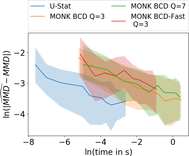
(a) Gaussian distribution, $N_{c}=0$ (no outlier), quadratic kernel.

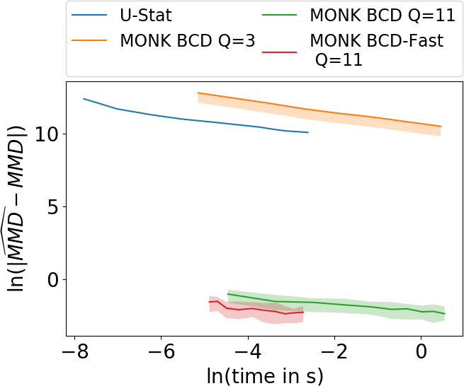
(b) Gaussian distribution, $N_{c}=5$ outliers, quadratic kernel.

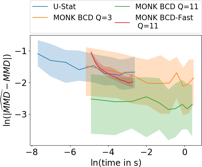
(c) Pareto distribution, quadratic kernel.

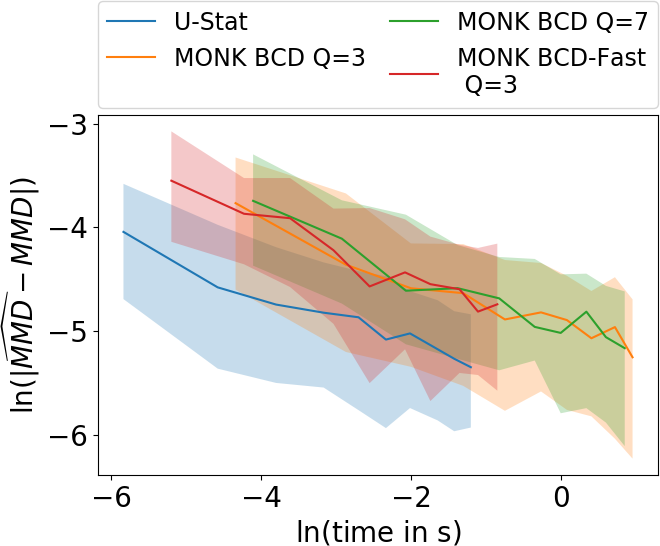
(d) Gaussian distribution, $N_{c}=0$ (no outlier), RBF kernel.

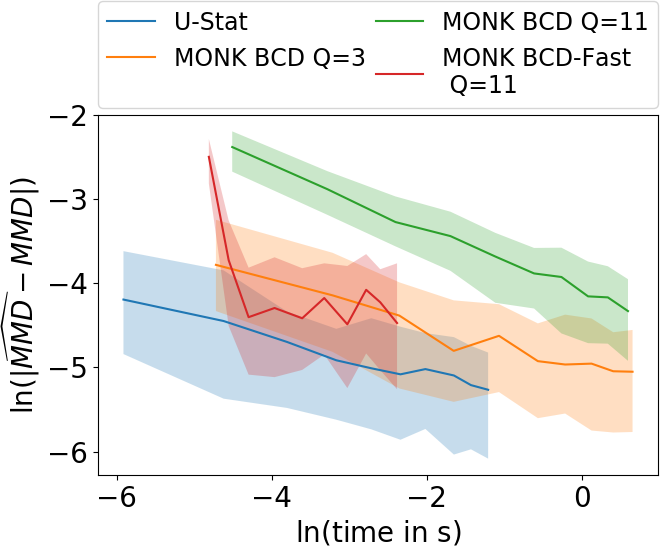
(e) Gaussian distribution, $N_{c}=5$ outliers, RBF kernel.

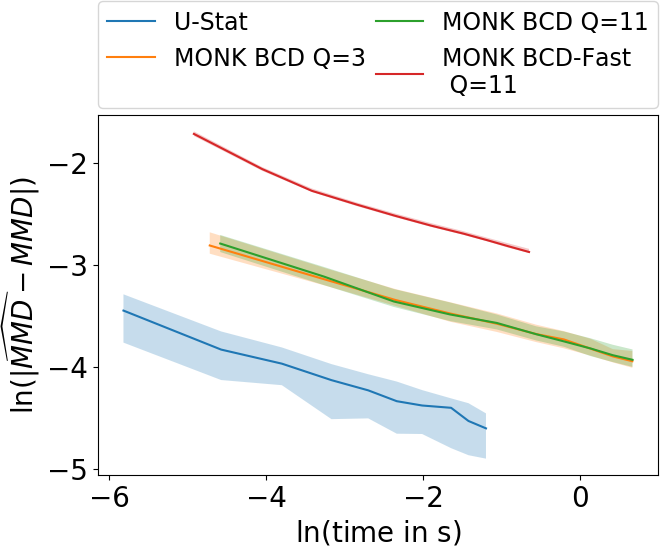
(f) Pareto distribution, RBF kernel.

Figure 1: Performance of the MMD estimators: median and quartiles of $\ln(|\widehat{\operatorname{MMD}}_{Q}(\mathbb{P},\mathbb{Q})-\operatorname{MMD}(\mathbb{P},\mathbb{Q})|)$. Columns from left to right: Experiment-1 – Experiment-3. Top: quadratic kernel, bottom: RBF kernel.

Experiment-2 (discrimination of DNA subsequences): In order to demonstrate the applicability of our estimators in biological context, we chose a DNA benchmark from the UCI repository (Dheeru & Karra Taniskidou, 2017), the Molecular Biology (Splice-junction Gene Sequences) Data Set. The dataset consists of $3190$ instances of $60$-character-long DNA subsequences. The problem is to recognize, given a sequence of DNA, the boundaries between exons (the parts of the DNA sequence retained after splicing) and introns (the parts of the DNA sequence that are spliced out). This task consists of two subproblems, identifying the exon/intron boundaries (referred to as EI sites) and the intron/exon boundaries (IE sites). We took $1532$ of these samples by selecting $766$ instances from both the EI and the IE classes (the class of those being neither EI nor IE is more heterogeneous and thus we dumped it from the study), and investigated the discriminability of the EI and IE categories. We represented the DNA sequences as strings ($\mathscr{X}$), chose $K$ as the String Subsequence Kernel (Lodhi et al., 2002) to compute MMD, and performed two-sample testing based on MMD using the MONK BCD, MONK BCD-Fast and U-Stat estimators. For completeness the pseudocode of the hypothesis test is detailed in Algorithm 3 (Section D). $Q$, the number of blocks in the MONK techniques, was equal to $5$. The significance level was $\alpha=0.05$. To assess the variability of the results $400$ Monte Carlo simulations were performed, each time uniformly sampling $N$ points without replacement resulting in $(X_{n})_{n\in[N]}$ and $(Y_{n})_{n\in[N]}$. To provide more detailed insights the aggregated values of $\widehat{\operatorname{MMD}}(\text{EI},\text{IE})-\hat{q}_{1-\alpha}$, $\widehat{\operatorname{MMD}}(\text{EI},\text{EI})-\hat{q}_{1-\alpha}$ and $\widehat{\operatorname{MMD}}(\text{IE},\text{IE})-\hat{q}_{1-\alpha}$ are summarized in Fig. 2, where $\hat{q}_{1-\alpha}$ is the estimated $(1-\alpha)$-quantile via $B=150$ bootstrap permutations. In the ideal case, $\widehat{\operatorname{MMD}}-\hat{q}_{1-\alpha}$ is positive (negative) in the inter-class (intra-class) experiments. As Fig. 2 shows all 3 techniques are able to solve the task, both in the inter-class (when the null hypothesis does not hold; Fig. 2a) and the intra-class experiment (null holds; Fig. 2b and Fig. 2c), and they converge to a good and stable performance as a function of the sample number. It is important to note that the MONK BCD-Fast method is especially well-adapted to problems where the kernel computation (such as the String Subsequence Kernel) or the sample size is a bottleneck, as its computation is often significantly faster compared to the U-Stat technique. For example, taking all the samples ($N=766$) in the DNA benchmark with $Q=15$, computing MONK BCD-Fast (U-Stat) takes $32s$ ($1m28s$). These results illustrate the applicability of our estimators in gene analysis.

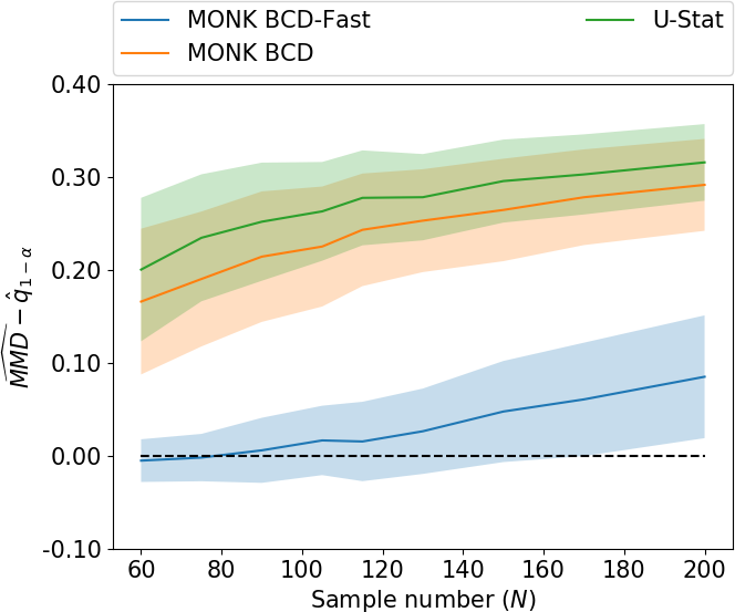
(a) Inter-class: EI-IE

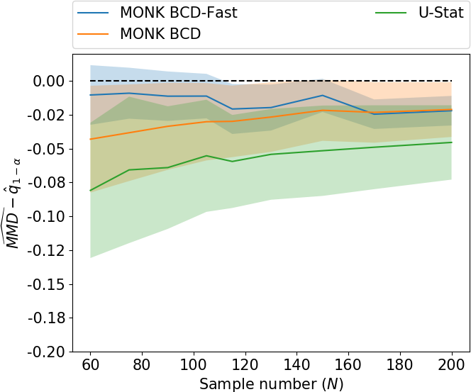
(b) Intra-class: EI-EI

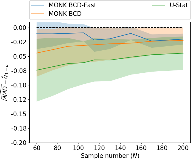
(c) Intra-class: IE-IE

Figure 2: Inter-class and intra-class MMD estimates as a function of the sample number compared to the bootstrap-estimated $(1-\alpha)$-quantile: $\widehat{\operatorname{MMD}}-\hat{q}_{1-\alpha}$; mean $\pm$ std. The null hypothesis is rejected iff $\widehat{\operatorname{MMD}}-\hat{q}_{1-\alpha}>0$. Notice the different scale of $\widehat{\operatorname{MMD}}-\hat{q}_{1-\alpha}$ in the inter-class and the intra-class experiments.

Supplement

The supplement contains the detailed proofs of our results (Section A), a few technical lemmas used during these arguments (Section B), the McDiarmid inequality for self-containedness (Section C), and the pseudocode of the two-sample test performed in Experiment-2 (Section D).

Appendix A Proofs of Theorem 1 and Theorem 2

This section contains the detailed proofs of Theorem 1 (Section A.1) and Theorem 2 (Section A.2).

A.1 Proof of Theorem 1

The structure of the proof is as follows:

1. We show that $\left\|\hat{\mu}_{\mathbb{P},Q}-\mu_{\mathbb{P}}\right\|_{K}\leq(1+\sqrt{2})r_{Q,N}$, where $r_{Q,N}=\sup_{f\in B_{K}}\text{MON}_{Q}\Big{[}\underbrace{\left\langle f,K(\cdot,x)-\mu_{\mathbb{P}}\right\rangle_{K}}_{f(x)-\mathbb{P}f}\Big{]}$, i.e. the analysis can be reduced to $B_{K}$.

2. Then $r_{Q,N}$ is bounded using empirical processes.

Step-1: Since $\mathscr{H}_{K}$ is an inner product space, for any $f\in\mathscr{H}_{K}$

$$\left\|f-K(\cdot,x)\right\|_{K}^{2}-\left\|\mu_{\mathbb{P}}-K(\cdot,x)\right\|_{K}^{2}$$

$$=\left\|f-\mu_{\mathbb{P}}\right\|_{K}^{2}-2\left\langle f-\mu_{\mathbb{P}},K(\cdot,x)-\mu_{\mathbb{P}}\right\rangle_{K}.$$ (14)

Hence, by denoting $e=\hat{\mu}_{\mathbb{P},Q}-\mu_{\mathbb{P}}$, $\tilde{g}=g-\mu_{\mathbb{P}}$ we get

$$\left\|e\right\|_{K}^{2}-2r_{Q,N}\left\|e\right\|_{K}$$

$$\stackrel{{\scriptstyle(a)}}{{\leq}}\left\|e\right\|_{K}^{2}-2\text{MON}_{Q}\left[\left\langle\frac{e}{\left\|e\right\|_{K}},K(\cdot,x)-\mu_{\mathbb{P}}\right\rangle\right]_{K}\left\|e\right\|_{K}$$

$$\stackrel{{\scriptstyle(b)}}{{\leq}}\text{MON}_{Q}\left[\left\|e\right\|_{K}^{2}-2\left\langle\frac{e}{\left\|e\right\|_{K}},K(\cdot,x)-\mu_{\mathbb{P}}\right\rangle_{K}\left\|e\right\|_{K}\right]$$

$$\stackrel{{\scriptstyle(c)}}{{\leq}}\text{MON}_{Q}\left[\left\|\hat{\mu}_{\mathbb{P},Q}-K(\cdot,x)\right\|_{K}^{2}-\left\|\mu_{\mathbb{P}}-K(\cdot,x)\right\|_{K}^{2}\right]$$

$$\stackrel{{\scriptstyle(d)}}{{\leq}}\sup_{g\in\mathscr{H}_{K}}\text{MON}_{Q}\left[\left\|\hat{\mu}_{\mathbb{P},Q}-K(\cdot,x)\right\|_{K}^{2}-\left\|g-K(\cdot,x)\right\|_{K}^{2}\right]$$

$$\stackrel{{\scriptstyle(e)}}{{\leq}}\sup_{g\in\mathscr{H}_{K}}\text{MON}_{Q}\left[\left\|\mu_{\mathbb{P}}-K(\cdot,x)\right\|_{K}^{2}-\left\|g-K(\cdot,x)\right\|_{K}^{2}\right]$$

$$\stackrel{{\scriptstyle(f)}}{{=}}\sup_{g\in\mathscr{H}_{K}}\Big{\{}2\text{MON}_{Q}\Big{[}{\underbrace{\left\langle\tilde{g},K(\cdot,x)-\mu_{\mathbb{P}}\right\rangle_{K}}_{\left\|\tilde{g}\right\|_{K}\left\langle\frac{\tilde{g}}{\left\|\tilde{g}\right\|_{K}},K(\cdot,x)-\mu_{\mathbb{P}}\right\rangle_{K}}}\Big{]}-\left\|\tilde{g}\right\|_{K}^{2}\Big{\}}$$

$$\stackrel{{\scriptstyle(g)}}{{=}}\sup_{g\in\mathscr{H}_{K}}\left\{2\left\|\tilde{g}\right\|_{K}r_{Q,N}-\left\|\tilde{g}\right\|_{K}^{2}\right\}\stackrel{{\scriptstyle(h)}}{{\leq}}r_{Q,N}^{2},$$ (15)

where we used in (a) the definition of $r_{Q,N}$, (b) the linearity of $\text{MON}_{Q}\left[\cdot\right]$, (c) Eq. (14), (d) $\sup_{g}$, (e) the definition of $\hat{\mu}_{\mathbb{P},Q}$, (f) Eq. (14) and the linearity of $\text{MON}_{Q}\left[\cdot\right]$, (g) the definition of $r_{Q,N}$. In step (h), by denoting $a=\left\|\tilde{g}\right\|_{K}$, $r=r_{Q,N}$, the argument of the $\sup$ takes the form $2ar-a^{2}$; $2ar-a^{2}\leq r^{2}\Leftrightarrow 0\leq r^{2}-2ar+a^{2}=(r-a)^{2}$.

In Eq. (15), we obtained an equation $a^{2}-2ra\leq r^{2}$ where $a:=\left\|e\right\|_{K}\geq 0$. Hence $r^{2}+2ra-a^{2}\geq 0$, $r_{1,2}=\left[-2a\pm\sqrt{4a^{2}+4a^{2}}\right]/2=\left(-1\pm\sqrt{2}\right)a$, thus by the non-negativity of $a$, $r\geq(-1+\sqrt{2})a$, i.e., $a\leq\frac{r}{\sqrt{2}-1}=(\sqrt{2}+1)r$. In other words, we arrived at

$$\left\|\hat{\mu}_{\mathbb{P},Q}-\mu_{\mathbb{P}}\right\|_{K} \leq\left(1+\sqrt{2}\right)r_{Q,N}.$$ (16)

It remains to upper bound $r_{Q,N}$.

Step-2: Our goal is to provide a probabilistic bound on

$$r_{Q,N}=\sup_{f\in B_{K}}\text{MON}_{Q}\left[x\mapsto\left\langle f,K(\cdot,x)-\mu_{\mathbb{P}}\right\rangle_{K}\right]$$

$$=\sup_{f\in B_{K}}\underset{q\in[Q]}{\text{med}}\{\underbrace{\left\langle f,\mu_{S_{q}}-\mu_{\mathbb{P}}\right\rangle_{K}}_{=:r(f,q)}\}.$$

The $N_{c}$ corrupted samples can affect (at most) $N_{c}$ of the $(S_{q})_{q\in[Q]}$ blocks. Let $U:=[Q]\backslash C$ stand for the indices of the uncorrupted sets, where $C:=\{q\in[Q]:\exists n_{j}\text{ s.t. }n_{j}\in S_{q},\,j\in[N_{c}]\}$ contains the indices of the corrupted sets. If

$$\forall f\in B_{K}:\underbrace{\left|\left\{q\in U:r(f,q)\geq\epsilon\right\}\right|}_{\sum_{q\in U}\mathbb{I}_{r(f,q)\geq\epsilon}}+N_{c}\leq\frac{Q}{2},$$ (17)

then for $\forall f\in B_{K}$, $\text{med}_{q\in[Q]}\{r(f,q)\}\leq\epsilon$, i.e. $\sup_{f\in B_{K}}\text{med}_{q\in[Q]}\{r(f,q)\}\leq\epsilon$. Thus, our task boils down to controlling the event in (17) by appropriately choosing $\epsilon$.

• Controlling $r(f,q)$: For any $f\in B_{K}$ the random variables $\left\langle f,k(\cdot,x_{i})-\mu_{\mathbb{P}}\right\rangle_{\mathscr{H}_{K}}=f(x_{i})-\mathbb{P}f$ are independent, have zero mean, and

  $$\mathbb{E}_{x_{i}\sim\mathbb{P}}\left\langle f,k(\cdot,x_{i})-\mu_{\mathbb{P}}\right\rangle_{K}^{2}=\left\langle f,\Sigma_{\mathbb{P}}f\right\rangle_{K}$$

  $$\leq\left\|f\right\|_{K}\left\|\Sigma_{\mathbb{P}}f\right\|_{K}\leq\left\|f\right\|_{K}^{2}\left\|\Sigma_{\mathbb{P}}\right\|=\left\|\Sigma_{\mathbb{P}}\right\|$$ (18)

  using the reproducing property of the kernel and the covariance operator, the Cauchy-Schwarz (CBS) inequality and $\left\|f\right\|_{\mathscr{H}_{K}}=1$.

  For a zero-mean random variable $z$ by the Chebyshev’s inequality $\mathbb{P}\left(z>a\right)\leq\mathbb{P}\left(|z|>a\right)\leq\mathbb{E}\left(z^{2}\right)/a^{2}$, which implies $\mathbb{P}\left(z>\sqrt{\mathbb{E}\left(z^{2}\right)/\alpha}\right)\leq\alpha$ by a $\alpha=\mathbb{E}\left(z^{2}\right)/a^{2}$ substitution. With $z:=r(f,q)$ ($q\in U$), using $\mathbb{E}\left[z^{2}\right]=\mathbb{E}\left\langle f,\mu_{S_{q}}-\mu_{\mathbb{P}}\right\rangle_{K}^{2}=\frac{Q}{N}\mathbb{E}_{x_{i}\sim\mathbb{P}}\left\langle f,k(\cdot,x_{i})-\mu_{\mathbb{P}}\right\rangle_{K}^{2}$ and Eq. (18) one gets that for all $f\in B_{K}$, $\alpha\in(0,1)$ and $q\in U$: $\mathbb{P}\left(r(f,q)>\sqrt{\frac{\left\|\Sigma_{\mathbb{P}}\right\|Q}{\alpha N}}\right)\leq\alpha$. This means $\mathbb{P}\left(r(f,q)>\frac{\epsilon}{2}\right)\leq\alpha$ with $\epsilon\geq 2\sqrt{\frac{\left\|\Sigma_{\mathbb{P}}\right\|Q}{\alpha N}}$.

• Reduction to $\phi$: As a result

  $$\sum_{q\in U}\mathbb{P}\left(r(f,q)\geq\frac{\epsilon}{2}\right)\leq|U|\alpha$$

  happens if and only if

  $$\sum_{q\in U}\mathbb{I}_{r(f,q)\geq\epsilon}$$

  $$\leq|U|\alpha+\sum_{q\in U}\Big{[}\mathbb{I}_{r(f,q)\geq\epsilon}-\underbrace{\mathbb{P}\left(r(f,q)\geq\frac{\epsilon}{2}\right)}_{\mathbb{E}\left[\mathbb{I}_{r(f,q)\geq\frac{\epsilon}{2}}\right]}\Big{]}=:A.$$

  Let us introduce $\phi:t\in\mathbb{R}\to(t-1)\mathbb{I}_{1\leq t\leq 2}+\mathbb{I}_{t\geq 2}$. $\phi$ is $1$-Lipschitz and satisfies $\mathbb{I}_{2\leq t}\leq\phi(t)\leq\mathbb{I}_{1\leq t}$ for any $t\in\mathbb{R}$. Hence, we can upper bound $A$ as

  $$A \leq|U|\alpha+\sum_{q\in U}\left[\phi\left(\frac{2r(f,q)}{\epsilon}\right)-\mathbb{E}\phi\left(\frac{2r(f,q)}{\epsilon}\right)\right]$$

  by noticing that $\epsilon\leq r(f,q)\Leftrightarrow 2\leq 2r(f,q)/\epsilon$ and $\epsilon/2\leq r(f,q)\Leftrightarrow 1\leq 2r(f,q)/\epsilon$, and by using the $\mathbb{I}_{2\leq t}\leq\phi(t)$ and the $\phi(t)\leq\mathbb{I}_{1\leq t}$ bound, respectively. Taking supremum over $B_{K}$ we arrive at

  $$\sup_{f\in B_{K}}\sum_{q\in U}\mathbb{I}_{r(f,q)\geq\epsilon}$$

  $$\leq|U|\alpha+\underbrace{\sup_{f\in B_{K}}\sum_{q\in U}\left[\phi\left(\frac{2r(f,q)}{\epsilon}\right)-\mathbb{E}\phi\left(\frac{2r(f,q)}{\epsilon}\right)\right]}_{=:Z}.$$

• Concentration of $Z$ around its mean: Notice that $Z$ is a function of $x_{V}$, the samples in the uncorrupted blocks; $V=\cup_{q\in U}S_{q}$. By the bounded difference property of $Z$ (Lemma 4) for any $\beta>0$, the McDiarmid inequality (Lemma 6; we choose $\tau:=Q\beta^{2}/8$ to get linear scaling in $Q$ on the r.h.s.) implies that

  $$\mathbb{P}\left(Z<\mathbb{E}_{x_{V}}[Z]+Q\beta\right)\geq 1-e^{-\frac{Q\beta^{2}}{8}}.$$

• Bounding $\mathbb{E}_{x_{V}}[Z]$: Let $M=N/Q$ denote the number of elements in $S_{q}$-s. The $\mathscr{G}=\{g_{f}:f\in B_{K}\}$ class with $g_{f}:\mathscr{X}^{M}\rightarrow\mathbb{R}$ and $\mathbb{P}_{M}:=\frac{1}{M}\sum_{m=1}^{M}\delta_{u_{m}}$ defined as

  $$g_{f}(u_{1:M}) =\phi\left(\frac{\left\langle f,\mu_{\mathbb{P}_{M}}-\mu_{\mathbb{P}}\right\rangle_{K}}{\epsilon}\right)$$

  is uniformly bounded separable Carathéodory (Lemma 5), hence the symmetrization technique (Steinwart & Christmann, 2008, Prop. 7.10), (Ledoux & Talagrand, 1991) gives

  $$\mathbb{E}_{x_{V}}[Z]\leq 2\mathbb{E}_{x_{V}}\mathbb{E}_{\mathbf{e}}\sup_{f\in B_{K}}\left|\sum_{q\in U}e_{q}\phi\left(\frac{2r(f,q)}{\epsilon}\right)\right|,$$

  where $\mathbf{e}=(e_{q})_{q\in U}\in\mathbb{R}^{|U|}$ with i.i.d. Rademacher entries [$\mathbb{P}(e_{q}=\pm 1)=\frac{1}{2}$ ($\forall q$)].

• Discarding $\phi$: Since $\phi(0)=0$ and $\phi$ is 1-Lipschitz, by Talagrand’s contraction principle of Rademacher processes (Ledoux & Talagrand, 1991), (Koltchinskii, 2011, Theorem 2.3) one gets

  $$\mathbb{E}_{x_{V}}\mathbb{E}_{\mathbf{e}}\sup_{f\in B_{K}}\left|\sum_{q\in U}e_{q}\phi\left(\frac{2r(f,q)}{\epsilon}\right)\right|$$

  $$\leq 2\mathbb{E}_{x_{V}}\mathbb{E}_{\mathbf{e}}\sup_{f\in B_{K}}\left|\sum_{q\in U}e_{q}\frac{2r(f,q)}{\epsilon}\right|.$$

• Switching from $|U|$ to $N$ terms: Applying an other symmetrization [(a)], the CBS inequality, $f\in B_{K}$, and the Jensen inequality

  $$\mathbb{E}_{x_{V}}\mathbb{E}_{\mathbf{e}}\sup_{f\in B_{K}}\left|\sum_{q=1}^{Q}e_{q}\frac{r(f,q)}{\epsilon}\right|$$

  $$\stackrel{{\scriptstyle(a)}}{{\leq}}\frac{2Q}{\epsilon N}\mathbb{E}_{x_{V}}\mathbb{E}_{\mathbf{e}^{\prime}}\Bigg{[}\sup_{f\in B_{K}}\Big{|}\underbrace{\sum_{n\in V}e_{n}^{\prime}\left<f,K(\cdot,x_{n})-\mu_{\mathbb{P}}\right>_{K}}_{=\left<f,\sum_{n\in V}e_{n}^{\prime}\left[K(\cdot,x_{n})-\mu_{\mathbb{P}}\right]\right>_{K}}\Big{|}\Bigg{]}$$

  $$\leq\frac{2Q}{\epsilon N}\mathbb{E}_{x_{V}}\mathbb{E}_{\mathbf{e}^{\prime}}\left[\sup_{f\in B_{K}}\underbrace{\left\|f\right\|_{K}}_{=1}\left\|\sum_{n\in V}e_{n}^{\prime}\left[K(\cdot,x_{n})-\mu_{\mathbb{P}}\right]\right\|_{K}\right]$$

  $$=\frac{2Q}{\epsilon N}\mathbb{E}_{x_{V}}\mathbb{E}_{\mathbf{e}^{\prime}}\left\|\sum_{n\in V}e_{n}^{\prime}\left[K(\cdot,x_{n})-\mu_{\mathbb{P}}\right]\right\|_{K}$$

  $$\leq\frac{2Q}{\epsilon N}\sqrt{\mathbb{E}_{x_{V}}\mathbb{E}_{\mathbf{e}^{\prime}}\left\|\sum_{n\in V}e_{n}^{\prime}\left[K(\cdot,x_{n})-\mu_{\mathbb{P}}\right]\right\|_{K}^{2}}$$

  $$\stackrel{{\scriptstyle(b)}}{{=}}\frac{2Q\sqrt{|V|\operatorname{\operatorname{Tr}}(\Sigma_{\mathbb{P}})}}{\epsilon N}.$$

  In (a), we proceed as follows:

  $$\mathbb{E}_{x_{V}}\mathbb{E}_{\mathbf{e}}\sup_{f\in B_{K}}\left|\sum_{q\in U}e_{q}\frac{r(f,q)}{\epsilon}\right|$$

  $$=\mathbb{E}_{x_{V}}\mathbb{E}_{\mathbf{e}}\sup_{f\in B_{K}}\left|\sum_{q\in U}e_{q}\frac{\left<f,\mu_{S_{q}}-\mu_{\mathbb{P}}\right>_{K}}{\epsilon}\right|$$

  $$\stackrel{{\scriptstyle(c)}}{{\leq}}\frac{2Q}{N\epsilon}\mathbb{E}_{x_{V}}\mathbb{E}_{\mathbf{e}}\mathbb{E}_{\mathbf{e}^{\prime}}\sup_{f\in B_{K}}\left|\sum_{n\in V}e_{n}^{\prime}e_{n}^{\prime\prime}\left<f,K(\cdot,x_{n})-\mu_{\mathbb{P}}\right>_{K}\right|$$

  $$=\frac{2Q}{N\epsilon}\mathbb{E}_{x_{V}}\mathbb{E}_{\mathbf{e}^{\prime}}\sup_{f\in B_{K}}\left|\sum_{n\in V}e_{n}^{\prime}\left<f,K(\cdot,x_{n})-\mu_{\mathbb{P}}\right>_{K}\right|,$$

  where in (c) we applied symmetrization, $\mathbf{e}^{\prime}=(e_{n}^{\prime})_{n\in V}\in\mathbb{R}^{|V|}$ with i.i.d. Rademacher entries, $e_{n}^{\prime\prime}=e_{q}$ if $n\in S_{q}$ ($q\in U$), and we used that $\left(e_{n}^{\prime}e_{n}^{\prime\prime}\left<f,K(\cdot,x_{n})-\mu_{\mathbb{P}}\right>_{K}\right)_{n\in V}\stackrel{{\scriptstyle\text{distr}}}{{=}}\left(e_{n}^{\prime}\left<f,K(\cdot,x_{n})-\mu_{\mathbb{P}}\right>_{K}\right)_{n\in V}$.

  In step (b), we had

  $$\mathbb{E}_{x_{V}}\mathbb{E}_{\mathbf{e}^{\prime}}\left\|\sum\nolimits_{n\in V}e_{n}^{\prime}\left[K(\cdot,x_{n})-\mu_{\mathbb{P}}\right]\right\|_{K}^{2}$$

  $$=\mathbb{E}_{x_{V}}\mathbb{E}_{\mathbf{e}^{\prime}}\sum_{n\in V}\left[e_{n}^{\prime}\right]^{2}\left<K(\cdot,x_{n})-\mu_{\mathbb{P}},K(\cdot,x_{n})-\mu_{\mathbb{P}}\right>_{K}$$

  $$=|V|\mathbb{E}_{x\sim\mathbb{P}}\left<K(\cdot,x)-\mu_{\mathbb{P}},K(\cdot,x)-\mu_{\mathbb{P}}\right>_{K}$$

  $$=|V|\mathbb{E}_{x\sim\mathbb{P}}\operatorname{\operatorname{Tr}}\left([K(\cdot,x)-\mu_{\mathbb{P}}]\otimes[K(\cdot,x)-\mu_{\mathbb{P}}]\right)$$

  $$=|V|\operatorname{\operatorname{Tr}}(\Sigma_{\mathbb{P}})$$

  exploiting the independence of $e_{n}^{\prime}$-s and $[e_{n}^{\prime}]^{2}=1$.

Until this point we showed that for all $\alpha\in(0,1)$, $\beta>0$, if $\epsilon\geq 2\sqrt{\frac{\left\|\Sigma_{\mathbb{P}}\right\|Q}{\alpha N}}$ then

$$\sup_{f\in B_{K}}\sum_{q=1}^{Q}\mathbb{I}_{r(f,q)\geq\epsilon}\leq|U|\alpha+Q\beta+\frac{8Q\sqrt{|V|\operatorname{\operatorname{Tr}}(\Sigma_{\mathbb{P}})}}{\epsilon N}$$

with probability at least $1-e^{-\frac{Q\beta^{2}}{8}}$. Thus, to ensure that $\sup_{f\in B_{K}}\sum_{q=1}^{Q}\mathbb{I}_{r(f,q)\geq\epsilon}+N_{c}\leq Q/2$ it is sufficient to choose $(\alpha,\beta,\epsilon)$ such that $|U|\alpha+Q\beta+\frac{8Q\sqrt{|V|\operatorname{\operatorname{Tr}}(\Sigma_{\mathbb{P}})}}{\epsilon N}+N_{c}\leq\frac{Q}{2}$, and in this case $\left\|\hat{\mu}_{\mathbb{P},Q}-\mu_{\mathbb{P}}\right\|_{K}\leq(1+\sqrt{2})\epsilon$. Applying the $|U|\leq Q$ and $|V|\leq N$ bounds, we want to have

$$Q\alpha+Q\beta+\frac{8Q\sqrt{\operatorname{\operatorname{Tr}}(\Sigma_{\mathbb{P}})}}{\epsilon\sqrt{N}}+N_{c}\leq\frac{Q}{2}.$$ (19)

Choosing $\alpha=\beta=\frac{\delta}{3}$ in Eq. (19), the sum of the first two terms is $Q\frac{2\delta}{3}$; $\epsilon\geq\max\left(2\sqrt{\frac{3\left\|\Sigma_{\mathbb{P}}\right\|Q}{\delta N}},\frac{24}{\delta}\sqrt{\frac{\operatorname{\operatorname{Tr}}{\left(\Sigma_{\mathbb{P}}\right)}}{N}}\right)$ gives $\leq Q\frac{\delta}{3}$ for the third term. Since $N_{c}\leq Q(\frac{1}{2}-\delta)$, we got

$$\left\|\hat{\mu}_{\mathbb{P},Q}-\mu_{\mathbb{P}}\right\|_{K}\leq c_{1}\max\left(\sqrt{\frac{3\left\|\Sigma_{\mathbb{P}}\right\|Q}{\delta N}},\frac{12}{\delta}\sqrt{\frac{\operatorname{\operatorname{Tr}}{(\Sigma_{\mathbb{P}})}}{N}}\right)$$

with probability at least $1-\mathrm{e}^{-\frac{Q\delta^{2}}{72}}$. With an $\eta=\mathrm{e}^{-\frac{Q\delta^{2}}{72}}$, and hence $Q=\frac{72\ln\left(\frac{1}{\eta}\right)}{\delta^{2}}$ reparameterization Theorem 1 follows.

A.2 Proof of Theorem 2

The reasoning is similar to Theorem 1; we detail the differences below. The high-level structure of the proof is as follows:

• First we prove that $\big{|}\widehat{\operatorname{MMD}}_{Q}(\mathbb{P},\mathbb{Q})-\operatorname{MMD}(\mathbb{P},\mathbb{Q})\big{|}\leq r_{Q,N}$, where $r_{Q,N}=\sup\limits_{f\in B_{K}}\Big{|}\underset{q\in[Q]}{\text{med}}\left\{\left<f,\left(\mu_{S_{q},\mathbb{P}}-\mu_{S_{q},\mathbb{Q}}\right)-(\mu_{\mathbb{P}}-\mu_{\mathbb{Q}})\right>_{K}\right\}\Big{|}$.

• Then $r_{Q,N}$ is bounded.

Step-1:

• $\widehat{\operatorname{MMD}}_{Q}(\mathbb{P},\mathbb{Q})-\operatorname{MMD}(\mathbb{P},\mathbb{Q})\leq r_{Q,N}$: By the subadditivity of supremum [$\sup_{f}(a_{f}+b_{f})\leq\sup_{f}a_{f}+\sup_{f}b_{f}$] one gets

  $$\widehat{\operatorname{MMD}}_{Q}(\mathbb{P},\mathbb{Q})$$

  $$=\sup_{f\in B_{K}}\underset{q\in[Q]}{\text{med}}\big{\{}\big{<}f,\left(\mu_{S_{q},\mathbb{P}}-\mu_{S_{q},\mathbb{Q}}\right)-(\mu_{\mathbb{P}}-\mu_{\mathbb{Q}})$$

  $$\hskip 28.45274pt+(\mu_{\mathbb{P}}-\mu_{\mathbb{Q}})\big{>}_{K}\big{\}}$$

  $$\leq\sup_{f\in B_{K}}\underset{q\in[Q]}{\text{med}}\left\{\left<f,\left(\mu_{S_{q},\mathbb{P}}-\mu_{S_{q},\mathbb{Q}}\right)-(\mu_{\mathbb{P}}-\mu_{\mathbb{Q}})\right>_{K}\right\}$$

  $$\hskip 28.45274pt+\sup_{f\in B_{K}}\left<f,\mu_{\mathbb{P}}-\mu_{\mathbb{Q}}\right>_{K}$$

  $$\leq\underbrace{\sup_{f\in B_{K}}\left|\underset{q\in[Q]}{\text{med}}\left\{\left<f,\left(\mu_{S_{q},\mathbb{P}}-\mu_{S_{q},\mathbb{Q}}\right)-(\mu_{\mathbb{P}}-\mu_{\mathbb{Q}})\right>_{K}\right\}\right|}_{=r_{Q,N}}$$

  $$\hskip 28.45274pt+\operatorname{MMD}(\mathbb{P},\mathbb{Q}).$$

• $\operatorname{MMD}_{Q}(\mathbb{P},\mathbb{Q})-\widehat{\operatorname{MMD}}_{Q}(\mathbb{P},\mathbb{Q})\leq r_{Q,N}$: Let $a_{f}:=\left<f,\mu_{\mathbb{P}}-\mu_{\mathbb{Q}}\right>_{K}$ and $b_{f}:=\underset{q\in[Q]}{\text{med}}\left\{\left<f,(\mu_{\mathbb{P}}-\mu_{\mathbb{Q}})-(\mu_{S_{q},\mathbb{P}}-\mu_{S_{q},\mathbb{Q}})\right>_{K}\right\}$. Then

  $$a_{f}-b_{f}$$

  $$=\left<f,\mu_{\mathbb{P}}-\mu_{\mathbb{Q}}\right>_{K}$$

  $$\hskip 14.22636pt+\text{med}_{q\in[Q]}\left\{\left<f,(\mu_{S_{q},\mathbb{P}}-\mu_{S_{q},\mathbb{Q}})-(\mu_{\mathbb{P}}-\mu_{\mathbb{Q}})\right>_{K}\right\}$$

  $$=\text{med}_{q\in[Q]}\left\{\left<f,\mu_{S_{q},\mathbb{P}}-\mu_{S_{q},\mathbb{Q}}\right>_{K}\right\}$$

  by $\text{med}_{q\in[Q]}\{-z_{q}\}=-\text{med}_{q\in[Q]}\{z_{q}\}$. Applying the $\sup_{f}(a_{f}-b_{f})\geq\sup_{f}a_{f}-\sup_{f}b_{f}$ inequality (it follows from the subadditivity of $\sup$):

  $$\widehat{\operatorname{MMD}}_{Q}(\mathbb{P},\mathbb{Q})$$

  $$\geq\operatorname{MMD}(\mathbb{P},\mathbb{Q})$$

  $$\hskip 14.22636pt-\sup_{f\in B_{K}}\underbrace{\underset{q\in[Q]}{\text{med}}\big{\{}\big{<}f,(\mu_{\mathbb{P}}-\mu_{\mathbb{Q}})-(\mu_{S_{q},\mathbb{P}}-\mu_{S_{q},\mathbb{Q}})\big{>}_{K}\big{\}}}_{-\underset{q\in[Q]}{\text{med}}\left\{\left<f,(\mu_{S_{q},\mathbb{P}}-\mu_{S_{q},\mathbb{Q}})-(\mu_{\mathbb{P}}-\mu_{\mathbb{Q}})\right>_{K}\right\}}$$

  $$\geq\operatorname{MMD}(\mathbb{P},\mathbb{Q})$$

  $$\hskip 14.22636pt-\underbrace{\sup_{f\in B_{K}}\left|\underset{q\in[Q]}{\text{med}}\left\{\left<f,(\mu_{S_{q},\mathbb{P}}-\mu_{S_{q},\mathbb{Q}})-(\mu_{\mathbb{P}}-\mu_{\mathbb{Q}})\right>_{K}\right\}\right|}_{r_{Q,N}}.$$

Step-2: Our goal is to control

$$r_{Q,N} =\sup\nolimits_{f\in B_{K}}\Big{|}\text{med}_{q\in[Q]}\Big{\{}r(f,q)\Big{\}}\Big{|},\text{ where}$$

$$r(f,q) :=\left<f,(\mu_{S_{q},\mathbb{P}}-\mu_{S_{q},\mathbb{Q}})-(\mu_{\mathbb{P}}-\mu_{\mathbb{Q}})\right>_{K}.$$

The relevant quantities which change compared to the proof of Theorem 1 are as follows.

• Median rephrasing:

  $$\sup_{f\in B_{K}}\Big{|}\underset{q\in[Q]}{\text{med}}\{r(f,q)\}\Big{|}\leq\epsilon$$

  $$\Leftrightarrow\forall f\in B_{K}:-\epsilon\leq\text{med}_{q\in[Q]}\{r(f,q)\}\leq\epsilon$$

  $$\Leftarrow\forall f\in B_{K}:\left|\left\{q:r(f,q)\leq-\epsilon\right\}\right|\leq Q/2$$

  $$\hskip 14.22636pt\text{ and }\left|\left\{q:r(f,q)\geq\epsilon\right\}\right|\leq Q/2$$

  $$\Leftarrow\forall f\in B_{K}:\left|\left\{q:|r(f,q)|\geq\epsilon\right\}\right|\leq Q/2.$$

  Thus, $\forall f\in B_{K}:\left|\left\{q\in U:|r(f,q)|\geq\epsilon\right\}\right|+N_{c}\leq\frac{Q}{2}$, implies $\sup_{f\in B_{K}}\Big{|}\text{med}_{q\in[Q]}\{r(f,q)\}\Big{|}\leq\epsilon$.

• Controlling $|r(f,q)|$: For any $f\in B_{K}$ the random variables $[f(x_{i})-f(y_{i})]-[\mathbb{P}f-\mathbb{Q}f]$ are independent, zero-mean and

  $$\mathbb{E}_{(x,y)\sim\mathbb{P}\otimes\mathbb{Q}}([f(x)-\mathbb{P}f]-[f(y)-\mathbb{Q}f])^{2}$$

  $$=\mathbb{E}_{x\sim\mathbb{P}}[f(x)-\mathbb{P}f]^{2}+\mathbb{E}_{y\sim\mathbb{Q}}[f(y)-\mathbb{Q}f]^{2}$$

  $$\leq\left\|\Sigma_{\mathbb{P}}\right\|+\left\|\Sigma_{\mathbb{Q}}\right\|,$$

  where $\mathbb{P}\otimes\mathbb{Q}$ is the product measure. The Chebyshev argument with $z=|r(f,q)|$ implies that $\forall\alpha\in(0,1)$

  $$(\mathbb{P}\otimes\mathbb{Q})\left(|r(f,q)|>\sqrt{\frac{\left(\left\|\Sigma_{\mathbb{P}}\right\|+\left\|\Sigma_{\mathbb{Q}}\right\|\right)Q}{\alpha N}}\right)\leq\alpha.$$

  This means $(\mathbb{P}\otimes\mathbb{Q})\left(|r(f,q)|>\epsilon/2\right)\leq\alpha$ with $\epsilon\geq 2\sqrt{\frac{\left(\left\|\Sigma_{\mathbb{P}}\right\|+\left\|\Sigma_{\mathbb{Q}}\right\|\right)Q}{\alpha N}}$.

• Switching from $|U|$ to $N$ terms: With $(xy)_{V}=\left\{(x_{i},y_{i}):i\in V\right\}$, in ’(b)’ with $\tilde{x}_{n}:=K(\cdot,x_{n})-\mu_{\mathbb{P}}$, $\tilde{y}_{n}:=K(\cdot,y_{n})-\mu_{\mathbb{Q}}$ we arrive at

  $$\mathbb{E}_{(xy)_{V}}\mathbb{E}_{\mathbf{e}^{\prime}}\left\|\sum_{n\in V}e_{n}^{\prime}\left(\tilde{x}_{n}-\tilde{y}_{n}\right)\right\|_{K}^{2}$$

  $$=\mathbb{E}_{(xy)_{V}}\mathbb{E}_{\mathbf{e}^{\prime}}\sum_{n\in V}\left[e_{n}^{\prime}\right]^{2}\left<\tilde{x}_{n}-\tilde{y}_{n},\tilde{x}_{n}-\tilde{y}_{n}\right>_{K}$$

  $$=|V|\mathbb{E}_{(xy)\sim\mathbb{P}}\left\|\left[K(\cdot,x)-\mu_{\mathbb{P}}\right]-\left[K(\cdot,y)-\mu_{\mathbb{Q}}\right]\right\|_{K}$$

  $$=|V|\left[\operatorname{\operatorname{Tr}}\left(\Sigma_{\mathbb{P}}\right)+\operatorname{\operatorname{Tr}}\left(\Sigma_{\mathbb{Q}}\right)\right].$$

• These results imply

  $$Q\alpha+Q\beta+\frac{8Q\sqrt{\operatorname{\operatorname{Tr}}\left(\Sigma_{\mathbb{P}}\right)+\operatorname{\operatorname{Tr}}\left(\Sigma_{\mathbb{Q}}\right)}}{\epsilon\sqrt{N}}+N_{c}\leq Q/2.$$

  $\epsilon\geq\max\left(2\sqrt{\frac{3\left(\left\|\Sigma_{\mathbb{P}}\right\|+\left\|\Sigma_{\mathbb{Q}}\right\|\right)Q}{\delta N}},\frac{24}{\delta}\sqrt{\frac{\operatorname{\operatorname{Tr}}{\left(\Sigma_{\mathbb{P}}\right)}+\operatorname{\operatorname{Tr}}{\left(\Sigma_{\mathbb{Q}}\right)}}{N}}\right)$, $\alpha=\beta=\frac{\delta}{3}$ choice gives that

  $$\left|\widehat{\operatorname{MMD}}_{Q}(\mathbb{P},\mathbb{Q})-\operatorname{MMD}(\mathbb{P},\mathbb{Q})\right|$$

  $$\leq 2\max\left(\sqrt{\frac{3\left(\left\|\Sigma_{\mathbb{P}}\right\|+\left\|\Sigma_{\mathbb{Q}}\right\|\right)Q}{\delta N}},\frac{12}{\delta}\sqrt{\frac{\operatorname{\operatorname{Tr}}{(\Sigma_{\mathbb{P}})}+\operatorname{\operatorname{Tr}}{(\Sigma_{\mathbb{Q}})}}{N}}\right)$$

  with probability at least $1-e^{-\frac{Q\delta^{2}}{72}}$. $\eta=e^{-\frac{Q\delta^{2}}{72}}$, i.e. $Q=\frac{72\ln\left(\frac{1}{\eta}\right)}{\delta^{2}}$ reparameterization finishes the proof of Theorem 2.

Appendix B Technical Lemmas

Lemma 3 (Supremum).

$$\Big{|}\sup_{f}a_{f}-\sup_{f}b_{f}\Big{|}\leq\sup_{f}|a_{f}-b_{f}|.$$

Lemma 4 (Bounded difference property of $Z$).

Let $N\in\mathbb{Z}^{+}$, $(S_{q})_{q\in[Q]}$ be a partition of $[N]$, $K:\mathscr{X}\times\mathscr{X}\rightarrow\mathbb{R}$ be a kernel, $\mu$ be the mean embedding associated to $K$, $x_{1:N}$ be i.i.d. random variables on $\mathscr{X}$, $Z(x_{V})=\sup\limits_{f\in B_{K}}\sum\limits_{q\in U}\left[\phi\left(\frac{2\left<f,\mu_{S_{q}}-\mu_{\mathbb{P}}\right>_{K}}{\epsilon}\right)-\mathbb{E}\phi\left(\frac{2\left<f,\mu_{S_{q}}-\mu_{\mathbb{P}}\right>_{K}}{\epsilon}\right)\right]$, where $U\subseteq[Q]$, $V=\cup_{q\in U}S_{q}$. Let $x_{V_{i}}^{\prime}$ be $x_{V}$ except for the $i\in V$-th coordinate; $x_{i}$ is changed to $x_{i}^{\prime}$. Then

$$\sup_{x_{V}\in\mathscr{X}^{|V|},x_{i}^{\prime}\in\mathscr{X}}\left|Z\left(x_{V}\right)-Z\left(x_{V_{i}}^{\prime}\right)\right|\leq 4,\,\forall i\in V.$$

Proof.

Since $(S_{q})_{q\in[Q]}$ is a partition of $[Q]$, $(S_{q})_{q\in U}$ forms a partition of $V$ and there exists a unique $r\in U$ such that $i\in S_{r}$. Let

$$Y_{q}:=Y_{q}(f,x_{V}),$$

$$q\in U=\phi\left(\frac{2\left<f,\mu_{S_{q}}-\mu_{\mathbb{P}}\right>_{K}}{\epsilon}\right)-\mathbb{E}\phi\left(\frac{2\left<f,\mu_{S_{q}}-\mu_{\mathbb{P}}\right>_{K}}{\epsilon}\right),$$

$$Y_{r}^{\prime}:=Y_{r}(f,x_{V_{i}}^{\prime}).$$

In this case

$$\left|Z\left(x_{V}\right)-Z\left(x_{V_{i}}^{\prime}\right)\right|$$

$$=\left|\sup_{f\in B_{K}}\sum_{q\in U}Y_{q}-\sup_{f\in B_{K}}\left(\sum_{q\in U\backslash\{r\}}Y_{q}+Y_{r}^{\prime}\right)\right|$$

$$\stackrel{{\scriptstyle(a)}}{{\leq}}\sup_{f\in B_{K}}\left|Y_{r}-Y_{r}^{\prime}\right|\stackrel{{\scriptstyle(b)}}{{\leq}}\sup_{f\in B_{K}}\Big{(}\underbrace{\left|Y_{r}\right|}_{\leq 2}+\underbrace{\left|Y_{r}^{\prime}\right|}_{\leq 2}\Big{)}\leq 4,$$

where in (a) we used Lemma 3, (b) the triangle inequality and the boundedness of $\phi$ [$|\phi(t)|\leq 1$ for all $t$].

∎

Lemma 5 (Uniformly bounded separable Carathéodory family).

Let $\epsilon>0$, $N\in\mathbb{Z}^{+}$, $Q\in\mathbb{Z}^{+}$, $M=N/Q\in\mathbb{Z}^{+}$, $\phi(t)=(t-1)\mathbb{I}_{1\leq t\leq 2}+\mathbb{I}_{t\geq 2}$, $K:\mathscr{X}\times\mathscr{X}\rightarrow\mathbb{R}$ is a continuous kernel on the separable topological domain $\mathscr{X}$, $\mu$ is the mean embedding associated to $K$, $\mathbb{P}_{M}:=\frac{1}{M}\sum_{m=1}^{M}\delta_{u_{m}}$, $\mathscr{G}=\{g_{f}:f\in B_{K}\}$, where $g_{f}:\mathscr{X}^{M}\rightarrow\mathbb{R}$ is defined as

$$g_{f}(u_{1:M}) =\phi\left(\frac{2\left<f,\mu_{\mathbb{P}_{M}}-\mu_{\mathbb{P}}\right>_{K}}{\epsilon}\right).$$

Then $\mathscr{G}$ is a uniformly bounded separable Carathéodory family: (i) $\sup_{f\in B_{K}}\left\|g_{f}\right\|_{\infty}<\infty$ where $\left\|g\right\|_{\infty}=\sup_{u_{1:M}\in\mathscr{X}^{M}}|g(u_{1:M})|$, (ii) $u_{1:M}\mapsto g_{f}(u_{1:M})$ is measurable for all $f\in B_{K}$, (iii) $f\mapsto g_{f}(u_{1:M})$ is continuous for all $u_{1:M}\in\mathscr{X}^{M}$, (iv) $B_{K}$ is separable.

Proof.

• $|\phi(t)|\leq 1$ for any $t$, hence $\left\|g_{f}\right\|_{\infty}\leq 1$ for all $f\in B_{K}$.

• Any $f\in B_{K}$ is continuous since $\mathscr{H}_{K}\subset C(\mathscr{X})=\{h:\mathscr{X}\rightarrow\mathbb{R}\text{ continuous}\}$, so $u_{1:M}\mapsto(f(u_{1}),\ldots,f(u_{M}))$ is continuous. $\phi$ is Lipschitz, specifically continuous. The continuity of these two maps imply that of $u_{1:M}\mapsto g_{f}(u_{1:M})$, specifically it is Borel-measurable.

• The statement follows by the continuity of $f\mapsto\left<f,h\right>_{K}$ ($h=\mu_{\mathbb{P}_{M}}-\mu_{\mathbb{P}}$) and that of $\phi$.

• $B_{K}$ is separable since $\mathscr{H}_{K}$ is so by assumption.

∎

Appendix C External Lemma

Below we state the McDiarmid inequality for self-containedness.

Lemma 6 (McDiarmid inequality).

Let $x_{1:N}$ be $\mathscr{X}$-valued independent random variables. Assume that $f:\mathscr{X}^{N}\rightarrow\mathbb{R}$ satisfies the bounded difference property

$$\sup_{u_{1},\ldots,u_{N},u_{r}^{\prime}\in\mathscr{X}}\left|f(u_{1:N})-f(u_{1:N}^{\prime})\right|\leq c,\quad\forall n\in[N],$$

where $u_{1:N}^{\prime}=\left(u_{1},\ldots,u_{n-1},u_{n}^{\prime},u_{n+1},\ldots,u_{N}\right)$. Then for any $\tau>0$

$$\mathbb{P}\left(f(x_{1:N})<\mathbb{E}_{x_{1:N}}\left[f(x_{1:N})\right]+c\sqrt{\frac{\tau N}{2}}\right)\geq 1-e^{-\tau}.$$

Appendix D Pseudocode of Experiment-2

The pseudocode of the two-sample test conducted in Experiment-2 is summarized in Algorithm 3.

Algorithm 3 Two-sample test (Experiment-2)

  Input: Two samples: $(X_{n})_{n\in[N]}$, $(Y_{n})_{n\in[N]}$. Number of bootstrap permutations: $B\in\mathbb{Z}^{+}$. Level of the test: $\alpha\in(0,1)$. Kernel function with hyperparameter $\theta\in\Theta$: $K_{\theta}$.

  Split the dataset randomly into 3 equal parts:

$$[N] =\mathop{\dot{\bigcup}}_{i=1}^{3}I_{i},\quad|I_{1}|=|I_{2}|=|I_{3}|.$$

  Tune the hyperparameters using the 1st part of the dataset:

$$\hat{\theta} =\operatorname{\textrm{argmax}}_{\theta\in\Theta}J_{\theta}:=\widehat{\text{MMD}}_{\theta}\left((X_{n})_{n\in I_{1}},(Y_{n})_{n\in I_{1}}\right).$$

  Estimate the $(1-\alpha)$-quantile of $\widehat{\operatorname{MMD}}_{\widehat{\theta}}$ under the null, using $B$ bootstrap permutations from $(X_{n})_{n\in I_{2}}\cup(Y_{n})_{n\in I_{2}}$: $\hat{q}_{1-\alpha}$.

  Compute the test statistic on the third part of the dataset:

$$T_{\hat{\theta}} =\widehat{\text{MMD}}_{\widehat{\theta}}\left((X_{n})_{n\in I_{3}},(Y_{n})_{n\in I_{3}}\right).$$

  Output: $T_{\hat{\theta}}-\hat{q}_{1-\alpha}$.

References

• Alam et al. (2018) Alam, M. A., Fukumizu, K., and Wang, Y.-P. Influence function and robust variant of kernel canonical correlation analysis. Neurocomputing, 304:12–29, 2018.
• Alon et al. (1999) Alon, N., Matias, Y., and Szegedy, M. The space complexity of approximating the frequency moments. Journal of Computer and System Sciences, 58(1, part 2):137–147, 1999.
• Aronszajn (1950) Aronszajn, N. Theory of reproducing kernels. Transactions of the American Mathematical Society, 68:337–404, 1950.
• Audibert & Catoni (2011) Audibert, J.-Y. and Catoni, O. Robust linear least squares regression. The Annals of Statistics, 39(5):2766–2794, 2011.
• Balasubramanian et al. (2017) Balasubramanian, K., Li, T., and Yuan, M. On the optimality of kernel-embedding based goodness-of-fit tests. Technical report, 2017. (https://arxiv.org/abs/1709.08148).
• Baringhaus & Franz (2004) Baringhaus, L. and Franz, C. On a new multivariate two-sample test. Journal of Multivariate Analysis, 88:190–206, 2004.
• Berlinet & Thomas-Agnan (2004) Berlinet, A. and Thomas-Agnan, C. Reproducing Kernel Hilbert Spaces in Probability and Statistics. Kluwer, 2004.
• Binkowski et al. (2018) Binkowski, M., Sutherland, D. J., Arbel, M., and Gretton, A. Demystifying MMD GANs. In ICLR, 2018.
• Blanchard et al. (2017) Blanchard, G., Deshmukh, A. A., Dogan, U., Lee, G., and Scott, C. Domain generalization by marginal transfer learning. Technical report, 2017. (https://arxiv.org/abs/1711.07910).
• Catoni (2012) Catoni, O. Challenging the empirical mean and empirical variance: a deviation study. Annales de l’Institut Henri Poincaré Probabilités et Statistiques, 48(4):1148–1185, 2012.
• Catoni & Giulini (2017) Catoni, O. and Giulini, I. Dimension-free PAC-Bayesian bounds for matrices, vectors, and linear least squares regression. Technical report, 2017. (https://arxiv.org/abs/1712.02747).
• Cherapanamjeri et al. (2019) Cherapanamjeri, Y., Flammarion, N., and Bartlett, P. L. Fast mean estimation with sub-Gaussian rates. Technical report, 2019. (https://arxiv.org/abs/1902.01998).
• Collins & Duffy (2001) Collins, M. and Duffy, N. Convolution kernels for natural language. In NIPS, pp.  625–632, 2001.
• Cuturi (2011) Cuturi, M. Fast global alignment kernels. In ICML, pp.  929–936, 2011.
• Cuturi et al. (2005) Cuturi, M., Fukumizu, K., and Vert, J.-P. Semigroup kernels on measures. Journal of Machine Learning Research, 6:1169–1198, 2005.
• Devroye et al. (2016) Devroye, L., Lerasle, M., Lugosi, G., and Oliveira, R. I. Sub-Gaussian mean estimators. The Annals of Statistics, 44(6):2695–2725, 2016.
• Dheeru & Karra Taniskidou (2017) Dheeru, D. and Karra Taniskidou, E. UCI machine learning repository, 2017. (http://archive.ics.uci.edu/ml).
• Dziugaite et al. (2015) Dziugaite, G. K., Roy, D. M., and Ghahramani, Z. Training generative neural networks via maximum mean discrepancy optimization. In UAI, pp.  258–267, 2015.
• Fukumizu et al. (2008) Fukumizu, K., Gretton, A., Sun, X., and Schölkopf, B. Kernel measures of conditional dependence. In NIPS, pp.  498–496, 2008.
• Fukumizu et al. (2013) Fukumizu, K., Song, L., and Gretton, A. Kernel Bayes’ rule: Bayesian inference with positive definite kernels. Journal of Machine Learning Research, 14:3753–3783, 2013.
• Gärtner et al. (2002) Gärtner, T., Flach, P. A., Kowalczyk, A., and Smola, A. Multi-instance kernels. In ICML, pp.  179–186, 2002.
• Gretton et al. (2008) Gretton, A., Fukumizu, K., Teo, C. H., Song, L., Schölkopf, B., and Smola, A. J. A kernel statistical test of independence. In NIPS, pp.  585–592, 2008.
• Gretton et al. (2012) Gretton, A., Borgwardt, K. M., Rasch, M. J., Schölkopf, B., and Smola, A. A kernel two-sample test. Journal of Machine Learning Research, 13:723–773, 2012.
• Guevara et al. (2017) Guevara, J., Hirata, R., and Canu, S. Cross product kernels for fuzzy set similarity. In FUZZ-IEEE, pp.  1–6, 2017.
• Györfi et al. (2002) Györfi, L., Kohler, M., Krzyzak, A., and Walk, H. A Distribution-Free Theory of Nonparametric Regression. Springer, New-york, 2002.
• Harchaoui & Cappé (2007) Harchaoui, Z. and Cappé, O. Retrospective mutiple change-point estimation with kernels. In IEEE/SP 14th Workshop on Statistical Signal Processing, pp.  768–772, 2007.
• Harchaoui et al. (2007) Harchaoui, Z., Bach, F., and Moulines, E. Testing for homogeneity with kernel Fisher discriminant analysis. In NIPS, pp.  609–616, 2007.
• Haussler (1999) Haussler, D. Convolution kernels on discrete structures. Technical report, Department of Computer Science, University of California at Santa Cruz, 1999. (http://cbse.soe.ucsc.edu/sites/default/files/convolutions.pdf).
• Hein & Bousquet (2005) Hein, M. and Bousquet, O. Hilbertian metrics and positive definite kernels on probability measures. In AISTATS, pp.  136–143, 2005.
• Hopkins (2018) Hopkins, S. B. Mean estimation with sub-Gaussian rates in polynomial time. Technical report, 2018. (https://arxiv.org/abs/1809.07425).
• Jebara et al. (2004) Jebara, T., Kondor, R., and Howard, A. Probability product kernels. Journal of Machine Learning Research, 5:819–844, 2004.
• Jerrum et al. (1986) Jerrum, M. R., G.Valiant, L., and V.Vazirani, V. Random generation of combinatorial structures from a uniform distribution. Theoretical Computer Science, 43(2-3):169–188, 1986.
• Jiao & Vert (2016) Jiao, Y. and Vert, J.-P. The Kendall and Mallows kernels for permutations. In ICML (PMLR), volume 37, pp.  2982–2990, 2016.
• Jitkrittum et al. (2017) Jitkrittum, W., Xu, W., Szabó, Z., Fukumizu, K., and Gretton, A. A linear-time kernel goodness-of-fit test. In NIPS, pp.  261–270, 2017.
• Kashima & Koyanagi (2002) Kashima, H. and Koyanagi, T. Kernels for semi-structured data. In ICML, pp.  291–298, 2002.
• Kim et al. (2016) Kim, B., Khanna, R., and Koyejo, O. O. Examples are not enough, learn to criticize! criticism for interpretability. In NIPS, pp.  2280–2288, 2016.
• Kim & Scott (2012) Kim, J. and Scott, C. D. Robust kernel density estimation. Journal of Machine Learning Research, 13:2529–2565, 2012.
• Klebanov (2005) Klebanov, L. N-Distances and Their Applications. Charles University, Prague, 2005.
• Klus et al. (2018) Klus, S., Schuster, I., and Muandet, K. Eigendecompositions of transfer operators in reproducing kernel Hilbert spaces. Technical report, 2018. (https://arxiv.org/abs/1712.01572).
• Klus et al. (2019) Klus, S., Bittracher, A., Schuster, I., and Schütte, C. A kernel-based approach to molecular conformation analysis. The Journal of Chemical Physics, 149:244109, 2019.
• Koltchinskii (2011) Koltchinskii, V. Oracle Inequalities in Empirical Risk Minimization and Sparse Recovery Problems. Springer, 2011.
• Koltchinskii & Mendelson (2015) Koltchinskii, V. and Mendelson, S. Bounding the smallest singular value of a random matrix without concentration. International Mathematics Research Notices, (23):12991–13008, 2015.
• Kondor & Pan (2016) Kondor, R. and Pan, H. The multiscale Laplacian graph kernel. In NIPS, pp.  2982–2990, 2016.
• Kusano et al. (2016) Kusano, G., Fukumizu, K., and Hiraoka, Y. Persistence weighted Gaussian kernel for topological data analysis. In ICML, pp.  2004–2013, 2016.
• Law et al. (2018) Law, H. C. L., Sutherland, D. J., Sejdinovic, D., and Flaxman, S. Bayesian approaches to distribution regression. AISTATS (PMLR), 84:1167–1176, 2018.
• Le Cam (1973) Le Cam, L. Convergence of estimates under dimensionality restrictions. The Annals of Statistics, 1:38–53, 1973.
• Lecué & Lerasle (2018) Lecué, G. and Lerasle, M. Learning from MOM’s principles: Le Cam’s approach. Stochastic Processes and their Applications, 2018. (https://doi.org/10.1016/j.spa.2018.11.024).
• Lecué & Lerasle (2019) Lecué, G. and Lerasle, M. Robust machine learning via median of means: theory and practice. Annals of Statistics, 2019. (To appear; preprint: https://arxiv.org/abs/1711.10306).
• Ledoux & Talagrand (1991) Ledoux, M. and Talagrand, M. Probability in Banach spaces. Springer-Verlag, 1991.
• Li et al. (2015) Li, Y., Swersky, K., and Zemel, R. Generative moment matching networks. In ICML (PMLR), pp.  1718–1727, 2015.
• Lloyd et al. (2014) Lloyd, J. R., Duvenaud, D., Grosse, R., Tenenbaum, J. B., and Ghahramani, Z. Automatic construction and natural-language description of nonparametric regression models. In AAAI Conference on Artificial Intelligence, pp. 1242–1250, 2014.
• Lodhi et al. (2002) Lodhi, H., Saunders, C., Shawe-Taylor, J., Cristianini, N., and Watkins, C. Text classification using string kernels. Journal of Machine Learning Research, 2:419–444, 2002.
• Lugosi & Mendelson (2019a) Lugosi, G. and Mendelson, S. Risk minimization by median-of-means tournaments. Journal of the European Mathematical Society, 2019a. (To appear; preprint: https://arxiv.org/abs/1608.00757).
• Lugosi & Mendelson (2019b) Lugosi, G. and Mendelson, S. Sub-gaussian estimators of the mean of a random vector. Annals of Statistics, 47(2):783–794, 2019b.
• Martins et al. (2009) Martins, A. F. T., Smith, N. A., Xing, E. P., Aguiar, P. M. Q., and Figueiredo, M. A. T. Nonextensive information theoretic kernels on measures. The Journal of Machine Learning Research, 10:935–975, 2009.
• Mendelson (2015) Mendelson, S. Learning without concentration. Journal of the ACM, 62(3):21:1–21:25, 2015.
• Minsker (2015) Minsker, S. Geometric median and robust estimation in Banach spaces. Bernoulli, 21(4):2308–2335, 2015.
• Minsker & Strawn (2017) Minsker, S. and Strawn, N. Distributed statistical estimation and rates of convergence in normal approximation. Technical report, 2017. (https://arxiv.org/abs/1704.02658).
• Mooij et al. (2016) Mooij, J. M., Peters, J., Janzing, D., Zscheischler, J., and Schölkopf, B. Distinguishing cause from effect using observational data: Methods and benchmarks. Journal of Machine Learning Research, 17:1–102, 2016.
• Muandet et al. (2011) Muandet, K., Fukumizu, K., Dinuzzo, F., and Schölkopf, B. Learning from distributions via support measure machines. In NIPS, pp.  10–18, 2011.
• Muandet et al. (2016) Muandet, K., Sriperumbudur, B. K., Fukumizu, K., Gretton, A., and Schölkopf, B. Kernel mean shrinkage estimators. Journal of Machine Learning Research, 17:1–41, 2016.
• Muandet et al. (2017) Muandet, K., Fukumizu, K., Sriperumbudur, B., and Schölkopf, B. Kernel mean embedding of distributions: A review and beyond. Foundations and Trends in Machine Learning, 10(1-2):1–141, 2017.
• Müller (1997) Müller, A. Integral probability metrics and their generating classes of functions. Advances in Applied Probability, 29:429–443, 1997.
• Nemirovski & Yudin (1983) Nemirovski, A. S. and Yudin, D. B. Problem complexity and method efficiency in optimization. John Wiley & Sons Ltd., 1983.
• Park et al. (2016) Park, M., Jitkrittum, W., and Sejdinovic, D. K2-ABC: Approximate Bayesian computation with kernel embeddings. In AISTATS (PMLR), volume 51, pp.  51:398–407, 2016.
• Pfister et al. (2017) Pfister, N., Bühlmann, P., Schölkopf, B., and Peters, J. Kernel-based tests for joint independence. Journal of the Royal Statistical Society: Series B (Statistical Methodology), 2017.
• Raj et al. (2018) Raj, A., Law, H. C. L., Sejdinovic, D., and Park, M. A differentially private kernel two-sample test. Technical report, 2018. (https://arxiv.org/abs/1808.00380).
• Schölkopf & Smola (2002) Schölkopf, B. and Smola, A. J. Learning with Kernels: Support Vector Machines, Regularization, Optimization, and Beyond. MIT Press, 2002.
• Schölkopf et al. (2001) Schölkopf, B., Herbrich, R., and Smola, A. J. A generalized representer theorem. In COLT, pp.  416–426, 2001.
• Schölkopf et al. (2015) Schölkopf, B., Muandet, K., Fukumizu, K., Harmeling, S., and Peters, J. Computing functions of random variables via reproducing kernel Hilbert space representations. Statistics and Computing, 25(4):755–766, 2015.
• Sejdinovic et al. (2013) Sejdinovic, D., Sriperumbudur, B. K., Gretton, A., and Fukumizu, K. Equivalence of distance-based and RKHS-based statistics in hypothesis testing. Annals of Statistics, 41:2263–2291, 2013.
• Sinova et al. (2018) Sinova, B., González-Rodríguez, G., and Aelst, S. V. M-estimators of location for functional data. Bernoulli, 24:2328–2357, 2018.
• Smola et al. (2007) Smola, A., Gretton, A., Song, L., and Schöolkopf, B. A Hilbert space embedding for distributions. In ALT, pp.  13–31, 2007.
• Song et al. (2011) Song, L., Gretton, A., Bickson, D., Low, Y., and Guestrin, C. Kernel belief propagation. In AISTATS, pp.  707–715, 2011.
• Sriperumbudur et al. (2010) Sriperumbudur, B. K., Gretton, A., Fukumizu, K., Schölkopf, B., and Lanckriet, G. R. Hilbert space embeddings and metrics on probability measures. Journal of Machine Learning Research, 11:1517–1561, 2010.
• Steinwart & Christmann (2008) Steinwart, I. and Christmann, A. Support Vector Machines. Springer, 2008.
• Szabó (2014) Szabó, Z. Information theoretical estimators toolbox. Journal of Machine Learning Research, 15:283–287, 2014.
• Szabó et al. (2016) Szabó, Z., Sriperumbudur, B., Póczos, B., and Gretton, A. Learning theory for distribution regression. Journal of Machine Learning Research, 17(152):1–40, 2016.
• Székely & Rizzo (2004) Székely, G. J. and Rizzo, M. L. Testing for equal distributions in high dimension. InterStat, 5, 2004.
• Székely & Rizzo (2005) Székely, G. J. and Rizzo, M. L. A new test for multivariate normality. Journal of Multivariate Analysis, 93:58–80, 2005.
• Tolstikhin et al. (2016) Tolstikhin, I., Sriperumbudur, B. K., and Schölkopf, B. Minimax estimation of maximal mean discrepancy with radial kernels. In NIPS, pp.  1930–1938, 2016.
• Tolstikhin et al. (2017) Tolstikhin, I., Sriperumbudur, B. K., and Muandet, K. Minimax estimation of kernel mean embeddings. Journal of Machine Learning Research, 18:1–47, 2017.
• Vandermeulen & Scott (2013) Vandermeulen, R. and Scott, C. Consistency of robust kernel density estimators. In COLT (PMLR), volume 30, pp.  568–591, 2013.
• Vapnik (2000) Vapnik, V. N. The nature of statistical learning theory. Statistics for Engineering and Information Science. Springer-Verlag, New York, second edition, 2000.
• Vishwanathan et al. (2010) Vishwanathan, S. N., Schraudolph, N. N., Kondor, R., and Borgwardt, K. M. Graph kernels. Journal of Machine Learning Research, 11:1201–1242, 2010.
• Yamada et al. (2018) Yamada, M., Umezu, Y., Fukumizu, K., and Takeuchi, I. Post selection inference with kernels. In AISTATS (PMLR), volume 84, pp.  152–160, 2018.
• Zaheer et al. (2017) Zaheer, M., Kottur, S., Ravanbakhsh, S., Póczos, B., Salakhutdinov, R. R., and Smola, A. J. Deep sets. In NIPS, pp.  3394–3404, 2017.
• Zhang et al. (2013) Zhang, K., Schölkopf, B., Muandet, K., and Wang, Z. Domain adaptation under target and conditional shift. Journal of Machine Learning Research, 28(3):819–827, 2013.
• Zinger et al. (1992) Zinger, A. A., Kakosyan, A. V., and Klebanov, L. B. A characterization of distributions by mean values of statistics and certain probabilistic metrics. Journal of Soviet Mathematics, 1992.
• Zolotarev (1983) Zolotarev, V. M. Probability metrics. Theory of Probability and its Applications, 28:278–302, 1983.