Joint Demosaicing and Denoising with Perceptual Optimization on a Generative Adversarial Network

Abstract

Image demosaicing - one of the most important early stages in digital camera pipelines - addressed the problem of reconstructing a full-resolution image from so-called color-filter-arrays. Despite tremendous progress made in the pase decade, a fundamental issue that remains to be addressed is how to assure the visual quality of reconstructed images especially in the presence of noise corruption. Inspired by recent advances in generative adversarial networks (GAN), we present a novel deep learning approach toward joint demosaicing and denoising (JDD) with perceptual optimization in order to ensure the visual quality of reconstructed images. The key contributions of this work include: 1) we have developed a GAN-based approach toward image demosacing in which a discriminator network with both perceptual and adversarial loss functions are used for quality assurance; 2) we propose to optimize the perceptual quality of reconstructed images by the proposed GAN in an end-to-end manner. Such end-to-end optimization of GAN is particularly effective for jointly exploiting the gain brought by each modular component (e.g., residue learning in the generative network and perceptual loss in the discriminator network). Our extensive experimental results have shown convincingly improved performance over existing state-of-the-art methods in terms of both subjective and objective quality metrics with a comparable computational cost.

I Introduction

Image demosaicing (a.k.a. color-filter-array interpolation) refers to an ill-posed problem of reconstructing a full-resolution color image from its incomplete observations such as Bayer pattern [1]. Due to its importance to digital imaging pipeline, image demosaicing has been extensively studied in the past twenty years. Existing approaches can be classified into two broad categories: model-based and learning-based. Model-based approaches focus on the construction of mathematical models (statistical, PDE-based, sparsity-based) in the spatial-spectral domain facilitating the recovery of missing data. Model-based demosaicing techniques can be further categorized into non-iterative [2, 3, 4, 5, 6, 7, 8, 9, 10, 11, 12] and iterative [13, 14, 15, 16]. A common weakness of those model-based approaches is that the model parameters are often inevitably hand-crafted, which make it difficult to optimize for color images of varying characteristics (e.g., Kodak vs. McMaster data set).

Learning-based demosaicing has just started to attract increasingly more attention in recent years. Early works (e.g., [17] and [18]) using a simple fully connect network only achieved limited success; later works based on Support Vector Regression [19] or Markov Random Fields [20] were capable of achieving comparable performance to model-based demosaicing. Most recently, the field of deep learning or deep neural networks has advanced rapidly leading to breakthroughs in both high-level and low-level vision problems [21] - e.g., image recognition [22, 23], face recognition [24], image super-resolution [25] and image denoising [26]. By contrast, image demosaicing by deep learning has remained a largely unexplored territory with the exceptions of [27] and [28]. So it is natural to leverage recent advances in deep learning to the field of image demosaicing for further improvement.

The motivation behind this work is largely two-fold. On one hand, one of the fundamental issues that has not been sufficiently addressed in the existing literature of image demosaicing is the visual quality assessment of reconstructed images. Despite the popular use of PSNR and SSIM [29], they only approximately correlate with the subjective quality evaluation results; moreover, their dependency on requiring a reference image (i.e., non-blind assessment) is not practically feasible because only noisy Bayer pattern is acquired in the real world. Therefore, it is desirable to have a devoted image quality evaluation component to guide the process of demosaicing. Inspired by the success of generative adversarial networks (GAN) [30] in producing photo-realistic super-resolved images [25], we propose to evaluate the visual quality of demosaiced images by a discriminator network (please refer to Fig. 1). On the other hand, GAN-based architecture allows us to optimize the perceptual quality of demosaiced images in an end-to-end manner which lends itself to a variety of inverse problems such as joint demosaicing and denoising (JDD) or joint demosaicing and superresolution. Similar ideas have been explored to optimize the performance of GAN-based image deblurring [31] and deraining [32].

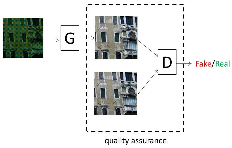
Figure 1: Introducing GAN as a strategy of quality assurance in JDD.

The key contributions of this work are summarized as follows:

$\bullet$ We have developed a GAN-based approach toward joint demosacing and denoising (JDD) in which a discriminator network with both perceptual and adversarial loss functions are used for quality assurance. Our generative network is based on deep residue learning (similar to that of [28]) but with the introduction of discriminator network, we show GAN-based JDD is capable of delivering perceptually enhanced reconstruction results;

$\bullet$ We propose to optimize the perceptual quality of reconstructed images by the proposed approach in an end-to-end manner and demonstrate its superiority to other competing methods. Such end-to-end optimization of generative and discriminator networks is particularly effective for jointly exploiting the gain brought by each modular component (e.g., residue learning in a generative network and perceptual loss in a discriminator network).

$\bullet$ Our extensive experimental results have shown convincingly superior performance over existing state-of-the-art methods in terms of both subjective and objective quality metrics with a comparable computational cost (to that of [27] and [28]). Subjective quality improvement is even more impressive for images containing fine-detailed structures (e.g., sharp edges and vivid textures).

The rest of the paper is organized below. In Sec. II, we formulate the problem of JDD and discuss some motivation behind. In Sec. III, we present the proposed GAN-based joint demosaicing and denoising approach and elaborate the issues related to network architecture, loss function and end-to-end optimization. In Sec. IV, we report our experimental results and compare them against several other competing approaches. We draw some conclusions about this research in Sec. V.

II Problem Formulation and Motivation

As mentioned in [27], demosaicing and denoising are often treated as two separated problems and studied by different communities. In practice, raw CFA data are often contaminated by sensor noise [33], which could lead to undesirable artifacts in reconstructed images if unattended. Ad-hoc sequential approaches concatenating two operations often fail: 1) denoising before demosaicing is difficult due to unknown noise characteristics and aliasing introduced by the CFA; denoising after demosaicing is challenging as well because interpolating CFA would complicate the noise behavior in the spatial domain (e.g., becoming signal-dependent). Therefore, joint demosaicing and denoising (JDD) has been conceived a more appropriate way of problem formulation. Since both demosaicing and denoising are ill-posed, a common model-based image prior can be introduced to facilitate the solution to JDD; various mathematical models have been developed - e.g. [34, 35, 36, 6, 37, 38].

Data-driven approaches toward JDD also exist in the literature such as [39, 40, 27]. Among them, [27] represents the latest advance in which a deep neural network is trained using a large corpus of images. Despite those progress, we argue that there is a fundamental issue that has been largely overlooked before - visual quality evaluation for JDD. In previous works, subjective or objective (e.g., PSNR and SSIM) quality assessment was outside the optimization loop (open-loop formulation). By contrast, it will be desirable to pursue a closed-loop formulation in which the quality of reconstructed images can be fed back to the demosaicing process. Along this line of reasoning, it is natural to connect with a recently developed tool called Generative Adversarial Networks (GAN) [30].

II-A Why Generative Adversarial Networks (GAN)?

The basic idea of GAN is to formulate a minimax two-player game by concatenating two competing networks (a generative and a discriminative). In the original setting, the generative model G captures the data distribution and the discriminative model D estimates whether a sample is from the model distribution or the data distribution (real vs. fake). Later GAN was successfully leveraged to the application of image super-resolution producing photo-realistic images [25], which inspires us to reapply GAN into image demosaicing. In the setting of image super-resolution or demosaicing, the goal of the generator is to fool the discriminator by generating perceptually convincing samples that can not be distinguished from the real one; while the goal of discriminator is to distinguish the real ground-truth images from those produced by the generator. Through the competition between generator and discriminator, we can pursue a closed-form optimization of image demosaicing. Such a minimax two-player game can be written as follows:

$$\begin{split}\mathop{min}\limits_{G}\mathop{min}\limits_{D}V(D_{\Theta_{D}}&,G_{\Theta_{G}})=E_{x\sim P_{data}(x)}\left[logD_{\Theta_{D}}(x)\right]+\\ &E_{z\sim P_{z}(z)}\left[log(1-D_{\Theta_{D}}(G_{\Theta_{G}}(z))\right]).\end{split}$$ (1)

where $P_{data}$ is the data distribution (real), $P_{z}$ is the model distribution (fake), $z$ is the input, $x$ is the label (real or fake).

GAN has received increasingly more attention in recent years. Despite its capability of generating images of good perceptual quality, GAN is also known for its weakness such as difficulty of training (e.g., mode collapse, vanishing gradients etc.), which often results in undesirable artifacts in the reconstructed images. To overcome this difficulty, a set of constraints on network topology was proposed in [41] to address the issue of instability; a conditional version of generative adversarial nets was constructed in [42] by simply feeding the labeled data, which is shown to facilitate the learning of the generator. In [43], an energy-based Generative Adversarial Network(EBGAN) views the discriminator as an energy function and exhibits more stable behavior than regular GANs during training; in [44], the Earth-Mover (EM) distance or Wasserstein distance was introduced to GAN which can effectively improve the stability of learning. Most recently, [45] proposed an alternative to clipping weights of Wasserstein GAN (WGAN): penalize the norm of gradient of the critic with respect to its input. This enables stable training for a wide variety of GAN architectures with almost no hyperparameter tuning. All these advances are positive evidence for the wider adoption of GAN in various application scenarios (style transfer [46], de-rain [32], deblur [31]).

II-B Why End-to-End Optimization?

In conventional model-based approaches, global optimization over several unknown variables is often difficult; compromised strategies such as alternating optimization are necessary. For instance, a sequential energy minimization technique was developed for JDD problem in [40] in which all hyper-parameters have to be optimized during training. As noise characteristics or CFA pattern varies, hand-crafted parameters often easily fail. By contrast, data-driven deep neural network based approach offers a convenient approach toward end-to-end optimization - i.e., instead of pursuing analytical solution to a global optimization problem, we target at learning a nonlinear mapping from the space of input images to that of output images. Such nonlinear mapping implemented by the generative network can represent arbitrary composition of image degradation processes such as down-sampling, blurring and noise contamination. From this perspective, JDD can be viewed as a special case of end-to-end optimization that could involve multiple stages of image degradation. We note that such end-to-end optimization is simply intractable in model-based formulation because the corresponding global optimization problem defies analytical solutions.

End-to-end optimization has found successful applications in robotics [47], image dehazing [48] and image compression [49]. End-to-end optimization can be implemented in either open-loop (e.g., Rate-Distortion optimization in image compression [49]) or closed-loop (e.g., vision-based motor control in robotics [47]). In the scenario of JDD, the adoption of GAN allows us to feed the perceptual difference (produced by discriminator) back to the generator, which forms a closed-loop optimization. When compared against previous deep learning-based approach toward JDD (e.g., [27]), we argue that our GAN-based end-to-end optimization has the advantage of learning the demosaicing process in a supervised manner and therefore is capable of delivering reconstructed images with guarantee of perceptual qualities.

III GAN-based Joint Demosaicing and Denoising

The problem of joint demosaicing and denoising (JDD) can be formulated as an ill-posed inverse problem in which the forward degradation process is characterized by:

$$y=F\odot x+n.$$ (2)

where $x$ is the original full-resolution color image, $F$ is 3-dimensional binary matrix indicating missing values in Bayer pattern, $\odot$ denotes element-wise multiplication, $n$ is the vector representing additive noise and $y$ is noisy CFA observation. Then JDD refers to the problem of estimating unknown $x$ from noisy and incomplete observation $y$. Due to its ill-posed nature, one has to incorporate a priori knowledge about $x$ into the solution algorithm (often called regularization). For example, in model-based approaches, we might consider the following optimization problem:

$$\mathop{min}\limits_{x}{\parallel y-F\odot x\parallel}^{2}+\lambda\parallel\rho(x)\parallel.$$ (3)

where $\rho(x)$ is a hand-crafted prior term (a.k.a. penalization function). Depending on the specific choice of $\rho$, the above optimization problem can be solved analytically (e.g., the classical Wiener filtering) or numerically (e.g., $L_{1}$-based sparse coding). It should be noted that as the degradation process becomes complicated (e.g., nonlinear degradation or non-additive noise), model-based approach simply become infeasible due to lack of tractability in theory.

Deep neural network (DNN) or deep learning based approaches offer an alternative solution to the above nonlinear inverse problem. Assuming a large amount of data is available, we can target at learning a nonlinear mapping from the space of degraded images $y$ to that of original image $x$. For the JDD problem, the goal is to estimate a full-resolution clean color image $x=I^{c}$ from a noisy input CFA image $y=I^{raw}$ (note that noise characteristics might be unknown or partially known). To learn such a nonlinear mapping (the generator network), we can train a feed-forward convolutional neural network (CNN) $G(\Theta_{G})$ parameterized by $\Theta_{G}$ where $\Theta_{G}$ is the set of parameters (weights and biases) of deep convolutional neural network. Inspired by the work of GAN [30], we introduce another discriminator network into training as an adversarial player. The goal of this discriminator network is to strive to distinguish a demosaiced image (fake) generated by the generator network from the ground truth color image (real); meanwhile the generator network attempts to fool the discriminator network by producing demosaiced image that is perceptually lossless to the ground truth. Through such a two-player game, GAN-based JDD is expected to outperform other competing approaches without the quality assurance. In the following sections, we will elaborate implementation details including network architecture, loss function and training procedure.

III-A Network Architecture

The proposed deep generator convolutional network architecture is shown in Fig. 2. It contains four convolution blocks, sixteen residual blocks(ResBlocks) as shown in Fig. 2) and one sub-pixel convolutional layer. Each ResBlocks consists of a convolution layer and a Relu activation layer. More specifically, we first use a convolution layer followed by a Relu activation layer, then sixteen ResBlocks are employed in each of which dropout regularization with a probability of $1$ is added after the first convolution layer. Next, two convolution layers and a sub-pixel convolutional layer followed. All the convolution layers are small $3\times 3$ kernels and 64 feature maps except the last one which has $64\times 4$ feature maps. Finally, in order to restore a color image which has three channels, we use a convolution layers with $3\times 3$ kernels and $3$ feature maps. In addition, we introduce a skip connection to guide the output before the sub-pixel layer.

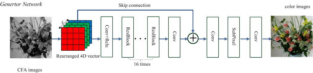
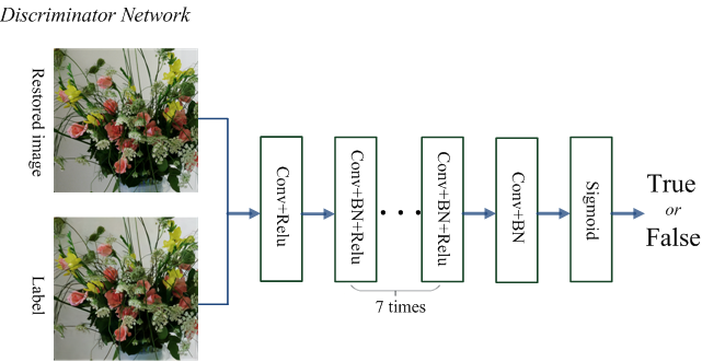
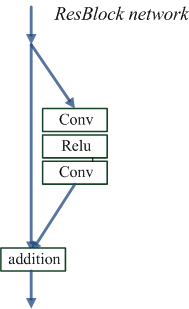
Figure 2: The architecture of our Generative adversarial networks for joint demosaicing and denoise. The top is the generator network structure. The lower left corner is the discriminator network structure. The bottom right is the structure of the residual block

To discriminate the real color image from the fake one synthesized by the generators, we have to train a discriminator network. The architecture is shown in Fig. 2. Following the structure that was proposed in [41], we propose to use a convolutional layer followed by batch normalization and LRelu activation$(\alpha=0.2)$ as the basic unit throughout the discriminator network. The network is trained to solve the two-player minmax problem in Eq. (1). It first contains $8$ convolutional layers with $3\times 3$ kernels, an increasing number of feature size by factor $2$ from $64$ to $512$ and stride $2$ is used by interval to reduce the resolution. Finally, a convolutional layer is used with $3\times 3$ kennel and feature size $1$ followed by a sigmoid activation function to gain a probability of similarity score normalized to [0,1].

III-B Loss function

The training of GAN is implemented by optimizing the following loss function:

$$\widehat{\Theta}_{G}=\mathop{argmin}\limits_{\Theta_{G}}\frac{1}{N}\sum_{n=1}^{N}L((G_{\Theta_{G}}(I^{raw}_{n}),I^{c}_{n}).$$ (4)

where $n=1,2,...,N$ and $L$ is the loss function. Pixel-wise loss functions such as MSE are known to overly smooth an image, which degrades its perceptual quality. There are two ways of improving upon such ad-hoc MSE based loss function: 1) to introduce a perceptual loss depending on high-level features for better characterizing the subjective quality of an image (often requiring a pre-trained network); 2) to introduce a discriminator network whose objective is to learn to distinguish the difference between real and fake images. In this paper, we propose to combine both ideas and formulate the following composite loss function for the problem of JDD:

$$L=L_{MSE}+\lambda_{p}L_{p}+\lambda_{A}L_{A}.$$ (5)

where $L_{MSE}$ is the conventional per-pixel loss function such as mean square error, $L_{p}$ is the perceptual loss given by a pre-trained loss network and $L_{A}$ is the adversarial loss associated with the discriminator of GAN. Two Lagrangian parameters ($\lambda_{p}$ and $\lambda_{A}$) are introduced to control the tradeoff among those three regularization terms. Detailed formulation and implementation of these three loss functions are provided as follows.

MSE loss Given an image pair ${I^{input},I^{c}}$ with width $W$ and height $H$, so is the input image $I^{input}$ with a size of $4\times H\times W$ which is a rearrangement of $I^{raw}$ , $I^{c}$ is the corresponding ground truth with a size of $3\times H\times W$. The MSE loss is given by:

$$L_{MSE}=\frac{1}{3WH}\sum_{c=1}^{3}\sum_{i=1}^{W}\sum_{j=1}^{H}\parallel(G_{\Theta_{G}}(I^{input}))^{c,w,h}-I^{c,w,h}\parallel.$$ (6)

where $G_{\Theta_{G}}$ is the parameters (weights and biases) of generator convolutional network.

Perceptual loss We adopted recently proposed Perceptual loss [46]. It is a simple $L2$ metric defined as the loss based on the ReLU activation layers of the pre-trained $19$ layer visual geometry group (VGG) network described in [22]. The perceptual loss term is given by:

$$L_{p}=\frac{1}{W_{i,j}H_{i,j}}\sum_{x=1}^{W_{i,j}}\sum_{y=1}^{H_{i,j}}(\phi_{i,j}(I^{c})_{x,y}-\phi_{i,j}(G_{\Theta_{G}}(I^{input}))_{x,y})^{2}.$$ (7)

where $W_{i,j}$ and $H_{i,j}$ describe the dimensions of the respective feature maps within the VGG19 network, $\phi_{i,j}$ is the feature map obtained by the j-th convolution (after activation) before the i-th max-pooling layer within the VGG19 network.

Adversarial loss Given a set of $N$ joint demosaicing and denoise images generated from the generator ${I^{output}}^{N}_{i=1}$, the adversarial loss fed back from the discriminator network to guide the generator network is defined as:

$$L_{A}=-\frac{1}{N}\sum_{i=1}^{N}log(D_{\Theta_{D}}(I^{output}_{i})).$$ (8)

where $D_{\Theta_{D}}$ is discriminator network, $\Theta_{D}$ is the parameters (weights and biases) of this discriminator network.

III-C Training Details

Now we describe the training process of the whole network. Given a training set $\{I^{input}_{i},I^{c}_{i}\}_{i=1}^{N}$ , where $I^{input}_{i}$ is a 4D vector which is a rearrangement of raw image $I^{raw}$ degraded by noise, $I^{c}_{i}$ is the ground-truth color image, and $N$ is the number of training samples, our aim is to learn a nonlinear mapping from the space of noisy Bayer pattern to that of full-resolution color image through the generator network $I^{c}_{i}=G_{\Theta_{G}}(I^{input}_{i})$. We optimize the network parameters through the loss function as Eq. (5) mentioned earlier.

We implemented all of our models using TensorFlow and the training was performed on a single NVIDIA 1080Ti GPU using a collection of $320$ thousand images. These training images are separated from the testing images and were cropped to patches sized $100\times 100$ (so the size of input data to the generator network is $50\times 50\times 4$). Since the models are based on a full convolutional network and are trained on image patches, we can apply the trained model to test images of arbitrary size. We normalize the input and output of networks to [0, 1], so the loss is calculated based on the scale of [0, 1]. In all experiments, we set the weight of perceptual loss $\lambda_{p}=1$ and the weight of adversarial loss $\lambda_{A}=0.001$. During the optimization, we alternately perform gradient descent steps between $G_{\Theta_{G}}$ and $D_{\Theta_{D}}$ using Adam algorithm [50] with $\beta_{1}=0.9$. The learning rate is set to $10^{-4}$ for both generator and discriminator networks; the batch size is set to $64$, which has shown relatively stable convergence process. The whole training process took around $6$ days on the machine.

Training data It is well known that deep learning benefits from a large number of training samples. In order to achieve better performance on the proposed GAN, we have hand selected more than $1400$ high-quality color images and further divided them into patches of size $100\times 100$ as the ground truth. Then we generate noisy Bayer patterns by adding random Gaussian white noise with the variance in the range of [0,20]. Moreover, in order to obtain more training data, we have adopted a strategy of data augmentation by flipping the patch left-to-right, upside-down and along the diagonal. This way the total amount of training data is increased by a factor of $8\times$, which leads to $320000$ training pairs for training.

Test data The McMaster and Kodak datasets are the most common test sets for image demosaicing. The Kodak datasets contains $24$ images of size $512\times 768$ derived from scanning of early film-based data sources. Despite the popularity of Kodak data set in image demosaicing community, most Kodak images contain relatively smooth edges and textures whose visual quality are not among the best based on the modern day’s criterion. By contrast, the McMaster data set contains $18$ images of size $500\times 500$ containing abundant strong and sharp image structures. Most recently, a new data set called Waterloo Exploration Database (WED) [51] with 4,744 high-quality natural images has been made publicly available and adopted by a recent demosaicing study [28].

IV Experimental Results

In this section, we report experimental results with the proposed method. The following objective quality measures are used to evaluate the performance of different competing methods: Color Peak Signal to Noise Ratio (CPSNR) and Structural Similarity Index (SSIM).

We have compared the proposed GAN method with several state-of-the-art joint denoise and demosaicing methods including Sequential Energy Minimization(SEM)[40], a flexible camera image processing framework (FlexISP)[38], a deep learning method(DJ)[27] and a variant of ADMM[52]and our generator network without discriminator, using their source code on the same dataset. Unlike those benchmark methods requiring the prior knowledge about the noise level of Gaussian noise, our method is blind denoise and demosaicing (no such prior is needed). Table I show the PSNR and SSIM comparisons on the Kodak dataset with noise level $\sigma=20$ and Table II show the PSNR and SSIM results on the McMaster dataset with noise level $\sigma=20$. The OURS¹ in the table represents the result of our generator network without the discriminator and the OURS² in the table represents the result of our complete GAN network (with the discriminator). It can be concluded that the objective performance of our methods are significantly better than that of benchmark methods in most situations.

We have changed the noise level of Bayer input images to different settings: $\sigma=0$ , $\sigma=5$, $\sigma=10$ and $\sigma=20$. Note that the results for noise level being zero means the JDD problem degenerates to the original demosaicing problem. The average PSNR/CPSNR and SSIM results on Kodak and McMaster are shown in Table III. Similar to [28], we have compared the PSNR result of each color channel in the table. It can be seen that the proposed method achieves much better average PSNR/CPNSR and SSIM results than all other competing methods. On the average, our method outperforms the second best method by $4.4dB$, $2.3dB$, $4.1dB$ and $1.5dB$ on four different noise levels respectively. In other words, the proposed method is much more robust to the variation of noise levels.

TABLE I: Kodak per image results(PSNR and SSIM) on noise level $\sigma=20$. The best is in bold.

Images	FlexISP	SEM	DJ	ADMM	OURS1	OURS2
1	23.13 0.5917	22.75 0.6030	26.99 0.7823	27.07 0.7687	28.06 0.8199	28.02 0.8209
2	25.69 0.4829	22.78 0.3426	30.13 0.7595	30.49 0.7741	31.43 0.7994	31.50 0.8051
3	26.63 0.4980	22.91 0.3074	31.40 0.8339	31.70 0.8590	33.31 0.8922	33.46 0.8956
4	26.01 0.5114	22.88 0.3606	30.15 0.7764	30.33 0.7969	31.38 0.8216	31.39 0.8231
5	23.58 0.6402	22.88 0.6113	27.08 0.8157	27.30 0.8211	28.69 0.8617	28.69 0.8628
6	24.79 0.5832	23.10 0.5089	28.07 0.7950	27.98 0.7895	29.34 0.8309	29.29 0.8340
7	25.66 0.5651	23.04 0.4139	30.64 0.8610	31.08 0.8967	32.59 0.9188	32.62 0.9193
8	23.35 0.6930	22.78 0.6591	26.82 0.8328	26.41 0.8297	28.50 0.8714	28.50 0.8725
9	25.85 0.5173	22.79 0.3368	31.31 0.8405	31.32 0.8710	33.02 0.8897	32.98 0.8913
10	26.17 0.5233	22.84 0.3489	30.97 0.8196	31.12 0.8532	32.85 0.8777	32.87 0.8802
11	24.95 0.5351	23.02 0.4403	28.90 0.7728	29.13 0.7805	30.19 0.8122	30.23 0.8191
12	25.90 0.4963	23.19 0.3372	31.14 0.7947	31.26 0.8189	32.66 0.8398	32.78 0.8453
13	22.22 0.5969	22.76 0.6552	25.27 0.7466	25.47 0.7189	26.38 0.7870	26.37 0.7870
14	24.27 0.5629	22.82 0.5039	27.74 0.7593	27.96 0.7631	29.04 0.7979	29.03 0.8002
15	26.09 0.5256	23.68 0.3787	30.11 0.8074	29.65 0.8239	31.79 0.8481	31.83 0.8512
16	26.07 0.5148	22.93 0.3815	29.98 0.7882	29.90 0.7917	31.16 0.8304	31.11 0.8338
17	26.01 0.5469	23.34 0.3917	30.46 0.8234	30.73 0.8378	31.89 0.8635	31.90 0.8645
18	24.48 0.5586	22.91 0.4911	27.48 0.7696	27.75 0.7694	28.68 0.8106	28.65 0.8108
19	25.28 0.5531	22.94 0.4376	29.54 0.7992	29.30 0.7995	30.80 0.8360	30.83 0.8391
20	26.24 0.6032	24.27 0.4612	29.54 0.8567	28.66 0.8633	32.71 0.8802	32.76 0.8854
21	24.95 0.5514	22.72 0.4324	28.62 0.8195	28.89 0.8407	29.94 0.8655	29.95 0.8664
22	25.41 0.5204	22.83 0.4145	28.74 0.7516	29.02 0.7632	29.89 0.7924	29.93 0.7964
23	26.71 0.5030	23.08 0.3074	31.70 0.8387	32.17 0.8769	33.77 0.9011	33.87 0.9010
24	24.14 0.5745	22.79 0.4939	27.30 0.7925	27.43 0.8082	28.83 0.8439	28.82 0.8460
AVG	25.15 0.5520	23.00 0.4425	29.17 0.8015	29.26 0.8132	30.70 0.8455	30.74 0.8479

TABLE II: McMaster per image results(PSNR and SSIM) on noise level $\sigma=20$. The best is in bold.

Images	FlexISP	SEM	DJ	ADMM	OURS1	OURS2
1	22.16 0.5864	21.42 0.5291	24.78 0.7186	25.51 0.7569	26.64 0.7967	26.74 0.7998
2	25.08 0.5650	23.57 0.4394	28.32 0.7612	28.74 0.7751	29.94 0.828	29.94 0.8312
3	22.91 0.6085	23.83 0.3941	26.61 0.8096	26.96 0.8308	28.2 0.8809	28.25 0.8826
4	24.30 0.6481	22.67 0.3639	29.04 0.8819	28.89 0.9119	31.14 0.9244	31.17 0.9261
5	24.24 0.5577	22.44 0.2670	27.85 0.7723	28.59 0.8093	29.71 0.8413	29.76 0.8433
6	24.93 0.5459	23.47 0.3513	28.77 0.7661	29.75 0.8166	30.53 0.8426	30.57 0.8449
7	25.62 0.5647	24.02 0.3696	28.44 0.7478	28.62 0.7434	29.61 0.81	29.63 0.8134
8	25.75 0.5083	22.54 0.5325	29.41 0.7258	29.26 0.7165	31.82 0.8834	31.92 0.8834
9	24.85 0.5421	22.59 0.4896	29.21 0.8090	29.81 0.8449	31.21 0.8813	31.20 0.8800
10	25.56 0.5502	23.34 0.5196	29.68 0.7958	30.07 0.8113	31.62 0.8699	31.64 0.8719
11	26.24 0.5229	23.25 0.4579	30.00 0.7636	30.31 0.7789	32.1 0.8535	32.11 0.8537
12	26.11 0.5307	22.59 0.5659	30.57 0.8391	31.29 0.8775	32.74 0.9079	32.77 0.9082
13	26.99 0.4819	23.03 0.5305	32.74 0.8434	34.04 0.8962	35.19 0.9084	35.28 0.9100
14	26.85 0.5290	22.17 0.4368	31.11 0.8122	31.62 0.8348	33.13 0.875	33.20 0.8759
15	26.64 0.5174	22.12 0.3933	30.85 0.7820	31.15 0.7968	32.97 0.8593	32.99 0.8587
16	24.42 0.6121	23.32 0.4809	26.44 0.7164	27.03 0.7366	28.36 0.8066	28.32 0.8072
17	22.80 0.5217	24.33 0.4072	26.35 0.7051	27.42 0.7586	28.28 0.7966	28.33 0.8000
18	24.80 0.6084	23.11 0.4183	28.07 0.7706	28.50 0.7862	29.97 0.8308	30.00 0.8387
AVG	25.01 0.5556	22.99 0.4415	28.79 0.7789	29.31 0.8046	30.73 0.8554	30.77 0.8572

TABLE III: Average PSNR(dB) and SSIM comparisons for the joint demosaicing and denoise results. The best is in bold.

Method	Kodak					McMaster					WED
	RPSNR	GPSNR	BPSNR	CPSNR	SSIM	RPSNR	GPSNR	BPSNR	CPSNR	SSIM	RPSNR	GPSNR	BPSNR	CPSNR	SSIM
	n=0
FlexISP	34.30	36.30	34.35	34.98	0.9426	35.18	37.39	33.00	35.19	0.9385	35.03	37.88	34.11	35.68	0.9476
SEM	37.03	40.26	36.45	37.55	0.9691	33.53	36.69	33.16	34.13	0.9301	33.98	37.84	33.77	34.75	0.9534
DJ	33.86	34.78	33.01	33.88	0.9271	32.40	34.52	30.52	32.48	0.8876	32.63	34.82	31.33	32.93	0.9174
ADMM	30.94	33.16	30.80	31.63	0.8873	31.97	34.72	31.30	32.66	0.9052	31.37	33.47	30.62	31.82	0.9075
CNNCDM	41.38	44.85	41.04	42.04	0.9882	39.14	42.10	37.31	38.98	0.9700	39.01	43.04	38.54	39.67	0.9805
OURS1	42.37	45.38	41.32	42.64	0.9894	39.37	42.26	37.48	39.17	0.9706	39.72	43.40	39.08	40.23	0.9827
OURS2	42.20	45.47	41.29	42.57	0.9889	39.29	42.44	37.49	39.17	0.9706	39.61	43.70	39.05	40.23	0.9826
Method	n=5
	RPSNR	GPSNR	BPSNR	CPSNR	SSIM	RPSNR	GPSNR	BPSNR	CPSNR	SSIM	RPSNR	GPSNR	BPSNR	CPSNR	SSIM
FlexISP	30.78	32.01	31.15	31.31	0.8694	30.86	32.45	30.23	31.18	0.8627	30.84	32.37	30.05	31.09	0.8701
SEM	34.04	35.60	34.38	34.59	0.9269	31.68	33.89	31.95	32.36	0.8869	32.07	34.48	32.27	32.74	0.9114
DJ	32.93	33.82	32.48	33.08	0.9058	31.86	33.79	30.38	32.01	0.8739	31.99	34.01	31.00	32.33	0.8983
ADMM	31.19	32.41	31.20	31.60	0.8787	32.33	33.90	31.65	32.63	0.8966	31.69	32.69	30.99	31.79	0.8955
OURS1	36.72	37.64	36.42	36.87	0.9506	35.97	37.23	34.94	35.87	0.9387	35.67	37.53	35.21	35.94	0.9539
OURS2	36.66	37.58	36.37	36.82	0.9506	35.94	37.18	34.96	35.86	0.9386	35.61	37.45	35.19	35.90	0.9538
Method	n=10
	RPSNR	GPSNR	BPSNR	CPSNR	SSIM	RPSNR	GPSNR	BPSNR	CPSNR	SSIM	RPSNR	GPSNR	BPSNR	CPSNR	SSIM
FlexIS	28.32	28.81	28.78	28.64	0.7583	28.25	29.13	28.16	28.51	0.7534	28.12	28.92	27.69	28.24	0.7603
SEM	29.22	29.97	30.26	29.78	0.7681	27.90	29.38	28.98	28.68	0.7306	28.20	29.61	29.02	28.87	0.7587
DJ	31.45	32.19	31.32	31.65	0.8731	30.79	32.34	29.72	30.95	0.8467	30.78	32.42	30.05	31.08	0.8668
ADMM	30.72	31.47	30.92	31.04	0.8595	31.57	32.53	31.07	31.72	0.8699	31.02	31.58	30.51	31.04	0.8714
OURS1	33.67	34.30	33.70	33.87	0.9125	33.57	34.45	33.08	33.60	0.9092	33.28	34.60	32.91	33.47	0.9260
OURS2	33.68	34.28	33.67	33.86	0.9129	33.58	34.46	33.08	33.61	0.9097	33.27	34.57	32.92	33.46	0.9266
Method	n=20
	RPSNR	GPSNR	BPSNR	CPSNR	SSIM	RPSNR	GPSNR	BPSNR	CPSNR	SSIM	RPSNR	GPSNR	BPSNR	CPSNR	SSIM
FlexIS	25.13	24.69	25.62	25.15	0.5520	24.95	24.99	25.10	25.01	0.5556	24.88	24.77	24.74	24.80	0.5695
SEM	22.46	23.01	23.65	23.00	0.4425	22.11	23.34	23.74	23.0	0.4415	22.26	23.22	23.45	22.93	0.4605
DJ	28.94	29.49	29.08	29.17	0.8015	28.61	29.73	28.03	28.79	0.7789	28.48	29.67	28.04	28.73	0.8012
ADMM	29.01	29.39	29.37	29.26	0.8132	29.24	29.81	28.88	29.31	0.8046	28.85	29.22	28.52	28.87	0.8197
OURS1	30.48	30.98	30.70	30.70	0.8455	30.55	31.32	30.56	30.73	0.8554	30.33	31.33	30.10	30.49	0.8747
OURS2	30.50	30.99	30.72	30.73	0.8479	30.60	31.34	30.59	30.77	0.8572	30.35	31.33	30.13	30.52	0.8767

Figs.3-10 demonstrates the subjective quality comparison results with a noise level of $\sigma=20$. We observe that the method of SEM suffers from lack of robustness to noise; the methods of FlexISP and DeepJoint both suffer from various artifacts such as vertical color lines, leftover noisy pixels and unnatural color. Among the competing approaches, the ADMM algorithm is relatively good, but when compared with our method still arguably falls behind in terms of visual quality. The reconstructed images by our method visually appear much better in terms of fewer artifacts, better preserved fine details (e.g., flower petals, wood texture patterns and hairs) and more vivid color demonstrating the superiority and robustness of the proposed algorithm.

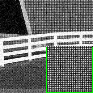
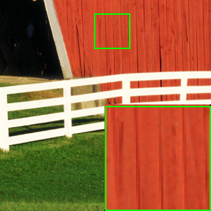
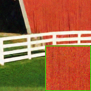
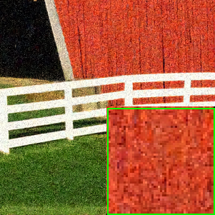
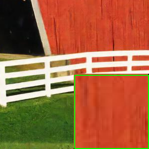
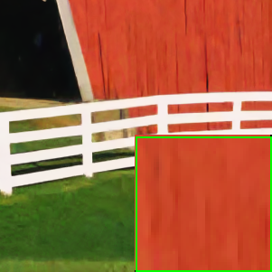
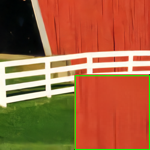
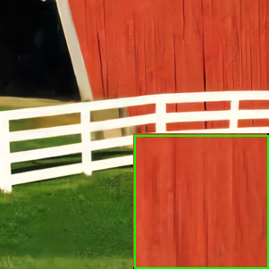
Figure 3: Visual Results of McMaster18 with $\sigma=20$ noise for Joint denoising and demosaicking. (a) BayerNoisy image; (b) Original image; (c) FlexISP result(PSNR=24.80, SSIM=0.6084); (d) SEM result(PSNR=23.11, SSIM=0.4183); (e) DeepJoint result(PSNR=28.07, SSIM=0.7706); (f) ADMM result(PSNR=28.50, SSIM=0.7862); (g) our generator network result(PSNR=29.97, SSIM=0.8308); (h) our GAN result(PSNR=30.00, SSIM=0.8387).

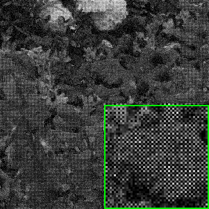
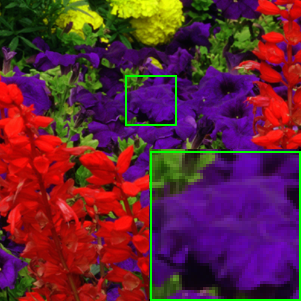
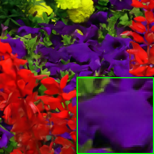
Figure 4: Visual Results of McMaster17 with $\sigma=20$ noise for Joint denoising and demosaicking. (a) BayerNoisy image; (b) Original image; (c) FlexISP result(PSNR=22.80, SSIM=0.5217); (d) SEM result(PSNR=24.33, SSIM=0.4072); (e) DeepJoint result(PSNR=26.35, SSIM=0.7051); (f) ADMM result(PSNR=27.42, SSIM=0.7586); (g) our generator network result(PSNR=28.28, SSIM=0.7966); (h) our GAN result(PSNR=28.33, SSIM=0.8000).

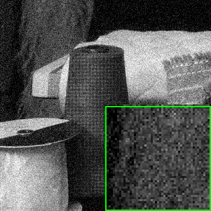
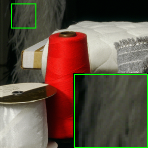
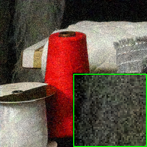
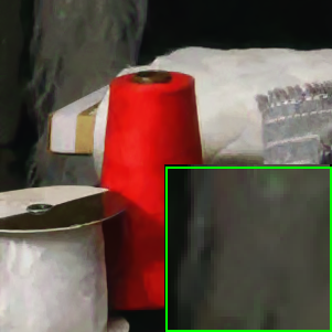
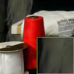
Figure 5: Visual Results of McMaster7 with $\sigma=20$ noise for Joint denoising and demosaicking. (a) BayerNoisy image; (b) Original image; (c) FlexISP result(PSNR=25.62, SSIM=0.5647); (d) SEM result(PSNR=24.02, SSIM=0.3696); (e) DeepJoint result(PSNR=28.44, SSIM=0.7478); (f) ADMM result(PSNR=28.62, SSIM=0.7434); (g) our generator network result(PSNR=29.61, SSIM=0.81); (h) our GAN result(PSNR=29.63, SSIM=0.8134).

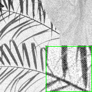
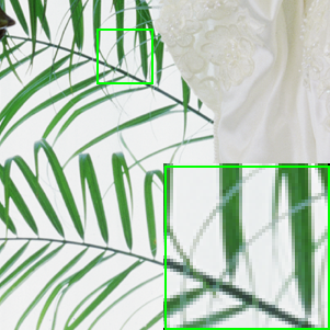
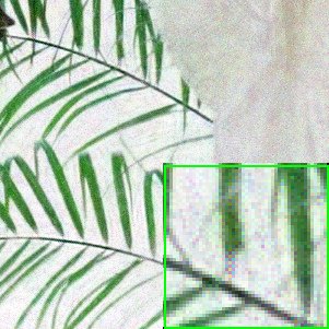
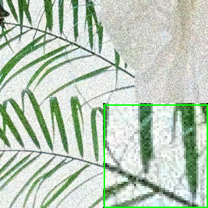
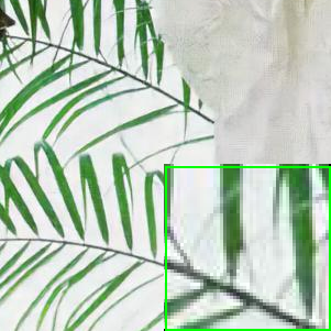
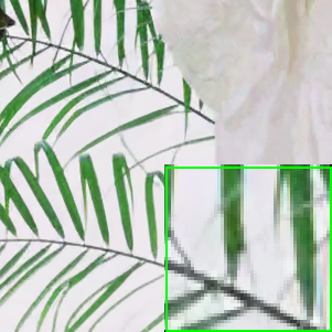
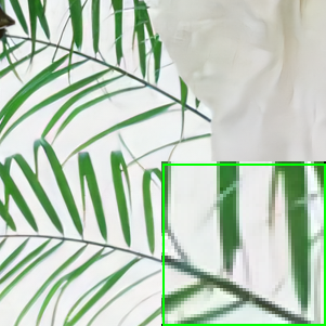
Figure 6: Visual Results of McMaster4 with $\sigma=20$ noise for Joint denoising and demosaicking. (a) BayerNoisy image; (b) Original image; (c) FlexISP result(PSNR=24.30, SSIM=0.6481); (d) SEM result(PSNR=22.67, SSIM=0.3639); (e) DeepJoint result(PSNR=29.04, SSIM=0.8819); (f) ADMM result(PSNR=28.89, SSIM=0.9119); (g) our generator network result(PSNR=31.14, SSIM=0.9244); (h) our GAN result(PSNR=31.17, SSIM=0.9261).

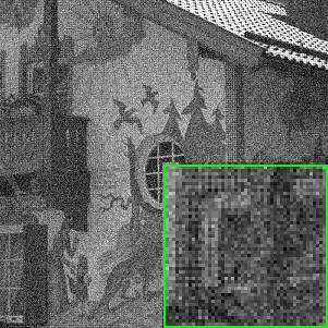
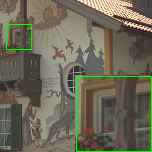
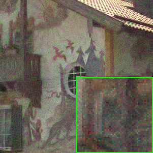
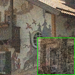
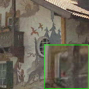
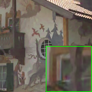
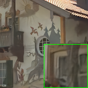
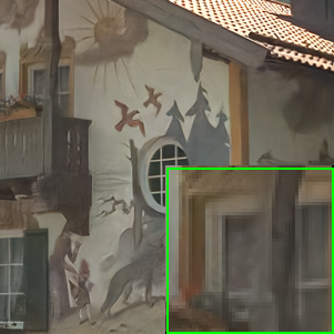
Figure 7: Visual Results of kodak24 with $\sigma=20$ noise for Joint denoising and demosaicking. (a) BayerNoisy image; (b) Original image; (c) FlexISP result(PSNR=24.14, SSIM=0.5745); (d) SEM result(PSNR=22.79, SSIM=0.4939); (e) DeepJoint result(PSNR=27.30, SSIM=0.7925); (f) ADMM result(PSNR=27.43, SSIM=0.8082); (g) our generator network result(PSNR=28.83, SSIM=0.8439); (h) our GAN result(PSNR=28.82, SSIM=0.8460).

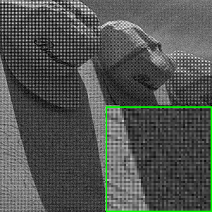
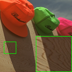
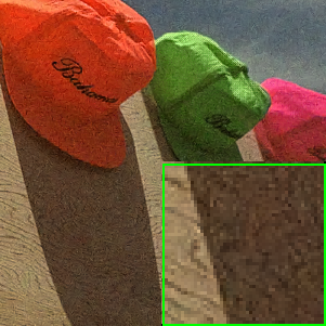
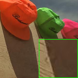
Figure 8: Visual Results of kodak3 with $\sigma=10$ noise for Joint denoising and demosaicking. (a) BayerNoisy image; (b) Original image; (c) FlexISP result(PSNR=30.90, SSIM=0.7521); (d) SEM result(PSNR=30.36, SSIM=0.6973); (e) DeepJoint result(PSNR=33.99, SSIM=0.9009); (f) ADMM result(PSNR=33.40, SSIM=0.8949); (g) our generator network result(PSNR=36.51, SSIM=0.9362); (h) our GAN result(PSNR=36.57, SSIM=0.9370).

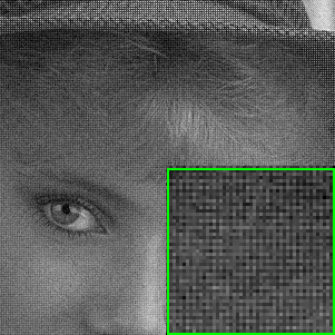
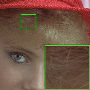
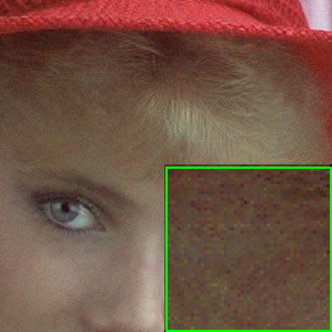
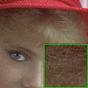
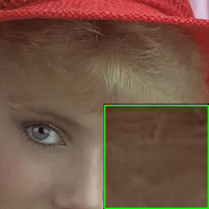
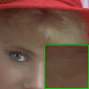
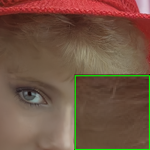
Figure 9: Visual Results of kodak4 with $\sigma=10$ noise for Joint denoising and demosaicking. (a) BayerNoisy image; (b) Original image; (c) FlexISP result(PSNR=29.67, SSIM=0.7395); (d) SEM result(PSNR=29.63, SSIM=0.7055); (e) DeepJoint result(PSNR=32.43, SSIM=0.8495); (f) ADMM result(PSNR=31.93, SSIM=0.8414); (g) our generator network result(PSNR=34.27, SSIM=0.8912); (h) our GAN result(PSNR=34.27, SSIM=0.8928).

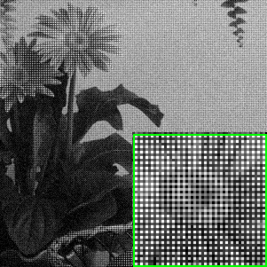
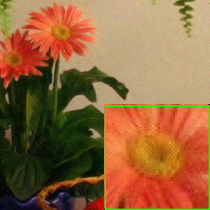
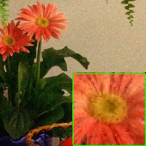
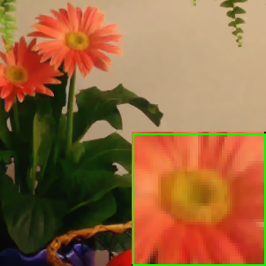
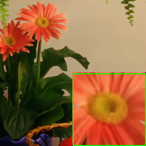
Figure 10: Visual Results of kodak9 with $\sigma=10$ noise for Joint denoising and demosaicking. (a) BayerNoisy image; (b) Original image; (c) FlexISP result(PSNR=30.53, SSIM=0.7621); (d) SEM result(PSNR=30.71, SSIM=0.7244); (e) DeepJoint result(PSNR=34.01, SSIM=0.9031); (f) ADMM result(PSNR=32.99, SSIM=0.9025); (g) our generator network result(PSNR=36.12, SSIM=0.9277); (h) our GAN result(PSNR=36.05, SSIM=0.9280).

V Conclusions

This paper presented a powerful joint demosaicing and denoise scheme based on recently-developed Generative Adversarial Network(GAN) and developed an end-to-end optimization technique using a combination of perceptual and adversarial loss functions. The introduction of discriminator network and end-to-end optimization makes it possible to achieve the quality assurance in the challenging scenario of JDD even in the presence of noise variations. The proposed GAN-based approach not only significantly improves the visual quality of reconstructed images but also keep the computational cost comparable to that of other competing approaches. A natural next step along this line of research is to test the proposed technique on some real-world noisy Bayer pattern and verify its effectiveness in practical scenario.

References

[1]
B. E. Bayer, “Color imaging array,” 1976.
[2]
L. Chang and Y. P. Tan, “Effective use of spatial and spectral correlations
for color filter array demosaicking,” Consumer Electronics IEEE
Transactions on, vol. 50, no. 1, pp. 355–365, 2004.
[3]
L. Zhang and X. Wu, “Color demosaicking via directional linear minimum mean
square-error estimation.” IEEE Transactions on Image Processing,
vol. 14, no. 12, pp. 2167–2178, 2005.
[4]
D. Paliy, V. Katkovnik, R. Bilcu, S. Alenius, and K. Egiazarian, “Spatially
adaptive color filter array interpolation for noiseless and noisy data,”
International Journal of Imaging Systems and Technology, vol. 17,
no. 3, p. 105–122, 2007.
[5]
X. Li, B. Gunturk, and L. Zhang, “Image demosaicing: a systematic survey,”
Proceedings of SPIE - The International Society for Optical
Engineering, vol. 6822, pp. 68 221J–68 221J–15, 2008.
[6]
T. Saito and T. Komatsu, “Demosaicing approach based on extended color
total-variation regularization,” in IEEE International Conference on
Image Processing, 2008, pp. 885–888.
[7]
F. Zhang, X. Wu, X. Yang, W. Zhang, and L. Zhang, “Robust color demosaicking
with adaptation to varying spectral correlations,” IEEE Transactions
on Image Processing, vol. 18, no. 12, pp. 2706–2717, 2009.
[8]
J. Mairal, F. Bach, J. Ponce, G. Sapiro, and A. Zisserman, “Non-local sparse
models for image restoration,” in IEEE International Conference on
Computer Vision, 2010, pp. 2272–2279.
[9]
D. Kiku, Y. Monno, M. Tanaka, and M. Okutomi, “Residual interpolation for
color image demosaicking,” in Image Processing (ICIP), 2013 20th IEEE
International Conference on. IEEE,
2013, pp. 2304–2308.
[10]
D. Kiku, Y. Monno, and M. Tanaka, “Minimized-laplacian residual interpolation
for color image demosaicking,” Proceedings of SPIE - The International
Society for Optical Engineering, vol. 9023, no. 1, pp. 2304 – 2308, 2014.
[11]
Y. Monno, D. Kiku, M. Tanaka, and M. Okutomi, “Adaptive residual interpolation
for color image demosaicking,” in IEEE International Conference on
Image Processing, 2015, pp. 3861–3865.
[12]
E. Gershikov, “Optimized color transforms for image demosaicing,”
International Journal of Computational Engineering Research, 2014.
[13]
R. Kimmel, “Demosaicing: Image reconstruction from color ccd samples,” in
European Conference on Computer Vision, 1998, pp. 610–622.
[14]
B. K. Gunturk, Y. Altunbasak, and R. M. Mersereau, “Color plane interpolation
using alternating projections.” IEEE Transactions on Image Processing
A Publication of the IEEE Signal Processing Society, vol. 11, no. 9, pp.
997–1013, 2002.
[15]
X. Li, “Demosaicing by successive approximation,” IEEE Transactions on
Image Processing, vol. 14, no. 3, pp. 370–379, 2005.
[16]
W. Ye and K.-K. Ma, “Color image demosaicing using iterative residual
interpolation,” IEEE Transactions on Image Processing, vol. 24,
no. 12, pp. 5879–5891, 2015.
[17]
J. Go, K. Sohn, and C. Lee, “Interpolation using neural networks for digital
still cameras,” IEEE Transactions on Consumer Electronics, vol. 46,
no. 3, pp. 610–616, 2000.
[18]
H. Z. Helor, “Demosaicking using artificial neural networks,” Proc
Spie, vol. 45, no. 3962, pp. 112–120, 2000.
[19]
F. L. He, Y. C. F. Wang, and K. L. Hua, “Self-learning approach to color
demosaicking via support vector regression,” in IEEE International
Conference on Image Processing, 2013, pp. 2765–2768.
[20]
J. Sun and M. F. Tappen, “Separable markov random field model and its
applications in low level vision,” IEEE Transactions on Image
Processing A Publication of the IEEE Signal Processing Society, vol. 22,
no. 1, p. 402, 2013.
[21]
Y. Lecun, Y. Bengio, and G. Hinton, “Deep learning,” Nature, vol. 521,
no. 7553, p. 436, 2015.
[22]
K. Simonyan and A. Zisserman, “Very deep convolutional networks for
large-scale image recognition,” Computer Science, 2014.
[23]
K. He, X. Zhang, S. Ren, and J. Sun, “Deep residual learning for image
recognition,” in Proceedings of the IEEE conference on computer vision
and pattern recognition, 2016, pp. 770–778.
[24]
Y. Taigman, M. Yang, M. Ranzato, and L. Wolf, “Deepface: Closing the gap to
human-level performance in face verification,” in Proceedings of the
IEEE conference on computer vision and pattern recognition, 2014, pp.
1701–1708.
[25]
C. Ledig, Z. Wang, W. Shi, L. Theis, F. Huszar, J. Caballero, A. Cunningham,
A. Acosta, A. Aitken, and A. Tejani, “Photo-realistic single image
super-resolution using a generative adversarial network,” pp. 105–114,
2016.
[26]
K. Zhang, W. Zuo, Y. Chen, D. Meng, and L. Zhang, “Beyond a gaussian denoiser:
Residual learning of deep cnn for image denoising,” IEEE Transactions
on Image Processing, 2017.
[27]
M. Gharbi, G. Chaurasia, S. Paris, and F. Durand, “Deep joint demosaicking and
denoising,” Acm Transactions on Graphics, vol. 35, no. 6, p. 191,
2016.
[28]
R. Tan, K. Zhang, W. Zuo, and L. Zhang, “Color image demosaicking via deep
residual learning,” in IEEE International Conference on Multimedia and
Expo, 2017, pp. 793–798.
[29]
Z. Wang, A. C. Bovik, H. R. Sheikh, and E. P. Simoncelli, “Image quality
assessment: from error visibility to structural similarity,” IEEE
transactions on image processing, vol. 13, no. 4, pp. 600–612, 2004.
[30]
I. J. Goodfellow, J. Pougetabadie, M. Mirza, B. Xu, D. Wardefarley, S. Ozair,
A. Courville, and Y. Bengio, “Generative adversarial networks,”
Advances in Neural Information Processing Systems, vol. 3, pp.
2672–2680, 2014.
[31]
O. Kupyn, V. Budzan, M. Mykhailych, D. Mishkin, and J. Matas, “Deblurgan:
Blind motion deblurring using conditional adversarial networks,” 2017.
[32]
H. Zhang, V. Sindagi, and V. M. Patel, “Image de-raining using a conditional
generative adversarial network,” 2017.
[33]
K. Hirakawa and T. W. Parks, “Joint demosaicing and denoising,” IEEE
Transactions on Image Processing, vol. 15, no. 8, pp. 2146–2157, 2006.
[34]
K. Hirakawa and X. L. Meng, “An empirical bayes em-wavelet unification for
simultaneous denoising, interpolation, and/or demosaicing,” in IEEE
International Conference on Image Processing, 2006, pp. 1453–1456.
[35]
L. Zhang, X. Wu, and D. Zhang, “Color reproduction from noisy cfa data of
single sensor digital cameras,” IEEE Transactions on Image Processing
A Publication of the IEEE Signal Processing Society, vol. 16, no. 9, pp.
2184–2197, 2007.
[36]
D. Paliy, A. Foi, R. Bilcu, and V. Katkovnik, “Denoising and interpolation of
noisy bayer data with adaptive cross-color filters,” Proceedings of
Spie the International Society for Optical Engineering, vol. 6822, no. 6822,
2010.
[37]
D. Menon and G. Calvagno, “Regularization approaches to demosaicking,”
IEEE Transactions on Image Processing A Publication of the IEEE Signal
Processing Society, vol. 18, no. 10, p. 2209, 2009.
[38]
F. Heide, O. Gallo, O. Gallo, O. Gallo, O. Gallo, O. Gallo, K. Pulli, K. Pulli,
K. Pulli, and K. Pulli, “Flexisp: a flexible camera image processing
framework,” Acm Transactions on Graphics, vol. 33, no. 6, p. 231,
2014.
[39]
D. Khashabi, S. Nowozin, J. Jancsary, and A. W. Fitzgibbon, “Joint demosaicing
and denoising via learned nonparametric random fields,” Image
Processing IEEE Transactions on, vol. 23, no. 12, pp. 4968–81, 2014.
[40]
T. Klatzer, K. Hammernik, P. Knobelreiter, and T. Pock, “Learning joint
demosaicing and denoising based on sequential energy minimization,” in
IEEE International Conference on Computational Photography, 2016, pp.
1–11.
[41]
A. Radford, L. Metz, and S. Chintala, “Unsupervised representation learning
with deep convolutional generative adversarial networks,” Computer
Science, 2015.
[42]
M. Mirza and S. Osindero, “Conditional generative adversarial nets,”
Computer Science, pp. 2672–2680, 2014.
[43]
J. Zhao, M. Mathieu, and Y. Lecun, “Energy-based generative adversarial
network,” 2016.
[44]
M. Arjovsky, S. Chintala, and L. Bottou, “Wasserstein gan,” 2017.
[45]
I. Gulrajani, F. Ahmed, M. Arjovsky, V. Dumoulin, and A. Courville, “Improved
training of wasserstein gans,” 2017.
[46]
J. Johnson, A. Alahi, and F. F. Li, “Perceptual losses for real-time style
transfer and super-resolution,” pp. 694–711, 2016.
[47]
S. Levine, C. Finn, T. Darrell, and P. Abbeel, “End-to-end training of deep
visuomotor policies,” Journal of Machine Learning Research, vol. 17,
no. 39, pp. 1–40, 2016.
[48]
B. Cai, X. Xu, K. Jia, C. Qing, and D. Tao, “Dehazenet: An end-to-end system
for single image haze removal,” IEEE Transactions on Image
Processing, vol. 25, no. 11, pp. 5187–5198, 2016.
[49]
J. Ballé, V. Laparra, and E. P. Simoncelli, “End-to-end optimized image
compression,” arXiv preprint arXiv:1611.01704, 2016.
[50]
D. P. Kingma and J. Ba, “Adam: A method for stochastic optimization,”
arXiv preprint arXiv:1412.6980, 2014.
[51]
K. Ma, Z. Duanmu, Q. Wu, Z. Wang, H. Yong, H. Li, and L. Zhang, “Waterloo
exploration database: New challenges for image quality assessment models,”
IEEE Transactions on Image Processing, vol. 26, no. 2, pp. 1004–1016,
2017.
[52]
H. Tan, X. Zeng, S. Lai, Y. Liu, and M. Zhang, “Joint demosaicing and
denoising of noisy bayer images with admm,” in IEEE International
Conference on Image Processing, 2017.