An X-ray Imaging Survey of Quasar Jets – The Complete Survey

Abstract

We present Chandra X-ray imaging of a flux-limited sample of flat spectrum radio-emitting quasars with jet-like structure. X-rays are detected from 59% of 56 jets. No counterjets were detected. The core spectra are fitted by power law spectra with photon index $\Gamma_{x}$ whose distribution is consistent with a normal distribution with mean $1.61^{+0.04}_{-0.05}$ and dispersion $0.15^{+0.04}_{-0.03}$. We show that the distribution of $\alpha_{rx}$, the spectral index between the X-ray and radio band jet fluxes, fits a Gaussian with mean 0.974$\pm$0.012 and dispersion 0.077 $\pm$ 0.008. We test the model in which kpc-scale X-rays result from inverse Compton scattering of cosmic microwave background photons off the jet’s relativistic electrons (the IC-CMB model). In the IC-CMB model, a quantity $Q$ computed from observed fluxes and the apparent size of the emission region depends on redshift as $(1+z)^{3+\alpha}$. We fit $Q\propto(1+z)^{a}$, finding $a=0.88\pm 0.90$ and reject at 99.5% confidence the hypothesis that the average $\alpha_{rx}$ depends on redshift in the manner expected in the IC-CMB model. This conclusion is mitigated by lack of detailed knowledge of the emission region geometry, which requires deeper or higher resolution X-ray observations. Furthermore, if the IC-CMB model is valid for X-ray emission from kpc-scale jets, then the jets must decelerate on average: bulk Lorentz factors should drop from about 15 to 2-3 between pc and kpc scales. Our results compound the problems that the IC-CMB model has in explaining the X-ray emission of kpc-scale jets.

1 Introduction

The pc-scale jets of powerful quasars are highly relativistic, with bulk Lorentz factors ($\Gamma=(1-\beta^{2})^{-1/2}$) of 10-30 (Cohen et al., 2007; Lister et al., 2009a). Since radio galaxies and quasars are generally double lobed, the jets that deliver energy to the lobes, hundreds of kpc from the core, must also be two sided. Because many radio jets, and practically all of those emitting X-rays, appear to be one-sided, most models of kpc-scale jets invoke bulk relativistic motion, with beaming factors, $\delta=1/(\Gamma[1-\beta\cos\theta])>\,$1, where $\theta$ is the angle of the jet to the line of sight.

On kpc scales, many fundamental physical properties of quasar jets remain uncertain, such as the proton or positron content, whether the particle and magnetic field energy densities are near equipartition, and whether the jets have high $\Gamma$ tens to hundreds of kpc from the quasar core. All of these issues bear on the flux of useful energy carried by the jet. The jets typically carry a significant fraction of the quasar energy budget, and therefore potentially provide information about the fueling and rate of growth of the central black hole. Chandra snapshot surveys (Sambruna et al., 2004; Marshall et al., 2005, 2011) have shown that X-rays are easily detected from most radio jets in quasars. One-zone (single population) synchrotron and synchrotron self-Compton (SSC) models generally fail to explain the emission, as found in the first Chandra observation of the kpc scale jet emanating from the quasar PKS 0637$-$752 (Schwartz et al., 2000) and noted in many subsequent observations of individual sources. For a review, see Harris & Krawczynski (2006) and Worrall (2009).

Due to the failure of single-zone synchrotron models, the X-ray emission of kpc-scale quasar jets is usually interpreted as inverse Compton emission of relativistic jet electrons off cosmic microwave background photons (IC-CMB). This requires that the jet emission is Doppler boosted with large Lorentz factor $\Gamma$, and at a small angle, $\theta$, to the line of sight (Tavecchio et al., 2000; Celotti et al., 2001). The IC-CMB emission is brighter than self-Compton emission because the CMB energy density is enhanced by a factor $\Gamma^{2}$ in the jet rest frame. The model was used to explain the discovery observations of PKS 0637$-$752 and was subsequently invoked often to explain bright X-ray knots in individual sources as well as for jet surveys (Sambruna et al., 2004; Marshall et al., 2005; Jorstad & Marscher, 2006; Marshall et al., 2011; Hogan et al., 2011). If valid, the model can be used to compute the jet speed along the flow to deduce bulk deceleration (Georganopoulos & Kazanas, 2004; Marshall et al., 2006; Hardcastle, 2006), or to infer that matter is entrained (Tavecchio et al., 2006).

In the past 10-15 years, however, there have been concerns that the IC-CMB model is inadequate or even rejected in some jets (Kataoka & Stawarz, 2005; Hardcastle, 2006; Jester et al., 2006). One concern with the IC-CMB model is that the lifetimes of the electrons responsible for the X-ray emission are orders of magnitude longer than those producing the radio emission so the X-ray structures would be expected to extend further downstream than the radio; just the opposite of what is regularly observed (Tavecchio et al., 2003; Schwartz et al., 2006). Of particular interest is the observation that $\gamma$-ray emission expected in the IC-CMB model (Meyer & Georganopoulos, 2014; Meyer et al., 2015, 2017; Breiding et al., 2017) is not detected, even for PKS 0637$-$752, the prototypical case for the IC-CMB model. An alternative class of models proposes additional synchrotron components to explain the X-rays (Stawarz et al., 2004; Jester et al., 2006; Hardcastle, 2006). Either model has dramatic consequences: in the IC-CMB case, jets should show surface brightnesses that are largely independent of redshift (Schwartz, 2002); while synchrotron models require electrons to be accelerated to Lorentz factors $\sim$ 10⁷ over much or all of the jet, due to their short lifetimes.

In order to find good cases for detailed study, we started a large, shallow survey using Chandra to find X-ray emission from kpc-scale radio jets. This paper is a continuation of Marshall et al. (2005, hereafter, Paper I) and Marshall et al. (2011, hereafter, Paper II) and presents observations of the remainder of the quasars from the original sample of 56. We use this sample for a population test of the IC-CMB model’s primary predictions. Following Paper II and Hogan et al. (2011), we include results from VLBI observations from the MOJAVE program that indicate the directions and speeds of relativistic jets in the quasar cores. If the IC-CMB model is correct, then we may test whether the pc scale jet has changed directions or decelerated in propagating to kpc scales. We use a cosmology in which $H_{0}=70$ km s^-1 Mpc^-1, $\Omega_{\rm m}=0.3$, and $\Omega_{\Lambda}=0.7$.

2 Sample Properties

Sample selection was described in Paper I. Briefly, 56 sources were selected from 1.64 or 5 GHz VLA and ATCA imaging surveys (Murphy et al., 1993; Lovell, 1997). The dominant selection criterion is on radio core flux density – as applied when creating the samples for the radio imaging surveys. The flux densities in jet-like extended emission determine inclusion in our sample. Subsamples were defined in Paper I: the “A” list is a complete flux-limited sample based only on extended emission, while the “B” list was selected for one-sided and linear structure. There are the same number of objects in each list and flux-limited selection was applied first.

We reported results for the first 20 targets in Paper I, finding that 60% of the jets could be detected in short Chandra exposures. In Paper II, we presented results for another 19 quasars in the sample and got the same detection rate. Here, the observations of the remaining 17 quasars of the sample are presented. The radio fluxes of the extended emission in these additional targets were somewhat lower than for the first 39 but were observed for about the same X-ray exposure time (5.8 ks on average). Fourteen of the new Chandra images were obtained as part of the completion of our survey and the other three were taken from the Chandra archive. For the 14 new observations, we also obtained Hubble Space Telescope (HST) images.

As reported in Paper II, a significant fraction of the sample is being monitored with VLBI, mostly in the northern hemisphere. Superluminal motions have been detected for every object in our sample that was observed in the MOJAVE program (see table 10). As in Paper II, the distribution of the apparent velocities, $c\beta_{app}$, is comparable to those of the remaining MOJAVE sources, indicating that quasars in our sample have a distribution of speeds and line of sight angles that is consistent with that of the MOJAVE program.

Five redshifts were unknown as of Paper I. In Paper II, we reported that the redshift of PKS 1421$-$490 was 0.662. We now include PKS 1145$-$676 in our overall analysis with a redshift of 0.21 (Sbarufatti et al., 2009), PKS 0144$-$522 with a redshift of 0.098 (Schechter & Dressler, 1987), and PKS 1302$-$82, with a redshift of 0.87 (Burgess & Hunstead, 2006). As noted in Paper I, PKS 1145$-$676 shows X-ray emission from a 5″ long region. The redshift is still unknown for one object in the sample for which we have an X-ray image: PKS 1251$-$713. We excluded this source from sample analyses that require redshifts.

3 Observations and Data Reduction

The Chandra observation list is given in Table 1. As in Papers I and II, X-ray images were formed from events in the 0.5-7.0 keV band (see Fig. 1). The images of a few sources show readout streaks, which do not interfere with the jets because we selected a suitable range of observatory roll angles.

Table 1: Chandra Observation Log

Target	Chandra	Live Time	Date	Ref.
	Obs ID	(s)	(UT)
0106$+$013	9281	8787	2007-11-21	2
0144$-$522	10366	5590	2009-03-26	1
0256$+$075	10375	5604	2008-12-07	1
0402$-$362	10374	5582	2009-03-19	1
0508$-$220	10367	5294	2009-02-25	1
0707$+$476	10368	5309	2009-01-20	1
0748$+$126	10376	5610	2009-02-07	1
0833$+$585	7870	3771	2007-01-12	1
0859$+$470	10371	5604	2008-12-31	1
0953$+$254	10377	5606	2009-01-20	1
1116$+$128	10373	5579	2009-02-01	1
1303$-$827	10365	5612	2009-11-18	1
1502$+$106	10378	5608	2009-04-09	1
1622$-$297	10370	5610	2009-06-17	1
1823$+$568	10369	5578	2009-06-06	1
2201$+$315	9283	9167	2008-10-12	2
2230$+$114	10372	5450	2009-08-06	1

Table 2 lists the radio data used here and radio flux contours are overlaid on the X-ray images in Figure 1. X-ray images were registered to radio images as in Paper I.

Table 2: Radio Observations

Target	Instrument	Date	Freq.	$5\times$ RMS noise
		(UT)	(GHz)	(mJy/beam)
0106$+$013	VLA	2000-11-05	1.42	4.29
0144$-$522	ATCA	2004-05-08	17.73	0.50
0256$+$075	VLA	2000-11-05	1.42	2.64
0402$-$362	ATCA	2002-02-01	8.64	2.52
0508$-$220	ATCA	2000-11-05	1.42	8.40
0707$+$476	VLA	2000-11-05	4.86	1.34
0748$+$126	VLA	2001-05-06	4.86	1.50
0833$+$585	VLA	2000-11-05	1.42	2.44
0859$+$470	VLA	2000-11-05	4.86	2.51
0953$+$254	VLA	2000-11-05	1.42	1.93
1116$+$128	VLA	2000-11-05	4.86	1.70
1303$-$827	ATCA	1993-07-13	8.64	4.17
1502$+$106	VLA	2000-11-05	4.86	1.94
1622$-$297	ATCA	1994-07-29	8.64	9.06
1823$+$568	VLA	2000-11-05	4.86	4.32
2201$+$315	VLA	2000-11-05	1.42	2.64
2230$+$114	VLA	2000-11-05	4.86	4.09

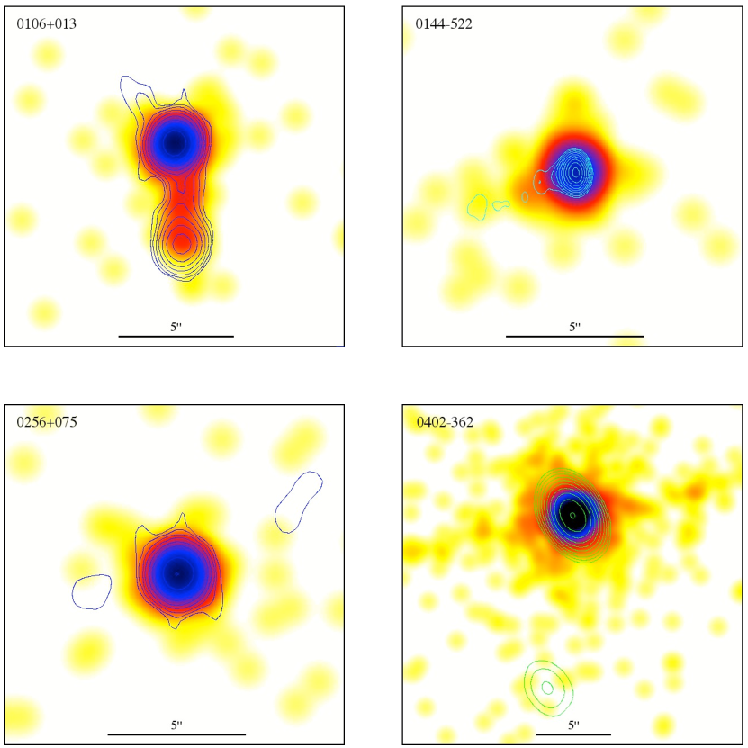
Figure 1: X-ray images from Chandra observations, with contours from Australia Telescope Compact Array or Very Large Array (VLA) images. The radio surface brightness contours increase by a factor of 2 and start at 5 times the rms noise, as given in Table 2. The X-ray images were convolved with 1″ Gaussians and then binned at 0.0492″, a tenth of a Chandra pixel. The color scale for all images is logarithmic, from 0.5 counts/beam (yellow) to 2500 counts/beam (black). See the text for comments on individual objects. A readout streak is apparent in the X-ray map of 2201$+$315.

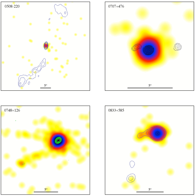
Figure 1: continued.

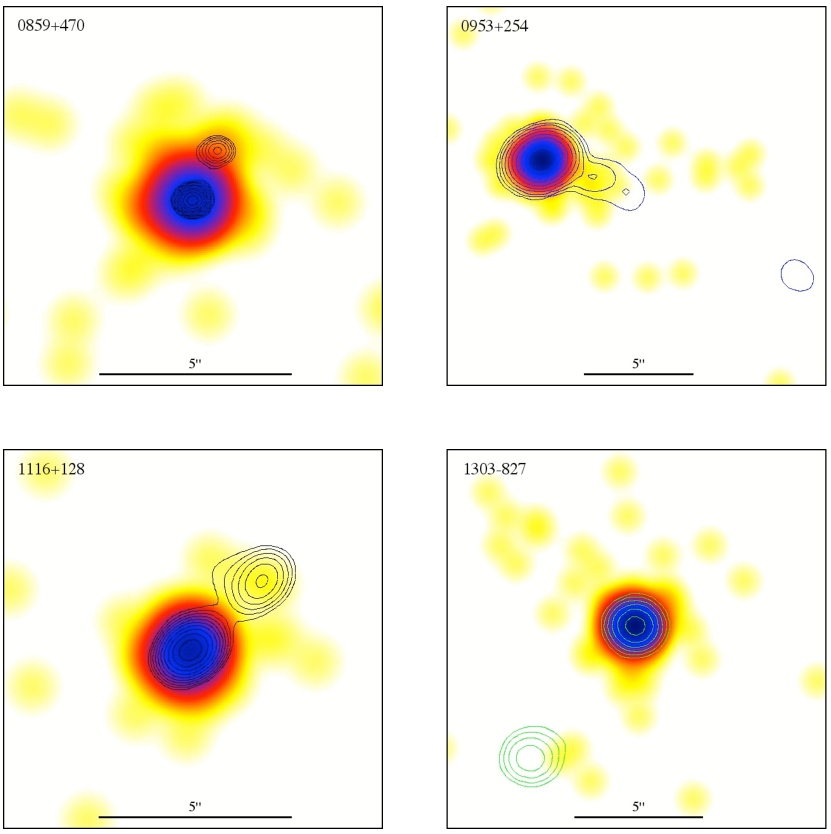
Figure 1: continued.

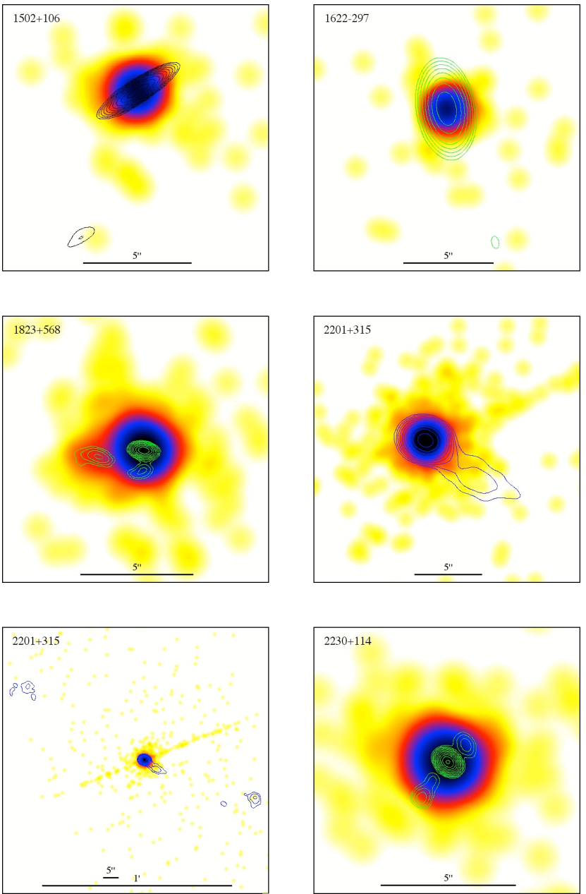
Figure 1: continued.

3.1 Core Spectral Fits

The X-ray spectrum of the nucleus for each source was measured using the CIAO v4.7 software (Fruscione et al., 2006) and CALDB 4.6.5 calibration database. On-source counts were extracted from a circle of radius $1.25^{\prime\prime}$ with local background sampled from a source-centered annulus, using a pie slice to exclude resolved X-ray jet emission where detected. Spectral data between 0.4 and 7 keV were binned to a minimum of 25 counts per bin and were fitted using the $\chi^{2}$ statistic in XSPEC (Arnaud, 1996), initially to a power-law model of fixed Galactic absorption. If the fit was good (the majority of cases) no additional components were added. If not, intrinsic absorption or a thermal component was added to the model to find an improved fit, and in some cases a pileup model was required. The results are given in Table 3, where the notes to the table or an entry in the $N_{\rm H_{\rm int}}$ column identify cases where a model more complex than a power law with Galactic absorption was used. The power-law slope, $\Gamma_{\rm x}$, is the photon spectral index, and so is $\alpha+1$ where $\alpha$ is the energy spectral index more commonly used in radio astronomy ($S\propto\nu^{-\alpha}$).

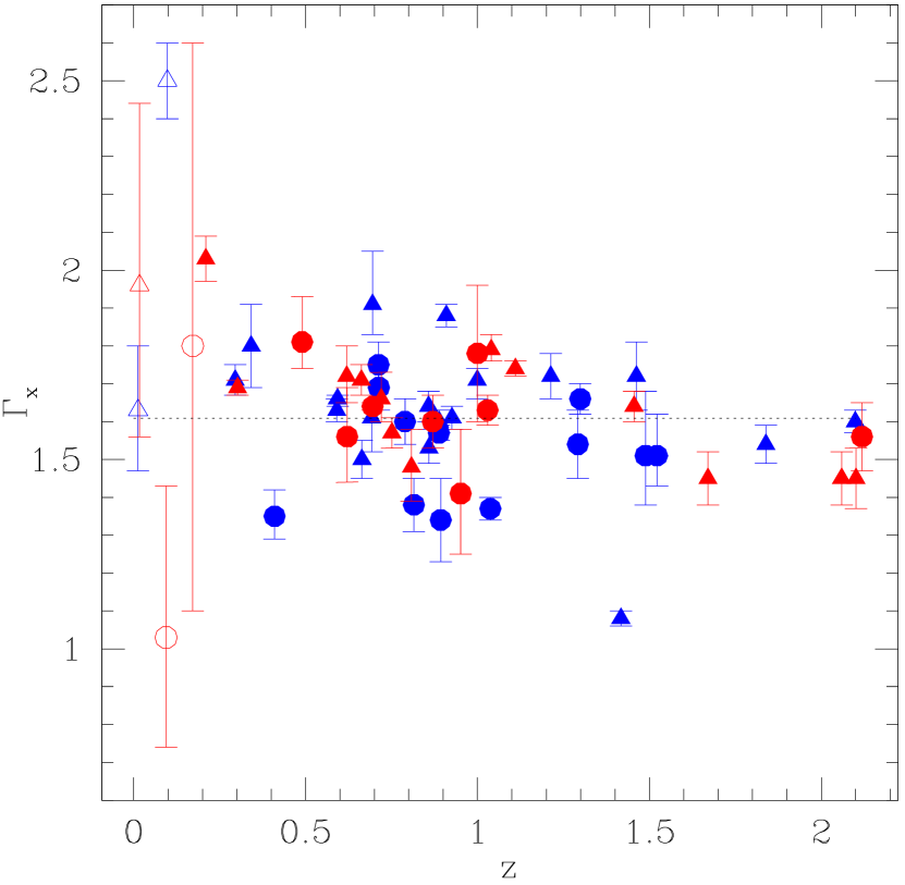
Figure 2: X-ray spectral indices of the cores plotted against redshift. Objects with X-ray jet emission (this paper) are shown as triangles, and those without as circles. Unfilled symbols mark the five objects at $z<0.2$ that are excluded from the calculation of the central value of the distribution (dotted line). The 32 sources that appear as $\gamma$-ray detections in the Fermi LAT 3LAC catalog (Ackermann et al., 2015) are shown in blue; the other 24 in red.

The X-ray spectral indices are plotted against redshift in Figure 2. We follow practice dating from the Einstein Observatory of assuming that the underlying spectral-index distribution has a normal distribution, and maximize the likelihood to find the best-fit underlying mean and dispersion (Maccacaro et al., 1988; Worrall, 1989). For the 51 objects at $z>0.2$, with 90% joint-confidence uncertainties, we find $\bar{\Gamma}_{\rm x}=1.61\pm 0.05$ and $\sigma=0.15^{+0.04}_{-0.03}$. These uncertainties are improved with respect to Paper I, and further confirm the flatter spectral index found in radio-loud quasars as compared with radio-quiet quasars for which $\bar{\Gamma}_{\rm x}\approx 1.9$ (Reeves & Turner, 2000). Our results are consistent with Belsole et al. (2006) who, from studying the X-ray spectra of radio-loud quasars and radio galaxies matched in extended radio power, conclude that the X-ray emission of core-dominated quasars is dominated by a beamed inverse-Compton jet component that is flatter in spectrum than other emission. The model of a radio-loud quasar’s X-ray spectrum being comprised of both isotropic and a beamed jet component was first proposed based on Einstein data due to a larger X-ray to radio flux ratio with increasing core dominance (Worrall et al., 1987), and the model is supported by more recent flux comparisons for larger samples (Miller et al., 2011).

Figure 2 hints at decreased $\Gamma_{\rm x}$ and $\sigma$ at high redshift: the seven objects above $z=1.5$ (five of which have X-ray jets) give $\bar{\Gamma}_{\rm x}=1.53^{+0.06}_{-0.08}$ and $\sigma=0.04^{+0.08}_{-0.04}$. Figure 3 compares 90% joint confidence contours in spectral index and dispersion for the 7 quasars at $z>1.5$ and the 44 at $0.2<z<1.5$. The plot implies that the probability that the two subsamples are drawn from the same parent distribution is $<1\%$. The two caveats to this result are that the choice of a dividing redshift of 1.5 is guided by the observations, and the dependence of luminosity with redshift in the sample means that any tendency towards flatter spectral index and a tighter distribution may be more associated with higher luminosity than higher redshift. Figure 4 shows the dependence of luminosity with redshift in the radio (with core and extended jet emission shown separately) and the X-ray. The trend is most obvious in the core radio, as expected from the flux-density thresholds applied during sample selection, but can also be seen in the X-ray and, with somewhat larger scatter, in the extended radio emission. Figures 2 and 4 both differentiate by color the sources that show as Fermi $\gamma$-ray detections in the LAT 3LAC catalog (Ackermann et al., 2015), and by symbol the sources with extended X-ray jet emission as found in this paper. It is noticeable that the Fermi detections (57%) are distributed across the redshift, luminosity, and X-ray spectral-index range of our sources rather than being clustered in any particular range. There is also no obvious association between the detection of $\gamma$-rays and resolved X-ray jets. Radio-loud quasars detected in $\gamma$-rays have been found to participate with BL Lac objects in what has been termed the ‘blazar sequence’, whereby the spectral energy distributions (SEDs) spanning radio and $\gamma$-ray are ‘bluer’ as bolometric luminosity increases (Fossati et al., 1998). As with the luminosities shown in Figure 4, blazar-sequence bolometric luminosities are calculated assuming that the emission is isotropic, and the sequence is modelled as a growth of the inverse-Compton relative to lower-energy synchrotron hump in the SED, such that $\gamma$-ray emission dominates the luminosity for powers above about $10^{38}$ W. While a physical understanding of the blazar sequence and the extent to which selection effects contribute remain matters for debate (see e.g., Giommi et al., 2012), Ghisellini et al. (2017) have argued empirically from the average SEDs of radio-loud quasars in the $\gamma$-ray-selected 3LAC catalog that observed X-ray spectral index becomes flatter with increasing isotropic bolometric luminosity. In time, more of the sources in our radio-selected sample may gather Fermi detections, and allow core X-ray spectral index to be looked at in a statistically more meaningful way in the context of radio to $\gamma$-ray SED, luminosity, redshift, extended-jet characteristics, and beaming parameters.

Table 3: Quasar X-ray Core Parameters

B1950	z	OBSID	Count Rate	Streak Rate	$N_{\rm H_{\rm Gal}}$	$\Gamma_{\rm x}$	$N_{\rm H_{\rm int}}$	$S_{\rm x}$	$\chi^{2}/$(dof)
			(cps)	(cps)	($10^{21}$ cm-2)		($10^{22}$ cm-2)	(nJy)
$0106+013$	2.099	10380,10799	$0.108\pm 0.004$	$0.09\pm 0.06$	0.280	$1.60\pm 0.03$	$\cdots$	$154\pm 4$	330.8/300
$0144-522$	0.098	10366	$0.089\pm 0.004$	$0.07\pm 0.07$	0.339	$2.5\pm 0.1$	$\cdots$	$94\pm 4$	7.2/16
$0208-512$	0.999	4813	0.305 $\pm$ 0.008	0.54 $\pm$ 0.15	0.294	$1.71^{+0.03}_{-0.05}$	$\cdots$	$245\pm 4$	236.6/206
$0229+131$	2.059	3109	0.111 $\pm$ 0.005	0.08 $\pm$ 0.10	0.83	$1.45\pm 0.07$	$\cdots$	106 $\pm$ 6	19.3/24
$0234+285$	1.213	4898	$0.283\pm 0.007$	$0.30\pm 0.09$	0.842	$1.72\pm 0.06$	$0.5\pm 0.1$	$317_{-16}^{+17}$	60.6/73
$0256+075$	0.893	10375	$0.155\pm 0.005$	$0.10\pm 0.07$	1.147	$1.34\pm 0.11$	$\cdots$	$130_{-16}^{+18}$	30.6/28
$0402-362$	1.417	10374	$1.337\pm 0.016$	$1.40\pm 0.23$	0.080	$1.08\pm 0.02$	$\cdots$	$857\pm 14$	196.9/196
$0413-210$	0.808	3110	0.063 $\pm$ 0.004	0.09 $\pm$ 0.11	0.239	$1.48^{+0.10}_{-0.09}$	$\cdots$	$57\pm 4$	6.3/11
$0454-463$	0.858	4893	$0.361\pm 0.008$	$0.46\pm 0.13$	0.235	$1.64\pm 0.04$	$\cdots$	$327\pm 9$	85.5/64
$0508-220$	0.172	10367	$0.010\pm 0.001$	$-0.01\pm 0.04$	0.257	$1.8^{+0.8}_{-0.7}$	$\cdots$	$10^{+6}_{-4}$	0.7/1
$0707+476$	1.292	10368	$0.103\pm 0.004$	$0.11\pm 0.07$	0.806	$1.54\pm 0.09$	$\cdots$	$90\pm 6$	22.1/17
$0745+241$	0.410	3111	0.160 $\pm$ 0.006	0.23 $\pm$ 0.16	0.516	$1.35^{+0.07}_{-0.06}$	$\cdots$	$131^{+7}_{-6}$	23.5/22
$0748+126$	0.889	10376	$0.449\pm 0.009$	$0.34\pm 0.12$	0.360	$1.60\pm 0.03$	$\cdots$	$385\pm 9$	61.9/76
$0820+225$	0.951	4897	$0.034\pm 0.003$	$0.11\pm 0.07$	0.390	$1.41^{+0.17}_{-0.16}$	$\cdots$	$27\pm 3$	4.8/4
$0833+585$	2.101	7870	$0.160\pm 0.007$	$0.01\pm 0.05$	0.443	$1.45\pm 0.08$	$\cdots$	$122\pm 7$	31.5/19
$0858-771$	0.490	3112	0.130 $\pm$ 0.005	0.52 $\pm$ 0.21	1.021	$1.81^{+0.12}_{-0.07}$	$\cdots$	$145^{+15}_{-7}$	18.1/17
$0859+470$	1.462	10371	$0.075\pm 0.004$	$0.01\pm 0.04$	0.192	$1.72\pm 0.09$	$\cdots$	$63\pm 4$	12.1/14
$0903-573$	0.695	3113	0.123 $\pm$ 0.005	0.00 $\pm$ 0.08	3.212	$1.91^{+0.14}_{-0.08}$	$\cdots$	$199^{+26}_{-12}$	14.9/16
$0920-397$	0.591	5732,7220-1,7223	0.105 $\pm$ 0.005	0.11 $\pm$ 0.12	2.147	1.63 $\pm$ 0.03	$\cdots$	$149^{+3}_{-9}$	173.4/174
$0923+392$	0.695	3048	$0.655\pm 0.006$	$0.84\pm 0.10$	0.143	$1.64\pm 0.01$	$\cdots$	$514\pm 5$	207.3/209
$0953+254$	0.712	10377	$0.134\pm 0.005$	$0.06\pm 0.06$	0.267	$1.75\pm 0.06$	$\cdots$	$121\pm 5$	15.9/26
$0954+556$	0.909	4842	$0.109\pm 0.002$	$0.10\pm 0.03$	0.089	$1.88\pm 0.03$	$\cdots$	$91\pm 2$	110.5/112
$1030-357$	1.455	5730	0.069 $\pm$ 0.004	0.14 $\pm$ 0.14	0.609	$1.64\pm 0.04$	$\cdots$	$52\pm 2$	57.8/52
$1040+123$	1.029	2136	$0.178\pm 0.004$	$0.09\pm 0.05$	0.287	$1.63\pm 0.04$	$\cdots$	$139\pm 3$	58.0/62
$1046-409$	0.620	3116	0.196 $\pm$ 0.007	-0.01 $\pm$ 0.09	0.829	$1.72^{+0.08}_{-0.07}$	$\cdots$	$202^{+11}_{-9}$	16.4/23
$1055+018$	0.888	2137	$0.594\pm 0.008$	$0.58\pm 0.13$	0.396	$1.57\pm 0.02$	$\cdots$	$442\pm 6$	143.5/149
$1055+201$	1.110	5733	$0.214\pm 0.007$	$0.12\pm 0.08$	0.182	$1.74\pm 0.02$	$\cdots$	$247\pm 3$	163.3/176
$1116+128$	2.118	10373	$0.083\pm 0.004$	$0.10\pm 0.07$	0.240	$1.56\pm 0.09$	$\cdots$	$70\pm 4$	15.0/15
$1116-462$	0.713	4891	$0.207\pm 0.006$	$0.32\pm 0.11$	1.040	$1.69\pm 0.06$	$\cdots$	$210\pm 8$	27.6/39
$1145-676$	0.210	3117	0.292 $\pm$ 0.008	0.49 $\pm$ 0.23	3.189	2.03 $\pm$ 0.06	$\cdots$	$540\pm 25$	119.3/111
$1202-262$	0.789	3118	0.147 $\pm$ 0.005	0.16 $\pm$ 0.13	0.708	1.60 $\pm$ 0.06	$\cdots$	$137\pm 6$	19.5/26
$1251-713$	$\cdots$	4892	$0.043\pm 0.003$	$-0.04\pm 0.03$	2.119	$1.78\pm 0.18$	$\cdots$	$53\pm 6$	6.6/6
$1258-321$	0.01704	3119	0.011 $\pm$ 0.002	0.09 $\pm$ 0.16	0.575	$1.96^{+0.48}_{-0.40}$	$\cdots$	$14^{+6}_{-3}$	6.5/2
$1303-827$	0.870	10365	$0.132\pm 0.005$	$0.06\pm 0.06$	0.720	$1.60\pm 0.07$	$\cdots$	$122\pm 5$	16.0/24
$1343-601$	0.01292	3120	0.252 $\pm$ 0.007	0.53 $\pm$ 0.27	10.6	$1.63^{+0.17}_{-0.16}$	1.08 $\pm$ 0.24	$870^{+240}_{-180}$	35.1/35
$1354+195$	0.720	2140	$0.583\pm 0.008$	$0.93\pm 0.15$	0.223	$1.66^{+0.07}_{-0.06}$	$\cdots$	$519\pm 23$	165.1/142
$1421-490$	0.662	5729	$0.049\pm 0.003$	$0.07\pm 0.06$	1.457	$1.71\pm 0.04$	$\cdots$	$47\pm 2$	72.0/62
$1424-418$	1.522	3121	0.189 $\pm$ 0.007	0.08 $\pm$ 0.12	0.805	$1.51^{+0.11}_{-0.08}$	$\cdots$	$181^{+20}_{-11}$	13.8/23
$1502+106$	1.839	10378	$0.204\pm 0.006$	$0.19\pm 0.09$	0.237	$1.54\pm 0.05$	$\cdots$	$167\pm 6$	39.2/39
$1622-297$	0.815	10370	$0.149\pm 0.005$	$0.09\pm 0.07$	1.528	$1.38\pm 0.07$	$\cdots$	$138\pm 8$	22.7/27
$1641+399$	0.5928	10379	$0.625\pm 0.008$	$1.14\pm 0.16$	0.104	$1.66_{-0.02}^{+0.01}$	$\cdots$	$489\pm 5$	238.6/245
$1642+690$	0.751	2142	$0.154\pm 0.004$	$0.12\pm 0.06$	0.434	$1.57\pm 0.04$	$\cdots$	$119\pm 4$	38.7/42
$1655+077$	0.621	3122	0.165 $\pm$ 0.006	0.09 $\pm$ 0.14	0.626	$1.56^{+0.13}_{-0.12}$	$\cdots$	$153^{+21}_{-16}$	38.3/22
$1655-776$	0.0947	3123	0.031 $\pm$ 0.003	0.02 $\pm$ 0.11	0.830	$1.03^{+0.40}_{-0.29}$	$\cdots$	$41^{+23}_{-9}$	4.2/2
$1823+568$	0.664	10369	$0.516\pm 0.010$	$0.64\pm 0.16$	0.411	$1.50\pm 0.05$	$0.16\pm 0.05$	$449\pm 20$	81.6/84
$1828+487$	0.692	3124	0.421 $\pm$ 0.009	0.73 $\pm$ 0.25	0.66	1.61 $\pm$ 0.09	$\cdots$	344 $\pm$ 10	74.6/61
$1928+738$	0.302	2145	$0.781\pm 0.010$	$1.08\pm 0.16$	0.800	$1.69\pm 0.02$	$\cdots$	$705\pm 10$	195.2/162
$2007+777$	0.342	5709	$0.226\pm 0.003$	$0.29\pm 0.11$	0.879	$1.80\pm 0.11$	$0.13\pm 0.03$	$1460\pm 200$	177.1/189
$2052-474$	1.489	3125	0.113 $\pm$ 0.005	0.48 $\pm$ 0.21	0.404	$1.51^{+0.17}_{-0.13}$	$\cdots$	$109^{+18}_{-10}$	10.3/15
$2101-490$	1.040	5731	0.060 $\pm$ 0.003	0.07 $\pm$ 0.11	0.341	$1.79^{+0.04}_{-0.03}$	$\cdots$	$84^{+3}_{-2}$	90.0/106
$2123-463$	1.67	4890	$0.098\pm 0.004$	$0.07\pm 0.06$	0.330	$1.45\pm 0.07$	$\cdots$	$80\pm 4$	19.9/21
$2201+315$	0.295	9283	$0.580\pm 0.008$	$0.75\pm 0.13$	1.170	$1.71\pm 0.04$	$\cdots$	$586\pm 16$	135.7/141
$2230+114$	1.037	10372	$0.473\pm 0.009$	$0.23\pm 0.10$	0.499	$1.37\pm 0.03$	$\cdots$	$374\pm 76$	76.5/79
$2251+158$	0.859	3127	0.656 $\pm$ 0.012	2.89 $\pm$ 0.50	0.713	$1.53^{+0.05}_{-0.04}$	$\cdots$	$1225^{+270}_{-170}$	126.6/121
$2255-282$	0.926	4894	$0.383\pm 0.007$	$0.18\pm 0.08$	0.228	$1.61\pm 0.03$	$\cdots$	$328\pm 7$	88.7/82
$2326-477$	1.299	4896	$0.199\pm 0.005$	$0.15\pm 0.07$	0.169	$1.66\pm 0.04$	$\cdots$	$174\pm 5$	46.3/54

Note. — Count rates and streak rates are for the OBSIDs used for the extended analysis. Core spectra use deeper exposures where available. Errors in spectral parameters are $1\sigma$.

Figure 3: 90% confidence contours (4.61 above the minimum value of $-2\ln$ likelihood) for the two interesting parameters of mean spectral index and intrinsic dispersion. The comparison between the 7 quasars at $z>1.5$ and the 44 at $0.2<z<1.5$ finds less than 1% probability that they are drawn from the same parent distribution.

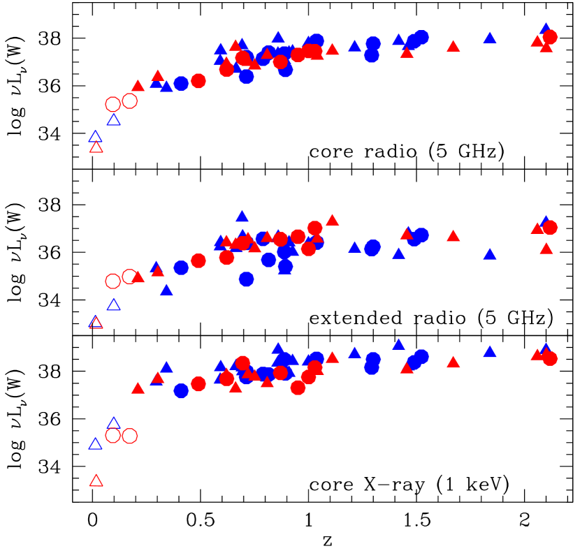
Figure 4: Rest-frame isotropic luminosities (disregarding beaming) against redshift for emissions in 5-GHz core radio (top), 5-GHz extended radio (middle) and 1-keV X-ray (bottom), showing the extent to which luminosity and redshift are related in our sample. Colors and symbols are as in Figure 2.

3.2 Imaging results

We tested for the detection of X-rays from a jet using a simple Poisson test, as in Paper I, for counts in a rectangular region of appropriate width extending over a specific angular range ($\theta_{i}$, $\theta_{o}$) from the core at a specific position angle. The radio images were used to define the position angles and lengths of possible jets. Most jets are clearly defined as one-sided structures but in a few ambiguous cases the pc-scale images were used to define the jet direction, when available. The parameters of the selection regions are given in Table 4. The width of the rectangle was 3″ except for 0144$-$522, 0505$-$220, 0748$+$126, 0953$+$254, 1116$+$128, and 2201$+$315, where the jets bend substantially, so the rectangles were widened to 4-8″. Profiles of the radio emission along the jets are shown in Fig. 5. In order to eliminate X-ray counts from the wings of the quasar core, a profile was computed at 90° to the jet and subtracted giving the net counts, $C_{\rm net}$, in Table 4. Except for Q0106$+$013, there was insufficient signal to provide interesting limits on the X-ray spectral indices of the jet without contamination by the much brighter quasar core. CIAO was used to extract the jet spectrum of Q0106$+$013, which was fit to a power law (as used for quasar core fitting in §3.1) using isis, giving $\Gamma_{\rm x}=1.60^{+0.46}_{-0.27}$ and negligible $N_{\rm H}$. The X-ray counts in the same rectangular region defined by the radio data were compared to a similar sized region on the opposite side of the core for the Poisson test. We set the critical probability for detection of an X-ray jet to 0.0025, which yields a 5% chance that there might be one false detection in a set of 20 sources. Histograms of the X-ray emission along the jets are shown in Fig. 5. The jet and counter-jet position angles are compared, providing a qualitative view of the X-ray emission along the jets. No counter-jets are apparent in the X-ray images.

Table 4: Quasar Jet X-ray Measurements

Target	PA	$\theta_{i}$	$\theta_{o}$	$S_{r}$	$\nu_{r}$	$C_{\rm net}$	Count Rate	$S_{x}$	$\alpha_{rx}$	$P_{jet}$	X?
	(°)	(″)	(″)	(mJy)	(GHz)		(10-3 cps)	(nJy)
0106$+$013	-175	1.5	6.0	487.8 $\pm$ 2.7	1.42	87	9.90 $\pm$ 1.11	9.9	0.94 $\pm$ 0.01	1.00e-10	Y
0144$-$522	100	1.5	20.0	15.7 $\pm$ 1.6	17.73	12	2.15 $\pm$ 0.91	2.1	0.96 $\pm$ 0.03	1.30e-04	Y
0256$+$075	100	1.5	6.0	5.8 $\pm$ 1.7	1.42	2	0.36 $\pm$ 0.50	$<$ 1.9	$>$ 0.79	1.85e-01	N
0402$-$362	170	1.5	14.0	47.4 $\pm$ 1.6	8.64	22	4.12 $\pm$ 2.23	4.1	0.95 $\pm$ 0.03	2.32e-03	Y
0508$-$220	150	1.5	25.0	516.3 $\pm$15.5	1.42	-5	-0.94 $\pm$ 0.78	$<$ 1.4	$>$ 1.04	9.62e-01	N
0707$+$476	85	1.5	6.0	12.7 $\pm$ 2.5	4.86	-2	-0.38 $\pm$ 0.46	$<$ 1.0	$>$ 0.92	9.08e-01	N
0748$+$126	130	1.5	15.0	14.5 $\pm$ 2.1	4.86	22	3.92 $\pm$ 1.55	3.9	0.85 $\pm$ 0.02	8.98e-05	Y
0833$+$585	90	1.5	5.0	9.0 $\pm$ 1.4	1.42	17	4.51 $\pm$ 1.27	4.5	0.77 $\pm$ 0.02	1.00e-10	Y
0859$+$470	-20	1.0	4.0	114.0 $\pm$ 4.1	4.86	10	1.78 $\pm$ 0.76	1.8	1.01 $\pm$ 0.02	7.63e-05	Y
0953$+$254	-115	1.5	15.0	30.3 $\pm$ 2.3	1.42	4	0.71 $\pm$ 0.71	$<$ 2.9	$>$ 0.85	8.39e-02	N
1116$+$128	-45	1.5	10.0	101.6 $\pm$ 2.8	4.86	2	0.36 $\pm$ 0.57	$<$ 2.1	$>$ 1.00	2.15e-01	N
1303$-$827	140	1.5	8.0	77.2 $\pm$ 3.2	8.64	2	0.36 $\pm$ 0.56	$<$ 2.0	$>$ 1.02	2.15e-01	N
1502$+$106	160	1.5	9.0	6.4 $\pm$ 2.4	4.86	6	1.25 $\pm$ 0.69	1.2	0.87 $\pm$ 0.04	2.84e-03	Y
1622$-$297	-160	1.5	10.0	69.9 $\pm$ 5.6	8.64	4	0.71 $\pm$ 0.71	$<$ 2.9	$>$ 0.99	8.39e-02	N
1823$+$568	90	1.0	4.0	113.5 $\pm$ 6.2	4.86	60	10.75 $\pm$ 2.20	10.8	0.91 $\pm$ 0.01	1.00e-10	Y
2201$+$315	-110	1.5	40.0	158.1 $\pm$ 5.1	1.42	27	2.95 $\pm$ 1.35	2.9	0.94 $\pm$ 0.02	3.35e-04	Y
2230$+$114	140	1.0	4.0	86.2 $\pm$ 6.4	4.86	6	1.28 $\pm$ 1.63	$<$ 6.2	$>$ 0.82	1.40e-01	N

Note. — The jet radio flux density is measured at $\nu_{r}$ for the same region as for the X-ray count rate, given by the PA, $\theta_{i}$, and $\theta_{o}$ values. The X-ray flux density is given at 1 keV assuming a conversion of 1 $\mu$Jy/(count/s), which is good to $\sim$ 10% for power law spectra with low column densities and X-ray spectral indices near 0.5.

Figure 5: Profiles of the radio emission (left) and X-ray counts from Chandra (right) along the jet. The position angles of the jets are defined in Table 4. The vertical dashed lines demarcate the jet regions. Dotted lines in the radio panels give the profiles at a position angle 90° clockwise from the jet to avoid counter-jets. The bold, solid lines (left) give the differences between the profiles along the jet and perpendicular to it, nulling the core effectively. The horizontal dash-dot lines (left) are set to the average noise levels in each radio map. Because there are no clearly detected counter-jets in the X-ray images, dotted lines (right) give the profiles at a position angle 180° clockwise from the jet.

Figure 5: continued.

Figure 5: continued.

Figure 5: continued.

Figure 5: continued.

Figure 5: continued.

Jet X-ray flux densities (Table 4) were computed from count rates using the conversion factor 1 count/s $=$ 1 $\mu$Jy. This conversion is accurate to within 10% for typical power law spectra. The spectral index from radio to X-ray is computed using $\alpha_{rx}=-\log(S_{x}/S_{r})/\log(\nu_{x}/\nu_{r})$, where $\nu_{x}=2.42\times 10^{17}$ Hz and $\nu_{r}$ depends on the map used.

Table 5: Hubble Space Telescope Observations

Target	HST ID	Exposure (s)	Date
0144$-$522	ib9402	2845.4	2010-04-12
0256$+$075	ib9412	2545.4	2010-01-13
0402$-$362	ib9411	2695.4	2010-07-16
0508$-$220	ib9403	2695.4	2010-07-18
0707$+$476	ib9405	2695.4	2009-10-04
0748$+$126	ib9415	2545.4	2009-10-12
0859$+$470	ib9408	2695.4	2009-10-01
0953$+$254	ib9413	2695.4	2010-11-21
1116$+$128	ib9410	2545.4	2010-02-21
1303$-$827	ib9404	2995.4	2010-05-18
1502$+$106	ib9414	2545.4	2010-03-14
1622$-$297	ib9406	2695.4	2010-05-08
1823$+$568	ib9407	2845.4	2009-10-12
2230$+$114	ib9409	2545.4	2009-10-12

Table 6: IR Knot Fluxes

Target	$S_{\rm BG,noise}$	$S_{\rm knot}$	$\alpha_{ri}$
	($\mu$Jy)	($\mu$Jy)
0144$-$522	0.515	1.744 $\pm$ 0.865	$>$ 0.66
0256$+$075	0.022	-0.053 $\pm$ 0.032	$>$ 0.92
0402$-$362	0.015	8.334 $\pm$ 0.535	$>$ 0.72
0508$-$220	0.014	-0.166 $\pm$ 0.025	$>$ 1.16
0707$+$476	1.121	0.679 $\pm$ 1.858	$>$ 0.67
0748$+$126	0.338	-1.260 $\pm$ 0.463	$>$ 0.76
0859$+$470	0.225	0.032 $\pm$ 0.281	$>$ 1.10
0953$+$254	0.046	-0.066 $\pm$ 0.081	$>$ 0.87
1116$+$128	0.031	-0.322 $\pm$ 0.056	$>$ 1.21
1303$-$827	0.013	0.017 $\pm$ 0.028	$>$ 1.33
1502$+$106	0.022	-0.069 $\pm$ 0.030	$>$ 0.92
1622$-$297	0.027	0.072 $\pm$ 0.048	$>$ 1.06
1823$+$568	0.379	-1.071 $\pm$ 0.577	$>$ 0.96
2230$+$114	0.167	-0.626 $\pm$ 0.249	$>$ 1.07

Note. — Jet knot flux densities were measured in 0.5$\arcsec$ radius circles centered at the peak of the radio emission, while the $1\sigma$ background noise fluxes are from locations with comparable confusion. Limits to the spectral index between the radio and IR bands is given as $\alpha_{ri}$. Confusion involves quasar and stellar diffraction spikes and foreground galaxies (as in the case of 0402$-$362). These values are meant to be indicative, primarily; more accurate measurements for two sources are given in Tables 8 and 7. See text for details.

3.3 Optical Jet Measurements

Images were obtained using the Hubble Space Telescope Wide Field Camera 3 (WFC3) IR channel and the F160W filter (Table 5). The drizzled images were examined using SAOImage ds9 v7.6; Fig. 6 shows the HST images overlaid with contours from the radio maps after registering images to the cores. Simple IR flux limits for point-like knots were determined using ds9 by placing a 0.$\arcsec$5 radius aperture at the location of the peak radio flux for each jet. Often, these positions suffered from some confusion with foreground sources, the host galaxy, or stellar diffraction spikes. In order to take such confusion into account to first order, a background aperture of the same size was placed in a comparable position relative to the source of confusion – e.g., on the opposite side of the galaxy or diffraction spike. The ds9 Analysis/Statistics tool reports the total electron rate, $r$ (in e${}^{-}{\rm s}^{-1}$), and the region’s variance per pixel, $V$, for $n$ pixels, where $n=48$ for the drizzled image scale of 0.1283$\arcsec$ per pixel. For $r_{b}$ in the background region, $r_{k}$ in the knot, and associated variances $V_{b}$ and $V_{k}$, the background noise is $(nV_{b})^{1/2}$, and the net source rate is $r_{k}-r_{b}$ $\pm$ $(nV_{b}+nV_{k})^{1/2}$. The result is scaled by $1.505\times 10^{-7}$ Jy s/e^-, the inverse sensitivity of the F160W filter (as found in the image header’s photfnu keyword). The fluxes are given in Table 6. Without confusion, the typical flux noise for point-like sources is about 0.014 $\mu$Jy, so a 3$\sigma$ flux limit would be about 0.05 $\mu$Jy at the so-called pivot wavelength of 1.537 $\mu$m, or $\nu=1.95\times 10^{14}$ Hz. Fluxes were corrected for enclosed energy by dividing by 0.854, based on the on-line WFC3 encircled energy table for 0.$\arcsec$5 radius apertures at a wavelength of 1.5 $\mu$m. Limits to the spectral index between the radio and IR bands is given as $\alpha_{ri}$, where $S_{r}=S_{\rm IR}\nu^{\alpha_{ri}}$. Limits to $S_{\rm IR}$ were set to $3\sigma_{\rm knot}$ plus the measured flux, if positive. In almost all cases, $\alpha_{ri}$ is greater than 0.8, a commonly observed spectral index in the radio band for jet knots, indicating that a synchrotron model would break between the radio and IR bands for these knots.

In two cases, 0144$-$522 and 0508$-$220, the host galaxies were sufficiently bright that it is difficult to see jet-related emission on the images. Purely elliptical models of each of these galaxies were created using the iraf ellipse tasks, after masking bright stars and galaxies that can distort the fits. The results from fitting these two observations are shown in Figs. 7 and 10. See the notes on individual sources for details.

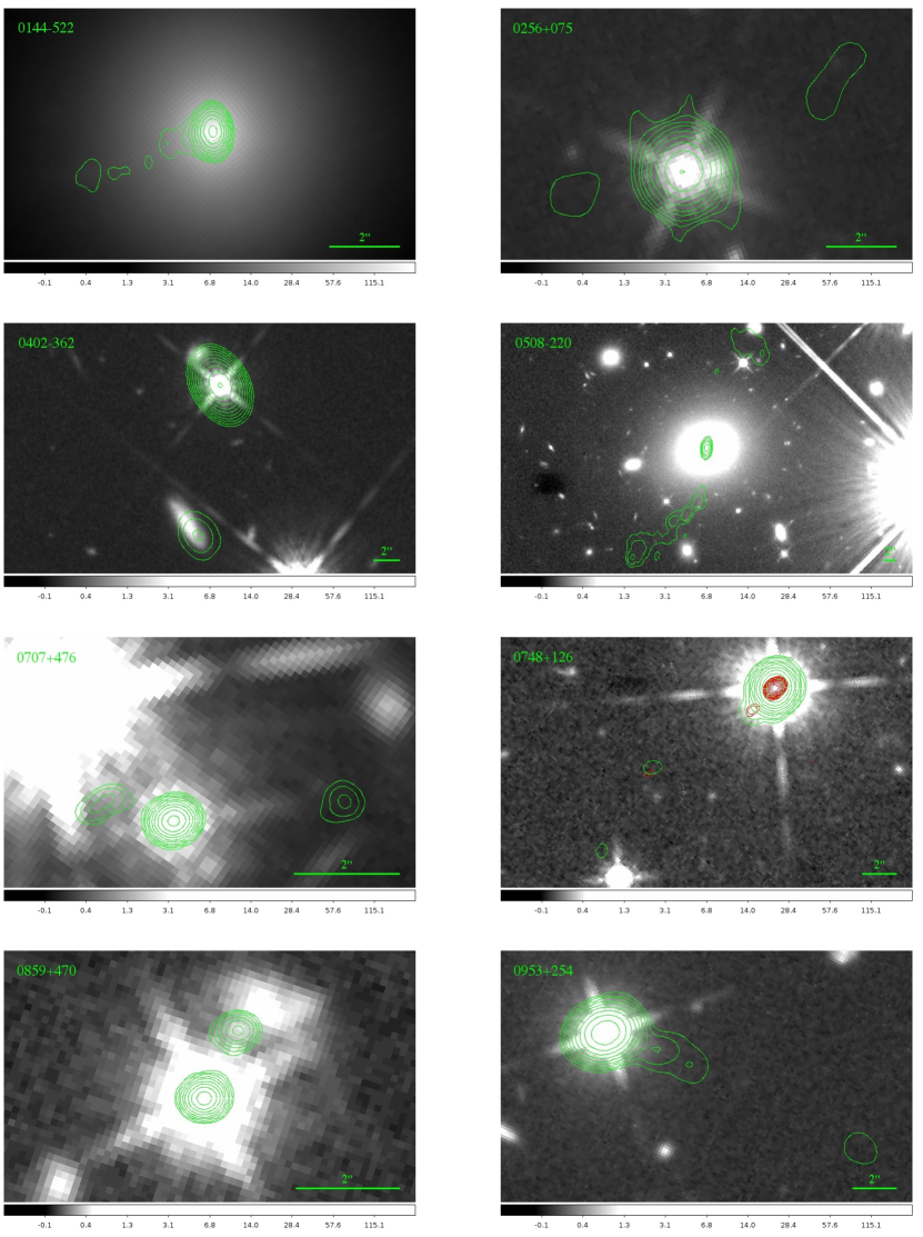
Figure 6: Overlays of radio contours on drizzled infrared images (grayscale) in the F160W filter with the HST Wide Field Camera 3. Radio contours are the same as in Fig. 1. Even without subtracting galaxy models or point source functions for the quasar cores, there are very few detections of kpc-scale jet emission. For 0144$-$522, the kpc-scale jet is observed within the profile of the bright host galaxy and in 0859$+$470, there is a possible feature associated with a knot about 1″ from the core to the northwest. Galaxy-subtracted images of 0144$-$522 and 0508$-$220 are shown in Fig. 7 and Fig. 10.

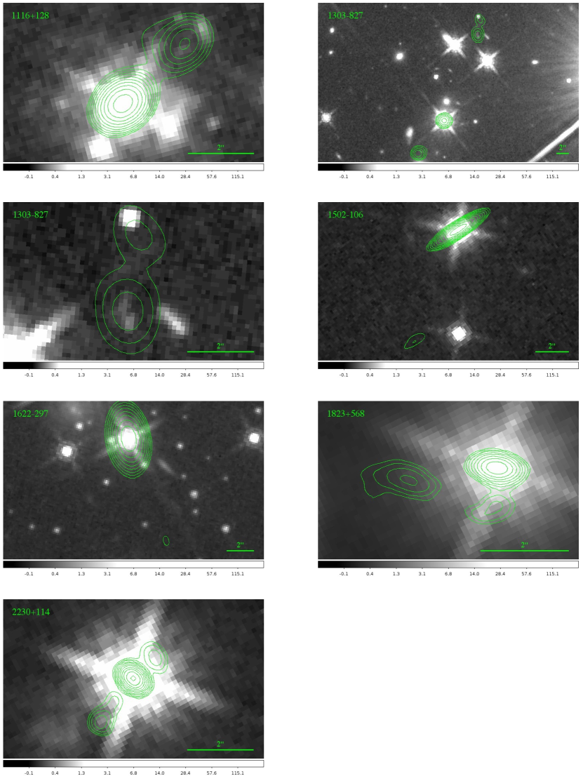
Figure 6: continued.

3.4 Notes on Individual Sources

In this section, we present qualitative descriptions of the X-ray and radio morphologies shown in Figure 1 and describe the directions of any pc scale jets. Profiles of the radio and X-ray emission along the jets are given in Figure 5. All position angles (PAs) are defined as positive when east of north with due north defining zero. Unless noted, VLBI imaging information comes from the MOJAVE project Lister et al. (2009a).

0106$+$013 (4C $+$01.02)

The X-ray image was first published by Hogan et al. (2011). The jet extends almost directly south for about 6″. The X-ray emission appears to end in the middle of the terminal hotspot, which peaks at about 4.5″ from the core. The quasar was not part of our observing program, so we do not have an HST image of it. VLBI mapping shows a jet at a PA of -120° with the greatest superluminal motion of the quasars in our sample: 24.4$c$.

0144$-$522 (PKS B0144$-$522)

The radio emission from the jet extends 20″ to the east, curving northeast while becoming significantly more diffuse and shows no hotspot, reminiscent of an FR I type morphology but one-sided. Simple galaxy modeling and subtraction (Fig. 7) was done with ellipse fitting in IRAF because the host galaxy is so bright in the HST image. There is a clear detection of the inner 3″ of the jet in both the X-ray and optical. The galaxy-subtracted HST data were analyzed separately using regions defined in Fig. 8, with background regions comparably placed with regard to the core’s diffraction spikes. Results are given in Table 7. The regions are not circular, so we applied an estimated aperture correction of 15% to the measured fluxes. Fig. 9 shows the spectral energy distribution (SED) that one obtains using the radio and X-ray fluxes from Table 4 and totaling the IR fluxes from Table 7. We find $\alpha_{ri}=0.76$ using these data, indicating that a single-population synchrotron model could explain the radio to IR SED. The X-ray flux is well below the extrapolation of the radio-IR spectrum, indicating that there must be a break in the spectrum, still consistent with a single-population synchrotron model.

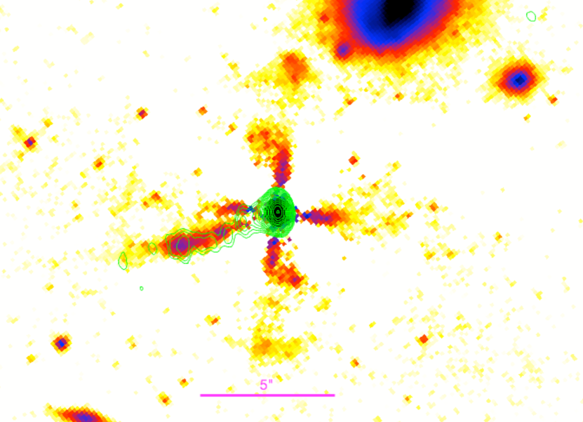
Figure 7: WFC3 image of 0144$-$522 after subtracting elliptical flux contours to eliminate the host galaxy light. No attempt was made to model the quasar core. The radio contours start at 0.3 mJy/beam and increase by a factor of $2^{1/2}$ per contour.

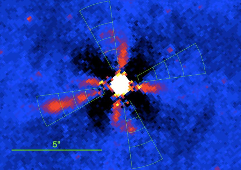
Figure 8: Same as Fig. 7 but with regions used for jet analysis (to east) and for background (to north, west, and south). Fluxes in the different annular arcs of the jet are given in Table 7.

Table 7: IR Measurements of 0144$-$522 Jet Regions

Region	$\theta_{i}$	$\theta_{o}$	$S_{\rm IR}$
	(″)	(″)	($\mu$Jy)
WK1.5	1.0	2.0	2.15 $\pm$ 0.38
WK2.35	2.0	2.7	2.03 $\pm$ 0.34
WK3.1	2.7	3.5	3.26 $\pm$ 0.34
WK4.1	3.5	4.7	6.22 $\pm$ 0.67

Note. — The jet optical flux densities were measured in the regions shown in Fig. 8, defined by $\theta_{i}$ and $\theta_{o}$, measured from the quasar core in an annular region between position angles 97$\arcdeg$ and 119$\arcdeg$ E of N.

Figure 9: Spectral energy distribution for the total jet in 0144$-$522. A single-population synchrotron model would require a break between the IR and X-ray bands.

0256$+$075 (PKS B0256$+$075)

The VLA image shows faint, small lobes to the northeast and due west. The latter is closer to the core and defines the region of interest for X-ray analysis. No X-ray emission was detected from the radio jet. The HST image shows what may be a knot about 1″ due west of the core but the radio map shows no clear extension in this direction.

0402$-$362 (PKS B0402$-$362)

The Chandra data show a marginally detected excess of flux in the box defined to include the southern radio hotspot. The HST image shows an edge-on spiral galaxy at the edge of the south hotspot, so the detection listed in Table 6 is likely to be a vast overestimate of any IR flux from the hotspot.

0508$-$220 (PKS B0508$-$220)

The primary radio structure starts about 5″ south of the core and curves to the east, ending 25″ from the core. A lobe is found to the northwest extending about as far as the southern lobe. The Chandra data do not show a significant detection. There is a rather bright elliptical galaxy at the location of the core in the HST image so elliptical contours were fit in a manner similar to that for 0144$-$522. The result of the galaxy subtraction is shown in Fig. 10. There are two faint sources near radio knots about 10$\arcsec$ to the south of the core. The fluxes of these possible knots and their positions were measured from the HST image using ds9 and results are given in Table 8. It is not clear if these sources are related to the radio-emitting knots.

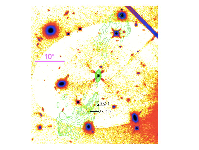
Figure 10: WFC3 image of 0508$-$220 after subtracting elliptical flux contours to eliminate the host galaxy light. No attempt was made to model the quasar core. A bright star to the SW biases the contour fits, causing over-subtraction of the galaxy in part of the jet region. The radio contours start at 5 mJy/beam and increase by a factor of $2^{1/2}$ per contour.

Table 8: IR Measurements of Possible 0508$-$220 Jet Knots

Knot	$\alpha$	$\delta$	$\theta$	$S_{\rm IR}$
	(°)	(°)	(″)	($\mu$Jy)
SK9.5	77.75249	-22.03465	9.49	1.052 $\pm$ 0.135
SK11.9	77.75310	-22.03522	11.93	0.949 $\pm$ 0.069

Note. — The jet optical flux densities were measured in 0.5$\arcsec$ radius circles centered at the given coordinates ($\alpha$, $\delta$), at distances $\theta$ from the core.

0707$+$476 (B3 0707$+$476)

There are weak knots to the east and west of the core, with the west one being slightly farther at about 3″ from the core. The jet continues beyond the east knot about 6″ (apparent in the radio profile), so we somewhat arbitrarily define the jet direction to be toward the east. VLBI imaging shows a pc scale jet to the northeast (Kellermann et al., 2004) but the apparent velocities given by Kellermann et al. (2004) are negative (but marginally significant) so we quote the absolute value and assume that the core location is not precisely known. The core lies quite close to a bright star in the HST image, avoiding its southern diffraction spike but the bright eastern knot lies practically on top of the spike so no jet features are apparent in the HST image.

0748$+$126 (PKS B0748$+$126)

The source has a straight radio jet to the southeast ending at a hotspot 15″ from the core. The PA of the VLBI jet is only 15° from that of the kpc scale jet and superluminal motion at just under 20$c$ was found. The jet and hotspot are both clearly detected in the 5.6 ks observation. No features are apparent in the HST image at any of the radio jet knots.

0833$+$585 (SBS 0833$+$585)

The radio jet starts out to the east but goes through an apparent bend at a right angle about 4″ from the core. The section before the bend is clearly detected in X-rays and there is a marginal detection also of the hotspot at the end, about 10″ to the southwest.

0859$+$470 (4C $+$47.29)

The extended radio emission consists of a single knot at 3″ northwest of the core, detected by Chandra. There is an extended feature slightly farther out from the core in the HST image and there appears to be optical emission associated with the knot.

0953$+$254 (B2 0954$+$25A)

The radio jet starts out at a PA of -115°, as in VLBI images, and wiggles a few times before ending at a hotspot 15″ from the core. No corresponding features are detected in the X-ray band. Similarly, there are no clear knot associations in the HST image.

1116$+$128 (4C $+$12.39)

The extended radio emission consists of a single knot at 2.5″ northwest of the core. The knot is not detected in the Chandra data. No features are apparent in the HST image at the radio knot.

1303$-$827 (PKS 1302$-$82)

The extended radio emission consists of a single knot at 6.5″ southeast of the core and a knot pair about 16″ north-northwest of the core. The X-ray jet searched was set to the SE to include the closest knot. No knots are detected by Chandra. In the HST image, there is faint, resolved flux from the closer of the NNW knot pair, shown in a inset in Fig. 6.

1502$+$106 (B2 0954$+$25A)

The VLBI jet is oriented at a PA of 120°, while the kpc scale jet is at a PA of 160° (see Table 10) and is marginally detected. The VLA image of the jet published by Cooper et al. (2007) shows a continuous jet all the way to the termination, about 9″ from the core. Lister et al. (2013) found a maximum apparent speed of VLBI knots of 17.5$c$. The HST image shows no clear detection of any part of the kpc scale jet.

1622$-$297 (PKS B1622$-$297)

The kpc radio jet is weak and not detected with Chandra. There is a pc-scale jet at a PA of -70°with maximum apparent speed of 18.6$c$ (Lister et al., 2013). There are no apparent features in the HST image that are associated with radio or X-ray emission.

1823$+$568 (4C $+$56.27)

There is a pc-scale jet at a PA of -160° with maximum apparent speed of 26.17 $c$ (Lister et al., 2013). The kpc scale jet is first oriented almost due south but bends about 1″ from the core to the east, where it is clearly detected in the Chandra image at 2.5″ from the core. There are no apparent features in the HST image that are associated with radio or X-ray emission, although the southern portion lies along a diffraction spike.

2201$+$315 (4C $+$31.63)

The X-ray image was first published by Hogan et al. (2011). This quasar has a VLBI components with apparent velocities up to 8.3$c$ along a PA of -145° (Lister et al., 2013). In the VLA image, the jet is -37″long at a PA of -110°, terminating in a hotspot (Cooper et al., 2007). To the northeast, there is a lobe about 45″from the core. The radio jet is detected in the Chandra data only out to about 4″from the core. The quasar was not part of our observing program, so we do not have an HST image of it.

2230$+$114 (CTA 102, 4C $+$11.69)

There is a pc-scale jet at a PA of 160° with maximum apparent speed of 8.6$c$ (Lister et al., 2013). There are radio-emitting knots to the NW and SE sides of the core but no clear association with X-ray emission. There are no apparent features in the HST image that are associated with the radio knots.

4 Discussion

4.1 Detection Statistics

We detected 9 X-ray emitting jets among the 17 sources that complete our sample. For the remainder of the paper, we will combine the results for the full sample of sources, as described in Papers I and II and the present paper. A total of 33 jets were found with X-ray emission out of 56 sources, for a 59% detection rate, nearly identical to rates found in Papers I and II. The detection fraction is unchanged if only sources with $z>0.1$ are considered.

Of the full sample, 30 were in the A subsample, selected on extended flux, and 26 were in the B-only list, selected based on morphology but with extended flux too faint for the A list limit. Jets were detected in 21 of the 30 sources in the A list for a detection rate of 70 $\pm$ 8%. This detection rate is similar to that obtained by Sambruna et al. (2004) and in Paper I. The jet detection rate for the B-only subsample is not as high: 12 of 26 jets are detected (46 $\pm$ 10%). However, at the 90% confidence level, we cannot rule out the possibility that the A and B subsample detection probabilities are the same.

4.2 Modeling the X-ray Jet Emission

A hypothesis that bears testing with these data is that the X-ray emission results from the inverse Compton scattering of CMB photons by relativistic electrons and that the bulk motion of the jet is highly relativistic and aligned close to the line of sight.

4.2.1 Distribution of $\alpha_{rx}$ and Redshift Dependence

Values of $\alpha_{rx}$, defined by $S_{x}=S_{r}(\nu_{r}/\nu_{x})^{\alpha_{rx}}$, are given in Table 9 and shown in fig. 11 as a function of $z$. We use values of $\nu_{r}$ from Table 2 and $\nu_{x}=2.4\times 10^{17}$ Hz. A change of about 0.13 in $\alpha_{rx}$ results from a $\times 10$ change in the X-ray flux relative to the radio flux.

The observed distribution of $\alpha_{rx}$, using the likelihood method that includes detections and limits (from Paper II), is shown in Fig. 12. The unbinned distribution was fit with a likelihood method to a Gaussian; the best fit mean was $0.974\pm 0.012$ and the dispersion was $\sigma=0.077\pm 0.008$. The excellent fit indicates that $S_{x}/S_{r}$ follows a log-normal distribution well but with large dispersion – a FWHM of a factor of 24. The dependence of the $\alpha_{rx}$ distribution on $z$ or selection criterion (A or B) is weak, as found in Paper II and shown in fig. 13.

As in Paper II, we define a quantity that is derived from the observed data for each source, $Q\equiv RB_{1}^{1+\alpha}$, where $R=S_{\rm x}\nu_{\rm x}^{\alpha}/(S_{\rm r}\nu_{\rm r}^{\alpha})$, $\alpha$ is the spectral index in the radio band, and $B_{1}$ is the minimum energy magnetic field strength in the rest frame of the jet under the assumption that relativistic beaming is unimportant (i.e., the bulk Doppler factor $\delta=1$). As in Paper I, $B_{1}$ (defined originally by Harris & Krawczynski, 2002) is computed using observables such as the luminosity distance to the source $d_{L}(z)$, the observed radio flux density, and the angular size of the emission region (as given in Table 4), and is mildly dependent on assumed or estimated quantities such as $\alpha$, the frequency limits of the synchrotron spectrum, the filling factor, and baryon energy fraction. For this paper, we assume that all quantities except $d_{L}$ that are required to compute $B_{1}$ are independent of redshift. Under this assumption, $Q\propto(1+z)^{3+\alpha}$ in the IC-CMB model, as shown in Paper II. However, our fit to $Q\propto(1+z)^{a}$ gives $a=0.88\pm 0.90$ (at 90% confidence, Fig. 14). We find $a=3+\alpha$ is rejected at better than 99.5% confidence for $\alpha>0.5$. Furthermore, we also reject $a=2$ at better than 90% confidence; this value of $a$ would result from an implicit dependence of $B_{1}$ on $z$ if path lengths through jets are independent of $z$, as shown in Paper II. Thus, if the IC-CMB mechanism is responsible for most of the X-ray emission from quasar jets, then other jet parameters such as the magnetic field or Lorentz factor must depend on $z$ or $d_{L}$ in a compensatory fashion.

Figure 11: Plot of $\alpha_{rx}$ against redshift. A value of $\alpha_{rx}$ of 1.0 indicates that there is equal power per logarithmic frequency interval in both the X-ray and radio bands. The right-hand axis gives the ratio of the X-ray and radio flux densities ($S_{x}$ and $S_{r}$). As a reference, the result for PKS 0637-752 is indicated. The dashed line gives the dependence of $\alpha_{rx}$ on $z$ under the assumptions that the X-ray emission results only from inverse Compton scattering off of the cosmic microwave background and that the beaming parameters for all jets are the same as those of PKS 0637$-$752. In this model, the X-ray to radio flux density ratio would increase as $(1+z)^{3+\alpha}$ (where we assume $\alpha=0.5$) but such a dependence is not apparent.

Figure 12: Distribution of $\alpha_{rx}$ for our sample. Upper limits are handled by using the Kaplan-Meier method. Dotted Line: Model obtained from integrating a normal distribution of $\alpha_{rx}$ with mean 0.974 and $\sigma$ of 0.077.

Figure 13: Distribution of $\alpha_{rx}$ for our sample, split into subsets by two different criteria. Upper limits are handled by using the Kaplan-Meier method. Top: The sample is divided by redshift (excluding one with an unknown redshift). The high $z$ subsample has marginally smaller values of $\alpha_{rx}$; i.e., the jets’ X-ray flux densities are slightly larger relative to their radio flux densities than for the low $z$ sample. Bottom: The sample is divided according to the A or B category (see §2). The B subset shows slightly smaller values of $\alpha_{rx}$, than the A subset but we cannot rule out that A and B targets were detected at the same rate at the 90% confidence level.

Figure 14: Dependence of $\Delta\chi^{2}$ on $a$, where $S_{x}/S_{r}\propto(1+z)^{a}$, assuming that the distribution of intrinsic magnetic fields is not redshift-dependent. In the IC-CMB model, $a=3+\alpha$; this dependence is ruled out at better than 99.5% confidence for $\alpha>0.5$.

4.2.2 Angles to the Line of Sight

As in Papers I and II, we computed the angles to the line of sight for these kpc scale jets under the assumptions that 1) X-rays arise from the IC-CMB mechanism, and 2) all jets have a common Lorentz factor, $\Gamma$. For $\Gamma=15$, we find that $\theta$ ranges from 6° to 13° for the quasars in our sample (see Table 9). We can also determine limits to $\Gamma$ and $\theta$ under the assumption of the IC-CMB model. From the IC-CMB solution in Paper I, Hogan et al. (2011) determined that there is a minimum $\Gamma$ for a detected source that is associated with $\theta=0$ (or $\mu\equiv\cos\theta=1$): $\Gamma_{\rm min}=K/[2(K-1)^{1/2}]$, where $K$ is a combination of observables (also listed in Table 9; see Paper I). Similarly, there is a solution to the IC-CMB equation for $\beta$ for an assumed value of $\theta$:

$$\beta=\frac{-1-\mu+2K\mu\pm(1+2\mu-4K\mu+\mu^{2}+4K\mu^{3})^{1/2}}{2K\mu^{2}}$$ (1)

(Marshall et al., 2006) and there is a maximum value of $\theta$, $\theta_{\rm max}$, which is obtained by finding $\mu$ for which the term in parentheses in Eq. 1 is zero; for large $K$, $\theta_{\rm max}\approxeq(K)^{-1/2}$. These limiting values of $\Gamma$ and $\theta$ are given in Table 9 for cases where the kpc-scale jet was detected. The uncertainties on $K$ are typically 10-20%, giving uncertainties in $\theta_{\rm max}$ and $\Gamma_{\rm min}$ of 5-10%, so $\Gamma>1.3$ at 95% confidence for all X-ray detections.

We then compare these angles to the range of angles that would be inferred using information from pc-scale jets observed in VLBI studies. This method is described in appendix C of Paper II. Briefly, the method assumes that one may use the core’s maximal apparent superluminal (SL) motion, $\beta_{app}$, to estimate the angle of the pc-scale jet to the line of sight via $\sin\theta_{\rm pc}\approx(2\beta_{\rm app})^{-1}$. Then, using the observed position angles of the pc- and kpc-scale jets, $\phi$, we determine the 10% probability limits on the intrinsic angle to the line of sight for the kpc-scale jet, $\theta_{\rm kpc}$. These values are given in Table 10, along with the most probable value. We note that eq. C2 of Paper II was given incorrectly, and should have read

$${\tan\zeta=\frac{\tan\eta\sin\theta}{\sin\phi-\tan\eta\cos\phi\cos\theta}}$$ (2)

where $\zeta$ is the magnitude of the jet bend in the frame of the quasar host galaxy, $\phi$ is a phase angle giving the rotation of the bent jet about the axis defined by the jet before the bend, and $\eta$ is the apparent bend, as projected on the sky (see Paper II, Appendix C.) However, the change has no effect, because the values in the tables here and in Paper II were actually computed using this correct expression (i.e., Eq. 2).

Values of the PA of the VLBI component and its maximum apparent transverse velocity, $\beta_{\rm app}c$, are taken from Lister et al. (2013), and Lister et al. (2016). For 1354$+$195, we estimated a maximum apparent speed of $243\pm 1~{}\mu$arcsec yr^-1 based on 4 temporally-spaced epochs from the MOJAVE 15 GHz VLBA archive (Lister et al., 2009b). The range of $\theta_{\rm kpc}$ is plotted against $\theta$ from the IC-CMB calculation in Fig. 15. This figure shows that the method based on SL motion of the pc-scale jets and their bends give significantly smaller angles to the line of sight than the IC-CMB method.

We can bring $\theta$ into closer agreement with $\theta_{\rm kpc}$ by increasing the value of $\Gamma$. Our choice of $\Gamma=15$ was informed by population modeling (Cohen et al., 2007) of superluminal sources; on pc-scales, $\Gamma$ appears to have a broad distribution between 0 and 30. To reduce the IC-CMB angles requires increasing $\Gamma$ because $\delta$ is approximately fixed by the IC-CMB model but $1-\beta\cos[\theta]$ approaches 0 faster than $\Gamma^{-1}$ can compensate. We find that $\Gamma>100$ is needed to achieve $\theta<\theta_{\rm kpc}$ for half of the sample. If instead we require that at least half of the IC-CMB angles be below the maximum allowed $\theta_{\rm kpc}$ (at 10% probability), then $\Gamma=23$ suffices. This value of $\Gamma$ is still somewhat higher than found from the MOJAVE population, whose distribution of $\beta_{\rm app}$ is consistent with our parent sample (Paper II).

As previously noted by Hogan et al. (2011) and in paper II, jet bends are insufficient to explain the large values of $\theta$ but jets could decelerate substantially from pc to kpc scales. If the IC-CMB model holds for all kpc-scale jets detected in X-rays, then $\Gamma_{\rm min}>2$ for over half of them, so the jets would still be relativistic on kpc scales, regardless of bending between pc and kpc scales. Hogan et al. (2011) also pointed out that jet bending by a few degrees is required for many cases, as we also find (see minimum values of $\zeta$ in Table 10). However, the solution for $\theta$ is a steep function of $\theta$ for small $\Gamma$ and $\theta$ (see Fig. 4 of Hogan et al., 2011), so $\Gamma$ must be very close to $\Gamma_{\rm min}$ in order to bring $\theta$ into better agreement with $\theta_{\rm kpc}$. To achieve $\theta<\theta_{\rm kpc}$ for half of the sample requires that $\Gamma$ be just 1.5% larger than $\Gamma_{\rm min}$; essentially $\Gamma=\Gamma_{\rm min}$ to within the statistical uncertainties under the deceleration hypothesis.

Table 9: Jet Beaming Model Parameters

Target	z	A/B	$\alpha_{rx}$	$R_{1}$	$V$	$B_{1}$	$K$	$\theta$	$\Gamma_{\rm min}$	$\theta_{\rm max}$
				($10^{-3}$)	(pc3)	($\mu$G)		(°)		(°)
0106$+$013	2.099	A	0.94	77.3	1.2e+12	160.	14.7	10	2.0	15
0208$-$512	0.999	B	0.92	132.8	1.0e+12	75.	23.6	9	2.5	12
0229$+$131	2.059	B	$>$ 0.95	$<$ 55.8	1.2e+12	82.	$<$ 6.5	$>$ 13	$\cdots$	$\cdots$
0234$+$285	1.213	B	0.86	300.5	2.2e+12	51.	20.4	9	2.3	13
0256$+$075	0.893	B	$>$ 0.79	$<$ 1227.3	9.4e+11	26.	$<$ 31.7	$>$ 8	$\cdots$	$\cdots$
0402$-$362	1.417	B	0.95	78.2	3.3e+12	69.	10.9	11	1.7	18
0413$-$210	0.808	A	1.04	13.0	5.7e+11	127.	13.6	10	1.9	16
0454$-$463	0.858	A	0.91	149.8	1.3e+12	69.	27.0	8	2.6	11
0508$-$220	0.172	A	$>$ 1.04	$<$ 10.3	2.6e+11	45.	$<$ 10.5	$>$ 11	$\cdots$	$\cdots$
0707$+$476	1.292	B	$>$ 0.92	$<$ 113.5	1.2e+12	53.	$<$ 11.4	$>$ 11	$\cdots$	$\cdots$
0745$+$241	0.410	B	$>$ 0.88	$<$ 230.3	4.7e+11	34.	$<$ 30.2	$>$ 8	$\cdots$	$\cdots$
0748$+$126	0.889	B	0.85	385.9	2.8e+12	33.	21.0	9	2.3	13
0820$+$225	0.951	A	$>$ 0.93	$<$ 83.3	7.7e+11	54.	$<$ 13.7	$>$ 10	$\cdots$	$\cdots$
0833$+$585	2.101	B	0.77	1899.7	9.0e+11	55.	30.0	8	2.8	11
0858$-$771	0.490	B	$>$ 0.99	$<$ 40.3	5.4e+11	52.	$<$ 15.7	$>$ 10	$\cdots$	$\cdots$
0859$+$470	1.462	A	1.01	22.3	8.0e+11	120.	9.0	11	1.6	19
0903$-$573	0.695	A	1.07	10.1	6.4e+11	123.	13.1	10	1.9	16
0920$-$397	0.591	A	1.00	29.8	1.4e+12	64.	14.3	10	2.0	15
0923$+$392	0.695	A	$>$ 0.98	$<$ 38.8	4.0e+11	77.	$<$ 17.2	$>$ 10	$\cdots$	$\cdots$
0953$+$254	0.712	B	$>$ 0.85	$<$ 359.4	2.2e+12	28.	$<$ 21.1	$>$ 9	$\cdots$	$\cdots$
0954$+$556	0.909	A	1.03	18.4	7.4e+11	87.	10.0	11	1.7	18
1030$-$357	1.455	B	0.93	103.0	3.9e+12	78.	13.8	10	1.9	16
1040$+$123	1.029	A	$>$ 1.05	$<$ 12.1	1.0e+12	109.	$<$ 8.8	$>$ 12	$\cdots$	$\cdots$
1046$-$409	0.620	A	0.95	80.0	6.2e+11	51.	18.9	9	2.2	13
1055$+$018	0.888	B	$>$ 0.92	$<$ 123.9	4.9e+12	42.	$<$ 14.2	$>$ 10	$\cdots$	$\cdots$
1055$+$201	1.110	A	0.93	92.2	4.5e+12	49.	11.1	11	1.7	17
1116$+$128	2.118	A	$>$ 1.00	$<$ 28.9	2.2e+12	114.	$<$ 6.0	$>$ 13	$\cdots$	$\cdots$
1116$-$462	0.713	A	$>$ 1.02	$<$ 22.0	4.1e+11	103.	$<$ 16.5	$>$ 10	$\cdots$	$\cdots$
1145$-$676	0.210	B	$>$ 0.95	$<$ 77.7	6.8e+11	32.	$<$ 21.3	$>$ 9	$\cdots$	$\cdots$
1202$-$262	0.789	A	0.86	335.5	1.2e+12	66.	43.7	7	3.3	9
1303$-$827	0.870	A	$>$ 1.02	$<$ 23.9	1.3e+12	74.	$<$ 10.3	$>$ 11	$\cdots$	$\cdots$
1354$+$195	0.720	A	0.95	64.8	3.1e+12	49.	14.2	10	2.0	15
1421$-$490	0.662	A	1.17	2.4	9.8e+11	216.	10.8	11	1.7	18
1424$-$418	1.522	B	$>$ 0.91	$<$ 140.6	8.1e+11	105.	$<$ 20.8	$>$ 9	$\cdots$	$\cdots$
1502$+$106	1.839	B	0.87	277.4	2.0e+12	48.	10.8	11	1.7	18
1622$-$297	0.815	B	$>$ 0.99	$<$ 36.7	1.6e+12	64.	$<$ 12.1	$>$ 11	$\cdots$	$\cdots$
1641$+$399	0.593	A	1.04	15.4	4.6e+11	98.	15.1	10	2.0	15
1642$+$690	0.751	A	0.97	46.2	7.9e+11	69.	16.0	10	2.1	14
1655$+$077	0.621	B	$>$ 0.93	$<$ 94.7	4.9e+11	47.	$<$ 19.1	$>$ 9	$\cdots$	$\cdots$
1823$+$568	0.664	A	0.91	135.3	4.6e+11	81.	37.8	8	3.1	9
1828$+$487	0.692	A	0.91	145.3	2.4e+11	129.	60.3	6	3.9	7
1928$+$738	0.302	A	0.86	321.3	7.4e+11	28.	35.9	8	3.0	10
2007$+$777	0.342	B	0.82	685.0	1.0e+12	18.	32.7	8	2.9	10
2052$-$474	1.489	B	$>$ 0.89	$<$ 214.4	6.7e+11	74.	$<$ 18.9	$>$ 9	$\cdots$	$\cdots$
2101$-$490	1.040	B	0.99	37.6	3.4e+12	63.	9.4	11	1.6	19
2123$-$463	1.670	B	0.95	87.6	1.5e+12	82.	11.1	11	1.7	17
2201$+$315	0.295	A	0.94	70.9	1.5e+12	28.	15.4	10	2.0	15
2230$+$114	1.037	A	$>$ 0.82	$<$ 691.9	7.0e+11	91.	$<$ 68.3	$>$ 6	$\cdots$	$\cdots$
2251$+$158	0.859	A	0.95	72.9	1.1e+12	97.	25.5	8	2.6	11
2255$-$282	0.926	B	0.95	68.5	1.6e+12	53.	12.5	10	1.8	16
2326$-$477	1.299	B	$>$ 0.79	$<$ 1111.1	1.4e+12	32.	$<$ 24.4	$>$ 9	$\cdots$	$\cdots$

Table 10: Quasar Jet Orientations

Name	PAkpc	PApc	$\beta_{\rm app}$	Ref.	$\theta_{\rm kpc}$			$\zeta$			$\alpha_{rx}$	$\theta$
					min	mid	max	min	mid	max
0106$+$013	-175	-97	25.80 $\pm$ 2.80	1	2.2	2.4	7.2	1.1	1.5	6.9	0.94	10.0
0229$+$131	20	80	14.00 $\pm$ 1.20	1	3.6	4.1	11.7	1.8	2.5	11.2	$>$ 0.95	$>$ 12.5
0234$+$285	-20	-9	20.72 $\pm$ 0.97	1	0.5	1.5	2.5	0.3	0.4	1.7	0.86	9.1
0707$+$476	-90	2	8.33 $\pm$ 0.92	1	6.9	7.7	21.8	3.5	4.9	21.0	$>$ 0.92	$>$ 10.7
0745$+$241	-45	-59	6.60 $\pm$ 0.72	1	2.2	4.8	9.0	1.1	1.5	6.9	$>$ 0.88	$>$ 8.1
0748$+$126	130	117	14.09 $\pm$ 0.92	1	0.9	2.2	3.9	0.4	0.6	2.8	0.85	9.0
0859$+$470	-20	-16	16.10 $\pm$ 1.30	1	0.3	1.8	2.2	0.1	0.2	0.8	1.01	11.5
0923$+$392	75	106	2.75 $\pm$ 0.54	1	10.9	15.0	34.7	5.5	7.7	31.5	$>$ 0.98	$>$ 9.5
0953$+$254	-115	-120	9.96 $\pm$ 0.26	1	0.5	2.9	3.8	0.3	0.4	1.6	$>$ 0.85	$>$ 9.0
1055$+$018	180	-76	6.98 $\pm$ 0.68	1	8.0	9.0	25.0	4.0	5.6	24.1	$>$ 0.92	$>$ 10.1
1055$+$201	-10	-15	7.45 $\pm$ 0.98	1	0.7	3.9	5.1	0.4	0.5	2.3	0.93	10.8
1202$-$262	-15	-19	10.70 $\pm$ 3.30	1	0.5	2.7	3.5	0.2	0.3	1.5	0.86	7.2
1354$+$195	165	141	9.84 $\pm$ 0.70	2	2.3	3.7	8.4	1.2	1.6	7.3	0.95	10.1
1502$+$106	160	101	18.20 $\pm$ 1.10	1	2.7	3.1	8.9	1.3	1.9	8.6	0.87	10.9
1622$-$297	-160	-84	12.00 $\pm$ 1.40	1	4.6	5.2	15.0	2.3	3.3	14.5	$>$ 0.99	$>$ 10.5
1641$+$399	-25	-86	19.29 $\pm$ 0.51	3	2.6	3.0	8.7	1.3	1.9	8.3	1.04	9.9
1642$+$690	170	-162	14.56 $\pm$ 0.40	1	1.8	2.7	6.5	0.9	1.3	5.8	0.97	9.7
1655$+$077	-50	-36	14.80 $\pm$ 1.10	1	0.9	2.1	3.9	0.5	0.7	2.9	$>$ 0.93	$>$ 9.3
1823$+$568	90	-159	18.91 $\pm$ 0.37	1	2.9	3.2	9.3	1.4	2.0	9.0	0.91	7.5
1828$+$487	-40	-37	13.07 $\pm$ 0.14	3	0.2	2.2	2.5	0.1	0.1	0.6	0.91	6.5
1928$+$738	-170	-178	8.16 $\pm$ 0.21	3	1.0	3.7	5.6	0.5	0.7	3.4	0.86	7.7
2007$+$777	-105	-4	12.60 $\pm$ 2.20	1	4.5	5.0	14.5	2.2	3.2	14.0	0.82	7.9
2201$+$315	-110	-147	8.28 $\pm$ 0.10	3	4.2	5.4	14.1	2.1	2.9	13.1	0.94	9.9
2230$+$114	135	139	17.73 $\pm$ 0.87	1	0.3	1.6	2.1	0.1	0.2	0.8	$>$ 0.82	$>$ 6.2
2251$+$158	-50	-91	13.80 $\pm$ 0.49	3	2.8	3.4	9.2	1.4	1.9	8.7	0.95	8.5
2255$-$282	-70	-134	4.10 $\pm$ 0.37	1	12.7	14.4	37.0	6.3	8.9	35.3	0.95	10.5

Figure 15: Comparison of angles of kpc-scale jets to the line of sight for two computation methods – one using VLBI observations of superluminal (SL) motion ($\theta_{\rm kpc}$ in Table 10) and the other assuming that the kpc-scale X-rays result from the IC-CMB model with $\Gamma=15$ ($\theta$ in Tables 9 and 10). The abscissa is determined from geometric constraints using the difference between the position angles of the pc-scale and kpc-scale jets by the method described in Paper II. The IC-CMB model is used to derive an angle to the line of sight. The solid line indicates where these two angles are equal. Angles from the IC-CMB calculation are generally $\times$2 larger than those based on geometry and superluminal motion of the pc-scale jet. Thus, one may infer that the jets decelerate substantially from pc scales to kpc scales, given that it is highly unlikely that that jets predominantly bend away from the line of sight between pc and kpc scales or that $\Gamma$ reaches values of order 50 on kpc scales.

5 Conclusions

We have reported new imaging results using the Chandra X-ray Observatory for quasar jets selected from the radio sample originally defined by Paper I. For the larger sample, we confirm many results in Papers I and II: 1) quasar jets can be readily detected in X-rays using short Chandra observations, 2) no X-ray counterjets are detected, 3) the distribution of core photon indices is consistent with a normal distribution with mean $1.61^{+0.04}_{-0.05}$ and dispersion $0.15^{+0.04}_{-0.03}$, 4) the IC-CMB model’s prediction that $\alpha_{rx}$ should evolve strongly with $z$ is not observed, and 5) the line-of-sight angles of the kpc-scale jets are larger in the IC-CMB model than inferred on pc scales, even if jet bending is allowed, possibly explained by significant jet deceleration in the IC-CMB model. For the last point, we find it important to note that inverse Compton scattering of CMB photons by relativistic electrons in the jet must take place at some level. The issue at stake is whether the jet bulk Lorentz factors are still large on kpc scales, because jet bending is insufficient to explain the observations.

Our results add to the growing evidence of discrepancies between expectations of the IC-CMB model and observations:

1. Morphologies in the radio and X-ray band show significant differences, perhaps indicative of clumping (Tavecchio et al., 2003).

2. The X-ray and radio spectral indices do not agree for individual knots in 3C 273 (Jester et al., 2006).

3. Optical polarization indicates that the spectral component dominating the X-ray band is most likely synchrotron in origin in PKS 1136$-$135 and not from the same population that produces radio emission (Cara et al., 2013).

4. The proper motions of 3C 273 jet knots imply $\Gamma<2.9$ (Meyer et al., 2016).

5. Limits to $\gamma$-ray fluxes based on Fermi observations show severe tension with a simple extrapolation of the IC-CMB model (e.g., Meyer & Georganopoulos, 2014; Meyer et al., 2017).

These results demonstrate the need for ancillary data such as high resolution optical and sub-mm imaging, X-ray spectral measurements, and polarimetry for testing either synchrotron or IC-CMB models of the X-ray emission from kpc-scale jets.

On the other hand, observations of high redshift quasars are consistent with and perhaps best explained by the IC-CMB model (Simionescu et al., 2016; McKeough et al., 2016). There were only 11 sources in the study by McKeough et al. (2016), who found marginally higher values of $\alpha_{rx}$ than for low $z$ quasars. A larger study such as we have done on quasar jets with $z<2.2$ should also be carried out for a more definitive test of the IC-CMB model.

References

- Ackermann et al. (2015) Ackermann, M., Ajello, M., Atwood, W. B., et al. 2015, ApJ, 810, 14
- Arnaud (1996) Arnaud, K. A. 1996, in Astronomical Society of the Pacific Conference Series, Vol. 101, Astronomical Data Analysis Software and Systems V, ed. G. H. Jacoby & J. Barnes, 17
- Belsole et al. (2006) Belsole, E., Worrall, D. M., & Hardcastle, M. J. 2006, MNRAS, 366, 339
- Breiding et al. (2017) Breiding, P., Meyer, E. T., Georganopoulos, M., et al. 2017, ApJ, 849, 95
- Burgess & Hunstead (2006) Burgess, A. M., & Hunstead, R. W. 2006, AJ, 131, 114
- Cara et al. (2013) Cara, M., Perlman, E. S., Uchiyama, Y., et al. 2013, ApJ, 773, 186
- Celotti et al. (2001) Celotti, A., Ghisellini, G., & Chiaberge, M. 2001, MNRAS, 321, L1
- Cohen et al. (2007) Cohen, M. H., Lister, M. L., Homan, D. C., et al. 2007, ApJ, 658, 232
- Cooper et al. (2007) Cooper, N. J., Lister, M. L., & Kochanczyk, M. D. 2007, ApJS, 171, 376
- Dickey & Lockman (1990) Dickey, J. M., & Lockman, F. J. 1990, ARA&A, 28, 215
- Elvis et al. (1989) Elvis, M., Wilkes, B. J., & Lockman, F. J. 1989, AJ, 97, 777
- Fossati et al. (1998) Fossati, G., Maraschi, L., Celotti, A., Comastri, A., & Ghisellini, G. 1998, MNRAS, 299, 433
- Fruscione et al. (2006) Fruscione, A., McDowell, J. C., Allen, G. E., et al. 2006, in Proc. SPIE, Vol. 6270, Society of Photo-Optical Instrumentation Engineers (SPIE) Conference Series, 62701V
- Georganopoulos & Kazanas (2004) Georganopoulos, M., & Kazanas, D. 2004, ApJ, 604, L81
- Ghisellini et al. (2017) Ghisellini, G., Righi, C., Costamante, L., & Tavecchio, F. 2017, MNRAS, 469, 255
- Giommi et al. (2012) Giommi, P., Padovani, P., Polenta, G., et al. 2012, MNRAS, 420, 2899
- Hardcastle (2006) Hardcastle, M. J. 2006, MNRAS, 366, 1465
- Harris & Krawczynski (2002) Harris, D. E., & Krawczynski, H. 2002, ApJ, 565, 244
- Harris & Krawczynski (2006) —. 2006, ARA&A, 44, 463
- Hogan et al. (2011) Hogan, B. S., Lister, M. L., Kharb, P., Marshall, H. L., & Cooper, N. J. 2011, ApJ, 730, 92
- Houck & Denicola (2000) Houck, J. C., & Denicola, L. A. 2000, in Astronomical Society of the Pacific Conference Series, Vol. 216, Astronomical Data Analysis Software and Systems IX, ed. N. Manset, C. Veillet, & D. Crabtree, 591
- Jester et al. (2006) Jester, S., Harris, D. E., Marshall, H. L., & Meisenheimer, K. 2006, ApJ, 648, 900
- Jorstad & Marscher (2006) Jorstad, S. G., & Marscher, A. P. 2006, Astronomische Nachrichten, 327, 227
- Kataoka & Stawarz (2005) Kataoka, J., & Stawarz, Ł. 2005, ApJ, 622, 797
- Kellermann et al. (2004) Kellermann, K. I., Lister, M. L., Homan, D. C., et al. 2004, ApJ, 609, 539
- Lister et al. (2009a) Lister, M. L., Cohen, M. H., Homan, D. C., et al. 2009a, AJ, 138, 1874
- Lister et al. (2009b) Lister, M. L., Aller, H. D., Aller, M. F., et al. 2009b, AJ, 137, 3718
- Lister et al. (2013) Lister, M. L., Aller, M. F., Aller, H. D., et al. 2013, AJ, 146, 120
- Lister et al. (2016) —. 2016, AJ, 152, 12
- Lovell (1997) Lovell, J. E. J. 1997, Ph.D. thesis, University of Tasmania
- Maccacaro et al. (1988) Maccacaro, T., Gioia, I. M., Wolter, A., Zamorani, G., & Stocke, J. T. 1988, ApJ, 326, 680
- Marshall et al. (2006) Marshall, H. L., Jester, S., Harris, D. E., & Meisenheimer, K. 2006, in ESA Special Publication, Vol. 604, The X-ray Universe 2005, ed. A. Wilson, 643
- Marshall et al. (2005) Marshall, H. L., Schwartz, D. A., Lovell, J. E. J., et al. 2005, ApJS, 156, 13 (Paper I)
- Marshall et al. (2011) Marshall, H. L., Gelbord, J. M., Schwartz, D. A., et al. 2011, ApJS, 193, 15 (Paper II)
- McKeough et al. (2016) McKeough, K., Siemiginowska, A., Cheung, C. C., et al. 2016, ApJ, 833, 123
- Meyer et al. (2017) Meyer, E. T., Breiding, P., Georganopoulos, M., et al. 2017, ApJ, 835, L35
- Meyer & Georganopoulos (2014) Meyer, E. T., & Georganopoulos, M. 2014, ApJ, 780, L27
- Meyer et al. (2015) Meyer, E. T., Georganopoulos, M., Sparks, W. B., et al. 2015, ApJ, 805, 154
- Meyer et al. (2016) Meyer, E. T., Sparks, W. B., Georganopoulos, M., et al. 2016, ApJ, 818, 195
- Miller et al. (2011) Miller, B. P., Brandt, W. N., Schneider, D. P., et al. 2011, ApJ, 726, 20
- Murphy et al. (1993) Murphy, D. W., Browne, I. W. A., & Perley, R. A. 1993, MNRAS, 264, 298
- Murphy et al. (1996) Murphy, E. M., Lockman, F. J., Laor, A., & Elvis, M. 1996, ApJS, 105, 369
- Reeves & Turner (2000) Reeves, J. N., & Turner, M. J. L. 2000, MNRAS, 316, 234
- Sambruna et al. (2004) Sambruna, R. M., Gambill, J. K., Maraschi, L., et al. 2004, ApJ, 608, 698
- Sbarufatti et al. (2009) Sbarufatti, B., Ciprini, S., Kotilainen, J., et al. 2009, AJ, 137, 337
- Schechter & Dressler (1987) Schechter, P. L., & Dressler, A. 1987, AJ, 94, 563
- Schwartz (2002) Schwartz, D. A. 2002, ApJ, 569, L23
- Schwartz et al. (2000) Schwartz, D. A., Marshall, H. L., Lovell, J. E. J., et al. 2000, ApJ, 540, L69
- Schwartz et al. (2006) —. 2006, ApJ, 640, 592
- Simionescu et al. (2016) Simionescu, A., Stawarz, Ł., Ichinohe, Y., et al. 2016, ApJ, 816, L15
- Stawarz et al. (2004) Stawarz, Ł., Sikora, M., Ostrowski, M., & Begelman, M. C. 2004, ApJ, 608, 95
- Tavecchio et al. (2003) Tavecchio, F., Ghisellini, G., & Celotti, A. 2003, A&A, 403, 83
- Tavecchio et al. (2006) Tavecchio, F., Maraschi, L., Sambruna, R. M., et al. 2006, ApJ, 641, 732
- Tavecchio et al. (2000) Tavecchio, F., Maraschi, L., Sambruna, R. M., & Urry, C. M. 2000, ApJ, 544, L23
- Tody (1993) Tody, D. 1993, in Astronomical Society of the Pacific Conference Series, Vol. 52, Astronomical Data Analysis Software and Systems II, ed. R. J. Hanisch, R. J. V. Brissenden, & J. Barnes, 173
- Worrall (1989) Worrall, D. M. 1989, in ESA Special Publication, Vol. 296, Two Topics in X-Ray Astronomy, Volume 1: X Ray Binaries. Volume 2: AGN and the X Ray Background, ed. J. Hunt & B. Battrick
- Worrall (2009) Worrall, D. M. 2009, A&A Rev., 17, 1
- Worrall et al. (1987) Worrall, D. M., Tananbaum, H., Giommi, P., & Zamorani, G. 1987, ApJ, 313, 596