The LHC Higgs Boson Discovery: Updated implications for Finite Unified Theories and the SUSY breaking scale

Abstract

Finite Unified Theories (FUTs) are $N=1$ supersymmetric Grand Unified Theories which can be made finite to all orders in perturbation theory, based on the principle of reduction of couplings. The latter consists in searching for renormalization group invariant relations among parameters of a renormalizable theory holding to all orders in perturbation theory. FUTs have proven very successful so far. In particular, they predicted the top quark mass one and half years before its experimental discovery, while around five years before the Higgs boson discovery a particular FUT was predicting the light Higgs boson in the mass range $\sim 121-126~{}{\rm GeV}$, in striking agreement with the discovery at LHC. Here we review the basic properties of the supersymmetric theories and in particular finite theories resulting from the application of the method of reduction of couplings in their dimensionless and dimensionful sectors. Then we analyse the phenomenologically favoured FUT, based on SU(5). This particular FUT leads to a finiteness constrained version of the MSSM, which naturally predicts a relatively heavy spectrum with coloured supersymmetric particles above 2.7 TeV, consistent with the non-observation of those particles at the LHC. The electroweak supersymmetric spectrum starts below 1 TeV and large parts of the allowed spectrum of the lighter might be accessible at CLIC. The FCC-hh will be able to fully test the predicted spectrum.

IFT-UAM/CSIC-18-013

1 Introduction

In 2012 the discovery of a new particle at the LHC was announced [1, 2]. Within theoretical and experimental uncertainties the new particle is compatible with predictions for the Higgs boson of the Standard Model (SM) [3, 4], constituting a milestone in the quest for understanding the physics of electroweak symmetry breaking (EWSB). However, taking the experimental results and the respective uncertainties into account, also many models beyond the SM can accomodate the data. Furthermore, the hierarchy problem, the neutrino masses, the Dark Matter, the over twenty free parameters of the model, just to name some questions, ask for a more fundamental theory to answer some, if not all, of those.

Therefore, one of the main aims of this fundamental theory is to relate these free parameters, or rephrasing it, to achieve a reduction of these parameters in favour of a smaller number (or ideally only one). This reduction is usually based in the introduction of a larger symmetry, rendering the theory more predictive. Very good examples are the Grand Unified Theories (GUTs) [5, 6, 7, 9, 8] and their supersymmetric extensions [10, 11]. The case of minimal $SU(5)$ is one example, where the number of couplings is reduced to one due to the corresponding unification. Data from LEP [12] suggested that a $N=1$ global supersymmetry (SUSY) [10, 11] is required in order for the prediction to be viable. Relations among the Yukawa couplings are also suggested in GUTs. For example, the $SU(5)$ predicts the ratio of the tau to the bottom mass $M_{\tau}/M_{b}$ [13] in the SM. GUTs introduce, however, new complications such as the different ways of breaking this larger symmetry as well as new degrees of freedom.

A way to relate the Yukawa and the gauge sector, in other words achieving Gauge - Yukawa Unification (GYU) [14, 15, 16] seems to be a natural extension of the GUTs. The possibility that $N=2$ SUSY [17] plays such a role is highly limited due to the prediction of light mirror fermions. Other phenomenological drawbacks appear in composite models and superstring theories.

A complementary approach is to search for all-loop Renormalization Group Invariant (RGI) relations [18, 19] which hold below the Planck scale and are preserved down to the unification scale [20, 24, 21, 22, 23, 14, 25, 15, 16]. With this approach Gauge - Yukawa unification (GYU) is possible. A remarkable point is that, assuming finiteness at one-loop in $N=1$ gauge theories, RGI relations that guarantee finiteness to all orders in perturbation theory can be found [28, 27, 29].

The above approach seems to need SUSY as an essential ingredient. However the breaking of SUSY has to be understood too, since it provides the SM with several predictions for its free parameters. Actually, the RGI relation searches have been extended to the soft SUSY breaking (SSB) sector [25, 30, 31, 32] relating parameters of mass dimension one and two. This is indeed possible to be done on the RGI surface which is defined by the solution of the reduction equations.

Applying the reduction of couplings method to $N=1$ SUSY theories has led to very interesting phenomenological developments. Previously, an appealing “universal” set of soft scalar masses was assumed in the SSB sector of SUSY theories, given that, apart from economy and simplicity, (1) they are part of the constraints that preserve finiteness up to two loops [34, 35], (2) they are RGI up to two loops in more general SUSY gauge theories, subject to the condition known as $P=1/3Q$ [30] and (3) they appear in the attractive dilaton dominated SUSY breaking superstring scenarios [36, 37, 38]. However, further studies exhibited problems all due to the restrictive nature of the “universality” assumption for the scalar masses. For instance, (a) in Finite Unified Theories (FUTs) the universality predicts that the lightest SUSY particle is a charged particle, namely the superpartner of the $\tau$ lepton $\tilde{\tau}$, (b) the MSSM with universal soft scalar masses is inconsistent with the attractive radiative electroweak symmetry breaking and, worst of all, (c) the universal soft scalar masses lead to charge and/or colour breaking minima deeper than the standard vacuum [39]. Therefore, there have been attempts to relax this constraint without loosing its attractive features. First, an interesting observation was made that in $N=1$ GYU theories there exists a RGI sum rule for the soft scalar masses at lower orders; at one loop for the non-finite case [40] and at two loops for the finite case [42]. The sum rule manages to overcome the above unpleasant phenomenological consequences. Moreover, it was proven [41] that the sum rule for the soft scalar masses is RGI to all orders for both the general and the finite case. Finally, the exact $\beta$-function for the soft scalar masses in the Novikov-Shifman-Vainstein-Zakharov (NSVZ) scheme [43, 44, 45] for the softly broken SUSY QCD has been obtained [41]. The use of RGI both in the dimensionful and dimensionless sector, together with the above mentioned sum rule, allows for the construction of realistic and predictive $N=1$ all-loop finite $SU(5)$ SUSY GUTs, also with interesting predictions, as was shown in Refs. [20] and [14, 22, 26, 33, 32, 46, 47, 48].

This paper is organised as follows. In Section 2 we review the theoretical basis of the method of the reduction of couplings, which is extended in the subsection 2.1 to the dimensionful parameters. Section 3 is devoted to Finiteness in the dimensionless sector of a SUSY theory in some detail. In Section 4 we discuss the implications of the method of reduction of couplings in the SUSY breaking sector of an $N=1$ SUSY theory including the finite case. Then in Section 5 we review the best Finite Unified Model selected previously on the basis of agreement with the known experimental data at the time [33]. The current set-up of experimental constraints and predictions is briefly reviewed in Section 6 and applied to our best Finite Unified Model in Section 7, including in particular the latest improvements in the prediction of the light Higgs boson mass (as implemented in FeynHiggs). Our conclusions can be found in Section 8.

2 Theoretical basis

In this section we outline the idea of reduction of couplings. Any RGI relation among couplings (which does not depend on the renormalization scale $\mu$ explicitly) can be expressed, in the implicit form $\Phi(g_{1},\cdots,g_{A})~{}=~{}\mbox{const.}$, which has to satisfy the partial differential equation (PDE)

$$\mu\,\frac{d\Phi}{d\mu}={\vec{\nabla}}\cdot{\vec{\beta}}~{}=~{}\sum_{a=1}^{A}\,\beta_{a}\,\frac{\partial\Phi}{\partial g_{a}}~{}=~{}0~{},$$ (1)

where $\beta_{a}$ is the $\beta$-function of $g_{a}$. This PDE is equivalent to a set of ordinary differential equations, the so-called reduction equations (REs) [18, 19, 49],

$$\beta_{g}\,\frac{dg_{a}}{dg}=\beta_{a}~{},~{}a=1,\cdots,A~{},$$ (2)

where $g$ and $\beta_{g}$ are the primary coupling and its $\beta$-function, and the counting on $a$ does not include $g$. Since maximally ($A-1$) independent RGI “constraints” in the $A$-dimensional space of couplings can be imposed by the $\Phi_{a}$’s, one could in principle express all the couplings in terms of a single coupling $g$. However, a closer look to the set of Eqs. (2) reveals that their general solutions contain as many integration constants as the number of equations themselves. Thus, using such integration constants we have just traded an integration constant for each ordinary renormalized coupling, and consequently, these general solutions cannot be considered as reduced ones. The crucial requirement in the search for RGE relations is to demand power series solutions to the REs,

$$g_{a}=\sum_{n}\rho_{a}^{(n)}\,g^{2n+1}~{},$$ (3)

which preserve perturbative renormalizability. Such an ansatz fixes the corresponding integration constant in each of the REs and picks up a special solution out of the general one. Remarkably, the uniqueness of such power series solutions can be decided already at the one-loop level [18, 19, 49]. To illustrate this, let us assume that the $\beta$-functions have the form

$$\begin{split}\beta_{a}&=\frac{1}{16\pi^{2}}[\sum_{b,c,d\neq g}\beta^{(1)\,bcd}_{a}g_{b}g_{c}g_{d}+\sum_{b\neq g}\beta^{(1)\,b}_{a}g_{b}g^{2}]+\cdots~{},\\ \beta_{g}&=\frac{1}{16\pi^{2}}\beta^{(1)}_{g}g^{3}+\cdots~{},\end{split}$$ (4)

where $\cdots$ stands for higher order terms, and $\beta^{(1)\,bcd}_{a}$’s are symmetric in $b,c,d$. We then assume that the $\rho_{a}^{(n)}$’s with $n\leq r$ have been uniquely determined. To obtain $\rho_{a}^{(r+1)}$’s, we insert the power series (3) into the REs (2) and collect terms of ${\cal O}(g^{2r+3})$ and find

$$\sum_{d\neq g}M(r)_{a}^{d}\,\rho_{d}^{(r+1)}=\mbox{lower order quantities}~{},$$

where the r.h.s. is known by assumption, and

$$M(r)_{a}^{d} =3\sum_{b,c\neq g}\,\beta^{(1)\,bcd}_{a}\,\rho_{b}^{(1)}\,\rho_{c}^{(1)}+\beta^{(1)\,d}_{a}-(2r+1)\,\beta^{(1)}_{g}\,\delta_{a}^{d}~{},$$ (5)

$$0 =\sum_{b,c,d\neq g}\,\beta^{(1)\,bcd}_{a}\,\rho_{b}^{(1)}\,\rho_{c}^{(1)}\,\rho_{d}^{(1)}+\sum_{d\neq g}\beta^{(1)\,d}_{a}\,\rho_{d}^{(1)}-\beta^{(1)}_{g}\,\rho_{a}^{(1)}~{},$$ (6)

Therefore, the $\rho_{a}^{(n)}$’s for all $n>1$ for a given set of $\rho_{a}^{(1)}$’s can be uniquely determined if $\det M(n)_{a}^{d}\neq 0$ for all $n\geq 0$.

As it will be clear later by examining specific examples, the various couplings in SUSY theories have the same asymptotic behaviour. Therefore, searching for a power series solution of the form (3) to the REs (2) is justified. This is not the case in non-SUSY theories, although the deeper reason for this fact is not fully understood.

The possibility of coupling unification described in this section is without any doubt attractive, because the “completely reduced” theory contains only one independent coupling, but it can be unrealistic. Therefore, one often would like to impose fewer RGI constraints, and this is the idea of partial reduction [50, 51].

2.1 Reduction of dimension one and two parameters

The reduction of couplings was originally formulated for massless theories on the basis of the Callan-Symanzik equation [18, 19]. The extension to theories with massive parameters is not straightforward if one wants to keep the generality and the rigor on the same level as for the massless case; one has to fulfill a set of requirements coming from the renormalization group equations, the Callan-Symanzik equations etc. along with the normalization conditions imposed on irreducible Green’s functions [52]. There has been a lot of progress in this direction starting from ref. [25], where it was assumed that a mass-independent renormalization scheme could be employed so that all the RG functions have only trivial dependencies on dimensional parameters and then the mass parameters were introduced similarly to couplings (i.e. as a power series in the couplings). This choice was justified later in [53, 31] where the scheme independence of the reduction principle has been proven generally, i.e it was shown that apart from dimensionless couplings, pole masses and gauge parameters, the model may also involve coupling parameters carrying a dimension and masses. Therefore here, to simplify the analysis, we follow Ref. [25] and we, too, use a mass-independent renormalization scheme.

We start by considering a renormalizable theory which contain a set of $(N+1)$ dimension zero couplings, $\left(\hat{g}_{0},\hat{g}_{1},...,\hat{g}_{N}\right)$, a set of $L$ parameters with mass-dimension one, $\left(\hat{h}_{1},...,\hat{h}_{L}\right)$, and a set of $M$ parameters with mass-dimension two, $\left(\hat{m}_{1}^{2},...,\hat{m}_{M}^{2}\right)$. The renormalized irreducible vertex function $\Gamma$ satisfies the RG equation

$$\mathcal{D}\Gamma\left[\Phi^{\prime}s;\hat{g}_{0},\hat{g}_{1},...,\hat{g}_{N};\hat{h}_{1},...,\hat{h}_{L};\hat{m}_{1}^{2},...,\hat{m}_{M}^{2};\mu\right]=0~{},$$ (7)

where

$$\mathcal{D}=\mu\frac{\partial}{\partial\mu}+\sum_{i=0}^{N}\beta_{i}\frac{\partial}{\partial\hat{g}_{i}}+\sum_{a=1}^{L}\gamma_{a}^{h}\frac{\partial}{\partial\hat{h}_{a}}+\sum_{\alpha=1}^{M}\gamma_{\alpha}^{m^{2}}\frac{\partial}{\partial\hat{m}_{\alpha}^{2}}+\sum_{J}\Phi_{I}\gamma^{\phi I}_{\,\,\,\,J}\,\frac{\delta}{\delta\Phi_{J}}~{},$$ (8)

where $\mu$ is the energy scale, while $\beta_{i}$ are the $\beta$-functions of the various dimensionless couplings $g_{i}$, $\Phi_{I}$ are the various matter fields and $\gamma_{\alpha}^{m^{2}}$, $\gamma_{a}^{h}$ and $\gamma^{\phi I}_{\,\,\,\,J}$ are the mass, trilinear coupling and wave function anomalous dimensions, respectively (where $I$ enumerates the matter fields). In a mass independent renormalization scheme, the $\gamma$’s are given by

$$\begin{split}\gamma^{h}_{a}&=\sum_{b=1}^{L}\gamma_{a}^{h,b}(g_{0},g_{1},...,g_{N})\hat{h}_{b},\\ \gamma_{\alpha}^{m^{2}}&=\sum_{\beta=1}^{M}\gamma_{\alpha}^{m^{2},\beta}(g_{0},g_{1},...,g_{N})\hat{m}_{\beta}^{2}+\sum_{a,b=1}^{L}\gamma_{\alpha}^{m^{2},ab}(g_{0},g_{1},...,g_{N})\hat{h}_{a}\hat{h}_{b},\end{split}$$ (9)

where $\gamma_{a}^{h,b}$, $\gamma_{\alpha}^{m^{2},\beta}$ and $\gamma_{\alpha}^{m^{2},ab}$ are power series of the $g$’s (which are dimensionless) in perturbation theory.

We look for a reduced theory where

$$g\equiv g_{0},\qquad h_{a}\equiv\hat{h}_{a}\quad\textrm{for $1\leq a\leq P$},\qquad m^{2}_{\alpha}\equiv\hat{m}^{2}_{\alpha}\quad\textrm{for $1\leq\alpha\leq Q$}$$

are independent parameters and the reduction of the parameters left

$$\begin{split}\hat{g}_{i}&=\hat{g}_{i}(g),\qquad(i=1,...,N),\\ \hat{h}_{a}&=\sum_{b=1}^{P}f_{a}^{b}(g)h_{b},\qquad(a=P+1,...,L),\\ \hat{m}^{2}_{\alpha}&=\sum_{\beta=1}^{Q}e^{\beta}_{\alpha}(g)m^{2}_{\beta}+\sum_{a,b=1}^{P}k^{ab}_{\alpha}(g)h_{a}h_{b},\qquad(\alpha=Q+1,...,M)\end{split}$$ (10)

is consistent with the RG equations (7,8). It turns out that the following relations should be satisfied

$$\begin{split}\beta_{g}\,\frac{\partial\hat{g}_{i}}{\partial g}&=\beta_{i},\qquad(i=1,...,N),\\ \beta_{g}\,\frac{\partial\hat{h}_{a}}{\partial g}+\sum_{b=1}^{P}\gamma^{h}_{b}\,\frac{\partial\hat{h}_{a}}{\partial h_{b}}&=\gamma^{h}_{a},\qquad(a=P+1,...,L),\\ \beta_{g}\,\frac{\partial\hat{m}^{2}_{\alpha}}{\partial g}+\sum_{a=1}^{P}\gamma_{a}^{h}\,\frac{\partial\hat{m}^{2}_{\alpha}}{\partial h_{a}}+\sum_{\beta=1}^{Q}\gamma_{\beta}^{m^{2}}\,\frac{\partial\hat{m}_{\alpha}^{2}}{\partial m_{\beta}^{2}}&=\gamma_{\alpha}^{m^{2}},\qquad(\alpha=Q+1,...,M).\end{split}$$ (11)

Using Eqs. (9) and (10), the above relations reduce to

$$\begin{split}&\beta_{g}\,\frac{df^{b}_{a}}{dg}+\sum_{c=1}^{P}f^{c}_{a}\left[\gamma^{h,b}_{c}+\sum_{d=P+1}^{L}\gamma^{h,d}_{c}f^{b}_{d}\right]-\gamma^{h,b}_{a}-\sum_{d=P+1}^{L}\gamma^{h,d}_{a}f^{b}_{d}=0,\\ &(a=P+1,...,L;\,b=1,...,P),\\ &\beta_{g}\,\frac{de^{\beta}_{\alpha}}{dg}+\sum_{\gamma=1}^{Q}e^{\gamma}_{\alpha}\left[\gamma_{\gamma}^{m^{2},\beta}+\sum_{\delta=Q+1}^{M}\gamma_{\gamma}^{m^{2},\delta}e^{\beta}_{\delta}\right]-\gamma_{\alpha}^{m^{2},\beta}-\sum_{\delta=Q+1}^{M}\gamma_{\alpha}^{m^{2},d}e^{\beta}_{\delta}=0,\\ &(\alpha=Q+1,...,Mq\,\beta=1,...,Q),\\ &\beta_{g}\,\frac{dk_{\alpha}^{ab}}{dg}+2\sum_{c=1}^{P}\left(\gamma_{c}^{h,a}+\sum_{d=P+1}^{L}\gamma_{c}^{h,d}f_{d}^{a}\right)k_{\alpha}^{cb}+\sum_{\beta=1}^{Q}e^{\beta}_{\alpha}\left[\gamma_{\beta}^{m^{2},ab}+\sum_{c,d=P+1}^{L}\gamma_{\beta}^{m^{2},cd}f^{a}_{c}f^{b}_{d}\right.\\ &\left.+2\sum_{c=P+1}^{L}\gamma_{\beta}^{m^{2},cb}f^{a}_{c}+\sum_{\delta=Q+1}^{M}\gamma_{\beta}^{m^{2},d}k_{\delta}^{ab}\right]-\left[\gamma_{\alpha}^{m^{2},ab}+\sum_{c,d=P+1}^{L}\gamma_{\alpha}^{m^{2},cd}f^{a}_{c}f^{b}_{d}\right.\\ &\left.+2\sum_{c=P+1}^{L}\gamma_{\alpha}^{m^{2},cb}f^{a}_{c}+\sum_{\delta=Q+1}^{M}\gamma_{\alpha}^{m^{2},\delta}k_{\delta}^{ab}\right]=0,\\ &(\alpha=Q+1,...,M;\,a,b=1,...,P)~{}.\end{split}$$ (12)

The above relations ensure that the irreducible vertex function of the reduced theory

$$\begin{split}\Gamma_{R}&\left[\Phi\textrm{'s};g;h_{1},...,h_{P};m_{1}^{2},...,m_{Q}^{2};\mu\right]\equiv\\ &\Gamma\left[\Phi\textrm{'s};g,\hat{g}_{1}(g)...,\hat{g}_{N}(g);h_{1},...,h_{P},\hat{h}_{P+1}(g,h),...,\hat{h}_{L}(g,h);\right.\\ &\left.\qquad\qquad\qquad m_{1}^{2},...,m^{2}_{Q},\hat{m}^{2}_{Q+1}(g,h,m^{2}),...,\hat{m}^{2}_{M}(g,h,m^{2});\mu\right]\end{split}$$ (13)

has the same renormalization group flow as the original one.

The assumptions that the reduced theory is perturbatively renormalizable means that the functions $\hat{g}_{i}$, $f^{b}_{a}$, $e^{\beta}_{\alpha}$ and $k_{\alpha}^{ab}$, defined in (10), should be expressed as a power series in the primary coupling $g$:

$$\begin{split}\hat{g}_{i}&=g\sum_{n=0}^{\infty}\rho_{i}^{(n)}g^{n},\qquad f_{a}^{b}=g\sum_{n=0}^{\infty}\eta_{a}^{b(n)}g^{n}\\ e^{\beta}_{\alpha}&=\sum_{n=0}^{\infty}\xi^{\beta(n)}_{\alpha}g^{n},\qquad k_{\alpha}^{ab}=\sum_{n=0}^{\infty}\chi_{\alpha}^{ab(n)}g^{n}.\end{split}$$ (14)

The above expansion coefficients can be found by inserting these power series into Eqs. (11), (12) and requiring the equations to be satisfied at each order of $g$. It should be noted that the existence of a unique power series solution is a non-trivial matter: It depends on the theory as well as on the choice of the set of independent parameters.

It should also be noted that in the case that there are no independent mass-dimension one parameters ($\hat{h}$) the reduction of these terms take naturally the form

$$\hat{h}_{a}=\sum_{b=1}^{L}f_{a}^{b}(g)M,$$

where $M$ is a mass-dimension one parameter which could be a gaugino mass which corresponds to the independent (gauge) coupling. In case, on top of that, there are no independent mass-dimension two parameters ($\hat{m}^{2}$), the corresponding reduction takes analogous form

$$\hat{m}^{2}_{a}=\sum_{b=1}^{M}e_{a}^{b}(g)M^{2}.$$

3 Finiteness in N = 1 Supersymmetric Gauge Theories

Let us consider a chiral, anomaly free, $N=1$ globally SUSY gauge theory based on a group G with gauge coupling constant $g$. The superpotential of the theory is given by

$$W=\frac{1}{2}\,m_{ij}\,\phi_{i}\,\phi_{j}+\frac{1}{6}\,C_{ijk}\,\phi_{i}\,\phi_{j}\,\phi_{k}~{},$$ (15)

where $m_{ij}$ and $C_{ijk}$ are gauge invariant tensors and the matter field $\phi_{i}$ transforms according to the irreducible representation $R_{i}$ of the gauge group $G$. The renormalization constants associated with the superpotential (15), assuming that SUSY is preserved, are

$$\phi_{i}^{0} =(Z^{j}_{i})^{(1/2)}\,\phi_{j}~{},~{}$$ (16)

$$m_{ij}^{0} =Z^{i^{\prime}j^{\prime}}_{ij}\,m_{i^{\prime}j^{\prime}}~{},~{}$$ (17)

$$C_{ijk}^{0} =Z^{i^{\prime}j^{\prime}k^{\prime}}_{ijk}\,C_{i^{\prime}j^{\prime}k^{\prime}}~{}.$$ (18)

The $N=1$ non-renormalization theorem [54, 55, 56] ensures that there are no mass and cubic-interaction-term infinities and therefore

$$\begin{split}Z_{ijk}^{i^{\prime}j^{\prime}k^{\prime}}\,Z^{1/2\,i^{\prime\prime}}_{i^{\prime}}\,Z^{1/2\,j^{\prime\prime}}_{j^{\prime}}\,Z^{1/2\,k^{\prime\prime}}_{k^{\prime}}&=\delta_{(i}^{i^{\prime\prime}}\,\delta_{j}^{j^{\prime\prime}}\delta_{k)}^{k^{\prime\prime}}~{},\\ Z_{ij}^{i^{\prime}j^{\prime}}\,Z^{1/2\,i^{\prime\prime}}_{i^{\prime}}\,Z^{1/2\,j^{\prime\prime}}_{j^{\prime}}&=\delta_{(i}^{i^{\prime\prime}}\,\delta_{j)}^{j^{\prime\prime}}~{}.\end{split}$$ (19)

As a result the only surviving possible infinities are the wave-function renormalization constants $Z^{j}_{i}$, i.e. one infinity for each field. The one-loop $\beta$-function of the gauge coupling $g$ is given by [57]

$$\beta^{(1)}_{g}=\frac{dg}{dt}=\frac{g^{3}}{16\pi^{2}}\,[\,\sum_{i}\,l(R_{i})-3\,C_{2}(G)\,]~{},$$ (20)

where $l(R_{i})$ is the Dynkin index of $R_{i}$ and $C_{2}(G)$ is the quadratic Casimir invariant of the adjoint representation of the gauge group $G$. The $\beta$-functions of $C_{ijk}$, by virtue of the non-renormalization theorem, are related to the anomalous dimension matrix $\gamma_{ij}$ of the matter fields $\phi_{i}$ as:

$$\beta_{ijk}=\frac{dC_{ijk}}{dt}~{}=~{}C_{ijl}\,\gamma^{l}_{k}+C_{ikl}\,\gamma^{l}_{j}+C_{jkl}\,\gamma^{l}_{i}~{}.$$ (21)

At one-loop level $\gamma_{ij}$ is [57]

$$\gamma^{i(1)}_{j}=\frac{1}{32\pi^{2}}\,[\,C^{ikl}\,C_{jkl}-2\,g^{2}\,C_{2}(R)\delta_{j}^{i}\,],$$ (22)

where $C_{2}(R)$ is the quadratic Casimir invariant of the representation $R_{i}$, and $C^{ijk}=C_{ijk}^{*}$. Since dimensional coupling parameters such as masses and couplings of cubic scalar field terms do not influence the asymptotic properties of a theory on which we are interested here, it is sufficient to take into account only the dimensionless SUSY couplings such as $g$ and $C_{ijk}$. So we neglect the existence of dimensional parameters and assume furthermore that $C_{ijk}$ are real so that $C_{ijk}^{2}$ are always positive numbers.

As one can see from Eqs. (20) and (22), all the one-loop $\beta$-functions of the theory vanish if $\beta_{g}^{(1)}$ and $\gamma_{ij}^{(1)}$ vanish, i.e.

$$\sum_{i}\ell(R_{i})=3C_{2}(G)\,,$$ (23)

$$C^{ikl}C_{jkl}=2\delta^{i}_{j}g^{2}C_{2}(R_{i})\,,$$ (24)

The conditions for finiteness for $N=1$ field theories with $SU(N)$ gauge symmetry are discussed in [58], and the analysis of the anomaly-free and no-charge renormalization requirements for these theories can be found in [59]. A very interesting result is that the conditions (23,24) are necessary and sufficient for finiteness at the two-loop level [57, 60, 62, 61, 63].

In case SUSY is broken by soft terms, the requirement of finiteness in the one-loop soft breaking terms imposes further constraints among themselves [34]. In addition, the same set of conditions that are sufficient for one-loop finiteness of the soft breaking terms renders the soft sector of the theory two-loop finite[35].

The one- and two-loop finiteness conditions (23,24) restrict considerably the possible choices of the irreducible representations (irreps) $R_{i}$ for a given group $G$ as well as the Yukawa couplings in the superpotential (15). Note in particular that the finiteness conditions cannot be applied to the minimal SUSY standard model (MSSM), since the presence of a $U(1)$ gauge group is incompatible with the condition (23), due to $C_{2}[U(1)]=0$. This naturally leads to the expectation that finiteness should be attained at the grand unified level only, the MSSM being just the corresponding, low-energy, effective theory.

Another important consequence of one- and two-loop finiteness is that SUSY (most probably) can only be broken due to the soft breaking terms. Indeed, due to the unacceptability of gauge singlets, F-type spontaneous symmetry breaking [64] terms are incompatible with finiteness, as well as D-type [65] spontaneous breaking which requires the existence of a $U(1)$ gauge group.

A natural question to ask is what happens at higher-loop orders. The answer is contained in a theorem [28, 66] which states the necessary and sufficient conditions to achieve finiteness at all orders. Before we discuss the theorem let us make some introductory remarks. The finiteness conditions impose relations between gauge and Yukawa couplings. To require such relations which render the couplings mutually dependent at a given renormalization point is trivial. What is not trivial is to guarantee that relations leading to a reduction of the couplings hold at any renormalization point. As we have seen, the necessary and also sufficient condition for this to happen is to require that such relations are solutions to the REs

$$\beta_{g}\frac{dC_{ijk}}{dg}=\beta_{ijk}$$ (25)

and hold at all orders. Remarkably, the existence of all-order power series solutions to (25) can be decided at one-loop level, as already mentioned.

Let us now turn to the all-order finiteness theorem [28, 66], which states the conditions under which an $N=1$ SUSY gauge theory can become finite to all orders in the sense of vanishing $\beta$-functions, that is of physical scale invariance. It is based on (a) the structure of the supercurrent in $N=1$ SUSY gauge theory [67, 68, 69], and on (b) the non-renormalization properties of $N=1$ chiral anomalies [28, 66, 27, 70, 71]. Details on the proof can be found in refs. [28, 66] and further discussion in Refs. [27, 70, 71, 29, 72]. Here, following mostly Ref. [72] we present a comprehensible sketch of the proof.

Consider an $N=1$ SUSY gauge theory, with simple Lie group $G$. The content of this theory is given at the classical level by the matter supermultiplets $S_{i}$, which contain a scalar field $\phi_{i}$ and a Weyl spinor $\psi_{ia}$, and the vector supermultiplet $V_{a}$, which contains a gauge vector field $A_{\mu}^{a}$ and a gaugino Weyl spinor $\lambda^{a}_{\alpha}$.

Let us first recall certain facts about the theory:

(1) A massless $N=1$ SUSY theory is invariant under a $U(1)$ chiral transformation $R$ under which the various fields transform as follows

$$\begin{split}A^{\prime}_{\mu}&=A_{\mu},~{}~{}\lambda^{\prime}_{\alpha}=\exp({-i\theta})\lambda_{\alpha}\\ \phi^{\prime}&=\exp({-i\frac{2}{3}\theta})\phi,~{}~{}\psi_{\alpha}^{\prime}=\exp({-i\frac{1}{3}\theta})\psi_{\alpha},~{}\cdots\end{split}$$ (26)

The corresponding axial Noether current $J^{\mu}_{R}(x)$ is

$$J^{\mu}_{R}(x)=\bar{\lambda}\gamma^{\mu}\gamma^{5}\lambda+\cdots$$ (27)

is conserved classically, while in the quantum case is violated by the axial anomaly

$$\partial_{\mu}J^{\mu}_{R}=r(\epsilon^{\mu\nu\sigma\rho}F_{\mu\nu}F_{\sigma\rho}+\cdots).$$ (28)

From its known topological origin in ordinary gauge theories [73, 74, 75], one would expect the axial vector current $J^{\mu}_{R}$ to satisfy the Adler-Bardeen theorem and receive corrections only at the one-loop level. Indeed it has been shown that the same non-renormalization theorem holds also in SUSY theories [27, 70, 71]. Therefore

$$r=\hbar\beta_{g}^{(1)}.$$ (29)

(2) The massless theory we consider is scale invariant at the classical level and, in general, there is a scale anomaly due to radiative corrections. The scale anomaly appears in the trace of the energy momentum tensor $T_{\mu\nu}$, which is traceless classically. It has the form

$$T^{\mu}_{\mu}=\beta_{g}F^{\mu\nu}F_{\mu\nu}+\cdots$$ (30)

(3) Massless, $N=1$ SUSY gauge theories are classically invariant under the SUSY extension of the conformal group – the superconformal group. Examining the superconformal algebra, it can be seen that the subset of superconformal transformations consisting of translations, SUSY transformations, and axial $R$ transformations is closed under SUSY, i.e. these transformations form a representation of SUSY. It follows that the conserved currents corresponding to these transformations make up a supermultiplet represented by an axial vector superfield called the supercurrent $J$,

$$J\equiv\{J^{\prime\mu}_{R},~{}Q^{\mu}_{\alpha},~{}T^{\mu}_{\nu},...\},$$ (31)

where $J^{\prime\mu}_{R}$ is the current associated to R invariance, $Q^{\mu}_{\alpha}$ is the one associated to SUSY invariance, and $T^{\mu}_{\nu}$ the one associated to translational invariance (energy-momentum tensor).

The anomalies of the R current $J^{\prime\mu}_{R}$, the trace anomalies of the SUSY current, and the energy-momentum tensor, form also a second supermultiplet, called the supertrace anomaly

$$\begin{split}S&=\{Re~{}S,~{}Im~{}S,~{}S_{\alpha}\}=\\ &\{T^{\mu}_{\mu},~{}\partial_{\mu}J^{\prime\mu}_{R},~{}\sigma^{\mu}_{\alpha\dot{\beta}}\bar{Q}^{\dot{\beta}}_{\mu}~{}+~{}\cdots\}\end{split}$$

where $T^{\mu}_{\mu}$ is given in Eq.(30) and

$$\partial_{\mu}J^{\prime\mu}_{R} ~{}=~{}\beta_{g}\epsilon^{\mu\nu\sigma\rho}F_{\mu\nu}F_{\sigma\rho}+\cdots$$ (32)

$$\sigma^{\mu}_{\alpha\dot{\beta}}\bar{Q}^{\dot{\beta}}_{\mu} ~{}=~{}\beta_{g}\lambda^{\beta}\sigma^{\mu\nu}_{\alpha\beta}F_{\mu\nu}+\cdots$$ (33)

(4) It is very important to note that the Noether current defined in (27) is not the same as the current associated to R invariance that appears in the supercurrent $J$ in (31), but they coincide in the tree approximation. So starting from a unique classical Noether current $J^{\mu}_{R(class)}$, the Noether current $J^{\mu}_{R}$ is defined as the quantum extension of $J^{\mu}_{R(class)}$ which allows for the validity of the non-renormalization theorem. On the other hand $J^{\prime\mu}_{R}$, is defined to belong to the supercurrent $J$, together with the energy-momentum tensor. The two requirements cannot be fulfilled by a single current operator at the same time.

Although the Noether current $J^{\mu}_{R}$ which obeys (28) and the current $J^{\prime\mu}_{R}$ belonging to the supercurrent multiplet $J$ are not the same, there is a relation [28, 66] between quantities associated with them

$$r=\beta_{g}(1+x_{g})+\beta_{ijk}x^{ijk}-\gamma_{A}r^{A}$$ (34)

where $r$ was given in Eq.(29). The $r^{A}$ are the non-renormalized coefficients of the anomalies of the Noether currents associated to the chiral invariances of the superpotential, and –like $r$– are strictly one-loop quantities. The $\gamma_{A}$’s are linear combinations of the anomalous dimensions of the matter fields, and $x_{g}$, and $x^{ijk}$ are radiative correction quantities. The structure of equality (34) is independent of the renormalization scheme.

One-loop finiteness, i.e. vanishing of the $\beta$-functions at one loop, implies that the Yukawa couplings $C_{ijk}$ must be functions of the gauge coupling $g$. To find a similar condition to all orders it is necessary and sufficient for the Yukawa couplings to be a formal power series in $g$, which is solution of the REs (25).

We can now state the theorem for all-order vanishing $\beta$-functions.

Theorem:

Consider an $N=1$ SUSY Yang-Mills theory, with simple gauge group. If the following conditions are satisfied:

1. There is no gauge anomaly.

2. The gauge $\beta$-function vanishes at one loop

   $$\beta^{(1)}_{g}=0=\sum_{i}l(R_{i})-3\,C_{2}(G).$$ (35)

3. There exist solutions of the form

   $$C_{ijk}=\rho_{ijk}g,~{}\qquad\rho_{ijk}\in{{\rm I}\kern-5.89996pt{\rm C}}$$ (36)

   to the  conditions of vanishing one-loop matter fields anomalous dimensions

   $$\begin{split}&\gamma^{i~{}(1)}_{j}~{}=~{}0\\ &=\frac{1}{32\pi^{2}}~{}[~{}C^{ikl}\,C_{jkl}-2~{}g^{2}~{}C_{2}(R)\delta_{j}^{i}].\end{split}$$ (37)

4. These solutions are isolated and non-degenerate when considered as solutions of vanishing one-loop Yukawa $\beta$-functions:

   $$\beta_{ijk}=0.$$ (38)

Then, each of the solutions (36) can be uniquely extended to a formal power series in $g$, and the associated super Yang-Mills models depend on the single coupling constant $g$ with a $\beta$ function which vanishes at all orders.

It is important to note a few things: The requirement of isolated and non-degenerate solutions guarantees the existence of a unique formal power series solution to the reduction equations. The vanishing of the gauge $\beta$ function at one loop, $\beta_{g}^{(1)}$, is equivalent to the vanishing of the R current anomaly (28). The vanishing of the anomalous dimensions at one loop implies the vanishing of the Yukawa couplings $\beta$ functions at that order. It also implies the vanishing of the chiral anomaly coefficients $r^{A}$. This last property is a necessary condition for having $\beta$ functions vanishing at all orders.

Proof:

Insert $\beta_{ijk}$ as given by the REs into the relationship (34) between the axial anomalies coefficients and the $\beta$-functions. Since these chiral anomalies vanish, we get for $\beta_{g}$ an homogeneous equation of the form

$$0=\beta_{g}(1+O(\hbar)).$$ (39)

The solution of this equation in the sense of a formal power series in $\hbar$ is $\beta_{g}=0$, order by order. Therefore, due to the REs (25), $\beta_{ijk}=0$ too.

Thus we see that finiteness and reduction of couplings are intimately related. Since an equation like Eq.(34) is lacking in non-SUSY theories, one cannot extend the validity of a similar theorem in such theories.

4 The SSB sector of reduced $N=1$ SUSY and Finite Theories

As we have seen in subsection 2.1, the method of reducing the dimensionless couplings has been extended[25], to the soft SUSY breaking (SSB) dimensionful parameters of $N=1$ SUSY theories. In addition it was found [40] that RGI SSB scalar masses in GYU models satisfy a universal sum rule.

Consider the superpotential given by (15) along with the Lagrangian for SSB terms

$$\begin{split}-{\cal L}_{\rm SSB}&=\frac{1}{6}\,h^{ijk}\,\phi_{i}\phi_{j}\phi_{k}+\frac{1}{2}\,b^{ij}\,\phi_{i}\phi_{j}\\ &+\frac{1}{2}\,(m^{2})^{j}_{i}\,\phi^{*\,i}\phi_{j}+\frac{1}{2}\,M\,\lambda\lambda+\mbox{h.c.},\end{split}$$

where the $\phi_{i}$ are the scalar parts of the chiral superfields $\Phi_{i}$ , $\lambda$ are the gauginos and $M$ their unified mass.

We assume that the reduction equations admit power series solutions of the form

$$C^{ijk}=g\,\sum_{n}\,\rho^{ijk}_{(n)}g^{2n}~{}.$$ (40)

If we knew higher-loop $\beta$-functions explicitly, we could follow the same procedure and find higher-loop RGI relations among SSB terms. However, the $\beta$-functions of the soft scalar masses are explicitly known only up to two loops. In order to obtain higher-loop results some relations among $\beta$-functions are needed.

In the case of finite theories we assume that the gauge group is a simple group and the one-loop $\beta$-function of the gauge coupling $g$ vanishes. According to the finiteness theorem of Refs. [66, 28] and the assumption given in (40), the theory is then finite to all orders in perturbation theory, if, among others, the one-loop anomalous dimensions $\gamma_{i}^{j(1)}$ vanish. The one- and two-loop finiteness for $h^{ijk}$ can be achieved by [35]

$$h^{ijk}=-MC^{ijk}+\dots=-M\rho^{ijk}_{(0)}\,g+O(g^{5})~{},$$ (41)

where $\dots$ stand for higher order terms.

Now, to obtain the two-loop sum rule for soft scalar masses, we assume that the lowest order coefficients $\rho^{ijk}_{(0)}$ and also $(m^{2})^{i}_{j}$ satisfy the diagonality relations

$$\rho_{ipq(0)}\rho^{jpq}_{(0)}\propto\delta_{i}^{j}~{}\mbox{for all}~{}p~{}\mbox{and}~{}q~{}~{}\mbox{and}~{}~{}(m^{2})^{i}_{j}=m^{2}_{j}\delta^{i}_{j}~{},$$ (42)

respectively. Then we find the following soft scalar-mass sum rule [42, 16, 77]

$$(~{}m_{i}^{2}+m_{j}^{2}+m_{k}^{2}~{})/MM^{{\dagger}}=1+\frac{g^{2}}{16\pi^{2}}\,\Delta^{(2)}+O(g^{4})~{}$$ (43)

for i, j, k with $\rho^{ijk}_{(0)}\neq 0$, where $\Delta^{(2)}$ is the two-loop correction

$$\Delta^{(2)}=-2\sum_{l}[(m^{2}_{l}/MM^{{\dagger}})-(1/3)]~{}T(R_{l}),$$ (44)

which vanishes for the universal choice in accordance with the previous findings of Ref. [35] (in the above relation $T(R_{l})$ is the Dynkin index of the $R_{l}$ irrep).

Making use of the spurion technique [78, 79, 56, 80, 81], it is possible to find the following all-loop relations among SSB $\beta$-functions, [82, 83, 84, 85, 86, 87]

$$\beta_{M} =2{\cal O}\left(\frac{\beta_{g}}{g}\right)~{},$$ (45)

$$\beta_{h}^{ijk} =\gamma^{i}{}_{l}h^{ljk}+\gamma^{j}{}_{l}h^{ilk}+\gamma^{k}{}_{l}h^{ijl}$$

$$-2\gamma_{1}^{i}{}_{l}C^{ljk}-2\gamma_{1}^{j}{}_{l}C^{ilk}-2\gamma_{1}^{k}{}_{l}C^{ijl}~{},$$ (46)

$$(\beta_{m^{2}})^{i}{}_{j} =\left[\Delta+X\frac{\partial}{\partial g}\right]\gamma^{i}{}_{j}~{},$$ (47)

$${\cal O} =\left(Mg^{2}\frac{\partial}{\partial g^{2}}-h^{lmn}\frac{\partial}{\partial C^{lmn}}\right)~{},$$ (48)

$$\Delta =2{\cal O}{\cal O}^{*}+2|M|^{2}g^{2}\frac{\partial}{\partial g^{2}}+\tilde{C}_{lmn}\frac{\partial}{\partial C_{lmn}}+\tilde{C}^{lmn}\frac{\partial}{\partial C^{lmn}}~{},$$ (49)

where $(\gamma_{1})^{i}{}_{j}={\cal O}\gamma^{i}{}_{j}$, $C_{lmn}=(C^{lmn})^{*}$, and

$$\tilde{C}^{ijk}=(m^{2})^{i}{}_{l}C^{ljk}+(m^{2})^{j}{}_{l}C^{ilk}+(m^{2})^{k}{}_{l}C^{ijl}~{}.$$ (50)

Assuming, following [83], that the relation

$$h^{ijk}=-M(C^{ijk})^{\prime}\equiv-M\frac{dC^{ijk}(g)}{d\ln g}~{},$$ (51)

among couplings is all-loop RGI and using the all-loop gauge $\beta$-function of Novikov et al. [43, 44, 45] given by

$$\beta_{g}^{\rm NSVZ}=\frac{g^{3}}{16\pi^{2}}\left[\frac{\sum_{l}T(R_{l})(1-\gamma_{l}/2)-3C(G)}{1-g^{2}C(G)/8\pi^{2}}\right]~{},$$ (52)

the all-loop RGI sum rule [41] was found:

$$\begin{split}m^{2}_{i}+m^{2}_{j}+m^{2}_{k}&=|M|^{2}\{~{}\frac{1}{1-g^{2}C(G)/(8\pi^{2})}\frac{d\ln C^{ijk}}{d\ln g}+\frac{1}{2}\frac{d^{2}\ln C^{ijk}}{d(\ln g)^{2}}~{}\}\\ &+\sum_{l}\frac{m^{2}_{l}T(R_{l})}{C(G)-8\pi^{2}/g^{2}}\frac{d\ln C^{ijk}}{d\ln g}~{}.\end{split}$$ (53)

In addition the exact-$\beta$-function for $m^{2}$ in the NSVZ scheme has been obtained [41] for the first time and is given by

$$\begin{split}\beta_{m^{2}_{i}}^{\rm NSVZ}&=\left[~{}|M|^{2}\{~{}\frac{1}{1-g^{2}C(G)/(8\pi^{2})}\frac{d}{d\ln g}+\frac{1}{2}\frac{d^{2}}{d(\ln g)^{2}}~{}\}\right.\\ &\left.+\sum_{l}\frac{m^{2}_{l}T(R_{l})}{C(G)-8\pi^{2}/g^{2}}\frac{d}{d\ln g}~{}\right]~{}\gamma_{i}^{\rm NSVZ}~{}.\end{split}$$ (54)

Surprisingly enough, the all-loop result (53) coincides with the superstring result for the finite case in a certain class of orbifold models [42] if $d\ln C^{ijk}/{d\ln g}=1$.

4.1 All-loop RGI Relations in the SSB Sector

Let us now see how the all-loop results on the SSB $\beta$-functions, Eqs. (45)-(50), lead to all-loop RGI relations. We make two assumptions:
(a) the existence of an RGI surface on which $C=C(g)$, or equivalently that

$$\frac{dC^{ijk}}{dg}=\frac{\beta_{C}^{ijk}}{\beta_{g}}$$ (55)

holds, i.e. reduction of couplings is possible, and
(b) the existence of an RGI surface on which

$$h^{ijk}=-M\frac{dC(g)^{ijk}}{d\ln{g}}$$ (56)

holds, too, in all orders.

Then one can prove, [88, 89], that the following relations are RGI to all loops (note that in both (a) and (b) assumptions above we do not rely on specific solutions of these equations)

$$M =M_{0}\frac{\beta_{g}}{g}~{},$$ (57)

$$h^{ijk} =-M_{0}\beta_{C}^{ijk}~{},$$ (58)

$$b^{ij} =-M_{0}\beta_{\mu}^{ij}~{},$$ (59)

$$(m^{2})^{i}_{\phantom{a}j} =\frac{1}{2}|M_{0}|^{2}\mu\frac{d\gamma^{i}_{\phantom{a}j}}{d\mu}$$ (60)

where $M_{0}$ is an arbitrary reference mass scale to be specified shortly. The assumption that

$$C_{\alpha}\frac{\partial}{\partial C_{\alpha}}=C_{\alpha}^{*}\frac{\partial}{\partial C_{\alpha}}$$ (61)

for an RGI surface $F(g,C^{ijk},C^{*ijk})$ leads to

$$\frac{d}{dg}=\Big{(}\frac{\partial}{\partial g}+2\frac{\partial}{\partial C}\frac{dC}{dg}\Big{)}=\Big{(}\frac{\partial}{\partial g}+2\frac{\beta_{C}}{\beta_{g}}\frac{\partial}{\partial C}\Big{)}~{},$$ (62)

where Eq.(55) has been used. Now let us consider the partial differential operator $\cal O$ in Eq.(48) which, assuming Eq.(51) becomes

$${\cal O}=\frac{1}{2}M\frac{d}{d\ln{g}}~{}.$$ (63)

In turn, $\beta_{M}$ given in Eq.(45) becomes

$$\beta_{M}=M\frac{d}{d\ln{g}}(\frac{\beta_{g}}{g})~{},$$ (64)

which by integration provides us [88, 90] with the generalized, i.e. including Yukawa couplings, all-loop RGI Hisano - Shifman relation [82]

$$M=\frac{\beta_{g}}{g}M_{0}~{},$$ (65)

where $M_{0}$ is the integration constant and can be associated to the unification scale $M_{U}$ in GUTs or to the gravitino mass $m_{3/2}$ in a supergravity framework. Therefore, Eq.(65) becomes the all-loop RGE Eq.(57). Note that $\beta_{M}$ using Eqs. (64) and (65) can be written as

$$\beta_{M}=M_{0}\frac{d}{dt}(\beta_{g}/g)~{}.$$ (66)

Similarly

$$(\gamma_{1})^{i}_{\phantom{a}j}={\cal O}\gamma^{i}_{\phantom{a}j}=\frac{1}{2}M_{0}\frac{d\gamma^{i}_{\phantom{a}j}}{dt}~{}.$$ (67)

Next, form Eq.(51) and (65) we obtain

$$h^{ijk}=-M_{0}\beta_{C}^{ijk}~{},$$ (68)

while $\beta_{h}^{ijk}$, given in Eq.(46) and using Eq.(67), becomes [88]

$$\beta_{h}^{ijk}=M_{0}\frac{d}{dt}\beta_{C}^{ijk}$$ (69)

which shows that Eq.(68) is all-loop RGI. In a similar way Eq.(59) can be shown to be all-loop RGI.

Finally, we would like to emphasize that under the same assumptions (a) and (b) the sum rule given in Eq.(53) has been proven [41] to be all-loop RGI, which (using Eq.(65)) gives us a generalization of Eq.(60) to be applied in considerations of non-universal soft scalar masses, which are necessary in many cases. Moreover, the sum rule holds also in the more general cases, discussed in subsection 2.1, according to which exact relations among the squared scalar and gaugino masses can be found.

5 A successful Finite Unified Theory

We review an all-loop FUT with $SU(5)$ as gauge group, where the reduction of couplings has been applied to the third generation of quarks and leptons. This FUT was selected previously on the basis of agreement with the known experimental data at the time [33] and was predicting the Higgs mass to be in the range $121-126$ GeV almost five years before the discovery. The particle content of the model we will study, which we denote $SU(5)$-FUT  consists of the following supermultiplets: three ($\overline{\bf 5}+\bf{10}$), needed for each of the three generations of quarks and leptons, four ($\overline{\bf 5}+{\bf 5}$) and one ${\bf 24}$ considered as Higgs supermultiplets. When the gauge group of the finite GUT is broken the theory is no longer finite, and we will assume that we are left with the MSSM [20, 21, 22, 23, 15, 24].

A predictive GYU $SU(5)$ model which is finite to all orders, in addition to the requirements mentioned already, should also have the following properties:

1. One-loop anomalous dimensions are diagonal, i.e., $\gamma_{i}^{(1)\,j}\propto\delta^{j}_{i}$.

2. Three fermion generations in the irreducible representations $\overline{\bf 5}_{i},{\bf 10}_{i}~{}(i=1,2,3)$ which obviously should not couple to the adjoint ${\bf 24}$.

3. The two Higgs doublets of the MSSM should mostly be made out of a pair of Higgs quintet and anti-quintet, which couple to the third generation.

After the reduction of couplings the symmetry is enhanced, leading to the following superpotential [42, 91]

$$W =\sum_{i=1}^{3}\,[~{}\frac{1}{2}g_{i}^{u}\,{\bf 10}_{i}{\bf 10}_{i}H_{i}+g_{i}^{d}\,{\bf 10}_{i}\overline{\bf 5}_{i}\,\overline{H}_{i}~{}]+g_{23}^{u}\,{\bf 10}_{2}{\bf 10}_{3}H_{4}$$ (70)

$$+g_{23}^{d}\,{\bf 10}_{2}\overline{\bf 5}_{3}\,\overline{H}_{4}+g_{32}^{d}\,{\bf 10}_{3}\overline{\bf 5}_{2}\,\overline{H}_{4}+g_{2}^{f}\,H_{2}\,{\bf 24}\,\overline{H}_{2}+g_{3}^{f}\,H_{3}\,{\bf 24}\,\overline{H}_{3}+\frac{g^{\lambda}}{3}\,({\bf 24})^{3}~{}.$$

The non-degenerate and isolated solutions to $\gamma^{(1)}_{i}=0$ give us:

$$(g_{1}^{u})^{2}=\frac{8}{5}~{}g^{2}~{},~{}(g_{1}^{d})^{2}=\frac{6}{5}~{}g^{2}~{},~{}(g_{2}^{u})^{2}=(g_{3}^{u})^{2}=\frac{4}{5}~{}g^{2}~{},$$ (71)

$$(g_{2}^{d})^{2}=(g_{3}^{d})^{2}=\frac{3}{5}~{}g^{2}~{},~{}(g_{23}^{u})^{2}=\frac{4}{5}~{}g^{2}~{},~{}(g_{23}^{d})^{2}=(g_{32}^{d})^{2}=\frac{3}{5}~{}g^{2}~{},$$

$$(g^{\lambda})^{2}=\frac{15}{7}g^{2}~{},~{}(g_{2}^{f})^{2}=(g_{3}^{f})^{2}=\frac{1}{2}~{}g^{2}~{},~{}(g_{1}^{f})^{2}=0~{},~{}(g_{4}^{f})^{2}=0~{},$$

and from the sum rule we obtain:

$$m^{2}_{H_{u}}+2m^{2}_{{\bf 10}}=M^{2}~{},~{}m^{2}_{H_{d}}-2m^{2}_{{\bf 10}}=-\frac{M^{2}}{3}~{},~{}m^{2}_{\overline{{\bf 5}}}+3m^{2}_{{\bf 10}}=\frac{4M^{2}}{3}~{},$$ (72)

i.e., in this case we have only two free parameters $m_{{\bf 10}}$ and $M$ for the dimensionful sector.

As already mentioned, after the $SU(5)$ gauge symmetry breaking we assume we have the MSSM, i.e. only two Higgs doublets. This can be achieved by introducing appropriate mass terms that allow to perform a rotation of the Higgs sector [94, 20, 24, 92, 93], in such a way that only one pair of Higgs doublets, coupled mostly to the third family, remains light and acquires vacuum expectation values. To avoid fast proton decay the usual fine tuning to achieve doublet-triplet splitting is performed, although the mechanism is not identical to minimal $SU(5)$, since we have an extended Higgs sector.

Thus, after the gauge symmetry of the GUT theory is broken, we are left with the MSSM, with the boundary conditions for the third family given by the finiteness conditions, while the other two families are not restricted.

6 Phenomenological constraints

In this section we briefly review the relevant experimental constraints that we apply in our phenomenological analysis.

6.1 Flavour Constraints

We consider four types of flavour constraints to apply to the SU(5)-FUT, where SUSY is known to have significant impact. More specifically, we consider the flavour observables ${\rm BR}(b\to s\gamma)$, ${\rm BR}(B_{s}\to\mu^{+}\mu^{-})$, ${\rm BR}(B_{u}\to\tau\nu)$ and $\Delta M_{B_{s}}$. The uncertainties are the linear combination of the experimental error and twice the theoretical uncertainty in the MSSM. In the case that no specific estimate is available, we use the SM uncertainty.

For the branching ratio ${\rm BR}(b\to s\gamma)$, we take a value from the Heavy Flavour Averaging Group (HFAG) [95, 96]

$$\frac{{\rm BR}(b\to s\gamma)^{\rm exp}}{{\rm BR}(b\to s\gamma)^{\rm SM}}=1.089\pm 0.27~{}.$$ (73)

For the branching ratio ${\rm BR}(B_{s}\to\mu^{+}\mu^{-})$, a combination of CMS and LHCb data [98, 97, 99, 100, 101] is used

$${\rm BR}(B_{s}\to\mu^{+}\mu^{-})=(2.9\pm 1.4)\times 10^{-9}~{}.$$ (74)

For the $B_{u}$ decay to $\tau\nu$ we use the limit [102, 96, 103]

$$\frac{{\rm BR}(B_{u}\to\tau\nu)^{\rm exp}}{{\rm BR}(B_{u}\to\tau\nu)^{\rm SM}}=1.39\pm 0.69~{},$$ (75)

while for $\Delta M_{B_{s}}$ [104, 105]

$$\frac{\Delta M_{B_{s}}^{\rm exp}}{\Delta M_{B_{s}}^{\rm SM}}=0.97\pm 0.2$$ (76)

At the end of the phenomenological discussion we also comment on the cold dark matter (CDM) density. It is well known that the lightest neutralino, being the lightest SUSY particle (LSP), is an excellent candidate for CDM [106]. Consequently one can in principle demand that the lightest neutralino is indeed the LSP and parameters leading to a different LSP could be discarded.

The current bound, favoured by a joint analysis of WMAP/Planck and other astrophysical and cosmological data, is at the $2\,\sigma$ level given by the range [107, 108],

$$\Omega_{\rm CDM}h^{2}=0.1120\pm 0.0112~{}.$$ (77)

6.2 The light Higgs boson mass

The quartic couplings in the Higgs potential are given by the SM gauge couplings. As a consequence, the lightest Higgs mass is not a free parameter, but rather predicted in terms of the other parameters of the model. Higher order corrections are crucial for a precise predictions of $M_{h}$, see Refs. [109, 111, 110] for reviews.

The discovery of a Higgs boson at ATLAS and CMS in July 2012 [112, 113] can be interpreted as the discovery of the light $\cal CP$-even Higgs boson of the MSSM Higgs spectrum [114, 115, 116]. The experimental average for the (SM) Higgs boson mass is taken to be [117]

$$M_{H}^{\rm exp}=125.1\pm 0.3~{}{\rm GeV}~{},$$ (78)

and adding in quadrature a 3 (2) GeV theory uncertainty [118, 119, 120] for the Higgs mass caclulation in the MSSM we arrive at an allowing range of

$$M_{h}=125.1\pm 3.1~{}(2.1)~{}{\rm GeV}~{}.$$ (79)

We used the code FeynHiggs [118, 120, 121] (version 2.14.0 beta) to predict the lightest Higgs boson mass. The evaluation of the Higgs masses with FeynHiggs is based on the combination of a Feynman-diagrammatic calculation and a resummation of the (sub)leading and logarithms contributions of the (general) type of $\log{(m_{\tilde{t}}/m_{t})}$ in all orders of perturbation theory. This combination ensures a reliable evaluation of $M_{h}$ also for large SUSY scales. Several refinements in the combination of the fixed order log resummed calculation have been included w.r.t. previous versions, see Ref. [120]. They resulted not only in a more precise $M_{h}$ evaluation for high SUSY mass scales, but in particular in a downward shift of $M_{h}$ at the level of ${\cal O}(2~{}{\rm GeV})$ for large SUSY masses.

7 Numerical analysis

In this section we will analyse the particle spectrum predicted in the $SU(5)$-FUT . Since the gauge symmetry is spontaneously broken below $M_{\rm GUT}$, the finiteness conditions do not restrict the renormalization properties at low energies, and all it remains are boundary conditions on the gauge and Yukawa couplings (71), the $h=-MC$ (41) relation, and the soft scalar-mass sum rule at $M_{\rm GUT}$.

In Fig.1 we show the $SU(5)$-FUT predictions for $m_{t}$ and $m_{b}(M_{Z})$ as a function of the unified gaugino mass $M$, for the two cases $\mu<0$ and $\mu>0$. We use the experimental value of the top quark pole mass as [103]

$$m_{t}^{\rm exp}=(173.2\pm 0.9)\,\,\mathrm{GeV}~{}.$$ (80)

The bottom mass is calculated at $M_{Z}$ to avoid uncertainties that come from running down to the pole mass; the leading SUSY radiative corrections to the bottom and tau masses have been taken into account [123]. We use the following value for the bottom mass at $M_{Z}$ [103],

$$m_{b}(M_{Z})=(2.83\pm 0.10)\,\,\mathrm{GeV}.$$ (81)

The bounds on the $m_{b}(M_{Z})$ and the $m_{t}$ mass clearly single out $\mu<0$, as the solution most compatible with these experimental constraints.

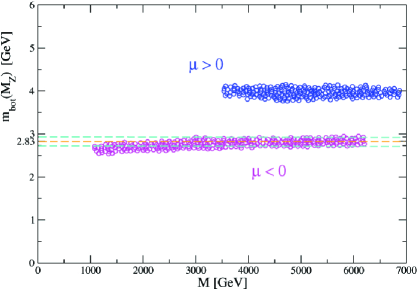
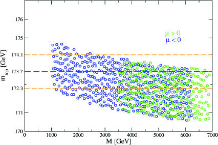
Figure 1: The bottom quark mass at the $Z$ boson scale (left) and top quark pole mass (right) are shown as function of $M$ for both signs of $\mu$.

As was already mentioned, for the lightest Higgs boson mass we used the code FeynHiggs (2.14.0 beta). The prediction for $M_{h}$ of $SU(5)$-FUT with $\mu<0$ is shown in Fig.2, in a range where the unified gaugino mass varies from $0.5~{}{\rm TeV}\lesssim M\lesssim 9~{}{\rm TeV}$. The green points include the $B$-physics constraints. One should keep in mind that these predictions are subject to a theory uncertainty of 3(2) GeV [118]. Older analysis, including in particular less refined evaluations of the light Higgs boson mass, are given in Refs. [46, 124, 125].

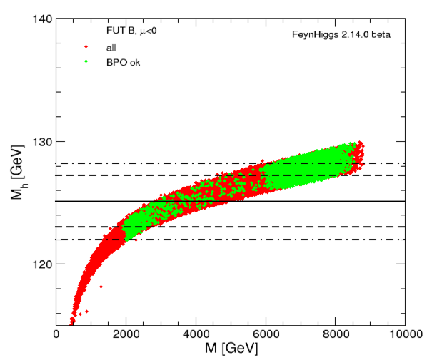
Figure 2: The lightest Higgs mass, $M_{h}$, as a function of $M$ for the FUT model with $\mu<0$. The green points are the ones that satisfy the $B$-physics constraints.

The allowed values of the Higgs mas put a limit on the allowed values of the SUSY masses, as can be seen in Fig.3. In the left (right) plot we impose $M_{h}=125.1\pm 3.1(2.1)~{}{\rm GeV}$ as discussed above. In particular very heavy coloured SUSY particles are favoured (nearly independent of the $M_{h}$ uncertainty), in agreement with the non-observation of those particles at the LHC [126]. Overall, the allowed coloured SUSY masses would remain unobservable at the (HL-)LHC, the ILC or CLIC. However, the coloured spectrum would be accessible at the FCC-hh [127], as could the full heavy Higgs boson spectrum. On the other hand, the lightest observable SUSY particle (LSOP) is the scalar tau. Some parts of the allowed spectrum of the lighter scalar tau or the lighter charginos/neutralinos might be accessible at CLIC with $\sqrt{s}=3~{}{\rm TeV}$.

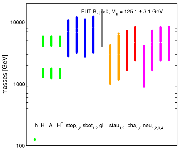
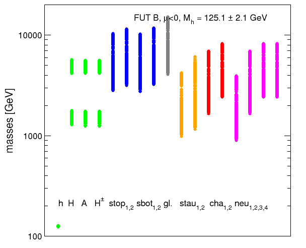
Figure 3: The left (right) plot shows the spectrum of the $SU(5)$-FUT (with $\mu<0$) model after imposing the constraint $M_{h}=125.1\pm 3.1(2.1)~{}{\rm GeV}$. The light (green) points are the various Higgs boson masses, the dark (blue) points following are the two scalar top and bottom masses, the gray ones are the gluino masses, then come the scalar tau masses in orange (light gray), the darker (red) points to the right are the two chargino masses followed by the lighter shaded (pink) points indicating the neutralino masses.

$\delta M_{h}=2.1$	$M_{h}$	$M_{H}$	$M_{A}$	$M_{H^{\pm}}$	$m_{\tilde{t}_{1}}$	$m_{\tilde{t}_{2}}$	$m_{\tilde{b}_{1}}$	$m_{\tilde{b}_{2}}$	$m_{\tilde{g}}$
lightest	123.1	1533	1528	1527	2800	3161	2745	3219	4077
heaviest	127.2	4765	4737	4726	10328	11569	10243	11808	15268
	$m_{\tilde{\tau}_{1}}$	$m_{\tilde{\tau}_{2}}$	$m_{\tilde{\chi}^{\pm}_{1}}$	$m_{\tilde{\chi}^{\pm}_{2}}$	$m_{\tilde{\chi}^{0}_{1}}$	$m_{\tilde{\chi}^{0}_{2}}$	$m_{\tilde{\chi}^{0}_{3}}$	$m_{\tilde{\chi}^{0}_{4}}$	$\tan\beta$
lightest	983	1163	1650	2414	900	1650	2410	2414	45
heaviest	4070	5141	6927	8237	3920	6927	8235	8237	46

$\delta M_{h}=3.1$	$M_{h}$	$M_{H}$	$M_{A}$	$M_{H^{\pm}}$	$m_{\tilde{t}_{1}}$	$m_{\tilde{t}_{2}}$	$m_{\tilde{b}_{1}}$	$m_{\tilde{b}_{2}}$	$m_{\tilde{g}}$
lightest	122.8	1497	1491	1490	2795	3153	2747	3211	4070
heaviest	127.9	4147	4113	4103	10734	12049	11077	12296	16046
	$m_{\tilde{\tau}_{1}}$	$m_{\tilde{\tau}_{2}}$	$m_{\tilde{\chi}^{\pm}_{1}}$	$m_{\tilde{\chi}^{\pm}_{2}}$	$m_{\tilde{\chi}^{0}_{1}}$	$m_{\tilde{\chi}^{0}_{2}}$	$m_{\tilde{\chi}^{0}_{3}}$	$m_{\tilde{\chi}^{0}_{4}}$	$\tan\beta$
lightest	1001	1172	1647	2399	899	647	2395	2399	44
heaviest	4039	6085	7300	8409	4136	7300	8406	8409	45

Table 1: Two example spectra of the $SU(5)$-FUT (with $\mu<0$) . All masses are in GeV and rounded to 1 (0.1) GeV (for the light Higgs mass).

In Table 1 we show two example spectra of the $SU(5)$-FUT (with $\mu<0$)  which span the mass range of the parameter space that is in agreement with the $B$-physics observables and the Higgs-boson mass measurement. We give the lightest and the heaviest spectrum for $\delta M_{h}=2.1$ and $\delta M_{h}=3.1$, respectively. The four Higgs boson masses are denoted as $M_{h}$, $M_{H}$, $M_{A}$ and $M_{H^{\pm}}$. $m_{\tilde{t}_{1,2}}$, $m_{\tilde{t}_{1,2}}$, $m_{\tilde{g}}$, $m_{\tilde{\tau}_{1,2}}$, are the scalar top, scalar bottom, gluino and scalar tau masses, respectively. $m_{\tilde{\chi}^{\pm}_{1,2}}$ and $m_{\tilde{\chi}^{0}_{1,2,3,4}}$ denote the chargino and neutralino masses.

We find that no point of $SU(5)$-FUT (with $\mu<0$) fulfills the strict bound of Eq. (77). (For our evaluation we have used the code MicroMegas [128, 129, 130].) Consequently, on a more general basis a mechanism is needed in our model to reduce the CDM abundance in the early universe. This issue could, for instance, be related to another problem, that of neutrino masses. This type of masses cannot be generated naturally within the class of finite unified theories that we are considering in this paper, although a non-zero value for neutrino masses has clearly been established [103]. However, the class of FUTs discussed here can, in principle, be easily extended by introducing bilinear R-parity violating terms that preserve finiteness and introduce the desired neutrino masses [131, 132, 133]. R-parity violation [134] would have a small impact on the collider phenomenology presented here (apart from the fact that SUSY search strategies could not rely on a ‘missing energy’ signature), but remove the CDM bound of Eq. (77) completely. The details of such a possibility in the present framework attempting to provide the models with realistic neutrino masses will be discussed elsewhere. Other mechanisms, not involving R-parity violation (and keeping the ‘missing energy’ signature), that could be invoked if the amount of CDM appears to be too large, concern the cosmology of the early universe. For instance, “thermal inflation” [135] or “late time entropy injection” [136] could bring the CDM density into agreement with the WMAP measurements. This kind of modifications of the physics scenario neither concerns the theory basis nor the collider phenomenology, but could have a strong impact on the CDM bounds. (Lower values than those permitted by Eq. (77) are naturally allowed if another particle than the lightest neutralino constitutes CDM.)

8 Conclusions

The MSSM is considered a very attractive candidate for describing physics beyond the SM. However, the serious problem of the SM having too many free parameters is further proliferated in the MSSM. Assuming a GUT beyond the scale of gauge coupling unification, based on the idea that a Particle Physics Theory should be more symmetric at higher scales, seems to fit to the MSSM. On the other hand, the unification scenario seems to be unable to further reduce the number of free parameters.

Attempting to reduce the free parameters of a theory, a new approach was proposed in Refs. [18, 19] based on the possible existence of RGI relations among couplings. Although this approach could uncover further symmetries, its application opens new horizons too. At least the Finite Unified Theories seem to be a very promising field for applying the reduction approach. In the FUT case, the discovery of RGI relations among couplings above the unification scale ensures at the same time finiteness to all orders.

The discussion in the previous sections of this paper shows that the predictions of the particular FUT discussed here are impressive. In addition, one could add some comments on a successful FUT from the theoretical side, too. The developments on treating the problem of divergencies include string and non-commutative theories, as well as $N=4$ SUSY theories [137, 138], $N=8$ supergravity [139, 140, 141, 142, 143] and the AdS/CFT correspondence [144]. It is very interesting that the $N=1$ FUT discussed here includes many ideas which survived phenomenological and theoretical tests as well as the ultraviolet divergence problem. It is actually solving that problem in a minimal way.

We concentrated our examination on the predictions of one particular $SU(5)$ Finite Unified Theory, including the restrictions of third generation quark masses and $B$-physics observables. The model, $SU(5)$-FUT (with $\mu<0$), is consistent with all the phenomenological constraints. Compared to our previous analyses [46, 47, 124, 125], the improved evaluation of $M_{h}$ prefers a heavier (Higgs) spectrum and thus in general allows only a very heavy SUSY spectrum. The coloured spectrum could easily escape the (HL-)LHC searches, but can likely be tested at the FCC-hh. The lower part of the electroweak spectrum could be accessible at CLIC.

Acknowledgements

We thank H. Bahl, T. Hahn, W. Hollik, D. Lüst and E. Seiler for helpful discussions. The work of S.H. is supported in part by the MEINCOP Spain under contract FPA2016-78022-P, in part by the Spanish Agencia Estatal de Investigación (AEI) and the EU Fondo Europeo de Desarrollo Regional (FEDER) through the project FPA2016-78645-P, and in part by the AEI through the grant IFT Centro de Excelencia Severo Ochoa SEV-2016-0597. The work of M.M. is partly supported by UNAM PAPIIT through grant IN111518. The work of N.T. and G.Z. are supported by the COST actions CA15108 and CA16201. G.Z. thanks the MPI Munich for hospitality and the A.v.Humboldt Foundation for support.

References

- [1] ATLAS Collaboration, G. Aad et al., Phys.Lett. B716, 1 (2012), arXiv:1207.7214.
- [2] CMS Collaboration, S. Chatrchyan et al., Phys.Lett. B716, 30 (2012), arXiv:1207.7235.
- [3] ATLAS Collaboration, (2013), ATLAS-CONF-2013-014, ATLAS-COM-CONF-2013-025.
- [4] CMS Collaboration, S. Chatrchyan et al., (2013), arXiv:1303.4571.
- [5] J. C. Pati and A. Salam, Phys. Rev. Lett. 31, 661 (1973).
- [6] H. Georgi and S. L. Glashow, Phys. Rev. Lett. 32, 438 (1974).
- [7] H. Georgi, H. R. Quinn, and S. Weinberg, Phys. Rev. Lett. 33, 451 (1974).
- [8] H. Georgi, Particles and Fields: Williamsburg 1974. AIP Conference Proceedings No. 23, American Institute of Physics, New York, 1974, ed. Carlson, C. E.
- [9] H. Fritzsch and P. Minkowski, Ann. Phys. 93, 193 (1975).
- [10] S. Dimopoulos and H. Georgi, Nucl. Phys. B193, 150 (1981).
- [11] N. Sakai, Zeit. Phys. C11, 153 (1981).
- [12] U. Amaldi, W. de Boer, and H. Furstenau, Phys. Lett. B260, 447 (1991).
- [13] A. J. Buras, J. R. Ellis, M. K. Gaillard, and D. V. Nanopoulos, Nucl. Phys. B135, 66 (1978).
- [14] J. Kubo, M. Mondragon, M. Olechowski, and G. Zoupanos, Nucl. Phys. B479, 25 (1996), arXiv:hep-ph/9512435.
- [15] J. Kubo, M. Mondragon, and G. Zoupanos, Acta Phys. Polon. B27, 3911 (1997), arXiv:hep-ph/9703289.
- [16] T. Kobayashi, J. Kubo, M. Mondragon, and G. Zoupanos, Acta Phys. Polon. B30, 2013 (1999).
- [17] P. Fayet, Nucl. Phys. B149, 137 (1979).
- [18] W. Zimmermann, Commun. Math. Phys. 97, 211 (1985).
- [19] R. Oehme and W. Zimmermann, Commun. Math. Phys. 97, 569 (1985).
- [20] D. Kapetanakis, M. Mondragon, and G. Zoupanos, Z. Phys. C60, 181 (1993), arXiv:hep-ph/9210218.
- [21] J. Kubo, M. Mondragon, and G. Zoupanos, Nucl. Phys. B424, 291 (1994).
- [22] J. Kubo, M. Mondragon, N. D. Tracas, and G. Zoupanos, Phys. Lett. B342, 155 (1995), arXiv:hep-th/9409003.
- [23] J. Kubo, M. Mondragon, M. Olechowski, and G. Zoupanos, (1995), arXiv:hep-ph/9510279.
- [24] M. Mondragon and G. Zoupanos, Nucl. Phys. Proc. Suppl. 37C, 98 (1995).
- [25] J. Kubo, M. Mondragon, and G. Zoupanos, Phys. Lett. B389, 523 (1996), arXiv:hep-ph/9609218.
- [26] J. Kubo, M. Mondragon, S. Shoda, and G. Zoupanos, Nucl. Phys. B469, 3 (1996), arXiv:hep-ph/9512258.
- [27] O. Piguet and K. Sibold, Int. J. Mod. Phys. A1, 913 (1986).
- [28] C. Lucchesi, O. Piguet, and K. Sibold, Helv. Phys. Acta 61, 321 (1988).
- [29] C. Lucchesi and G. Zoupanos, Fortschr. Phys. 45, 129 (1997), arXiv:hep-ph/9604216.
- [30] I. Jack and D. R. T. Jones, Phys. Lett. B349, 294 (1995), arXiv:hep-ph/9501395.
- [31] W. Zimmermann, Commun.Math.Phys. 219, 221 (2001).
- [32] M. Mondragón, N. Tracas, and G. Zoupanos, Phys.Lett. B728, 51 (2014), arXiv:1309.0996.
- [33] S. Heinemeyer, M. Mondragon and G. Zoupanos, JHEP 0807 (2008) 135 doi:10.1088/1126-6708/2008/07/135 [arXiv:0712.3630 [hep-ph]].
- [34] D. R. T. Jones, L. Mezincescu and Y. P. Yao, Phys. Lett. B148, 317 (1984).
- [35] I. Jack and D. R. T. Jones, Phys. Lett. B333, 372 (1994), [hep-ph/9405233].
- [36] L. E. Ibanez and D. Lust, Nucl. Phys. B 382 (1992) 305 doi:10.1016/0550-3213(92)90189-I [hep-th/9202046].
- [37] V. S. Kaplunovsky and J. Louis, Phys. Lett. B 306 (1993) 269 doi:10.1016/0370-2693(93)90078-V [hep-th/9303040].
- [38] A. Brignole, L. E. Ibanez and C. Munoz, Nucl. Phys. B 422 (1994) 125 Erratum: [Nucl. Phys. B 436 (1995) 747] doi:10.1016/0550-3213(94)00600-J, 10.1016/0550-3213(94)00068-9 [hep-ph/9308271].
- [39] J. A. Casas, A. Lleyda and C. Munoz, Phys. Lett. B 380 (1996) 59 doi:10.1016/0370-2693(96)00489-3 [hep-ph/9601357].
- [40] Y. Kawamura, T. Kobayashi and J. Kubo, Phys. Lett. B 405, 64 (1997) [arXiv:hep-ph/9703320].
- [41] T. Kobayashi, J. Kubo and G. Zoupanos, Phys. Lett. B 427 (1998) 291 doi:10.1016/S0370-2693(98)00343-8 [hep-ph/9802267].
- [42] T. Kobayashi, J. Kubo, M. Mondragon and G. Zoupanos, Nucl. Phys. B 511, 45 (1998) [arXiv:hep-ph/9707425].
- [43] V. A. Novikov, M. A. Shifman, A. I. Vainshtein and V. I. Zakharov, Nucl. Phys. B229, 407 (1983).
- [44] V. A. Novikov, M. A. Shifman, A. I. Vainshtein and V. I. Zakharov, Phys. Lett. B166, 329 (1986).
- [45] M. A. Shifman, Int. J. Mod. Phys. A11, 5761 (1996), [hep-ph/9606281].
- [46] S. Heinemeyer, M. Mondragon and G. Zoupanos, Phys. Lett. B 718 (2013) 1430 doi:10.1016/j.physletb.2012.12.042 [arXiv:1211.3765 [hep-ph]].
- [47] S. Heinemeyer, M. Mondragon and G. Zoupanos, Fortsch. Phys. 61 (2013) no.11, 969 doi:10.1002/prop.201300017 [arXiv:1305.5073 [hep-ph]].
- [48] S. Heinemeyer, M. Mondragon and G. Zoupanos, Int. J. Mod. Phys. A 29 (2014) 1430032 doi:10.1142/S0217751X14300324 [arXiv:1412.5766 [hep-ph]].
- [49] R. Oehme, Prog. Theor. Phys. Suppl. 86, 215 (1986).
- [50] J. Kubo, K. Sibold and W. Zimmermann, Nucl. Phys. B259, 331 (1985).
- [51] J. Kubo, K. Sibold and W. Zimmermann, Phys. Lett. B220, 185 (1989).
- [52] O. Piguet and K. Sibold, Phys. Lett. 229B, 83 (1989).
- [53] P. Breitenlohner and D. Maison, Commun. Math. Phys. 219, 179 (2001).
- [54] J. Wess and B. Zumino, Phys. Lett. B49, 52 (1974).
- [55] J. Iliopoulos and B. Zumino, Nucl. Phys. B76, 310 (1974).
- [56] K. Fujikawa and W. Lang, Nucl. Phys. B88, 61 (1975).
- [57] A. Parkes and P. C. West, Phys. Lett. B138, 99 (1984).
- [58] S. Rajpoot and J. G. Taylor, Phys. Lett. B147, 91 (1984).
- [59] S. Rajpoot and J. G. Taylor, Int. J. Theor. Phys. 25, 117 (1986).
- [60] P. C. West, Phys. Lett. B137, 371 (1984).
- [61] D. R. T. Jones and L. Mezincescu, Phys. Lett. B138, 293 (1984).
- [62] D. R. T. Jones and A. J. Parkes, Phys. Lett. B160, 267 (1985).
- [63] A. J. Parkes, Phys. Lett. B156, 73 (1985).
- [64] L. O’Raifeartaigh, Nucl. Phys. B96, 331 (1975).
- [65] P. Fayet and J. Iliopoulos, Phys. Lett. B51, 461 (1974).
- [66] C. Lucchesi, O. Piguet and K. Sibold, Phys. Lett. B201, 241 (1988).
- [67] S. Ferrara and B. Zumino, Nucl. Phys. B87, 207 (1975).
- [68] O. Piguet and K. Sibold, Nucl. Phys. B196, 428 (1982).
- [69] O. Piguet and K. Sibold, Nucl. Phys. B196, 447 (1982).
- [70] O. Piguet and K. Sibold, Phys. Lett. B177, 373 (1986).
- [71] P. Ensign and K. T. Mahanthappa, Phys. Rev. D36, 3148 (1987).
- [72] O. Piguet, hep-th/9606045, talk given at “10th International Conference on Problems of Quantum Field Theory”.
- [73] L. Alvarez-Gaume and P. H. Ginsparg, Nucl. Phys. B243, 449 (1984).
- [74] W. A. Bardeen and B. Zumino, Nucl. Phys. B244, 421 (1984).
- [75] B. Zumino, Y.-S. Wu and A. Zee, Nucl. Phys. B239, 477 (1984).
- [76] R. G. Leigh and M. J. Strassler, Nucl. Phys. B447, 95 (1995), [hep-th/9503121].
- [77] M. Mondragon and G. Zoupanos, Acta Phys. Polon. B34, 5459 (2003).
- [78] R. Delbourgo, Nuovo Cim. A 25, 646 (1975).
- [79] A. Salam and J. A. Strathdee, Nucl. Phys. B 86, 142 (1975).
- [80] M. T. Grisaru, W. Siegel and M. Rocek, Nucl. Phys. B 159, 429 (1979).
- [81] L. Girardello and M. T. Grisaru, Nucl. Phys. B 194, 65 (1982).
- [82] J. Hisano and M. A. Shifman, Phys. Rev. D56, 5475 (1997), [hep-ph/9705417].
- [83] I. Jack and D. R. T. Jones, Phys. Lett. B415, 383 (1997), [hep-ph/9709364].
- [84] L. V. Avdeev, D. I. Kazakov and I. N. Kondrashuk, Nucl. Phys. B510, 289 (1998), [hep-ph/9709397].
- [85] D. I. Kazakov, Phys. Lett. B449, 201 (1999), [hep-ph/9812513].
- [86] D. I. Kazakov, Phys. Lett. B421, 211 (1998), [hep-ph/9709465].
- [87] I. Jack, D. R. T. Jones and A. Pickering, Phys. Lett. B426, 73 (1998), [hep-ph/9712542].
- [88] I. Jack and D. R. T. Jones, Phys. Lett. B 465 (1999) 148 doi:10.1016/S0370-2693(99)01064-3 [hep-ph/9907255].
- [89] T. Kobayashi, J. Kubo, M. Mondragon and G. Zoupanos, AIP Conf. Proc. 490 (1999) no.1, 279. doi:10.1063/1.1301389
- [90] A. Karch, T. Kobayashi, J. Kubo and G. Zoupanos, Phys. Lett. B 441 (1998) 235 doi:10.1016/S0370-2693(98)01182-4 [hep-th/9808178].
- [91] M. Mondragon and G. Zoupanos, J. Phys. Conf. Ser. 171 (2009) 012095. doi:10.1088/1742-6596/171/1/012095
- [92] S. Hamidi and J. H. Schwarz, Phys. Lett. 147B (1984) 301. doi:10.1016/0370-2693(84)90121-7
- [93] D. R. T. Jones and S. Raby, Phys. Lett. 143B (1984) 137. doi:10.1016/0370-2693(84)90820-7
- [94] J. Leon, J. Perez-Mercader, M. Quiros and J. Ramirez-Mittelbrunn, Phys. Lett. 156B (1985) 66. doi:10.1016/0370-2693(85)91356-5
- [95] M. Misiak et al., Phys. Rev. Lett. 98, 022002 (2007) [arXiv:hep-ph/0609232]; M. Ciuchini, G. Degrassi, P. Gambino and G. F. Giudice, Nucl. Phys. B 534, 3 (1998) [arXiv:hep-ph/9806308]; G. Degrassi, P. Gambino and G. F. Giudice, JHEP 0012, 009 (2000) [arXiv:hep-ph/0009337]; M. S. Carena, D. Garcia, U. Nierste and C. E. M. Wagner, Phys. Lett. B 499, 141 (2001) [arXiv:hep-ph/0010003]; G. D’Ambrosio, G. F. Giudice, G. Isidori and A. Strumia, Nucl. Phys. B 645, 155 (2002) [arXiv:hep-ph/0207036].
- [96] The Heavy Flavor Averaging Group, D. Asner et al., arXiv:1010.1589 [hep-ex], with updates available at http://www.slac.stanford.edu/xorg/hfag/osc .
- [97] A. J. Buras, Phys. Lett. B 566, 115 (2003) [arXiv:hep-ph/0303060]; G. Isidori and D. M. Straub, Eur. Phys. J. C 72, 2103 (2012) [arXiv:1202.0464 [hep-ph]].
- [98] C. Bobeth, M. Gorbahn, T. Hermann, M. Misiak, E. Stamou and M. Steinhauser, arXiv:1311.0903 [hep-ph]; T. Hermann, M. Misiak and M. Steinhauser, arXiv:1311.1347 [hep-ph]; C. Bobeth, M. Gorbahn and E. Stamou, arXiv:1311.1348 [hep-ph].
- [99] R.Aaij et al. [LHCb Collaboration], Phys. Rev. Lett. 111, 101805 (2013) [arXiv:1307.5024 [hep-ex]].
- [100] S. Chatrchyan et al. [CMS Collaboration], Phys. Rev. Lett. 111, 101804 (2013) [arXiv:1307.5025 [hep-ex]].
- [101] R.Aaij et al. [LHCb and CMS Collaborations], LHCb-CONF-2013-012, CMS PAS BPH-13-007.
- [102] G. Isidori and P. Paradisi, Phys. Lett. B 639, 499 (2006) [arXiv:hep-ph/0605012]; G. Isidori, F. Mescia, P. Paradisi and D. Temes, Phys. Rev. D 75, 115019 (2007) [arXiv:hep-ph/0703035], and references therein.
- [103] K. A. Olive et al. [Particle Data Group Collaboration], Chin. Phys. C 38, 090001 (2014).
- [104] A. J. Buras, P. Gambino, M. Gorbahn, S. Jager and L. Silvestrini, Nucl. Phys. B 592, 55 (2001) [arXiv:hep-ph/0007313].
- [105] R. Aaij et al. [LHCb Collaboration], New J. Phys. 15, 053021 (2013) [arXiv:1304.4741 [hep-ex]].
- [106] H. Goldberg, Phys. Rev. Lett. 50, 1419 (1983); J. Ellis, J. Hagelin, D. Nanopoulos, K. Olive and M. Srednicki, Nucl. Phys. B 238, 453 (1984).
- [107] E. Komatsu et al. [WMAP Collaboration], Astrophys. J. Suppl. 192 (2011) 18 doi:10.1088/0067-0049/192/2/18 [arXiv:1001.4538 [astro-ph.CO]].
- [108] E. Komatsu et al. [WMAP Science Team], PTEP 2014 (2014) 06B102 doi:10.1093/ptep/ptu083 [arXiv:1404.5415 [astro-ph.CO]].
- [109] S. Heinemeyer, Int. J. Mod. Phys. A 21, 2659 (2006) [arXiv:hep-ph/0407244].
- [110] S. Heinemeyer, W. Hollik and G. Weiglein, Phys. Rept. 425, 265 (2006) [arXiv:hep-ph/0412214].
- [111] A. Djouadi, Phys. Rept. 459, 1 (2008) [arXiv:hep-ph/0503173].
- [112] ATLAS Collaboration, G. Aad et al., Phys. Lett. B 716, 1 (2012) [arXiv:1207.7214 [hep-ex]].
- [113] CMS Collaboration, S. Chatrchyan et al., Phys. Lett. B 716, 30 (2012) [arXiv:1207.7235 [hep-ex]].
- [114] S. Heinemeyer, O. Stål and G. Weiglein, Phys. Lett. B 710, 201 (2012) [arXiv:1112.3026 [hep-ph]].
- [115] P. Bechtle, S. Heinemeyer, O. Stål, T. Stefaniak, G. Weiglein and L. Zeune, Eur. Phys. J. C 73, 2354 (2013) [arXiv:1211.1955 [hep-ph]].
- [116] P. Bechtle et al., Eur. Phys. J. C 77, no.2, 67 (2017) [arXiv:1608.00638 [hep-ph]].
- [117] G. Aad et al. [ATLAS and CMS Collaborations], Phys. Rev. Lett. 114, 191803 (2015) [arXiv:1503.07589 [hep-ex]].
- [118] G. Degrassi, S. Heinemeyer, W. Hollik, P. Slavich and G. Weiglein, Eur. Phys. J. C28, 133 (2003) [arXiv:hep-ph/0212020].
- [119] O. Buchmueller et al., Eur. Phys. J. C 74, no.3, 2809 (2014) [arXiv:1312.5233 [hep-ph]].
- [120] H. Bahl, S. Heinemeyer, W. Hollik and G. Weiglein, arXiv:1706.00346 [hep-ph].
- [121] S. Heinemeyer, W. Hollik and G. Weiglein, Comput. Phys. Commun. 124, 76 (2000) [arXiv:hep-ph/9812320]; S. Heinemeyer, W. Hollik and G. Weiglein, Eur. Phys. J. C 9, 343 (1999) [arXiv:hep-ph/9812472]; M. Frank et al., JHEP 0702, 047 (2007) [arXiv:hep-ph/0611326]; T. Hahn, S. Heinemeyer, W. Hollik, H. Rzehak and G. Weiglein, Comput. Phys. Commun. 180, 1426 (2009); T. Hahn, S. Heinemeyer, W. Hollik, H. Rzehak and G. Weiglein, Phys. Rev. Lett. 112, 14, 141801 (2014) [arXiv:1312.4937 [hep-ph]]; H. Bahl and W. Hollik, Eur. Phys. J. C 76, 499 (2016) [arXiv:1608.01880 [hep-ph]]. See http://www.feynhiggs.de .
- [122] [ATLAS and CDF and CMS and D0 Collaborations], arXiv:1403.4427 [hep-ex].
- [123] M. Carena, D. Garcia, U. Nierste and C. E. M. Wagner, Nucl. Phys. B 577 (2000) 88 doi:10.1016/S0550-3213(00)00146-2 [hep-ph/9912516].
- [124] S. Heinemeyer, M. Mondragon and G. Zoupanos, Int. J. Mod. Phys. Conf. Ser. 13 (2012) 118. doi:10.1142/S2010194512006782
- [125] S. Heinemeyer, M. Mondragon and G. Zoupanos, Phys. Part. Nucl. 44 (2013) 299. doi:10.1134/S1063779613020159
- [126] https://twiki.cern.ch/twiki/bin/view/AtlasPublic/SupersymmetryPublicResults, https://twiki.cern.ch/twiki/bin/view/CMSPublic/PhysicsResultsSUS
- [127] M. Mangano, CERN Yellow Report CERN 2017-003-M [arXiv:1710.06353 [hep-ph]].
- [128] G. Belanger, F. Boudjema, A. Pukhov and A. Semenov, Comput. Phys. Commun. 149 (2002) 103 doi:10.1016/S0010-4655(02)00596-9 [hep-ph/0112278].
- [129] G. Belanger, F. Boudjema, A. Pukhov and A. Semenov, Comput. Phys. Commun. 174 (2006) 577 doi:10.1016/j.cpc.2005.12.005 [hep-ph/0405253].
- [130] D. Barducci, G. Belanger, J. Bernon, F. Boudjema, J. Da Silva, S. Kraml, U. Laa and A. Pukhov, Comput. Phys. Commun. 222 (2018) 327 doi:10.1016/j.cpc.2017.08.028 [arXiv:1606.03834 [hep-ph]].
- [131] J. W. F. Valle, PoS corfu 98 (1998) 010 [hep-ph/9907222].
- [132] J. Valle, arXiv:hep-ph/9907222 and references therein.
- [133] M. Diaz, M. Hirsch, W. Porod, J. Romao and J. Valle, Phys. Rev. D68 (2003) 013009 [Erratum-ibid. D71 (2005) 059904] [arXiv:hep-ph/0302021].
-
[134]
H. Dreiner,
arXiv:hep-ph/9707435;
G. Bhattacharyya, arXiv:hep-ph/9709395;
B. Allanach, A. Dedes and H. Dreiner, Phys. Rev. D 60 (1999) 075014 [arXiv:hep-ph/9906209];
J. Romao and J. Valle, Nucl. Phys. B 381 (1992) 87; - [135] D. Lyth and E. Stewart, Phys. Rev. D 53 (1996) 1784 [arXiv:hep-ph/9510204].
- [136] G. Gelmini and P. Gondolo, Phys. Rev. D74 (2006) 023510 [arXiv:hep-ph/0602230].
- [137] S. Mandelstam, Nucl. Phys. B 213 (1983) 149. doi:10.1016/0550-3213(83)90179-7
- [138] L. Brink, O. Lindgren and B. E. W. Nilsson, Phys. Lett. 123B (1983) 323. doi:10.1016/0370-2693(83)91210-8
- [139] Z. Bern, J. J. Carrasco, L. J. Dixon, H. Johansson and R. Roiban, Phys. Rev. Lett. 103 (2009) 081301 doi:10.1103/PhysRevLett.103.081301 [arXiv:0905.2326 [hep-th]].
- [140] R. Kallosh, JHEP 0909 (2009) 116 doi:10.1088/1126-6708/2009/09/116 [arXiv:0906.3495 [hep-th]].
- [141] Z. Bern, J. J. Carrasco, L. J. Dixon, H. Johansson, D. A. Kosower and R. Roiban, Phys. Rev. Lett. 98 (2007) 161303 doi:10.1103/PhysRevLett.98.161303 [hep-th/0702112].
- [142] Z. Bern, L. J. Dixon and R. Roiban, Phys. Lett. B 644 (2007) 265 doi:10.1016/j.physletb.2006.11.030 [hep-th/0611086].
- [143] M. B. Green, J. G. Russo and P. Vanhove, Phys. Rev. Lett. 98 (2007) 131602 doi:10.1103/PhysRevLett.98.131602 [hep-th/0611273].
- [144] J. M. Maldacena, Int. J. Theor. Phys. 38 (1999) 1113 [Adv. Theor. Math. Phys. 2 (1998) 231] doi:10.1023/A:1026654312961, 10.4310/ATMP.1998.v2.n2.a1 [hep-th/9711200].