Hypersingular nonlinear boundary-value problems
with a small parameter^∗∗∗

Abstract

For the first time, some hypersingular nonlinear boundary-value problems with a small parameter $\varepsilon$ at the highest derivative are described. These problems essentially (qualitatively and quantitatively) differ from the usual linear and quasilinear singularly perturbed boundary-value problems and have the following unusual properties:

(i) in hypersingular boundary-value problems, super thin boundary layers arise, and the derivative at the boundary layer can have very large values of the order of $e^{1/\varepsilon}$ and more (in standard problems with boundary layers, the derivative at the boundary has the order of $\varepsilon^{-1}$ or less);

(ii) in hypersingular boundary-value problems, the position of the boundary layer is determined by the values of the unknown function at the boundaries (in standard problems with boundary layers, the position of the boundary layer is determined by coefficients of the given equation, and the values of the unknown function at the boundaries do not play a role here);

(iii) hypersingular boundary-value problems do not admit a direct application of the method of matched asymptotic expansions (without a preliminary nonlinear point transformation of the equation under consideration).

Examples of hypersingular nonlinear boundary-value problems with ODEs and PDEs are given and their exact solutions are obtained. It is important to note that the exact solutions presented in this paper can be used to compare the effectiveness of various methods of numerical integration of singularly perturbed problems with boundary layers, and also to develop new numerical and approximate analytical methods.

1 Introduction

Singularly perturbed boundary-value problems with a small parameter at the highest derivative are often encountered in hydro- and aerodynamics, theory of mass and heat transfer, theory of elasticity, nonlinear mechanics and other applications. An important qualitative feature of singular boundary-value problems is that for the zero value of a small parameter the order of the differential equation under consideration decreases and some parts of the boundary conditions cannot be satisfied. Various problems and solution methods for ODEs and PDEs with a small parameter at the highest derivative are described, for example, in [1, 2, 3, 4, 5, 6, 7, 8, 9, 10, 11, 12, 13].

For singularly perturbed quasilinear boundary-value problems of the form

$$\varepsilon y^{\prime\prime}_{xx}+py^{\prime}_{x}+q(x,y)=0\quad\ (0<x<1);\quad\ y(0)=\alpha,\quad\ y(1)=\beta$$ (1)

with a small parameter $\varepsilon$, the position of the boundary layer is determined by the sign of the coefficient $p$. For $p>0$, the boundary layer is formed at the left boundary near the point $x=0$, for $p<0$, at the right boundary near the point $x=1$. An analogous situation holds for more complex singularly perturbed quasilinear boundary-value problems of the form (1) with $p=p(x)$.

We note that for $p>0$ and $\varepsilon\to 0$ the derivative of the solution of the problem (1) takes large values proportional to $\varepsilon^{-1}$ on the left boundary.

In this article we will consider hypersingular boundary-value problems with a small parameter, the solutions of which qualitatively and quantitatively differ from the solutions of the problems (1).

2 Hypersingular boundary-value problems for ordinary differential
equations with a small parameter

2.1 Example of hypersingular boundary-value problem. Exact solution,
qualitative features

Problem 1. Consider the nonlinear boundary-value problem

$$\varepsilon y^{\prime\prime}_{xx}+p(y^{\prime}_{x})^{2}+qy^{\prime}_{x}=0;$$ (2)

$$y(0)=\alpha,\quad\ y(1)=\beta.$$ (3)

In what follows, we assume that $p>0$, $q>0$ and $\varepsilon>0$ is a small parameter.

Equation (2) admits an exact linearization by means of the transformation $y=(\varepsilon/p)\ln u$ (see also Section 2.2). Its general solution is determined by the formula

$$y=\frac{\mskip 1.0mu\varepsilon\mskip 1.0mu}{\mskip 1.0mup\mskip 1.0mu}\ln(C_{1}+C_{2}e^{-qx/\varepsilon}),$$ (4)

where $C_{1}$ and $C_{2}$ are arbitrary constants.

The exact solution of the boundary-value problem (2)–(3) has the form

$$y=\frac{\mskip 1.0mu\varepsilon\mskip 1.0mu}{\mskip 1.0mup\mskip 1.0mu}\ln\biggl{[}\frac{\mskip 1.0mu(e^{\alpha p/\varepsilon}-e^{\beta p/\varepsilon})e^{-qx/\varepsilon}+e^{\beta p/\varepsilon}-e^{(\alpha p-q)/\varepsilon}\mskip 1.0mu}{\mskip 1.0mu1-e^{-q/\varepsilon}\mskip 1.0mu}\biggr{]}.$$ (5)

Let us find the derivatives on the left and right boundaries:

$$y^{\prime}_{x}|_{x=0}=\frac{\mskip 1.0muq\mskip 1.0mu}{\mskip 1.0mup\mskip 1.0mu}\frac{\mskip 1.0mue^{(\beta-\alpha)p/\varepsilon}-1\mskip 1.0mu}{\mskip 1.0mu1-e^{-q/\varepsilon}\mskip 1.0mu},\quad\ y^{\prime}_{x}|_{x=1}=\frac{\mskip 1.0muq\mskip 1.0mu}{\mskip 1.0mup\mskip 1.0mu}\frac{\mskip 1.0mu1-e^{(\alpha-\beta)p/\varepsilon}\mskip 1.0mu}{\mskip 1.0mue^{q/\varepsilon}-1\mskip 1.0mu}.$$ (6)

The analysis shows that, depending on the values of the parameters $\alpha$ and $\beta$ (as $\varepsilon\to 0$), the following three qualitatively different situations are possible:

(i) $$\ \beta>\alpha\qquad\qquad\ \ \ \,\,(\text{there is a boundary layer on the left, near $x{=}0$});$$

(ii) $$\ \beta<\alpha-(q/p)\quad\ \ \,(\text{there is a boundary layer on the right, near $x{=}1$});$$ (7)

(iii) $$\ \alpha{-}(q/p)\leq\beta\leq\alpha\ (\text{there is no boundary layer}).$$

On the line $\beta=\alpha$, the problem (2)–(3) has the trivial solution $y=\alpha$, and on the line $\beta=\alpha-(q/p)$ it has the linear solution $y=\alpha-(q/p)x$ (both these solutions are degenerate and do not depend on $\varepsilon$). It is seen from (7) that the position of the boundary layer (or its absence) in the problem under consideration is determined by the boundary values $\alpha$ and $\beta$, which is qualitatively different from the situation typical for standard problems with a boundary layer (see Section 1), where the boundary conditions do not affect the position of the boundary layer.

Fig. 1a represents the curves describing the exact solutions of the problem (2)–(3) and corresponding to the three different cases in (7); they are constructed according to the formula (5) for $p=q=1$ and $\varepsilon=0.1$ and are depicted by the solid line for $\alpha=1$, $\beta=1/2$; by the dashed line for $\alpha=2$, $\beta=0$; by the dash-dotted line for $\alpha=1$, $\beta=1/2$. Fig. 1b represents the plane of the parameters $\alpha$, $\beta$, in which the parts of the plane defining three qualitatively different types of the solutions of the problem (2)–(3) and satisfying the inequalities (i), (ii), (iii) in (7) for $p=q=1$ are shaded in different ways; these parts of the plane are delimited by the straight lines $\beta=\alpha$ and $\beta=\alpha-1$, which correspond to the degenerate solutions.

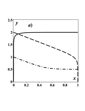
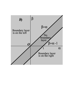
Figure 1: a) Curves constructed using formula (5) for $p=q=1$ and $\varepsilon=0.1$ for $\alpha=0$, $\beta=2$ (solid line); $\alpha=2$, $\beta=0$ (dashed line); $\alpha=1$, $\beta=1/2$ (dash-dotted line); b) regions in the plane of the parameters $\alpha$, $\beta$ with qualitatively different types of solutions of the problem (2)–(3).

We set $p=q=1$, $\alpha=0$, $\beta=1$ in (2)–(3). It follows from the first relation (6) that even for moderately small $\varepsilon=\frac{\mskip 1.0mu1\mskip 1.0mu}{\mskip 1.0mu10\mskip 1.0mu}$ the derivative reaches extremely large values $y^{\prime}_{x}|_{x=0}\simeq e^{1/\varepsilon}\approx 22026.442$ on the left boundary, which corresponds to the hyperfine (hypersingular) boundary layer. For comparison, we note that in the problem (2)–(3) for $p=q=1$, $\alpha=0$, $\beta=1$, $\varepsilon=\frac{\mskip 1.0mu1\mskip 1.0mu}{\mskip 1.0mu20\mskip 1.0mu}$ the derivative on the left boundary will be larger than the derivative on the left boundary in the problem (1) for $p=1$, $q(x,y)=y$, $\alpha=0$, $\beta=1$, $\varepsilon=10^{-8}$.

Similar problems differ fundamentally from the classical problems with a boundary layer (in which the derivative at the boundary is of the order of $\varepsilon^{-1}$ or less) and no such problems have been encountered in the literature (see, for example, [1, 2, 3, 4, 5, 6, 7, 8, 9, 10, 11]). At the present time, there are no effective numerical methods that allow directly (without a preliminary nonlinear point transformation of the given equation) to consider such hypersingular problems even for moderately small $\varepsilon\simeq\frac{\mskip 1.0mu1\mskip 1.0mu}{\mskip 1.0mu50\mskip 1.0mu}$ and, especially, for smaller values of $\varepsilon$.

Remark 1.

A qualitatively similar situation occurs for a hypersingular boundary-value problem described by the equation $\varepsilon y^{\prime\prime}_{xx}+(y^{\prime}_{x})^{2}-1=0$ with the boundary conditions (3).

Remark 2.

Equation (2) describes a family of the traveling wave exact solutions of the potential Burgers equation $u_{t}+u_{z}^{2}=\varepsilon u_{zz}$ [14], in which we have to set $u=-py(x)$, where $x=z-qt$.

Remark 3.

Differential equation (2) do not satisfy the Painlevé test [15, 16].

2.2 Two classes of hypersingular problems admitting linearization

Problem 2. We consider the nonlinear boundary-value problem with a small parameter

$$\varepsilon y^{\prime\prime}_{xx}+p(y^{\prime}_{x})^{2}+q(x)y^{\prime}_{x}+r(x)=0;\quad\ y(0)=\alpha,\quad\ y(1)=\beta,$$ (8)

which generalizes the problem (2)–(3) and contains two arbitrary functions $q(x)$, $r(x)$ and the constant $p$.

The substitution $y=(\varepsilon/p)\ln u$ reduces the problem (8) to the linear problem:

$$\varepsilon^{2}u^{\prime\prime}_{xx}+\varepsilon q(x)u^{\prime}_{x}+pr(x)u=0;\quad\ u(0)=A,\quad\ u(1)=B,$$ (9)

where $A=e^{\alpha p/\varepsilon}$ and $B=e^{\beta p/\varepsilon}$.

If $q(x)=\text{const}$ and $r(x)=\text{const}$, then we can obtain the exact solution of the problem (9). If $q$ and/or $r$ are not constants, then to obtain an approximate solution as $\varepsilon\to 0$ we can use the method of matched asymptotic expansions [1, 2, 3, 4, 5, 7].

Remark 4.

The problem (8), as well as the problem (2)–(3), does not allow a direct application of the method of matched asymptotic expansions (without a preliminary nonlinear point transformation of the equation under consideration), since the second term of this equation remains dominant over the first term with any change in the scale of the independent variable by means of the substitution $x=k\bar{x}$, where $k=k(\varepsilon)$.

Problem 3. The nonlinear boundary-value problem with a small parameter

$$\varepsilon y^{\prime\prime}_{xx}+p(y)(y^{\prime}_{x})^{2}+q(x)y^{\prime}_{x}=0;\quad\ y(0)=\alpha,\quad\ y(1)=\beta,$$ (10)

containing two arbitrary functions $p(y)$ and $q(x)$, with the substitution

$$u=P(y),\quad\ P(y)=\int^{y}_{0}\exp\biggl{[}\frac{\mskip 1.0mu1\mskip 1.0mu}{\mskip 1.0mu\varepsilon\mskip 1.0mu}\int^{z}_{0}p(\xi)\,d\xi\biggr{]}dz,$$ (11)

reduces to the linear problem

$$\varepsilon u^{\prime\prime}_{xx}+q(x)u^{\prime}_{x}=0;\quad\ u(0)=P(\alpha),\quad u(1)=P(\beta),$$ (12)

that is easily integrable.

In particular, for $q=\text{const}$, by using the transformation (11) and equation (12), we obtain the solution of the problem (10) in an implicit form

$$P(y)=\frac{\mskip 1.0muP(\beta)-P(\alpha)e^{-q/\varepsilon}\mskip 1.0mu}{\mskip 1.0mu1-e^{-q/\varepsilon}\mskip 1.0mu}+\frac{\mskip 1.0muP(\alpha)-P(\beta)\mskip 1.0mu}{\mskip 1.0mu1-e^{-q/\varepsilon}\mskip 1.0mu}e^{-qx/\varepsilon}.$$ (13)

Differentiating (13), we find the derivative on the left boundary:

$$y^{\prime}_{x}\bigr{|}_{x=0}=\frac{\mskip 1.0muq\mskip 1.0mu}{\mskip 1.0mu\varepsilon\mskip 1.0mu}\frac{\mskip 1.0muP(\beta)-P(\alpha)\mskip 1.0mu}{\mskip 1.0muP^{\prime}_{y}(\alpha)(1-e^{-q/\varepsilon})\mskip 1.0mu}=\frac{\mskip 1.0muq\mskip 1.0mu}{\mskip 1.0mu\varepsilon\mskip 1.0mu}\frac{\mskip 1.0muP(\beta)-P(\alpha)\mskip 1.0mu}{\mskip 1.0mu(1-e^{-q/\varepsilon})\mskip 1.0mu}\exp\biggl{[}-\frac{\mskip 1.0mu1\mskip 1.0mu}{\mskip 1.0mu\varepsilon\mskip 1.0mu}\int^{\alpha}_{0}p(\xi)\,d\xi\biggr{]}.$$ (14)

Remark 5.

In the problem (10) and the formulas (11), (13)–(14), the functions $p(y)$ and $q(x)$ may also depend on the small parameter $\varepsilon$.

Example. We consider the problem (10) for $p(y)=e^{y}+\varepsilon$, $q(x)=1$, $\beta>0$, $\alpha=0$ ($\varepsilon\to 0$). Substituting these functions and constants in (14), we obtain a very large derivative on the boundary

$$y^{\prime}_{x}\bigr{|}_{x=0}=\frac{\mskip 1.0mu1\mskip 1.0mu}{\mskip 1.0mu1-e^{-1/\varepsilon}\mskip 1.0mu}\biggl{[}\exp\biggl{(}\frac{\mskip 1.0mue^{\beta}-1\mskip 1.0mu}{\mskip 1.0mu\varepsilon\mskip 1.0mu}\biggr{)}-1\biggr{]}\simeq\exp\biggl{(}\frac{\mskip 1.0mue^{\beta}-1\mskip 1.0mu}{\mskip 1.0mu\varepsilon\mskip 1.0mu}\biggr{)}.$$ (15)

In this problem, the hypersingular boundary layer is more thin than in the problem (2)–(3) for $p=q=1$.

3 Hypersingular boundary-value problems for partial differential equations

3.1 Example of a hypersingular boundary-value problem. Exact solution

Problem 4. We consider the initial-boundary value problem with a small parameter for the potential Burgers equation [14]:

$$w_{t}=\varepsilon w_{xx}+w_{x}^{2}\quad\ (t>0,\ x>0);\quad\ w(0,t)=\alpha,\quad w(x,0)=\beta.$$ (16)

This problem has a self-similar solution of the form

$$w=W(z),\quad\ z=xt^{-1/2},$$ (17)

where the function $W(z)$ is described by the ordinary differential equation

$$\varepsilon W^{\prime\prime}_{zz}+(W^{\prime}_{z})^{2}+{\textstyle\frac{\mskip 1.0mu1\mskip 1.0mu}{\mskip 1.0mu2\mskip 1.0mu}}zW^{\prime}_{z}=0;\quad\ W(0)=\alpha,\quad\ W(\infty)=\beta,$$ (18)

which belongs to the class of equations (8) and admits linearization by the substitution $W=\varepsilon\ln u$.

The exact solution of the problem (18) is expressed in terms of the error function (probability integral):

$${}\!\!\!W=\varepsilon\ln\biggl{[}(e^{\beta/\varepsilon}-e^{\alpha/\varepsilon})\text{erf}\biggl{(}\frac{\mskip 1.0muz\mskip 1.0mu}{\mskip 1.0mu2\sqrt{\varepsilon}\mskip 1.0mu}\biggr{)}+e^{\alpha/\varepsilon}\biggr{]},\ \ \ \text{erf}(\xi)=\frac{\mskip 1.0mu2\mskip 1.0mu}{\mskip 1.0mu\sqrt{\pi}\mskip 1.0mu}\int^{\xi}_{0}\exp\bigl{(}-\zeta^{2}\bigr{)}\,d\zeta.$$ (19)

Calculating the derivative on the left boundary, we have

$$W^{\prime}_{z}|_{z=0}=\sqrt{\varepsilon/\pi}\bigl{[}e^{(\beta-\alpha)/\varepsilon}-1\bigr{]}.$$ (20)

For $\beta>\alpha$ and $\varepsilon\to 0$, the boundary layer near $x=0$ has a hypersingular character, and for $\beta\geq\alpha$ there is no boundary layer.

3.2 Two classes of hypersingular problems admitting linearization

Problem 5. We consider a stationary hypersingular boundary-value problem with a small parameter for the partial differential equation of elliptic type:

$$\varepsilon\Delta w+p|\nabla w|^{2}+\textbf{q}(\textbf{x})\cdot\nabla w+r(\textbf{x})=0,\quad\text{$\textbf{x}\in V$};\quad w|_{\partial V_{1}}=\alpha,\quad w|_{\partial V_{2}}=\beta.$$ (21)

Here $\Delta$ is the Laplace operator; $\nabla$ is the Hamilton operator (gradient operator); $\alpha$, $\beta$, $p$ are constants, $\textbf{x}=(x_{1},\dots,x_{n})$; $\textbf{q}=\textbf{q}(\textbf{x})$ and $r=r(\textbf{x})\not\equiv 0$ are given functions, $V$ is an open domain bounded by the surfaces $\partial V_{1}$ and $\partial V_{2}$.

The substitution $w=(\varepsilon/p)\ln u$ reduces the problem (21) to the linear problem:

$$\varepsilon^{2}\Delta u+\varepsilon\textbf{q}(\textbf{x})\cdot\nabla u+pr(\textbf{x})u=0,\quad\text{$\textbf{x}\in V$};\quad\ w|_{\partial V_{1}}=A,\quad w|_{\partial V_{2}}=B,$$ (22)

where $A=e^{\alpha p/\varepsilon}$ and $B=e^{\beta p/\varepsilon}$.

Remark 6.

The partial differential equation of parabolic type

$$w_{t}=\varepsilon\Delta w+p|\nabla w|^{2}+\textbf{q}(\textbf{x},t)\cdot\nabla w+r(\textbf{x},t)$$

is also linearized by the substitution $w=(\varepsilon/p)\ln u$.

Problem 6. The nonlinear boundary-value problem

$$\varepsilon\Delta w+p(w)|\nabla w|^{2}+\textbf{q}(\textbf{x},w)\cdot\nabla w=0,\quad\text{$\textbf{x}\in V$};\quad\ w\bigr{|}_{\partial V_{1}}=\alpha,\quad w\bigr{|}_{\partial V_{2}}=\beta,$$

with the substitution $u=P(w)$, where the function $P(w)$ is defined in (11), reduces to a linear problem.

4 Brief conclusions

For the first time, hypersingular nonlinear boundary-value problems with a small parameter $\varepsilon$ are described, in which hyperfine boundary layers arise and a solution on the boundary of the layer has a very large derivative of the order of $e^{1/\varepsilon}$ and more (in standard problems with boundary layers, the derivative on the boundary is of the order of $\varepsilon^{-1}$ or less). Exact solutions of some hypersingular boundary-value problems for ODEs and PDEs are obtained.

References

- [1] W. Eckhaus, Matched Asymptotic Expansions and Singular Perturbations, North-Holland, Amsterdam, 1973.
- [2] P. A. Lagerstrom, Matched Asymptotic Expansions. Ideas and Techniques, Springer, New York, 1988.
- [3] R. E. O’Malley (Jr.), Singular Perturbation Methods for Ordinary Differential Equations, Springer, New York, 1991.
- [4] J. Kevorkian, J. D. Cole, Multiple Scale and Singular Perturbation Methods, Springer, New York, 1996.
- [5] A. H. Nayfeh, Perturbation Methods, Wiley–Interscience, New York, 2000.
- [6] W. L. Miranker, Numerical Methods for Stiff Equations and Singular Perturbation Problems, D. Reidel Publ., Dordrecht, 2001.
- [7] A. D. Polyanin, V. F. Zaitsev, Handbook of Exact Solutions for Ordinary Differential Equations, 2nd Edition, Chapman & Hall/CRC Press, Boca Raton – London, 2003.
- [8] F. Verhulst, Methods and Applications of Singular Perturbations, Boundary Layers and Multiple Timescale Dynamics, Springer, New York, 2005.
- [9] G. I. Shishkin, L. P. Shishkina, Difference Methods for Singular Perturbation Problems, Chapman & Hall/CRC Press, Boca Raton, 2009.
- [10] N. Kopteva, E. O’Riordan, Shishkin meshes in the numerical solution of singularly perturbed differential equations. Int. J. Numer. Analysis and Modeling, 7 (3) (2010) 393–415.
- [11] F. Z. Geng, Z. Q. Tang, Piecewise shooting reproducing kernel method for linear singularly perturbed boundary value problems. Appl. Math. Letters, 62 (2016) 1–8.
- [12] A. D. Polyanin, V. F. Zaitsev, Handbook of Ordinary Differential Equations, Exact Solutions, Methods, and Problems, CRC Press, Boca Raton – London, 2017.
- [13] A. D. Polyanin, I. K. Shingareva, Non-linear problems with non-monotonic blow-up solutions: Non-local transformations, test problems, exact solutions, and numerical integration, Int. J. Non-Linear Mech., 99 (2018), 258–272.
- [14] A. D. Polyanin, V. F. Zaitsev, Handbook of Nonlinear Partial Differential Equations, 2nd Edition, CRC Press, Boca Raton – London, 2012.
- [15] R. Conte (Ed.), The Painlevé Property. One Century Later, Springer, New York, 1999.
- [16] N. A. Kudryashov, Methods of Nonlinear Mathematical Physics, Intellekt, Dolgoprudny, 2010 (in Russian).