Quantum effects in amplitude death of coupled anharmonic self-oscillators

Abstract

Coupling two or more self-oscillating systems may stabilize their zero-amplitude rest-state, therefore quenching their oscillation. This phenomenon is termed “amplitude death”. Well-known and studied in classical self-oscillators, amplitude death was only recently investigated in quantum self-oscillators [Ishibashi et al., Phys. Rev. E 96, 052210 (2017)]. Quantitative differences between the classical and quantum descriptions were found. Here, we demonstrate that for quantum self-oscillators with anharmonicity in their energy spectrum, multiple resonances in the mean phonon number can be observed. This is a result of the discrete energy spectrum of these oscillators, and is not present in the corresponding classical model. Experiments can be realized with current technology and would demonstrate these genuine quantum effects in the amplitude death phenomenon.

I Introduction

Self-sustained oscillators are a class of oscillating systems, in which the amplitude of the periodic motion is maintained by an incoherent power source, which is balanced by a nonlinear energy loss Pikovsky et al. (2003); Balanov et al. (2009). The phase of the self-oscillator is therefore not fixed by the phase of the power source. This phase freedom allows the self-oscillator to lock or entrain its phase to the phase of an external signal, or to the phase of another self-oscillator, a phenomenon known as synchronization Pikovsky et al. (2003); Balanov et al. (2009).

The synchronization of quantum oscillators has become a very active research topic in recent years, due to advances in experiments with micro- and nanomechanical oscillators Lee and Sadeghpour (2013); Walter et al. (2014); Weiss et al. (2017); Lee et al. (2014); Walter et al. (2015); Ameri et al. (2015); Bastidas et al. (2015); Lörch et al. (2016); Sonar et al. (2018); Amitai et al. (2017); Lörch et al. (2017); Xu et al. (2014); Weiss et al. (2016). The quantum van der Pol (vdP) oscillator was proposed as a generic model for a quantum self-oscillator Walter et al. (2014); Lee and Sadeghpour (2013), allowing for the investigation of synchronization in the quantum regime. Synchronization of a quantum vdP oscillator to a drive Walter et al. (2014); Lee and Sadeghpour (2013); Weiss et al. (2017), the synchronization of two mutually coupled vdP oscillators Lee and Sadeghpour (2013); Lee et al. (2014); Walter et al. (2015); Ameri et al. (2015), and the synchronization of networks of such oscillators Bastidas et al. (2015), were theoretically investigated. Also, it was shown that using a squeezing Hamiltonian instead of a harmonic drive can produce stronger synchronization Sonar et al. (2018). Recently, genuine quantum effects in the synchronization of such vdP oscillators were predicted Lörch et al. (2016).

The quantum vdP oscillator model, being a quantum model for a self-oscillator, can be used to study other phenomena, different than quantum synchronization. Still, much less effort has been invested in that direction. Recently, the quantum amplitude dynamics of two dissipatively coupled quantum vdP oscillators has been studied Ishibashi and Kanamoto (2017). In the classical case, it is known that dissipatively coupling two self-oscillators may stabilize their zero-amplitude rest-state via a Hopf bifurcation Aronson et al. (1990); Ermentrout (1990); Mirollo and Strogatz (1990). This phenomenon, in which the amplitude of the two self-oscillators is strongly suppressed as they approach their steady state, is known in the literature as “amplitude death” or “oscillation death” Pikovsky et al. (2003); Saxena et al. (2012); Koseska et al. (2013a, b). While both terms are often used, Ref. Koseska et al. (2013b) distinguishes the case in which both oscillators approach an identical steady state, and the case in which each oscillator approaches a different steady state. “Amplitude death” refers to the former, while “oscillation death” refers to the latter. We keep this nomenclature, and use the term “amplitude death” for the case described in our paper. In Ref. Ishibashi and Kanamoto (2017), the researchers have shown the quantum-analog of the amplitude death phenomenon. They have found quantitative differences when comparing the quantum model with a corresponding classical model with Gaussian noise.

Here, we investigate the amplitude dynamics of two dissipatively coupled quantum vdP oscillators with anharmonicity in their energy spectrum. We report qualitative differences in the amplitude death phenomenon between the quantum model and a corresponding classical model with Gaussian noise. For increasing detuning between the two oscillators, we observe a decay in the oscillation amplitude, as expected in amplitude death. Then however, for an even larger detuning, we observe an increase of the oscillation amplitude. We demonstrate that such an increase is the result of the quantized anharmonic energy spectrum. It is, to the best of our knowledge, the first time that genuine quantum features that go beyond a semiclassical drift-diffusion picture are predicted to exist in the amplitude death phenomenon.

This paper is organized as follows. We describe the models used in this paper in Sec. II. This includes the quantum model, the noiseless classical model, and the semiclassical model, i.e.  a classical model with Gaussian noise. In Sec. III, we describe the effect of the anharmonicity in the energy spectrum on the vdP oscillation amplitude. We show that this anharmonicity leads to strong oscillation-amplitude suppression, however only in the presence of noise. Genuine quantum effects in the amplitude death phenomenon, which are not the result of noise, but stemming from the quantized energy levels of the anharmonic oscillators, are described in Sec. IV. In Sec. V we conclude and remark about possible experimental realizations of the proposed system.

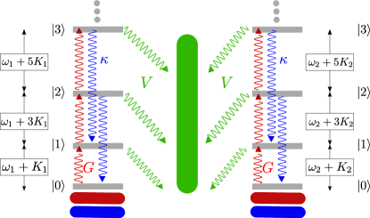
Figure 1: The four lowest-lying discrete energy levels of the quantum vdP oscillator with Kerr nonlinearity. The Kerr nonlinearity leads to an energy level spacing $\omega_{m}+(2n+1)K_{m}$ between the $n$-th and $(n+1)$-th energy levels. The wiggly lines describe non-unitary processes stemming from coupling the system to Markovian reservoirs (marked by rectangles with rounded corners): The incoherent energy gain with rate $G$ and the incoherent nonlinear energy loss with rate $\kappa$ are obtained by coupling the individual vdP oscillators to their own Markovian reservoirs. The dissipative coupling with strength $V$ is obtained by coupling the vdP oscillators to a common Markovian reservoir.

II The Model

We consider two anharmonic dissipatively coupled quantum vdP oscillators Ishibashi and Kanamoto (2017); Walter et al. (2015); Lee et al. (2014). The schematics of the energy spectrum of the oscillators and the non-unitary processes involved in the coupling to the environment are shown in Fig. 1. The time evolution of the density matrix $\rho$ of the two oscillators is governed by the quantum master equation $(\hbar=1)$

$$\partial_{t}\rho=\sum_{m=1}^{2}\left(-i[H_{m},\rho]+G\mathcal{D}[a_{m}^{\dagger}]\rho+\kappa\mathcal{D}[a_{m}^{2}]\rho\right)+V\mathcal{D}[a_{1}-a_{2}]\rho,$$ (1)

where $a_{m}$ and $a_{m}^{\dagger}$ are the annihilation and creation operators of the $m$-th oscillator, and $H_{m}=\omega_{m}a_{m}^{\dagger}a_{m}+K_{m}(a_{m}^{\dagger}a_{m})^{2}$ is the Hamiltonian of the $m$-th oscillator, with $\omega_{m}$ and $K_{m}$ being the natural frequency and the Kerr nonlinearity parameter of the $m$-th oscillator, respectively. This Hamiltonian leads to an energy level spacing $\omega_{m}+(2n+1)K_{m}$ between the $n$-th and $(n+1)$-th energy levels of the $m$-th oscillator. The non-unitary dynamics is described using Lindblad operators, $\mathcal{D}[x]\rho\equiv x\rho x^{\dagger}-(x^{\dagger}x\rho+\rho x^{\dagger}x)/2$. The parameters $G$ and $\kappa$ describe the rate of energy gain and the rate of nonlinear energy dissipation of the self-oscillators, respectively. $V$ defines the strength of the dissipative coupling. Such a dissipative coupling is obtained by assuming that the two vdP oscillators are coupled to a common Markovian reservoir Mogilevtsev et al. (2015), as schematically shown in Fig. 1. In the following, we will use QuTiP Johansson et al. (2012, 2013) to numerically simulate this master equation.

In the model described by Eq. (1), we have chosen $\kappa$ and $G$ to be identical for both vdP oscillators. This allows us to simplify our analysis by discarding any difference between the states of the two self-oscillators which may arise as a result of their individual character. This is by no means a crucial choice for observing the noise-induced amplitude death and quantum effects described below. We have maintained the freedom of choosing a non-identical natural frequency, $\omega_{m}$, as the amplitude death depends critically on the frequency detuning between the two self-oscillator. Furthermore, we allow for non-identical Kerr nonlinearity, $K_{m}$, as it helps to elucidate the quantum effects described in Sec. IV.

It is known that in the absence of a Kerr nonlinearity, the uncoupled ($V=0$) vdP oscillators exhibit limit-cycles. We would like to emphasize that this is also true in the presence of a Kerr nonlinearity. This is apparent when examining the steady state density matrix for such a Kerr nonlinear vdP oscillator, which is given by the diagonal $\rho^{(V=0)}_{nn}=(G/\kappa)^{n}\Phi(1+n,G/\kappa+n,G/\kappa)/\left[(G/\kappa)_{n}\Phi(1,G/\kappa,2G/\kappa)\right]$, where $\left(\cdot\right)_{n}$ denotes the Pochhammer symbol and $\Phi$ is Kummer’s confluent hypergeometric function Dodonov and Mizrahi (1997); Lörch et al. (2016). $\rho^{(V=0)}$ depends only on $G/\kappa$ and not on the Kerr parameter $K_{m}$. It therefore describes limit-cycles with no preferred phase, just as for the harmonic $K_{m}=0$ case.

The equations of motion for the classical amplitudes of oscillation, $\alpha_{m}\equiv\braket{a_{m}}$, can be obtained from Eq. (1). Using the Heisenberg equation of motion and after employing a mean-field approximation, one obtains

$$\partial_{t}\alpha_{m}=-i\left[\omega_{m}+2K_{m}|\alpha_{m}|^{2}\right]\alpha_{m}+\frac{G}{2}\alpha_{m}-\kappa|\alpha_{m}|^{2}\alpha_{m}+\frac{V}{2}(\alpha_{\bar{m}}-\alpha_{m}),$$ (2)

for $m\in\left\{1,2\right\}$, and where $\bar{m}\neq m$. These equations of motion constitute our classical noiseless model.

To obtain from Eq. (1) a semiclassical model, i.e. a classical model which includes Gaussian noise, we describe the system using a partial differential equation for the Wigner distribution function $W(\alpha_{1},\alpha_{1}^{*},\alpha_{2},\alpha_{2}^{*},t)$ Gardiner and Zoller (2004); Carmichael (1999); Ishibashi and Kanamoto (2017),

$$\partial_{t}W(\boldsymbol{\alpha})=\sum_{m=1}^{2} \left[-\left(\frac{\partial}{\partial\alpha_{m}}\mu_{\alpha_{m}}+\text{c.c.}\right)\right.$$ (3)

$$\left.+\frac{1}{2}\left(\frac{\partial^{2}}{\partial\alpha_{m}\partial\alpha_{m}^{*}}D_{\alpha_{m}\alpha_{m}^{*}}+\frac{\partial^{2}}{\partial\alpha_{m}\partial\alpha_{\bar{m}}^{*}}D_{\alpha_{m}\alpha_{\bar{m}}^{*}}\right)\right.$$

$$\left.+\frac{\kappa-iK_{m}}{4}\left(\frac{\partial^{3}}{\partial\alpha_{m}^{*}\partial\alpha^{2}_{m}}\alpha_{m}+\text{c.c.}\right)\right]W(\boldsymbol{\alpha}).$$

This phase-space representation is completely equivalent to the master equation description, Eq. (1). The drift coefficients are given by

$$\mu_{\alpha_{m}}= \left\{-i\left[\omega_{m}+2K_{m}|\alpha_{m}|^{2}\right]+\frac{G}{2}-\kappa\left(|\alpha_{m}|^{2}-1\right)-\frac{V}{2}\right\}\alpha_{m}$$ (4)

$$+\frac{V}{2}\alpha_{\bar{m}},$$

and the diffusion coefficients are given by

$$D_{\alpha_{m},\alpha_{m}^{*}} =G+2\kappa(2|\alpha_{m}|^{2}-1)+V,$$ (5)

$$D_{\alpha_{m},\alpha_{\bar{m}}^{*}} =-V.$$

In the classical limit ($|\alpha_{m}|\gg 1$), we can neglect the third-order derivatives of Eq. (3) Carmichael (1999); Walls and Milburn (2007). By doing so, we obtain the Fokker-Planck equation Risken (1984)

$$\partial_{t}W(\boldsymbol{\alpha})=\sum_{m=1}^{2} \left[-\left(\frac{\partial}{\partial\alpha_{m}}\mu_{\alpha_{m}}+\text{c.c.}\right)\right.$$ (6)

$$\left.+\frac{1}{2}\left(\frac{\partial^{2}}{\partial\alpha_{m}\partial\alpha_{m}^{*}}D_{\alpha_{m}\alpha_{m}^{*}}+\frac{\partial^{2}}{\partial\alpha_{m}\partial\alpha_{\bar{m}}^{*}}D_{\alpha_{m}\alpha_{\bar{m}}^{*}}\right)\right]W(\boldsymbol{\alpha}).$$

Eq. (6) constitutes our semiclassical model. It can be further transformed into an equivalent Langevin form Ishibashi and Kanamoto (2017), which can be straightforwardly numerically simulated. The transformation is shown in Appendix A.

III Noise-induced amplitude death

The rest-state of two harmonic self-oscillators is always unstable without a coupling between the two oscillators. When the two self-oscillators are dissipatively coupled, the rest-state may become stable, leading to strong amplitude suppression. This depends on the strength of the coupling $V$, and on the frequency detuning between the two self-oscillators, $\Delta\equiv\omega_{2}-\omega_{1}$. In the classical noiseless case, it is predicted that the rest-state is stable in the regime $G<V<(\Delta^{2}+G^{2})/(2G)$ Aronson et al. (1990). This behavior can be seen in Fig. 2 (a), which shows the squared amplitude $|\alpha_{1}|^{2}=|\alpha_{2}|^{2}$. For two vdP oscillators with an anharmonic energy spectrum, the effective oscillation frequency of the individual oscillators, $\tilde{\omega}_{m}\equiv\omega_{m}+2K_{m}|\alpha_{m}|^{2}$, depends on the amplitude of oscillation. This is a direct result of the anharmonicity in their energy spectrum, $K_{m}$. In the case that this anharmonicity is identical for both oscillators, $K_{1}=K_{2}=K$, the effective frequency detuning is identical to the natural frequency detuning,

$$\tilde{\Delta}=\tilde{\omega}_{2}-\tilde{\omega}_{1}=\omega_{2}-\omega_{1}+2K(|\alpha_{2}|^{2}-|\alpha_{1}|^{2})=\Delta,$$ (7)

since the relation $\alpha_{1}=\alpha_{2}$ holds in this case. We therefore expect the amplitude of oscillation of the oscillators with Kerr nonlinearity to be identical to the amplitude of oscillation of the harmonic oscillators, for any specific values of $V$ and $\Delta$. This is indeed the case, as can be seen by comparing Fig. 2 (a) with Fig. 2 (d), in which the squared amplitude of oscillation $|\alpha_{1}|^{2}=|\alpha_{2}|^{2}$ for $K/G=1$ is shown.

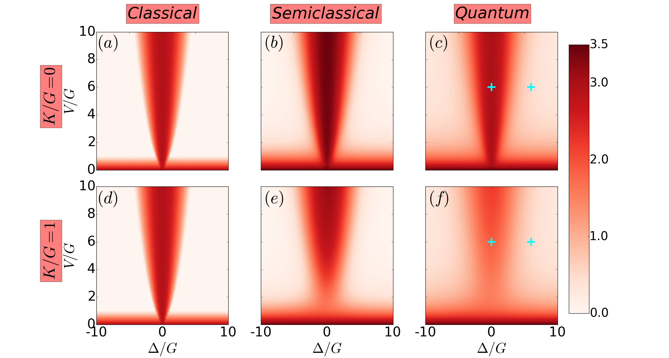
Figure 2: Amplitude suppression of two coupled self-oscillators for the harmonic and anharmonic cases in the classical, semiclassical, and quantum descriptions. (a) and (d) show the squared amplitude $|\alpha_{1}|^{2}$ of the noiseless classical oscillator obtained from Eq. (2). (b) and (e) present the long-time limit amplitude squared, $\overline{|\alpha_{1}|^{2}}$, obtained from numerically simulating the semiclassical model, Eq. (6), and then ensemble-averaging over many independent trajectories. (c) and (f) show the mean phonon number $\braket{a_{1}^{\dagger}a_{1}}$ of the quantum oscillator, Eq. (1). The upper plots (a), (b), and (c) correspond to the harmonic case, $K/G=0$. The lower plots (c), (d) and (e) correspond to the anharmonic case, with $K/G=1$. A decrease in $\overline{|\alpha_{1}|^{2}}$ and $\braket{a_{1}^{\dagger}a_{1}}$ is seen in the anharmonic case, as compared with the harmonic case. The energy loss rate is $\kappa/G=0.2$ for all plots. Cyan crosses mark the parameters for which the Wigner density functions appearing in Fig. 3 were calculated.

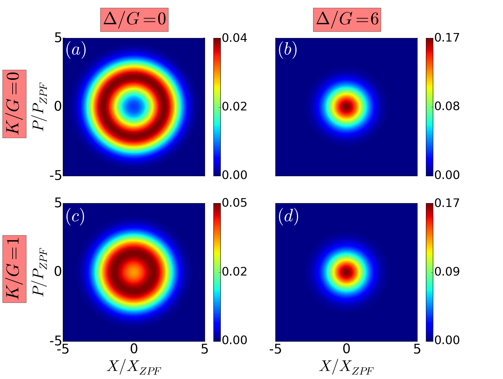
Figure 3: Wigner density function for the steady state of the oscillator before and after amplitude death occurred, for both the harmonic case and the nonlinear case. (a) and (b) correspond to the cyan crosses marked in Fig. 2 (c), while (c) and (d) match the cyan crosses shown in Fig. 2 (f). The suppression of oscillation amplitude in the presence of a Kerr nonlinearity is clearly visible by comparing (a) and (c). The limit-cycle shrinks, resulting in a decrease of $\braket{a_{1}^{\dagger}a_{1}}$. The Wigner distributions are all rotationally symmetric, having no preferred phase. In all plots, $\kappa/G=0.2$ and $V/G=6$.

For vdP oscillators in the presence of noise, on the other hand, the anharmonicity drastically changes the oscillation amplitude as compared with the harmonic case. This can be seen both in our semiclassical model, and in the fully quantum description. In Fig. 2 (b), we numerically simulate the semiclassical model, Eq. (6), for $K=0$, and show the long-time limit amplitude squared, $\overline{|\alpha_{1}|^{2}}$, which is ensemble-averaged over many independent trajectories. This $\overline{|\alpha_{1}|^{2}}$ is shown as a function of both the detuning $\Delta$ and the coupling strength $V$. Oscillations are sustained for small enough $\Delta$, with slightly higher amplitudes than in the noiseless case. This oscillation amplitude is highly suppressed in the regime where amplitude death is expected. Nevertheless, the amplitude of oscillation does not vanish completely, as noise hinders the complete collapse. This agrees with Ref. Ishibashi and Kanamoto (2017). In Fig. 2 (e), in which $\overline{|\alpha_{1}|^{2}}$ is shown for $K/G=1$, and in contrast to the classical noiseless case, the amplitudes of oscillation are significantly changed. This can be seen by comparing Fig. 2 (e) to Fig. 2 (b). It is seen that the values of $\overline{|\alpha_{1}|^{2}}$ for $V>G$ are significantly lower for the anharmonic case, as compared with the harmonic case.

As mentioned, a similar decrease is seen also in the quantum description. In Fig. 2 (c) we show the mean phonon number of the first oscillator $\braket{a^{\dagger}_{1}a_{1}}$ for the harmonic case, as a function of $\Delta$ and $V$. As discussed in Ref. Ishibashi and Kanamoto (2017), the mean phonon number significantly decreases in the regime where amplitude death is expected classically, but does not vanish completely. Noise prevents the complete collapse. This can also be seen in Fig. 3 (a) and Fig. 3 (b), in which we plot the Wigner function representation of the steady state of the oscillator before and after amplitude death occurred. The parameters chosen for these Wigner representations are marked in cyan crosses in Fig. 2 (c). After amplitude death takes place, the probability distribution is sharply concentrated about the axis origin, leading to low phonon expectation values $\braket{a_{1}^{\dagger}a_{1}}$. When nonlinearity is introduced, just as in the semiclassical description, the mean phonon number of the oscillators is significantly changed. This is seen in Fig. 2 (f), in which the mean phonon number $\braket{a^{\dagger}_{1}a_{1}}$ is shown for $K/G=1$. As in the semiclassical description, it is seen that the values of $\braket{a^{\dagger}_{1}a_{1}}$ for $V>G$ are significantly lower for the $K/G=1$ case, as compared with the $K/G=0$ case. This is also seen in the Wigner function representation, shown for the nonlinear case in Fig. 3 (c) and in Fig. 3 (d), for the parameters marked in cyan crosses in Fig. 2 (f). Even before amplitude death occurred, the limit-cycle of the oscillator shrank as compared with the harmonic case, Fig. 3 (a). The nonlinearity leads therefore to a decrease of $\braket{a_{1}^{\dagger}a_{1}}$ in the quantum case. Note that while Fig. 2 and Fig. 3 show the average phonon number and Wigner function representation of the first oscillator, almost identical figures are obtained for the second oscillator (see Fig. 6 (d) and discussion in the end of Sec. IV).

The underlying cause for this decrease, seen in the semiclassical model and in the quantum description, is noise. When noise is present, the amplitude of the self-oscillator fluctuates, as is implied by the existence of a diffusion constant, Eq. (5). The effective frequency of the oscillators with Kerr nonlinearity, $\tilde{\omega}_{m}$, depends on this fluctuating amplitude of oscillation. For that reason, the frequency is now a fluctuating quantity as well. The bigger the anharmonicity $K$ is, the larger the frequency fluctuations become. This implies that when noise is present in the system, the spread of values for $\tilde{\Delta}$ is wider than the spread of values of the effective detuning for harmonic self-oscillators, $\Delta$. Therefore, increasing $K$ has a similar effect as increasing the effective detuning between the two self-oscillators. As the dissipative coupling is sensitive to the detuning, we see the effect of increasing $K$ as a decrease in $\braket{a_{1}^{\dagger}a_{1}}$ ($\braket{a_{2}^{\dagger}a_{2}}$) , for $V>G$. For $V\ll G$, on the other hand, the dissipative term plays only a minor role. Therefore, increasing $K$ does not significantly change the occupation number $\braket{a_{1}^{\dagger}a_{1}}$ ($\braket{a_{2}^{\dagger}a_{2}}$).

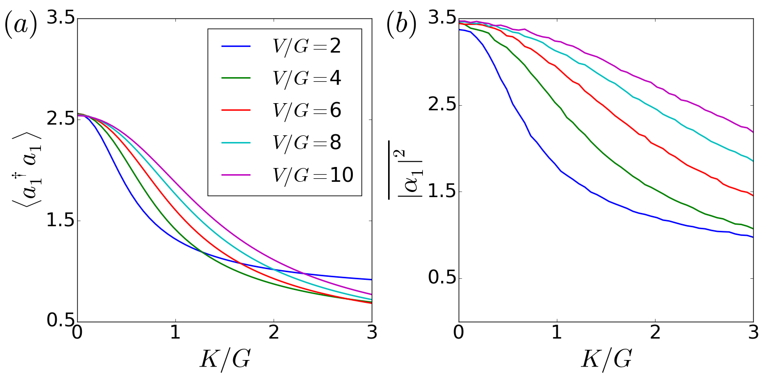
Figure 4: (a) Average occupation number, $\braket{a_{1}^{\dagger}a_{1}}$, as a function of $K$. It is obtained using Eq. (1). (b) Average oscillation amplitude squared obtained from Eq. (6), $\overline{|\alpha_{1}|^{2}}$, as a function of $K$. In both noisy models, a noticeable decrease in the oscillation amplitude is seen for increasing $K$. The legend shown describes both plots. Other parameters used in both plots are $(\kappa,\Delta)=(0.2,0.0)\times G$.

In Fig. 4 (a), we numerically simulate the quantum master equation, Eq. (1), and show the decrease of $\braket{a^{\dagger}_{1}a_{1}}$ for increasing $K$. In Fig. 4 (b), we numerically simulate the semiclassical model, Eq. (6), and show the decrease in the average amplitude squared, $\overline{|\alpha_{1}|^{2}}$, for increasing $K$. Indeed, both noisy models show this decrease, and only quantitative differences can be seen when comparing the two. The noiseless classical model cannot account for this amplitude suppression, as is seen in Fig. 2. We therefore conclude that this amplitude suppression, or average occupation number reduction, is noise-induced.

For very large values of $K/G$, this noise-induced amplitude suppression can balance the amplitude growth induced by the linear energy gain $G$. This allows us to set $\kappa=0$ for these cases, while still keeping the self-oscillators in the quantum parameter regime in which only a small number of energy levels is populated (see Sec. IV). For smaller values of $K/G$, a finite $\kappa$ is required to keep the oscillators in the quantum parameter regime.

IV Quantum effects - Amplitude revival

In the quantum parameter regime, the anharmonicity leads to genuine quantum effects in the amplitude death phenomenon, which cannot be modeled using a semiclassical model. They are the result of the quantized, discrete energy spectrum of the oscillators (see Fig. 1). The Kerr anharmonicity $K_{m}$ leads to an energy level spacing $\omega_{m}+(2n+1)K_{m}$ between the $n$-th and the $(n+1)$-th Fock levels of the $m$-th anharmonic quantum vdP oscillator. There are therefore several discrete frequencies relevant for each oscillator. As the amplitude death phenomenon depends on the detuning between the frequencies of the oscillators, we can expect this discreteness to be reflected in the mean phonon number $\braket{a_{m}^{\dagger}a_{m}}$ of each oscillator. In order to observe this discreteness however, one must also consider the broadening of the energy levels due to the dissipative processes. Working in a parameter regime in which the energy level spacing is much larger than the energy level broadening is therefore a necessity.

To see an example of this, consider one quantum anharmonic vdP oscillator to have a Kerr nonlinearity $K_{1}$, while the second vdP oscillator is harmonic, i.e. $K_{2}=0$. Deep in the quantum parameter regime, in which only the lowest three energy levels of each oscillator are populated, just three frequencies are relevant: The transition frequencies between the populated energy levels of the first oscillator, $\omega_{1}+K_{1}$ and $\omega_{1}+3K_{1}$, and the frequency of the second oscillator, $\omega_{2}$. The effective detuning between the two oscillators could therefore be minimized at two discrete values, $\tilde{\Delta}=\omega_{2}-\omega_{1}-K_{1}=0$ and $\tilde{\Delta}=\omega_{2}-\omega_{1}-3K_{1}=0$. At these values for which the effective detuning is minimized, we expect to see a revival of the oscillation amplitude. In Fig. 5 (a), the blue curve depicts $\braket{a_{1}^{\dagger}a_{1}}=\braket{a_{2}^{\dagger}a_{2}}$ obtained by numerically simulating the master equation, Eq. (1), for the example just described (the Fock level probability distribution is shown in the left inset). The peaks in the mean phonon number are clearly visible. The red curve in Fig. 5 (a) depicts the peaks in $\braket{a_{1}^{\dagger}a_{1}}=\braket{a_{2}^{\dagger}a_{2}}$ for a smaller $V$, i.e. for a parameter regime in which more Fock levels are populated (see right inset). Indeed, the peaks are seen in this case for $\Delta=(2n+1)K_{1}$, with $n$ being a nonnegative integer. The average oscillation amplitude squared, $\overline{|\alpha_{1}|^{2}}=\overline{|\alpha_{2}|^{2}}$, predicted by the semiclassical model, is shown in Fig. 5 (b). As in Fig. 5 (a), the blue and red curve correspond to $V/G=8$ and $V/G=2$, respectively. In both cases, only one peak is seen. This is expected, as the energy distribution is continuous in the semiclassical case. One can furthermore observe a mismatch in the peak location between the two cases. This is a classical effect, caused by the fact that the frequency of the nonlinear oscillator depends on the amplitude of oscillation, $\tilde{\omega}_{1}=\omega_{1}+2K_{1}|\alpha_{1}|^{2}$. The peak appears for $\omega_{2}=\tilde{\omega}_{1}$, i.e. for $\Delta=2K_{1}|\alpha_{1}|^{2}$. Smaller values of $V$ correspond to a larger amplitude of oscillation, and therefore the peak for $V/G=2$ appears to the right of the peak for $V/G=8$.

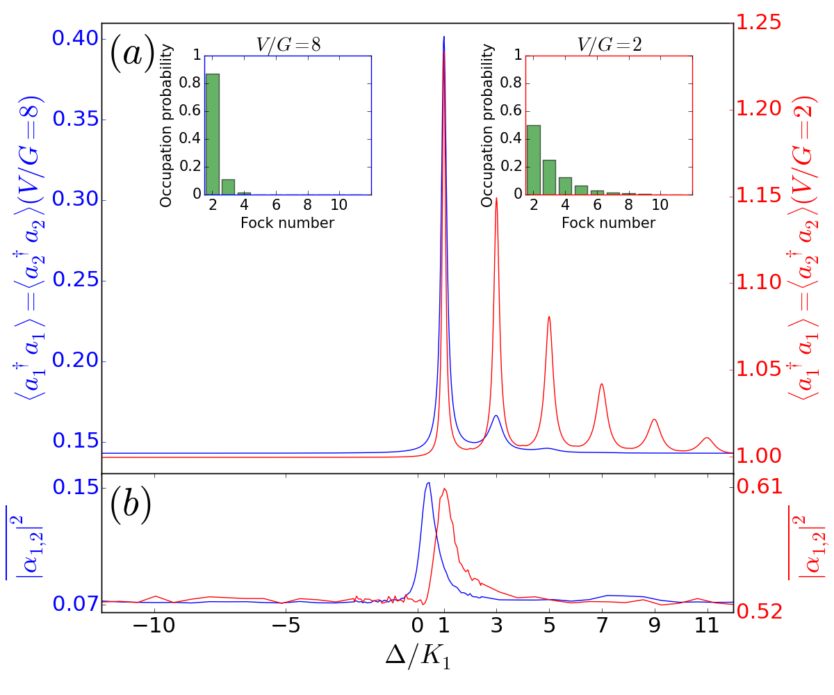
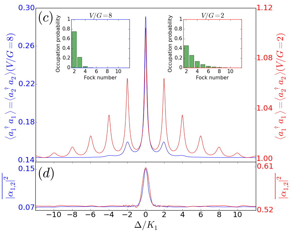
Figure 5: Average occupation number $\braket{a_{1}^{\dagger}a_{1}}=\braket{a_{2}^{\dagger}a_{2}}$ and average oscillation amplitude squared $\overline{|\alpha_{1}|^{2}}=\overline{|\alpha_{2}|^{2}}$, obtained from Eq. (1) and Eq. (6) respectively, are shown as a function of the detuning in (a) and (b) for a vdP oscillator with very strong nonlinearity $K_{1}/G=50$ coupled to a harmonic ($K_{2}/G=0$) vdP oscillator. In (c) and (d), the same quantities are shown for two anharmonic ($K_{1}/G=K_{2}/G=50$) coupled vdP oscillators. In all plots, blue curves correspond to $V/G=8$, while red curves correspond to $V/G=2$. The Fock basis probability distributions for both these coupling strengths are shown in the insets (calculated for $\Delta=0$). The individual dissipation rate is $\kappa/G=0$.

We now also consider the case in which both the vdP oscillators have an anharmonic energy spectrum. An example is shown in Fig. 5 (c), in which the occupation number $\braket{a_{1}^{\dagger}a_{1}}=\braket{a_{2}^{\dagger}a_{2}}$ of both oscillators is plotted as a function of the detuning $\Delta$, for equal Kerr nonlinearities $K_{1}=K_{2}\equiv K$. The blue curve corresponds to strong dissipative coupling $V$ for which only the first three low-lying Fock levels are populated (left inset), while the red curve corresponds to smaller $V$, for which more Fock levels have non-negligible population (right inset). We now expect phonon number peaks for $\Delta=2nK$, with $n$ being an integer. These correspond to resonances between the transition frequencies of the two anharmonic oscillators, for the non-negligibly populated Fock states. The blue and red curve shown in Fig. 5 (d) present the single peak which is predicted by the semiclassical model. Contrary to Fig. 5 (b), and because both oscillators are nonlinear with $K_{1}=K_{2}$, both peaks appear at the same detuning $\Delta=0$.

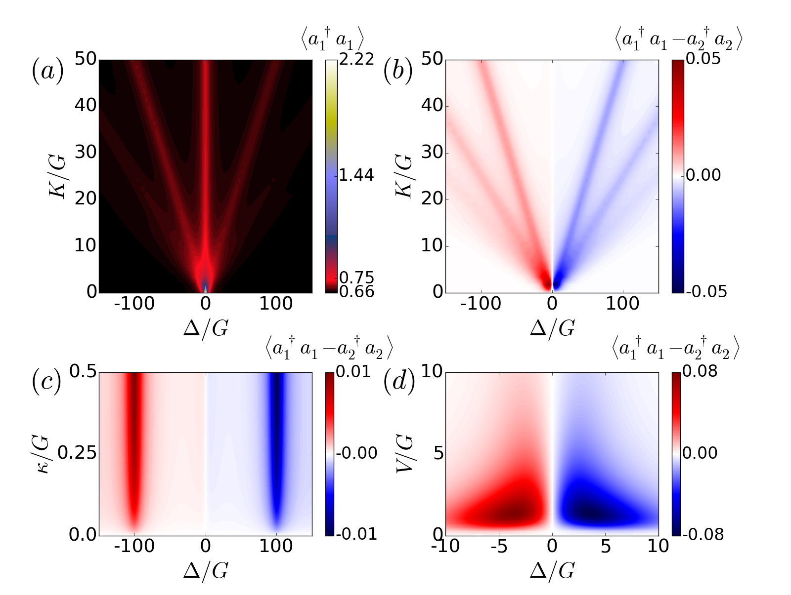
Figure 6: (a) Average occupation number $\braket{a_{1}^{\dagger}a_{1}}$ as a function of $\Delta$ and $K$. Peaks in the occupation number at $K=\pm 2\Delta$ are clearly visible. (b) Difference in occupation number between the two oscillators, $\braket{a_{1}^{\dagger}a_{1}-a_{2}^{\dagger}a_{2}}$. The oscillation revival is more apparent in the $m$-th oscillator, if it involves its lowest frequency $\omega_{m}+K$. Other parameters are $(\kappa,V)/G=(0.25,2)$ in both plots. (c) Average occupation number difference, $\braket{a_{1}^{\dagger}a_{1}-a_{2}^{\dagger}a_{2}}$, as a function of $\Delta$ and $\kappa$. Other parameters are $(K,V)/G=(50,2)$. The difference becomes more pronounced as $\kappa$ is increased. (d) $\braket{a_{1}^{\dagger}a_{1}-a_{2}^{\dagger}a_{2}}$ for parameters corresponding to Fig. 2 (f), $(K,\kappa)/G=(1,0.2)$.

In the previously described examples, we set $\kappa/G=0$. The energy gain $G$ was balanced by the dissipative coupling $V$. This was possible because we have used large Kerr parameters $K_{1}$ or $K_{2}$, which therefore, as explained in Sec. III, made the dissipative coupling more effective. For small values of $K_{1}$ and $K_{2}$, a finite value of $\kappa$ needs to be introduced in order to keep the system in the quantum parameter regime.

Figure 6(a) illustrates that in the absence of Kerr anharmonicity, i.e. $K_{1}=K_{2}\equiv K=0$, the two oscillators have a high phonon number only for $\Delta=0$. As $|\Delta|$ is increased, the oscillation-amplitude is strongly suppressed. For larger values of $K$, the oscillation amplitudes becomes much smaller, as the dissipative coupling is more effective. Still, for $\Delta=0$, we have a peak in the phonon number. As we increase $|\Delta|$, the phonon number decreases. But once $|\Delta|$ gets closer to the resonance condition $|\Delta|=2K$, the phonon number increases again.

In Fig. 6 (a), a dissipation rate of $\kappa/G=0.25$ was chosen. It is needed to balance the energy gain $G$ for the lower values of $K$. This value of $\kappa$ introduces a small asymmetry between negative and positive detuning $\Delta$. In Fig. 6 (b) the difference of the phonon number between the two oscillators, $\braket{a_{1}^{\dagger}a_{1}-a_{2}^{\dagger}a_{2}}$, is shown. We can see that for negative detunings, the phonon number peaks are more pronounced for oscillator 1. For positive detunings, the opposite is true. To understand this effect, we need to consider the frequency resonances relevant to a corresponding phonon number peak. For $\Delta>0$ ($\Delta<0$) and $K>0$, the resonances involve the lowest possible transition frequency of the second (first) oscillator, with higher transition frequencies of the first (second) oscillator. As $\kappa$ is influencing energy levels higher than the ground state, its effect is less detrimental on the oscillator for which the lowest possible frequency is relevant. We therefore expect that if the relations $K>0$ and $\kappa>0$ hold, such an asymmetry occurs. In Fig. 6 (c), the difference $\braket{a_{1}^{\dagger}a_{1}-a_{2}^{\dagger}a_{2}}$ is plotted as a function of the detuning $\Delta$ and of $\kappa$ (other parameters are (V, K)/G=(2, 50)). It is indeed seen that $\braket{a_{1}^{\dagger}a_{1}-a_{2}^{\dagger}a_{2}}=0$ for $\kappa=0$. As $\kappa$ is in increasing, so is the difference $\braket{a_{1}^{\dagger}a_{1}-a_{2}^{\dagger}a_{2}}$. In Fig. 6 (d) we show the difference $\braket{a_{1}^{\dagger}a_{1}-a_{2}^{\dagger}a_{2}}$ for parameters corresponding to Fig. 2 (f).

V Conclusions

In this paper, we have studied theoretically the amplitude death phenomenon for two coupled anharmonic quantum vdP oscillators. We have shown that the anharmonicity leads to smaller oscillation amplitudes in semiclassical model and in the quantum description, an effect which we have shown to be the result of noise. Furthermore, we have found in the quantum description qualitative differences as compared with the semiclassical model. Peaks in the mean phonon number of the oscillators are seen as a function of their detuning. They describe quantized amplitude death, and then oscillation revival. We have shown that these peaks correspond to discrete transition frequencies in the energy spectrum of the anharmonic vdP oscillators, and that they are therefore not seen in a semiclassical model. To the best of our knowledge, this is the first time genuine quantum effects are discussed in the context of the amplitude death phenomenon.

Quantum vdP oscillators with a dissipative coupling can be engineered in a variety of systems. In trapped ion systems, one-phonon gain and two-phonon loss can be implemented using appropriately red- and blue-detuned drives Lee and Sadeghpour (2013). The dissipative coupling can be implemented using various techniques Lee et al. (2014); Schindler et al. (2013); Diehl et al. (2008). For these systems, large Kerr nonlinearities $K_{1}$ and $K_{2}$ can be engineered Lörch et al. (2017); Zhao and Babikov (2008); Wang and Babikov (2011); Home et al. (2011). In cavity optomechanical systems, quantum vdP oscillators can be realized using “membrane-in-the-middle” setups Walter et al. (2014); Thompson et al. (2008). The two-phonon loss is obtained by placing the membrane at a node of the cavity field, and then driving the cavity with an appropriate red-detuned drive. The one-phonon gain is implemented via a coupling to another cavity mode, which is driven by an appropriate blue-detuned laser. A dissipative coupling of the form $\mathcal{D}[a_{m}-a_{\bar{m}}]$ between two such quantum vdP oscillators can be implemented using an additional cavity Walter et al. (2014). Engineering large Kerr nonlinearities in optomechanical systems is extremely challenging and has not been demonstrated, but hybrid systems such as Rips et al. (2014); Rimberg et al. (2014) exploiting strong nonlinearities from auxiliary systems have been proposed. Realizing this experiment will demonstrate a new quantum effect in the amplitude dynamics of non-linear coupled oscillators.

Appendix A Transforming the Fokker-Planck equation to a Langevin equation

Following Ref. Ishibashi and Kanamoto (2017), we first rewrite the Fokker-Planck equation, Eq. (6), to Cartesian coordinates. Using $\alpha_{m}=x_{m}+iy_{m}$, we find

$$\partial_{t}W(\boldsymbol{X}) =\sum_{m=1}^{2}\left[-\left(\frac{\partial}{\partial x_{m}}\mu_{x_{m}}+\frac{\partial}{\partial y_{m}}\mu_{y_{m}}\right)+\frac{1}{2}\left(\frac{\partial^{2}}{\partial x^{2}_{m}}D_{x_{m}x_{m}}\right.\right.$$ (8)

$$\left.\left.+\frac{\partial^{2}}{\partial y^{2}_{m}}D_{y_{m}y_{m}}+\frac{\partial^{2}}{\partial x_{m}\partial x_{\bar{m}}}D_{x_{m}x_{\bar{m}}}+\frac{\partial^{2}}{\partial y_{m}\partial y_{\bar{m}}}D_{y_{m}y_{\bar{m}}}\right)\right]W(\boldsymbol{X}),$$

where $\boldsymbol{X}=(x_{1},y_{1},x_{2},y_{2})$, the drift vector $\boldsymbol{\mu}=(\mu_{x_{1}},\mu_{y_{1}},\mu_{x_{2}},\mu_{y_{2}})$ is given by

$$\mu_{x_{m}}= \left[\omega_{m}+2K_{m}(x_{m}^{2}+y_{m}^{2})\right]y_{m}$$ (9)

$$+\left[\frac{G}{2}-\kappa(x_{m}^{2}+y_{m}^{2}-1)-\frac{V}{2}\right]x_{m}+\frac{V}{2}x_{\bar{m}},$$

$$\mu_{y_{m}}= -\left[\omega_{m}+2K_{m}(x_{m}^{2}+y_{m}^{2})\right]x_{m}$$ (10)

$$+\left[\frac{G}{2}-\kappa(x_{m}^{2}+y_{m}^{2}-1)-\frac{V}{2}\right]y_{m}+\frac{V}{2}y_{\bar{m}},$$

and the diffusion matrix is given by

$$\boldsymbol{D}=\frac{1}{2}\left[\begin{array}[]{cccc}\nu_{1}&0&-V/2&0\\ 0&\nu_{1}&0&-V/2\\ -V/2&0&\nu_{2}&0\\ 0&-V/2&0&\nu_{2}\end{array}\right],$$ (11)

where $\nu_{m}=G/2+\kappa\left[2(x_{m}^{2}+y_{m}^{2})-1\right]+V/2$.

The Langevin equation corresponding to Eq. (8) is

$$\mathrm{d}\boldsymbol{X}=\boldsymbol{\mu}\mathrm{d}t+\boldsymbol{\sigma}\mathrm{d}\boldsymbol{W}_{t},$$ (12)

where $\mathrm{d}\boldsymbol{W}_{t}$ is the Wiener increment, and the noise strength is obtained via $\boldsymbol{\sigma}=\boldsymbol{U}\sqrt{\boldsymbol{D}^{\prime}}\boldsymbol{U}^{-1}$, where $\boldsymbol{D}^{\prime}=\boldsymbol{U}^{-1}\boldsymbol{D}\boldsymbol{U}$ is the diagonalized form of $\boldsymbol{D}$. As the Kerr nonlinearity does not appear in the diffusion matrix, the analytical derivation and exact expression for the noise term is identical to what is shown in Ref. Ishibashi and Kanamoto (2017).

References

- Pikovsky et al. (2003) A. Pikovsky, M. Rosenblum, and J. Kurths, Synchronization: A Universal Concept in Nonlinear Sciences (Cambridge University Press, 2003).
- Balanov et al. (2009) A. Balanov, N. Janson, D. Postnov, and O. Sosnovtseva, Synchronization: from simple to complex (Springer, 2009).
- Lee and Sadeghpour (2013) T. E. Lee and H. R. Sadeghpour, Phys. Rev. Lett. 111, 234101 (2013).
- Walter et al. (2014) S. Walter, A. Nunnenkamp, and C. Bruder, Phys. Rev. Lett. 112, 094102 (2014).
- Weiss et al. (2017) T. Weiss, S. Walter, and F. Marquardt, Phys. Rev. A 95, 041802 (2017).
- Lee et al. (2014) T. E. Lee, C.-K. Chan, and S. Wang, Phys. Rev. E 89, 022913 (2014).
- Walter et al. (2015) S. Walter, A. Nunnenkamp, and C. Bruder, Annalen der Physik 527, 131 (2015).
- Ameri et al. (2015) V. Ameri, M. Eghbali-Arani, A. Mari, A. Farace, F. Kheirandish, V. Giovannetti, and R. Fazio, Phys. Rev. A 91, 012301 (2015).
- Bastidas et al. (2015) V. M. Bastidas, I. Omelchenko, A. Zakharova, E. Schöll, and T. Brandes, Phys. Rev. E 92, 062924 (2015).
- Lörch et al. (2016) N. Lörch, E. Amitai, A. Nunnenkamp, and C. Bruder, Phys. Rev. Lett. 117, 073601 (2016).
- Sonar et al. (2018) S. Sonar, M. Hajdušek, M. Mukherjee, R. Fazio, V. Vedral, S. Vinjanampathy, and L.-C. Kwek, Phys. Rev. Lett. 120, 163601 (2018).
- Amitai et al. (2017) E. Amitai, N. Lörch, A. Nunnenkamp, S. Walter, and C. Bruder, Phys. Rev. A 95, 053858 (2017).
- Lörch et al. (2017) N. Lörch, S. E. Nigg, A. Nunnenkamp, R. P. Tiwari, and C. Bruder, Phys. Rev. Lett. 118, 243602 (2017).
- Xu et al. (2014) M. Xu, D. A. Tieri, E. C. Fine, J. K. Thompson, and M. J. Holland, Phys. Rev. Lett. 113, 154101 (2014).
- Weiss et al. (2016) T. Weiss, A. Kronwald, and F. Marquardt, New Journal of Physics 18, 013043 (2016).
- Ishibashi and Kanamoto (2017) K. Ishibashi and R. Kanamoto, Phys. Rev. E 96, 052210 (2017).
- Aronson et al. (1990) D. G. Aronson, G. B. Ermentrout, and N. Kopell, Physica D: Nonlinear Phenomena 41, 403 (1990).
- Ermentrout (1990) G. Ermentrout, Physica D: Nonlinear Phenomena 41, 219 (1990).
- Mirollo and Strogatz (1990) R. E. Mirollo and S. H. Strogatz, Journal of Statistical Physics 60, 245 (1990).
- Saxena et al. (2012) G. Saxena, A. Prasad, and R. Ramaswamy, Physics Reports 521, 205 (2012).
- Koseska et al. (2013a) A. Koseska, E. Volkov, and J. Kurths, Phys. Rev. Lett. 111, 024103 (2013a).
- Koseska et al. (2013b) A. Koseska, E. Volkov, and J. Kurths, Physics Reports 531, 173 (2013b).
- Mogilevtsev et al. (2015) D. Mogilevtsev, G. Y. Slepyan, E. Garusov, S. Y. Kilin, and N. Korolkova, New Journal of Physics 17, 043065 (2015).
- Johansson et al. (2012) J. Johansson, P. Nation, and F. Nori, Computer Physics Communications 183, 1760 (2012).
- Johansson et al. (2013) J. Johansson, P. Nation, and F. Nori, Computer Physics Communications 184, 1234 (2013).
- Dodonov and Mizrahi (1997) V. V. Dodonov and S. S. Mizrahi, J. Phys. A. Math. Gen. 30, 5657 (1997).
- Gardiner and Zoller (2004) C. Gardiner and P. Zoller, Quantum Noise: A Handbook of Markovian and Non-Markovian Quantum Stochastic Methods with Applications to Quantum Optics (Springer, 2004), 3rd ed.
- Carmichael (1999) H. Carmichael, Statistical Methods in Quantum Optics 1: Master Equations and Fokker-Planck Equations (Springer, 1999).
- Walls and Milburn (2007) D. F. Walls and G. J. Milburn, Quantum Optics (Springer, 2007).
- Risken (1984) H. Risken, The Fokker-Planck Equation (Springer, 1984).
- Schindler et al. (2013) P. Schindler, M. Müller, D. Nigg, J. T. Barreiro, E. A. Martinez, M. Hennrich, T. Monz, S. Diehl, P. Zoller, and R. Blatt, Nature Physics 9, 361 (2013).
- Diehl et al. (2008) S. Diehl, A. Micheli, A. Kantian, B. Kraus, H. P. Büchler, and P. Zoller, Nature Physics 4, 878 (2008).
- Zhao and Babikov (2008) M. Zhao and D. Babikov, Phys. Rev. A 77, 012338 (2008).
- Wang and Babikov (2011) L. Wang and D. Babikov, Phys. Rev. A 83, 022305 (2011).
- Home et al. (2011) J. P. Home, D. Hanneke, J. D. Jost, D. Leibfried, and D. J. Wineland, New Journal of Physics 13, 073026 (2011).
- Thompson et al. (2008) J. D. Thompson, B. M. Zwickl, A. M. Jayich, F. Marquardt, S. M. Girvin, and J. G. E. Harris, Nature 452, 72 (2008).
- Rips et al. (2014) S. Rips, I. Wilson-Rae, and M. J. Hartmann, Phys. Rev. A 89, 013854 (2014).
- Rimberg et al. (2014) A. J. Rimberg, M. P. Blencowe, A. D. Armour, and P. D. Nation, New Journal of Physics 16, 055008 (2014).