A probabilistic framework for multi-view feature learning
with many-to-many associations via neural networks

Abstract

A simple framework Probabilistic Multi-view Graph Embedding (PMvGE) is proposed for multi-view feature learning with many-to-many associations so that it generalizes various existing multi-view methods. PMvGE is a probabilistic model for predicting new associations via graph embedding of the nodes of data vectors with links of their associations. Multi-view data vectors with many-to-many associations are transformed by neural networks to feature vectors in a shared space, and the probability of new association between two data vectors is modeled by the inner product of their feature vectors. While existing multi-view feature learning techniques can treat only either of many-to-many association or non-linear transformation, PMvGE can treat both simultaneously. By combining Mercer’s theorem and the universal approximation theorem, we prove that PMvGE learns a wide class of similarity measures across views. Our likelihood-based estimator enables efficient computation of non-linear transformations of data vectors in large-scale datasets by minibatch SGD, and numerical experiments illustrate that PMvGE outperforms existing multi-view methods.

Table 1: Comparison of PMvGE with existing multi-view / graph-embedding methods. (Nv): Number of views, (MM): Many-to-many, (NL): Non-linear, (Ind): Inductive, (Lik): Likelihood-based. PMvGE has all the properties. $\text{Nv}=D$ represents that the method can deal with arbitrary number of views.

	(Nv)	(MM)	(NL)	(Ind)	(Lik)
CCA	2			✓
DCCA	2		✓	✓
MCCA	$D$			✓
SGE	0	✓
LINE	0	✓			✓
LPP	1	✓		✓
CvGE	2	✓		✓
CDMCA	$D$	✓		✓
DeepWalk	0	✓			✓
SBM	1	✓		✓	✓
GCN	1	✓	✓		✓
GraphSAGE	1	✓	✓	✓	✓
IDW	1	✓	✓	✓	✓
PMvGE	$D$	✓	✓	✓	✓

1 Introduction

With the rapid development of Internet communication tools in past few decades, many different types of data vectors become easily obtainable these days, advancing the development of multi-view data analysis methods (Sun,, 2013; Zhao et al.,, 2017). Different types of vectors are called as “views”, and their dimensions may be different depending on the view. Typical examples are data vectors of images, text tags, and user attributes available in Social Networking Services (SNS). However, we cannot apply standard data analysis methods, such as clustering, to multi-view data vectors, because data vectors from different views, say, images and text tags, are not directly compared with each other. In this paper, we work on multi-view Feature Learning for transforming the data vectors from all the views into new vector representations called “feature vectors” in a shared euclidean subspace.

One of the best known approaches to multi-view feature learning is Canonical Correlation Analysis (Hotelling,, 1936, CCA) for two-views, and Multiset CCA (Kettenring,, 1971, MCCA) for many views. CCA considers pairs of related data vectors $\{(\boldsymbol{x}^{(1)}_{i},\boldsymbol{x}^{(2)}_{i})\}_{i=1}^{n}\subset\mathbb{R}^{p_{1}}\times\mathbb{R}^{p_{2}}$. For instance, $\boldsymbol{x}^{(1)}_{i}\in\mathbb{R}^{p_{1}}$ may represent an image, and $\boldsymbol{x}^{(2)}_{i}\in\mathbb{R}^{p_{2}}$ may represent a text tag. Their dimension $p_{1}$ and $p_{2}$ may be different. CCA finds linear transformation matrices $\boldsymbol{A}^{(1)},\boldsymbol{A}^{(2)}$ so that the sum of inner products $\sum_{i=1}^{n}\langle\boldsymbol{A}^{(1)\top}\boldsymbol{x}^{(1)}_{i},\boldsymbol{A}^{(2)\top}\boldsymbol{x}^{2}_{i}\rangle$ is maximized under a variance constraint. The obtained linear transformations compute feature vectors $\boldsymbol{y}^{(1)}_{i}:=\boldsymbol{A}^{(1)\top}\boldsymbol{x}^{(1)}_{i},\boldsymbol{y}^{(2)}_{i}:=\boldsymbol{A}^{(2)\top}\boldsymbol{x}^{(2)}_{i}\in\mathbb{R}^{K}$ where $K\leq\min\{p_{1},p_{2}\}$ is the dimension of the shared space of feature vectors from the two views. However, the linear transformations may not capture the underlying structure of real-world datasets due to its simplicity.

To enhance the expressiveness of transformations, CCA has been further extended to non-linear settings, as Kernel CCA (Lai and Fyfe,, 2000) and Deep CCA (Andrew et al.,, 2013; Wang et al.,, 2016, DCCA) which incorporate kernel methods and neural networks to CCA, respectively. These methods show drastic improvements in performance in face recognition (Zheng et al.,, 2006) and image-text embedding (Yan and Mikolajczyk,, 2015). However, these CCA-based approaches are limited to multi-view data vectors with one-to-one correspondence across views.

Real-world datasets often have more complex association structures among the data vectors, thus the whole dataset is interpreted as a large graph with nodes of data vectors and links of the associations. For example, associations between images $\{\boldsymbol{x}^{(1)}_{i}\}_{i=1}^{n_{1}}$ and their tags $\{\boldsymbol{x}^{(2)}_{j}\}_{j=1}^{n_{2}}$ may be many-to-many relationships, in the sense that each image has multiple associated tags as well as each tag has multiple associated images. The weight $w_{ij}\geq 0$, which we call “link weight”, is defined to represent the strength of association between data vectors $\boldsymbol{x}^{(1)}_{i},\boldsymbol{x}^{(2)}_{j}$ ($i=1,2,\ldots,n_{1};j=1,2,\ldots,n_{2}$). The number of data vectors $n_{1},n_{2}$ in each view may be different.

To fully utilize the complex associations represented by $\{w_{ij}\}$, Cross-view Graph Embedding (Huang et al.,, 2012, CvGE) and its extension to more than three views called Cross-Domain Matching Correlation Analysis (Shimodaira,, 2016, CDMCA) are proposed recently, by extending CCA to many-to-many settings. 2-view CDMCA ($=\,$CvGE) obtains linear transformation matrices $\boldsymbol{A}^{(1)},\boldsymbol{A}^{(2)}$ so that the sum of inner products $\sum_{i=1}^{n_{1}}\sum_{j=1}^{n_{2}}w_{ij}\langle\boldsymbol{A}^{(1)\top}\boldsymbol{x}^{(1)}_{i},\boldsymbol{A}^{(2)\top}\boldsymbol{x}^{(2)}_{j}\rangle$ is maximized under a variance constraint.

CDMCA includes various existing multi-view / graph-embedding methods as special cases. For instance, 2-view CDMCA obviously includes CCA as a special case $w_{ij}=\delta_{ij}$, where $\delta_{ij}$ is Kronecker’s delta. By considering $1$-view setting, where $\boldsymbol{x}_{i}\in\mathbb{R}^{p}$ is a 1-view data vector and $w_{ij}\geq 0$ is a link weight between $\boldsymbol{x}_{i}$ and $\boldsymbol{x}_{j}$, CDMCA reduces to Locality Preserving Projections (He and Niyogi,, 2004; Yan et al.,, 2007, LPP). LPP also reduces to Spectral Graph Embedding (Chung,, 1997; Belkin and Niyogi,, 2001, SGE), which is interpreted as “0-view” graph embedding, by letting $\boldsymbol{x}_{i}\in\{0,1\}^{n}$ be 1-hot vector with 1 at $i$-th entry and 0 otherwise.

Although CDMCA shows a good performance in word and image embeddings (Oshikiri et al.,, 2016; Fukui et al.,, 2016), its expressiveness is still limited due to its linearity. There has been a necessity of a framework, which can deal with many-to-many associations and non-linear transformations simultaneously. Therefore, in this paper, we propose a non-linear framework for multi-view feature learning with many-to-many associations. We name the framework as Probabilistic Multi-view Graph Embedding (PMvGE). Since PMvGE generalizes CDMCA to non-linear setting, PMvGE can be regarded as a generalization of various existing multi-view methods as well.

PMvGE is built on a simple observation: many existing approaches to feature learning consider the inner product similarity of feature vectors. For instance, the objective function of CDMCA is the weighted sum of the inner product $\langle\boldsymbol{y}_{i},\boldsymbol{y}_{j}\rangle$ of the two feature vectors $\boldsymbol{y}_{i}$ and $\boldsymbol{y}_{j}$ in the shared space. Turning our eyes to recent $1$-view feature learning, Graph Convolutional Network (Kipf and Welling,, 2017), GraphSAGE (Hamilton et al.,, 2017), and Inductive DeepWalk (Dai et al.,, 2018) assume that the inner product of feature vectors $\langle\boldsymbol{y}_{i},\boldsymbol{y}_{j}\rangle$ approximates link weight $w_{ij}\geq 0$.

Inspired by these existing studies, for $D$-view feature learning ($D\geq 1$), PMvGE transforms data vectors $\boldsymbol{x}_{i}\in\mathbb{R}^{p_{d_{i}}}$ from view $d_{i}\in\{1,\ldots,D\}$ by neural networks $\boldsymbol{x}_{i}\mapsto\boldsymbol{y}_{i}:=\text{NN}^{(d_{i})}(\boldsymbol{x}_{i})\in\mathbb{R}^{K}\>(i=1,2,\ldots,n)$ so that the function $\exp(\langle\boldsymbol{y}_{i},\boldsymbol{y}_{j}\rangle)$ approximates the weight $w_{ij}$ for $i,j=1,\ldots,n$. We introduce a parametric model of the conditional probability of $\{w_{ij}\}$ given $\{(\boldsymbol{x}_{i},d_{i})\}$, and thus PMvGE is a non-linear and probabilistic extension of CDMCA. This leads to very efficient computation of the Maximum Likelihood Estimator (MLE) with minibatch SGD.

Our contribution in this paper is summarized as follows:

(1) We propose PMvGE for multi-view feature learning with many-to-many associations, which is non-linear, efficient to compute, and inductive. Comparison with existing methods is shown in Table 1. See Section 2 for the description of these methods.

(2) We show in Section 3 that PMvGE generalizes various existing multi-view methods, at least approximately, by considering the Maximum Likelihood Estimator (MLE) with a novel probabilistic model.

(3) We show in Section 4 that PMvGE with large-scale datasets can be efficiently computed by minibatch SGD.

(4) We prove that PMvGE, yet very simple, learns a wide class of similarity measures across views. By combining Mercer’s theorem and the universal approximation theorem, we prove in Section 5.1 that the inner product of feature vectors can approximate arbitrary continuous positive-definite similarity measures via sufficiently large neural networks. We also prove in Section 5.2 that MLE will actually learn the correct parameter value for sufficiently large number of data vectors.

2 Related works

0-view feature learning: There are several graph embedding methods related to PMvGE without data vectors. We call them as $0$-view feature learning methods. Given a graph, Spectral Graph Embedding (Chung,, 1997; Belkin and Niyogi,, 2001, SGE) obtains feature vectors of nodes by considering the adjacency matrix. However, SGE requires time-consuming eigenvector computation due to its variance constraint. LINE (Tang et al.,, 2015) is very similar to 0-view PMvGE, which reduces the time complexity of SGE by proposing a probabilistic model so that any constraint is not required. DeepWalk (Perozzi et al.,, 2014) and node2vec (Grover and Leskovec,, 2016) obtain feature vectors of nodes by applying skip-gram model (Mikolov et al.,, 2013) to the node-series computed by random-walk over the given graph, while PMvGE directly considers the likelihood function.

1-view feature learning: Locality Preserving Projections (He and Niyogi,, 2004; Yan et al.,, 2007, LPP) incorporates linear transformation of data vectors into SGE. For introducing non-linear transformation, the graph neural network (Scarselli et al.,, 2009, GNN) defines a graph-based convolutional neural network. ChebNet (Defferrard et al.,, 2016) and Graph Convolutional Network (GCN) (Kipf and Welling,, 2017) reduce the time complexity of GNN by approximating the convolution. These GNN-based approaches are highly expressive but not inductive. A method is called inductive if it computes feature vectors for newly obtained vectors which are not included in the training set. GraphSAGE (Hamilton et al.,, 2017) and Inductive DeepWalk (Dai et al.,, 2018, IDW) are inductive as well as our proposal PMvGE, but probabilistic models of these methods are different.

Multi-view feature learning: HIMFAC (Nori et al.,, 2012) is mathematically equivalent to CDMCA. Factorization Machine (Rendle,, 2010, FM) incorporates higher-order products of multi-view data vectors to linear-regression. It can be used for link prediction across views. If only the second terms in FM are considered, FM is approximately the same as PMvGE with linear transformations. However, FM does not include PMvGE with neural networks.

Another study Stochastic Block Model (Holland et al.,, 1983; Nowicki and Snijders,, 2001, SBM) is a well-known probabilistic model of graphs, whose links are generated with probabilities depending on the cluster memberships of nodes. SBM assumes the cluster structure of nodes, while our model does not.

3 Proposed model and its parameter estimation

3.1 Preliminaries

We consider an undirected graph consisting of $n$ nodes $\{v_{i}\}_{i=1}^{n}$ and link weights $w_{ij}\geq 0\quad(i,j=1,2,\ldots,n)$ satisfying $w_{ij}=w_{ji}$ for all $i,j$, and $w_{ii}=0$. Let $D\in\mathbb{N}$ be the number of views. For $D$-view feature learning, node $v_{i}$ belongs to one of views, which we denote as $d_{i}\in\{1,2,\ldots,D\}$. The data vector representing the attributes (or side-information) at node $v_{i}$ is denoted as $\boldsymbol{x}_{i}\in\mathbb{R}^{p_{d_{i}}}$ for view $d_{i}$ with dimension $p_{d_{i}}$. For 0-view feature learning, we formally let $D=1$ and use the 1-hot vector $\boldsymbol{x}_{i}\in\{0,1\}^{n}$. We assume that we obtain $\{w_{ij}\}_{i,j=1}^{n},\{\boldsymbol{x}_{i},d_{i}\}_{i=1}^{n}$ as observations. By taking $w_{ij}$ as a random variable, we consider a parametric model of conditional probability of $w_{ij}$ given the data vectors. In Section 3.2, we consider the probability model of $w_{ij}$ with the conditional expected value

$$\mu_{ij}=E(w_{ij}|\{\boldsymbol{x}_{i},d_{i}\}_{i=1}^{n})$$

where $\{\boldsymbol{x}_{i},d_{i}\}_{i=1}^{n}$ is given, for all $1\leq i<j\leq n$. In Section 3.3, we then define PMvGE by specifying the functional form of $\mu_{ij}$ via feature vectors.

3.2 Probabilistic model

For deriving our probabilistic model, we first consider a random graph model with fixed $n$ nodes. At each time-point $t=1,2,\ldots,T$, an unordered node pair $(v_{i},v_{j})$ is chosen randomly with probability

$$\mathbb{P}(e_{t}=(v_{i},v_{j}))=\frac{\mu_{i^{\prime}j^{\prime}}}{\sum_{1\leq i<j\leq n}\mu_{ij}}$$

where $i^{\prime}:=\min\{i,j\},j^{\prime}:=\max\{i,j\}$ and $e_{t}$ represents the undirected link at time $t$. The parameters $\mu_{ij}\geq 0\quad(1\leq i<j\leq n)$ are interpreted as unnormalized probabilities of node pairs. We allow the same pair is sampled several times. Given independent observations $e_{1},e_{2},\ldots,e_{T}$, we consider the number of links generated between $v_{i}$ and $v_{j}$ as

$$w_{ij}=w_{ji}:=\sharp\{t\in\{1,\ldots,T\}\mid e_{t}=(v_{i},v_{j})\}.$$

The conditional probability $\mathbb{P}(\{w_{ij}\}_{1\leq i<j\leq n}\mid T)$ follows a multinomial distribution. Assuming that $T$ obeys Poisson distribution with mean $\sum_{1\leq i<j\leq n}\mu_{ij}$, the probability of $\{w_{ij}\}_{1\leq i<j\leq n}$ follows

$$\mathbb{P}(\{w_{ij}\}_{1\leq i<j\leq n})=\prod_{1\leq i<j\leq n}p(w_{ij};\mu_{ij})$$

where $p(w;\mu)$ is the probability function of Poisson distribution with mean $\mu$. Thus $w_{ij}$ follows Poisson distribution independently as

$$w_{ij}\overset{\text{indep.}}{\sim}\text{Po}(\mu_{ij})$$ (1)

for all $1\leq i<j\leq n$. Although $w_{ij}$ should be a non-negative integer as an outcome of Poisson distribution, our likelihood computation allows $w_{ij}$ to take any nonnegative real value.

Our probabilistic model (1) is nothing but Stochastic Block Model (Holland et al.,, 1983, SBM) by assuming that node $v_{i}$ belongs to a cluster $c_{i}\in\{1,2,\ldots,C\}$. The model is specified as

$$\mu_{ij}=\beta^{(c_{i},c_{j})},$$ (2)

where $\beta^{(c_{i},c_{j})}$ is the parameter regulating the number of links whose end-points belong to clusters $c_{i}$ and $c_{j}$. Note that SBM is interpreted as 1-view method with 1-hot vector $\boldsymbol{x}_{i}\in\{0,1\}^{C}$ indicating the cluster membership.

3.3 Proposed model (PMvGE)

Inspired by various existing methods for $0$-view and $1$-view feature learning, we propose a novel model for the parameter $\mu_{ij}$ in eq. (1) by using the inner-product similarity as

$$\mu_{ij}(\boldsymbol{\alpha},\boldsymbol{\psi}) :=\alpha^{(d_{i},d_{j})}\exp\left(\big{\langle}\boldsymbol{y}_{i},\boldsymbol{y}_{j}\big{\rangle}\right),$$ (3)

$$\boldsymbol{y}_{i} :=f^{(d_{i})}_{\boldsymbol{\psi}}(\boldsymbol{x}_{i}).$$

Here $\boldsymbol{\alpha}=(\alpha^{(d,e)})\in\mathbb{R}^{D\times D}_{\geq 0}$ is a symmetric parameter matrix ($\boldsymbol{\alpha}=\boldsymbol{\alpha}^{\top}$) for regulating the sparseness of $\boldsymbol{W}=(w_{ij})$. For $\boldsymbol{y},\boldsymbol{y}^{\prime}\in\mathbb{R}^{K}$, $\langle\boldsymbol{y},\boldsymbol{y}^{\prime}\rangle=\sum_{i=1}^{K}y_{i}y^{\prime}_{i}$ is simply the inner product in Euclidean space. The functions $f^{(d)}_{\boldsymbol{\psi}}:\mathbb{R}^{p_{d}}\to\mathbb{R}^{K}$, $d=1,2,\ldots,D$, specify the non-linear transformations from data vectors to feature vectors. $\boldsymbol{\psi}$ represents a collection of parameters (e.g., neural network weights).

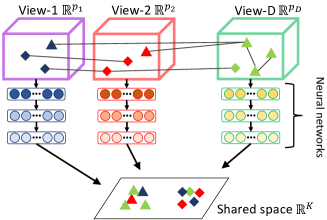
Figure 1: Data vectors $\{\boldsymbol{x}_{i}\}$ in each view are transformed to feature vectors $\{\boldsymbol{y}_{i}\}$ by neural networks $\{f^{(d)}_{\boldsymbol{\psi}}\}$.

These transformations $\{f^{(d)}_{\boldsymbol{\psi}}\}$ can be trained by maximizing the likelihood for the probabilistic model (1) as shown in Section 3.5. PMvGE computes feature vectors $\{\boldsymbol{y}_{i}\}_{i=1}^{n}$ through maximum likelihood estimation of transformations $\{f^{(d)}_{\boldsymbol{\psi}}\}$.

PMvGE associates nodes $v_{i}$ and $v_{j}$ with the probability specified by the similarity between their feature vectors $\boldsymbol{y}_{i}:=f^{(d_{i})}_{\boldsymbol{\psi}}(\boldsymbol{x}_{i}),\boldsymbol{y}_{j}:=f^{(d_{j})}_{\boldsymbol{\psi}}(\boldsymbol{x}_{j})\in\mathbb{R}^{K}$ in the shared space. Nodes with similar feature vectors will share many links.

We consider the following neural network model for the transformation function, while any functional form can be accepted for PMvGE. Only the inner product of feature vectors is considered for measuring the similarity in PMvGE. We prove in Theorem 5.1 that the inner product with neural networks approximates a wide class of similarity measures.

Neural Network (NN) with 3-layers is defined as

$$f^{(d)}_{\boldsymbol{\psi}}(\boldsymbol{x})=\boldsymbol{\sigma}(\boldsymbol{\psi}^{(d)\top}_{3}\boldsymbol{\sigma}(\boldsymbol{\psi}^{(d)\top}_{2}\boldsymbol{\sigma}(\boldsymbol{\psi}^{(d)\top}_{1}\boldsymbol{x})))),$$ (4)

where $\boldsymbol{x}\in\mathbb{R}^{p_{d}}$ is data vector, $\boldsymbol{\psi}^{(d)}_{1}\in\mathbb{R}^{p_{d}\times K^{(d)}_{1}},\boldsymbol{\psi}^{(d)}_{2}\in\mathbb{R}^{K^{(d)}_{1}\times K^{(d)}_{2}},\boldsymbol{\psi}^{(d)}_{3}\in\mathbb{R}^{K^{(d)}_{2}\times K}$ are parameter matrices. The neural network size is specified by $p_{d},K_{1}^{(d)},K_{2}^{(d)},K\in\mathbb{N}$ $(d=1,2,\ldots,D)$. Each element of $\boldsymbol{\sigma}(\boldsymbol{x})$ is user-specified activation function $\sigma(\cdot)$. Although we basically consider a multi-layer perceptron (MLP) as $f^{(d)}_{\boldsymbol{\psi}}$, it can be replaced with any deterministic NN with input and output layers, such as recurrent NN and Deep NN (DNN).

NN model reduces to linear model

$$f^{(d)}_{\boldsymbol{\psi}}(\boldsymbol{x}):=\boldsymbol{\psi}^{(d)\top}\boldsymbol{x}$$ (5)

$(d=1,2,\ldots,D)$ by applying $\sigma(x)=x$, where $\boldsymbol{\psi}^{(d)}\in\mathbb{R}^{p_{d}\times K}$ is parameter matrix.

3.4 Link weights across some view pairs may be missing

Link weights across all the view pairs may not be available in practice. So we consider the set of unordered view pairs

$$\mathcal{D} :=\{(d,e)\text{ : Link weights are}$$

$$\hskip 70.0001pt\text{observed between views $d,e$}\},$$

and we formally set $w_{ij}=0$ for the missing $(d_{i},d_{j})\notin\mathcal{D}$. For example, $\mathcal{D}=\{(1,2)\}$ for $D=2$ indicates that link weights across view-1 and view-2 are observed while link weights within view-1 or view-2 are missing. We should notice the distinction between setting $w_{ij}=0$ with missing and observing $w_{ij}=0$ without missing, because these two cases give different likelihood functions.

3.5 Maximum Likelihood Estimator

Since PMvGE is specified by (1) and (3), the log-likelihood function is given by

$${\ell}_{n}(\boldsymbol{\alpha}, \boldsymbol{\psi})$$

$$:= \sum_{(i,j)\in\mathcal{I}_{n}}[w_{ij}\log\mu_{ij}(\boldsymbol{\alpha},\boldsymbol{\psi})-\mu_{ij}(\boldsymbol{\alpha},\boldsymbol{\psi})],$$ (6)

whose sum is over the set of index pairs $\mathcal{I}_{n}:=\{(i,j)\mid 1\leq i<j\leq n,(d_{i},d_{j})\in\mathcal{D}\}$. The Maximum Likelihood Estimator (MLE) of the parameter $(\boldsymbol{\alpha},\boldsymbol{\psi})$ is defined as the maximizer of (6). We estimate $(\boldsymbol{\alpha},\boldsymbol{\psi})$ by maximizing ${\ell}_{n}(\boldsymbol{\alpha},\boldsymbol{\psi})$ with constraints $\boldsymbol{\alpha}=\boldsymbol{\alpha}^{\top}$ and $\alpha^{(d,e)}=0$ for $(d,e)\notin\mathcal{D}$.

3.6 PMvGE approximately generalizes various methods for multi-view learning

SBM (2) is 1-view PMvGE with 1-hot cluster membership vector $\boldsymbol{x}_{i}\in\{0,1\}^{C}$. Consider the linear model (5) with $\boldsymbol{\psi}^{(1)\top}=(\boldsymbol{\psi}^{1},\ldots,\boldsymbol{\psi}^{C})\in\mathbb{R}^{K\times C}$, where $\boldsymbol{\psi}^{c}\in\mathbb{R}^{K}$ is a feature vector for class $c=1,\ldots,C$. Then $\mu_{ij}=\alpha^{(1,1)}\exp(\langle\boldsymbol{\psi}^{c_{i}},\boldsymbol{\psi}^{c_{j}}\rangle)$ will specify $\beta^{(c_{i},c_{j})}$ for sufficiently large $K$, and $\{\boldsymbol{\psi}^{c_{i}}\}$ represent low-dimensional structure of SBM for smaller $K$. SBM is also interpreted as PMvGE with $D=C$ views by letting $d_{i}=c_{i}$ and $f^{(d_{i})}_{\boldsymbol{\psi}}(\boldsymbol{x})\equiv 0$. Then $\mu_{ij}=\alpha^{(c_{i},c_{j})}$ is equivalent to SBM.

More generally, CDMCA (Shimodaira,, 2016) is approximated by $D$-view PMvGE with the linear transformations (5). The first half of the objective function (6) becomes

$$\frac{1}{2}\sum_{i=1}^{n}\sum_{j=1}^{n}w_{ij}\langle\boldsymbol{\psi}^{(d_{i})\top}\boldsymbol{x}_{i},\boldsymbol{\psi}^{(d_{j})\top}\boldsymbol{x}_{j}\rangle$$ (7)

by specifying $\alpha^{(d,e)}\equiv 1$. CDMCA computes the transformation matrices $\{\boldsymbol{\psi}^{(d)}\}$ by maximizing this objective function under a quadratic constraint such as

$$\sum_{i=1}^{n}\sum_{j=1}^{n}w_{ij}\boldsymbol{\psi}^{(d_{i})\top}\boldsymbol{x}_{i}\boldsymbol{x}_{i}^{\top}\boldsymbol{\psi}^{(d_{i})}=\boldsymbol{I}.$$ (8)

The above observation intuitively explains why PMvGE approximates CDMCA; this is more formally discussed in Supplement C. The quadratic constraint is required for preventing the maximizer of (7) from being diverged in CDMCA. However, our likelihood approach does not require it, because the last half of (6) serves as a regularization term.

3.7 PMvGE represents neural network classifiers of multiple classes

For illustrating the generality of PMvGE, here we consider the multi-class classification problem. We show that PMvGE includes Feed-Forward Neural Network (FFNN) classifier as a special case.

Let $(\boldsymbol{x}_{i},c_{i})\in\mathbb{R}^{p}\times\{1,\ldots,C\}$, $i=1,\ldots,n$ be the training data for the classification problem of $C$ classes. FFNN classifier with softmax function (Bishop,, 2006) is defined as

$$h_{j}(\boldsymbol{x}_{i}):=\frac{\exp(f_{\boldsymbol{\psi},j}(\boldsymbol{x}_{i}))}{\sum_{j=1}^{C}\exp(f_{\boldsymbol{\psi},j}(\boldsymbol{x}_{i}))},\quad j=1,\ldots,C,$$

where $f_{\boldsymbol{\psi}}(\boldsymbol{x}):=(f_{\boldsymbol{\psi},1}(\boldsymbol{x}),\ldots,f_{\boldsymbol{\psi},C}(\boldsymbol{x}))\in\mathbb{R}^{C}_{\geq 0}$ is a multi-valued neural network, and $\boldsymbol{x}_{i}$ is classified into the class $\displaystyle\mathop{\arg\max}_{j\in\{1,2,\ldots,C\}}h_{j}(\boldsymbol{x}_{i})$. This classifier is equivalent to

$$\mathop{\arg\max}_{j\in\{1,2,\ldots,C\}}\exp\left(\langle f_{\boldsymbol{\psi}}(\boldsymbol{x}_{i}),\boldsymbol{e}_{j}\rangle\right),$$ (9)

where $\boldsymbol{e}_{j}\in\{0,1\}^{C}$ is the 1-hot vector with 1 at $j$-th entry and 0 otherwise.

The classifier (9) can be interpreted as PMvGE with $D=2,\mathcal{D}=\{(1,2)\}$ as follows. For view-1, $f^{(1)}_{\boldsymbol{\psi}}(\boldsymbol{x}):=f_{\boldsymbol{\psi}}(\boldsymbol{x})$ and inputs are $\boldsymbol{x}_{1},\ldots,\boldsymbol{x}_{n}$. For view-2, $f^{(2)}_{\boldsymbol{\psi}}(\boldsymbol{x}^{\prime}):=\boldsymbol{x}^{\prime}$ and inputs are $\boldsymbol{e}_{1},\ldots,\boldsymbol{e}_{C}$. We set $w_{ij}=1$ between $\boldsymbol{x}_{i}$ and $\boldsymbol{e}_{c_{i}}$, and $w_{ij}=0$ otherwise.

4 Optimization

In this section, we present an efficient way of optimizing the parameters for maximizing the objective function ${\ell}_{n}(\boldsymbol{\alpha},\boldsymbol{\psi})$ defined in eq. (6). We alternatively optimize the two parameters $\boldsymbol{\alpha}$ and $\boldsymbol{\psi}$. Efficient update of $\boldsymbol{\psi}$ with minibatch SGD is considered in Section 4.1, and update of $\boldsymbol{\alpha}$ by solving an estimating equation is considered in Section 4.2. We iterate these two steps for maximizing ${\ell}_{n}(\boldsymbol{\alpha},\boldsymbol{\psi})$.

4.1 Update of $\boldsymbol{\psi}$

We update $\boldsymbol{\psi}$ using the gradient of ${\ell}_{n}(\bar{\boldsymbol{\alpha}},\boldsymbol{\psi})$ by fixing current parameter value $\bar{\boldsymbol{\alpha}}$. Since $\boldsymbol{W}=(w_{ij})$ may be sparse in practice, the computational cost of minibatch SGD (Goodfellow et al.,, 2016) for the first half of ${\ell}_{n}(\bar{\boldsymbol{\alpha}},\boldsymbol{\psi})$ is expected to be reduced by considering the sum over the set $\mathcal{W}_{n}:=\{(i,j)\in\mathcal{I}_{n}\mid w_{ij}>0\}$. On the other hand, there should be $|\mathcal{I}_{n}|=O(n^{2})$ positive terms in the last half of ${\ell}_{n}(\bar{\boldsymbol{\alpha}},\boldsymbol{\psi})$, so we consider the sum over node pairs uniformly-resampled from $\mathcal{I}_{n}$.

We make two sets $\mathcal{I}^{\prime}_{n},\mathcal{W}^{\prime}_{n}$ by picking $(i,j)$ from $\mathcal{I}_{n}$ and $\mathcal{W}_{n}$, respectively, so that

$$|\mathcal{I}_{n}^{\prime}|+|\mathcal{W}^{\prime}_{n}|=m,\>|\mathcal{I}_{n}^{\prime}|/|\mathcal{W}^{\prime}_{n}|=r.$$

User-specified constants $m\in\mathbb{N}$ and $r>0$ are usually called as “minibatch size” and “negative sampling rate”. We sequentially update minibatch $\mathcal{I}^{\prime}_{n},\mathcal{W}^{\prime}_{n}$ for computing the gradient of

(10)

with respect to $\boldsymbol{\psi}$. By utilizing the gradient, the parameter $\boldsymbol{\psi}$ can be sequentially updated by SGD, where $\tau>0$ is a tuning parameter. Eq. (10) approximates ${\ell}_{n}(\bar{\boldsymbol{\alpha}},\boldsymbol{\psi})$ if $(i,j)$ are uniformly-resampled and $\tau=|\mathcal{I}_{n}|/(r\,|\mathcal{W}_{n}|)$, however, smaller $\tau$ such as $\tau=1$ may make this algorithm stable in some cases.

4.2 Update of $\boldsymbol{\alpha}$

Let $\bar{\boldsymbol{\psi}}$ represent current parameter value of $\boldsymbol{\psi}$. By solving the estimating equation $\frac{\partial{\ell}_{n}(\boldsymbol{\alpha},\bar{\boldsymbol{\psi}})}{\partial\alpha^{(d,e)}}=0$ with respect to $\alpha^{(d,e)}$ under constraints $\boldsymbol{\alpha}=\boldsymbol{\alpha}^{\top}$ and $\alpha^{(d,e)}=0$, $(d,e)\notin\mathcal{D}$, we explicitly obtain a local maximizer of ${\ell}_{n}(\boldsymbol{\alpha},\bar{\boldsymbol{\psi}})$. However, the local maximizer requires roughly $O(n^{2})$ operations for computation. To reduce the high computational cost, we efficiently update $\boldsymbol{\alpha}$ by (11), which is a minibatch-based approximation of the local maximizer.

(11)

where $\bar{g}_{ij}:=\langle f^{(d)}_{\bar{\boldsymbol{\psi}}}(\boldsymbol{x}_{i}),f^{(e)}_{\bar{\boldsymbol{\psi}}}(\boldsymbol{x}_{j})\rangle$, $\mathcal{I}_{n}^{{}^{\prime}(d,e)}:=\{(i,j)\in\mathcal{I}^{\prime}_{n}\mid(d_{i},d_{j})=(d,e)\}$, and $\mathcal{I}^{\prime}_{n}$ is the minibatch defined in Section 4.1. Note that $(d,e)$ is unordered view pair.

4.3 Computational cost

PMvGE requires $O(m)$ operations for each minibatch iteration. It is efficiently computed even if the number of data vectors $n$ is very large.

5 PMvGE learns arbitrary similarity measure

Two theoretical results are shown here for indicating that PMvGE with sufficiently large neural networks learns arbitrary similarity measure using sufficiently many data vectors. In Section 5.1, we prove that arbitrary similarity measure can be approximated by the inner product in the shared space with sufficiently large neural networks. In Section 5.2, we prove that MLE of PMvGE converges to the true parameter value, i.e., the consistency of MLE, in some sense as the number of data vectors increases.

5.1 Inner product of NNs approximates a wide class of similarity measures across views

Feedforward neural networks with ReLU or sigmoid function are proved to be able to approximate arbitrary continuous functions under some assumptions (Cybenko,, 1989; Funahashi,, 1989; Yarotsky,, 2016; Telgarsky,, 2017). However, these results cannot be directly applied to PMvGE, because our model is based on the inner product of two neural networks $\langle f_{\boldsymbol{\psi}}^{(d_{i})}(\boldsymbol{x}_{i}),f_{\boldsymbol{\psi}}^{(d_{j})}(\boldsymbol{x}_{j})\rangle$. In Theorem 5.1, we show that the inner product can approximate $g_{*}\left(f_{*}^{(d_{i})}(\boldsymbol{x}_{i}),f_{*}^{(d_{j})}(\boldsymbol{x}_{j})\right)$, that is, arbitrary similarity measure $g_{*}(\cdot,\cdot)$ in $K_{*}$ dimensional shared space, where $f_{*}^{(d_{i})}$, $f_{*}^{(d_{j})}$ are arbitrary two continuous functions. For showing $g_{*}(f_{*}^{(d)}(\boldsymbol{x}),f_{*}^{(e)}(\boldsymbol{x}^{\prime}))\approx\langle f_{\boldsymbol{\psi}}^{(d)}(\boldsymbol{x}),f_{\boldsymbol{\psi}}^{(e)}(\boldsymbol{x}^{\prime})\rangle$, the idea is first consider a feature map $\boldsymbol{\Phi}_{K}:\mathbb{R}^{K^{*}}\to\mathbb{R}^{K}$ for approximating $g_{*}(\boldsymbol{y}_{*},\boldsymbol{y}^{\prime}_{*})\approx\langle\boldsymbol{\Phi}_{K}(\boldsymbol{y}_{*}),\boldsymbol{\Phi}_{K}(\boldsymbol{y}_{*}^{\prime})\rangle$ with sufficiently large $K$, and then consider neural networks $f_{\boldsymbol{\psi}}^{(d)}:\mathbb{R}^{p_{d}}\to\mathbb{R}^{K}$ with sufficiently many hidden units for approximating $\boldsymbol{\Phi}_{K}(f_{*}^{(d)}(\boldsymbol{x}))\approx f_{\boldsymbol{\psi}}^{(d)}(\boldsymbol{x})$.

Theorem 5.1

Let $f^{(d)}_{*}:[-M,M]^{p_{d}}\to[-M^{\prime},M^{\prime}]^{K_{*}}$, $d=1,2,\ldots,D$, be continuous functions and $g_{*}:[-M^{\prime},M^{\prime}]^{K_{*}}\times[-M^{\prime},M^{\prime}]^{K_{*}}\to\mathbb{R}$ be a symmetric, continuous, and positive-definite kernel function for some $K^{*},M,M^{\prime}>0$. $\sigma(\cdot)$ is ReLU or activation function which is non-constant, continuous, bounded, and monotonically-increasing. Then, for arbitrary $\varepsilon>0$, by specifying sufficiently large $K\in\mathbb{N},T=T(K)\in\mathbb{N}$, there exist $\boldsymbol{A}^{d}\in\mathbb{R}^{K\times T},\boldsymbol{B}^{d}\in\mathbb{R}^{T\times p_{d}},\boldsymbol{c}\in\mathbb{R}^{T}$, $d\in\{1,2,\ldots,D\}$, such that

for all $(\boldsymbol{x},\boldsymbol{x}^{\prime})\in[-M,M]^{p_{d}+p_{e}}$, $d,e\in\{1,2,\ldots,D\}$, where $f_{\boldsymbol{\psi}}^{(d)}(\boldsymbol{x}^{d})=\boldsymbol{A}^{d}\boldsymbol{\sigma}(\boldsymbol{B}^{d}\boldsymbol{x}^{d}+\boldsymbol{c}^{d})$, $d=1,2,\ldots,D$, are two-layer neural networks with $T$ hidden units and $\boldsymbol{\sigma}(\boldsymbol{x})$ is element-wise $\sigma(\cdot)$ function.

Proof of the theorem is given in Supplement A.

If $D=1$, Theorem 5.1 corresponds to Mercer’s theorem (Mercer,, 1909; Courant and Hilbert,, 1989) of Kernel methods, which states that arbitrary positive definite kernel $g_{*}(\cdot,\cdot)$ can be expressed as the inner product of high-dimensional feature maps. While Mercer’s theorem indicates only the existence of such feature maps, Theorem 5.1 also states that the feature maps can be approximated by neural networks.

Illustrative example As an example of positive definite similarity, we consider the cosine similarity

$$g_{*}(f_{*}(\boldsymbol{x}),f_{*}(\boldsymbol{x}^{\prime})):=\frac{\langle f_{*}(\boldsymbol{x}),f_{*}(\boldsymbol{x}^{\prime})\rangle}{\|f_{*}(\boldsymbol{x})\|_{2}\|f_{*}(\boldsymbol{x}^{\prime})\|_{2}}$$

with $f_{*}(\boldsymbol{x})=(x_{1},\cos x_{2},\exp(-x_{3}),\sin(x_{4}-x_{5})),p=5$. For 2-dim visualization in Fig. 2 with $(s,t)\in\mathbb{R}^{2}$, let us define $G_{*}(s,t):=g_{*}(f_{*}(s\boldsymbol{e}_{1}),f_{*}(t\boldsymbol{e}_{2})),\boldsymbol{e}_{1}:=(1,1,1,0,0),\boldsymbol{e}_{2}:=(0,0,1,1,1)$ and its approximation by the inner product of neural networks $\hat{G}_{K}(s,t):=\langle f_{\boldsymbol{\psi}}(s\boldsymbol{e}_{1}),f_{\boldsymbol{\psi}}(t\boldsymbol{e}_{2})\rangle$ with $T=10^{3}$ hidden units. If $K$ and $T$ are sufficiently large, $\hat{G}_{K}(s,t)$ approximates $G_{*}(s,t)$ very well as suggested by Theorem 5.1.

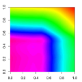
(a) $\hat{G}_{2}(s,t)$

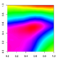
(b) $\hat{G}_{50}(s,t)$

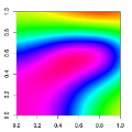
(c) $G_{*}(s,t)$

Figure 2: A two-dim visualization $G_{*}(s,t)$ of similarity measure $g_{*}(\boldsymbol{y}_{*},\boldsymbol{y}_{*}^{\prime})=\frac{\langle\boldsymbol{y},\boldsymbol{y}^{\prime}\rangle}{\|\boldsymbol{y}\|_{2}\|\boldsymbol{y}^{\prime}\|_{2}}$ with $K_{*}=2$ is well approximated by the visualization $\hat{G}_{K}(s,t)$ of the inner product $\langle\boldsymbol{y},\boldsymbol{y}^{\prime}\rangle$ for $K=100$, while the approximation is poor for $K=2$. A neural network $f_{\boldsymbol{\psi}}$ with $T=10^{3}$ ReLU units and $K=2$ or $K=50$ linear output units are trained with $n=10^{3}$ data vectors and link weights across views.

5.2 MLE converges to the true parameter value

We have shown the universal approximation theorem of similarity measure in Theorem 5.1. However, it only states that the good approximation is achieved if we properly tune the parameters of neural networks. Here we argue that MLE of Section 3.5 will actually achieve the good approximation if we have sufficiently many data vectors. The technical details of the argument are given in Supplement B.

Let $\boldsymbol{\theta}\in\boldsymbol{\Theta}$ denote the vector of free parameters in $\boldsymbol{\alpha},\boldsymbol{\psi}$, and $\ell_{n}(\boldsymbol{\theta})$ be the log-likelihood function (6). We assume that the optimization algorithm in Section 4 successfully computes MLE $\hat{\boldsymbol{\theta}}_{n}$ that maximizes $\ell_{n}(\boldsymbol{\theta})$. Here we ignore the difficulty of global optimization, while we may only get a local maximum in practice. We also assume that PMvGE is correctly specified; there exists a parameter value $\boldsymbol{\theta}_{*}$ so that the parametric model represents the true probability distribution.

Then, we would like to claim that $\hat{\boldsymbol{\theta}}_{n}$ converges to the true parameter value $\boldsymbol{\theta}_{*}$ in the limit of $n\to\infty$, the property called the consistency of MLE. However, we have to pay careful attention to the fact that PMvGE is not a standard setting in the sense that (i) there are correlated $O(n^{2})$ samples instead of $n$ i.i.d. observations, and (ii) the model is not identifiable with infinitely many equivalent parameter values; for example there are rotational degrees of freedom in the shared space so that $\langle\boldsymbol{y},\boldsymbol{y}^{\prime}\rangle=\langle\boldsymbol{O}\boldsymbol{y},\boldsymbol{O}\boldsymbol{y}^{\prime}\rangle$ with any orthogonal matrix $\boldsymbol{O}$ in $\mathbb{R}^{K}$. We then consider the set of equivalent parameters $\hat{\boldsymbol{\Theta}}_{n}:=\{\boldsymbol{\theta}\in\boldsymbol{\Theta}\mid\ell_{n}(\boldsymbol{\theta})=\ell_{n}(\hat{\boldsymbol{\theta}}_{n})\}$. Theorem B.2 states that, as $n\to\infty$, $\hat{\boldsymbol{\Theta}}_{n}$ converges to $\boldsymbol{\Theta}_{*}$, the set of $\boldsymbol{\theta}$ values equivalent to $\boldsymbol{\theta}_{*}$.

6 Real data analysis

6.1 Experiments on Citation dataset (1-view)

Dataset: We use Cora dataset (Sen et al.,, 2008) of citation network with 2,708 nodes and 5,278 ordered edges. Each node $v_{i}$ represents a document, which has $1,433$-dimensional (bag-of-words) data vector $\boldsymbol{x}_{i}\in\{0,1\}^{1433}$ and a class label of 7 classes. Each directed edge represents citation from a document $v_{i}$ to another document $v_{j}$. We set the link weight as $w_{ij}=w_{ji}=1$ by ignoring the direction, and $w_{ij}=0$ otherwise. There is no cross or self-citation. We divide the dataset into training set consisting of $2,166$ nodes ($80\%$) with their edges, and test set consisting of remaining $542$ nodes ($20\%$) with their edges. We utilize $20\%$ of the training set for validation. Hyper-parameters are tuned by utilizing the validation set.

We compare PMvGE with several feature learning methods: Stochastic Block Model (Holland et al.,, 1983, SBM), ISOMAP (Tenenbaum et al.,, 2000), Locally Linear Embedding (Roweis and Saul,, 2000, LLE), Spectral Graph Embedding (Belkin and Niyogi,, 2001, SGE), Multi Dimensional Scaling (Kruskal,, 1964, MDS), DeepWalk (Perozzi et al.,, 2014), and GraphSAGE (Hamilton et al.,, 2017).

NN for PMvGE: 2-layer fully-connected network, which consists of 3,000 tanh hidden units and 1,000 tanh output units, is used. The network is trained by Adam (Kingma and Ba,, 2015) with batch normalization. The learning rate is starting from $0.0001$ and attenuated by $1/10$ for every 100 iterations. Negative sampling rate $r$ and minibatch size $m$ are set as $1$ and $512$, respectively, and the number of iterations is $200$.

Parameter tuning: For each method, parameters are tuned on validation sets. Especially, the dimension of feature vectors is selected from $\{50,100,150,200\}$.

Label classification (Task 1): We classify the documents into 7 classes using logistic regression with the feature vector as input and the class label as output. We utilize LibLinear (Fan et al.,, 2008) for the implementation.

Clustering (Task 2): The $k$-means clustering of the feature vectors is performed for unsupervised learning of document clusters. The number of clusters is set as $7$.

Results: The quality of classification is evaluated by classification accuracy in Task 1, and Normalized Mutual Information (NMI) in Task 2. Sample averages and standard deviations over 10 experiments are shown in Table 2. In experiment (A), we apply methods to both training set and test set, and evaluate them by test set. In (B), we apply methods to only the training set, and evaluate them by test set. SGE, MDS, and DeepWalk are not inductive, and they cannot be applied to unseen data vectors in (B). PMvGE outperforms the other methods in both experiments.

6.2 Experiments on AwA dataset (2-view)

Dataset: We use Animal with Attributes (AwA) dataset (Lampert et al.,, 2009) with 30,475 images for view-1 and 85 attributes for view-2. We prepared $4,096$ dimensional DeCAF data vector (Donahue et al.,, 2014) for each image, and $300$ dimensional GloVe (Pennington et al.,, 2014) data vector for each attribute. Each image is associated with some attributes. We set $w_{ij}=1$ for the associated pairs between the two views, and $w_{ij}=0$ otherwise. In addition to the attributes, each image has a class label of 50 classes. We resampled 50 images from each of 50 classes; in total, 2500 images. In each experiment, we split the 2500 images into 1500 training images and 100 test images. A validation set of 300 images is sampled from the training images.

We compare PMvGE with CCA, DCCA (Andrew et al.,, 2013), SGE, DeepWalk, and GraphSAGE.

NN for PMvGE: Each view uses a 2-layer fully-connected network, which consists of 2000 tanh hidden units and 100 tanh output units. The dimension of the feature vector is $K=100$. Adam is used for optimization with Batch normalization and Dropout ($p=0.5$). Minibatch size, learning rate, and momentum are tuned on the validation set. We monitor the score on the validation set for early stopping.

Parameter tuning: For each method, parameters are tuned on validation sets. Especially, the dimension of feature vectors is selected from $\{10,50,100,150\}$.

Link prediction (Task 3): For each query image, we rank attributes according to the cosine similarity of feature vectors across views. An attribute is regarded as correct if it is associated with the query image.

Results: The quality of the ranked list of attributes is measured by Average Precision (AP) score in Task 3. Sample averages and standard deviations over 10 experiments are shown in Table 2. In experiment (A), we apply methods to both training set and test set, and evaluate them by test set. The whole training set is used for validation. In experiment (B), we apply methods to only the training set, and evaluate them by test set. 20$\%$ of training set is used for validation. PMvGE outperforms the other methods including DCCA. While DeepWalk shows good performance in experiment (A), DeepWalk and SGE cannot be applied to unseen data vectors in (B). Unlike SGE and DeepWalk which only consider the associations, 1-view feature learning methods such as GraphSAGE cannot be applied to this AwA dataset since the dimension of data vectors is different depending on the view. So we do not perform 1-view methods in Task 3.

Table 2: Task 1 and Task 2 for the experiment on Citation dataset ($D=1$), and Task 3 for the experiment on AwA dataset ($D=2$). The larger values are better.

		(A)	(B)
Task 1 ($D=1$)	ISOMAP	$54.5\pm 1.78$	$54.8\pm 2.43$
	LLE	$30.2\pm 1.91$	$31.9\pm 2.62$
	SGE	$47.6\pm 1.64$	-
	MDS	$29.8\pm 2.25$	-
	DeepWalk	$54.2\pm 2.04$	-
	GraphSAGE	$60.8\pm 1.73$	$57.1\pm 1.61$
	PMvGE	$\mathbf{74.8\pm 2.55}$	$\mathbf{71.1\pm 2.10}$
Task 2 ($D=1$)	SBM	$4.37\pm 1.44$	$2.81\pm 0.10$
	ISOMAP	$13.0\pm 0.36$	$14.3\pm 1.98$
	LLE	$7.40\pm 3.40$	$9.47\pm 3.00$
	SGE	$1.41\pm 0.34$	-
	MDS	$2.81\pm 0.10$	-
	DeepWalk	$16.7\pm 1.05$	-
	GraphSAGE	$19.6\pm 0.93$	$12.4\pm 3.00$
	PMvGE	$\mathbf{35.9\pm 0.88}$	$\mathbf{30.5\pm 3.90}$
Task 3 ($D=2$)	CCA	$45.5\pm 0.20$	$42.4\pm 0.30$
	DCCA	$41.4\pm 0.30$	$41.2\pm 0.35$
	SGE	$43.5\pm 0.39$	-
	DeepWalk	$71.3\pm 0.57$	-
	PMvGE	$\mathbf{71.5\pm 0.48}$	$\mathbf{70.5\pm 0.53}$

Locality of each-view is preserved through neural networks: To see whether the locality of input is preserved through neural networks in PMvGE, we computed the Spearman’s rank correlation coefficient between $\langle\boldsymbol{x},\boldsymbol{x}^{\prime}\rangle$ and $\langle f_{\boldsymbol{\psi}}^{(d)}(\boldsymbol{x}),f_{\boldsymbol{\psi}}^{(d)}(\boldsymbol{x}^{\prime})\rangle$ for view-$d$ data vectors $\boldsymbol{x},\boldsymbol{x}^{\prime}$ in AwA dataset ($d=1,2$). For DeCAF (view-1) and GloVe (view-2) inputs, the values are $0.722\pm 0.058$ and $0.811\pm 0.082$, respectively. This result indicates that the feature vectors of PMvGE preserves the similarities of the data vectors fairly well.

7 Conclusion

We presented a simple probabilistic framework for multi-view learning with many-to-many associations. We name the framework as Probabilistic Multi-view Graph Embedding (PMvGE). Various existing methods are approximately included in PMvGE. We gave theoretical justification and practical estimation algorithm to PMvGE. Experiments on real-world datasets showed that PMvGE outperforms existing methods.

Supplementary Material: A probabilistic framework for multi-view feature learning with many-to-many associations via neural networks

Appendix A Proof of Theorem 5.1

Since $g_{*}:[-M^{\prime},M^{\prime}]^{2K_{*}}\to\mathbb{R}$ is a positive definite kernel on a compact set, it follows from Mercer’s theorem that there exist positive eigenvalues $\{\lambda_{k}\}_{k=1}^{\infty}$ and continuous eigenfunctions $\{\phi_{k}\}_{k=1}^{\infty}$ such that

$$g_{*}(\boldsymbol{y}_{*},\boldsymbol{y}_{*}^{\prime})=\sum_{k=1}^{\infty}\lambda_{k}\phi_{k}(\boldsymbol{y}_{*})\phi_{k}(\boldsymbol{y}_{*}^{\prime}),\quad\boldsymbol{y}_{*},\boldsymbol{y}_{*}^{\prime}\in[-M^{\prime},M^{\prime}]^{K_{*}},$$

where the convergence is absolute and uniform (Minh et al.,, 2006). The uniform convergence implies that for any $\varepsilon_{1}>0$ there exists $K_{0}\in\mathbb{N}$ such that

$$\sup_{(\boldsymbol{y}_{*},\boldsymbol{y}_{*}^{\prime})\in[-M^{\prime},M^{\prime}]^{2K_{*}}}\bigg{|}g_{*}(\boldsymbol{y}_{*},\boldsymbol{y}_{*}^{\prime})-\sum_{k=1}^{K}\lambda_{k}\phi_{k}(\boldsymbol{y}_{*})\phi_{k}(\boldsymbol{y}_{*}^{\prime})\bigg{|}<\varepsilon_{1},\quad K\geq K_{0}.$$

This means $g_{*}(\boldsymbol{y}_{*},\boldsymbol{y}^{\prime}_{*})\approx\langle\boldsymbol{\Phi}_{K}(\boldsymbol{y}_{*}),\boldsymbol{\Phi}_{K}(\boldsymbol{y}_{*}^{\prime})\rangle$ for a feature map $\boldsymbol{\Phi}_{K}(\boldsymbol{y}_{*})=(\sqrt{\lambda_{k}}\phi_{k}(\boldsymbol{y}_{*}))_{k=1}^{K}$.

We fix $K$ and consider approximation of $h_{k}^{(d)}(\boldsymbol{x}):=\sqrt{\lambda_{k}}\phi_{k}(f_{*}^{(d)}(\boldsymbol{x}))$ below. Since $h_{k}^{(d)}$ are continuous functions on a compact set, there exists $C=C(K)>0$ such that

$$\sup_{\boldsymbol{x}\in[-M,M]^{p_{d}}}|h_{k}^{(d)}(\boldsymbol{x})|<C,\quad k=1,\ldots,K,\,d=1,\ldots,D.$$

Let us write the neural networks as $f_{\boldsymbol{\psi}}^{(d)}=(f_{1}^{(d)},\ldots,f_{K}^{(d)})$, where $f_{k}^{(d)}:\mathbb{R}^{p_{d}}\to\mathbb{R}$, $d=1,\ldots,D$, $k=1,\ldots,K$, are two-layer neural networks with $T$ hidden units. Since $h_{k}^{(d)}$ are continuous functions, it follows from the universal approximation theorem (Cybenko,, 1989; Telgarsky,, 2017) that for any $\varepsilon_{2}>0$, there exists $T_{0}(K)\in\mathbb{N}$ such that

$$\sup_{\boldsymbol{x}\in[-M,M]^{p_{d}}}|h_{k}^{(d)}(\boldsymbol{x})-f_{k}^{(d)}(\boldsymbol{x})|<\varepsilon_{2},\quad k=1,\ldots,K,\,d=1,\ldots,D$$

for $T\geq T_{0}(K)$. Therefore, for all $d,e\in\{1,2,\ldots,D\}$, we have

$$\sup_{(\boldsymbol{x},\boldsymbol{x}^{\prime})\in[-M,M]^{p_{d}+p_{e}}} \biggl{|}g_{*}\left(f^{(d)}_{*}(\boldsymbol{x}),f^{(e)}_{*}(\boldsymbol{x}^{\prime})\right)-\sum_{k=1}^{K}f_{k}^{(d)}(\boldsymbol{x})f_{k}^{(e)}(\boldsymbol{x}^{\prime})\biggr{|}$$

$$\leq\sup_{(\boldsymbol{x},\boldsymbol{x}^{\prime})\in[-M,M]^{p_{d}+p_{e}}}\biggl{|}g_{*}\left(f^{(d)}_{*}(\boldsymbol{x}),f^{(e)}_{*}(\boldsymbol{x}^{\prime})\right)-\sum_{k=1}^{K}h_{k}^{(d)}(\boldsymbol{x})h_{k}^{(e)}(\boldsymbol{x}^{\prime})\biggr{|}$$

$$\hskip 20.00003pt+\sup_{(\boldsymbol{x},\boldsymbol{x}^{\prime})\in[-M,M]^{p_{d}+p_{e}}}\biggl{|}\sum_{k=1}^{K}h_{k}^{(d)}(\boldsymbol{x})\left(h_{k}^{(e)}(\boldsymbol{x}^{\prime})-f_{k}^{(e)}(\boldsymbol{x}^{\prime})\right)\biggr{|}$$

$$\hskip 20.00003pt+\sup_{(\boldsymbol{x},\boldsymbol{x}^{\prime})\in[-M,M]^{p_{d}+p_{e}}}\biggl{|}\sum_{k=1}^{K}\left(h_{k}^{(d)}(\boldsymbol{x})-f_{k}^{(d)}(\boldsymbol{x})\right)f_{k}^{(e)}(\boldsymbol{x}^{\prime})\biggr{|}$$

$$\leq\sup_{\boldsymbol{y}_{*},\boldsymbol{y}_{*}^{\prime}\in[-M^{\prime},M^{\prime}]^{K_{*}}}\biggl{|}g_{*}\left(\boldsymbol{y}_{*},\boldsymbol{y}_{*}^{\prime}\right)-\sum_{k=1}^{K}\lambda_{k}\phi_{k}(\boldsymbol{y}_{*})\phi_{k}(\boldsymbol{y}_{*}^{\prime})\biggr{|}$$

$$\hskip 20.00003pt+\sum_{k=1}^{K}\sup_{\boldsymbol{x}\in[-M,M]^{p_{d}}}|h_{k}^{(d)}(\boldsymbol{x})|\sup_{\boldsymbol{x}^{\prime}\in[-M,M]^{p_{e}}}\left|h_{k}^{(e)}(\boldsymbol{x}^{\prime})-f_{k}^{(e)}(\boldsymbol{x}^{\prime})\right|$$

$$\hskip 20.00003pt+\sum_{k=1}^{K}\sup_{\boldsymbol{x}\in[-M,M]^{p_{d}}}\left|h_{k}^{(d)}(\boldsymbol{x})-f_{k}^{(d)}(\boldsymbol{x})\right|\sup_{\boldsymbol{x}^{\prime}\in[-M,M]^{p_{e}}}|f_{k}^{(e)}(\boldsymbol{x}^{\prime})|$$

$$<\varepsilon_{1}+KC\varepsilon_{2}+K\varepsilon_{2}(C+\varepsilon_{2}).$$

By letting $\varepsilon_{1}=\varepsilon/2,\varepsilon_{2}=\min\left(C,{\varepsilon}/({6KC})\right)$, the last formula becomes smaller than $\varepsilon$, thus proving

$$\sup_{(\boldsymbol{x},\boldsymbol{x}^{\prime})\in[-M,M]^{p_{d}+p_{e}}}\biggl{|}g_{*}\left(f^{(d)}_{*}(\boldsymbol{x}),f^{(e)}_{*}(\boldsymbol{x}^{\prime})\right)-\sum_{k=1}^{K}f_{k}^{(d)}(\boldsymbol{x})f_{k}^{(e)}(\boldsymbol{x}^{\prime})\biggr{|}<\varepsilon,\quad d,e=1,\ldots,D.$$

$\Box$

Appendix B Consistency of MLE in PMvGE

In this section, we provide technical details of the argument of Section 5.2.

For proving the consistency of MLE, we introduce the following generative model. Let $d_{i}$, $i=1,\ldots,n$, be random variables independently distributed with the probability $\mathbb{P}(d_{i}=d)=\eta^{(d)}\in(0,1)$ where $\sum_{d=1}^{D}\eta^{(d)}=1$. Data vectors are also treated as random variables. The conditional distribution of $\boldsymbol{x}_{i}$ given $d_{i}$ is

$$\boldsymbol{x}_{i}\mid d_{i}\overset{\text{indep.}}{\sim}q^{(d_{i})},\quad i=1,\ldots,n,$$

where $q^{(d_{i})}$ is a distribution on a compact support in $\mathbb{R}^{p_{d_{i}}}$. Let us denote eq. (3) as $\mu_{ij}(\boldsymbol{x}_{i},\boldsymbol{x}_{j},d_{i},d_{j}|\boldsymbol{\alpha},\boldsymbol{\psi})$ for indicating the dependency on $(\boldsymbol{x}_{i},\boldsymbol{x}_{j},d_{i},d_{j})$. The conditional distributions of link weights are already specified in (1) as

$$w_{ij}\mid\boldsymbol{x}_{i},\boldsymbol{x}_{j},d_{i},d_{j}\overset{\text{indep.}}{\sim}\text{Po}(\mu^{*}_{ij}),\quad i,j=1,\ldots,n,$$

where $\mu^{*}_{ij}=\mu_{ij}(\boldsymbol{x}_{i},\boldsymbol{x}_{j},d_{i},d_{j}|\boldsymbol{\alpha}_{*},\boldsymbol{\psi}_{*})$ with a true parameter $(\boldsymbol{\alpha}_{*},\boldsymbol{\psi}_{*})$. Due to the constraints $\boldsymbol{\alpha}=\boldsymbol{\alpha}^{\top}$ and $w_{ij}=0\>((d_{i},d_{j})\notin\mathcal{D})$, the vector of free parameters in $\boldsymbol{\alpha}$ is $\boldsymbol{\alpha}_{\mathcal{D}}:=\{\alpha^{(d,e)}\}_{(d,e)\in\mathcal{D},d\leq e}\in\mathbb{R}_{\geq 0}^{|\mathcal{D}|}$, and we write $\boldsymbol{\theta}:=(\boldsymbol{\alpha}_{\mathcal{D}},\boldsymbol{\psi})$. Let $\tilde{n}:=|\mathcal{I}_{n}|=O(n^{2})$ denote the number of terms in the sum of $\ell_{n}(\boldsymbol{\theta})$ in eq. (6). Then the expected value of $\tilde{n}^{-1}\ell_{n}(\boldsymbol{\theta})$ under the generative model with the true parameter $\boldsymbol{\theta}_{*}$ is expressed as

$$\ell(\boldsymbol{\theta}):=E_{\boldsymbol{x}_{1},\boldsymbol{x}_{2},d_{1},d_{2}}\Bigl{[}\mu_{12}(\boldsymbol{x}_{1},\boldsymbol{x}_{2},d_{1},d_{2}|\boldsymbol{\theta}_{*})\log\mu_{12}(\boldsymbol{x}_{1},\boldsymbol{x}_{2},d_{1},d_{2}|\boldsymbol{\theta})-\mu_{12}(\boldsymbol{x}_{1},\boldsymbol{x}_{2},d_{1},d_{2}|\boldsymbol{\theta})\Bigr{]}.$$

If it were the case of i.i.d. observations of sample size $n$, we would have that $\tilde{n}^{-1}\ell_{n}(\boldsymbol{\theta})$ converges to $\ell(\boldsymbol{\theta})$ as $n\to\infty$ from the law of large numbers. In Theorem B.1, we actually prove the uniform convergence in probability, but we have to pay careful attention to the fact that $n^{2}$ observations of $(\boldsymbol{x}_{i},\boldsymbol{x}_{j},d_{i},d_{j})$ are not independent when indices overlap.

Theorem B.1

Let us assume that the parameter space of $\boldsymbol{\theta}$ is $\boldsymbol{\Theta}:=[\delta,1/\delta]^{|\mathcal{D}|}\times\boldsymbol{\Psi}$, where $\delta\in(0,1)$ is a sufficiently small constant and $\boldsymbol{\Psi}\subset\mathbb{R}^{q}$ is a compact set. Assume also that the transformations $f^{(d)}_{\boldsymbol{\psi}}(\boldsymbol{x})$, $d=1,\ldots,D$, are Lipschitz continuous with respect to $(\boldsymbol{\psi},\boldsymbol{x})$. Then we have, as $n\to\infty$,

$$\sup_{\boldsymbol{\theta}\in\boldsymbol{\Theta}}|\tilde{n}^{-1}\ell_{n}(\boldsymbol{\theta})-\ell(\boldsymbol{\theta})|\overset{p}{\to}0.$$ (13)

Proof B.1

We refer to Corollary 2.2 in Newey, (1991). This corollary shows $\sup_{\boldsymbol{\theta}\in\boldsymbol{\Theta}}|\hat{Q}_{n}(\boldsymbol{\theta})-\bar{Q}_{n}(\boldsymbol{\theta})|=o_{p}(1)$ under general setting of $\hat{Q}_{n}(\boldsymbol{\theta})$ and $\bar{Q}_{n}(\boldsymbol{\theta})$. Here we consider the case of $\hat{Q}_{n}(\boldsymbol{\theta})=\tilde{n}^{-1}\ell_{n}(\boldsymbol{\theta})$ and $\bar{Q}_{n}(\boldsymbol{\theta})=\ell(\boldsymbol{\theta})$. For showing (13), the four conditions of the corollary are written as follows. (i) $\boldsymbol{\Theta}$ is compact, (ii) $\tilde{n}^{-1}\ell_{n}(\boldsymbol{\theta})-\ell(\boldsymbol{\theta})\overset{p}{\to}0$ for each $\boldsymbol{\theta}\in\boldsymbol{\Theta}$, (iii) $\ell(\boldsymbol{\theta})$ is continuous, (iv) there exists $B_{n}=O_{p}(1)$ such that $|\tilde{n}^{-1}\ell_{n}(\boldsymbol{\theta})-\tilde{n}^{-1}\ell_{n}(\boldsymbol{\theta}^{\prime})|\leq B_{n}\|\boldsymbol{\theta}-\boldsymbol{\theta}^{\prime}\|_{2}$ for all $\boldsymbol{\theta},\boldsymbol{\theta}^{\prime}\in\boldsymbol{\Theta}$. The two conditions (i) and (iii) hold obviously, and thus we verify (ii) and (iv) below.

Before verifying (ii) and (iv), we first consider an array $\boldsymbol{Z}:=(Z_{ij})$ of random variables $Z_{ij}\in\mathcal{Z}$, $(i,j)\in\mathcal{I}_{n}$, and a bounded and continuous function $h:\mathcal{Z}\to\mathbb{R}$. We assume that $\mathcal{Z}\subset\mathbb{R}$ is a compact set, and $Z_{ij}$ is independent of $Z_{kl}$ if $k,l\in\mathcal{R}_{n}(i,j):=\{(k,l)\in\mathcal{I}_{n}\mid k,l\in\{1,\ldots,n\}\setminus\{i,j\}\}$ for all $(i,j)\in\mathcal{I}_{n}$. Then we have

$$V_{\boldsymbol{Z}}\left[\frac{1}{\tilde{n}}\sum_{(i,j)\in\mathcal{I}_{n}}h(Z_{ij})\right] =E_{\boldsymbol{Z}}\left[\left(\frac{1}{\tilde{n}}\sum_{(i,j)\in\mathcal{I}_{n}}h(Z_{ij})\right)^{2}\right]-E_{\boldsymbol{Z}}\left[\frac{1}{\tilde{n}}\sum_{(i,j)\in\mathcal{I}_{n}}h(Z_{ij})\right]^{2}$$

$$=\frac{1}{\tilde{n}^{2}}\left\{\sum_{(i,j)\in\mathcal{I}_{n}}\sum_{(k,l)\in\mathcal{I}_{n}}E_{\boldsymbol{Z}}\left[h(Z_{ij})h(Z_{kl})\right]-\left(\sum_{(i,j)\in\mathcal{I}_{n}}E_{\boldsymbol{Z}}\left[h(Z_{ij})\right]\right)^{2}\right\}$$

$$=\frac{1}{\tilde{n}^{2}}\sum_{(i,j)\in\mathcal{I}_{n}}\sum_{(k,l)\in\mathcal{I}_{n}\setminus\mathcal{R}_{n}(i,j)}\left(E_{\boldsymbol{Z}}[h(Z_{ij})h(Z_{kl})]-E_{\boldsymbol{Z}}[h(Z_{ij})]E_{\boldsymbol{Z}}[h(Z_{kl})]\right).$$

By considering $|\mathcal{I}_{n}\setminus\mathcal{R}_{n}(i,j)|=O(n)$, the last formula is $O(\tilde{n}^{-2}\cdot\tilde{n}\cdot n)=O(n^{-1})$. Therefore,

$$V_{\boldsymbol{Z}}\left[\frac{1}{\tilde{n}}\sum_{(i,j)\in\mathcal{I}_{n}}h(Z_{ij})\right]=O(n^{-1}).$$ (14)

Next we evaluate the variance of $\tilde{n}^{-1}\ell_{n}(\boldsymbol{\theta})$ to show (ii). Denoting $\boldsymbol{W}:=(w_{ij}),\boldsymbol{X}:=(\boldsymbol{x}_{i}),\boldsymbol{d}:=(d_{i})$,

$$V_{\boldsymbol{W},\boldsymbol{X},\boldsymbol{d}}[\tilde{n}^{-1}\ell_{n}(\boldsymbol{\theta})] =E_{\boldsymbol{X},\boldsymbol{d}}[V_{\boldsymbol{W}}[\tilde{n}^{-1}\ell_{n}(\boldsymbol{\theta})\mid\boldsymbol{X},\boldsymbol{d}]]+V_{\boldsymbol{X},\boldsymbol{d}}[E_{\boldsymbol{W}}[\tilde{n}^{-1}\ell_{n}(\boldsymbol{\theta})\mid\boldsymbol{X},\boldsymbol{d}]]$$

$$=E_{\boldsymbol{X},\boldsymbol{d}}\left[\frac{1}{\tilde{n}^{2}}\sum_{(i,j)\in\mathcal{I}_{n}}\mu_{ij}(\boldsymbol{\theta}_{*})(\log\mu_{ij}(\boldsymbol{\theta}))^{2}\right]+V_{\boldsymbol{X},\boldsymbol{d}}\left[\frac{1}{\tilde{n}}\sum_{(i,j)\in\mathcal{I}_{n}}(\mu_{ij}(\boldsymbol{\theta}_{*})\log\mu_{ij}(\boldsymbol{\theta})-\mu_{ij}(\boldsymbol{\theta}))\right],$$

for every $\boldsymbol{\theta}\in\boldsymbol{\Theta}$. The first term in the last formula is $O(\tilde{n}^{-1}\cdot\tilde{n})=O(\tilde{n}^{-1})=o(1)$, and the second term is $O(n^{-1})=o(1)$ by applying eq. (14) with $Z_{ij}:=(\boldsymbol{x}_{i},\boldsymbol{x}_{j},d_{i},d_{j}),h(Z_{ij})=\mu_{ij}(\boldsymbol{\theta}_{*})\log\mu_{ij}(\boldsymbol{\theta})-\mu_{ij}(\boldsymbol{\theta})$. Therefore, $V_{\boldsymbol{W},\boldsymbol{X},\boldsymbol{d}}[\tilde{n}^{-1}\ell_{n}(\boldsymbol{\theta})]=o(1)$ and Chebyshev’s inequality implies the pointwise convergence $\tilde{n}^{-1}\ell_{n}(\boldsymbol{\theta})\overset{p}{\to}\ell(\boldsymbol{\theta})$ for every $\boldsymbol{\theta}\in\boldsymbol{\Theta}$ where $\ell(\boldsymbol{\theta})=E_{\boldsymbol{W},\boldsymbol{X},\boldsymbol{d}}[\tilde{n}^{-1}\ell_{n}(\boldsymbol{\theta})]=E_{\boldsymbol{x}_{1},\boldsymbol{x}_{2},d_{1},d_{2}}[\mu_{12}(\boldsymbol{\theta}_{*})\log\mu_{12}(\boldsymbol{\theta})-\mu_{12}(\boldsymbol{\theta})]$. Thus, condition (ii) holds.

Finally, we work on condition (iv). Since $\mu_{ij}(\boldsymbol{\theta})$ is a composite function of $C^{1}$-functions on $\boldsymbol{\Theta}$, $\mu_{ij}(\boldsymbol{\theta})$ is Lipschitz continuous. The Lipschitz continuity of $\mu_{ij}(\boldsymbol{\theta})$ and $\mu_{ij}(\boldsymbol{\theta})>0\>(\boldsymbol{\theta}\in\boldsymbol{\Theta})$ indicates the Lipschitz continuity of $\log\mu_{ij}(\boldsymbol{\theta})$. Therefore, there exist $M_{1},M_{2}>0$ such that

$$|\tilde{n}^{-1}\ell_{n}(\boldsymbol{\theta})-\tilde{n}^{-1}\ell_{n}(\boldsymbol{\theta}^{\prime})| \leq\biggl{|}\frac{1}{\tilde{n}}\sum_{(i,j)\in\mathcal{I}_{n}}w_{ij}(\log\mu_{ij}(\boldsymbol{\theta})-\log\mu_{ij}(\boldsymbol{\theta}^{\prime}))-\frac{1}{\tilde{n}}\sum_{(i,j)\in\mathcal{I}_{n}}(\mu_{ij}(\boldsymbol{\theta})-\mu_{ij}(\boldsymbol{\theta}^{\prime}))\biggr{|}$$

$$\leq\frac{1}{\tilde{n}}\sum_{(i,j)\in\mathcal{I}_{n}}w_{ij}|\log\mu_{ij}(\boldsymbol{\theta})-\log\mu_{ij}(\boldsymbol{\theta}^{\prime})|+\frac{1}{\tilde{n}}\sum_{(i,j)\in\mathcal{I}_{n}}|\mu_{ij}(\boldsymbol{\theta})-\mu_{ij}(\boldsymbol{\theta}^{\prime})|$$

$$\leq M_{1}\biggl{(}{\tilde{n}}^{-1}\sum_{(i,j)\in\mathcal{I}_{n}}w_{ij}\biggr{)}\|\boldsymbol{\theta}-\boldsymbol{\theta}^{\prime}\|_{2}+M_{2}\|\boldsymbol{\theta}-\boldsymbol{\theta}^{\prime}\|_{2}.$$

Denoting by $B_{n}:=M_{1}\cdot{\tilde{n}}^{-1}\sum_{(i,j)\in\mathcal{I}_{n}}w_{ij}+M_{2}$, we have

$$|\tilde{n}^{-1}\ell_{n}(\boldsymbol{\theta})-\tilde{n}^{-1}\ell_{n}(\boldsymbol{\theta}^{\prime})| \leq B_{n}\|\boldsymbol{\theta}-\boldsymbol{\theta}^{\prime}\|_{2}.$$

Since ${\tilde{n}}^{-1}\sum_{(i,j)\in\mathcal{I}_{n}}w_{ij}=O_{p}(1)$, the law of large numbers indicates $B_{n}=O_{p}(1)$. Thus, condition (iv) holds. $\Box$

Noticing that $\boldsymbol{\theta}_{*}$ is a maximizer of $\ell(\boldsymbol{\theta})$ and $\hat{\boldsymbol{\theta}}_{n}$ is a maximizer of $\ell_{n}(\boldsymbol{\theta})$, we would have the desired result $\hat{\boldsymbol{\theta}}_{n}\overset{p}{\to}\boldsymbol{\theta}_{*}$ by combining Theorem B.1 and continuity of $\ell(\boldsymbol{\theta})$. However it does not hold unfortunately. Instead, we define the set of parameter values equivalent to $\boldsymbol{\theta}_{*}$ as $\boldsymbol{\Theta}_{*}:=\{\boldsymbol{\theta}\in\boldsymbol{\Theta}\mid\ell(\boldsymbol{\theta})=\ell(\boldsymbol{\theta}_{*})\}$. Every $\boldsymbol{\theta}\in\boldsymbol{\Theta}_{*}$ gives the correct probability of link weights, because $\ell(\boldsymbol{\theta})=\ell(\boldsymbol{\theta}_{*})$ holds if and only if $\mu_{12}(\boldsymbol{\theta})=\mu_{12}(\boldsymbol{\theta}_{*})$ almost surely w.r.t. $(\boldsymbol{x}_{1},\boldsymbol{x}_{2},d_{1},d_{2})$. With this setting, the theorem below states that $\hat{\boldsymbol{\Theta}}_{n}$ converges to $\boldsymbol{\Theta}_{*}$ in probability. This indicates that, $\hat{\boldsymbol{\theta}}_{n}$ will represent the true probability model for sufficiently large $n$.

Theorem B.2

Let $d_{\text{H}}(\cdot,\cdot)$ denote the Hausdorff distance defined as $\max$-$\min$ $L^{2}$-distance between two sets. We assume the same conditions as in Theorem B.1. Then we have, as $n\to\infty$,

$$d_{H}(\hat{\boldsymbol{\Theta}}_{n},\boldsymbol{\Theta}_{*})\overset{p}{\to}0.$$ (15)

Proof B.2

We refer to the case (1) of Theorem 3.1 in Chernozhukov et al., (2007) with $\hat{c}=1$ under the condition C.1 This theorem shows, for general setting of $\hat{\boldsymbol{\Theta}}_{I},\boldsymbol{\Theta}_{I}$, that

$$d_{H}(\hat{\boldsymbol{\Theta}}_{I},\boldsymbol{\Theta}_{I})\overset{p}{\to}0.$$ (16)

Here $\hat{\boldsymbol{\Theta}}_{I}:=\{\boldsymbol{\theta}\in\boldsymbol{\Theta}\mid\hat{Q}_{n}(\boldsymbol{\theta})\leq 1/a_{n}\}$ and $\boldsymbol{\Theta}_{I}:=\mathop{\arg\inf}_{\boldsymbol{\theta}\in\boldsymbol{\Theta}}Q(\boldsymbol{\theta})$, where $\hat{Q}_{n}(\boldsymbol{\theta}),Q(\boldsymbol{\theta})$ are general functions satisfying $\sup_{\boldsymbol{\theta}\in\boldsymbol{\Theta}_{I}}Q_{n}(\boldsymbol{\theta})=o_{p}(1/a_{n})$, and $a_{n}\to\infty$.

For proving (15), we consider the case of $\hat{Q}_{n}(\boldsymbol{\theta})=-\tilde{n}^{-1}\ell_{n}(\boldsymbol{\theta})+\sup_{\boldsymbol{\theta}\in\boldsymbol{\Theta}}\tilde{n}^{-1}\ell_{n}(\boldsymbol{\theta})$, $Q(\boldsymbol{\theta})=-\ell(\boldsymbol{\theta})+\sup_{\boldsymbol{\theta}\in\boldsymbol{\Theta}}\ell(\boldsymbol{\theta})$. The condition C.1 for (16) is re-written as follows. (i) $\boldsymbol{\Theta}$ is a (non-empty) compact set, (ii) $\tilde{n}^{-1}\ell_{n}(\boldsymbol{\theta})$ and $\ell(\boldsymbol{\theta})$ are continuous, (iii) $\sup_{\boldsymbol{\theta}\in\boldsymbol{\Theta}}|\tilde{n}^{-1}\ell_{n}(\boldsymbol{\theta})-\ell(\boldsymbol{\theta})|\overset{p}{\to}0$, and (iv) $\sup_{\boldsymbol{\theta}\in\boldsymbol{\Theta}_{*}}(-\tilde{n}^{-1}\ell_{n}(\boldsymbol{\theta})+\sup_{\boldsymbol{\theta}\in\boldsymbol{\Theta}}\tilde{n}^{-1}\ell_{n}(\boldsymbol{\theta}))\overset{p}{\to}0$. The conditions (i), (ii) are obvious. (iii) is shown in Theorem B.1. (iv) is verified by

$$\sup_{\boldsymbol{\theta}\in\boldsymbol{\Theta}_{*}}\left(-\tilde{n}^{-1}\ell_{n}(\boldsymbol{\theta})+\sup_{\boldsymbol{\theta}\in\boldsymbol{\Theta}}\tilde{n}^{-1}\ell_{n}(\boldsymbol{\theta})\right)=-\inf_{\boldsymbol{\theta}\in\boldsymbol{\Theta}_{I}}\tilde{n}^{-1}\ell_{n}(\boldsymbol{\theta})+\sup_{\boldsymbol{\theta}\in\boldsymbol{\Theta}}\tilde{n}^{-1}\ell_{n}(\boldsymbol{\theta})\overset{p}{\to}-\ell(\boldsymbol{\theta}_{*})+\ell(\boldsymbol{\theta}_{*})=0,$$

where $\boldsymbol{\theta}_{*}$ is an element of $\boldsymbol{\Theta}_{I}$. Thus, (16) holds.

Next, we consider two sets $\hat{\boldsymbol{\Theta}}_{n}=\mathop{\arg\sup}_{\boldsymbol{\theta}\in\boldsymbol{\Theta}}\tilde{n}^{-1}\ell_{n}(\boldsymbol{\theta})=\{\boldsymbol{\theta}\in\boldsymbol{\Theta}\mid Q_{n}(\boldsymbol{\theta})=0\}$ and $\hat{\boldsymbol{\Theta}}_{I}$. Since these sets satisfy $Q_{n}(\boldsymbol{\theta})=0\>(\boldsymbol{\theta}\in\hat{\boldsymbol{\Theta}}_{n}),Q_{n}(\boldsymbol{\theta}^{\prime})\leq 1/a_{n}\>(\boldsymbol{\theta}^{\prime}\in\hat{\boldsymbol{\Theta}}_{I})$ and $1/a_{n}\to 0$ as $n\to\infty$, we have $d_{H}(\hat{\boldsymbol{\Theta}}_{n},\hat{\boldsymbol{\Theta}}_{I})\overset{p}{\to}0$. It follows from this convergence and (16) that, by noticing $\boldsymbol{\Theta}_{*}=\boldsymbol{\Theta}_{I}$,

$$d_{H}(\hat{\boldsymbol{\Theta}}_{n},\boldsymbol{\Theta}_{*})=d_{H}(\hat{\boldsymbol{\Theta}}_{n},\boldsymbol{\Theta}_{I})\leq d_{H}(\hat{\boldsymbol{\Theta}}_{n},\hat{\boldsymbol{\Theta}}_{I})+d_{H}(\hat{\boldsymbol{\Theta}}_{I},\boldsymbol{\Theta}_{I})\overset{p}{\to}0,$$

thus (15) holds. $\Box$

Appendix C CDMCA is approximated by PMvGE with linear transformations

We argue an approximate relation between CDMCA and PMvGE, which is briefly explained in Section 3.6. In the below, we will derive the solution $\hat{\boldsymbol{\psi}}_{\text{CDMCA}}$ of a slightly modified version of CDMCA, and an approximate solution $\hat{\boldsymbol{\psi}}_{\text{Apr.PMvGE}}$ of PMvGE with linear transformations. We then show that these two solutions are equivalent up to a scaling in each axis of the shared space.

C.1 Solution of a modified CDMCA

The original CDMCA imposes the quadratic constraint (8) for maximizing the objective function (7). Here we replace $w_{ij}$ in (8) with $\delta_{ij}$ so that the constraint becomes

$$\sum_{i=1}^{n}\boldsymbol{\psi}^{(d_{i})\top}\boldsymbol{x}_{i}\boldsymbol{x}_{i}^{\top}\boldsymbol{\psi}^{(d_{i})}=\boldsymbol{I}.$$

This modification changes the scaling in the solution, but the computation below is essentially the same as that in Shimodaira, (2016). Let us define the augmented data vector, called “simple coding” (Shimodaira,, 2016), $\tilde{\boldsymbol{x}}_{i}:=(\boldsymbol{0}_{p_{1}},\ldots,\boldsymbol{0}_{p_{d_{i}-1}},\boldsymbol{x}_{i},\boldsymbol{0}_{p_{d_{i}+1}},\ldots,\boldsymbol{0}_{p_{D}})\in\mathbb{R}^{p}$ where $p:=p_{1}+p_{2}+\cdots+p_{D}$. Now, data matrix is $\boldsymbol{X}:=(\tilde{\boldsymbol{x}}_{1}^{\top},\tilde{\boldsymbol{x}}_{2}^{\top},\ldots,\tilde{\boldsymbol{x}}_{n}^{\top})^{\top}\in\mathbb{R}^{n\times p}$, and the parameter matrix is $\boldsymbol{\psi}:=(\boldsymbol{\psi}^{(1)\top},\boldsymbol{\psi}^{(2)\top},\ldots,\boldsymbol{\psi}^{(D)\top})^{\top}\in\mathbb{R}^{p\times K}$. With this augmented representation, the $D$-view embedding is now interpreted as a 1-view embedding. CDMCA maximizes the objective function

$$\frac{1}{2}\sum_{i=1}^{n}\sum_{j=1}^{n}w_{ij}\langle\boldsymbol{\psi}^{(d_{i})\top}\boldsymbol{x}_{i},\boldsymbol{\psi}^{(d_{j})\top}\boldsymbol{x}_{j}\rangle=\text{tr}\left(\boldsymbol{\psi}^{\top}\boldsymbol{H}\boldsymbol{\psi}\right)\quad(\boldsymbol{H}:=\boldsymbol{X}^{\top}\boldsymbol{W}\boldsymbol{X}),$$

with respect to $\boldsymbol{\psi}$ under constraint $\boldsymbol{\psi}^{\top}\boldsymbol{G}\boldsymbol{\psi}=\boldsymbol{I}$ where $\boldsymbol{G}:=\boldsymbol{X}^{\top}\boldsymbol{X}$. Let $\boldsymbol{U}_{K}$ be the matrix composed of the top-$K$ eigenvectors of $\boldsymbol{G}^{-1/2}\boldsymbol{H}\boldsymbol{G}^{-1/2}$. Then the solution of the modified CDMCA is

$$\hat{\boldsymbol{\psi}}_{\text{CDMCA}}:=\boldsymbol{G}^{-1/2}\boldsymbol{U}_{K}.$$

C.2 Approximate solution of PMvGE with linear transformations

MLE of PMvGE maximizes ${\ell}_{n}(\boldsymbol{\alpha},\boldsymbol{\psi})$ defined in (6). Here we modify it by adding an extra term as $\tilde{\ell}_{n}(\boldsymbol{\alpha},\boldsymbol{\psi}):=\ell_{n}(\boldsymbol{\alpha},\boldsymbol{\psi})-\frac{1}{2}\sum_{i:(d_{i},d_{i})\in\mathcal{D}}\mu_{ii}(\boldsymbol{\alpha},\boldsymbol{\psi})$. The difference approaches zero for large $n$, because $|\ell_{n}(\boldsymbol{\alpha},\boldsymbol{\psi})-\tilde{\ell}_{n}(\boldsymbol{\alpha},\boldsymbol{\psi})|/|\ell_{n}(\boldsymbol{\alpha},\boldsymbol{\psi})|=O(n^{-1})$. Since the parameter $\boldsymbol{\alpha}$ is not considered in CDMCA, we assume $\mathcal{D}:=\{\text{all pairs of views}\}$ and $\bar{\boldsymbol{\alpha}}=(\bar{\alpha}^{(de)}),\bar{\alpha}^{(de)}\equiv\alpha_{0}>0\>(\forall d,e)$. We further assume that the transformation of PMvGE is linear: $f^{(d)}_{\boldsymbol{\psi}}(\boldsymbol{x})=\boldsymbol{\psi}^{(d)\top}\boldsymbol{x}\>(\forall d)$, and data vectors in each view are centered. With this setting, we will show that the maximizer of a quadratic approximation of $\tilde{\ell}_{n}$ is equivalent to CDMCA.

To rewrite the likelihood function as $\tilde{\ell}_{n}(\bar{\boldsymbol{\alpha}},\boldsymbol{\psi})=\frac{1}{2}\sum_{i=1}^{n}\sum_{j=1}^{n}S_{ij}(g_{ij}(\boldsymbol{\psi}))$, we define $g_{ij}(\boldsymbol{\psi}):=\langle\boldsymbol{\psi}^{(d_{i})\top}\boldsymbol{x}_{i},\boldsymbol{\psi}^{(d_{j})\top}\boldsymbol{x}_{j}\rangle$ and $S_{ij}(g):=w_{ij}\log(\alpha_{0}\exp(g))-\alpha_{0}\exp(g)$, $g\in\mathbb{R}$. Since $S_{ij}(g)$ is approximated quadratically around $g=0$ by

$$S^{Q}_{ij}(g)=\alpha_{0}\left\{-\frac{1}{2}g^{2}+\left(\frac{w_{ij}}{\alpha_{0}}-1\right)g\right\}+S_{ij}(0),$$

$\tilde{\ell}_{n}(\bar{\boldsymbol{\alpha}},\boldsymbol{\psi})$ is approximated quadratically by

$$\tilde{\ell}^{Q}_{n}(\boldsymbol{\psi}) :=\frac{1}{2}\sum_{i=1}^{n}\sum_{j=1}^{n}S^{Q}_{ij}(g_{ij}(\boldsymbol{\psi}))$$

$$=\alpha_{0}\left\{-\frac{1}{2}\mathrm{tr}\left((\boldsymbol{\psi}^{\top}\boldsymbol{G}\boldsymbol{\psi})^{2}\right)+\frac{1}{\alpha_{0}}\mathrm{tr}\left(\boldsymbol{\psi}^{\top}\boldsymbol{H}\boldsymbol{\psi}\right)-\underbrace{\mathrm{tr}\left(\boldsymbol{\psi}^{\top}\boldsymbol{X}^{\top}\boldsymbol{1}_{n}\boldsymbol{1}_{n}^{\top}\boldsymbol{X}\boldsymbol{\psi}\right)}_{=0\>(\because\{\boldsymbol{x}_{i}\}\text{ is centered.})}\right\}+\underbrace{\frac{1}{2}\sum_{i=1}^{n}\sum_{j=1}^{n}S_{ij}(0)}_{\text{Const.}},$$ (17)

where $\boldsymbol{G}=\boldsymbol{X}^{\top}\boldsymbol{X},\boldsymbol{H}=\boldsymbol{X}^{\top}\boldsymbol{W}\boldsymbol{X}$. The function $\tilde{\ell}^{Q}_{n}(\boldsymbol{\psi})$ has rotational degrees of freedom: $\tilde{\ell}^{Q}_{n}(\boldsymbol{\psi})=\tilde{\ell}^{Q}_{n}(\boldsymbol{\psi}\boldsymbol{O})$ for any orthogonal matrix $\boldsymbol{O}\in\mathbb{R}^{K\times K}$. Thus, we impose an additional constraint $\boldsymbol{\psi}^{\top}\boldsymbol{G}\boldsymbol{\psi}=\boldsymbol{\Gamma}_{K}:=\text{diag}(\gamma_{1},\gamma_{2},\ldots,\gamma_{K})$ for any $(\gamma_{1},\ldots,\gamma_{K})\in\mathbb{R}^{K}_{\geq 0}$. $\boldsymbol{\psi}$ satisfying this constraint is written as $\boldsymbol{\psi}=\boldsymbol{G}^{-1/2}\boldsymbol{V}_{K}\boldsymbol{\Gamma}_{K}^{1/2}$ where $\boldsymbol{V}_{K}\in\mathbb{R}^{P\times K}$ is a column-orthogonal matrix such that $\boldsymbol{V}_{K}^{\top}\boldsymbol{V}_{K}=\boldsymbol{I}$. By substituting $\boldsymbol{\psi}=\boldsymbol{G}^{-1/2}\boldsymbol{V}_{K}\boldsymbol{\Gamma}_{K}^{1/2}$ into eq. (17), we have

$$\tilde{\ell}^{Q}_{n}(\boldsymbol{\psi})=\alpha_{0}\left\{-\frac{1}{2}\mathrm{tr}\left(\boldsymbol{\Gamma}_{K}^{2}\right)+\frac{1}{\alpha_{0}}\mathrm{tr}\left(\boldsymbol{\Gamma}_{K}\boldsymbol{S}_{K}\right)\right\}+\text{Const.}=\frac{\alpha_{0}}{2}\left\{\bigg{\|}\frac{1}{\alpha_{0}}\boldsymbol{S}_{K}\bigg{\|}_{\text{F}}^{2}-\bigg{\|}\boldsymbol{\Gamma}_{K}-\frac{1}{\alpha_{0}}\boldsymbol{S}_{K}\bigg{\|}_{\text{F}}^{2}\right\}+\text{Const.},$$ (18)

where $\boldsymbol{S}_{K}=\boldsymbol{V}_{K}^{\top}\boldsymbol{G}^{-1/2}\boldsymbol{H}\boldsymbol{G}^{-1/2}\boldsymbol{V}_{K}$ and $\|\cdot\|_{\text{F}}$ denotes the Frobenius norm. This objective function is maximized when $\boldsymbol{\Gamma}_{K}=\frac{1}{\alpha_{0}}\boldsymbol{S}_{K}$ and $\boldsymbol{V}_{K}=\boldsymbol{U}_{K}$, because $\min_{\boldsymbol{\Gamma}_{K}}\|\boldsymbol{\Gamma}_{K}-\frac{1}{\alpha_{0}}\boldsymbol{S}_{K}\|_{\text{F}}^{2}=0$ is achieved by $\boldsymbol{\Gamma}_{K}=\frac{1}{\alpha_{0}}\boldsymbol{S}_{K}$, and $\max_{\boldsymbol{V}_{K}}\|\boldsymbol{S}_{K}\|_{\text{F}}^{2}$ is achieved by $\boldsymbol{V}_{K}=\boldsymbol{U}_{K}$ where $\boldsymbol{U}_{K}$ is the matrix composed of the top-$K$ eigenvectors of $\boldsymbol{G}^{-1/2}\boldsymbol{H}\boldsymbol{G}^{-1/2}$. Therefore, $\tilde{\ell}^{Q}_{n}(\boldsymbol{\psi})$ is maximized by

$$\hat{\boldsymbol{\psi}}_{\text{Apr.PMvGE}}=\boldsymbol{G}^{-1/2}\boldsymbol{U}_{K}\boldsymbol{\Gamma}_{K}^{1/2}.$$

By substituting $\boldsymbol{V}_{K}=\boldsymbol{U}_{K}$ into $\boldsymbol{\Gamma}_{K}=\frac{1}{\alpha_{0}}\boldsymbol{S}_{K}$, we verify that $\boldsymbol{\Gamma}_{K}$ is a diagonal matrix with $\gamma_{k}:=\lambda_{k}/\alpha_{0}$ where $\lambda_{k}$ is the $k$-th largest eigenvalue of $\boldsymbol{G}^{-1/2}\boldsymbol{H}\boldsymbol{G}^{-1/2}\>(k=1,2,\ldots,K)$.

C.3 Equivalence of the two solutions up to a scaling

By comparing the two solutions, we have

$$\hat{\boldsymbol{\psi}}_{\text{Apr.PMvGE}}=\hat{\boldsymbol{\psi}}_{\text{CDMCA}}\boldsymbol{\Gamma}_{K}^{1/2}.$$ (19)

This simply means that each axis in the shared space is scaled by the factor $\sqrt{\gamma_{k}}$, $k=1,\ldots,K$. Let $\hat{\boldsymbol{y}}$, $\hat{\boldsymbol{y}}^{\prime}$ be feature vectors in the shared space computed by the approximate PMvGE with linear transformations, and ${\boldsymbol{y}}$, ${\boldsymbol{y}}^{\prime}$ be feature vectors in the shared space computed by the modified CDMCA. Then the inner product is weighted in PMvGE as

$$\langle\hat{\boldsymbol{y}},\hat{\boldsymbol{y}}^{\prime}\rangle=\sum_{k=1}^{K}\hat{y}_{k}\hat{y}_{k}^{\prime}=\sum_{k=1}^{K}\gamma_{k}y_{k}y_{k}^{\prime}.$$

References

- Andrew et al., (2013) Andrew, G., Arora, R., Bilmes, J., and Livescu, K. (2013). Deep Canonical Correlation Analysis. In Proceedings of the International Conference on Machine Learning (ICML), pages 1247–1255.
- Belkin and Niyogi, (2001) Belkin, M. and Niyogi, P. (2001). Laplacian Eigenmaps and Spectral Techniques for Embedding and Clustering. In Advances in Neural Information Processing Systems (NIPS), volume 14, pages 585–591.
- Bishop, (2006) Bishop, C. M. (2006). Pattern Recognition and Machine Learning. Springer.
- Chung, (1997) Chung, F. R. (1997). Spectral Graph Theory. American Mathematical Society.
- Courant and Hilbert, (1989) Courant, R. and Hilbert, D. (1989). Methods of Mathematical Physics, volume 1. Wiley, New York.
- Cybenko, (1989) Cybenko, G. (1989). Approximation by Superpositions of a Sigmoidal Function. Mathematics of Control, Signals, and Systems (MCSS), 2(4):303–314.
- Dai et al., (2018) Dai, Q., Li, Q., Tang, J., and Wang, D. (2018). Adversarial Network Embedding. In Proceedings of the conference on Artificial Intelligence (AAAI).
- Defferrard et al., (2016) Defferrard, M., Bresson, X., and Vandergheynst, P. (2016). Convolutional Neural Networks on Graphs with Fast Localized Spectral Filtering. In Advances in Neural Information Processing Systems (NIPS), pages 3844–3852.
- Donahue et al., (2014) Donahue, J., Jia, Y., Vinyals, O., Hoffman, J., Zhang, N., Tzeng, E., and Darrell, T. (2014). DeCAF: A Deep Convolutional Activation Feature for Generic Visual Recognition. In Proceedings of the International Conference on Machine Learning (ICML), pages 647–655.
- Fan et al., (2008) Fan, R.-E., Chang, K.-W., Hsieh, C.-J., Wang, X.-R., and Lin, C.-J. (2008). LIBLINEAR: A library for large linear classification. Journal of Machine Learning Research (JMLR), 9:1871–1874.
- Fukui et al., (2016) Fukui, K., Okuno, A., and Shimodaira, H. (2016). Image and tag retrieval by leveraging image-group links with multi-domain graph embedding. In Proceedings of the IEEE International Conference on Image Processing (ICIP), pages 221–225.
- Funahashi, (1989) Funahashi, K.-I. (1989). On the approximate realization of continuous mappings by neural networks. Neural Networks, 2(3):183–192.
- Goodfellow et al., (2016) Goodfellow, I., Bengio, Y., and Courville, A. (2016). Deep Learning. MIT Press.
- Grover and Leskovec, (2016) Grover, A. and Leskovec, J. (2016). node2vec: Scalable Feature Learning for Networks. In Proceedings of the ACM International Conference on Knowledge Discovery and Data mining (SIGKDD), pages 855–864. ACM.
- Hamilton et al., (2017) Hamilton, W. L., Ying, Z., and Leskovec, J. (2017). Inductive Representation Learning on Large Graphs. Advances in Neural Information Processing Systems (NIPS), pages 1025–1035.
- He and Niyogi, (2004) He, X. and Niyogi, P. (2004). Locality Preserving Projections. In Advances in Neural Information Processing Systems (NIPS), pages 153–160.
- Holland et al., (1983) Holland, P. W., Laskey, K. B., and Leinhardt, S. (1983). Stochastic blockmodels: First steps. Social Networks, 5(2):109–137.
- Hotelling, (1936) Hotelling, H. (1936). Relations between two sets of variates. Biometrika, 28(3/4):321–377.
- Huang et al., (2012) Huang, Z., Shan, S., Zhang, H., Lao, S., and Chen, X. (2012). Cross-view Graph Embedding. In Proceedings of the Asian Conference on Computer Vision (ACCV), pages 770–781.
- Kettenring, (1971) Kettenring, J. R. (1971). Canonical Analysis of Several Sets of Variables. Biometrika, 58(3):433–451.
- Kingma and Ba, (2015) Kingma, D. and Ba, J. (2015). Adam: A Method for Stochastic Optimization. In Proceedings of the International Conference on Learning Representations (ICLR).
- Kipf and Welling, (2017) Kipf, T. N. and Welling, M. (2017). Semi-supervised classification with graph convolutional networks. In Proceedings of the International Conference on Learning Representations (ICLR).
- Kruskal, (1964) Kruskal, J. B. (1964). Multidimensional scaling by optimizing goodness of fit to a nonmetric hypothesis. Psychometrika, 29(1):1–27.
- Lai and Fyfe, (2000) Lai, P. L. and Fyfe, C. (2000). Kernel and nonlinear canonical correlation analysis. International Journal of Neural Systems, 10(05):365–377.
- Lampert et al., (2009) Lampert, C. H., Nickisch, H., and Harmeling, S. (2009). Learning To Detect Unseen Object Classes by Between-Class Attribute Transfer. In Proceedings of the IEEE International Conference on Computer Vision and Pattern Recognition (CVPR), pages 951–958. IEEE.
- Mercer, (1909) Mercer, J. (1909). Functions of positive and negative type, and their connection with the theory of integral equations. Philosophical Transactions of the Royal Society, London. Series A., 209:415–446.
- Mikolov et al., (2013) Mikolov, T., Sutskever, I., Chen, K., Corrado, G. S., and Dean, J. (2013). Distributed Representations of Words and Phrases and their Compositionality. In Advances in Neural Information Processing Systems (NIPS), pages 3111–3119.
- Nori et al., (2012) Nori, N., Bollegala, D., and Kashima, H. (2012). Multinomial Relation Prediction in Social Data: A Dimension Reduction Approach. In Proceedings of the AAAI conference on Artificial Intelligence, volume 12, pages 115–121.
- Nowicki and Snijders, (2001) Nowicki, K. and Snijders, T. A. B. (2001). Estimation and Prediction for Stochastic Blockstructures. Journal of the American Statistical Association, 96(455):1077–1087.
- Oshikiri et al., (2016) Oshikiri, T., Fukui, K., and Shimodaira, H. (2016). Cross-Lingual Word Representations via Spectral Graph Embeddings. In Proceedings of the Annual Meeting of the Association for Computational Linguistics (ACL), volume 2, pages 493–498.
- Pennington et al., (2014) Pennington, J., Socher, R., and Manning, C. (2014). GloVe: Global Vectors for Word Representation. In Proceedings of the Conference on Empirical Methods in Natural Language Processing (EMNLP), pages 1532–1543.
- Perozzi et al., (2014) Perozzi, B., Al-Rfou, R., and Skiena, S. (2014). DeepWalk: Online Learning of Social Representations. In Proceedings of the ACM International Conference on Knowledge Discovery and Data mining (SIGKDD), pages 701–710. ACM.
- Rendle, (2010) Rendle, S. (2010). Factorization Machines. In Proceedings of the IEEE International Conference on Data Mining (ICDM), pages 995–1000. IEEE.
- Roweis and Saul, (2000) Roweis, S. T. and Saul, L. K. (2000). Nonlinear Dimensionality Reduction by Locally Linear Embedding. Science, 290(5500):2323–2326.
- Scarselli et al., (2009) Scarselli, F., Gori, M., Tsoi, A. C., Hagenbuchner, M., and Monfardini, G. (2009). The Graph Neural Network Model. IEEE Transactions on Neural Networks, 20(1):61–80.
- Sen et al., (2008) Sen, P., Namata, G., Bilgic, M., Getoor, L., Galligher, B., and Eliassi-Rad, T. (2008). Collective Classification in Network Data. AI magazine, 29(3):93.
- Shimodaira, (2016) Shimodaira, H. (2016). Cross-validation of matching correlation analysis by resampling matching weights. Neural Networks, 75:126–140.
- Sun, (2013) Sun, S. (2013). A survey of multi-view machine learning. Neural Computing and Applications, 23(7-8):2031–2038.
- Tang et al., (2015) Tang, J., Qu, M., Wang, M., Zhang, M., Yan, J., and Mei, Q. (2015). LINE: Large-scale Information Network Embedding. In Proceedings of the International Conference on World Wide Web (WWW), pages 1067–1077. International World Wide Web Conferences Steering Committee.
- Telgarsky, (2017) Telgarsky, M. (2017). Neural networks and rational functions. In Precup, D. and Teh, Y. W., editors, Proceedings of the International Conference on Machine Learning (ICML).
- Tenenbaum et al., (2000) Tenenbaum, J. B., De Silva, V., and Langford, J. C. (2000). A Global Geometric Framework for Nonlinear Dimensionality Reduction. Science, 290(5500):2319–2323.
- Wang et al., (2016) Wang, W., Yan, X., Lee, H., and Livescu, K. (2016). Deep Variational Canonical Correlation Analysis. arXiv preprint arXiv:1610.03454.
- Yan and Mikolajczyk, (2015) Yan, F. and Mikolajczyk, K. (2015). Deep Correlation for Matching Images and Text. In Proceedings of the IEEE Conference on Computer Vision and Pattern Recognition (CVPR), pages 3441–3450. IEEE.
- Yan et al., (2007) Yan, S., Xu, D., Zhang, B., Zhang, H.-J., Yang, Q., and Lin, S. (2007). Graph Embedding and Extensions: A General Framework for Dimensionality Reduction. IEEE transactions on Pattern Analysis and Machine Intelligence (PAMI), 29(1):40–51.
- Yarotsky, (2016) Yarotsky, D. (2016). Error bounds for approximations with deep ReLU networks. arXiv preprint arXiv:1610.01145.
- Zhao et al., (2017) Zhao, J., Xie, X., Xu, X., and Sun, S. (2017). Multi-view learning overview: Recent progress and new challenges. Information Fusion, 38:43–54.
- Zheng et al., (2006) Zheng, W., Zhou, X., Zou, C., and Zhao, L. (2006). Facial expression recognition using kernel canonical correlation analysis (KCCA). IEEE transactions on Neural Networks, 17(1):233–238.

References

- Chernozhukov et al., (2007) Chernozhukov, V., Hong, H., and Tamer, E. (2007). Estimation and Confidence Regions for Parameter Sets in Econometric Models. Econometrica, 75(5):1243–1284.
- Cybenko, (1989) Cybenko, G. (1989). Approximation by Superpositions of a Sigmoidal Function. Mathematics of Control, Signals, and Systems (MCSS), 2(4):303–314.
- Minh et al., (2006) Minh, H. Q., Niyogi, P., and Yao, Y. (2006). Mercer’s Theorem, Feature Maps, and Smoothing. In International Conference on Computational Learning Theory, pages 154–168. Springer.
- Newey, (1991) Newey, W. K. (1991). Uniform Convergence in Probability and Stochastic Equicontinuity. Econometrica, pages 1161–1167.
- Shimodaira, (2016) Shimodaira, H. (2016). Cross-validation of matching correlation analysis by resampling matching weights. Neural Networks, 75:126–140.
- Telgarsky, (2017) Telgarsky, M. (2017). Neural networks and rational functions. In Precup, D. and Teh, Y. W., editors, Proceedings of the International Conference on Machine Learning (ICML).