Numerical modelling of a peripheral arterial stenosis using dimensionally reduced models and kernel methods

Abstract

In this work, we consider two kinds of model reduction techniques to simulate blood flow through the largest systemic arteries, where a stenosis is located in a peripheral artery i.e. in an artery that is located far away from the heart. For our simulations we place the stenosis in one of the tibial arteries belonging to the right lower leg (right post tibial artery). The model reduction techniques that are used are on the one hand dimensionally reduced models (1-D and 0-D models, the so-called mixed-dimension model) and on the other hand surrogate models produced by kernel methods. Both methods are combined in such a way that the mixed-dimension models yield training data for the surrogate model, where the surrogate model is parametrised by the degree of narrowing of the peripheral stenosis. By means of a well-trained surrogate model, we show that simulation data can be reproduced with a satisfactory accuracy and that parameter optimisation or state estimation problems can be solved in a very efficient way. Furthermore it is demonstrated that a surrogate model enables us to present after a very short simulation time the impact of a varying degree of stenosis on blood flow, obtaining a speedup of several orders over the full model.

1 Introduction

During the recent decades, the interest in numerical simulation of blood flow has been growing continuously. Main reasons for this development are the increase of computational power, the design of efficient numerical algorithms and the improvement of imaging techniques combined with elaborated reconstruction techniques yielding data on the geometry of interesting objects as well as important modelling parameters like densities of a fluid or tissue [6, 23, 55]. The motivation for putting more and more effort into these developments has been evoked by the fact that computational tools enable clinical doctors and physiologists to obtain some insight into cardiovascular diseases in a non-invasive way. By this, the risk of infections and other dangers can be remarkably reduced. Using numerical models, it is, e.g., possible to make predictions on how a stenosis affects the blood supply of organs, in particular one wants to find out to what extent a vessel can be occluded without reducing the blood flow significantly. In this context, it is also of great interest whether blood vessel systems like the Circle of Willis [3, 57] or small interarterial connections [60, 63] can help to restore the reduced blood flow. Furthermore, the simulation of fundamental regulation mechanisms like vasodilation, arteriogenesis and angiogenesis help to understand how the impact of an occlusion on blood flow can be reduced [2, 16, 34]. Further important application areas are the stability analysis of an implanted stent or an aneursysm. Thereby, it is crucial to compute realistic pressure values, mass fluxes and wall shear stresses in an efficient way such that these data can be evaluated as fast as possible.

However, the simulation of flow through a cardiovascular system is a very complex matter. Since it is composed of a huge number of different vessels that are connected in a very complex way, it is usually not possible to resolve large parts of the cardiovascular systems due to an enormous demand for computational power and data volume. In addition to that there are many different kinds of vessels covering a large range of radii, wall thicknesses and lengths [23, Chap. 1, Tab. 1.1, Tab. 1.2]. The vessel walls of arteries are, e.g., much thicker than those of veins, due to the fact that they have to transport blood at high pressure. As the heart acts like a periodic pump, blood flow in the larger arteries and venes having an elastic vessel wall is pulsatile and exhibits high Reynolds numbers [23, Chap. 1, Tab. 1.7]. This requires the usage of FSI algorithms and discretisation techniques for convection dominated flows [8, 11, 12, 71]. Contrary to that flows in small vessels with respect to diameter or length [23, Chap. 1, Tab. 1.7] exhibit small Reynolds numbers. Moreover, the walls of such vessels are not significantly deformed and therefore they can be modelled as quasi-rigid tubes. Vessels having these properties can be typically classified as arterioles, venoles or capillaries. Taking all these facts into account, it becomes obvious that to this part of the cardiovascular system totally different models and methods have to be applied [13, Chap. 6.2][45, 56].

Due to the variety of different vessel geometries and types of flows, it is unavoidable to consider a coupling of different kinds of models such that realistic blood flow simulations within the entire or within a part of the cardiovascular system can be performed. In order to reduce the complexity of the numerical model mixed-dimension models have been introduced [4, 5, 21, 39, 41, 42, 43, 48]. Thereby, subnetworks of larger vessels are modelled by three-dimensional (3-D) or one-dimensional (1-D) PDEs in space. At the inlets and outlets of these networks, the corresponding models are coupled with one-dimensional (1-D) PDEs or zero-dimensional (0-D) models (systems of ODEs) incorporating e.g. the windkessel effect of the omitted vessels and the pumping of the heart [9, 31, 46]. An alternative to these open-loop models for arterial or venous subnetworks of the systemic circulation are closed-loop models linking the inlets and the outlets of a subnetwork by a sequence of 0-D models for the organs, pulmonary circulation and the heart [37, 38, 44].

Besides the usage of dimensionally reduced or multiscale models a further method of reducing the complexity of blood flow simulations has been established in the recent years [40, 52, 53]. This approach is called Reduced Basis method (RB method) and is based on the idea to solve in an offline phase parameterised PDEs for a few parameters (see e.g. [26]). These so-called solution snapshots are then used as basis of a low-dimensional space, and projecting the PDE to this space results in a low-dimensional problem. This reduced system can be solved in a so-called online phase, where solutions for multiple parameters can be efficiently computed. Within relevant biomedical application areas these parameters determine usually the shape of a bifurcation, a stenosis, a bypass or an inflow profile [51, Chap. 8], [52, 53].

In this paper, we want to investigate the performance of a different type of surrogate model obtained via machine learning techniques, and in particular with kernel methods [19, 25, 27, 62, 75]. Contrary to the RB method, the surrogate model is in this case represented by a linear combination of kernel functions like the Gaussian or the Wendland kernel [74, 78]. The coefficients in the linear combination and the parameters for the kernel functions are obtained from a training and validation process which is performed in an offline or training phase [28]. These methods have the advantage of constructing nonlinear, data-dependent surrogates that can reach significant degrees of accuracy, while not needing an excessively large amount of data, as is instead the case for different machine learning techniques.

Using this method we want to simulate the impact of a stenosis on blood flow, in particular we consider a peripheral arterial stenosis. This type of stenosis is of high interest for physiologists, since peripheral arteries supply organs that are located far away from the heart. It is obvious that peripheral organs and tissues are affected by a potential risk of undersupply and therefore an occlusion of peripheral arteries is extremely critical. For our simulations, we place a stenosis in the right tibial artery located in the lower right leg (see Figure 1) and study the pressure and flow rate curves, i.e., the evolution of the two quantities at different points over a complete heart-beat, in the vicinity of this stenosis.

We use for the blood flow simulations a 1D-0D coupled model, where we assign a 1-D flow model to the $55$ main arteries of the systemic circulation [2, 4, 13, 35]. At the outlets of this network 0-D models are attached to the 1-D models to incorporate the influence of the omitted vessels. The stenosis is modelled by a 0-D model consisting of an ODE [43, 64, 79]. Using the dimensionally reduced model, we can produce realistic pressure and flow rate curves in a fast way.

Although this model is already both accurate and relatively fast, it is still too slow and hence not suitable for real-time simulation or parameter estimation. To overcome this problem, we train a kernel-based surrogate model which predicts, depending on the degree of stenosis, a pressure or flow-rate curve. The surrogate is trained in a data-dependent way by computing pressure and flow rate curves for different degrees of stenosis, which are used as training data for the kernel method to construct an accurate surrogate model. The intention of this modelling approach is that a combination of dimensionally reduced models and kernel methods allows us to simulate the impact of a stenosis for an arbitrary degree of narrowing in a very short time. Simulation techniques of this kind might support clinical doctors and researchers with some important information after a relative short time, such that their diagnostic process can be optimised.

This combination of techniques is relatively new, and the results presented in this paper demonstrate its effectiveness. Moreover, although we concentrate here on the prediction of pressure and flow rate curves, the same technique can be easily adapted to construct surrogates of other relevant quantities of the blood flow simulation.

We remark that the present approach has potentially different advantages over the RB method. Indeed, the RB method typically requires the computation of several time snapshots in the offline phase to simulate the time evolution, and also requires a time integration, with mostly the same timestep used in the full model, during the online phase. On the other hand, kernel based surrogates only require the time evolution of the quantities of interest in the desired time interval as training data, and in the online phase they can directly predict it for a new parameter, without the need of any time integrations. Moreover, it is well known that the RB method may perform poorly when applied to transport problems, especially in the presence of moving structures or discontinuities evolution. This behavior is reflected in a slowly decreasing Kolmogorov width, as it is discussed e.g. in [26, Example 3.4].

The remainder of our work is structured as follows: In Section 2 we outline all the details of the 1D-0D coupled model and the model for the stenosis. In addition to that some comments on the numerical methods are presented. The first subsection of the following Section 3 contains some information on the fundamentals of kernel methods. This first part presents results that are mainly already discussed in the cited literature. Nevertheless, since we aim to address researcher of both the blood flow and machine learning communities, we include it to provide a clearer explanation for the interested reader, which may be acquainted on only one of the two fields. The second and third subsection describe how kernel methods can be used to compute flow variables in dependence of the degree of stenosis. By means of the models and methods from Section 2 and 3, we perform in Section 4 some numerical tests illustrating the accuracy of the surrogate kernel model. Moreover it is shown how the surrogate kernel model can be used to solve a state estimation problem. The paper is concluded by Section 5, in which we summarise the main results and make some comments on possible future work.

2 Simulation of arterial blood flow by dimensionally reduced models

Simulating blood flow from the heart to the arms and legs, we consider the arterial network, presented in [65, 73, 76]. This network consists of the $55$ main arteries including the aorta, carotid arteries, subclavian arteries and the tibial arteries (see Figure 1). Our modelling approach for simulating blood flow through this network is based on the idea to decompose in a first step the network into its single vessels. In a next step a simplified 1-D flow model is assigned to each vessel. Finally, the single models have to be coupled at the different interfaces, in order to obtain global solutions for the flow variables.

The following subsections present the basic principles of the 1-D model and the coupling conditions at bifurcations as well as at the stenosis. Furthermore, we make some comments on the numerical methods that are used to compute a suitable solution. At the inlet of the aorta (Vessel $1$, Figure 1 left), we try to emulate the heart beats by a suitable boundary condition. In order to account for the windkessel effect of the omitted vessels, the 1-D flow models associated with the terminal vessels are coupled with ODE-systems (0-D models), which are derived from electrical science [4]. Usually the term windkessel effect is related to the ability of large deformable vessels to store a certain amount of blood volume such that a continuous supply of organs and tissue can be ensured. However, also many of the vessels that are not depicted in Figure 1 exhibit this feature to some extent. Furthermore the arterioles located beyond the outlets of this network can impose some resistance on blood flow [2, 34]. These features have to be integrated into the outflow models in order to be able to simulate realistic pressure and flow rate curves.

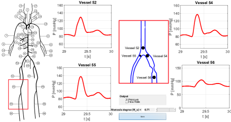
Figure 1: This figure shows an arterial network consisting of the $55$ main arteries of the systemic circulation [65, 73, 76]. In Vessel $54$ (right anterior tibial artery) we put a stenosis and study the effect on blood flow. The stenosis splits Vessel $54$ into two parts. The proximal part is again labelled with the index $54$, while the distal part receives the index $56$. At the places of the black dots that are located at the outlet of Vessel $52$, at the inlets of Vessel $54$ and Vessel $55$ as well as at the inlet of Vessel $56$, we report over one heart beat pressure and flow rate curves. Samples of these curves serve as training data for the kernel methods creating a surrogate model which maps the degree of stenosis $R_{s}\in\left[0,1\right]$ to the samples of the corresponding curves.

2.1 Modelling of blood flow through a single vessel

Let us suppose that the Navier-Stokes equations are defined on cylindrical domains of length $l_{i}\in\mathbb{R},\;i\in\left\{1,\ldots,55\right\}$ and that their main axis are aligned with the $z$-coordinate. Modelling the viscous forces, we assume that blood in large and medium sized arteries can be treated as an incompressible Newtonian fluid, since blood viscosity is almost constant within large and middle sized vessels [49]. The boundaries of the computational domain change in time due to the elasticity of the arterial vessels walls and the pulsatile flow. Thereby, it is assumed that the vessel displaces only in the radial direction and that the flow is symmetric with respect to the main axis of the vessel [21, 50]. In addition to that we postulate that the $z$-component $\mathbf{u}_{z}$ of the velocity flield $\mathbf{u}$ is dominant with respect to the other components. Taking all these assumptions into account and integrating the Navier-Stokes equations across a section area $S\left(z,t\right)$ perpendicular to the $z$-axis at the place $z\in\left(0,l_{i}\right)$ and a time $t>0$, one obtains the following system of PDEs [7, 9, 30]:

$$\frac{\partial A_{i}}{\partial t}+\frac{\partial Q_{i}}{\partial z}=0, \;z\in\left(0,l_{i}\right),\;t>0,$$ (1)

$$\frac{\partial Q_{i}}{\partial t}+\frac{\partial}{\partial z}\left(\frac{Q_{i}^{2}}{A_{i}}\right)+\frac{A_{i}}{\rho}\frac{\partial p_{i}}{\partial z}=-K_{r}\frac{Q_{i}}{A_{i}}, \;z\in\left(0,l_{i}\right),\;t>0.$$ (2)

The unknowns of this system $A_{i}$, $Q_{i}$ and $p_{i}$ denote the section area of vessel $V_{i}$, the flow rate and the averaged pressure within this vessel. Mathematically, these quantities are defined by the following integrals:

$$A_{i}\left(z,t\right)=\int_{S\left(z,t\right)}\;dS,\quad Q_{i}\left(z,t\right)=\int_{S\left(z,t\right)}\mathbf{u}_{z}\;dS,\quad p_{i}\left(z,t\right)=\frac{1}{A_{i}}\int_{S\left(z,t\right)}P_{i}\;dS,$$

where $P_{i}$ is the 3-D pressure field. Please note that (1) is the 1-D version of the mass conservation equation, while (2) represents the 1-D version of the momentum equations. $\rho$ stands for the density of blood. $K_{r}$ is a resistance parameter containing the dynamic viscosity $\eta$ of blood [67]: $K_{r}=22\pi\eta/\rho$. The PDE system (1) and (2) is closed by means of an algebraic equation, which can be derived from the Young-Laplace equation [46]:

$$p_{i}(z,t)=G_{0,i}\left(\sqrt{\frac{A_{i}}{A_{0,i}}}-1\right),\quad G_{0,i}=\frac{\sqrt{\pi}\cdot h_{0,i}\cdot E_{i}}{\left(1-\nu^{2}\right)\cdot\sqrt{A_{0,i}}},$$ (3)

where $E_{i}$ is the Young modulus, $A_{0,i}$ stands for the section area at rest, $h_{0,i}$ is the vessel thickness and $\nu$ is the Poisson ratio. Due to the fact that biological tissue is practically incompressible, $\nu$ is chosen as follows: $\nu=0.5$. Equation (3) assumes that the vessel wall is instantaneously in equilibrium with the forces acting on it. Effects like wall inertia and viscoelasticity could be incorporated using a differential pressure law [15, 44, 72]. However, neglecting the viscoelasticity, maintains the strict hyperbolicity of the above PDE system [1]. Therefore, the interaction between the blood flow and the elastic vessel walls (3) is accounted for by using (3). Assuming that $G_{0,i}$ and $A_{0,i}$ are constant, the PDE-system (1)-(3) can be represented in a compact form:

$$\frac{\partial\mathbf{U}_{i}}{\partial t}+\frac{\partial\mathbf{F}_{i}}{\partial z}\left(\mathbf{U}_{i}\right)=\mathbf{S}_{i}\left(\mathbf{U}_{i}\right),\;z\in\left(0,l_{i}\right),\;t>0.$$ (4)

For $\mathbf{U}_{i}=\left(A_{i},Q_{i}\right)^{T}$, the flux function $\mathbf{F}_{i}$ and the source function $\mathbf{S}_{i}$ are given by:

$$\mathbf{F}_{i}\left(\mathbf{U}_{i}\right)=\begin{pmatrix}Q_{i}\\ \frac{Q_{i}^{2}}{A_{i}}+\frac{A_{i}^{\frac{3}{2}}}{\rho\sqrt{A_{i,0}}}\end{pmatrix}\;\text{ and }\;\mathbf{S}_{i}\left(\mathbf{U}_{i}\right)=\begin{pmatrix}0\\ -K_{r,i}\frac{Q_{i}}{A_{i}}\end{pmatrix}.$$

This system may be written in a quasilinear form:

$$\frac{\partial\mathbf{U}_{i}}{\partial t}+\nabla_{\mathbf{U}_{i}}\mathbf{F}_{i}\frac{\partial\mathbf{U}_{i}}{\partial z}=\mathbf{S}_{i}\left(\mathbf{U}_{i}\right),\;z\in\left(0,l_{i}\right),\;t>0,$$

where $\nabla_{\mathbf{U}_{i}}\mathbf{F}_{i}$ is the $2\times 2$ Jacobian matrix of the flux function $\mathbf{F}_{i}$, having the eigenvalues $\lambda_{i,1}$ and $\lambda_{i,2}$. Denoting by $v_{i}=Q_{i}/A_{i}$ the fluid velocity and $v_{c,i}\left(A_{i}\right)$ the characteristic wave velocity of vessel $V_{i}$, it can be shown that: $\lambda_{i,1}=v_{i}-v_{c,i}$ and $\lambda_{i,2}=v_{i}+v_{c,i}$. Under physiological conditions, it can be observed that [22]:

$$v_{i}=\frac{Q_{i}}{A_{i}}\ll\sqrt{\frac{G_{0,i}}{2\rho}\sqrt{\frac{A_{i}}{A_{0,i}}}}=v_{c,i}\left(A_{i}\right).$$ (5)

Therefore it holds for the eigenvalues: $\lambda_{i,1}<0$ and $\lambda_{i,2}>0$ and the above PDE-system is hyperbolic. Exploiting the fact that the Jacobian matrix $\nabla_{\mathbf{U}_{i}}\mathbf{F}_{i}$ is diagonalisable, there is an invertible matrix $L_{i}$ such that it can be decomposed as follows: $\nabla_{\mathbf{U}_{i}}\mathbf{F}_{i}=L_{i}^{-1}\Lambda_{i}L_{i}$, where $\Lambda_{i}$ is a diagonal matrix that has the eigenvalues $\lambda_{i,1}$ and $\lambda_{i,2}$ on its diagonal. By this, the PDE-system (4) can written in its characteristic variables $\mathbf{W}_{i}=\left(W_{1,i},W_{2,i}\right)^{T}$:

$$\frac{\partial\mathbf{W}_{i}}{\partial t}+\Lambda_{i}\frac{\partial\mathbf{W}_{i}}{\partial z}=L_{i}\mathbf{S}_{i}\left(\mathbf{W}_{i}\right),\;z\in\left(0,l_{i}\right),\;t>0.$$ (6)

The characteristic variables $\mathbf{W}_{i}$ and $L_{i}$ are related by the following equation:

$$\frac{\partial\mathbf{W}_{i}}{\partial\mathbf{U}_{i}}=L_{i},\;\mathbf{W}_{i}(\mathbf{U}_{i})=\begin{pmatrix}0\\ 0\end{pmatrix}\;\text{ for }\;\mathbf{U}_{i}=\begin{pmatrix}A_{0,i}\\ 0\end{pmatrix}.$$ (7)

An integration of (7) yields that the characteristic variables $W_{1,i}$ and $W_{2,i}$ can be expressed by the primary variables $A_{i}$ and $Q_{i}$ as follows:

$$W_{1,i} =-\frac{Q_{i}}{A_{i}}+4\sqrt{\frac{G_{0,i}}{2\rho}}\left(\left(\frac{A_{i}}{A_{0,i}}\right)^{\frac{1}{4}}-1\right)=-v_{i}+4\cdot\left(v_{c,i}\left(A_{i}\right)-v_{c,i}\left(A_{0,i}\right)\right),$$ (8)

$$W_{2,i} =\frac{Q_{i}}{A_{i}}+4\sqrt{\frac{G_{0,i}}{2\rho}}\left(\left(\frac{A_{i}}{A_{0,i}}\right)^{\frac{1}{4}}-1\right)=v_{i}+4\cdot\left(v_{c,i}\left(A_{i}\right)-v_{c,i}\left(A_{0,i}\right)\right).$$ (9)

Based on condition (5) and the signs of $\lambda_{1,i}$ and $\lambda_{2,i}$, one can prove that $W_{1,i}$ is a backward and $W_{2,i}$ is a forward travelling wave [9] [13, Chap. 2]. Furthermore, it can be shown that $W_{1,i}$ and $W_{2,i}$ are moving on characteristic curves $c_{j,i}$ defined by two ODEs:

$$\frac{dc_{j,i}}{dt}\left(t\right)=\lambda_{j}\left(c_{j,i}(t),t\right),\;j\in\left\{1,2\right\}.$$ (10)

These insights are crucial for a consistent coupling of the submodels at the different interfaces, since it reveals that at each inlet and outlet of a vessel exactly one coupling or boundary condition has to be imposed. The other condition is obtained from the outgoing characteristic variable. At the inlet $z=0$, the variable $W_{1,i}$ is leaving the computational domain, whereas at $z=l_{i}$ the variable $W_{2,i}$ is the outgoing characteristic variable.

2.2 Numerical solution techniques

According to standard literature [54, Chap. 13], the main difficulties that arise in terms of numerical treatment of hyperbolic PDEs are to minimise dissipation and dispersion errors, in order to avoid an excessive loss of mass and a phase shift for the travelling waves. A standard remedy for these problems is to apply higher order discretisation methods in both space and time [65] such that the numerical solution is as accurate as possible. However, higher order discretisation methods tend to create oscillations in the vicinity of steep gradients or sharp corners, which can be removed by some additional postprocessing [24, 35, 36]. Moreover, time stepping methods of higher order require small time steps to be able to resolve the dynamics of a fast and convection dominated flow and to fulfill a CFL-condition, if they are explicit.

Considering all these features, we use in this work the numerical method of characteristics (NMC), which is explicit and of low approximation order (first order in space and time [1, Theorem 1]), leading to large dissipation and dispersion errors. This drawback can be circumvented by using a fine grid in space and sufficiently small timesteps. Since we deal in this work with 1-D problems, a fine grid in space is affordable with respect to computational effort. On the other hand, a fine grid might force an explicit method to exert very small time steps. However, for the NMC it can be proven that its time stepsize is not restricted by a condition of CFL type [1, Prop. 2]. This means that the NMC can use a fine grid in space and time stepsizes that are small enough to capture the convection dominated blood flow and large enough to have an acceptable number of timesteps.

Let us suppose now that the interval $\left[0,l_{i}\right]$ for Vessel $V_{i}$ is discretised by a grid having a meshsize $\Delta z_{i}$ and grid nodes $z_{i,k}=k\cdot\Delta z_{i}\in\left[0,l_{i}\right],\;k\in\left\{0,\ldots,N_{h,i}\right\}$. Here, $N_{h,i}$ is the index of the last grid node. In a time step $\left[t_{n},t_{n}+\Delta t\right]$, the NMC iterates over all the grid nodes. At each grid node $z_{i,k}$ there are two characteristic curves $c_{1,i}^{(k)}$ and $c_{2,i}^{(k)}$ for $W_{1,i}$ and $W_{2,i}$ (see Figure 2). Both curves are linearized in $z_{i,k}$ and $t_{n+1}=t_{n}+\Delta t$. In a next step, the resulting tangents are traced back to the previous time point $t_{n}$, where the corresponding intersection points are denoted by $g_{1,i}^{(k)}$ and $g_{2,i}^{(k)}$, respectively (see Figure 2).

This procedure is equivalent to solving for every $z_{i,k}$ the final value problem [1][Equation (22)], which can be derived from (10):

$$\frac{dc_{j,i}\left(z_{i},t_{n+1},t\right)}{dt}\ =\lambda_{j}\left(c_{j,i}\left(z_{i},t_{n+1},t\right),t\right),\;c_{j,i}\left(z_{i},t_{n+1},t_{n+1}\right)=z_{i,k},\;j\in\left\{1,2\right\}.$$

Setting $c_{j,i}\left(z_{i},t_{n+1},t_{n}\right)=g_{j,i}^{(k)}$ we have by a first order approximation:

$$c_{j,i}\left(z_{i},t_{n+1},t_{n+1}\right)-c_{j,i}\left(z_{i},t_{n+1},t_{n}\right) =\int_{t_{n}}^{t_{n+1}}\lambda_{j}\left(c_{j,i}\left(z_{i},t_{n+1},t\right),t\right)\;dt,$$

$$z_{i,k}-g_{j,i}^{(k)}\left(t_{n}\right) =\int_{t_{n}}^{t_{n+1}}\lambda_{j}\left(c_{j,i}\left(z_{i},t_{n+1},t\right),t\right)\;dt$$

$$\approx\Delta t\lambda_{j}\left(c_{j,i}\left(z_{i},t_{n+1},t_{n}\right),t_{n}\right)$$

$$=\Delta t\lambda_{j}\left(g_{j,i}^{(k)}\left(t_{n}\right),t_{n}\right).$$

Restricting the PDE-system (6) to the characteristic curves $c_{j,i}^{(k)}$, we have to solve the following ODEs in order to determine approximations for $W_{1,i}$ and $W_{2,i}$:

$$\frac{d}{dt}\mathbf{W}_{j,i}\left(c_{j,i}^{(k)}(t),t\right)=L_{i}\mathbf{S}_{i}\left(\mathbf{W}_{j,i}\left(c_{j,i}^{(k)}(t),t\right)\right).$$ (11)

An explicit first order discretisation of (11) yields the following extrapolation formula for $\mathbf{W}_{j,i}$ at $c_{j,i}^{(k)}\left(t_{n+1}\right)=z_{i,k}$:

$$\mathbf{W}_{j,i}\left(z_{i,k},t_{n+1}\right)=\mathbf{W}_{j,i}\left(g_{j,i}^{(k)}\left(t_{n}\right),t_{n}\right)+\Delta t\cdot L_{i}\mathbf{S}_{i}\left(\mathbf{W}_{j,i}\left(g_{j,i}^{(k)}\left(t_{n}\right),t_{n}\right)\right).$$ (12)

At the old time step $t_{n}$, the values $\mathbf{W}_{j,i}\left(g_{j,i}^{(k)}\left(t_{n}\right),t_{n}\right)$ can be interpolated using the precomputed values at the grid nodes $z_{i,k}$. For large time steps, it may happen that $g_{j,i}^{(k)}\left(t_{n}\right)\notin\left[0,l_{i}\right]$ (see Figure 2).

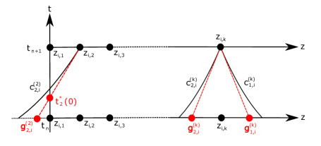
Figure 2: Linearisation of the characteristic curves $c_{j,i}^{(k)}$ for grid nodes $z_{i,k}$ in the vicinity of the boundary and in the inner of the computational domain.

In these cases, the values $\mathbf{W}_{j,i}\left(g_{j,i}^{(k)}\left(t_{n}\right),t_{n}\right)$ can not be interpolated from the spatial values. Therefore, we require a temporal interpolation at a time point at which the linearised characteristic curves leave the computational domain. At the boundaries $z_{i}=0$ and $z_{i}=l_{i}$ these time points $\left\{t^{\ast}_{k}\left(0\right),t^{\ast}_{k}\left(l_{i}\right)\right\}\subset\left[t_{n},t_{n+1}\right]$ can be computed by:

$$t^{\ast}_{k}\left(0\right)=t_{n}-\Delta t\frac{g_{2,i}^{(k)}}{z_{i,k}-g_{2,i}^{(k)}}\;\text{ and }\;t^{\ast}_{k}\left(l_{i}\right)=t_{n}+\Delta t\frac{l_{i}-g_{1,i}^{(k)}}{z_{i,k}-g_{1,i}^{(k)}}.$$

After computing the ingoing characteristic variables $\mathbf{W}_{2,i}\left(0,t_{n+1}\right)$ and $\mathbf{W}_{1,i}\left(l_{i},t_{n+1}\right)$ for the new time step by means of an external model (see Subsection 2.3-2.6), we use a linear interpolation to provide a surrogate value for the missing characteristic variable:

$$\mathbf{W}_{2,i}\left(0,t^{\ast}_{k}\left(0\right)\right) =\frac{t_{n+1}-t^{\ast}_{k}\left(0\right)}{\Delta t}\mathbf{W}_{2,i}\left(0,t_{n}\right)+\frac{t^{\ast}_{k}\left(0\right)-t_{n}}{\Delta t}\mathbf{W}_{2,i}\left(0,t_{n+1}\right),$$

$$\mathbf{W}_{1,i}\left(l_{i},t^{\ast}_{k}\left(l_{i}\right)\right) =\frac{t_{n+1}-t^{\ast}_{k}\left(l_{i}\right)}{\Delta t}\mathbf{W}_{1,i}\left(l_{i},t_{n}\right)+\frac{t^{\ast}_{k}\left(l_{i}\right)-t_{n}}{\Delta t}\mathbf{W}_{1,i}\left(l_{i},t_{n+1}\right).$$ (13)

2.3 Modelling of heart beats

At the inlet of the aorta, we couple the corresponding 1-D model with a lumped parameter model (0-D model) for the left ventricle of the heart. By means of this model and the outgoing characteristic variable $W_{1,1}$ the missing ingoing variable $W_{2,1}$ can be determined. In order to compute the pressure $P_{LV}$ in the left ventricle, we consider the following elastance model [21, 38]:

$$P_{LV}(t)=E(t)\left(V(t)-V_{0}\right)+S(t)Q_{LV}(t),\;\frac{dV}{dt}=-Q_{LV}(t),$$ (14)

where $V$ is the volume of the left ventricle and $Q_{LV}$ is the flow rate from the left ventricle into the aorta. $V_{0}$ is the dead volume of the left ventricle and $S$ denotes the viscoelasticity coefficient of the cardiac wall. For simplicity, we assume that $S$ depends linearly on $P_{LV}$: $S(t)=5.0\cdot 10^{-4}\cdot P_{LV}(t)$. The time dependent elasticity parameter $E$ is given by [38]:

$$E(t)=E_{max}\cdot e_{v}(t)+E_{min},$$

$$\;e_{v}(t)=\begin{cases}0.5\left(1.0-\cos\left(\frac{\pi t}{T_{vcp}}\right)\right),\;0\leq t\leq T_{vcp},\\ 0.5\left(1.0-\cos\left(\frac{\pi\left(t-T_{vcp}\right)}{T_{vrp}}\right)\right),\;T_{vcp}\leq t\leq T_{vcp}+T_{vrp},\\ 0.0,\;T_{vcp}+T_{vrp}<t\leq T.\end{cases}$$

$T$ represents the length of the heart cycle. $E_{max}$ and $E_{min}$ are the maximal and minimal elasticity parameters, while $T_{vcp}$ and $T_{vrp}$ refer to the durations of the ventricular contraction and relaxation. The flow rate $Q_{LV}$ through the aortic valve is governed by the Bernoulli law [69] incorporating the viscous resistance and inertia of blood:

$$L\frac{dQ_{LV}}{dt}=\Delta P_{v}(t)-R\cdot Q_{LV}(t)-B\cdot Q_{LV}(t)\cdot\left|Q_{LV}(t)\right|.$$ (15)

The parameters $R,\;B$ and $L$ quantify the viscous effects, flow separation and inertial effects. Finally, the pressure drop $\Delta P_{v}(t)$ is computed as follows: $\Delta P_{v}(t)=P_{LV}(t)-p_{1}(0,t),\;t>0$, where $p_{1}\left(0,t\right)$ is the pressure at the root of the aorta.

During the systolic phase of the heart cycle, it holds: $\Delta P_{v}(t)>0$ and we use (14)–(15) to compute $Q_{LV}(t)$. This value serves as a Dirichlet boundary value at $z_{1}=0$ for the 1-D model in vessel $V_{1}$. Based on $Q_{LV}(t)$, Equation (8) and (9) and an approximation of $W_{1,1}\left(0,t\right)$ by (12) the ingoing variable $W_{2,1}\left(0,t\right)$ can be determined.

Within the diastolic phase of the heart cycle, $p_{1}(0,t)$ begins to exceed the pressure in the left ventricle $P_{LV}(t)$. As a result the aortic valve is closing and we have no flux or a very little flux between the left ventricle and the aorta and therefore we set $Q_{LV}(t)=0$. Since we simulate only the left ventricle without taking into account the filling process by the left atrium, we reactivate the model at the begin of every heart cycle [21]. Thereby, at the end of each heart cycle, the volume of the left ventricle is set to its maximal value: $V\left(k\cdot T\right)=V_{max},\;k\in\mathbb{N}$.

2.4 Modelling of bifurcations

In order to decrease the flow velocity and to cover the whole body with blood vessels, the arterial system exhibits several levels of branchings. Therefore, it is very important to simulate blood flow through a bifurcation as exact as possible. Bifurcations and their mathematical modelling have been the subject of many publications [10, 20, 29, 35, 66]. Coupling conditions for systems linked at a bifurcation can be derived by the principles of mass conservation and continuity of the total pressure. The total pressure for Vessel $V_{i}$ is defined by:

$$p_{t,i}=\frac{\rho}{2}\left(\frac{Q_{i}}{A_{i}}\right)^{2}+p\left(A_{i}\right).$$

Indexing the vessels at a bifurcation by $V_{i},\;i\in\left\{\text{I},\text{II},\text{III}\right\}\subset\left\{1,\ldots,55\right\}$, we obtain the following three coupling conditions:

$$Q_{\text{I}}=Q_{\text{II}}+Q_{\text{III}}\quad\text{ and }\quad p_{t,\text{I}}=p_{t,\text{II}},\quad p_{t,\text{I}}=p_{t,\text{III}}.$$ (16)

The remaining equations are obtained by the characteristics entering the bifurcation (see Figure 3). According to Subsection 2.1 we have at each bifurcation three characteristics moving from the vessels into the bifurcation. The outgoing characteristic variables can be determined by tracing back the corresponding characteristic curves (see Subsection 2.2, Equation (12) and (2.2)). Using the characteristic variables and inserting (8) and (9) into (16), we obtain a non-linear system of equations for the three unknown ingoing characteristic variables $W_{1,\text{I}}$, $W_{2,\text{II}}$ and $W_{2,\text{III}}$.

Figure 3: Decomposition of a bifurcation into three independent vessels $V_{\text{I}}$, $V_{\text{II}}$ and $V_{\text{III}}$. Orientating the axes of the vessels as in the figure, the characteristic variables $W_{2,\text{I}}$, $W_{1,\text{II}}$ and $W_{1,\text{III}}$ are leaving the corresponding vessels. These variables can be determined by values from the inside of the vessels and combined with the coupling conditions (16), we have a system of equations yielding the boundary values for $V_{\text{I}}$, $V_{\text{II}}$ and $V_{\text{III}}$.

2.5 Modelling of the peripheral circulation

At the outlet of a terminal vessel $V_{i}$, the reflections of the pulse waves at the subsequent vessels have to be incorporated to simulate a realistic pressure decay. For this purpose we assign to each terminal vessel a reflection parameter $R_{p,i}=R_{1,i}+R_{2,i}$, where $R_{1,i}$ is the resistance parameter of $V_{i}$ and $R_{2,i}$ is the equivalent resistance parameter for all the vessels which are connected to $V_{i}$ but not contained in the 1-D network. A third parameter $C_{i}$ quantifies the compliance of the omitted vessels and, therefore, it is a measure for the ability of these vessels to store a certain blood volume. These parameters form a triple $\left(R_{1,i},C_{i},R_{2,i}\right)$ that is referred to as a three-element Windkessel model in literature [4] [23, Chap. 10]. In order to describe the dynamics of a Windkessel model the following ODE has been derived using averaging techniques and an analogy from electrical science [3, 4, 41]:

$$p_{i,t}+R_{2,i}C_{i}\frac{dp_{i,t}}{dt}=p_{v}+\left(R_{1,i}+R_{2,i}\right)Q_{i,t}+R_{1,i}R_{2,i}C_{i}\frac{dQ_{i,t}}{dt}.$$ (17)

$p_{i,t}=p\left(A_{i}\right)$ and $Q_{i,t}$ denote the pressure and flow rate at the outlet $z=l_{i}$ of a terminal vessel $V_{i}$, respectively. $p_{v}$ is an averaged pressure in the venous system. Combining (17) with (3), (8) and (9) yields an equation depending on the characteristic variables. By means of this equation and the given outgoing characteristic variable $W_{2,i}$, the missing ingoing characteristic variable $W_{1,i}$ can be computed, by solving for each time point of interest a non-linear equation. Having $W_{1,i}$ and $W_{2,i}$ at $z=l_{i}$ and for a time point $t>0$ at hand, the boundary values $A_{i}\left(l_{i},t\right)$ and $Q_{i}\left(l_{i},t\right)$ can be computed for each $t>0$ using (8) and (9). Further information on the derivation of lumped parameter models for the peripheral circulation can be found in [47].

2.6 Modelling the influence of a stenosis on blood flow

A blood vessel $V_{i}$ containing a stenosis is split into three parts: A proximal part $V_{i,p}$, the stenosis itself and a distal part $V_{i,d}$. In a next step, we assign to $V_{i,p}$ and $V_{i,d}$ the 1-D blood flow model from Subsection 2.1, while the part of $V_{i}$ that is covered by the stenosis is lumped to a node (see Figure 4).

Figure 4: Decomposition of a blood vessel $V_{i}$ into a proximal part $V_{i,p}$ and a distal part $V_{i,d}$. The stenosis having a degree of stenosis $R_{s}\in\left[0,1\right]$ is lumped to a node and modelled by a $0$-D model. In order to provide boundary conditions at $z=l_{i,p}$ and $z=0$ for the $1$-D models accounting for the influence of the stenosis, the outgoing characteristics $W_{2,i,p}$ and $W_{1,i,d}$ are combined with the coupling conditions of the $0$-D model.

The degree of stenosis is represented by a parameter $R_{s}\in\left[0,1\right]$, where $R_{s}=0$ corresponds to the healthy state and $R_{s}=1$ stands for the case of a completely occluded blood vessel. For convenience, it is assumed that both vessel parts have the same section area $A_{0,i}$ as well as the same elasticity parameters. The lengths of $V_{i,p}$ and $V_{i,d}$ are denoted by $l_{i,p}$ and $l_{i,d}$. At the boundaries $z_{i,p}=l_{i,p}$ and $z_{i,d}=0$ that are adjacent to the stenosis, two characteristic variables $W_{2,i,p}$ and $W_{1,i,d}$ are moving towards the stenosis (see Figure 4 and Subsection 2.1). Using these characteristic variables and an appropriate $0$-D model, we have enough equations to compute the boundary conditions for the two 1-D models. Modelling the stenosis, we consider an ODE containing several parameters of physical relevance to couple both parts of the affected vessels. According to [64, 68, 79] the flow rate $Q_{s}$ through a stenosis and the pressure drop $\Delta p_{s}\left(t\right)=p_{i,d}\left(0,t\right)-p_{i,p}\left(l_{i,p},t\right)$ across a stenosis are related to each other by the following ODE:

$$\frac{K_{u}\cdot\rho\cdot l_{s}}{A_{0,s}}\frac{dQ_{s}}{dt}=\Delta p_{s}-\frac{K_{v}\cdot\eta\cdot l_{s}}{A_{0,s}\cdot D_{s}}Q_{s}-\frac{K_{t}\cdot\rho}{2A_{0,s}^{2}}\left(\frac{A_{0,s}}{A_{s}}-1\right)^{2}Q_{s}\left|Q_{s}\right|.$$ (18)

$A_{0,s}$ and $A_{s}=\left(1-R_{s}\right)\cdot A_{0,s}$ refer to the section areas of the normal and stenotic segments, while $D_{0}$ and $D_{s}$ denote the corresponding diameters [38]. $l_{s}$ is the length of the stenosis. The remaining parameters are empirical coefficients, which are given by [38]:

$$K_{v}=32.0\cdot\left(0.83\cdot l_{s}+1.64\cdot D_{s}\right)\cdot\left(\frac{A_{0,s}}{A_{s}}\right)^{2}\frac{1}{D_{s}},\;K_{t}=1.52\;\text{ and }\;K_{u}=1.2.$$

Solving (18), we use the solution value $Q_{s}$ for each time point as a boundary condition at $z_{i,p}=l_{i,p}$ and $z_{i,d}=0$. Together with the extrapolated characteristic variables $W_{2,i,p}$ and $W_{1,i,d}$ as well as (8) and (9), we have a system of equations for the boundary conditions adjacent to the stenosis.

In the case of a full occlusion, i.e. $R_{s}=1$, we multiply (18) by $A_{s}^{2}$. Considering the limit $A_{s}\rightarrow 0$, we obtain an algebraic equation that gives $Q_{s}=0$. This is equivalent to a full reflection of the ingoing characteristics $W_{2,i,p}\left(l_{i,p},t\right)$ and $W_{1,i,d}\left(0,t\right),\;\;t>0$.

3 Kernel-based surrogate models

In this section we introduce kernel methods for surrogate modeling. First, we present the general ideas of kernel methods applied to the approximation of an arbitrary continuous function $f:\Omega\subset\mathbb{R}^{d}\to\mathbb{R}^{q}$, where $\Omega$ is a given input parameter domain and $d,q$ are the input and output dimensions, which can be potentially large (e.g., the present setting will lead to $q=400$). Then we concentrate on the present field of application and discuss how this general method can be used to produce cheap surrogates of the full model described in the previous sections.

Our goal is to construct a surrogate function ${\hat{f}}:\Omega\to\mathbb{R}^{q}$ such that ${\hat{f}}\approx f$ on $\Omega$, while the evaluation of ${\hat{f}}$ for any input value is considerably cheaper than evaluating $f$ for the same input. This approximation is produced in a data-dependent fashion, i.e., a finite set of snapshots, obtained with the full simulation, is used to train the model to provide a good prediction of the exact result for any possible input in $\Omega$. The computationally demanding construction of the snapshots is performed only once and in an offline phase, while the online computation of the prediction for a new input parameter uses the cheap surrogate model.

3.1 Basic concepts of kernel methods

We introduce here only the basic tools needed for our analysis. For an extensive treatment of kernel-based approximation methods we refer to the monographs [17, 19, 75], while a detailed discussion of kernel-based sparse surrogate models can be found in [28]. Nevertheless, we recall that this technique has several advantages over other approximation methods, namely it allows for large input and output dimensions, it works with scattered data, it allows fast and sparse solutions through greedy methods and has a notable flexibility related to the choice of the particular kernel.

As recalled before, we aim at the reconstruction of a function $f:\Omega\to\mathbb{R}^{q}$, $\Omega\subset\mathbb{R}^{d}$. We assume to have a dataset given by $N\in\mathbb{N}$ pairwise distinct inputs, i.e., a set $X_{N}:=\{x_{1},\dots,x_{N}\}\subset\Omega$ of $N$ points in $\Omega$ (the data points) and corresponding function evaluations $F_{N}:=\{f(x_{i}),x_{i}\in X_{N}\}\subset\mathbb{R}^{q}$ (the data values).

The construction of ${\hat{f}}$ makes use of a positive definite kernel $K$ on $\Omega$. We recall that a function $K:\Omega\times\Omega\to\mathbb{R}$ is a strictly positive kernel on $\Omega$ if it is symmetric and, for any $N\in\mathbb{N}$ and any set of pairwise distinct points $X_{N}:=\{x_{1},\dots,x_{N}\}\subset\Omega$, the $N\times N$ kernel matrix $A_{K,X_{N}}:=(K(x_{i},x_{j}))_{i,j=1}^{N}$ is positive definite. Many strictly positive definite kernels are known in explicit form, and notable examples are e.g. the Gaussian $K(x,y):=\exp(-\varepsilon^{2}\|x-y\|_{2}^{2})$ (where $\varepsilon$ is a tunable parameter) and the Wendland kernels [74], which are radial and compactly supported kernels of piecewise polynomial type and of finite smoothness. Given a kernel $K$, the surrogate model ${\hat{f}}:\Omega\to\mathbb{R}^{q}$ is constructed via the ansatz

$${\hat{f}}(x):=\sum_{j=1}^{N}\alpha_{j}K(x,x_{j}),\;x\in\Omega,$$ (19)

with unknown coefficient vectors $\alpha_{j}\in\mathbb{R}^{q}$. The coefficients are obtained by the vectorial interpolation conditions

$${\hat{f}}(x_{i})=f(x_{i}),\;1\leq i\leq N,$$ (20)

i.e., the surrogate model ${\hat{f}}$ is required to predict the same value of the full model $f$ when computed on each of the data points contained in the dataset. Putting together the ansatz (19) and the interpolation conditions (20), one obtains the set of equations

$${\hat{f}}(x_{i})=\sum_{j=1}^{N}\alpha_{j}K(x_{i},x_{j})=f(x_{i}),\;1\leq i\leq N,$$

which can be formulated as a linear system $A_{K,X_{N}}\alpha=b$ with

$$A_{K,X_{N}}:=[K(x_{i},x_{j})]_{i,j=1}^{N}\in\mathbb{R}^{N\times N},\;\alpha:=\left[\begin{array}[]{c}\vdots\\ \alpha_{j}^{T}\\ \vdots\\ \end{array}\right]\in\mathbb{R}^{N\times q},\;b:=\left[\begin{array}[]{c}\vdots\\ f(x_{i})^{T}\\ \vdots\\ \end{array}\right]\in\mathbb{R}^{N\times q}.$$ (21)

Since the kernel is chosen to be strictly positive definite, the matrix $A_{K,X_{N}}$ is positive definite for any $X_{N}$, thus the above linear system possesses a unique solution $\alpha\in\mathbb{R}^{N\times q}$. In other terms, the model (19) satisfying interpolation conditions (20) is uniquely defined for arbitrary pairwise distinct data points $X_{N}$ and data values $F_{N}$.

This interpolation scheme can be generalised by introducing a regularisation term, which reduces possible oscillations in the surrogate at the price of a non exact interpolation of the data. We remark that in principle this does not reduce the accuracy, since a parameter $\lambda\geq 0$ can be used to tune the influence of the regularization term, and a zero value can be used when no regularization is needed.

To explain this in details, we first recall that, associated with a strictly positive definite kernel there is a uniquely defined Hilbert space $\mathcal{H}_{K}(\Omega)$ of functions from $\Omega$ to $\mathbb{R}^{q}$. For the sake of simplicity, we discuss the case $q=1$, i.e., scalar valued functions, while the generalisation to vectorial functions will be sketched at the end of this section. The space $\mathcal{H}_{K}(\Omega)$ contains in particular all the functions of the form (19), and their squared norm can be computed as $\|\hat{f}\|^{2}_{\mathcal{H}_{K}(\Omega)}=\alpha^{T}A_{K,X_{N}}\alpha$. This means that a surrogate with small $\mathcal{H}_{K}(\Omega)$-norm is defined by coefficients $\alpha$ with small magnitude.

With these tools, and again for $q=1$ and a regularisation parameter $\lambda\geq 0$, a different surrogate can be defined as the solution of the optimisation problem

$$\min_{{\hat{f}}\in\mathcal{H}_{K}(\Omega)}\sum_{i=1}^{N}\left(f(x_{i})-{\hat{f}}(x_{i})\right)^{2}+\lambda\|{\hat{f}}\|_{\mathcal{H}_{K}(\Omega)}^{2}=\min_{\alpha\in\mathbb{R}^{N}}\|A_{K,X_{N}}\alpha-b\|_{2}^{2}+\lambda\alpha^{T}A_{K,X_{N}}\alpha,$$ (22)

which is a regularised version of the interpolation conditions (20), where exact interpolation is replaced by square error minimization, and the surrogate is requested to have a small norm. When a strictly positive definite kernel is used, the Representer Theorem [61] guarantees that the problem (22) has a unique solution, that this solution is of the form (19), and that the coefficients $\alpha$ are defined as the solutions of the linear system

$$\left(A_{K,X_{N}}+\lambda I\right)\alpha=b,$$

where $I$ is the $N\times N$ identity matrix, and where now $\alpha$ and $b$ are column vectors. It is now clear that pure interpolation can be obtained by letting $\lambda=0$ although a positive $\lambda$ improves the conditioning of the linear system, reducing possible oscillations in the solution.

These Hilbert spaces, the corresponding error analysis, and the formulation of the regularised interpolant can be extended to the case of vector valued functions $f:\Omega\to\mathbb{R}^{q}$ just by applying the same theory to each of the $q$ components. The fundamental point here, to have an effective method to be used in surrogate modeling, is to avoid having $q$ different surrogates, one for each component. This would result in $q$ independent sets of centers, hence many kernel evaluations to compute a point value ${\hat{f}}(x)$. To reduce the overall number of centers, one can make the further assumption that a common set of centers is used for all components. From the point of view of the actual computation of the interpolant, this is precisely equivalent to the solution of the linear system (21), where in the regularised case also the term $\lambda I$ is included. We remark that more sophisticated approaches are possible to treat vector valued functions, but the approach presented in this work yields already satisfactory results.

3.2 Sparse approximation

So far, we have shown that kernel interpolation is well defined for arbitrary data, and that the corresponding interpolant has certain approximation properties. Although the method can deal with arbitrary pairwise distinct inputs $X_{N}$, the resulting surrogate model ${\hat{f}}$ is required to be fast to evaluate. From formula (19), it is clear that the computational cost of the evaluation of ${\hat{f}}(x)$ on a new input parameter $x\in\Omega$ is essentially related to the number $N$ of elements in the sum. It is thus desirable to find a sparse expansion of the form (19), i.e., one where most of the coefficient vectors $\alpha_{j}$ are zero. This sparsity structure can be obtained by selecting a small subset $X_{n}\subset X_{N}$ of the data points, and computing the corresponding surrogate.

An optimal selection of these points is a combinatorial problem, which is too expensive with respect to the computational effort. Instead, we employ greedy methods (see [70] for a general treatment, and [14, 59] for the case of kernel approximation). Such methods select a sequence of data points starting with the empty set $X_{0}:=\emptyset$, and, at iteration $n\geq 1$, they update the set as $X_{n}:=X_{n-1}\cup\{x_{n}\}$ by adding a suitable selected point $x_{n}\in X_{N}\setminus X_{n-1}$. The selection of $x_{n}$ is done here with the $f$-Vectorial Kernel Orthogonal Greedy Algorithm ($f$-VKOGA, [77]), which works as follows. At each iteration, a partial surrogate can be constructed as

$${\hat{f}}_{n}(x)=\sum_{j=1}^{n}\alpha_{j}K(x,x_{j}),\;\;(A_{K,X_{n}}+\lambda I)\alpha=b_{X_{n}},$$

where $A_{K,X_{n}}$, $b_{X_{n}}$ are the matrix and vector of (21) restricted to the points $X_{n}$. To evaluate the quality of the partial surrogate, one can check the residual vector

$$r_{n}(f)(x):=f(x)-{\hat{f}}_{n}(x)$$

for all $x\in X_{N}\setminus X_{n}$. The $f$-VKOGA takes precisely $x_{n}:=\max_{x\in X_{N}\setminus X_{n-1}}\|r_{n}(x)\|_{2}$, i.e., it includes in the model the data point where the error is currently largest. By checking the size of the residual, one can stop the iteration with ${\hat{f}}_{n}\approx{\hat{f}}$, while potentially $n\ll N$, i.e., the new surrogate model is much cheaper to evaluate but it retains the same accuracy of ${\hat{f}}$. More precisely, it has been proven that, under smoothness assumptions on the target function $f$, the VKOGA algorithm, with the $f$- or similar selection strategies, can attain algebraic or even spectral convergence rates [58, 77].

Finally, we remark that the partial surrogates can be efficiently updated when adding a new point, i.e., ${\hat{f}}_{n}$ can be obtained from $\hat{f}_{n-1}$ by computing only a new coefficient in the expansion, while the already computed ones are not modified. We point to the paper [28] for a more in depth explanation of this efficient computational process.

Observe that this greedy method results in the selection of a small subspace $V_{n}:=\mathrm{span}\{K(\cdot,x_{i}),x_{i}\in X_{n}\}$, and $\hat{f}_{n}$ is computed as the projection, thus best approximation, of $f$ into $V_{n}$. The selection of the points $X_{n}$ via the $f$-greedy selection strategy makes use of the values of $f$ on all the points $X_{N}$. In this sense, the procedure is similar to a least square approximation, where a small set of points is used to generate an accordingly small approximation space. Nevertheless, it is not clear in the least square setting how these few points should be selected, whereas the present approach allows an incremental selection of points and an efficient update of the approximant, which can be stopped when a tolerance criterion is reached. Moreover, by solving equation (22) we are indeed constructing an approximant that minimizes a least squares accuracy term combined with a regularization term.

3.3 Simulating blood flow in the vicinity of a peripheral stenosis by means of kernel methods

Coming back to the blood flow simulation, we define in details the target functions $f$ which will be approximated by the kernel method. These functions will represent the maps from an input stenosis degree $R_{s}\in[0,1]$ to the resulting pressure or flow-rate curve for different vessels, as computed by the full simulation of Section 2.2. The definition of $f$ is described in the following.

Since the numerical simulation is expected to have a transient phase before reaching an almost-periodic behaviour, the system is first simulated with the method of Section 2.2 in the time interval $[T_{0}:=0s,T_{1}:=20s]$ for the healthy state $R_{s}=0$. The state reached at time $T_{1}$ is then used as initial value for the subsequent simulations. At the time $T_{1}$ the stenosis is activated with a degree $R_{s}\in[0,1]$ and the system is simulated until $T_{2}=30s$ for various values of $R_{s}$.

From this set of simulations for different values of $R_{s}$, we keep the pressure and flow-rate curves of the last heart beat, i.e., in the time interval $[29s,30s]$. This means that for each point in the spatial grid we have the time evolution of the pressure and flow rate, which are represented as a $q$-dimensional vector for each space point, where $q$ depends on the actual time discretization step.

In order to study the effect of the stenosis, we concentrate on the vessels number $N_{v}\in\{52,54,55,56\}$, which are the ones surrounding the stenosis (see Figure 1), and for each of those we select a reference space point. Putting all together, for each of the four vessels we have one reference point located in the middle of these vessels. For each point we have the $q$-dimensional time discretization of the pressure and flow rate curve in the time interval $[29s,30s]$. The maps from an input stenosis degree to these vectors define functions $f^{P}_{N_{v}}:[0,1]\to\mathbb{R}^{q}$ (for the pressure) and $f^{F}_{N_{v}}:[0,1]\to\mathbb{R}^{q}$ (for the flow rate).

Figure 5 and 6 show examples of pressure and flow rate curves, for both healthy state and for $R_{s}\approx 0.7$. It can be observed that in the case $R_{s}\approx 0.7$ the flow rate in Vessel $54$ and $56$ is remarkably reduced, while the flow rate in Vessel $55$ is slightly enlarged. The pressures in Vessel $52$, $54$ and $55$ are increased, which may lead to the formation of an aneursysm, if the vessel walls are weakend in this region. Concerning the healthy state $R_{s}=0$, one has to note that the pressure values are within a physiological reasonable range, i.e., $79\mathrm{mmHg}$ for the diastolic pressure and $130\mathrm{mmHg}$ for the systolic pressure. Similar pressure curves have also been published in other works [4, 38].

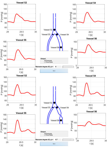
Figure 5: Pressure curves around the stenosis for the healthy state (top) and a degree of stenosis $R_{s}\approx 0.7$ (bottom). The curves are reported at the black dots for $t\in\left[29\mathrm{s},30\mathrm{s}\right]$.

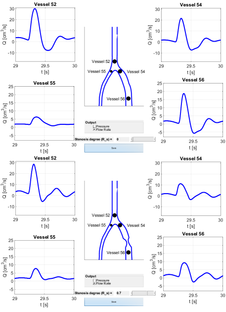
Figure 6: Flow rate curves around the stenosis for the healthy state (top) and a degree of stenosis $R_{s}\approx 0.7$ (bottom). The curves are reported at the black dots for $t\in\left[29\mathrm{s},30\mathrm{s}\right]$.

With respect to the general setting introduced in the previous section, we have here $d:=1$, $q=400$, $\Omega:=[0,1]$. We can then train a kernel model for each of the eight functions (corresponding to pressure and flow-rate for each of the four vessels) using snapshot-based datasets. In particular, the data points $X_{N}\subset[0,1]$ are a set of $N$ pairwise distinct stenosis degrees, and $F_{N}\subset\mathbb{R}^{q}$ is the set of snapshots obtained by the full model run on the input parameters $X_{N}$.

Those models can then be used to predict the output of the simulation for an input stenosis not present in the dataset. For example, for a given value $R_{s}\in[0,1]$, the evaluation $\hat{f}_{N_{v}}^{P}(R_{s})$ is a $q$-dimensional vector which approximates the pressure curve in the time interval $[29s,30s]$ in vessel $N_{v}$ with stenosis degree $R_{s}$. We remark that this setting can be easily modified to approximate different aspects of the full simulation, although the present ones yield interesting insights into the behaviour of the system.

Before we present the numerical tests, two remarks on the data are in order. First, the current time step produces $400$ samples per second, which means that we have $q=400$, i.e., we are approximating functions $\left[0,1\right]\to\mathbb{R}^{400}$. Second, the data obtained with $R_{s}=0$ are removed from the datasets and replaced with the one with $R_{s}=10^{-6}$, since the ODE model (18) is meaningful only for a strictly positive value of the stenosis degree, while the quadratic term vanishes for $R_{s}=0$, thus leading to a different model. This restriction is not relevant from an application point of view, since the a value $R_{s}=10^{-6}$ can be considered to effectively represent the healthy state.

In the training of each model, the parameters $\varepsilon$ and $\lambda$ are chosen within a range of possible values by $k$-fold cross validation. This means that the training data are randomly permuted and divided into $k$ disjoint subsets of approximately the same size and, for each pair $(\varepsilon,\lambda)$ of possible parameters, a model is trained on the union of $k-1$ subsets and tested on the remaining one. This operation is repeated $k$ times changing in all possible ways the $k-1$ sets used for training. The average of the error obtained by these $k$ tests is assigned as the error score of the parameter pair, and the best pair $(\varepsilon,\lambda)$ is chosen as the one yielding the smallest error score. The actual model is then trained on the whole training set using these parameters. In more details, we use here $10$-fold cross validation and test $20$ logarithmic equally spaced values $\varepsilon\in[10^{-2},50]$ and $15$ logarithmic equally spaced values $\lambda\in[10^{-16},10^{-2}]$. The error measure to sort the parameters is the maximum absolute error.

4 Numerical tests

This section is concerned with the training of the surrogate models and analyses them under different perspectives. We train different surrogates using different training sets of increasing size to analyse the number of full model runs needed to have an accurate surrogate. They are obtained each with $N$ equally spaced stenosis degrees in $\left[10^{-6},1\right]$, with $N=\{5,10,20,40,80,160,320,640\}$.

A further dataset of $N=1000$ equally spaced stenosis degrees is used as a test set, i.e., the surrogates computed with the various training datasets are evaluated on this set of input stenosis degrees, and the results are compared with the full model computations. We remark that the values of this test set are not contained in the training sets (except for $R_{s}=10^{-6}$ and $R_{s}=1$), so the results are reliable assessments of the models’ accuracy. For every value $(R_{s})_{i}$ in the test set we consider the absolute and relative errors

$$e_{A}^{(i)}:=\|f((R_{s})_{i})-{\hat{f}}((R_{s})_{i})\|_{2},\;\;e_{R}^{(i)}:=\frac{\|f((R_{s})_{i})-{\hat{f}}((R_{s})_{i})\|_{2}}{\|f((R_{s})_{i})\|_{2}},$$

and, to measure the overall error over the test set, we compute both the maximum absolute and relative error, i.e.,

$$E_{A}:=\max_{1\leq i\leq 1000}e_{A}^{(i)},\;\;E_{R}:=\max_{1\leq i\leq 1000}e_{R}^{(i)}.$$

We use the Gaussian kernel, and the $f$-VKOGA is stopped using a tolerance $5\cdot 10^{-8}$ on the regularized Power Function, which controls the model stability [28].

4.1 Simulation parameters

Before we study the performance of the numerical model, we summarise the simulation parameters in this subsection. For the 1-D arterial network, the data from [65][Tab. 1] have been used. In this table the different lengths $l_{i}$, section areas $A_{0,i}$ and elasticity parameters $\beta_{i}$ can be found. By means of $\beta_{i}$ and $A_{0,i}$, the elasticity parameters $G_{0,i}$ in (3) can be calculated as follows: $G_{0,i}=\beta_{i}\cdot\sqrt{A_{0,i}}$. Please note that Vessel $54$ from the original data set is split into a new Vessel $54$ of length $l_{54}=10.0\;\mathrm{cm}$, the stenosis of length $l_{s}=1.0\;\mathrm{cm}$ and an additional Vessel $56$ of length $l_{56}=21.2\;\mathrm{cm}$ (see Figure 1 and Figure 4). The resistances $R_{p,i}=R_{1,i}+R_{2,i}$ and capacities $C_{i}$ occuring in (17) are listed in [68][Tab. 2], where the resistance $R_{1,i}$ is determined by the characteristic impedance $Z_{i}=\rho\cdot c\left(A_{0,i}\right)/A_{0,i}$ [4]. For $t=0$, we set $A_{i}(z,0)=A_{0,i},\;Q_{i}(z,0)=0$ and $p_{i}(z,0)=0$ in the corresponding vessels. The parameters for the left ventricle model are listed in Table 1. In order to solve the ODEs occuring in Section 2, we use an explicit discretisation of first order.

Table 1: List of the different parameters for the model of the left ventricle [21][Section 4],[38][Tab. 2].

Physical Parameter	sign	value	unit
dead volume left ventricle	$V_{0}$	$10.00$	$\mathrm{cm^{3}}$
maximal volume	$V_{max}$	$130.00$	$\mathrm{cm^{3}}$
duration of heart cycle	$T$	$1.00$	$\mathrm{s}$
duration of ventricular contraction	$T_{vcp}$	$0.30$	$\mathrm{s}$
duration of ventricular relaxation	$T_{vrp}$	$0.15$	$\mathrm{s}$
maximal elastance	$E_{max}$	$2.75$	$\mathrm{mmHg/cm^{3}}$
minimal elastance	$E_{min}$	$0.08$	$\mathrm{mmHg/cm^{3}}$
viscous resistance	$R$	$3.0\cdot 10^{-3}$	$\mathrm{mmHg\cdot s/cm^{3}}$
separation coefficient	$B$	$2.5\cdot 10^{-5}$	$\mathrm{mmHg\cdot s^{2}/cm^{6}}$
inductance coefficient	$L$	$5.0\cdot 10^{-4}$	$\mathrm{mmHg\cdot s^{2}/cm^{3}}$

4.2 Accuracy of the surrogate models

We start by describing in detail the results obtained for Vessel 56, i.e., for the functions $f_{56}^{P}$ and $f_{56}^{F}$. Figure 7 shows the absolute and relative errors $E^{A}$ (left), $E^{R}$ (right) for the two functions. For both the pressure and flow-rate, it is clear that an increase in the dataset size, hence in the number of full model runs, produces significantly more accurate models. The actual magnitude in the absolute errors is different between pressure and flow rate, due to a different magnitude of the output quantities. Nevertheless, the relative errors demonstrate that the pressure curves are better approximated by the kernel models by about two orders of magnitude, for each dataset size. In any case, the models exhibit a converging behaviour towards the full model. Moreover, it should be noted that already a relatively small dataset of $N=160$ stenosis degrees produces good results in both cases. For a better understanding of the error behaviour, we report in Figure 8 the pointwise absolute and relative errors $e_{A}^{(i)},e_{R}^{(i)}$ for pressure (left) and flow rate (right) in the case $N=640$. Observe that the errors are in all cases very oscillating, since each point in the plots represent one value of $e_{A}^{(i)}$ (or $e_{R}^{(i)}$) for a different value of $(R_{s})_{i}$, i.e., it is the $2$-norm of the $400$ dimensional vector $f((R_{s})_{i})-{\hat{f}}((R_{s})_{i})$. Thus, the small oscillations for a single parameter of the surrogate around the exact solution are amplified into the values depicted in the figures.

It is worth noticing that in both cases the magnitude of the exact quantity is decreasing for $R_{s}$ close to one, thus the relative error is magnified for high stenosis degrees. This effect is particularly evident for the flow-rate, where the kernel model has a better absolute accuracy for $R_{s}\approx 1$, but a significantly worse relative accuracy.

We remark that this causes the worse relative error for the flow rate observed in Figure 7. Indeed, the relative error $E_{R}$ for a given size of the training set is computed as the maximum of the relatives error $e_{R}^{(i)}$ for all the values $(R_{s})_{i}$ in the test set. Thus, $E_{R}$ is dominated by the relative error obtained in the region $R_{s}\approx 1$, which is large due to the small magnitude of the flow rate computed by the full model. A different error measure, e.g. the average relative error, would result in a different error decay in Figure 7.

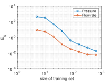
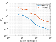
Figure 7: Absolute (left) and relative (right) errors obtained by kernel surrogates with an increasing training set, for both the pressure (blue curves) and flow rate (red curves).

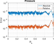
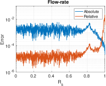
Figure 8: Pointwise absolute (blue) and relative (red) errors obtained by the kernel models with $N=640$ training points for the prediction of the pressure (left) and flow rate (right).

Similar results have been obtained for the other three vessels. The results are reported in Table 2. It is relevant to notice that for these vessels the effect of the stenosis is much less visible. Indeed, the relative error for the flow rate is not significantly worse than the one of the pressure, since the flow does not completely vanish for increasing stenosis degrees. This effect is more evident for the Vessels $52,55$, which are not directly connected with the stenosis.  

Table 2: Accuracy of the surrogates for pressure and flow rate for the Vessels $52,54,55$. The table shows the absolute ($E_{A}$) and relative ($E_{R}$) errors obtained with datasets of increasing size $N$.

Pressure
	Vessel $52$		Vessel $54$		Vessel $55$
$N$	$E_{A}$	$E_{R}$	$E_{A}$	$E_{R}$	$E_{A}$	$E_{R}$
$10$	$5.76\cdot 10^{0}$	$3.01\cdot 10^{-3}$	$7.35\cdot 10^{0}$	$3.80\cdot 10^{-3}$	$7.41\cdot 10^{0}$	$3.85\cdot 10^{-3}$
$40$	$1.15\cdot 10^{0}$	$6.00\cdot 10^{-4}$	$1.50\cdot 10^{0}$	$7.75\cdot 10^{-4}$	$1.51\cdot 10^{0}$	$7.85\cdot 10^{-4}$
$160$	$9.53\cdot 10^{-1}$	$4.97\cdot 10^{-4}$	$1.23\cdot 10^{0}$	$6.35\cdot 10^{-4}$	$1.25\cdot 10^{0}$	$6.47\cdot 10^{-4}$
$640$	$2.95\cdot 10^{-1}$	$1.54\cdot 10^{-4}$	$2.98\cdot 10^{-1}$	$1.54\cdot 10^{-4}$	$3.01\cdot 10^{-1}$	$1.56\cdot 10^{-4}$
Flow rate
$10$	$6.05\cdot 10^{0}$	$3.35\cdot 10^{-2}$	$5.48\cdot 10^{0}$	$2.51\cdot 10^{-1}$	$8.33\cdot 10^{-1}$	$1.20\cdot 10^{-2}$
$40$	$7.72\cdot 10^{-1}$	$4.28\cdot 10^{-3}$	$5.23\cdot 10^{-1}$	$2.41\cdot 10^{-2}$	$1.84\cdot 10^{-1}$	$2.64\cdot 10^{-3}$
$160$	$6.35\cdot 10^{-1}$	$3.52\cdot 10^{-3}$	$4.08\cdot 10^{-1}$	$1.88\cdot 10^{-2}$	$1.41\cdot 10^{-1}$	$2.03\cdot 10^{-3}$
$640$	$1.73\cdot 10^{-1}$	$9.61\cdot 10^{-4}$	$7.70\cdot 10^{-2}$	$3.55\cdot 10^{-3}$	$3.02\cdot 10^{-2}$	$4.34\cdot 10^{-4}$

To further measure the accuracy of the surrogate, we compare a relevant blood flow index obtained with the full model and with the surrogate. We consider the pulsatility index $PI$, which is a commonly used diagnostic index, and has the advantage of being measurable in a non invasive way (see e.g. [68]). For a given stenosis degree $R_{s}$, in vessel $N_{v}$ it is computed as

$$PI^{P}(R_{s}):=\frac{\max\left(f_{N_{v}}^{P}(R_{s})\right)-\min\left(f_{N_{v}}^{P}(R_{s})\right)}{\mathrm{mean}\left(f_{N_{v}}^{P}(R_{s})\right)},\;$$

$$PI^{F}(R_{s}):=\frac{\max\left(f_{N_{v}}^{F}(R_{s})\right)-\min\left(f_{N_{v}}^{F}(R_{s})\right)}{\mathrm{mean}\left(f_{N_{v}}^{F}(R_{s})\right)},$$

for the pressure and flow rate, respectively. It measures the difference between the systolic and diastolic pressure (or flow rate) divided by its average value. This index can be computed in the same way also for the surrogate using the same formula with the full model replaced with the data-based prediction. Figure 9 reports the logarithmic error between the exact and the predicted values of $PI^{P}$ (left) and $PI^{F}$ (right) in Vessel $56$, for all values of $R_{s}$ in the test set, and for the surrogate obtained with $N=640$. The results demonstrate the accuracy of the approximate model also in capturing a physically relevant quantity, and this is obtained by data accuracy only, i.e., no constraint is imposed to the surrogate to match the desired values of the $PI$ index of the full model. The simulation results that are provided in Figure 9 show a similar curve progression as in [68, Figure 3 or Figure 6]. For small stenosis degrees, the normalised $PI$ indices with respect to $R_{s}=0$, i.e. the health state, are almost one. As the stenosis degree increases (see Figures 5 and 6), it can be observed that in particular the systolic pressures and flow rates are damped significantly. As a consequence, the $PI$ indices are decreasing monotonously. Up to a stenosis degree of $R_{s}=0.5$ the gradient of the curve is rather low, while for a severe stenosis $R_{s}>0.5$ the gradient of the $PI$ curve is very high.

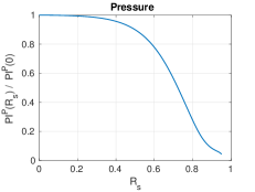
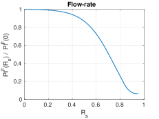
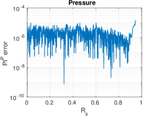
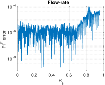
Figure 9: Absolute error between the PI computed with the full model and the one computed with the surrogate for the pressure (top, left) and flow rate (top, right). The results at the bottom line are obtained by a kernel model with $N=640$.

4.3 Efficiency of the surrogate models

It is now of interest to investigate the online efficiency of the surrogates, that is, the time needed to evaluate the models on a new input stenosis. In order to understand the timing results, we remark that the evaluation of the full model for a given stenosis degree $R_{s}$ takes around $t_{full}=200s$, only for the simulation of the time interval [$29s,30s]$, i.e., without considering the transient phase. We remark that the present MATLAB implementation can be significantly optimised for speed, and a smaller execution time can be expected using a compiled language.

Since the $f$-VKOGA constructs the surrogate selecting only a relevant subset of the full dataset, we look at the actual number of points which is selected for the various datasets and output quantities. Figure 10 (left) reports this number of points, as obtained in the approximation of $f^{P}_{56},f^{F}_{56}$ as discussed in the previous section. It is interesting to observe that the number of points increases as the dataset increases, but the number is well below the total number of points. This means that the surrogates are faster than a non-sparse kernel expansion. Moreover, the flow-rate requires the selection of more points, which confirms that this output quantity is more difficult to predict. To assess the actual efficiency of the models, in Figure 10 (right) we report the runtime required to evaluate each model on the $1000$ test stenosis degrees. The evaluation is repeated $100$ times, and the figure shows the mean and standard deviation over the $100$ experiments. As expected, the evaluation times are related to the sparsity of the models.

In all cases the evaluation of the surrogates on $1000$ inputs takes on average less than $1.5\cdot 10^{-2}s$, i.e., for the largest (hence slowest) model we can estimate an evaluation time per stenosis degree to $t_{surrogate}=1.5\cdot 10^{-5}s$. Compared to $t_{full}=2\cdot 10^{2}s$, this still gives a speedup factor of about $10^{6}$ in the worst case.

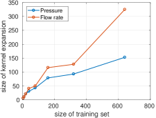
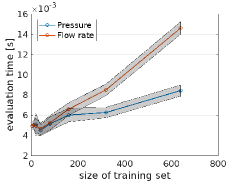
Figure 10: Number of points selected by the $f$-VKOGA (left) and runtime to evaluate the surrogates on $1000$ inputs (right), for Vessel 56 and for datasets of increasing sizes.

4.4 Solving a state estimation problem by means of kernel methods

In order to demonstrate the use of the surrogate model, we employ it to solve a state estimation problem which would be infeasible by using the full model. Namely, for a given pressure or flow rate curve in a time interval, we want to predict as accurately as possible the stenosis degree which corresponds to a given curve. We assume to collect the measurements into a vector $y\in\mathbb{R}^{q}$, which is given by the model output for a fixed, but unknown input stenosis degree $R^{\star}$, plus some additive noise, i.e.,

$$y:=f(R^{\star})+\eta v,$$

where $\eta\geq 0$ is a noise level and $v$ is a random vector. In the following experiments, $v$ is drawn from the uniform distribution in $(0,1)$. We aim at detecting the value $R^{\star}$ from $y$ only. Doing so, we define a cost function $J(R_{s})$ measuring the squared distance between the measurements and the model prediction for a given stenosis degree $R_{s}$, i.e.,

$$J(R_{s}):=\frac{1}{2\|y_{j}\|^{2}_{2}}\sum_{j=1}^{q}\left(y_{j}-\tilde{f}_{j}(R_{s})\right)^{2},$$ (23)

and consider the solution $\tilde{R}^{\star}$ of the optimisation problem

$$\tilde{R}^{\star}=\min_{R_{s}\in[0,1]}J(R_{s}).$$

Observe that, when the noise term $\eta v$ is vanishing and the model prediction is exact, the unique minimiser is the exact solution, i.e., $\tilde{R}^{\star}=R^{\star}$.

In principle, it would be possible to formulate the cost function (23) also in terms of the full model $f$. Nevertheless this is infeasible in practice, since multiple evaluations of $f$ are required to compute a minimiser. The use of the cheap surrogate model, instead, allows a real-time estimation of $R^{\star}$. Moreover, since the kernel is differentiable the cost function is also differentiable, thus the use of gradient-based methods is possible. In particular, we have

$$\frac{d}{dR_{s}}J(R_{s})=\frac{1}{\|y_{j}\|^{2}_{2}}\sum_{j=1}^{q}\left(y_{j}-\tilde{f}_{j}(R_{s})\right)\frac{d}{dR_{s}}f_{j}(R_{s}),$$

with

$$\frac{d}{dR_{s}}f_{j}(R_{s})=\frac{d}{dR_{s}}{\left(\sum_{i=1}^{N}\alpha_{ij}K(R_{s},R_{i})\right)}=\sum_{i=1}^{N}\alpha_{ij}\frac{d}{dR_{s}}K\left(R_{s},R_{i}\right)$$

and the $R_{s}$-derivative of the kernel can be explicitly computed, since the kernel itself is known in closed form. In other terms, both the cost function $J$ and its derivative can be computed efficiently by means of the surrogate, and they both only involve the evaluation of matrix-vector products.

We proceed to some experiments for Vessel 56 and the surrogate models obtained with the dataset of $N=160$ full model runs. In Figure 11, we plot the cost function $J$ for $R_{s}\in[0,1]$ and $R^{\star}=0.1$ (left) and $R^{\star}=0.9$ (right) for the pressure (top) and flow rate (bottom). The results are reported for increasing noise levels $\eta$, obtained as $10$ logarithmically spaced values in $\left[0.01,0.5\right]$. It is clear that the surrogate provides a reliable prediction when the stenosis degree is large, also in the presence of noise, since the cost function has a unique minimiser. Instead, for small target stenosis degrees the cost function is flat, so we should expect a less accurate prediction.

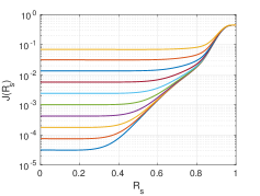
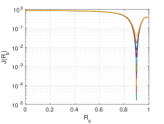
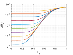
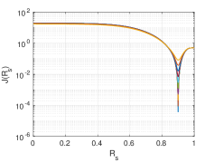
Figure 11: Cost functions $J$ for $R^{\star}=0.1$ (left) and $R^{\star}=0.9$ (right) for the pressure curve (top line) and the flow rate (bottom line), for Vessel 56 and using the surrogate based on the dataset of $N=160$ full model runs. The various curves correspond to increasing noise levels in the target value $y$.

The values of $\tilde{R}^{\star}$ can then be computed with any constrained optimisation solver, and we use here the MATLAB built-in fmincon, which uses an active set search procedure. The noisy input $y$ for $\eta=0.1$, as well as the resulting estimated curves, are depicted in Figure 12, for both $R^{\star}=0.1,0.9$ and both pressure and flow rate. The estimated values $\tilde{R}^{\star}$ are reported in Table 3.

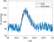
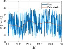
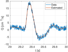
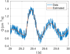
Figure 12: Noisy data and estimated curves for $R^{\star}=0.1$ (left) and $R^{\star}=0.9$ (right) for the pressure curve (top line) and the flow rate (bottom line) (Vessel 56). The surrogate model is based on the dataset of $N=160$ full model runs.

At a first look, the results could seem somehow surprising, since the estimation is much better for large stenosis degrees, i.e., in the cases where the surrogates are less accurate. Nevertheless, the exact values of the pressure and the flow rate indeed are less variable for small $R_{s}$, so for the estimator it is more difficult to discriminate between different values.

Table 3: Results of the parameter identification problem for the pressure and flow rate curves with $R^{\star}=0.1$ and $R^{\star}=0.9$. The table reports the estimated values $\tilde{R}^{\star}$ and the errors with respect to the exact state.

	Pressure		Flow rate
$R^{\star}$	$\tilde{R}^{\star}$	Error	$\tilde{R}^{\star}$	Error
$0.1$	$3.11\cdot 10^{-1}$	$2.11\cdot 10^{-1}$	$1.37\cdot 10^{-1}$	$3.71\cdot 10^{-2}$
$0.9$	$9.00\cdot 10^{-1}$	$1.67\cdot 10^{-4}$	$9.00\cdot 10^{-1}$	$1.83\cdot 10^{-4}$

5 Conclusion and further work

In this paper, we have simulated blood flow in the $55$ main arteries of the systemic circulation. For this purpose 1-D blood flow models have been considered. At the outlets of the main arteries $0$-D
lumped parameter models have been coupled with the corresponding $1$-D models to include the Windkessel effect of the omitted vessels, while at the inlet of the aorta (Vessel 1) a lumped parameter model for the left ventricle has been coupled with the $1$-D model for the aorta. Furthermore, the impact of a stenosis in a tibial artery has been simulated by an ODE depending on the degree of the stenosis. In order to be able to obtain insight into the flow behaviour in the vicinity of the stenosis for an arbitrary degree of stenosis without starting the simulation for every degree of stenosis again, the output data are provided by a surrogate model based on kernel methods. It is has been demonstrated that the error between the surrogate kernel model and the exact simulation result is decreasing as more and more training data are included into the surrogate model. In addition to that the efficiency of the kernel method has been investigated. The surrogate kernel model has been used to solve a parameter and state estimation problem: For a given pressure or flow rate curve in the vicinity of the stenosis the corresponding degree of stenosis is estimated, and the kernel-based surrogate yields also a prediction of the state. This is a step towards real-time estimation and decision in patient-specific treatments.

Future work may be concerned with simulating the whole circulation by means of a closed loop model. This means that besides the left ventricle also the remaining chambers of the heart as well as the pulmonary circulation and the venous part of the systemic circulation have to be modelled [38]. A further aspect that could be investigated would be to include besides the stenosis degree more parameters of interest. Two possible parameters would be the peripheral resistances of Vessel $55$ and $56$. In Subsection 2.5, we denoted them by $R_{2,55}$ and $R_{2,56}$. Varying these parameters, one could simulate the effect of vasodilation, i.e. the enlargment of arterioles due to a reduced blood supply of tissue. In this context it is of great interest, how these resistances have to be adapted such that for a given degree of stenosis, a maximal blood flow rate distal to the stenosis can be restored.

Moreover, the cost function for the state estimation problem in Subsection 4.4 could be improved such that the estimates for low stenosis degrees are more accurate.

In more general terms, other aspects of model- and data-driven surrogate modeling could be investigated. For instance, the same kernel based technique has been recently applied to Uncertainty Quantification [33]. In the present setting, this could lead to the fast assessment of the impact of uncertainty on the model output, e.g. in a setting where the stenosis degree or other possible input quantities are not exactly measured.

References

- [1] S. Acosta, C. Puelz, B. Riviere, Daniel J., and C. Rusin. Numerical method of characteristics for one-dimensional blood flow. Journal of Computational Physics, 294:96–109, 2015.
- [2] J. Alastruey, S. Moore, K. Parker, T. David, J. Peiró, and S. Sherwin. Reduced modelling of blood flow in the cerebral circulation: coupling 1-D, 0-D and cerebral auto-regulation models. International Journal for Numerical Methods in Fluids, 56(8):1061, 2008.
- [3] J. Alastruey, K. Parker, J. Peiró, S. Byrd, and S. Sherwin. Modelling the circle of willis to assess the effects of anatomical variations and occlusions on cerebral flows. Journal of Biomechanics, 40(8):1794–1805, 2007.
- [4] J. Alastruey, K. Parker, J. Peiró, and S. Sherwin. Lumped parameter outflow models for 1-d blood flow simulations: effect on pulse waves and parameter estimation. Communications in Computational Physics, 4(2):317–336, 2008.
- [5] J. Alastruey, T. Passerini, L. Formaggia, and J. Peiró. Physical determining factors of the arterial pulse waveform: theoretical analysis and calculation using the 1-d formulation. Journal of Engineering Mathematics, pages 1–19, 2012.
- [6] D. Ambrosi, A. Quarteroni, and G. Rozza. Modeling of physiological flows, volume 5. Springer Science & Business Media, 2012.
- [7] A. Barnard, W. Hunt, W. Timlake, and E. Varley. A theory of fluid flow in compliant tubes. Biophysical Journal, 6(6):717–724, 1966.
- [8] Y. Bazilevs, J. Gohean, T. Hughes, R. Moser, and Y. Zhang. Patient-specific isogeometric fluid–structure interaction analysis of thoracic aortic blood flow due to implantation of the jarvik 2000 left ventricular assist device. Computer Methods in Applied Mechanics and Engineering, 198(45):3534–3550, 2009.
- [9] S. Čanić and E. Kim. Mathematical analysis of the quasilinear effects in a hyperbolic model blood flow through compliant axi-symmetric vessels. Mathematical Methods in the Applied Sciences, 26(14):1161–1186, 2003.
- [10] J. Carson and R. Van Loon. An implicit solver for 1d arterial network models. International journal for numerical methods in biomedical engineering, 33(7), 2017.
- [11] C. Colciago, S. Deparis, and A. Quarteroni. Comparisons between reduced order models and full 3d models for fluid–structure interaction problems in haemodynamics. Journal of Computational and Applied Mathematics, 265:120–138, 2014.
- [12] P. Crosetto, P. Reymond, S. Deparis, D. Kontaxakis, N. Stergiopulos, and A. Quarteroni. Fluid–structure interaction simulation of aortic blood flow. Computers & Fluids, 43(1):46–57, 2011.
- [13] C. D’Angelo. Multiscale modelling of metabolism and transport phenomena in living tissues. PhD thesis, École Polytechnique Fédérale de Lausanne, 2007.
- [14] S. De Marchi, R. Schaback, and H. Wendland. Near-optimal data-independent point locations for radial basis function interpolation. Adv. Comput. Math., 23(3):317–330, 2005.
- [15] K. DeVault, P. Gremaud, V. Novak, M. Olufsen, G. Vernieres, and P. Zhao. Blood flow in the circle of willis: modeling and calibration. Multiscale Modeling & Simulation, 7(2):888–909, 2008.
- [16] D. Drzisga, T. Köppl, U. Pohl, R. Helmig, and B. Wohlmuth. Numerical modeling of compensation mechanisms for peripheral arterial stenoses. Computers in biology and medicine, 70:190–201, 2016.
- [17] G. Fasshauer. Meshfree Approximation Methods with MATLAB, volume 6 of Interdisciplinary Mathematical Sciences. World Scientific Publishing Co. Pte. Ltd., Hackensack, NJ, 2007.
- [18] G. Fasshauer and M. McCourt. Stable evaluation of gaussian radial basis function interpolants. SIAM Journal on Scientific Computing, 34(2):A737–A762, 2012.
- [19] G. Fasshauer and M. McCourt. Kernel-Based Approximation Methods Using MATLAB, volume 19 of Interdisciplinary Mathematical Sciences. World Scientific Publishing Co. Pte. Ltd., Hackensack, NJ, 2015.
- [20] L. Formaggia, D. Lamponi, and A. Quarteroni. One-dimensional models for blood flow in arteries. Journal of Engineering Mathematics, 47(3-4):251–276, 2003.
- [21] L. Formaggia, D. Lamponi, M. Tuveri, and A. Veneziani. Numerical modeling of 1d arterial networks coupled with a lumped parameters description of the heart. Computer Methods in Biomechanics and Biomedical Engineering, 9(5):273–288, 2006.
- [22] L. Formaggia, F. Nobile, and A. Quarteroni. A one dimensional model for blood flow: application to vascular prosthesis. In Mathematical Modeling and Numerical Simulation in Continuum Mechanics, pages 137–153. Springer, 2002.
- [23] L. Formaggia, A. Quarteroni, and A. Veneziani. Cardiovascular Mathematics: Modeling and simulation of the circulatory system, volume 1. Springer Science & Business Media, 2010.
- [24] S. Gottlieb, C. Shu, and E. Tadmor. Strong stability-preserving high-order time discretization methods. SIAM Review, 43(1):89–112, 2001.
- [25] B. Haasdonk. Transformation Knowledge in Pattern Analysis with Kernel Methods. PhD thesis, PhD thesis, Albert-Ludwigs-Universität Freiburg, 2005.
- [26] B. Haasdonk. Reduced basis methods for parametrized PDEs – a tutorial introduction for stationary and instationary problems. In P. Benner, A. Cohen, M. Ohlberger, and K. Willcox, editors, Model Reduction and Approximation: Theory and Algorithms, pages 65–136. SIAM, Philadelphia, 2017.
- [27] B. Haasdonk and H. Burkhardt. Invariant kernel functions for pattern analysis and machine learning. Machine learning, 68(1):35–61, 2007.
- [28] B. Haasdonk and G. Santin. Greedy kernel approximation for sparse surrogate modelling. In Proceedings of the KoMSO Challenge Workshop on Reduced-Order Modeling for Simulation and Optimization, 2017.
- [29] H. Holden and N. Risebro. Riemann problems with a kink. SIAM Journal on Mathematical Analysis, 30(3):497–515, 1999.
- [30] T. Hughes and J. Lubliner. On the one-dimensional theory of blood flow in the larger vessels. Mathematical Biosciences, 18(1-2):161–170, 1973.
- [31] M. Ismail, W. Wall, and M. Gee. Adjoint-based inverse analysis of windkessel parameters for patient-specific vascular models. Journal of Computational Physics, 244:113–130, 2013.
- [32] M. Klingensmith et al. The Washington manual of surgery. Lippincott Williams & Wilkins, 2008.
- [33] M. Köppel, F. Franzelin, I. Kröker, S. Oladyshkin, G. Santin, D. Wittwar, A. Barth, B. Haasdonk, W. Nowak, D. Pflüger, and C. Rohde. Comparison of data-driven uncertainty quantification methods for a carbon dioxide storage benchmark scenario. ArXiv preprint Nr. 1802.03064, 2017.
- [34] T. Köppl, M. Schneider, U. Pohl, and B. Wohlmuth. The influence of an unilateral carotid artery stenosis on brain oxygenation. Medical Engineering & Physics, 36(7):905–914, 2014.
- [35] T. Köppl, B. Wohlmuth, and R. Helmig. Reduced one-dimensional modelling and numerical simulation for mass transport in fluids. International Journal for Numerical Methods in Fluids, 72(2):135–156, 2013.
- [36] L. Krivodonova. Limiters for high-order discontinuous galerkin methods. Journal of Computational Physics, 226(1):879–896, 2007.
- [37] F. Liang and L. Hao. A closed-loop lumped parameter computational model for human cardiovascular system. JSME International Journal Series C Mechanical Systems, Machine Elements and Manufacturing, 48(4):484–493, 2005.
- [38] F. Liang, S. Takagi, R. Himeno, and H. Liu. Multi-scale modeling of the human cardiovascular system with applications to aortic valvular and arterial stenoses. Medical & Biological Engineering & Computing, 47(7):743–755, 2009.
- [39] A. Malossi, P. Blanco, P.and Crosetto, S. Deparis, and A. Quarteroni. Implicit coupling of one-dimensional and three-dimensional blood flow models with compliant vessels. Multiscale Modeling & Simulation, 11(2):474–506, 2013.
- [40] A. Manzoni, A. Quarteroni, and G. Rozza. Model reduction techniques for fast blood flow simulation in parametrized geometries. International Journal for Numerical Methods in Biomedical Engineering, 28(6-7):604–625, 2012.
- [41] E. Marchandise, M. Willemet, and V. Lacroix. A numerical hemodynamic tool for predictive vascular surgery. Medical Engineering & Physics, 31(1):131–144, 2009.
- [42] A. Marsden and M. Esmaily-Moghadam. Multiscale modeling of cardiovascular flows for clinical decision support. Applied Mechanics Reviews, 67(3):030804, 2015.
- [43] J. Mynard and P. Nithiarasu. A 1d arterial blood flow model incorporating ventricular pressure, aortic valve and regional coronary flow using the locally conservative galerkin (lcg) method. International Journal for Numerical Methods in Biomedical Engineering, 24(5):367–417, 2008.
- [44] J. Mynard and J. Smolich. One-dimensional haemodynamic modeling and wave dynamics in the entire adult circulation. Annals of Biomedical Engineering, 43(6):1443–1460, 2015.
- [45] D. Notaro, L. Cattaneo, L. Formaggia, A. Scotti, and P. Zunino. A mixed finite element method for modeling the fluid exchange between microcirculation and tissue interstitium. In Advances in Discretization Methods, pages 3–25. Springer, 2016.
- [46] M. Olufsen. Structured tree outflow condition for blood flow in larger systemic arteries. American Journal of Physiology-Heart and Circulatory Physiology, 276(1):H257–H268, 1999.
- [47] M. Olufsen and A. Nadim. On deriving lumped models for blood flow and pressure in the systemic arteries. Math Biosci Eng, 1(1):61–80, 2004.
- [48] T. Passerini, M. Luca, L. Formaggia, A. Quarteroni, and A. Veneziani. A 3d/1d geometrical multiscale model of cerebral vasculature. Journal of Engineering Mathematics, 64(4):319–330, 2009.
- [49] A. Pries, D. Neuhaus, and P. Gaehtgens. Blood viscosity in tube flow: dependence on diameter and hematocrit. American Journal of Physiology-Heart and Circulatory Physiology, 263(6):H1770–H1778, 1992.
- [50] A. Quarteroni and L. Formaggia. Mathematical modelling and numerical simulation of the cardiovascular system. Handbook of Numerical Analysis, 12:3–127, 2004.
- [51] A. Quarteroni, A. Manzoni, and F. Negri. Reduced basis methods for partial differential equations: an introduction, volume 92. Springer, 2015.
- [52] A. Quarteroni and G. Rozza. Optimal control and shape optimization of aorto-coronaric bypass anastomoses. Mathematical Models and Methods in Applied Sciences, 13(12):1801–1823, 2003.
- [53] A. Quarteroni and G. Rozza. Reduced order methods for modeling and computational reduction, volume 9. Springer, 2014.
- [54] A. Quarteroni, R. Sacco, and F. Saleri. Numerical mathematics, volume 37. Springer Science & Business Media, 2010.
- [55] A. Quarteroni, M. Tuveri, and A. Veneziani. Computational vascular fluid dynamics: problems, models and methods. Computing and Visualization in Science, 2(4):163–197, 2000.
- [56] J. Reichold, M. Stampanoni, A. Keller, A. Buck, Pa. Jenny, and B. Weber. Vascular graph model to simulate the cerebral blood flow in realistic vascular networks. Journal of Cerebral Blood Flow & Metabolism, 29(8):1429–1443, 2009.
- [57] J. Ryu, X. Hu, and S. Shadden. A coupled lumped-parameter and distributed network model for cerebral pulse-wave hemodynamics. Journal of Biomechanical Engineering, 137(10):101009, 2015.
- [58] G. Santin and B. Haasdonk. Convergence rate of the data-independent P-greedy algorithm in kernel-based approximation. Dolomites Research Notes on Approximation, 10:68–78, 2017.
- [59] R. Schaback and H. Wendland. Adaptive greedy techniques for approximate solution of large RBF systems. Numer. Algorithms, 24(3):239–254, 2000.
- [60] W. Schaper, J. Piek, R. Munoz-Chapuli, C. Wolf, W. Ito, et al. Collateral circulation of the heart. Angiogenesis and Cardiovascular Disease, pages 159–198, 1999.
- [61] B. Schölkopf, R. Herbrich, and A. Smola. A Generalized Representer Theorem, pages 416–426. Springer Berlin Heidelberg, 2001.
- [62] B. Schölkopf and A.J. Smola. Learning with Kernels. MIT Press, Cambridge, 2002.
- [63] D. Scholz, T. Ziegelhoeffer, A. Helisch, S. Wagner, C. Friedrich, T. Podzuweit, and W. Schaper. Contribution of arteriogenesis and angiogenesis to postocclusive hindlimb perfusion in mice. Journal of Molecular and Cellular Cardiology, 34(7):775–787, 2002.
- [64] B. Seeley and D. Young. Effect of geometry on pressure losses across models of arterial stenoses. Journal of Biomechanics, 9(7):439–448, 1976.
- [65] S. Sherwin, L. Formaggia, J. Peiro, and V. Franke. Computational modelling of 1d blood flow with variable mechanical properties and its application to the simulation of wave propagation in the human arterial system. International Journal for Numerical Methods in Fluids, 43(6-7):673–700, 2003.
- [66] F. Smith, N. Ovenden, P. Franke, and D. Doorly. What happens to pressure when a flow enters a side branch? Journal of Fluid Mechanics, 479:231–258, 2003.
- [67] N. Smith, A. Pullan, and P. Hunter. An anatomically based model of transient coronary blood flow in the heart. SIAM Journal on Applied mathematics, 62(3):990–1018, 2002.
- [68] N. Stergiopulos, D. Young, and T. Rogge. Computer simulation of arterial flow with applications to arterial and aortic stenoses. Journal of Biomechanics, 25(12):1477–1488, 1992.
- [69] Y. Sun, M. Beshara, R. Lucariello, and S. Chiaramida. A comprehensive model for right-left heart interaction under the influence of pericardium and baroreflex. American Journal of Physiology-Heart and Circulatory Physiology, 272(3):H1499–H1515, 1997.
- [70] V. Temlyakov. Greedy approximation. Acta Numer., 17:235–409, 2008.
- [71] R. Torii, M. Oshima, T. Kobayashi, K. Takagi, and T. Tezduyar. Fluid–structure interaction modeling of blood flow and cerebral aneurysm: significance of artery and aneurysm shapes. Computer Methods in Applied Mechanics and Engineering, 198(45):3613–3621, 2009.
- [72] D. Valdez-Jasso, M. Haider, H. Banks, D. Santana, Y. Germán, R. Armentano, and M. Olufsen. Analysis of viscoelastic wall properties in ovine arteries. IEEE Transactions on Biomedical Engineering, 56(2):210–219, 2009.
- [73] J. Wang and K. Parker. Wave propagation in a model of the arterial circulation. Journal of Biomechanics, 37(4):457–470, 2004.
- [74] H. Wendland. Piecewise polynomial, positive definite and compactly supported radial functions of minimal degree. Adv. Comput. Math., 4(1):389–396, 1995.
- [75] H. Wendland. Scattered Data Approximation, volume 17 of Cambridge Monographs on Applied and Computational Mathematics. Cambridge University Press, Cambridge, 2005.
- [76] N. Westerhof, F. Bosman, C. De Vries, and A. Noordergraaf. Analog studies of the human systemic arterial tree. Journal of Biomechanics, 2(2):121IN1135IN3137IN5139–134136138143, 1969.
- [77] D. Wirtz and B. Haasdonk. A vectorial kernel orthogonal greedy algorithm. Dolomites Res. Notes Approx., 6:83–100, 2013. Proceedings of DWCAA12.
- [78] D. Wirtz, N. Karajan, and B. Haasdonk. Surrogate modeling of multiscale models using kernel methods. International Journal for Numerical Methods in Engineering, 101(1):1–28, 2015.
- [79] D. Young and F. Tsai. Flow characteristics in models of arterial stenoses—ii. unsteady flow. Journal of Biomechanics, 6(5):547–559, 1973.