Detecting Spacecraft Anomalies Using LSTMs and Nonparametric Dynamic Thresholding

Abstract.

As spacecraft send back increasing amounts of telemetry data, improved anomaly detection systems are needed to lessen the monitoring burden placed on operations engineers and reduce operational risk. Current spacecraft monitoring systems only target a subset of anomaly types and often require costly expert knowledge to develop and maintain due to challenges involving scale and complexity. We demonstrate the effectiveness of Long Short-Term Memory (LSTMs) networks, a type of Recurrent Neural Network (RNN), in overcoming these issues using expert-labeled telemetry anomaly data from the Soil Moisture Active Passive (SMAP) satellite and the Mars Science Laboratory (MSL) rover, Curiosity. We also propose a complementary unsupervised and nonparametric anomaly thresholding approach developed during a pilot implementation of an anomaly detection system for SMAP, and offer false positive mitigation strategies along with other key improvements and lessons learned during development.

1. Introduction

Spacecraft are exceptionally complex and expensive machines with thousands of telemetry channels detailing aspects such as temperature, radiation, power, instrumentation, and computational activities. Monitoring these channels is an important and necessary component of spacecraft operations given their complexity and cost. In an environment where a failure to detect and respond to potential hazards could result in the full or partial loss of spacecraft, anomaly detection is a critical tool to alert operations engineers of unexpected behavior.

Current anomaly detection methods for spacecraft telemetry primarily consist of tiered alarms indicating when values stray outside of pre-defined limits and manual analysis of visualizations and aggregate channel statistics. Expert systems and nearest neighbor-based approaches have also been implemented for a small number of spacecraft (Fuertes et al., 2016). These approaches have well-documented limitations – extensive expert knowledge and human capital are needed to define and update nominal ranges and perform ongoing analysis of telemetry. Statistical and limit-based or density-based approaches are also prone to missing anomalies that occur within defined limits or those characterized by a temporal element (Chandola et al., 2009).

These issues will be exacerbated as improved computing and storage capabilities lead to increasing volumes of telemetry data. NISAR, an upcoming Synthetic Aperture Radar (SAR) satellite, will generate around 85 terabytes of data per day and represents exponentially increasing data rates for Earth Science satellites (nas, 2018). Mission complexity and condensed mission time frames also call for improved anomaly detection solutions. For instance, the Europa Lander concept would have an estimated 20-40 days on Europa’s surface due to high radiation and would require intensive monitoring during surface operations (Hand et al., 2017). Anomaly detection methods that are more accurate and scalable will help allocate limited engineering resources associated with such missions.

Challenges central to anomaly detection in multivariate time series data also hold for spacecraft telemetry. A lack of labeled anomalies necessitates the use of unsupervised or semi-supervised approaches. Real-world systems are usually highly non-stationary and dependent on current context. Data being monitored are often heterogeneous, noisy, and high-dimensional. In scenarios where anomaly detection is being used as a diagnostic tool, a degree of interpretability is required. Identifying the existence of a potential issue on board a spacecraft without providing any insight into its nature is of limited value to engineers. Lastly, a suitable balance must be found between the minimization of false positives and false negatives according to a given scenario.

Contributions. In this paper, we adapt and extend methods from various domains to mitigate and balance the issues mentioned above. This work is presented through the lens of spacecraft anomaly detection, but applies generally to many other applications involving anomaly detection for multivariate time series data. Specifically, we describe our use of Long Short-Term Memory (LSTM) recurrent neural networks (RNNs) to achieve high prediction performance while maintaining interpretability throughout the system. Once model predictions are generated, we offer a nonparametric, dynamic, and unsupervised thresholding approach for evaluating residuals. This approach addresses diversity, non-stationarity, and noise issues associated with automatically setting thresholds for data streams characterized by varying behaviors and value ranges. Methods for utilizing user-feedback and historical anomaly data to improve system performance are also detailed.

We then present experimental results using real-world, expert-labeled data derived from Incident Surprise, Anomaly (ISA) reports for the Mars Science Laboratory (MSL) rover, Curiosity, and the Soil Moisture Active Passive (SMAP) satellite. These reports are used by mission personnel to process unexpected events that impact a spacecraft and place it in potential risk during post-launch operations. Lastly, we highlight key milestones, improvements, and observations identified through an early implementation of the system for the SMAP mission and offer open source versions of methodologies and data for use by the broader research community.

2. Background and Related Work

The breadth and depth of research in anomaly detection offers numerous definitions of anomaly types, but with regard to time-series data it is useful to consider three categories of anomalies – point, contextual, and collective (Chandola et al., 2009). Point anomalies are single values that fall within low-density regions of values, collective anomalies indicate that a sequence of values is anomalous rather than any single value by itself, and contextual anomalies are single values that do not fall within low-density regions yet are anomalous with regard to local values. We use these characterizations to aid in comparisons of anomaly detection approaches and further profile spacecraft anomalies from SMAP and MSL.

Utility across application domains, data types, and anomaly types has ensured that a wide variety of anomaly detection approaches have been studied (Chandola et al., 2009; Goldstein and Uchida, 2016). Simple forms of anomaly detection consist of out-of-limits (OOL) approaches which use predefined thresholds and raw data values to detect anomalies. A myriad of other anomaly detection techniques have been introduced and explored as potential improvements over OOL approaches, such as clustering-based approaches (Iverson, 2004; Gao et al., 2012; Li et al., 2016), nearest neighbors approaches (Bay and Schwabacher, 2003; Iverson, 2008; Breunig et al., 2000; Kriegel et al., 2009a), expert systems (Tallo et al., 1992; Rolincikm et al., 1992; C. et al., 1992; Nishigori and Limited, 2001), and dimensionality reduction approaches (Schölkopf et al., 1998; Fujimaki et al., 2005; Yairi, [n. d.]), among others. These approaches represent a general improvement over OOL approaches and have been shown to be effective in a variety of use cases, yet each has its own disadvantages related to parameter specification, interpretability, generalizability, or computational expense (Chandola et al., 2009; Goldstein and Uchida, 2016) (see (Chandola et al., 2009) for a survey of anomaly detection approaches). Recently, RNNs have demonstrated state-of-the-art performance on a variety of sequence-to-sequence learning benchmarks and have shown effectiveness across a variety of domains (Schmidhuber, 2015). In the following sections, we discuss the shortcomings of prior approaches in aerospace applications and demonstrate RNN’s capacity to help address these challenges.

2.1. Anomaly Detection in Aerospace

Numerous anomaly detection approaches mentioned in the previous section have been applied to spacecraft. Expert systems have been used with numerous spacecraft (Tallo et al., 1992; Ciceri and Marradi, 1994; Rolincikm et al., 1992; C. et al., 1992), notably the ISACS-DOC (Intelligent Satellite Control Software DOCtor) with the Hayabusa, Nozomi, and Geotail missions (Nishigori and Limited, 2001). Nearest neighbor based approaches have been used repeatedly to detect anomalies on board the Space Shuttle and the International Space Station (Bay and Schwabacher, 2003; Iverson, 2008), as well as the XMM-Newton satellite (Martínez-Heras and Donati, 2014). The Inductive Monitoring System (IMS), also used by NASA on board the Space Shuttle and International Space Station, employs the practitioner’s choice of clustering technique in order to detect anomalies, with anomalous observations falling outside of well-defined clusters (Iverson, 2004, 2008). ELMER, or Envelope Learning and Monitoring using Error Relaxation, attempts to periodically set new OOL bounds estimated using a neural network, aiming to reduce false positives and improve the performance of OOL anomaly detection tasks aboard the Deep Space One spacecraft (Bernard et al., 1999).

The variety of prior anomaly detection approaches applied to spacecraft would suggest their wide-spread use, yet out-of-limits (OOL) approaches remain the most widely used forms of anomaly detection in the aerospace industry (Martínez-Heras and Donati, 2014; Li et al., 2010; Yairi, [n. d.]). Despite their limitations, OOL approaches remain popular due to numerous factors – low computational expense, broad and straight-forward applicability, and ease of understanding – factors which may not all be present in more complex anomaly detection approaches. NASA’s Orca and IMS tools, which employ nearest neighbors and clustering approaches, successfully detected all anomalies identified by Mission Evaluation Room (MER) engineers aboard the STS-115 mission (high recall) but also identified many non-anomalous events as anomalies (low precision), requiring additional work to mitigate against excessive false positives (Iverson, 2008). The IMS, as a clustering-based approach, limits representation of prior data to four coarse statistical features: average, standard deviation, maximum, and minimum, and requires careful parameterization of time windows (Martínez-Heras and Donati, 2014). As a neural network, ELMER was only used for 10 temperature sensors on Deep Space One due to limitations in on-board memory and computational resources (Sherwood et al., [n. d.]). Notably, none of these approaches make use of data beyond prior telemetry values.

For other missions considering the previous approaches, the potential benefits are often not enough to outweigh their limitations and perceived risk. This is partially attributable to the high complexity of spacecraft and the conservative nature of their operations, but these approaches have not demonstrated results and generalizability compelling enough to justify widespread adoption. OOL approaches remain widely utilized because of these factors, but this is poised to change as data volumes grow and as RNN approaches demonstrate profound improvements in similar domains and applications.

2.2. Anomaly Detection using LSTMs

The recent advancement of deep learning, compute capacity, and neural network architectures have lead to performance breakthroughs for a variety of problems including sequence-to-sequence learning tasks (Graves, 2012; Graves et al., 2013; Sutskever et al., 2014). Until recently, previous applications in aerospace involving large sets of high-dimensional data were forced to use methods less capable of modeling temporal information. Specifically, LSTMs and related RNNs represent a significant leap forward in efficiently processing and prioritizing historical information valuable for future prediction. When compared to dense Deep Neural Networks (DNN) and early RNNs, LSTMs have been shown to improve the ability to maintain memory of long-term dependencies due to the introduction of a weighted self-loop conditioned on context that allows them to forget past information in addition to accumulating it (Goodfellow et al., 2016; Sak et al., 2014; Malhotra et al., 2015). Their ability to handle high-complexity, temporal or sequential data has ensured their widespread application in domains including natural language processing (NLP), text classification, speech recognition, and time series forecasting, among others (Young et al., 2017; Zhou et al., 2016; Sak et al., 2014; Malhotra et al., 2015).

The inherent properties of LSTMs makes them an ideal candidate for anomaly detection tasks involving time-series, non-linear numeric streams of data. LSTMs are capable of learning the relationship between past data values and current data values and representing that relationship in the form of learned weights (Hochreiter and Schmidhuber, 1997; Bontemps et al., 2017). When trained on nominal data, LSTMs can capture and model normal behavior of a system (Bontemps et al., 2017), providing practitioners with a model of system behavior under normal conditions. They can also handle multivariate time-series data without the need for dimensionality reduction (Nanduri and Sherry, 2016) or domain knowledge of the specific application (Taylor et al., 2016), allowing for generalizability across different types of spacecraft and application domains. In addition, LSTM approaches have been shown to model complex nonlinear feature interactions (Ogunmolu et al., 2016) that are often present in multivariate time-series data streams, and obviate the need to specify a time-window in which to consider data values in an anomaly detection task due to the use of shared parameters across time (Malhotra et al., 2015; Goodfellow et al., 2016).

These advantages have motivated the use of LSTM networks in several recent anomaly detection tasks (Taylor et al., 2016; Chauhan and Vig, 2015; Nanduri and Sherry, 2016; Malhotra et al., 2015, 2016; Bontemps et al., 2017), where LSTM models are fit on nominal data and model predictions are compared to actual data stream values using a set of detection rules in order to detect anomalies (Malhotra et al., 2015, 2016; Bontemps et al., 2017).

3. Methods

The following methods form the core components of an unsupervised anomaly detection approach that uses LSTMs to predict high-volume telemetry data by learning from normal command and telemetry sequences. A novel unsupervised thresholding method is then used to automatically assess hundreds to thousands of diverse streams of telemetry data and determine whether resulting prediction errors represent spacecraft anomalies. Lastly, strategies for mitigating false positive anomalies are outlined and are a key element in developing user trust and improving utility in a production system.

3.1. Telemetry Value Prediction with LSTMs

Single-Channel Models. A single model is created for each telemetry channel and each model is used to predict values for that channel. LSTMs struggle to accurately predict $m$-dimensional outputs when $m$ is large, precluding the input of all telemetry streams into one or a few models. Modeling each channel independently also allows traceability down to the channel level, and low-level anomalies can later be aggregated into various groupings and ultimately subsystems. This enables granular views of spacecraft anomaly patterns that would otherwise be lost. If the system were to be trained to detect anomalies at the subsystem level without this traceability, for example, operations engineers would still need to review a multitude of channels and alarms across the entire subsystem to find the source of the issue.

Maintaining a single model per channel also facilitates more granular control of the system. Early stopping can be used to limit training to models and channels that show decreases in validation error (Caruana et al., 2001). When issues arise such as high-variance predictions due to overfitting, these issues can be handled on a channel-by-channel basis without affecting the system as a whole.

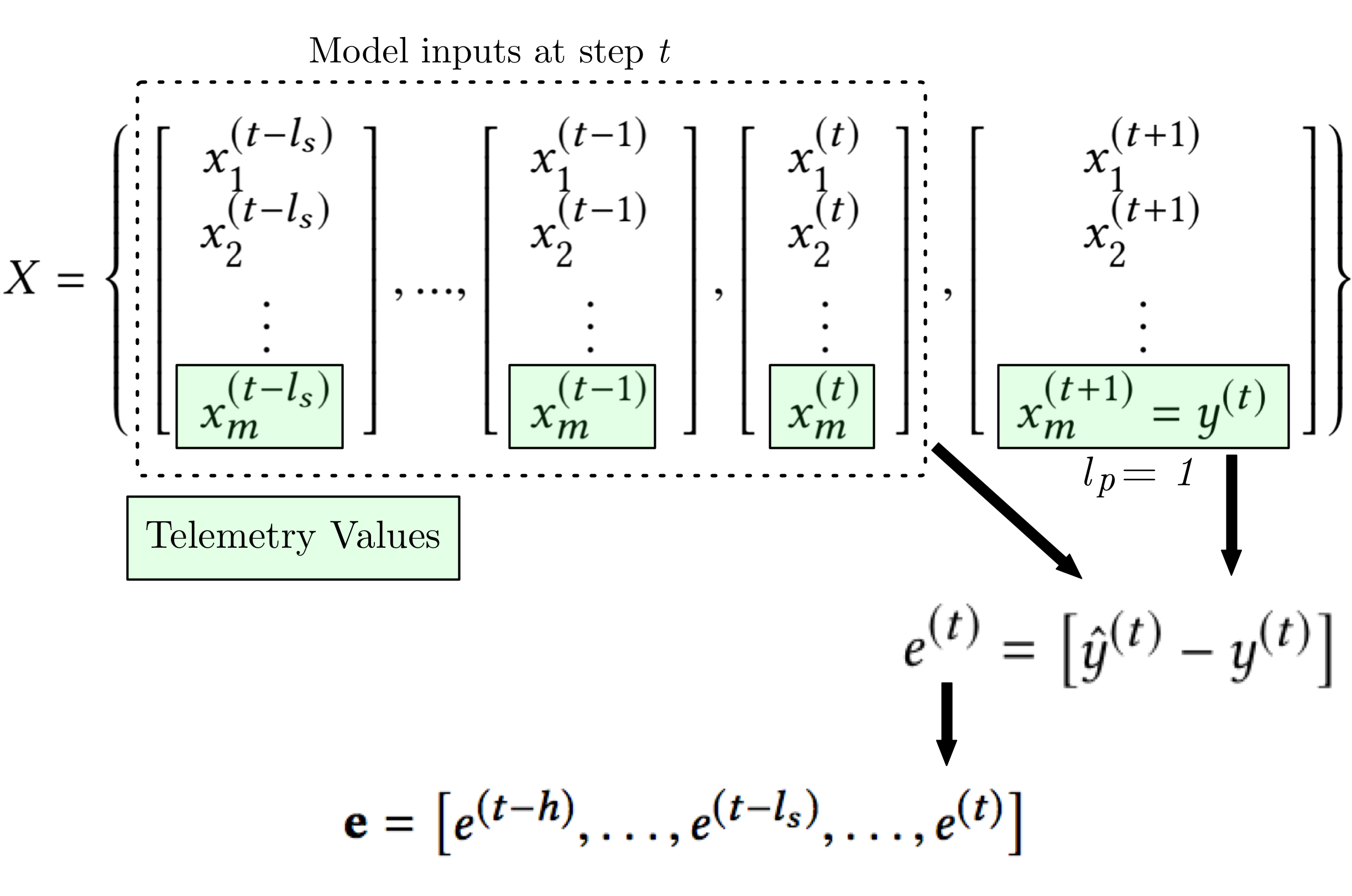
Figure 1. A visual representation of the input matrices used for prediction at each time step $t$. Current prediction errors are compared to past errors to determine if they are anomalous.

Predicting Values for a Channel. Consider a time series
$X=\{\textbf{x}^{(1)},\textbf{x}^{(2)},\ldots,\textbf{x}^{(n)}\}$ where each step $\textbf{x}^{(t)}\in R^{m}$ in the time series is an $m$-dimensional vector $\{x_{1}^{(t)},x_{2}^{(t)},\ldots,x_{m}^{(t)}\}$, whose elements correspond to input variables (Malhotra et al., 2015). For each point $\textbf{x}^{(t)}$, a sequence length $l_{s}$ determines the number of points to input into the model for prediction. A prediction length $l_{p}$ then determines the number of steps ahead to predict, where the number of dimensions $d$ being predicted is $1\leq d\leq m$. Since our aim is to predict telemetry values for a single channel we consider the situation where $d=1$. We also use $l_{p}=1$ to limit the number of predictions for each step $t$ and decrease processing time. As a result, a single scalar prediction $\hat{y}^{(t)}$ is generated for the actual telemetry value at each step $t$ (see Figure 1). In situations where either $l_{p}>1$ or $d>1$ or both, Gaussian parameters can be used to represent matrices of predicted values at a single step $t$ (Malhotra et al., 2015).

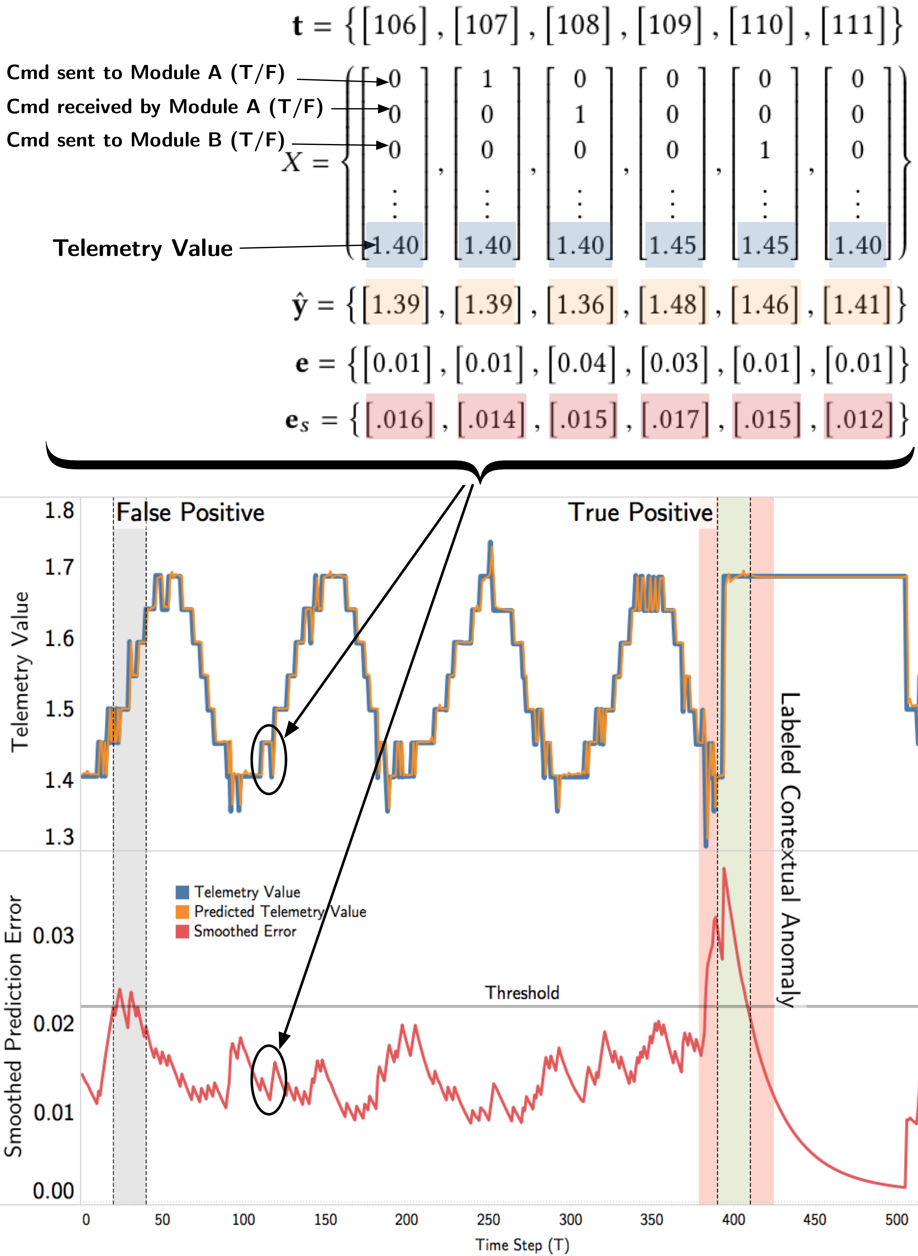
Figure 3. The encoding the of command information is demonstrated for a telemetry stream containing a contextual anomaly that is unlikely to be identified using limit- or distance-based approaches. Using the encoded command information and prior telemetry values for the channel, predictions are generated for the next time step with resulting errors. The one-step-ahead predictions and actual telemetry values are very close in this example as shown in top time series plot. An error threshold is set using the non-parametric thresholding approach detailed in Section 3.2, resulting in two predicted anomalous sequences – one false positive and one true positive lying within the labeled anomalous region. The false positive demonstrates the need for pruning described in Section 3.3, which would reclassify that sequence as nominal given that it is relatively close to values below the threshold (see Figure 2).

In our telemetry prediction scenario, the inputs $\textbf{x}^{(t)}$ into the LSTM consist of prior telemetry values for a given channel and encoded command information sent to the spacecraft. Specifically, the combination of the module to which a command was issued and whether a command was sent or received are one-hot encoded and slotted into each step $t$ (see Figure 3).

3.2. Dynamic Error Thresholds

Automated monitoring of thousands of telemetry channels whose expected values vary according to changing environmental factors and command sequences requires a fast, general, and unsupervised approach for determining if predicted values are anomalous. One common approach is to make Gaussian assumptions about the distributions of past smoothed errors as this allows for fast comparisons between new errors and compact representations of prior ones (Ahmad et al., 2017; Shipmon et al., 2017). However, this approach often becomes problematic when parametric assumptions are violated as we demonstrate in Section 4.3, and we offer an approach that efficiently identifies extreme values without making such assumptions. Distance-based methods are similar in this regard but they often involve high computational cost, such as those that call for comparisons of each point to a set of $k$ neighbors (Gao et al., 2012; Kriegel et al., 2009b). Also, these methods are more general and are concerned with anomalies that occur in the normal range of values. Only abnormally high or low smoothed prediction errors are of interest and error thresholding is, in a sense, a simplified version of the initial anomaly detection problem.

Errors and Smoothing. Once a predicted value $\hat{y}^{(t)}$ is generated for each step $t$, the prediction error is calculated as $e^{(t)}=|y^{(t)}-\hat{y}^{(t)}|$, where $y^{(t)}=x_{i}^{(t+1)}$ with $i$ corresponding to the dimension of the true telemetry value (see Figure 1). Each $e^{(t)}$ is appended to a one-dimensional vector of errors:

$$\textbf{e}=[e^{(t-h)},\ldots,e^{(t-l_{s})},\ldots,e^{(t-1)},e^{(t)}]$$

where $h$ is the number of historical error values used to evaluate current errors. The set of errors e are then smoothed to dampen spikes in errors that frequently occur with LSTM-based predictions – abrupt changes in values are often not perfectly predicted and result in sharp spikes in error values even when this behavior is normal (Shipmon et al., 2017). We use an exponentially-weighted average (EWMA) to generate the smoothed errors $\textbf{e}_{s}=[e_{s}^{(t-h)},\ldots,e_{s}^{(t-l_{s})},\ldots,e_{s}^{(t-1)},e_{s}^{(t)}]$ (Hunter et al., 1986). To evaluate whether values are nominal, we set a threshold for their smoothed prediction errors – values corresponding to smoothed errors above the threshold are classified as anomalies.

Threshold Calculation and Anomaly Scoring. At this stage, an appropriate anomaly threshold is sometimes learned with supervised methods that use labeled examples, however it is often the case that sufficient labeled data is not available and this holds true in our scenario (Chandola et al., 2009). We propose an unsupervised method that achieves high performance with low overhead and without the use of labeled data or statistical assumptions about errors. With a threshold $\epsilon$ selected from the set:

$$\boldsymbol{\epsilon}=\mu(\textbf{e}_{s})+\textbf{z}\sigma(\textbf{e}_{s})$$

Where $\epsilon$ is determined by:

$$\epsilon=argmax(\boldsymbol{\epsilon})=\frac{\Delta\mu(\textbf{e}_{s})/\mu(\textbf{e}_{s}))+(\Delta\sigma(\textbf{e}_{s})/\sigma(\textbf{e}_{s})}{|\textbf{e}_{a}|+|\textbf{E}_{seq}|^{2}}$$

Such that:
$\Delta\mu(\textbf{e}_{s})=\mu(\textbf{e}_{s})-\mu(\{e_{s}\in\textbf{e}_{s}|e_{s}<\epsilon\})$
$\Delta\sigma(\textbf{e}_{s})=\sigma(\textbf{e}_{s})-\sigma(\{e_{s}\in\textbf{e}_{s}|e_{s}<\epsilon\})$
$\textbf{e}_{a}=\{e_{s}\in\textbf{e}_{s}|e_{s}>\epsilon\}$
$\textbf{E}_{seq}=$ continuous sequences of $e_{a}\in\textbf{e}_{a}$

Values evaluated for $\epsilon$ are determined using $z\in\textbf{z}$ where $\mathbf{z}$ is an ordered set of positive values representing the number of standard deviations above $\mu(\textbf{e}_{s})$. Values for $\mathbf{z}$ depend on context, but we found a range of between two and ten to work well based on our experimental results. Values for $z$ less than two generally resulted in too many false positives. Once $argmax(\boldsymbol{\epsilon})$ is determined, each resulting anomalous sequence of smoothed errors $\textbf{e}_{seq}\in\textbf{E}_{seq}$ is given an anomaly score, $s$, indicating the severity of the anomaly:

$$s^{(i)}=\frac{max(\textbf{e}_{seq}^{(i)})-argmax(\boldsymbol{\epsilon})}{\mu(\textbf{e}_{s})+\sigma(\textbf{e}_{s})}$$

In simple terms, a threshold is found that, if all values above are removed, would cause the greatest percent decrease in the mean and standard deviation of the smoothed errors $\textbf{e}_{s}$. The function also penalizes for having larger numbers of anomalous values ($|\textbf{e}_{a}|$) and sequences ($|\textbf{E}_{seq}|$) to prevent overly greedy behavior. Then the highest smoothed error in each sequence of anomalous errors is given a normalized score based on its distance from the chosen threshold.

3.3. Mitigating False Positives

Pruning Anomalies. The precision of prediction-based anomaly detection approaches heavily depends on the amount of historical data ($h$) used to set thresholds and make judgments about current prediction errors. At large scales it becomes expensive to query and process historical data in real-time scenarios and a lack of history can lead to false positives that are only deemed anomalous because of the narrow context in which they are evaluated. Additionally, when extremely high volumes of data are being processed a low false positive rate can still overwhelm human reviewers charged with evaluating potentially anomalous events.

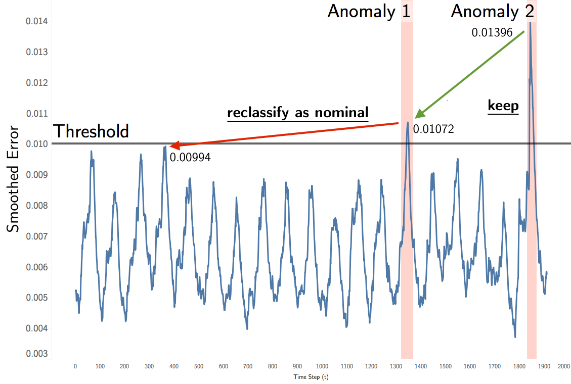
Figure 2. An example demonstrating the anomaly pruning process. In this scenario $\textbf{e}_{max}=[0.01396,0.01072,0.00994]$ and the minimum percent decrease $p=0.1$. The decrease from Anomaly 2 to Anomaly 1 $d^{(1)}=0.23>p$ and this sequence retains its classification as anomalous. From Anomaly 1 to the next highest smoothed error ($e_{s}=0.0099$) $d^{(2)}=.07<p$ so this sequence is re-classified as nominal.

To mitigate false positives and limit memory and compute cost, we introduce a pruning procedure in which a new set, $\textbf{e}_{max}$, is created containing $max(\textbf{e}_{seq})$ for all $\textbf{e}_{seq}$ sorted in descending order. We also add the maximum smoothed error that isn’t anomalous, $max(\{e_{s}\in\textbf{e}_{s}\in\textbf{E}_{seq}|e_{s}\ni\textbf{e}_{a}\})$, to the end of $\textbf{e}_{max}$. The sequence is then stepped through incrementally and the percent decrease $d^{(i)}=(e_{max}^{(i-1)}-e_{max}^{(i)})/e_{max}^{(i-1)}$ at each step $i$ is calculated where $i\in\{1,2,...,(|\textbf{E}_{seq}|+1)\}$. If at some step $i$ a minimum percentage decrease $p$ is exceeded by $d^{(i)}$, all $e_{max}^{(j)}\in\textbf{e}_{max}|\ j<i$ and their corresponding anomaly sequences remain anomalies. If the minimum decrease $p$ is not met by $d^{(i)}$ and for all subsequent errors $d^{(i)},d^{(i+1)},\ldots,d^{(i+|\textbf{E}_{seq}|+1)}$ those smoothed error sequences are reclassified as nominal. This pruning helps ensures anomalous sequences are not the result of regular noise within a stream, and it is enabled through the initial identification of sequences of anomalous values via thresholding. Limiting evaluation to only the maximum errors in a handful of potentially anomalous sequences is much more efficient than the multitude of value-to-value comparisons required without thresholding.

Learning from History. A second strategy for limiting false positives can be employed once a small amount of anomaly history or labeled data has been gathered. Based on the assumption that anomalies of similar magnitude $s$ generally are not frequently recurring within the same channel, we can set a minimum score, $s_{min}$, such that future anomalies are re-classified as nominal if $s<s_{min}$. A minimum score would only be applied to channels of data for which the system was generating anomalies above a certain rate and $s_{min}$ is individually set for all such channels. Prior anomaly scores for a channel can be used to set an appropriate $s_{min}$ depending on the desired balance between precision and recall.

Additionally, if the anomaly detection system has a mechanism by which users can provide labels for anomalies, these labels can also be used to set $s_{min}$ for a given stream. For example, if a stream or channel has several confirmed false positive anomalies, $s_{min}$ can be set near the upper bound of these false positive anomaly scores. Both of these approaches have played an important role in improving the precision of early implementations of the system by helping account for normal spacecraft behaviors that are infrequent but occur at regular intervals.

4. Experiments

For many spacecraft including SMAP and MSL, current anomaly detection systems are difficult to assess. The precision and recall of alarms aren’t captured and telemetry assessments are often performed manually. Fortunately, indications of telemetry anomalies can be found within previously mentioned ISA reports. A subset of all of the incidents and anomalies detailed in ISAs manifest in specific telemetry channels, and by mining the ISA reports for SMAP and MSL we were able to collect a set of telemetry anomalies corresponding to actual spacecraft issues involving various subsystems and channel types.

Table 1. Experimental Data Information

	SMAP	MSL	Total
Total anomaly sequences	69	36	105
Point anomalies (% tot.)	43 (62%)	19 (53%)	62 (59%)
Contextual anomalies (% tot.)	26 (38%)	17 (47%)	43 (41%)
Unique telemetry channels	55	27	82
Unique ISAs	28	19	47
Telemetry values evaluated	429,735	66,709	496,444

All telemetry channels discussed in an individual ISA were reviewed to ensure that the anomaly was evident in the associated telemetry data, and specific anomalous time ranges were manually labeled for each channel. If multiple anomalous sequences and channels closely resembled each other, only one was kept for the experiment in order to create a diverse and balanced set.

We classify anomalies into two categories, point and contextual, to distinguish between anomalies that would likely be identified by properly-set alarms or distance-based methods that ignore temporal information (point anomalies) and those that require more complex methodologies such as LSTMs or Hierarchical Temporal Memory (HTM) approaches to detect (contextual anomalies)(Ahmad et al., 2017). This characterization is adapted from the three categories previously mentioned – point, contextual, and collective (Chandola et al., 2009). Since contextual and collective anomalies both require temporal context and are harder to detect, they have both been combined into the contextual category presented in the next section.

In addition to evaluating the performance of the methodologies in Section 3, we also compare the post-prediction performance of our error thresholding method to a parametric unsupervised approach used in the top-performing algorithm for the recent Numenta Anomaly Benchmark (Ahmad et al., 2017; Lavin and Ahmad, 2015).

No comparisons are made between the LSTM-based approach and other predictive models as leaps forward in the underlying prediction performance will more likely come from providing increasingly refined command-based features to the model. Given the rise in prediction-based anomaly detection methods and related research (Malhotra et al., 2016, 2015), we place increased emphasis on post-prediction error evaluation methods that have received comparatively less focus yet demonstrate significant impact on our results.

4.1. Setup

For each unique stream of data containing one or more anomalous sequences with the primary anomaly occurring at time $t_{a}$, we evaluate all telemetry values in a surrounding timeframe from $t_{s}=t_{a}-3d$ to $t_{f}=t_{a}+2d$ where $d$ is days. A model is trained for each unique stream using values and command data from $t_{s_{train}}=t_{s}-2d$ to $t_{f_{train}}=t_{s}$. Additional days were included if sufficient data was not available in these timeframes. This 5-day span around anomalies was selected to balance two objectives: deeper insight into precision and reasonable computational cost. Predicted anomalous regions are also slightly expanded to facilitate the combining of anomalous regions in close proximity – regions that overlap or touch after expansion are combined into a single region to account for situations where multiple anomalous regions represent a single event.

Each labeled anomalous sequence $x_{a}\in\textbf{x}_{a}$ of telemetry values is evaluated against the final set of predicted anomalous sequences identified by the system according to the following rules:

1. A true positive is recorded if:

   $$|e_{a}^{(t)}\in e_{seq}\in\textbf{e}_{seq}:x_{i}^{(t)}\in x_{a}|>0$$

   for any $x_{a}\in\textbf{x}_{a}$. In other words, a true positive results if any portion of a predicted sequence of anomalies falls within any true labeled sequence. Only one true positive is recorded even if portions of multiple predicted sequences fall within a labeled sequence.

2. If no predicted sequences overlap with a positively labeled sequence, a false negative is recorded for the labeled sequence.

3. For all predicted sequences that do not overlap a labeled anomalous region, a false positive is recorded.

For simplicity, we do not make scoring adjustments based on how early an anomaly was detected or the distance between false positives and labeled regions (Lavin and Ahmad, 2015).

Batch processing. Telemetry values are aggregated into one minute windows and evaluated in batches of 70 minutes mimicking the downlink schedule for SMAP and our current system implementation. Each 70 minute batch of values is evaluated using $h=2100$, where $h$ is the number of prior values used to calculate an error threshold and evaluate the current batch. The system is also well-suited to process values in a real-time, streaming fashion when applicable.

4.2. Model Parameters and Evaluation

The same architecture and parameters are used for all models in the experiment:

Model Parameters
hidden layers	2
units in hidden layers	80
sequence length ($l_{s}$)	250
training iterations	35
dropout	0.3
batch size	64
optimizer	Adam
input dimensions	25 (SMAP), 55 (MSL)

Each model is shallow with only two hidden layers and 80 units in each layer. We found this architecture provided enough capacity to predict individual channels well, and adding additional capacity provided little to no prediction benefits while increasing model sizes and training times. All channels do not necessarily require this amount of capacity and future improvements could include automated selection of appropriate model capacity based on channel complexity. Similarly, a sequence length $l_{s}=250$ provided a balance between performance and training times. The difference in input dimensions for SMAP and MSL results from the missions each having different sets of command modules. Early stopping was used to prevent overfitting during model training, and not all models were trained for the full 35 iterations.

Once predictions were generated, anomaly thresholds for smoothed errors were calculated using the method detailed in Section 3.2 with $\textbf{z}=\{2.5,3.0,3.5,...,10.0\}$ and the minimum percent difference between subsequent anomalies $p=0.13$. The $p$ parameter is an important lever for controlling precision and recall, and an appropriate value can be inferred when labels are available. In our setting, reasonable results were achieved with $0.05<p<0.20$ (see Figure 4).

Comparison with Parametric Thresholding. Using the raw LSTM prediction errors, we also generate anomalies with the parametric error evaluation approach used in coordination with the most accurate model from the Numenta Anomaly Benchmark (Lavin and Ahmad, 2015). This approach processes raw errors incrementally – at each step $t$ a window $W$ of historical errors is modeled as a normal distribution, and the mean $\mu_{W}$ and variance $\sigma_{W}^{2}$ are updated at each step $t$. We set $W$’s length $l_{w}=h=2100$ and use the same set of prediction errors for both approaches. A short-term average $\mu_{s}$ of length $l_{short}$ of prediction errors is then calculated and has a similar smoothing effect as the EWMA smoothing in Section 3.2. The likelihood of an anomaly $L$ is then defined using the tail probability $Q$:

$$L=1-Q\left(\frac{\mu_{s}-\mu_{W}}{\sigma_{W}^{2}}\right)$$

If $L\geq 1-\epsilon_{norm}$ values are classified as anomalous. In the next section, results generated using $l_{short}=10$ and $\epsilon_{norm}=\{0.01,0.0001\}$ are compared to the approach in Section 3.2. The effects of pruning (detailed in Section 3.3) on this approach are also tested.

4.3. Results and Discussion

Table 2. Results for each spacecraft using LSTM predictions and various approaches to error thresholding.

Thresholding Approach	Precision	Recall	$F_{0.5}$ score
Non-Parametric w/ Pruning ($p=0.13$)
MSL	92.6%	69.4%	0.69
SMAP	85.5%	85.5%	0.71
Total	87.5%	80.0%	0.71
Non-Parametric w/out Pruning ($p=0$)
MSL	75.8%	69.4%	0.61
SMAP	43.0%	92.8%	0.44
Total	48.9%	84.8%	0.47
Gaussian Tail ($\epsilon_{norm}=0.0001$)
MSL	84.2%	44.4%	0.54
SMAP	88.5%	78.3%	0.71
Total	87.5%	66.7%	0.66
Gaussian Tail ($\epsilon_{norm}=0.01$)
MSL	61.3%	52.8%	0.48
SMAP	82.4%	81.2%	0.68
Total	75.8%	71.4%	0.62
Gaussian Tail w/ Pruning ($\epsilon_{norm}=0.01,p=0.13$)
MSL	88.2%	41.7%	0.54
SMAP	92.7%	73.9%	0.71
Total	91.7%	62.9%	0.66

As shown in Table 2, the best results in terms of $F_{0.5}$ score are achieved using the LSTM-based predictions combined with the non-parametric thresholding approach with pruning. In terms of prediction, The LSTM models achieved an average normalized absolute error of 5.9% predicting telemetry values one time step ahead.

Table 3. Telemetry Prediction Errors

Average LSTM Prediction Error
move! MSL	6.8%
move !SMAP	5.5%
move!Total	5.9%

Parameters were tuned to balance precision and recall for experimentation, however in the current implementation precision is weighted more heavily when tuning parameters because the precision results shown are overly optimistic compared to the actual implementation of the system. There is an implicit assumption in the experiment that anomalies occur once every five days, where five days is the total number of days processed for each stream containing an anomaly. The experiment also does not include processing for all streams not exhibiting anomalous behavior for a given time window, which would further increase the number of false positives. This decreased precision in the implemented system is offset by setting minimum anomaly scores via the methods outlined at the end of Section 3.3.

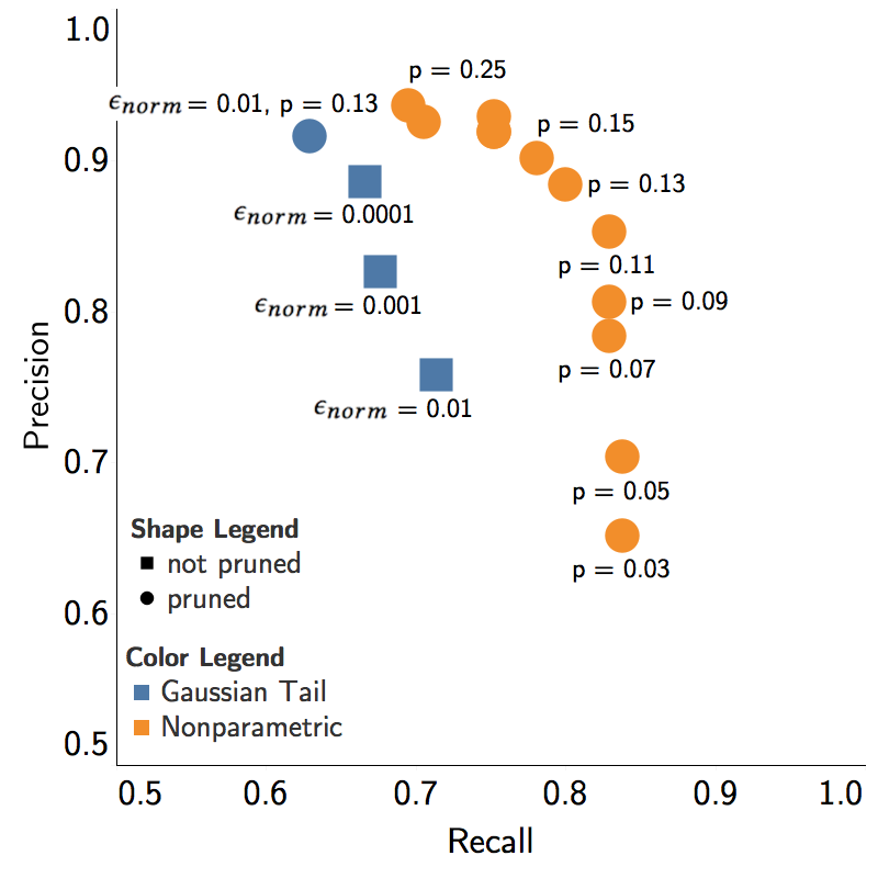
Figure 4. Plot showing comparison of overall precision and recall results for parametric approach and approach presented in this paper (labeled ’Nonparametric’) with various parameter settings.

Thresholding Comparisons. Results for the non-parametric approach without pruning are presented to demonstrate pruning’s importance in mitigating false positives. The pruning process is roughly analogous to the pruning of decision trees in the sense that it helps pare down a greedy approach designed to overfit in order to improve performance. In this instance, pruning only decreases overall recall by 4.8 percentage points (84.8% to 80.0%) while increasing overall precision by 38.6 percentage points (48.9% to 87.5%). The 84.8% recall achieved without pruning is an approximation of the upper bound for recall given the predictions generated by the LSTM models. If predictions are poor and resulting smoothed errors do not contain a signal then thresholding methods will be ineffective.

The Gaussian tail approach results in lower levels of precision and recall using various parameter settings. Pruning greatly improves precision but at a high recall cost, resulting in an $F_{0.5}$ score that is still well below the score achieved by the non-parametric approach with pruning. One factor that contributes to lower performance for this method is the violation of Gaussian assumptions in the smoothed errors. Using D’Agostino and Pearson’s normality test (D’AGOSTINO and Pearson, 1973), we reject the null hypothesis of normality for all sets of smoothed errors using a threshold of $\alpha=0.005$. The error information lost when using Gaussian parameters results in suboptimal thresholds that negatively affect precision and recall and cannot be corrected by pruning (see Figure 4 and Table 2).

Performance for Different Anomaly Types. The high proportion of contextual anomalies (41%) provides further justification for the use of LSTMs and prediction-based methods over methods that ignore temporal information. Only a small subset of the contextual anomalies – those where anomalous telemetry values happen to fall in low-density regions – could theoretically be detected using limit-based or density-based approaches. Optimistically, this establishes a maximum possible recall near the best result presented here and obviates extensive comparisons with these approaches. Not surprisingly, recall was lower for contextual anomalies but the LSTM-based approach was able to identify a majority of these.

Table 4. Recall for different anomaly types using LSTM predictions with non-parametric thresholding and pruning.

	Recall - point	Recall - contextual
MSL	78.9%	58.8%
SMAP	95.3%	76.0%
Total	90.3%	69.0%

Performance for Different Spacecraft. SMAP and MSL are very different missions representing varying degrees of difficulty when it comes to anomaly detection. Compared to MSL, operations for the SMAP spacecraft are routine and resulting telemetry can be more easily predicted with less training and less data. MSL performs a much wider variety of behaviors with varying regularity, some of which resulted during rover activities that were not present in the limited training data. This explains the lower precision and recall performance for MSL ISAs and is also apparent in the difference between the average LSTM prediction errors - average error in predicting telemetry for SMAP was 5.5% versus 6.8% for MSL (see Table 3).

5. Deployment

The methods presented in this paper have been implemented into a system that is currently being piloted by SMAP operations engineers. Over 700 channels are being monitored in near real-time as data is downlinked from the spacecraft and models are trained offline every three days with early stopping. We have successfully identified several confirmed anomalies since the initial deployment in October 2017. However, one major obstacle to becoming a central component of the telemetry review process is the current rate of false positives. High demands are placed on operations engineers and they are hesitant to alter effective procedures. Adopting new technologies and systems means increased risk of wasting valuable time and attention. Investigation of even a couple false positives can deter users and therefore achieving high precision with over a million telemetry values being processed per day is essential for adoption.

Future Work. The pilot deployment and experimental results are key milestones in establishing that a large-scale, automated telemetry monitoring system is feasible. Future work will be focused around improving telemetry predictions primarily through improved feature engineering.

Spacecraft command information is only one-hot encoded at the module level in the current implementation, and no information about the nature of the command itself is passed to the models. Much more granular information around command activity and other sources of information like event records may be necessary to accurately predict telemetry data for missions without routine operations. For these missions, training data from periods with similar activities to those planned must be automatically identified and selected rather than simply training on recent activity. Accurate predictions are critical to this approach and will allow the system to be extended to missions like MSL while also addressing the need for improved precision. The two aforementioned improvements represent key areas of future work that will be generally beneficial for monitoring dynamic and complex spacecraft. We also plan to continue to refine our approaches to mitigating false positives described in Section 3.3 and improve interfaces facilitating the review, investigation, and expert labeling of anomalies found by the system.

Lastly, another key aspect of our problem that has not been addressed are the interactions and dependencies inherent in the telemetry channels. This has been partially addressed through a visual interface, but a more mathematical and automated view into the correlations between channel anomalies would provide important insight into complex system behaviors and anomalies.

6. Conclusion

This paper presents and defines an important and growing challenge within spacecraft operations that stands to greatly benefit from modern anomaly detection approaches. We demonstrate the viability of LSTMs for predicting spacecraft telemetry while addressing key challenges involving interpretability, scale, precision, and complexity that are inherent in many anomaly detection scenarios. We also propose a novel dynamic thresholding approach that does not rely on scarce labels or false parametric assumptions. Key areas for improvement and further evaluation have also been identified as we look to expand capabilities and implement systems for a variety of spacecraft. Finally, we make public a large real-world, expert-labeled set of anomalous spacecraft telemetry data and offer open-source implementations of the methodologies presented in this paper.

- (1)
- nas (2018) 2018. Getting Ready for NISAR-and for Managing Big Data using the Commercial Cloud — Earthdata. https://earthdata.nasa.gov/getting-ready-for-nisar
- Ahmad et al. (2017) Subutai Ahmad, Alexander Lavin, Scott Purdy, and Zuha Agha. 2017. Unsupervised real-time anomaly detection for streaming data. Neurocomputing 262 (2017), 134–147.
- Bay and Schwabacher (2003) Stephen D. Bay and Mark Schwabacher. 2003. Mining Distance-based Outliers in Near Linear Time with Randomization and a Simple Pruning Rule. In Proceedings of the Ninth ACM SIGKDD International Conference on Knowledge Discovery and Data Mining (KDD ’03). ACM, New York, NY, USA, 29–38. https://doi.org/10.1145/956750.956758
- Bernard et al. (1999) D. Bernard, R. Doyle, E. Riedel, N. Rouquette, J. Wyatt, M. Lowry, and P. Nayak. 1999. Autonomy and software technology on NASA’s Deep Space One. IEEE Intelligent Systems 14, 3 (may 1999), 10–15. https://doi.org/10.1109/5254.769876
- Bontemps et al. (2017) Loic Bontemps, Van Loi Cao, James McDermott, and Nhien-An Le-Khac. 2017. Collective Anomaly Detection based on Long Short Term Memory Recurrent Neural Network. arXiv:arXiv:1703.09752
- Breunig et al. (2000) Markus Breunig, Hans-Peter Kriegel, Raymond T. Ng, and Jörg Sander. 2000. LOF: Identifying Density-Based Local Outliers. In PROCEEDINGS OF THE 2000 ACM SIGMOD INTERNATIONAL CONFERENCE ON MANAGEMENT OF DATA. ACM, 93–104.
- C. et al. (1992) Chang C., Nallo W., Rastogi R., Beugless D., Mickey F., and Shoop A. 1992. Satellite diagnostic system: An expert system for intelsat satellite operations. In In Proceedings of the IVth European Aerospace Conference (EAC). 321–327.
- Caruana et al. (2001) Rich Caruana, Steve Lawrence, and C Lee Giles. 2001. Overfitting in neural nets: Backpropagation, conjugate gradient, and early stopping. In Advances in neural information processing systems. 402–408.
- Chandola et al. (2009) Varun Chandola, Arindam Banerjee, and Vipin Kumar. 2009. Anomaly Detection: A Survey. ACM Comput. Surv. 41, 3, Article 15 (jul 2009), 58 pages. https://doi.org/10.1145/1541880.1541882
- Chauhan and Vig (2015) Sucheta Chauhan and Lovekesh Vig. 2015. Anomaly detection in ECG time signals via deep long short-term memory networks. In 2015 IEEE International Conference on Data Science and Advanced Analytics (DSAA). IEEE. https://doi.org/10.1109/dsaa.2015.7344872
- Ciceri and Marradi (1994) F. Ciceri and L. Marradi. 1994. Event diagnosis and recovery in real-time on-board autonomous mission control. In Ada in Europe. Springer Berlin Heidelberg, 288–301. https://doi.org/10.1007/3-540-58822-1_107
- D’AGOSTINO and Pearson (1973) RALPH D’AGOSTINO and Egon S Pearson. 1973. Tests for departure from normality. Empirical results for the distributions of b 2 and√ b. Biometrika 60, 3 (1973), 613–622.
- Fuertes et al. (2016) Sylvain Fuertes, Gilles Picart, Jean-Yves Tourneret, Lotfi Chaari, André Ferrari, and Cédric Richard. 2016. Improving Spacecraft Health Monitoring with Automatic Anomaly Detection Techniques. In 14th International Conference on Space Operations (SpaceOps 2016). pp–1.
- Fujimaki et al. (2005) Ryohei Fujimaki, Takehisa Yairi, and Kazuo Machida. 2005. An Approach to Spacecraft Anomaly Detection Problem Using Kernel Feature Space. In Proceedings of the Eleventh ACM SIGKDD International Conference on Knowledge Discovery in Data Mining (KDD ’05). ACM, New York, NY, USA, 401–410. https://doi.org/10.1145/1081870.1081917
- Gao et al. (2012) Yu Gao, Tianshe Yang, Minqiang Xu, and Nan Xing. 2012. An Unsupervised Anomaly Detection Approach for Spacecraft Based on Normal Behavior Clustering. In 2012 Fifth International Conference on Intelligent Computation Technology and Automation. IEEE. https://doi.org/10.1109/icicta.2012.126
- Goldstein and Uchida (2016) Markus Goldstein and Seiichi Uchida. 2016. A Comparative Evaluation of Unsupervised Anomaly Detection Algorithms for Multivariate Data. PLOS ONE 11, 4 (apr 2016), e0152173. https://doi.org/10.1371/journal.pone.0152173
- Goodfellow et al. (2016) Ian Goodfellow, Yoshua Bengio, Aaron Courville, and Yoshua Bengio. 2016. Deep learning. Vol. 1. MIT press Cambridge.
- Graves (2012) Alex Graves. 2012. Supervised Sequence Labelling with Recurrent Neural Networks. Springer Berlin Heidelberg. https://doi.org/10.1007/978-3-642-24797-2
- Graves et al. (2013) Alex Graves, Abdel rahman Mohamed, and Geoffrey Hinton. 2013. Speech Recognition with Deep Recurrent Neural Networks. arXiv:arXiv:1303.5778
- Hand et al. (2017) KP Hand, AE Murray, JB Garvin, WB Brinckerhoff, BC Christner, KS Edgett, BL Ehlmann, C German, AG Hayes, TM Hoehler, et al. 2017. Report of the Europa Lander Science Definition Team. Posted February (2017).
- Hochreiter and Schmidhuber (1997) Sepp Hochreiter and Jürgen Schmidhuber. 1997. Long Short-Term Memory. Neural Comput. 9, 8 (nov 1997), 1735–1780. https://doi.org/10.1162/neco.1997.9.8.1735
- Hunter et al. (1986) J Stuart Hunter et al. 1986. The exponentially weighted moving average. J. Quality Technol. 18, 4 (1986), 203–210.
- Iverson (2008) David Iverson. 2008. Data Mining Applications for Space Mission Operations System Health Monitoring. In SpaceOps 2008 Conference. American Institute of Aeronautics and Astronautics. https://doi.org/10.2514/6.2008-3212
- Iverson (2004) David L. Iverson. 2004. Inductive system health monitoring. In In Proceedings of The 2004 International Conference on Artificial Intelligence (IC-AI04), Las Vegas. CSREA Press.
- Kriegel et al. (2009a) Hans-Peter Kriegel, Peer Kröger, Erich Schubert, and Arthur Zimek. 2009a. LoOP: Local Outlier Probabilities. In Proceedings of the 18th ACM Conference on Information and Knowledge Management (CIKM ’09). ACM, New York, NY, USA, 1649–1652. https://doi.org/10.1145/1645953.1646195
- Kriegel et al. (2009b) Hans-Peter Kriegel, Peer Kröger, Erich Schubert, and Arthur Zimek. 2009b. LoOP: local outlier probabilities. In Proceedings of the 18th ACM conference on Information and knowledge management. ACM, 1649–1652.
- Lavin and Ahmad (2015) Alexander Lavin and Subutai Ahmad. 2015. Evaluating Real-Time Anomaly Detection Algorithms–The Numenta Anomaly Benchmark. In Machine Learning and Applications (ICMLA), 2015 IEEE 14th International Conference on. IEEE, 38–44.
- Li et al. (2016) Ke Li, Yalei Wu, Shimin Song, Yi sun, Jun Wang, and Yang Li. 2016. A novel method for spacecraft electrical fault detection based on FCM clustering and WPSVM classification with PCA feature extraction. Proceedings of the Institution of Mechanical Engineers, Part G: Journal of Aerospace Engineering 231, 1 (aug 2016), 98–108. https://doi.org/10.1177/0954410016638874
- Li et al. (2010) Quan Li, XingShe Zhou, Peng Lin, and Shaomin Li. 2010. Anomaly detection and fault Diagnosis technology of spacecraft based on telemetry-mining. In 2010 3rd International Symposium on Systems and Control in Aeronautics and Astronautics. IEEE. https://doi.org/10.1109/isscaa.2010.5633180
- Malhotra et al. (2015) Pankaj Malhotra, Vig Lovekesh, Gautam Shroff, and Puneet Argarwal. 2015. Long Short Term Memory Networks for Anomaly Detection in Time Series. In In Proceedings of the European Symposium on Artificial Neural Networks (ESANN), Computational Intelligence and Machine Learning.
- Malhotra et al. (2016) Pankaj Malhotra, Anusha Ramakrishnan, Gaurangi Anand, Lovekesh Vig, Puneet Agarwal, and Gautam Shroff. 2016. LSTM-based Encoder-Decoder for Multi-sensor Anomaly Detection. CoRR abs/1607.00148 (2016).
- Martínez-Heras and Donati (2014) Jose Martínez-Heras and Alessandro Donati. 2014. Enhanced Telemetry Monitoring with Novelty Detection. 35 (12 2014), 37–46.
- Nanduri and Sherry (2016) Anvardh Nanduri and Lance Sherry. 2016. Anomaly detection in aircraft data using Recurrent Neural Networks (RNN). 2016 Integrated Communications Navigation and Surveillance (ICNS) (2016), 5C2–1–5C2–8.
- Nishigori and Limited (2001) Naomi Nishigori and Fujitsu Limited. 2001. Fully Automatic and Operator-less Anomaly Detecting Ground Support System For Mars Probe ”NOZOMI”. In In Proceedings of the 6th International Symposium on Artificial Intelligence and Robotics and Automation in Space (i-SAIRAS).
- Ogunmolu et al. (2016) Olalekan Ogunmolu, Xuejun Gu, Steve Jiang, and Nicholas Gans. 2016. Nonlinear Systems Identification Using Deep Dynamic Neural Networks. arXiv:arXiv:1610.01439
- Rolincikm et al. (1992) M. Rolincikm, Lauriente M., Koons H., and D. Gorney. 1992. An expert system for diagnosing environmentally induced spacecraft anomalies. Technical Report. NASA. Lyndon B. Johnson Space Center, Fifth Annual Workshop on Space Operations Applications and Research (SOAR 1991).
- Sak et al. (2014) Haşim Sak, Andrew Senior, and Françoise Beaufays. 2014. Long Short-Term Memory Based Recurrent Neural Network Architectures for Large Vocabulary Speech Recognition. arXiv:arXiv:1402.1128
- Schmidhuber (2015) Jürgen Schmidhuber. 2015. Deep learning in neural networks: An overview. Neural Networks 61 (jan 2015), 85–117. https://doi.org/10.1016/j.neunet.2014.09.003
- Schölkopf et al. (1998) Bernhard Schölkopf, Alexander Smola, and Klaus-Robert Müller. 1998. Nonlinear Component Analysis As a Kernel Eigenvalue Problem. Neural Comput. 10, 5 (July 1998), 1299–1319. https://doi.org/10.1162/089976698300017467
- Sherwood et al. ([n. d.]) R. Sherwood, A. Schlutsmeyer, M. Sue, and E.J. Wyatt. [n. d.]. Lessons from implementation of beacon spacecraft operations on Deep Space One. In 2000 IEEE Aerospace Conference. Proceedings (Cat. No.00TH8484). IEEE. https://doi.org/10.1109/aero.2000.878245
- Shipmon et al. (2017) Dominique T. Shipmon, Jason M. Gurevitch, Paolo M. Piselli, and Stephen T. Edwards. 2017. Time Series Anomaly Detection; Detection of anomalous drops with limited features and sparse examples in noisy highly periodic data. arXiv:arXiv:1708.03665
- Sutskever et al. (2014) Ilya Sutskever, Oriol Vinyals, and Quoc V. Le. 2014. Sequence to Sequence Learning with Neural Networks. arXiv:arXiv:1409.3215
- Tallo et al. (1992) Donald P. Tallo, John Durkin, and Edward J. Petrik. 1992. Intelligent fault isolation and diagnosis for communication satellite systems. Telematics and Informatics 9, 3-4 (jun 1992), 173–190. https://doi.org/10.1016/s0736-5853(05)80035-8
- Taylor et al. (2016) Adrian Taylor, Sylvain Leblanc, and Nathalie Japkowicz. 2016. Anomaly Detection in Automobile Control Network Data with Long Short-Term Memory Networks. In 2016 IEEE International Conference on Data Science and Advanced Analytics (DSAA). IEEE. https://doi.org/10.1109/dsaa.2016.20
- Yairi ([n. d.]) Yoshinobu Kawahara Takehisa Yairi. [n. d.]. Telemetry-mining: A Machine Learning Approach to Anomaly Detection and Fault Diagnosis for Space Systems. In 2nd IEEE International Conference on Space Mission Challenges for Information Technology. IEEE. https://doi.org/10.1109/smc-it.2006.79
- Young et al. (2017) Tom Young, Devamanyu Hazarika, Soujanya Poria, and Erik Cambria. 2017. Recent Trends in Deep Learning Based Natural Language Processing. arXiv:arXiv:1708.02709
- Zhou et al. (2016) Peng Zhou, Zhenyu Qi, Suncong Zheng, Jiaming Xu, Hongyun Bao, and Bo Xu. 2016. Text Classification Improved by Integrating Bidirectional LSTM with Two-dimensional Max Pooling. arXiv:arXiv:1611.06639