On gravity’s role in the genesis of rest masses of classical fields

Abstract

It is shown that in the Einstein–conformally coupled Higgs–Maxwell system with Friedman–Robertson–Walker symmetries the energy density of the Higgs field has stable local minimum only if the mean curvature of the $t={\rm const}$ hypersurfaces is less than a finite critical value $\chi_{c}$, while for greater mean curvature the energy density is not bounded from below. Therefore, there are extreme gravitational situations in which even quasi-locally defined instantaneous vacuum states of the Higgs sector cannot exist, and hence one cannot at all define the rest mass of all the classical fields. On hypersurfaces with mean curvature less than $\chi_{c}$ the energy density has the ‘wine bottle’ (rather than the familiar ‘Mexican hat’) shape, and the gauge field can get rest mass via the Brout–Englert–Higgs mechanism. The spacelike hypersurface with the critical mean curvature represents the moment of ‘genesis’ of rest masses.

1 Introduction

In the conformal cyclic cosmological (or CCC) model of Penrose [1] all the particles and fields must be massless on a neighbourhood of the crossover hypersurfaces. (Such a hypersurface, as a regular spacelike hypersurface in the conformal spacetime, is the interface between two successive aeons, and represents the future conformal boundary of the previous and the big bang singularity of the subsequent aeon.) Thus, according to this model, the particles and fields had to loose their rest mass in the very late stage of the previous aeon, and got rest mass only after the Big Bang of our Universe in some mechanism. In particular, the particles and fields had to be massless in a neighbourhood of the Big Bang. Thus, in particle physics compatible with the CCC model, the rest masses should be expected to appear/disappear in some dynamical process.

The aim of the present paper is to clarify whether or not the rest mass of classical fields can appear/disappear in a dynamical process via the Brout–Englert–Higgs mechanism in a classical field theoretical model which mimics all the characteristic feature of the Einstein–Standard Model system.

1.1 The rest mass of relativistic classical fields

In the usual formulation of classical mechanics rest mass is an a priori given attribute of particles, which can be determined from their small oscillations in a potential field around the stable equilibrium state (see e.g. [2]). Hence, in a more positivist approach to mechanics, the notion of rest mass can be introduced via the study of small oscillations.

In the relativistic theory of classical fields the definition of the rest mass of the matter fields is based just on this idea. To illustrate this, let us consider a single real scalar field $\phi$ on the spacetime whose dynamics is governed by the Lagrangian ${\cal L}=\frac{1}{2}g^{ab}(\nabla_{a}\phi)(\nabla_{b}\phi)-U(\phi)$, where the potential $U$ may depend on further fields, say $\Phi$, and it is a local, algebraic expression of its variables. This yields the field equation $\nabla_{a}\nabla^{a}\phi+(\partial U/\partial\phi)=0$. Following the mechanical analogy, if the scalar field is constant on the spacetime manifold $M$, say $\phi_{0}$, then, by $\nabla_{a}\phi_{0}=0$, this may be considered as a ground or vacuum state (being analogous to the equilibrium configuration of the mechanical systems above). It solves the field equation precisely when $0=(\partial U/\partial\phi)_{0}=-(\partial{\cal L}/\partial\phi)_{0}$, where the subscript $0$ means ‘evaluated at $\phi_{0}$’. Thus, the ground states that solve the field equation are critical points of the potential. Hence, if we write $U(\phi)=U(\phi_{0})+(\partial U/\partial\phi)_{0}(\phi-\phi_{0})+\frac{1}{2}(\partial^{2}U/\partial\phi^{2})_{0}(\phi-\phi_{0})^{2}+...$, then the field equation yields

$$\nabla_{a}\nabla^{a}\bigl{(}\phi-\phi_{0}\bigr{)}=-\Bigl{(}\frac{\partial^{2}U}{\partial\phi^{2}}\Bigr{)}_{0}\bigl{(}\phi-\phi_{0}\bigr{)}+{\cal O}((\phi-\phi_{0})^{2}).$$ (1.1)

Let $p$ be any point of $M$ and $x^{\underline{a}\,}$ the Gaussian normal (or local, approximate Cartesian) coordinate system on an open neighbourhood $W$ of $p$, which is based on an orthonormal vector basis $\{E^{a}_{\underline{a}\,}\}$ and the origin at $p$ (see e.g. [3]). Let $k^{a}$ be a vector at $p$ with components $k^{\underline{a}\,}$ in the basis $\{E^{a}_{\underline{a}\,}\}$. Then (1.1) admits (local, approximate) solutions describing small linear oscillations on $W$ around $\phi_{0}$ with wave vector $k^{a}$, viz. $\phi_{k}(x^{\underline{a}\,})=\phi_{0}+A\cos(k_{\underline{a}\,}x^{\underline{a}\,})+B\sin(k_{\underline{a}\,}x^{\underline{a}\,})$ for $A,B\in\mathbb{R}$, precisely when

$$g_{ab}k^{a}k^{b}=\Bigl{(}\frac{\partial^{2}U}{\partial\phi^{2}}\Bigr{)}_{0}(p).$$ (1.2)

(Note that $(\partial^{2}U/\partial\phi^{2})_{0}$ may still depend on the spacetime point $p$ via the other fields, say $\Phi$. Also, in this linear, approximate solution we neglect the back reaction of the scalar field to the spacetime geometry, i.e. this solution is considered to be only a ‘test field’ to ‘scan’ some of the local properties of the physical system.)

By (1.2) the wave vector $k^{a}$ is spacelike, null or timelike precisely when the critical point $\phi_{0}$ of the potential is a maximum, an inflexion or a minimum point, respectively. Hence, the hypersurfaces in $W$ on which the solution $\phi_{k}(x^{\underline{a}\,})$ has constant phase, $k_{\underline{a}\,}x^{\underline{a}\,}={\rm const}$, are, respectively, timelike, null or spacelike. Thus it is only the case of non-spacelike wave vectors in which any observer sees $\phi_{k}(x^{\underline{a}\,})$ to be oscillating around $\phi_{0}$. For a spacelike wave vector there is a family of local Lorentz frames from which the solution $\phi_{k}(x^{\underline{a}\,})$ appears to describe standing waves rather than oscillations around $\phi_{0}$. The Lorentz invariant measure of the frequency of these oscillations is $g_{ab}k^{a}k^{b}$, i.e. by (1.2) it is given by the second derivative of the potential at the critical point.

The standard definition of (the square of) the rest mass $m$ of a field in classical field theory in flat spacetime is just the second derivative of the potential with respect to the field at its critical points. In fact, it is precisely this notion of rest mass that is used in the Brout–Englert–Higgs (BEH) mechanism [4, 5] in the Standard Model of particle physics in Minkowski spacetime (see also [6]). (However, in traditional units, the physical dimension of this $m$ is 1/length rather than mass. Hence, in these units, the rest mass of the field $\phi$ is usually defined by $m^{2}:=(\hbar/c)^{2}(\partial^{2}U/\partial\phi^{2})_{0}(p)$, even though $\phi$ is a classical field, see e.g. [3, 7, 8].) Clearly, this rest mass is independent of the spacetime point $p$ precisely when there is a configuration $(\phi_{0},\Phi_{0},...)$ in which all the fields are constant and which is a stable minimum of the potential. The usual vacuum states of Poincaré invariant field theories are typically such states (‘spacetime vacuum state’).

However, on general curved spacetime this rest mass may depend on $p$ (but not on the frame $\{E^{a}_{\underline{a}\,}\}$); moreover the notion of rest mass could be introduced only quasi-locally, on proper open subsets of $M$, like on $W$. An even more serious difficulty is when the potential $U$ does not have any minimum with respect to $\phi$. In this case the rest mass of the field $\phi$ cannot be defined at all. Then the field $\phi$ does not seem to have a particle interpretation either. (We discuss some of the limitations of the particle interpretation of classical field configurations in the next subsection.)

Since in the present paper primarily we are interested in how the BEH mechanism works in classical filed theoretical systems in extreme gravitational circumstances, in spite of these drawbacks and potential defects, we still adopt the above mathematical definition of the rest masses. We will see that there is, in fact, a physical system, viz. a $U(1)$ gauge field and a self-interacting complex Higgs field coupled to Einstein’s general relativity in the conformally invariant way, in which the rest masses are not necessarily globally defined (i.e. can be introduced only quasi-locally) and do have a time dependence. In particular, we will see that in a neighbourhood of the initial singularity in a Friedman-Robertson-Walker spacetime the rest mass of the Higgs field is not defined at all and the BEH mechanism does not work.

1.2 On the particle interpretation of relativistic classical field configurations on curved spacetime

The very notion of rest mass is a genuine particle mechanical concept, and it is not a priori obvious that we can give a particle interpretation of the fields. In the present subsection we discuss the limitations of our ability to give such an interpretation in gravitational circumstances.

First, let us recall that the Gaussian normal coordinates $x^{\underline{a}\,}$ are defined by the geodesics from $p$ in the direction $E^{a}_{\underline{a}\,}x^{\underline{a}\,}$ at $p$ [3]: The coordinates of a point $q\in M$ will be $x^{\underline{a}\,}$ if $q$ is on the geodesic starting from $p$ with tangent $E^{a}_{\underline{a}\,}x^{\underline{a}\,}$ at $p$ and its affine distance from $p$ is 1. Thus, by the focussing effect of curvature on geodesics, the domain $W$ on which these coordinates can be introduced is typically only a proper subset of $M$. The coordinates $x^{\underline{a}\,}$ are not defined for, and beyond the points where the neighbouring geodesics intersect each other. Hence, the approximate solution $\phi_{k}(x^{\underline{a}\,})$ is certainly not defined for arbitrarily large values of the coordinates.

In addition, the coordinates $x^{\underline{a}\,}$ are approximately Cartesian only on a much smaller neighbourhood of $p$: A straightforward calculation shows that, on a neighbourhood of $p$, the components of the metric and of the Christoffel symbols, respectively, are given by

$$g_{\underline{a}\,\underline{b}\,}=\eta_{\underline{a}\,\underline{b}\,}+\frac{1}{6}\Bigl{(}R_{\underline{a}\,\underline{c}\,\underline{d}\,\underline{b}\,}+R_{\underline{b}\,\underline{c}\,\underline{d}\,\underline{a}\,}\Bigr{)}x^{\underline{c}\,}x^{\underline{d}\,}+{\cal O}(x^{3}),$$

$$\Gamma^{\underline{a}\,}_{\underline{b}\,\underline{c}\,}=-\frac{1}{3}\Bigl{(}R^{\underline{a}\,}{}_{\underline{b}\,\underline{c}\,\underline{d}\,}+R^{\underline{a}\,}{}_{\underline{c}\,\underline{b}\,\underline{d}\,}\Bigr{)}x^{\underline{d}\,}+{\cal O}(x^{2});$$

where $\eta_{\underline{a}\,\underline{b}\,}:={\rm diag}(1,-1,-1,-1)$, and $R_{\underline{a}\,\underline{b}\,\underline{c}\,\underline{d}\,}$ are the components of the curvature tensor in the basis $\{E^{a}_{\underline{a}\,}\}$ at $p$. Thus, expanding the second derivative of the potential $U$ with respect to $\phi$ at the critical configuration in Taylor series around $p$, the field equation (1.1) in these coordinates takes the form

$$\eta^{\underline{a}\,\underline{b}\,}\partial_{\underline{a}\,}\partial_{\underline{b}\,}(\phi-\phi_{0})+\Bigl{(}\frac{\partial^{2}U}{\partial\phi^{2}}\Bigr{)}_{0}(p)\bigl{(}\phi-\phi_{0}\bigr{)}=$$

$$-\frac{2}{3}x^{\underline{a}\,}R_{\underline{a}\,}{}^{\underline{b}\,}\partial_{\underline{b}\,}(\phi-\phi_{0})-x^{\underline{a}\,}\Bigl{(}\partial_{\underline{a}\,}\Bigl{(}\frac{\partial^{2}U}{\partial\phi^{2}}\Bigr{)}_{0}\Bigr{)}(p)\bigl{(}\phi-\phi_{0}\bigr{)}+{\cal O}(x^{2})+{\cal O}((\phi-\phi_{0})^{2}).$$

Here $R_{\underline{a}\,\underline{b}\,}$ are the components of the Ricci tensor at $p$, and $\partial_{\underline{a}\,}$ denotes partial derivative with respect to the coordinate $x^{\underline{a}\,}$.

Therefore, the root why $\phi_{k}(x^{\underline{a}\,})$ fails to be an exact solution of the field equation (1.1) is the non-vanishing of the terms on the right, e.g. the non-triviality of the spacetime curvature. In particular, the larger the Ricci curvature at $p$, the smaller the coordinate values for which $\phi_{k}(x^{\underline{a}\,})$ is a good approximate solution. However, if the characteristic length of the spacetime curvature is much less than the wave length determined by (1.2), then the field equation may still have solutions, but these cannot be oscillating solutions on a neighbourhood of $p$. Thus, in this case, the rest mass can still be well defined mathematically by (1.2) even though its interpretation as a ‘measure of inertia in small oscillations’ is lost. In the main part of the present paper we will see that there could be situations in which not only the interpretation, but even the mathematical notion of the rest mass above is also lost. Nevertheless, in the rest of the present subsection, we assume that $m^{2}=g_{ab}k^{a}k^{b}\geq 0$ holds, $\phi_{k}(x^{\underline{a}\,})$ exists on a neighbourhood of $p$, and we argue why this $m$ should be interpreted as the rest mass.

The local, approximate solution $\phi_{k}(x^{\underline{a}\,})$ determines an exact solution $\phi$ of (1.1) on $M$ such that, on (an open subset of) $W$, they coincide on a spacelike hypersurface $\Sigma$. In fact, since (1.1) is a second order hyperbolic partial differential equation, any of its solution $\phi$ (on a globally hyperbolic domain) is completely determined by its initial data set, consisting of its value $\psi$ and normal directional derivative $\dot{\psi}$, on a Cauchy surface $\Sigma$. Moreover, since this is not a constrained system, these two fields on $\Sigma$ can be chosen arbitrarily. In particular, on $\Sigma\cap W$, we can choose $\psi$ to be the value of $\phi_{k}(x^{\underline{a}\,})$ and $\dot{\psi}$ to be its normal directional derivative; and then we can extend $\psi$ and $\dot{\psi}$ from $\Sigma\cap W$ to the whole of $\Sigma$ in an arbitrary, but smooth way. The corresponding exact solution $\phi$ of (1.1) coincides with $\phi_{k}(x^{\underline{a}\,})$ on $\Sigma\cap W$ even in the first order in time by construction, and $\phi_{k}(x^{\underline{a}\,})$ approximates $\phi$ on $W$ in the appropriate topologies discussed below.

Clearly, this construction of initial data for the solutions of (1.1) works even if the wave vector $k^{a}$ in $\phi_{k}(x^{\underline{a}\,})$ does not satisfy (1.2), e.g. when $p\in\Sigma$ and $k^{a}$ is tangent to $\Sigma$ even if the right hand side of (1.2) is strictly positive. In this case, the solution $\phi$ developing from this initial data is not necessarily a propagating wave-like solution oscillating around $\phi_{0}$ on $W$, but it is e.g. a static one. In particular, we can consider the extensions of the initial data for $\phi_{k}(x^{\underline{a}\,})$ such that outside a compact subset $K\subset\Sigma$ this is just the initial data set for $\phi_{0}$, i.e. $(\phi_{0},0)$. Then, for all compact $K\subset\Sigma$ and any wave vector, they form a dense subset in any open neighbourhood of $\phi_{0}$ even in the fine topology (see e.g. [9]). Clearly, the difference of such a data set $(\psi,\dot{\psi})$ and $(\phi_{0},0)$ is finite in any $L_{p}$ norm, $1\leq p\leq\infty$. However, for non-compact $\Sigma$ and non-zero $\phi_{0}$, the $L_{p}$ norm of $\phi_{0}$ is finite only for $p=\infty$. Hence, the deviation of this $(\psi,\dot{\psi})$ from $(\phi_{0},0)$ can be controlled in the $L_{p}$ (and hence in the $H^{k}_{p}$, $k\in\mathbb{N}$, Sobolev) norms, even though $\phi_{0}$ itself does not belong to any of these spaces (see e.g. [10]).

The elementary local, linearized wave-like solutions $\phi_{k}(x^{\underline{a}\,})$ (with wave vectors satisfying (1.2)) provide not only a dense subset in neighbourhoods of $\phi_{0}$, but give justification why $g^{ab}k_{a}k_{b}$ should be interpreted as the (square of the) rest mass. To see this, let us recall that the energy-momentum tensor of the field $\phi$ is $T_{ab}=\nabla_{(a}\phi\nabla_{b)}\phi-\frac{1}{2}g_{ab}(\nabla_{c}\phi)(\nabla^{c}\phi)+g_{ab}U$. Hence, in the leading order, for the energy and momentum densities of the perturbation $\phi_{k}(x^{\underline{a}\,})-\phi_{0}$ of $\phi_{0}$, seen by the fleet of observers $(\partial/\partial x^{0})^{a}$ on $W$, we obtain, respectively, that

$$\varepsilon-U(\phi_{0})=\frac{1}{2}(\partial_{0}\phi_{k})^{2}+\frac{1}{2}\delta^{ij}(\partial_{i}\phi_{k})(\partial_{j}\phi_{k})+\frac{1}{2}m^{2}(\phi_{k}-\phi_{0})^{2},\hskip 20.0pt\pi_{i}=(\partial_{0}\phi_{k})(\partial_{i}\phi_{k}),$$

where $i,j=1,2,3$. Substituting the explicit form of $\phi_{k}(x^{\underline{a}\,})$ here, for their average in the coordinate 3-space $x^{0}={\rm const}$ on a box with length of edge $2\pi/\sqrt{\delta^{ij}k_{i}k_{j}}$ we obtain

$${\tt e}=\frac{1}{2}\bigl{(}A^{2}+B^{2}\bigr{)}k_{0}^{2},\hskip 20.0pt{\tt p}_{i}=\frac{1}{2}\bigl{(}A^{2}+B^{2}\bigr{)}k_{0}k_{i}.$$

Hence, according to the special relativistic energy-momentum-rest mass relation, the ‘average rest mass’ ${\tt M}$ of the perturbation $\phi_{k}(x^{\underline{a}\,})-\phi_{0}$ of $\phi_{0}$ in the 3-volume $V$ in the 3-space $x^{0}={\rm const}$ should be defined to be

$${\tt M}:=\sqrt{{\tt e}^{2}-\delta^{ij}{\tt p}_{i}{\tt p}_{j}}V=\frac{1}{2}\bigl{(}A^{2}+B^{2}\bigr{)}k_{0}V\,m.$$

As it could be expected, this ${\tt M}$ depends on the amplitudes $A$ and $B$, the frequency $k_{0}$ (measured in the $x^{0}={\rm const}$ 3-space in which the average was taken) and the volume $V$; but also it is proportional to $m$, defined by (1.2). Thus, it is the rest mass $m$ that is the common property of all the linear wave-like perturbations of the critical configuration $\phi_{0}$ near $p\in M$, and hence a property of the physical system defined by the Lagrangian ${\cal L}$ and of the point $p$. (This result shows that $m$ can also be interpreted as the rest mass of the elementary Fourier modes, i.e. one-particle classical states, rather than the rest mass of the field $\phi$ in general.)

Finally, it might be worth noting that an independent justification of the interpretation of $m$ as the rest mass (of the one-particle states) is provided by an elementary quantum mechanical argumentation. Indeed, in the local Lorentz frame (using the traditional notations and units) $g_{ab}k^{a}k^{b}=(\omega/c)^{2}-\delta_{ij}k^{i}k^{j}$. Then by the Planck–de Broglie hypothesis of elementary quantum theory the energy and linear momentum corresponding to the wave with frequency $\omega$ and spatial wave vector $k_{i}$, respectively, are $E=\hbar\omega$ and $p_{i}=\hbar k_{i}$; by means of which $g_{ab}k^{a}k^{b}=(E^{2}-c^{2}\delta_{ij}p^{i}p^{j})/(c\hbar)^{2}$. Hence, if we want to keep the special relativistic energy-momentum-rest mass relation to be valid, then this should be identified with $(mc/\hbar)^{2}$, i.e. $m^{2}=(\hbar/c)^{2}(\partial^{2}U/\partial\phi^{2})_{0}(p)$, just as we claimed in subsection 1.1.

1.3 The question of origin of the rest masses of relativistic fields

In field theory it is usually assumed that the system admits a vacuum (or ground) state, thus the rest mass of the fields is usually assumed to be well defined. This rest mass can be zero or non-zero, and there is an idea (according e.g. to the standard model, in particular the Weinberg–Salam model [6], or to the twistor programme [11]) that fundamentally the fields have zero rest mass, and the origin of their non-zero rest mass is due to their interactions. This idea is formulated mathematically by the BEH mechanism: In the Weinberg–Salam model, the rest mass of the spinor and gauge fields is due to their interaction with the Higgs field, while that of the Higgs field to its own self-interaction. The resulting rest masses are proportional to the value of the Higgs field in its gauge symmetry breaking vacuum state (see [4, 6]).

According to the standard view in astro-particle physics, in the very early era in the history of the Universe the Higgs field had only a symmetric vacuum state. Hence, the spinor and gauge fields could not get rest mass, and it was only a later stage when the symmetry breaking vacuum states emerged and the BEH mechanism started to work. Thus, according to this view, initially the fields did have a vacuum state, which was symmetric, i.e. invariant with respect to the gauge transformations. Hence, initially, all the fields had zero rest mass, and they got non-zero rest mass later. If, however, no vacuum states of the Higgs sector, neither symmetric nor symmetry breaking, existed at an early stage, then even the notion of rest mass of the Higgs field, zero or non-zero, could not be introduced. Hence, we should clarify whether or not there are extreme circumstances in which such states do not exist, and we should find the mathematical criteria of their existence.

In the present note we are interested in the effect of gravitation in the BEH mechanism, when there is a direct conformally invariant coupling of the Higgs field to the gravitational ‘field’, too. This coupling improves the conformal properties of the Higgs sector significantly (and the improved conformal properties could be considered as a mathematical realization of the idea that fundamentally the matter fields are massless, see e.g. [11]), but it does not yield any observable change in the low energy predictions of the Standard Model. For the sake of simplicity, the Higgs field will be a single complex, self-interacting scalar field $\Phi$, and the gauge field is a single gauge field $\omega_{a}$ with gauge group $U(1)$. (For the sake of simplicity, we call $\omega_{a}$ a Maxwell field, although it is not intended to describe electromagnetism.) We call this model the ‘Einstein-conformally coupled Higgs–Maxwell’ (or shortly EccHM) system. Also to simplify the calculations of the vacuum states and the rest masses, we assume that the spacetime can be foliated by spacelike hypersurfaces with constant mean curvature and the mean curvature could be used as a time coordinate (‘York’s time’), like in the Friedman–Robertson–Walker (FRW) spacetimes. (A more realistic model with a gauge field with arbitrary compact gauge group and arbitrary Higgs and Weyl spinor multiplets is considered in [12]. There the analogous calculations for the Kantowski–Sachs spacetimes, e.g. for the metric inside a spherical black hole, are also given.)

First we show that the ‘obvious’ candidate for the global spacetime vacuum state of the EccHM system, represented by a spacetime with maximal Killing symmetry and a constant Higgs field minimizing the energy density and solving the field equation, does not exist. Then we search for a weaker notion of vacuum states, the ‘instantaneous’ ones on spacelike hypersurfaces: These are defined to be those states in which the matter fields admit the isometries of the spacetime as symmetries, solve the constraint (rather than all the field) equations and minimize the energy functional. In the presence of FRW symmetries we determine the criteria of the existence and properties of these states: On a hypersurface $\Sigma$ instantaneous vacuum states exist only when the mean curvature $\chi$ of $\Sigma$ is less than a large, but finite critical value $\chi_{c}$; and when they exist, then they are necessarily gauge symmetry breaking and depend on $\chi$. The hypersurface on which $\chi=\chi_{c}$ is the ‘instant of the genesis’ of the rest masses. The rest masses calculated via the BEH mechanism are time dependent, and decreasing with decreasing $\chi$. However, their time dependence is essential only in a rather short period after their ‘genesis’, and the predictions of the model reduce rapidly to the familiar results known from the flat spacetime field theory.

In section 2 we specify the model, derive the field equations and the energy-momentum tensor; and show that the usual ‘natural candidate’ for the global spacetime vacuum states does not exist. Then, in section 3, we define the instantaneous vacuum states for the classical fields, and determine the criteria of their existence in FRW spacetimes and clarify their time dependence. Finally, in section 4, we calculate the rest mass of the Higgs and the gauge fields via the BEH mechanism.

Our sign conventions are those of [12]: In particular, Einstein’s field equations take the form $R_{ab}-\frac{1}{2}Rg_{ab}=-\kappa T_{ab}-\Lambda g_{ab}$, where $\Lambda$ is the cosmological constant and $\kappa:=8\pi G$ with Newton’s gravitational constant $G$. (In the $\hbar=c=1$ units the numerical value of these constants is given by $\Lambda=10^{-58}cm^{-2}$ and $6/\kappa=8.6\times 10^{64}cm^{-2}$.)

2 The Einstein-conformally coupled Higgs-Maxwell system

2.1 The field equations and the energy-momentum tensor

Our basic matter field variables are the complex scalar $\Phi$ and the $U(1)$ gauge field $\omega_{a}$, whose dynamics are governed by the Lagrangian

$${\cal L}:=-\frac{1}{4}F_{ab}F_{cd}g^{ac}g^{bd}+\frac{1}{2}g^{ab}({\nabla\!\!\!\!/}_{a}\Phi)({\nabla\!\!\!\!/}_{b}\bar{\Phi})-\frac{1}{2}\mu^{2}|\Phi|^{2}-\frac{1}{4}\lambda|\Phi|^{4}-\frac{1}{12}R|\Phi|^{2},$$ (2.1)

where $F_{ab}:=\nabla_{a}\omega_{b}-\nabla_{b}\omega_{a}$, the field strength of the gauge field, ${\nabla\!\!\!\!/}_{a}\Phi:=\nabla_{a}\Phi+{\rm i}\omega_{a}\Phi$ the gauge-covariant derivative of the scalar field, $R$ is the curvature scalar of the spacetime, and $\mu^{2}$ and $\lambda$ are real constants. (In the $\hbar=c=1$ units the parameters of the Standard Model are $\lambda=1/8$ and $\mu^{2}=-1.8\times 10^{31}cm^{-2}$.) The corresponding field equations are

$$\nabla^{a}F_{ab}\!\!\!\! =\!\!\!\! \frac{\rm i}{2}\bigl{(}\bar{\Phi}{\nabla\!\!\!\!/}_{b}\Phi-\Phi{\nabla\!\!\!\!/}_{b}\bar{\Phi}\bigr{)}=:4\pi J_{b},$$ (2.2)

$${\nabla\!\!\!\!/}_{a}{\nabla\!\!\!\!/}^{a}\Phi\!\!\!\! =\!\!\!\! -\bigl{(}\mu^{2}+\frac{1}{6}R\bigr{)}\Phi-\lambda\bar{\Phi}\Phi^{2};$$ (2.3)

while the energy-momentum tensor, defined to be twice the variational derivative of the matter action with respect to $g^{ab}$, is

$$T_{ab}\!\!\!\! =\!\!\!\! -F_{ac}F_{bd}g^{cd}+\frac{1}{4}g_{ab}F_{cd}F^{cd}+({\nabla\!\!\!\!/}_{(a}\Phi)({\nabla\!\!\!\!/}_{b)}\bar{\Phi})-\frac{1}{2}g_{ab}({\nabla\!\!\!\!/}_{c}\Phi)({\nabla\!\!\!\!/}^{c}\bar{\Phi})+$$

$$+\!\!\!\! \frac{1}{2}g_{ab}\mu^{2}|\Phi|^{2}+\frac{1}{4}g_{ab}\lambda|\Phi|^{4}-\frac{1}{6}\bigl{(}R_{ab}-\frac{1}{2}Rg_{ab}\bigr{)}|\Phi|^{2}-\frac{1}{6}\nabla_{a}\nabla_{b}|\Phi|^{2}+\frac{1}{6}g_{ab}\nabla_{c}\nabla^{c}|\Phi|^{2};$$

which is compatible with that for the conformally invariant scalar field given in [14]. Its trace is $T_{ab}g^{ab}=\mu^{2}|\Phi|^{2}$, and hence, by Einstein’s equations, the field equation for the Higgs field can be rewritten in the form

$${\nabla\!\!\!\!/}_{a}{\nabla\!\!\!\!/}^{a}\Phi=-\bigl{(}\mu^{2}+\frac{2}{3}\Lambda\bigr{)}\Phi-\bigl{(}\lambda+\frac{1}{6}\kappa\mu^{2}\bigr{)}\bar{\Phi}\Phi^{2}.$$ (2.5)

Note that its structure is just that of (2.3) in flat spacetime: It is only the rest mass and self-interaction parameters that are shifted by $2\Lambda/3$ and $\kappa\mu^{2}/6$, respectively. Thus, on a given spacetime, the structure of the solutions of the field equations (2.2), (2.5) is the same that of the Maxwell–Higgs system without the conformal coupling to gravity. On the other hand, if, using Einstein’s equations, we substitute the Einstein tensor on the right hand side of (2.1) by the energy-momentum tensor and the cosmological constant, then even the structure of the energy-momentum tensor changes significantly:

$$T_{ab}\!\!\!\! =\!\!\!\! \bigl{(}1-\frac{1}{6}\kappa|\Phi|^{2}\bigr{)}^{-1}\Bigl{\{}-F_{ac}F_{bd}g^{cd}+\frac{1}{4}g_{ab}F_{cd}F^{cd}+({\nabla\!\!\!\!/}_{(a}\Phi)({\nabla\!\!\!\!/}_{b)}\bar{\Phi})-\frac{1}{2}g_{ab}({\nabla\!\!\!\!/}_{c}\Phi)({\nabla\!\!\!\!/}^{c}\bar{\Phi})-$$ (2.6)

$$-\!\!\!\! \frac{1}{6}\nabla_{a}\nabla_{b}|\Phi|^{2}+\frac{1}{6}g_{ab}\nabla_{c}\nabla^{c}|\Phi|^{2}+\frac{1}{2}g_{ab}(\mu^{2}+\frac{1}{3}\Lambda)|\Phi|^{2}+\frac{1}{4}g_{ab}\lambda|\Phi|^{4}\Bigr{\}}.$$

Thus the energy-momentum tensor, and hence via Einstein’s equations the spacetime, may have two different kinds of singularities: The first is when the matter field variables are diverging, and the second is when the pointwise norm of the Higgs field takes the special value $|\Phi|^{2}=6/\kappa$. Since by Einstein’s equations $R=4\Lambda+\kappa\mu^{2}|\Phi|^{2}$, in the former case the curvature scalar is diverging if $|\Phi|$ is diverging, but in the latter $R$ remains bounded. Thus, the second singularity is less violent than the first, and hence (motivated by the terminology ‘Big Bang’ for the first in the cosmological context), we call the second the ‘Small Bang’. (A more detailed discussion of the general properties of these singularities, even in the general Einstein–conformally coupled Standard Model (EccSM) system, see [12].) However, the configuration $|\Phi|^{2}=6/\kappa$ is not necessarily singular: The field equations of the Einstein-conformally coupled Higgs (EccH) system in the presence of FRW symmetries have solutions in which $|\Phi|^{2}=6/\kappa$ corresponds to scalar polynomial curvature singularities of the spacetime, but there are solutions in which $|\Phi|^{2}=6/\kappa$ at regular spacetime points. (A more detailed discussion of these solutions will be published in a separate paper [15].)

2.2 Non-existence of global spacetime vacuum states

In the lack of any well defined energy density of the gravitational ‘field’, the usual definition of the vacuum states of classical field theories in Minkowski spacetime cannot be applied directly to the present case. However, on physical grounds it seems plausible to postulate that the ‘vacuum states’ of the EccHM system are represented by those matter+gravity configurations in which the spacetime is of maximal symmetry, and the matter fields admit these isometries as symmetries, solve the field equations and minimize the energy density. Hence the spacetime is of constant curvature (de Sitter, Minkowski or anti-de Sitter). Thus $R_{ab}-\frac{1}{2}Rg_{ab}=-\frac{1}{4}Rg_{ab}$ holds, and the matter field variables are such that $F_{ab}=0$ and ${\nabla\!\!\!\!/}_{a}\Phi=0$. If, in addition, we assume that the $U(1)$ bundle of gauge field configurations is globally trivializable, then the gauge field can be chosen to be vanishing even globally on $M$. Hence, the Higgs field is constant on $M$, $\nabla_{a}\Phi=0$. These special matter+gravity configurations are analogous to the ‘equilibrium configurations’ of subsection 1.1 of the introduction.

Substituting $\omega_{a}=0$ and $\nabla_{a}\Phi=0$ into (2.6) we find that the energy-momentum tensor is a pure trace:

$$T_{ab}=\frac{1}{2}\frac{|\Phi|^{2}}{1-\frac{1}{6}\kappa|\Phi|^{2}}\Bigl{(}\mu^{2}+\frac{\Lambda}{3}+\frac{1}{2}\lambda|\Phi|^{2}\Bigr{)}g_{ab}=:\frac{1}{4}Tg_{ab}.$$ (2.7)

Thus, the energy density, seen by any local observer $t^{a}$, is $\varepsilon:=T_{ab}t^{a}t^{b}=\frac{1}{4}T$. Clearly, the field configurations $\omega_{a}=0$, $\nabla_{a}\Phi=0$ solve (2.2), but (2.5) is not satisfied identically. It fixes the value of the norm of the Higgs field to be

$$|\Phi_{g}|^{2}:=-\frac{\mu^{2}+\frac{2}{3}\Lambda}{\lambda+\frac{1}{6}\kappa\mu^{2}},$$ (2.8)

while Einstein’s equations yield that the spacetime is necessarily anti-de Sitter. However, $\Phi_{g}$ (‘spacetime ground states’) do not minimize the energy density. In fact, the critical points of $\varepsilon$ are at $\Phi=0$ and at the solutions of

$$-\frac{1}{12}\kappa\lambda|\Phi|^{4}+\lambda|\Phi|^{2}+\mu^{2}+\frac{\Lambda}{3}=0.$$ (2.9)

For the latter we obtain that

$$|\Phi_{\pm}|^{2}=\frac{6}{\kappa}\Bigl{(}1\pm\sqrt{1+\frac{\kappa}{3\lambda}\bigl{(}\mu^{2}+\frac{1}{3}\Lambda\bigr{)}}\Bigr{)}.$$ (2.10)

$\Phi=0$ and $\Phi_{+}$ are local maxima, while the configurations $\Phi_{v}:=\Phi_{-}$ (‘spacetime vacuum states’) are the local minima of $\varepsilon$. Comparing $|\Phi_{g}|^{2}$ and $|\Phi_{v}|^{2}$ we find that these two would coincide precisely when $\Lambda=-3\mu^{2}-9\lambda/\kappa$ or $\Lambda=\kappa\mu^{4}/4\lambda$ held. Neither of these conditions is satisfied with the known numerical value of the constants $\kappa$, $\Lambda$, $\mu^{2}$ and $\lambda$ of the Einstein–conformally coupled Standard Model system.

Therefore, the conformal coupling of the matter sector to gravity yields that the two key properties of the usual spacetime vacuum/ground states, viz. that they solve the field equations and minimize the energy density, split. Hence, the criteria in the notion of vacuum states should be weakened. This leads us to the concept of the ‘instantaneous vacuum states’. This is based on the 3+1 decomposition of the spacetime and will be defined and discussed in subsection 3.3 below.

2.3 The 3+1 decomposition

Let the foliation of the spacetime by spacelike hypersurfaces $\Sigma_{t}$ be fixed, let $t^{a}$ be its future directed timelike normal, $N$ its lapse function, and let us choose an evolution vector field $\xi^{a}=Nt^{a}+N^{a}$, where the shift vector, $N^{a}$, is tangent to the leaves $\Sigma_{t}$. (For the basic notions in the 3+1 decomposition, see e.g. [3, 16].) If $P^{a}_{b}:=\delta^{a}_{b}-t^{a}t_{b}$, the orthogonal projection to the leaves, then the induced metric on $\Sigma_{t}$ is defined by $h_{ab}:=P^{c}_{a}P^{d}_{b}g_{cd}$, and the extrinsic curvature of $\Sigma_{t}$ is $\chi_{ab}:=P^{c}_{a}P^{d}_{b}\nabla_{(c}t_{d)}$. Then the spacetime volume element is ${\rm d}v=N{\rm d}\Sigma{\rm d}t$. We decompose the gauge field and the field strength according to the conventions $\phi:=\omega_{a}t^{a}$, $A_{a}:=P^{b}_{a}\omega_{b}$, $E_{a}:=F_{ab}t^{b}$ and $B_{ab}:=P^{c}_{a}P^{d}_{b}F_{cd}$. The time derivative of a purely spatial tensor field, say $S_{ab\cdots}=P^{c}_{a}P^{d}_{b}\cdots S_{cd\cdots}$, is defined by $\dot{S}_{ab\cdots}:=P^{c}_{a}P^{d}_{b}\cdots({\pounds}_{\xi}S_{cd\cdots})$, where ${\pounds}_{\xi}$ denotes Lie derivative along the vector field $\xi^{a}$. In particular, if $D_{a}$ denotes the intrinsic Levi-Civita covariant derivative on $\Sigma_{t}$, then

$$\chi_{ab}=\frac{1}{2N}\Bigl{(}\dot{h}_{ab}-D_{a}N_{b}-D_{b}N_{a}\Bigr{)},\hskip 20.0ptE_{a}=\frac{1}{N}\Bigl{(}D_{a}(N\phi)-\dot{A}_{a}+N^{b}D_{b}A_{a}+A_{b}D_{a}N^{b}\Bigr{)};$$

while the magnetic field strength is simply $B_{ab}=D_{a}A_{b}-D_{b}A_{a}$.

Since the field equations of the EccHM system are second order, in the 3+1 form of the model, the basic (Lagrangian) field variables are the configuration variables $(h_{ab},\Phi,\phi,A_{a})$ and the corresponding velocities, $(\dot{h}_{ab},\dot{\Phi},\dot{\phi},\dot{A}_{a})$. Then the Lagrangian density for the Maxwell field in its 3+1 form, ${\cal L}_{M}=-\frac{1}{2}E_{a}E_{b}h^{ab}+\frac{1}{4}B_{ab}B_{cd}h^{ac}h^{bd}$, is a function of the Lagrangian variables $h_{ab}$, $\phi$, $A_{a}$ and $\dot{A}_{a}$.

However, the most convenient 3+1 form of the Lagrangian for the Higgs and gravitational sector of the model is also a first order one. This could be based on the decomposition [16]

$$R={\cal R}+\chi_{ab}\chi^{ab}-\chi^{2}+\frac{2}{N\sqrt{|h|}}\frac{\rm d}{{\rm d}t}\bigl{(}\chi\sqrt{|h|}\bigr{)}+\frac{2}{N}D_{a}\bigl{(}D^{a}N-\chi N^{a}\bigr{)}$$

of the spacetime curvature scalar, where ${\cal R}$ is the curvature scalar of the spatial geometry $(\Sigma_{t},h_{ab})$ and $h$ is the determinant of $h_{ab}$. By means of this decomposition we can write

$$R|\Phi|^{2}\!\!\!\! =\!\!\!\! \bigl{(}{\cal R}+\chi_{ab}\chi^{ab}-\chi^{2}\bigr{)}|\Phi|^{2}-\frac{2}{N}\chi\bigl{(}\dot{\Phi}\bar{\Phi}+\Phi\dot{\bar{\Phi}}\bigr{)}-\frac{2}{N}\bigl{(}D^{a}N-\chi N^{a}\bigr{)}D_{a}|\Phi|^{2}$$

$$+\!\!\!\! \frac{2}{N\sqrt{|h|}}\frac{\rm d}{{\rm d}t}\bigl{(}\chi|\Phi|^{2}\sqrt{|h|}\bigr{)}+\frac{2}{N}D_{a}\bigl{(}(D^{a}N-\chi N^{a})|\Phi|^{2}\bigr{)}.$$

Thus, in the 3+1 form of the Higgs Lagrangian, it seems natural to drop the last two terms, which, after integration on $\Sigma_{t}$, would give a total time derivative and the integral of a total spatial divergence, respectively. Hence, we choose the 3+1 form of the Higgs Lagrangian to be

$$\hat{\cal L}_{H}\!\!\!\! :=\frac{1}{2}t^{a}\bigl{(}{\nabla\!\!\!\!/}_{a}\Phi\bigr{)}t^{b}\bigl{(}{\nabla\!\!\!\!/}_{b}\bar{\Phi}\bigr{)}+\frac{1}{2}h^{ab}\bigl{(}D_{a}\Phi+{\rm i}A_{a}\Phi\bigr{)}\bigl{(}D_{b}\bar{\Phi}-{\rm i}A_{b}\bar{\Phi}\bigr{)}-\frac{1}{2}\mu^{2}|\Phi|^{2}-\frac{1}{4}\lambda|\Phi|^{4}-$$

$$-\!\!\!\! \frac{1}{12}\bigl{(}{\cal R}+\chi_{ab}\chi^{ab}-\chi^{2}\bigr{)}|\Phi|^{2}+\frac{1}{6}\frac{1}{N}\chi\bigl{(}\dot{\Phi}\bar{\Phi}+\Phi\dot{\bar{\Phi}}\bigr{)}+\frac{1}{6}\frac{1}{N}\bigl{(}D^{a}N-\chi N^{a}\bigr{)}D_{a}|\Phi|^{2},$$ (2.11)

where, by the definition of the time derivative,

$$t^{a}{\nabla\!\!\!\!/}_{a}\Phi=\frac{1}{N}\bigl{(}\dot{\Phi}+{\rm i}N\phi\Phi-N^{a}D_{a}\Phi\bigr{)}.$$

Forming the ‘mechanical Lagrangian’ for the matter sector of the model, $\hat{L}:=\int_{\Sigma}({\cal L}_{M}+\hat{\cal L}_{H})N{\rm d}\Sigma$, its formal, non-trivial variational derivatives with respect to the velocities are

$$\frac{\delta\hat{L}}{\delta\dot{A}_{a}}=E^{a}\sqrt{|h|},\hskip 20.0pt\frac{\delta\hat{L}}{\delta\dot{\bar{\Phi}}}=\frac{1}{2}\bigl{(}t^{a}{\nabla\!\!\!\!/}_{a}\Phi+\frac{1}{3}\chi\Phi\bigr{)}\sqrt{|h|}=:\frac{1}{2}\Pi\sqrt{|h|}.$$

Thus, the canonical momentum conjugate to $\bar{\Phi}$ is $\frac{1}{2}\Pi$. The 3+1 form of the matter field equations, (2.2) and (2.5), can also be recovered as the ‘mechanical’ Euler–Lagrange equations for $\phi$, $A_{a}$ and $\Phi$ with the Lagrangian $\hat{L}$. In particular, the only constraint in the matter sector, viz. the Gauss constraint $D_{a}E^{a}=4\pi J_{a}t^{a}$, is just the Euler–Lagrange equation for $\phi$, where the current $J_{a}$ was defined in (2.2).

Similarly, the formal variational derivatives of $\hat{L}$ with respect to the lapse $N$ and the shift $N^{a}$ gives minus the energy density and momentum density, respectively, calculated from (2.1), up to the Gauss constraint:

$$\varepsilon:=T_{ab}t^{a}t^{b}=-\frac{1}{\sqrt{|h|}}\frac{\delta\hat{L}}{\delta N}+\bigl{(}D_{c}E^{c}-4\pi J_{c}t^{c})\phi,$$

$$\pi_{a}:=T_{cd}P^{c}_{a}t^{d}=-\frac{1}{\sqrt{|h|}}\frac{\delta\hat{L}}{\delta N^{a}}+\bigl{(}D_{c}E^{c}-4\pi J_{c}t^{c})A_{a}.$$

Finally, by the Hamiltonian and momentum constraints of general relativity,

$$\frac{1}{2}\bigl{(}{\cal R}+\chi^{2}-\chi_{ab}\chi^{ab}\bigr{)}=\kappa\varepsilon+\Lambda,\hskip 20.0ptD_{b}\bigl{(}\chi^{b}{}_{a}-\chi\delta^{b}_{a}\bigr{)}=\kappa\pi_{a},$$ (2.12)

respectively, these expressions for the energy and momentum densities reproduce the ones calculated directly from (2.6). The advantage of this form of the energy and momentum densities is that these are expressions of the initial data on the hypersurface $\Sigma_{t}$ for the evolution equations, rather than the corresponding solution of the evolution equations. Note also that, in the derivation of the form of the energy (and, in general, also the momentum) density that we will use to define the instantaneous vacuum states, we used only the constraint, but not any of the evolution equations. This is needed to be consistent with the definition of the instantaneous vacuum states, which is based on the use of the constraint equations only (see subsection 3.3).

3 The instantaneous vacuum states with FRW symmetries

Using the energy and momentum densities, calculated from (2.6), one can form the energy functional and determine those field configurations that are the critical points of this functional. Remarkably enough, if, in addition, we require these configurations to solve all the constraints of the theory (i.e. the Gauss constraint and the constraints (2.12) of the gravitational sector, too), then the resulting configuration is only slightly more general than that for the initial data set in the presence of FRW symmetries [12]. Thus, in the present paper, we concentrate only on the FRW case directly, without considering the rather lengthy and laborious general analysis.

3.1 The FRW symmetric configurations

Let $\Sigma_{t}:=\{t={\rm const}\}$ be the foliation of the FRW symmetric spacetime by the transitivity surfaces of the isometries, where $t$ is the proper time coordinate along the integral curves of the future pointing unit normals of the hypersurfaces $\Sigma_{t}$ (see e.g. [3]). Thus the lapse is $N=1$. Let $S=S(t)$ be the (strictly positive) scale function for which the induced metric on $\Sigma_{t}$ is $h_{ab}=S^{2}{}_{1}h_{ab}$, where ${}_{1}h_{ab}$ is the standard negative definite metric on the unit 3-sphere, the flat 3-space and the unit hyperboloidal 3-space, respectively, for $k=1,0,-1$. The extrinsic curvature of the hypersurfaces is $\chi_{ab}=(\dot{S}/S)h_{ab}$, where over-dot denotes derivative with respect to $t$, and hence its trace is $\chi=3\dot{S}/S$. (The shift is chosen to be zero.) The curvature scalar of the intrinsic Levi-Civita connection on the hypersurfaces is ${\cal R}=6k/S^{2}$. In the initial value formulation of Einstein’s theory the initial data are $h_{ab}$ and $\chi_{ab}$, and hence in the present case $S$ and $\dot{S}$, restricted by the constraint equations. For the metric with FRW symmetries Einstein’s equations are well known [3] to reduce to

$$3\bigl{(}\frac{\dot{S}}{S}\bigr{)}^{2}=\Lambda+\kappa\varepsilon-3\frac{k}{S^{2}},\hskip 20.0pt3\frac{\ddot{S}}{S}=\Lambda-\frac{1}{2}\kappa\bigl{(}\varepsilon+3P\bigr{)}.$$ (3.1)

The first of these equations is just the Hamiltonian constraint, while the second is the evolution equation. Here $P:=-\frac{1}{3}h^{ab}T_{ab}$ is the isotropic pressure. The momentum constraint is satisfied identically.

If the fields of the matter sector of the EccHM system are required to be invariant under the isometries of the spacetime, then all the fields with a spatial vector index must be vanishing and the Higgs field must be constant on the hypersurfaces $\Sigma_{t}$. Thus, the EccHM system restricted by the FRW symmetries reduces to the Einstein–conformally coupled Higgs (EccH) system with $D_{a}\Phi=0$. Then the field equation for the Higgs field is

$$\ddot{\Phi}+3\frac{\dot{S}}{S}\dot{\Phi}=-\bigl{(}\mu^{2}+\frac{2}{3}\Lambda\bigr{)}\Phi-\bigl{(}\lambda+\frac{1}{6}\kappa\mu^{2}\bigr{)}\bar{\Phi}\Phi^{2}.$$ (3.2)

The initial data for the evolution equations is the quadruplet $(\Phi,S;\dot{\Phi},\dot{S})$, or, equivalently, $(\Phi,S;\Pi,\chi)$, subject to the constraint part of (3.1).

3.2 The energy density

Taking into account $\phi=0$, $A_{a}=0$, $D_{a}\Phi=0$ and the definition of $\Pi$, in the variables $(\Phi,S;\Pi,\chi)$ the energy density takes the form

$$\varepsilon=\frac{1}{2}\frac{1}{1-\frac{1}{6}\kappa|\Phi|^{2}}\Bigl{(}|\Pi|^{2}+\bigl{(}\mu^{2}+\frac{1}{3}\Lambda-\frac{1}{9}\chi^{2}\bigr{)}|\Phi|^{2}+\frac{1}{2}\lambda|\Phi|^{4}\Bigr{)},$$ (3.3)

the momentum density is zero, and the spatial stress is a pure trace, while the isotropic pressure is $P=\frac{1}{3}\varepsilon-\frac{1}{3}\mu^{2}|\Phi|^{2}$. (3.3) shows that the energy density does not depend on the configuration variable $S$. For a given, fixed $\chi$ the function $\varepsilon(\Phi,\Pi,\chi)$ can have local minima precisely when $\chi^{2}<\chi^{2}_{c}:=9(\mu^{2}+\Lambda/3+3\lambda/\kappa)$. They are at $\Pi=0$ and $\Phi$ solving

$$\Bigl{(}1-\frac{1}{12}\kappa|\Phi|^{2}\Bigr{)}\lambda|\Phi|^{2}+\bigl{(}\mu^{2}+\frac{1}{3}\Lambda-\frac{1}{9}\chi^{2}\bigr{)}=0,$$ (3.4)

i.e. at $\Phi_{v}$ for which

$$|\Phi_{v}|^{2}=\frac{6}{\kappa}\Bigl{(}1-\sqrt{1+\frac{\kappa}{3\lambda}\bigl{(}\mu^{2}+\frac{1}{3}\Lambda-\frac{1}{9}\chi^{2}\bigr{)}}\Bigr{)}.$$ (3.5)

For given $\chi$ the graph of $\varepsilon=\varepsilon(\Phi,0,\chi)$ consists of two disconnected pieces, and it is only the domain $|\Phi|^{2}<6/\kappa$, $\chi^{2}<\chi^{2}_{c}$ where it has the ‘wine bottle’ (rather than the familiar ‘Mexican hat’) shape. $\varepsilon(\Phi,0,\chi)$ is singular at $|\Phi|=\sqrt{6/\kappa}$. The energy density in the state $\Phi_{v}$ is $\varepsilon_{v}(\chi)=-\frac{1}{4}\lambda|\Phi_{v}|^{4}<0$. (For the energy density of the real Higgs field with $\mathbb{Z}_{2}:\Phi\mapsto-\Phi$ gauge symmetry, see Fig. 1.)

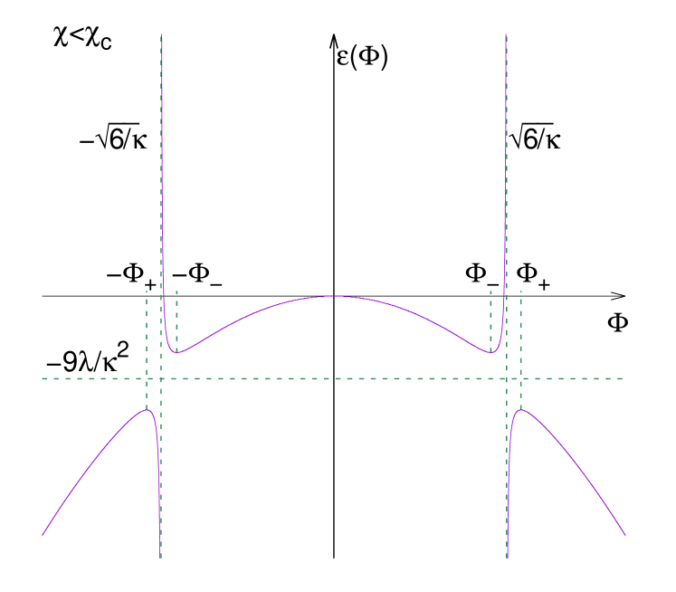
Figure 1: The energy density $\varepsilon$ as a function of the real Higgs field $\Phi$ with $\Pi=0$ and given $\chi^{2}<\chi^{2}_{c}$. $\varepsilon(\Phi)$ has the ‘wine bottle’ (rather than the familiar ‘Mexican hat’) shape, in particular it has minima at $\pm\Phi_{-}$, only in the domain $\Phi^{2}<6/\kappa$. The critical points $\pm\Phi_{+}$ are maxima of $\varepsilon$. If $\chi\rightarrow\chi_{c}$, then $\Phi_{\pm}\rightarrow\sqrt{6/\kappa}$ and $\varepsilon(\Phi_{\pm})\rightarrow-9\lambda/\kappa^{2}$. $\varepsilon(\Phi)$ is singular at $\Phi=\pm\sqrt{6/\kappa}$.

If $\chi\geq\chi_{c}$, then $\varepsilon(\Phi,0,\chi)$, as a function of $\Phi$, is not bounded from below (Fig. 2, Fig. 3). (For a more detailed discussion of the function $\varepsilon=\varepsilon(\Phi,\Pi,\chi)$, see [12].)

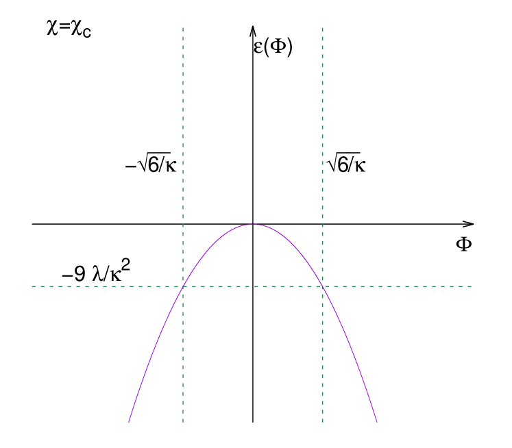
Figure 2: The energy density $\varepsilon$ as a function of the real Higgs field $\Phi$ with $\Pi=0$ and $\chi^{2}=\chi^{2}_{c}$. $\varepsilon(\Phi)$ is not bounded from below.

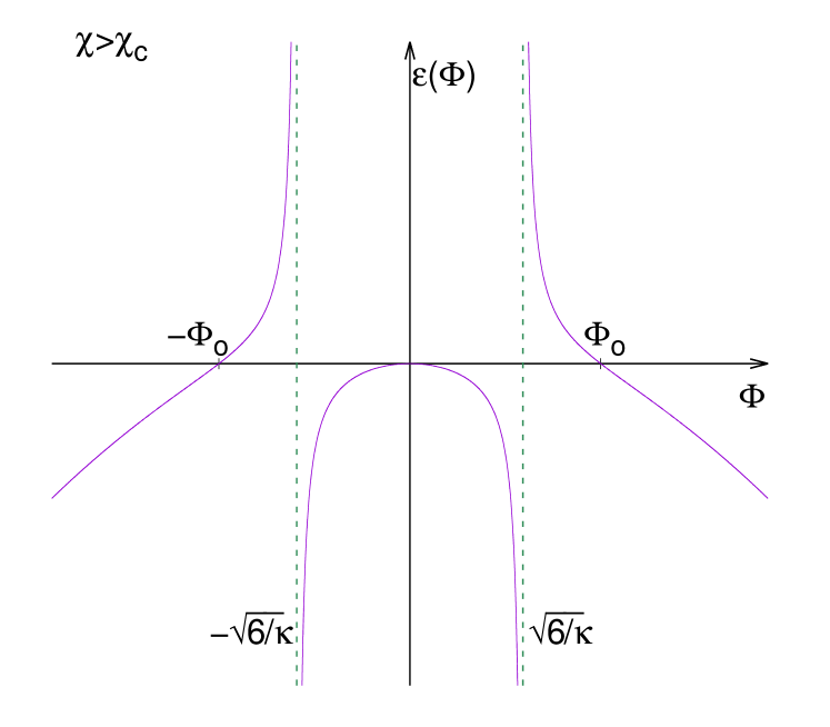
Figure 3: The energy density $\varepsilon$ as a function of the real Higgs field $\Phi$ with $\Pi=0$ and given $\chi^{2}>\chi^{2}_{c}$. $\varepsilon(\Phi)$ is not bounded from below. If $\chi\rightarrow\chi_{c}$, then the zero $\Phi_{0}$ tends to $\sqrt{6/\kappa}$. $\varepsilon(\Phi)$ is singular at $\Phi=\pm\sqrt{6/\kappa}$.

3.3 The instantaneous vacuum states

An instantaneous state of the physical system, represented by tensor fields on a spacelike hypersurface $\Sigma$ defining the ‘instant’, will be called an instantaneous vacuum state if the matter fields admit the isometries of the spacetime as symmetries, solve all the constraint parts of the field equations and minimize the energy functional. Thus, in particular, the instantaneous vacuum states are required to be physical states, i.e. points of the constraint surface in the phase space of the coupled matter+gravity system. Next we determine these states on the transitivity hypersurfaces in the FRW cosmological spacetimes. (For a more detailed discussion of this concept of vacuum state in classical field theory, as well as its particular form in the presence of the Kantowski–Sachs symmetries, representing e.g. the spacetime geometry inside spherical black holes, see [12].)

By (3.5), on a given transitivity hypersurface $\Sigma_{t}$ of the FRW symmetries the energy density can have local minima precisely when the mean curvature of $\Sigma_{t}$ satisfies the inequality $\chi^{2}<\chi^{2}_{c}$. Thus, instantaneous vacuum states cannot exist on hypersurfaces whose mean curvature is the critical value $\chi_{c}$ or higher. Since near the initial singularity of spacetime the mean curvature of the foliation $\Sigma_{t}$ diverges,

$$\chi^{2}<\chi^{2}_{c}:=9\bigl{(}\mu^{2}+\frac{\Lambda}{3}+3\frac{\lambda}{\kappa}\bigr{)}\simeq 4.9\times 10^{64}cm^{-2}$$ (3.6)

is a non-trivial necessary condition for the existence of an instantaneous vacuum state. (In particular, for $\chi^{2}>\chi^{2}_{c}$ the expression under the square root in (3.5) would be negative. The numerical value of $\chi^{2}_{c}$ in (3.6) is given in the $\hbar=c=1$ units.) If such a vacuum state exists, then it is necessarily gauge symmetry breaking (see Fig. 1), and depends on $\chi$. Indeed, $|\Phi_{v}|$ is completely determined by $\chi$, but the $U(1)$ gauge transformation $\Phi_{v}\mapsto\exp({\rm i}\alpha)\Phi_{v}$, $\alpha\in[0,2\pi)$, takes an instantaneous vacuum state into a different such state. Therefore, the instant when the mean curvature is just the critical value $\chi_{c}$ will be the instant of the ‘genesis’/‘evanescence’ of rest masses, just when the BEH mechanism starts/ends to work (depending on whether the mean curvature is decreasing or increasing, respectively). As we will see, the time dependence of $\chi$ yields time dependence of the rest masses obtained via the BEH mechanism.

Since the instantaneous vacuum states are defined to be certain physical states, the corresponding field configuration must solve the Hamiltonian constraint. (The Gauss and the momentum constraints are satisfied identically.) If ${\cal R}_{v}$ denotes the curvature scalar of the intrinsic spatial geometry of the hypersurface $\Sigma_{t}$ in the vacuum state, then, by (3.4), it is

$$\frac{1}{2}{\cal R}_{v}=\Lambda-\frac{1}{4}\kappa\lambda|\Phi_{v}|^{4}-\frac{1}{3}\chi^{2}=\frac{1}{1-\frac{1}{12}\kappa|\Phi_{v}|^{2}}\bigl{(}\Lambda+\frac{1}{4}\kappa\mu^{2}|\Phi_{v}|^{2}-\frac{1}{3}\chi^{2}\bigr{)},$$ (3.7)

which is constant on $\Sigma_{t}$. By (3.5) the first two terms together in the brackets on the right is negative for any $\chi^{2}\leq\chi^{2}_{c}$, and hence ${\cal R}_{v}$ must be negative. Since ${\cal R}=6k/S^{2}$, this implies that the discrete parameter $k$ must be $-1$, and that the value $S_{v}$ of the scale function $S$ is also determined completely by $\chi$. Therefore, in particular, in globally defined instantaneous vacuum states on $\Sigma_{t}$ which would also be invariant with respect to the isometries the intrinsic geometry of $\Sigma_{t}$ is hyperbolic: $k=-1$. In particular, the existence of such states requires that topologically $\Sigma_{t}$ be $\mathbb{R}^{3}$.

On the other hand, if these states were required to be defined only on proper open subsets of $\Sigma_{t}$ and their invariance under the whole isometry group were not required but were allowed to be $O(1,3)$-invariant even in the $k=1,0$ cases, then the existence of these states would not imply $k=-1$. These quasi-locally defined instantaneous (gauge symmetry breaking) vacuum states would be enough to be able to define rest masses quasi-locally, and the non-zero rest masses could in fact be introduced via the BEH mechanism (see also subsections 1.1 and 1.2).

Finally, it should be noted that the 1-parameter family of instantaneous vacuum states, parametrized by the mean curvature $\chi$, does not solve the evolution equations, the second of (3.1) and (3.2): Substituting (3.5) into the evolution equations a tedious but straightforward calculation yields the contradiction $\Phi_{v}=0$. Therefore, the evolution equations take an instantaneous vacuum state into a non-vacuum state in the next instant.

4 The genesis of the rest masses

4.1 The strategy of the calculation of the rest masses

Our calculation of the rest masses via the BEH mechanism is based on the use of the instantaneous vacuum states. Thus we should assume that the spacetime satisfies those conditions that ensure the existence of the instantaneous vacuum states. In particular, the spacetime should admit a foliation by Cauchy surfaces $\Sigma_{t}$ with constant mean curvature, and that the mean curvature can be used as an extrinsic time coordinate (the ‘York time’), by means of which the hypersurfaces can also be labeled. Nevertheless, no evolution equation will be used in these calculations.

To ensure the existence of instantaneous vacuum states, condition (3.6) is assumed to be satisfied. Then the instantaneous vacuum states are necessarily gauge symmetry breaking, and hence the BEH mechanism works. On the other hand, since the rest masses can be introduced even quasi-locally (see subsection 1.1), the instantaneous vacuum states are not required to be global and the BEH mechanism still works.

4.2 The BEH mechanism in the EccHM system

Suppose that the leaves $\Sigma_{t}$ of the foliation are of constant mean curvature. Let us choose the vacuum state, $\Phi_{v}$, to be real. Then by an appropriate gauge transformation any Higgs field can be transformed into the form $\Phi=\Phi_{v}+H$, where $H$ is a real function. In fact, the existence of such a gauge (the so-called ‘unitary gauge’) is a consequence of a much more general result, proven by Weinberg, even for arbitrary Higgs multiplet and any compact gauge group [17]. Then, in this gauge, the matter sector of the instantaneous vacuum states is characterized by $\phi=0$, $A_{a}=0$, $H=0$ and $E_{a}=0$, $\dot{H}=0$, $\Pi=0$. The latter implies that $t^{a}\nabla_{a}\Phi_{v}=-\frac{1}{3}\chi\Phi_{v}$. Note that, in the gravitational sector of the instantaneous vacuum states, the extrinsic curvature is a pure trace: $\chi_{ab}=\frac{1}{3}\chi h_{ab}$.

Rewriting the Lagrangian density $\hat{\cal L}:=\hat{\cal L}_{H}+{\cal L}_{M}$ in terms of the variables $\phi$, $A_{a}$, $H$ and their time derivative, its derivative with respect to the gauge potentials (while keeping their derivatives fixed) at the instantaneous vacuum state are

$$\bigl{(}\frac{\partial\hat{\cal L}}{\partial\phi}\bigr{)}_{v}=\bigl{(}\frac{\partial\hat{\cal L}_{H}}{\partial\phi}\bigr{)}_{v}=\frac{\rm i}{2}\Bigl{(}\Phi t^{c}{\nabla\!\!\!\!/}_{c}\bar{\Phi}-\bar{\Phi}t^{c}{\nabla\!\!\!\!/}_{c}\Phi\Bigr{)}_{v}=0,$$

$$\bigl{(}\frac{\partial\hat{\cal L}}{\partial A_{a}}\bigr{)}_{v}=\bigl{(}\frac{\partial\hat{\cal L}_{H}}{\partial A_{a}}\bigr{)}_{v}=\frac{\rm i}{2}\Bigl{(}\Phi\mathbb{D}^{a}\bar{\Phi}-\bar{\Phi}\mathbb{D}^{a}\Phi\Bigr{)}_{v}=0.$$

Here, in the first equation we used that in the vacuum state $E_{a}=0$, $D_{a}\Phi_{v}=0$ and $\Pi_{v}=0$; while in the second that $A_{a}=0$ and $D_{a}\Phi_{v}=0$. These two equations can be summarized as $(\partial\hat{\cal L}/\partial\omega_{a})_{v}=((\partial\hat{\cal L}/\partial\phi)t^{a}+(\partial\hat{\cal L}/\partial A_{b})P^{a}_{b})_{v}=0$. The first derivative of $\hat{\cal L}$ with respect to $\Phi$ (while keeping $\dot{\Phi}$ and $D_{a}\Phi$ fixed) at the instantaneous vacuum state is

$$\bigl{(}\frac{\partial\hat{\cal L}}{\partial\Phi}\bigr{)}_{v}\!\!\!\! =\!\!\!\! -\frac{1}{2}\mu^{2}\Phi_{v}-\frac{1}{2}\lambda\Phi^{3}_{v}-\frac{1}{12}\bigl{(}{\cal R}_{v}+\chi_{ab}\chi^{ab}-\chi^{2}\bigr{)}\Phi_{v}-\frac{1}{18}\chi^{2}\Phi_{v}=$$

$$=\!\!\!\! -\frac{1}{2}\Bigl{(}\frac{1}{6}\bigl{(}{\cal R}_{v}+\chi^{2}-\chi_{ab}\chi^{ab}\bigr{)}+\mu^{2}+\lambda|\Phi_{v}|^{2}-\frac{1}{9}\chi^{2}\Bigr{)}\Phi_{v}=$$

$$=\!\!\!\! -\frac{1}{2}\Bigl{(}-\frac{1}{12}\kappa\lambda|\Phi_{v}|^{4}+\lambda|\Phi_{v}|^{2}+\mu^{2}+\frac{1}{3}\Lambda-\frac{1}{9}\chi^{2}\Bigr{)}\Phi_{v}=0.$$

Here, in the second step we used $\chi_{ab}=\chi h_{ab}/3$, in the third step the Hamiltonian constraint and the expression of the energy density $\varepsilon_{v}(\chi)$ in the vacuum state (see subsection 3.2), and in the last step (3.4). This yields

$$\bigl{(}\frac{\partial\hat{\cal L}}{\partial H}\bigr{)}_{v}=\Bigl{(}\frac{\partial\hat{\cal L}}{\partial\Phi}+\frac{\partial\hat{\cal L}}{\partial\bar{\Phi}}\Bigr{)}_{v}=0.$$

Therefore, the instantaneous vacuum state is a critical point of the Lagrangian $\hat{\cal L}$ both with respect to the gauge and the Higgs fields, and hence their rest mass is well defined. In fact, the rest mass for the gauge field,

$$m^{2}_{\omega}:=\frac{1}{4}\bigl{(}g_{ab}\frac{\partial^{2}\hat{\cal L}}{\partial\omega_{a}\partial\omega_{b}}\bigr{)}_{v}=\frac{1}{4}\bigl{(}g_{ab}\frac{\partial^{2}\hat{\cal L}_{H}}{\partial\omega_{a}\partial\omega_{b}}\bigr{)}_{v}=\Phi_{v}^{2},$$ (4.1)

is well defined and positive. To calculate the rest mass for $H$, first we compute the second derivatives of $\hat{\cal L}_{H}$ with respect to $\Phi$ and $\bar{\Phi}$:

$$\bigl{(}\frac{\partial^{2}\hat{\cal L}_{H}}{\partial\Phi^{2}}\bigr{)}_{v}\!\!\!\! =\!\!\!\! -\frac{1}{2}\lambda\Phi^{2}_{v},$$

$$\bigl{(}\frac{\partial^{2}\hat{\cal L}_{H}}{\partial\Phi\partial\bar{\Phi}}\bigr{)}_{v}\!\!\!\! =\!\!\!\! -\frac{1}{2}\mu^{2}-\lambda\Phi_{v}^{2}-\frac{1}{12}\bigl{(}{\cal R}_{v}+\chi^{2}-\chi_{ab}\chi^{ab}\bigr{)}+\frac{1}{9}\chi^{2}=$$

$$=\!\!\!\! -\frac{1}{2}\Bigl{(}-\frac{1}{12}\kappa\lambda\Phi_{v}^{4}+2\lambda\Phi_{v}^{2}+\mu^{2}+\frac{1}{3}\Lambda-\frac{2}{9}\chi^{2}\Bigr{)}=-\frac{1}{2}\bigl{(}\lambda\Phi_{v}^{2}-\frac{1}{9}\chi^{2}\bigr{)}.$$

Thus, finally, the rest mass of the field $H$ is

$$m^{2}_{H}:=-\bigl{(}\frac{\partial^{2}\hat{\cal L}}{\partial H^{2}}\bigr{)}_{v}=-\Bigl{(}\frac{\partial^{2}\hat{\cal L}_{H}}{\partial\Phi^{2}}+2\frac{\partial^{2}\hat{\cal L}_{H}}{\partial\Phi\partial\bar{\Phi}}+\frac{\partial^{2}\hat{\cal L}_{H}}{\partial\bar{\Phi}^{2}}\Bigr{)}_{v}=2\lambda\Phi_{v}^{2}-\frac{1}{9}\chi^{2}.$$ (4.2)

Since, to guarantee the existence of instantaneous vacuum states we assumed that $\chi^{2}<\chi^{2}_{c}$, by (3.5) the rest mass of the field $H$ is positive.

4.3 The time dependence of the rest masses

By (3.5) the norm $|\Phi_{v}|$ depends on the mean curvature, and hence the rest masses $m_{\omega}$ and $m_{H}$ are time dependent if $\dot{\chi}\not=0$, though they have different time dependence. In particular, both are monotonically decreasing with decreasing $\chi^{2}$. At the instant of their ‘genesis’, i.e. in the $\chi^{2}\rightarrow\chi^{2}_{c}$ limit, $m^{2}_{\omega}\rightarrow 3/\kappa$ and $m^{2}_{H}\rightarrow 9\lambda/\kappa-\mu^{2}-\Lambda/3\simeq 1.7\times 10^{64}cm^{-2}$ (in the $\hbar=c=1$ units).

Since $({\rm d}|\Phi_{v}|^{2}/{\rm d}\chi^{2})$ diverges if $\chi^{2}\rightarrow\chi^{2}_{c}$ and $({\rm d}|\Phi_{v}|^{2}/{\rm d}\chi^{2})\rightarrow 0$ if $\chi\rightarrow 0$, the time dependence of the rest masses is significant only just after their ‘genesis’. For example, while the Hubble time corresponding to $\chi_{c}$ is $t_{c}:=3/\chi_{c}\simeq 4.5\times 10^{-43}sec$ (which is almost ten Planck times), the Higgs mass decreased to the half of its initial value (at the instant of its ‘genesis’) by $5.8\times 10^{-43}sec$ Hubble time (i.e. c.c. in the next three Planck times); and it decreased to twice of its present value, viz. to $2\times(6.2\times 10^{15}cm^{-1})$, by $5.5\times 10^{-26}sec$ Hubble time. Remarkably enough, the characteristic time of the weak interactions that the Higgs mass parameter defines is $1/c|\mu|\simeq 5.4\times 10^{-27}sec$. Hence, at this characteristic time, the rest mass of the Higgs field was roughly twice of its present value.

On the other hand, for small enough $\chi^{2}$ the norm $|\Phi_{v}|$ can be expanded as

$$|\Phi_{v}|^{2}=\frac{6}{\kappa}\Bigl{(}1-\sqrt{1+\frac{\kappa}{3\lambda}(\mu^{2}+\frac{1}{3}\Lambda-\frac{1}{9}\chi^{2})}\Bigr{)}=-\frac{\mu^{2}}{\lambda}+\frac{\kappa}{12}\frac{\mu^{4}}{\lambda^{2}}-\frac{1}{3\lambda}\bigl{(}\Lambda-\frac{1}{3}\chi^{2}\bigr{)}+....$$ (4.3)

The first term in the expansion is the well known vacuum value in the Standard Model in Minkowski spacetime (see e.g. [6]), the second, being proportional to Newton’s gravitational constant, is of proper gravitational origin, while the third, containing the cosmological constant and the rate of expansion of the universe, has cosmological origin. In the $\chi^{2}\rightarrow 0$ limit $|\Phi_{v}|^{2}$ reduces to that obtained in subsection 2.2 for the norm of the Higgs field in the ‘spacetime vacuum state’ (see equation (2.10)). The present value of the Hubble constant in our observed Universe is $(\dot{S}/S)_{\rm now}=\frac{1}{3}\chi_{\rm now}\simeq 7\times 10^{-28}cm^{-1}$. Hence, the corrections in (4.3) to the value $\sqrt{-\mu^{2}/\lambda}$ of the norm of the Higgs field in the symmetry breaking vacuum state in the Poincaré invariant Standard Model are extremely tiny, and they have significance only in the extreme gravitational circumstances.

5 Summary, conclusions and final remarks

We investigated certain kinematical consequences of the conformally invariant coupling of the Higgs field to Einstein’s theory of gravity. First, we showed that global spacetime vacuum states, i.e. which would have maximal spacetime symmetry, solve the field equations and minimize the energy density, do not exist. Then, we showed that in the $k=0,1$ FRW spacetimes global instantaneous vacuum states, i.e. field configurations on the transitivity hypersurfaces of the spacetime symmetries which would be invariant with respect to these symmetries, solve the constraint parts of the field equations and minimize the energy functional, do not exist. Also, even general quasi-local instantaneous vacuum states (i.e. which are represented by field configurations that are not necessarily globally defined on the spacelike hypersurfaces) do not exist on hypersurfaces whose mean curvature is greater than a large, but finite critical value. If the mean curvature is less than this critical value, then instantaneous vacuum states exist, which are necessarily gauge symmetry breaking and depend on the mean curvature.

Using this concept of the global or quasi-local instantaneous (gauge symmetry breaking) vacuum states, in spacetimes that admit a foliation by constant mean curvature Cauchy hypersurfaces and the mean curvature can be used as a time coordinate, we determined how the rest mass of the matter fields of the Einstein-conformally coupled Higgs-Maxwell system depends on the extrinsic York time parameter of the hypersurfaces. We found that there are extreme gravitational situations in which the notion of rest mass of the Higgs field, zero or non-zero, cannot be introduced. In these situations the Higgs field does not have particle interpretation. The resulting non-zero rest masses of the fields, introduced via the BEH mechanism, are time dependent in a non-stationary spacetime and they are decreasing with decreasing mean curvature.

Therefore, according to the present model, the scenario of the genesis of the observed non-zero rest mass of the fields is rather different from the usual view: According to the traditional picture initially, in the very early stage of the history of the Universe, the Higgs field was in the symmetric vacuum state and the gauge and the fermion fields had zero rest mass, and at a (mathematically still not yet specified) later stage the Higgs field developed into a symmetry braking vacuum and the gauge and fermion fields got non-zero rest mass via the BEH mechanism. On the other hand, according to the present model, initially the Higgs field did not have any vacuum state and its rest mass was not defined at all, while the gauge field had zero rest mass. When the mean curvature decreased below the critical value, symmetry breaking vacuum states of the Higgs field emerged, and the gauge and the Higgs fields got enormously large rest masses. These rest masses were decreasing rapidly to their present value with the expansion of the Universe.

In fact, the key statements in the present simple model hold true in the more realistic Einstein-conformally coupled Standard Model (EccSM) system, in which the gauge group could be any compact Lie group, the Higgs field is a multiplet of complex self-interacting fields and there could be any collection of Weyl spinor fields coupled in the minimal way to the gauge fields and via the Yukawa coupling to the Higgs multiplet [12]. In particular, in the Einstein-conformally coupled Weinberg–Salam model the rest mass of the electron, and the W and Z bosons is $m_{e}=\frac{1}{\sqrt{2}}G_{e}|\Phi_{v}|$, $m_{W}=\frac{1}{2}g|\Phi_{v}|$, $m_{Z}=\frac{1}{2}\sqrt{g^{2}+g^{\prime}{}^{2}}|\Phi_{v}|$, respectively. Here $G_{e}$ is the appropriate Yukawa coupling, and $g$ and $g^{\prime}$ are the $SU(2)$ and $U(1)$ coupling constants, respectively. Thus all of these have the same time dependence via $|\Phi_{v}|$, which is different from that of the Higgs rest mass given by (4.2) above. Since in the Weinberg–Salam model electromagnetism is an emergent phenomenon due to the $U(2)\rightarrow U(1)$ gauge reduction during the symmetry breaking, in the Einstein-conformally coupled Weinberg–Salam model electromagnetism and the electric charge, $|e|=gg^{\prime}(g^{2}+g^{\prime}{}^{2})^{-1/2}$, emerge at the same instant when the rest masses, at $\chi=\chi_{c}$. On the other hand, contrary to the non-zero rest masses, the charge $e$ does not depend on $\chi$.

If the mean curvature of the hypersurfaces happened to be increasing and exceeded the critical value, then the massive fields would lose their rest mass. In our (asymptotically exponentially expanding) Universe the mean curvature asymptotically tends to the finite, constant value $\sqrt{\Lambda/3}$. Hence the ‘reverse–BEH’ mechanism at the cosmological scale cannot provide the way in which the fields lose their rest mass. The ‘reverse-BEH’ mechanism takes place inside black holes, deeply behind the event horizon near the central singularity. In fact, the specific analysis of section 3 can be carried out in the presence of Kantowski–Sachs (rather than FRW) symmetries, describing the spacetime geometry inside spherical black holes, and one can determine the (quasi-local) instantaneous vacuum states and calculate the rest masses [12]. The matter fields falling into a spherical black hole loose their rest mass before hitting the central singularity.

The time dependence (and the different time dependence) of the Higgs and the other fields is significant only when the mean curvature is close to its critical value. Thus, it may have a potential significance in the particle physics processes in the very early Universe (or near the central singularity in spherical black holes). Hence it could be interesting to see whether or not this time dependence, and in particular the fact that at the characteristic time scale defined by the Higgs rest mass parameter the rest masses were twice their present value, could yield observable effect in the particle genesis era of the very early Universe.

The author is grateful to Árpád Lukács, Péter Vecsernyés and György Wolf for the numerous and enlightening discussions both on the structure of the Standard Model and on various aspects of the present suggestion. Special thanks to György Wolf for the careful reading of an earlier version of the paper, his suggestions to improve the text at several points and for drawing the figures; and to Helmut Friedrich and Paul Tod for their remarks on both the conformal cyclic cosmological model and the present suggestions. Thanks are due to the ‘Geometry and Relativity’ program at the Erwin Schrödinger International Institute for Mathematics and Physics, Vienna, for the support and hospitality where the final version of the present paper was prepared.

References

- [1] R. Penrose, Cycles of Time, The Bodley Head, London 2010, ISBN 9780224080361
- [2] V. I. Arnold, Mathematical Methods of Classical Mechanics, Springer 1989, ISBN 0-387-96890-3
- [3] S. W. Hawking, G. F. R. Ellis, The Large Scale Structure of Spacetime, Cambridge University Press, Cambridge 1973, ISBN 0-521-09906-4
- [4] R. W. Higgs, Broken symmetries and the masses of gauge bosons, Phys. Rev. Lett. 13 508-509 (1964), doi: 10.1103/PhysRevLett.13.508
- [5] F. Englert, R. Brout, Broken symmetry and the mass of gauge vector mesons, Phys. Rev. Lett. 13 321-323 (1964), doi: 10.1103/PhysRevLett.13.321
- [6] E. S. Abers, B. W. Lee, Gauge theories, Phys. Rep. 9 1–141 (1973), doi: 10.1016/0370-1573(73)90027-6 T.-P. Cheng, L.-F. Li, Gauge Theory of Elementary Particle Physics, Clarendon Press, Oxford 1984, ISBN 0-19-851961-3
- [7] R. Penrose, W. Rindler, Spinors and Spacetime, vol 1, Cambridge University Press, Cambridge 1982, ISBN 0-521-24527-3
- [8] J. D. Bjorken, S. D. Drell, Relativistic Quantum Mechanics, McGraw-Hill Book Co, Yew York 1964, ISBN 07-005493-2
- [9] S. W. Hawking, Stable and generic properties in general relativity, Gen. Relat. Grav. 1 393-400 (1971), doi: 10.1007/BF00759218
- [10] R. A. Adams, J. J. F. Fournier, Sobolev Spaces, Academic Press, Amsterdam 2003, ISBN: 0-12-044143-8
- [11] R. Penrose, M. A. H. MacCallum, Twistor theory: An approach to the quantisation of fields and space-time, Phys. Rep. 6 241-316 (1972), doi:10.1016/0370-1573(73)90008-2
- [12] L. B. Szabados, Gravity, as a classical regulator for the Higgs field, and the genesis of rest masses and charge, arXiv: 1603.06997v3 [gr-qc]
- [13] I. Agullo, W. Nelson, A. Ashtekar, Preferred instantaneous vacuum for linear scalar fields in cosmological space-times, Phys. Rev. D 91 064051 (2015), doi: 10.1103/PhysRevD.91.064051, arXiv: 1412.3524v2 [gr-qc]
- [14] E. T. Newman, R. Penrose, New conservation laws for zero rest-mass fields in asymptotically flat spacetimes, Proc. Roy. Soc. A 305 175-204 (1968), doi: 10.1098/rspa.1968.0112
- [15] L. B. Szabados, Gy. Wolf, Singularities in Einstein-conformally coupled Higgs cosmological models, arXiv: 1802.00774 [gr-qc]
- [16] J. Isenberg, J. Nester, Canonical gravity, in General Relativity and Gravitation, Vol 1, Ed. A. Held, Plenum Press, New York 1980, ISBN 0-306-40365-3(v.1)
- [17] S. Weinberg, General theory of broken local symmetry, Phys. Rev. D 7 1068-1082 (1973), doi: 10.1103/PhysRevD.7.1068