Efficient Model–Based Deep Reinforcement Learning with
Variational State Tabulation
Abstract
Modern reinforcement learning algorithms reach super–human performance on many board and video games, but they are sample inefficient, i.e. they typically require significantly more playing experience than humans to reach an equal performance level. To improve sample efficiency, an agent may build a model of the environment and use planning methods to update its policy. In this article we introduce Variational State Tabulation (VaST), which maps an environment with a high–dimensional state space (e.g. the space of visual inputs) to an abstract tabular model. Prioritized sweeping with small backups, a highly efficient planning method, can then be used to update state–action values. We show how VaST can rapidly learn to maximize reward in tasks like 3D navigation and efficiently adapt to sudden changes in rewards or transition probabilities.
- RL
- Reinforcement Learning
- VaST
- Variational State Tabulation
- MFEC
- Model–Free Episodic Control
- NEC
- Neural Episodic Control
- MDP
- Markov Decision Process
- POMDP
- partially–observable Markov Decision Process
- CNN
- Convolutional Neural Network
- DCNN
- Deconvolutional Neural Network
- VAE
- Variational Autoencoder
- LSH
- Locality Sensitive Hashing
1 Introduction
Classical Reinforcement Learning (RL) techniques generally assume a tabular representation of the state space (Sutton & Barto, 2018). While methods like prioritized sweeping (Sutton & Barto, 2018; Moore & Atkeson, 1993; Peng & Williams, 1993; Van Seijen & Sutton, 2013) have proven to be very sample–efficient in tabular environments, there is no canonical way to carry them over to very large (or continuous) state spaces, where the agent seldom or never encounters the same state more than once. Recent approaches to reinforcement learning have shown tremendous success by using deep neural networks as function approximators in such environments, allowing for generalization between similar states (e.g. Mnih et al. (2015, 2016)) and learning approximate dynamics to perform planning at decision time (e.g. Silver et al. (2017); Oh et al. (2017); Farquhar et al. (2017); Racanière et al. (2017); Nagabandi et al. (2017)). However, methods like prioritized sweeping that use a model for offline updates of -values (i.e. background planning (Sutton & Barto, 2018)), have not yet been investigated in conjunction with function approximation by neural networks.
Adjusting the weights in a deep network is a slow procedure relative to learning in tabular environments. In particular, agents using deep architectures typically fail to take advantage of single experiences that significantly alter the policy. This was illustrated by recent work on Model–Free Episodic Control (MFEC) (Blundell et al., 2016), where a very simple agent using a semi–tabular approach significantly outperformed existing deep network approaches in the early stages of learning. The basic MFEC agent uses a random projection from the observation space to a low–dimensional space, and stores the discounted returns associated with observations in a lookup table. The -values of states observed for the first time are determined by a k–Nearest–Neighbour average over discounted returns associated with similar existing states in the lookup table.
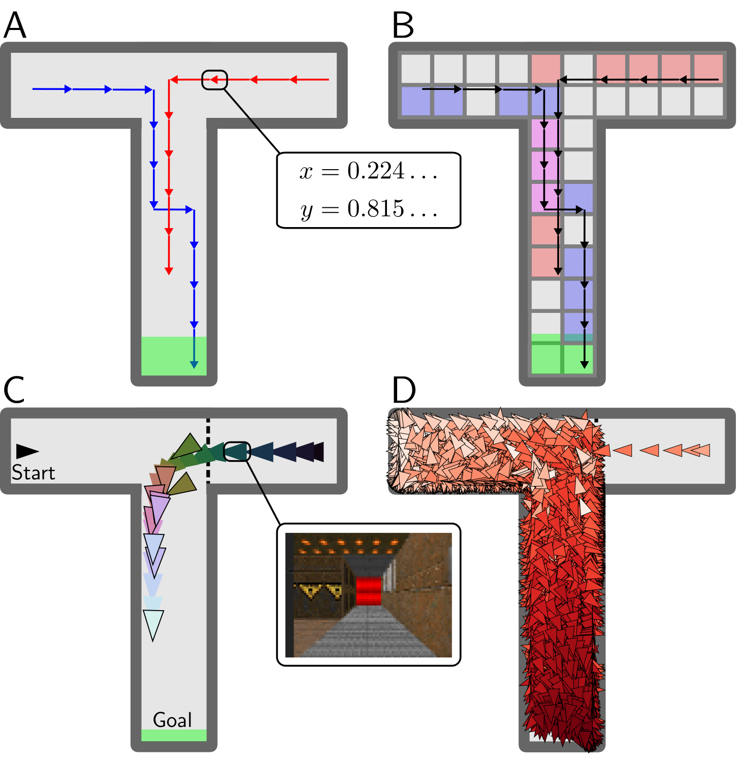
As an example with an MFEC agent, we can consider the T–maze task shown in Figure 1A. The observations are continuous coordinates; the agent can take a fixed–sized step in one of four cardinal directions, with a rebound on hitting a wall, and a terminal reward zone (green). The first episode (red) is spontaneously terminated without reward; the discounted returns along the red trajectory are therefore set to zero. On the second episode (blue), the agent reaches the reward zone, and the discounted reward is immediately associated with the states visited along the blue trajectory.
To improve sample efficiency, we consider how an agent could apply the experience of the rewarded trajectory to -value estimates in the top–right arm. In particular, by learning a model of the environment, the agent could learn that both trajectories pass through the center of the T–maze, and that discovering a reward at the bottom of the maze should therefore change -value estimates in both of the arms at the top. This idea is exploited by the model–based RL technique of prioritized sweeping (Moore & Atkeson, 1993; Peng & Williams, 1993; Van Seijen & Sutton, 2013).
However, assuming random restarts, the agent in this task never encounters the same state more than once. In this case, given a deterministic task, prioritized sweeping as implemented by Van Seijen & Sutton (2013) collapses to the MFEC learning algorithm (Brea, 2017). We are therefore motivated to consider mapping the observation space to a tabular representation by some form of discretisation. For example, with discretisation based on rounding the coordinates (a simple form of state aggregation (Li et al., 2006; Sutton & Barto, 2018)), the two trajectories in Figure 1B now pass through several of the same states. A model–based prioritized sweeping algorithm would allow us to update the -values in the top–right arm of the maze to nonzero values after experiencing both episodes, despite the fact that the red trajectory did not result in reward.
If observations are given by high-dimensional visual inputs instead of coordinates, the simple form of state aggregation by rounding (Figure 1B) is impractical. Instead, we propose and describe in this article the new method of Variational State Tabulation (VaST)111The full code for VaST can be found at https://github.com/danecor/VaST/. for learning discrete, tabular representations from high–dimensional and/or continuous observations. VaST can be seen as an action conditional hybrid ANN–HMM (artificial neural network hidden Markov model, see e.g. (Bengio et al., 1992; Tucker et al., 2017; Ng et al., 2016; Maddison et al., 2016)) with a -dimensional binary representation of the latent variables, useful for generalization in RL. VaST is trained in an unsupervised fashion by maximizing the evidence lower bound. We exploit a parallelizable implementation of prioritized sweeping by small backups (Van Seijen & Sutton, 2013) to constantly update the value landscape in response to new observations. By creating a tabular representation with a dense transition graph (i.e. where the same state is revisited multiple times), the agent can rapidly update state–action values in distant areas of the environment in response to single observations.
In Figure 1C&D, we show how VaST can use the generalization of the tabular representation to learn from single experiences. We consider a 3D version of the example T–maze, implemented in the VizDoom environment (Kempka et al., 2016). Starting from the top–left arm, the agent was trained to run to a reward in the bottom of the T–maze stem. During training, the top–right arm of the T–maze was blocked by an invisible wall. After training, the agent observed a single, 20–step fixed trajectory (or “forced run”) beginning in the top–right arm and ending in the stem, without reaching the reward zone (Figure 1C). The agent’s early observations in the unexplored right arm were mapped to new states, while the observations after entering the stem were mapped to existing states (corresponding to observations at similar positions and orientations). The agent was able to update the values of the new states by prioritized sweeping from the values of familiar states (Figure 1D), without needing to change the neural network parameters, as would be necessary with model-free deep reinforcement learners like DQN (Mnih et al., 2013).
2 Learning the Model
In order to compute a policy using the model–based prioritized sweeping algorithm described by Van Seijen & Sutton (2013), we seek a posterior distribution over latent discrete states given a causal filter over recent observations . We use a variational approach to approximate this posterior distribution.
2.1 The variational cost function
For a sequence of states and observations , we consider a family of approximate posterior distributions with parameters , which we assume to factorise given the current observation and a memory of the past observations, i.e.
| (1) |
where observations before consist of blank frames. To learn , we also introduce an auxiliary distribution parameterized by . Given a collection of observation sequences and hidden state sequences , we maximize the log–likelihood of the weight parameters , while minimizing . Together, these terms form the evidence lower bound (ELBO) or negative variational free energy
| (2) |
where denotes the entropy of the distribution. The term inside the expectation evaluates to
| (3) |
where denotes the action taken by the agent on step of sequence , is the distribution over initial states, and .
We aim to learn the appropriate posterior distribution by minimizing the variational free energy (maximizing the ELBO). Our cost function from Eq. 2.1 can be written as
| (4) |
with reconstruction cost terms
| (5) |
transition cost terms
| (6) |
for and and entropy terms
| (7) |
We parameterize the posterior distribution (or “encoder”) using a deep Convolutional Neural Network (CNN) (Krizhevsky et al., 2012), and the observation model using a deep Deconvolutional Neural Network (DCNN) (Goodfellow et al., 2014), as shown in Figure 2. We use a multilayer perceptron (3 layers for each possible action) for the transition model , and learned parameters for the initial state distribution . The architecture is similar to that of a Variational Autoencoder (VAE) (Kingma & Welling, 2013; Rezende et al., 2014), with the fixed priors replaced by learned transition probabilities conditioned on previous state–action pairs.
To allow for a similarity metric between discrete states, we model the state space as all possible combinations of binary variables, resulting in possible states. Each of the outputs of the encoder defines the expectation of a Bernoulli random variable, with each variable sampled independently. The sampled states are used as input to the observation and transition networks, and as targets for the transition network.
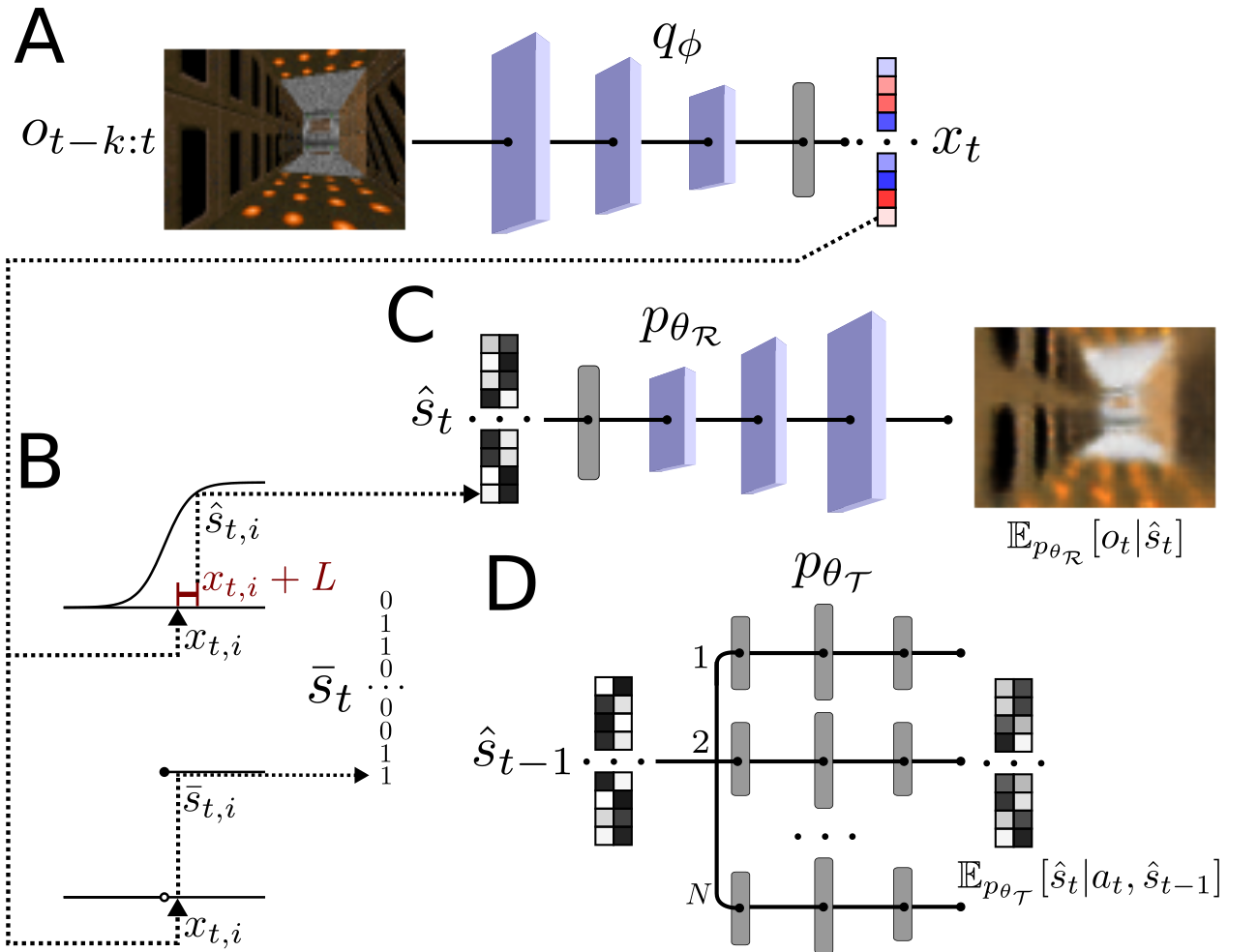
The reconstruction and transition cost terms can now be used in stochastic gradient descent on in , by estimating the gradient with Monte Carlo samples from the variational posterior . To minimize also in , we need to perform backpropagation over discrete, stochastic variables (i.e. over sampled from ). There are several methods for doing this (see Discussion). We use the reparameterization trick together with a relaxation of the Bernoulli distribution: the binary Con–crete (or Gumbel–Softmax) distribution (Maddison et al. (2016); Jang et al. (2016)).
2.2 The reparameterization trick and the Con–crete distribution
Denoting the ith dimension of state as , we consider the ith output of the encoder at time to correspond to . Following Maddison et al. (2016), we note that we can achieve a Bernoulli distribution by sampling according to , where is the Heaviside step function and is a logistic random variable. In this form, the stochastic component is fully independent of , and we can simply backpropagate through the deterministic nodes (Kingma & Welling, 2013). However, the derivative of is almost everywhere. To address this, the Bernoulli distribution can be relaxed into a continuous Con–crete (continuous relaxation of discrete) distribution (Maddison et al., 2016). This corresponds to replacing the Heaviside non–linearity with a logistic non–linearity parameterized by the temperature :
| (8) |
with . We use Con–crete samples from the encoder output for the input to both the reconstruction and transition networks and for the targets of the transition network, with temperatures taken from those suggested in (Maddison et al., 2016): for the posterior distribution and for evaluating the transition log–probabilities. The Con–crete relaxation corresponds to replacing the discrete joint Bernoulli samples in the previous loss functions with their corresponding joint Con–crete samples . We train the network by sampling minibatches of observations and actions from a replay memory (Riedmiller, 2005; Mnih et al., 2015) of transitions observed by the agent.
2.3 Learning a tabular transition model
The model as described learns a joint Con–crete posterior distribution . We can recover a discrete joint Bernoulli distribution by replacing the logistic non–linearity with a Heaviside non–linearity (i.e. as in Eq. 8).
For prioritized sweeping, we need to build a tabular model of the transition probabilities in the environment (i.e. ). We could consider extracting such a model from , the transition network used to train the encoder. However, this is problematic for several reasons. The transition network corresponds to Con–crete states, and is of a particularly simple form, where each dimension is sampled independently conditioned on the previous state and action. Moreover, the transition network is trained through stochastic gradient descent and therefore learns slowly; we want the agent to rapidly exploit new transition observations.
We therefore build a state transition table based purely on the encoder distribution , by treating the most probable sequence of states under this distribution as observed data. Since each dimension of is independent conditioned on the observations, the mode at time corresponds to a –length binary string, where . Likewise, since states within an episode are assumed to be independent conditioned on the causal observation filter, the most probable state sequence for an episode is . We therefore record a transition between and under action for every step taken by the agent, and update the expected reward in the table with the observed reward. Each binary string is represented as a –bit unsigned integer in memory.
This process corresponds to empirically estimating the transition probabilities and rewards by counting, with counts that are revised during training. For instance, assume the agent encounters states , and successively in the environment. We record transitions and in the table, and store the raw observations along with the corresponding state assignments , and in the replay memory. If the observations associated with are later sampled from the replay memory and instead assigned to state , we delete and from the table and add and . Both the deletion and addition of transitions through training can change the -values.
2.4 Using the model for reinforcement learning
The -values in the table are updated continuously using the learned transition model , expected rewards and prioritized sweeping with small backups (Van Seijen & Sutton, 2013). Prioritized sweeping converges to the same solution as value iteration, but can be much more computationally efficient by focusing updates on states where the -values change most significantly.
Given an observation history , the agent follows an –greedy policy using the -values in the lookup table for all possible actions . For any pair that has not yet been observed, we estimate the -value using an experience–weighted average over the nearest neighbours to in Hamming distance (see Supplementary Materials for details). This Hamming neighbour estimate is parameter–less, and generally much faster than searching for nearest neighbours in continuous space.
2.5 Implementation details
The prioritized backups described by Van Seijen & Sutton (2013) are performed serially with environment exploration. To decrease training time and improve performance, we performed backups independently, and in parallel, to environment exploration and training the deep network.
We implemented state tabulation and prioritized sweeping as two separate processes (running on different CPU cores). The tabulation process acts in the environment and trains the neural networks by sampling the replay memory. The sweeping process maintains the transition table and continuously updates the Q-values using prioritized sweeping.
To perform greedy actions, the tabulation process requests -values from the sweeping process. To update the transition table, the tabulation process sends transition updates (additions and deletions) to the sweeping process. Our implementation of the sweeping process performed backups/second, allowing the agent to rapidly propagate -value changes with little effect on the simulation time.
The pseudocode of VaST, and of our implementation of prioritized sweeping, are in the Supplementary Material.
3 Results
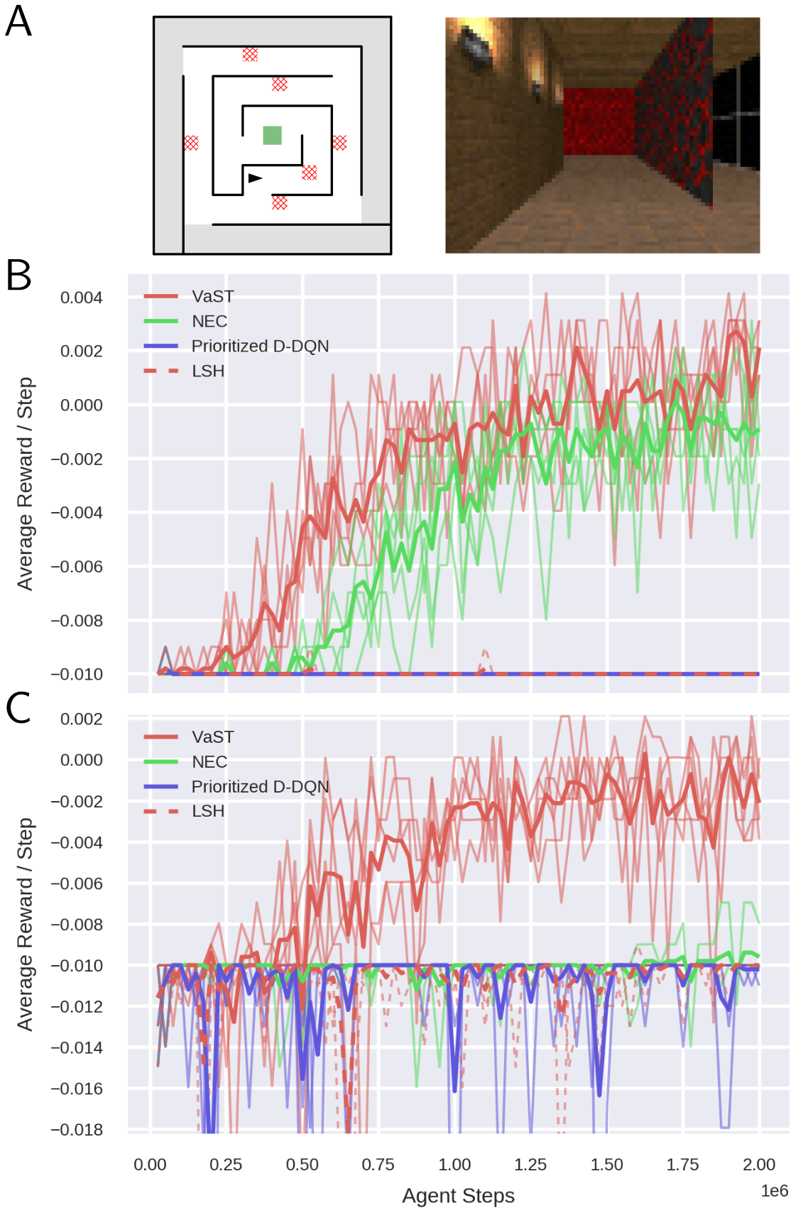
We evaluated the VaST agent on a series of navigation tasks implemented in the VizDoom environment (see Figure 3A, Kempka et al. (2016)). Each input frame consists of a 3–channel pixel image of the 3D environment, collected by the agent at a position and orientation . The agent rarely observes the exact same frame from a previous episode ( – of the time in the mazes used here), making it ill–suited for a traditional tabular approach; yet the discovery of new transitions (particularly shortcuts) can have a significant effect on the global policy if leveraged by a model–based agent. We considered the relatively low–data regime (up to 2 million steps). Three actions were available to the agent: move forward, turn left and turn right; due to momentum in the game engine, these give rise to visually smooth trajectories. We also trained the agent on the Atari game Pong (Figure 7). For 3D navigation, we used only the current frame as input to the network, while we tested both 1– and 4–frame inputs for Pong.
We compared the performance of VaST against two recently published sample–efficient model–free approaches: Neural Episodic Control (NEC) (Pritzel et al., 2017) and Prioritized Double–DQN (Schaul et al., 2015). We used the structure of the DQN network in (Mnih et al., 2015) for both NEC and Prioritized D–DQN as well as the encoder of VaST (excluding the output layers). Full hyperparameters are given in the Supplementary Material.
We also compared against prioritized sweeping using Locality Sensitive Hashing (LSH) with random projections (Charikar, 2002), where each bit , and each fixed projection vector had elements sampled from at the beginning of training. The environment model and -values were determined as with VaST.
In the first task (Figure 3), the agents were trained to reach a reward of +1 in the center of a complex maze, starting from a random position and orientation in the outer region. In a second version of the task, we added six “hazard” regions which gave a penalty of -1 with a probability of for each step. The agents were evaluated over a 1000–step test epoch, with , every 25 000 steps. VaST slightly outperformed NEC on the first version of the task and significantly outperformed all of the other models on the more difficult version (Figure 3C).
3.1 Dimensionality of the latent representation
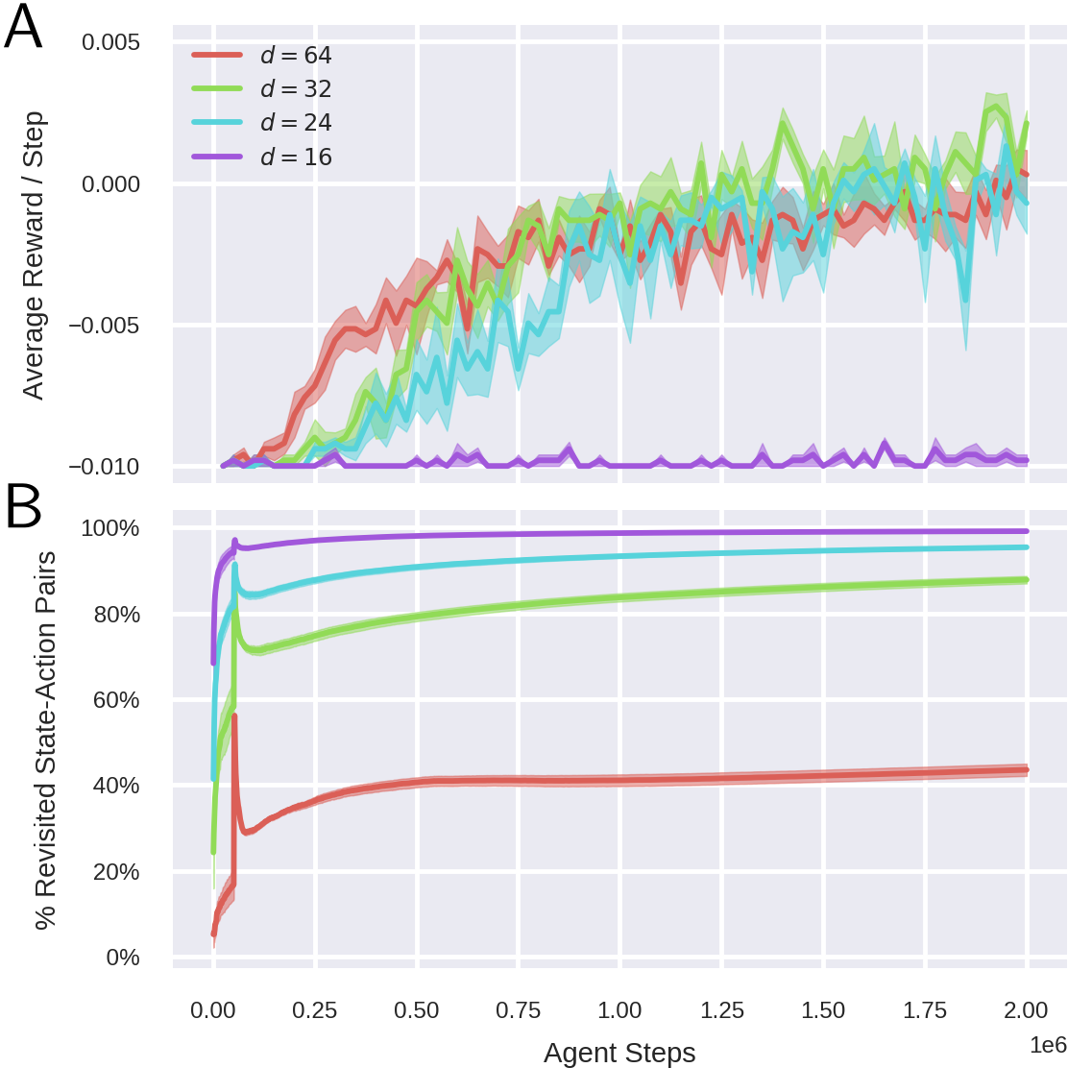
We used latent dimensions for the VaST agent in the navigation tasks, corresponding to a 32–bit representation of the environment. We examine the effect of in Figure 4 and Supplementary Figure 1. High–dimensional representations () tended to plateau at lower performance than representations with , but also resulted in faster initial learning in the more complex maze. The agent frequently revisited state–action pairs even using the high dimensional representation (Figure 4B). In general, we found that we could achieve similar performance with a wide range of dimensionalities; smaller mazes could be learned with as few as 8–16 bits (Supplementary Figure 1).
3.2 Sample efficiency
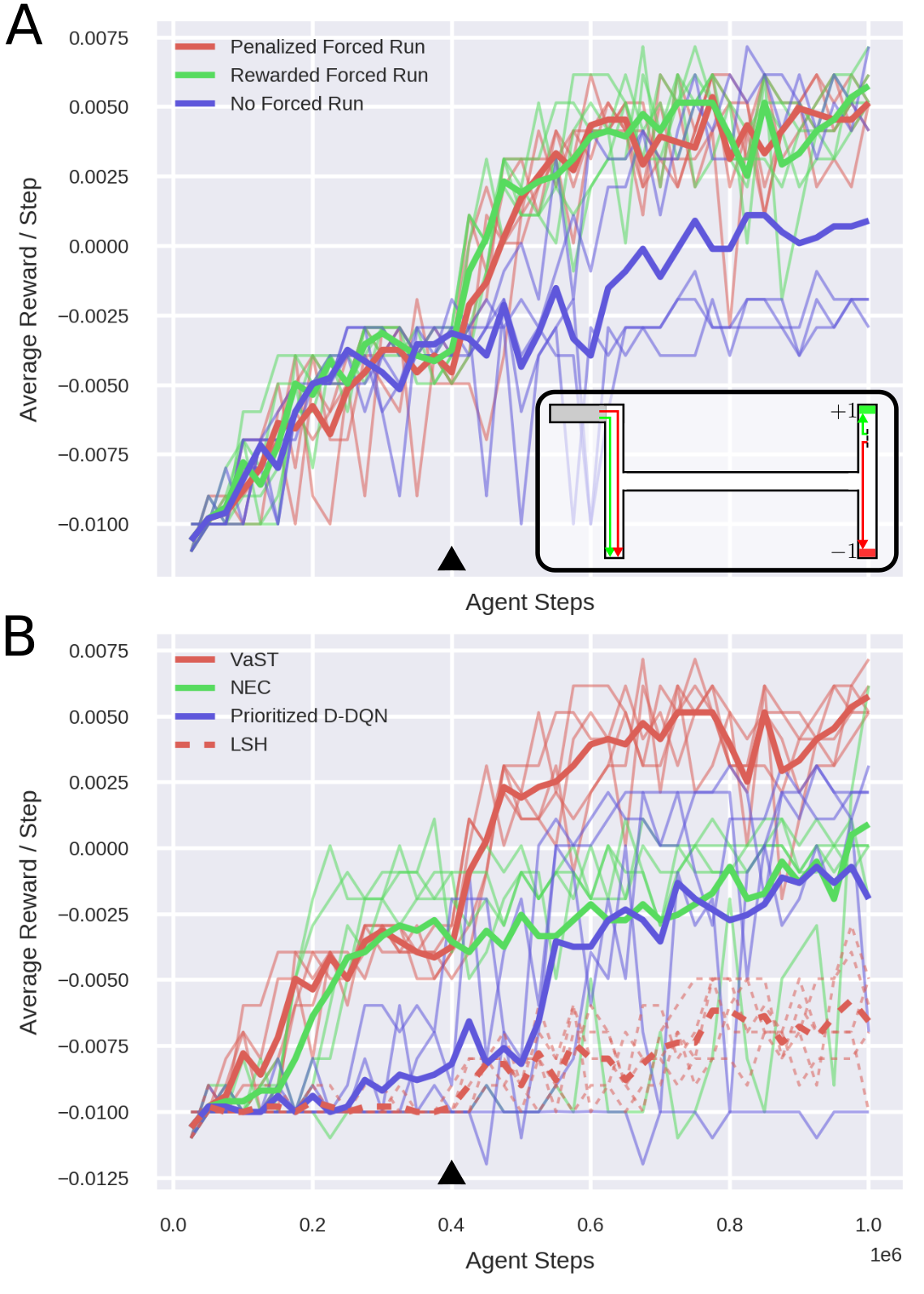
We hypothesized that the VaST agent would be particularly adept at rapidly modifying its policy in response to one new experience. To test this, we designed an experiment in a 3D H–maze (Figure 5) that requires the agent to leverage a single experience of a new shortcut. The agent learned to run towards a terminal reward zone (+1) while avoiding a dead end and a terminal penalty zone (-1), with a step penalty of -0.01. After 400 000 steps of training (when the policy had nearly converged) we introduced a small change to the environment: running into the dead end would cause the agent to teleport to a position close to the reward zone, allowing it to reach the reward much faster. We informed the agent of the teleporter using a single forced run episode, in which the agent collected observations while running from the start box, through the teleporter, to either the reward zone or penalty zone under a fixed, predetermined policy. For the VaST agent, this corresponds to a single experience indicating a new shortcut: the transition between the states before and after the teleporter. After observing either the rewarded or penalized episode, performance rapidly improved as the agent adapted its policy to using the teleporter; in contrast, the agent discovered the teleporter on only 2/5 random seeds without the forced run. The agents switched to using the teleporter regularly approximately 20 000 steps after the forced run, on average (about 160 episodes). The VaST agent adapted to the teleporter more effectively than any of the other models (Figure 5B and Supplementary Figure 2).
3.3 Transfer learning: non–stationary rewards
VaST keeps separate statistics on immediate rewards and transition probabilities in the environment. If the rewards were suddenly modified, we hypothesized that the existing transition model could allow the agent to rapidly adjust its policy (after collecting enough data to determine that the expected immediate rewards had changed).
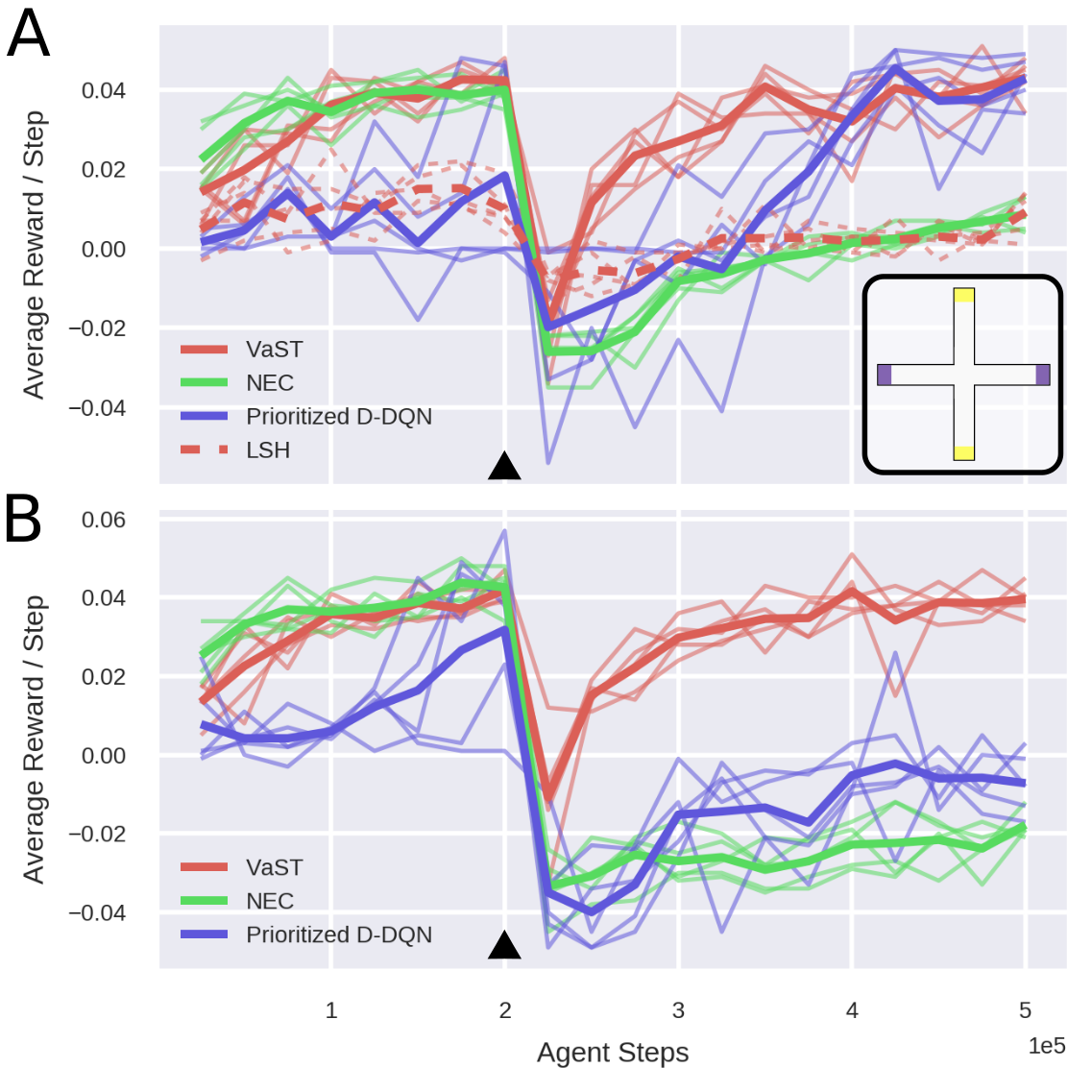
We tested this in the maze shown in Figure 6A (inset). Starting at a random position, the episode terminated at the end of any arm of the maze; the agent received a reward of +1 at the end of horizontal arms, and a penalty of -1 at the end of vertical arms. The reward positions were reversed after 200 000 steps. We used two replay memory sizes ( 100 000 and 500 000). Compared to NEC and Prioritized D–DQN, VaST both learned quickly in the initial phase and recovered quickly when the rewards were reversed. While both NEC and Prioritized D–DQN adapted faster with a smaller replay memory, VaST performed similarly in both conditions.
3.4 Training on Atari: Pong
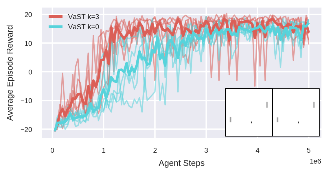
In addition to 3D navigation, we trained the VaST agent to play the Atari game Pong using the Arcade Learning Environment (Bellemare et al., 2013), with preprocessing steps taken from Mnih et al. (2013). In Pong, a table tennis–like game played against the computer, the direction of the ball’s movement is typically unclear given only the current frame as input. We therefore tried conditioning the posterior distribution on either the current frame () or the current frame along with the last 3 frames of input (, following Mnih et al. (2013)). Using , the performance converged significantly faster on average (Figure 7). While the reconstruction cost was the same for and , the transition and entropy cost terms decreased with additional frame history (Supplementary Figure 3).
4 Related Work
Model-based reinforcement learning
Prioritized sweeping with small backups (Van Seijen & Sutton, 2013) is usually more efficient but similar to Dyna-Q (Sutton & Barto, 2018), where a model is learned and leveraged to update Q-values. Prioritized sweeping and Dyna-Q are background planning methods (Sutton & Barto, 2018), in that the action selection policy depends on Q-values that are updated in the background. In contrast, methods that rely on planning at decision time (like Monte Carlo Tree Search) estimate Q-values by expanding the decision tree from the current state up to a certain depth and using the values of the leaf nodes. Both background and decision time planning methods for model-based reinforcement learning are well studied in tabular environments (Sutton & Barto, 2018). Together with function approximation, usually used to deal with high–dimensional raw (pixel) input, many recent works have focused on planning at decision time. Oh et al. (2017) and Farquhar et al. (2017), extending the predictron (Silver et al., 2017), train both an encoder neural network and an action-dependent transition network on the abstract states used to run rollouts up to a certain depth. Racanière et al. (2017) and Nagabandi et al. (2017) train a transition network on the observations directly. Racanière et al. (2017) additionally train a rollout policy, the rollout encoding and an output policy that aggregates different rollouts and a model-free policy. Planning at decision time is advantageous in situations like playing board games (Silver et al., 2017), where the transition model is perfectly known, many states are visited only once and a full tabulation puts high demands on memory. Conversely, background planning has the advantage of little computational cost at decision time, almost no planning cost in well–explored stationary environments and efficient policy updates after minor environment changes.
Successor representations for transfer learning
The hybrid model–based/model–free approach of successor representations has recently been transferred from the tabular domain to deep function approximation (Dayan, 1993; Kulkarni et al., 2016). Under this approach, the agent learns a model of the immediate reward from each state and a model of the expected multi–step future occupancy of each successor state under the current policy. As in a model–based approach, the immediate rewards can be updated independently of the environment dynamics. However, the expected multi–step future occupancy is learned under a given policy, and the optimal policy will generally change with new rewards. The ability to generalize between tasks in an environment (as VaST does in Figure 6) then depends on the similarity between the existing and new policy. Recent work has proposed updating successor representations offline in a Dyna–like fashion using a transition model (Russek et al., 2017; Peng & Williams, 1993); we expect that prioritized sweeping with small backups could also be adapted to efficiently update tabular successor representations.
Navigation tasks
State aggregation in reinforcement learning
State aggregation has a long history in reinforcement learning (Li et al., 2006; Sutton & Barto, 2018). To our knowledge, VaST is the first approach that uses modern deep learning methods to learn useful and non-linear state discretisation. In earlier versions of our model we tried discretising with VAEs as used by (Blundell et al., 2016), with mixed success. The state aggregator of VaST can be seen as a byproduct of training a hybrid ANN–HMM. Different methods to train ANN-HMMs have been studied (Bengio et al., 1992; Tucker et al., 2017; Ng et al., 2016; Maddison et al., 2016). While none of these works study the binary representation of the latent states used by VaST for the generalization of -values, we believe it is worthwhile to explore other training procedures and potentially draw inspiration from the ANN-HMM literature.
5 Discussion
We found that the VaST agent could rapidly transform its policy based on limited new information and generalize between tasks in the same environment. In stationary problems, VaST performed better than competing models in complex 3D tasks where shortcut discovery played a significant role. Notably, VaST performs latent learning; it builds a model of the structure of the environment even when not experiencing rewards (Tolman & Honzik, 1930).
We also trained VaST to play the Atari game Pong. In general, we had less initial success training the agent on other Atari games. We suspect that many Atari games resemble deterministic tree Markov Decision Processes, where each state has exactly one predecessor state. In these tasks, prioritized sweeping conveys no benefit beyond MFEC (Brea, 2017). In contrast, intrinsically continuous tasks like 3D navigation can be well–characterized by a non–treelike tabular representation (e.g. by using a discretisation of (,,), where denotes the agent’s orientation).
VaST differs from many deep reinforcement learning models in that the neural network is entirely reward–agnostic, where training corresponds to an unsupervised learning task. Many other possible architectures exist for the unsupervised tabulator; for instance, a Score Function Estimator such as NVIL (Mnih & Gregor, 2014; Mnih & Rezende, 2016; Tucker et al., 2017) could be used in place of the Con–crete relaxation for discrete stochastic sampling. In addition, while we chose here to show the strengths of a purely model–based approach, one could also consider alternative models that use value information for tabulation, resulting in hybrid model–based/model–free architectures.
The past decade has seen considerable efforts towards using deep networks to adapt tabular RL techniques to high–dimensional and continuous environments. Here, we show how the opposite approach – using deep networks to instead transform the environment into a tabular one – can enable the use of powerful model–based techniques.
Acknowledgements
We thank Vasiliki Liakoni and Marco Lehmann for their invaluable suggestions, feedback and corrections on the manuscript. This work was supported by the Swiss National Science Foundation (grant agreement no. 200020_165538).
References
- Bellemare et al. (2013) Bellemare, M. G., Naddaf, Y., Veness, J., and Bowling, M. The Arcade Learning Environment: An evaluation platform for general agents. Journal of Artificial Intelligence Research, 47:253–279, Jun 2013.
- Bengio et al. (1992) Bengio, Y., De Mori, R., Flammia, G., and Kompe, R. Global optimization of a neural network-hidden markov model hybrid. IEEE Transactions on Neural Networks, 3(2):252–259, Mar 1992. ISSN 1045-9227. doi: 10.1109/72.125866.
- Blundell et al. (2016) Blundell, C., Uria, B., Pritzel, A., Li, Y., Ruderman, A., Leibo, J. Z., Rae, J., Wierstra, D., and Hassabis, D. Model-free episodic control. arXiv preprint arXiv:1606.04460, 2016.
- Brea (2017) Brea, J. Is prioritized sweeping the better episodic control? ArXiv e-prints arXiv:1711.06677, 2017.
- Charikar (2002) Charikar, M. S. Similarity estimation techniques from rounding algorithms. In Proceedings of the thiry-fourth annual ACM symposium on Theory of computing, pp. 380–388. ACM, 2002.
- Dayan (1993) Dayan, P. Improving generalization for temporal difference learning: The successor representation. Neural Computation, 5(4):613–624, 1993.
- Farquhar et al. (2017) Farquhar, G., Rocktäschel, T., Igl, M., and Whiteson, S. TreeQN and ATreeC: Differentiable Tree Planning for Deep Reinforcement Learning. ArXiv e-prints, October 2017.
- Goodfellow et al. (2014) Goodfellow, I., Pouget-Abadie, J., Mirza, M., Xu, B., Warde-Farley, D., Ozair, S., Courville, A., and Bengio, Y. Generative adversarial nets. In Advances in neural information processing systems, pp. 2672–2680, 2014.
- Jaderberg et al. (2016) Jaderberg, M., Mnih, V., Czarnecki, W. M., Schaul, T., Leibo, J. Z., Silver, D., and Kavukcuoglu, K. Reinforcement learning with unsupervised auxiliary tasks. arXiv preprint arXiv:1611.05397, 2016.
- Jang et al. (2016) Jang, E., Gu, S., and Poole, B. Categorical reparameterization with gumbel-softmax. arXiv preprint arXiv:1611.01144, 2016.
- Kempka et al. (2016) Kempka, M., Wydmuch, M., Runc, G., Toczek, J., and Jaśkowski, W. ViZDoom: A Doom-based AI research platform for visual reinforcement learning. In IEEE Conference on Computational Intelligence and Games, pp. 341–348, Santorini, Greece, Sep 2016. IEEE.
- Kingma & Welling (2013) Kingma, D. P. and Welling, M. Auto-encoding variational bayes. arXiv preprint arXiv:1312.6114, 2013.
- Krizhevsky et al. (2012) Krizhevsky, A., Sutskever, I., and Hinton, G. E. Imagenet classification with deep convolutional neural networks. In Advances in neural information processing systems, pp. 1097–1105, 2012.
- Kulkarni et al. (2016) Kulkarni, T. D., Saeedi, A., Gautam, S., and Gershman, S. J. Deep successor reinforcement learning. arXiv preprint arXiv:1606.02396, 2016.
- Li et al. (2006) Li, L., Walsh, T. J., and Littman, M. L. Towards a unified theory of state abstraction for MDPs. In ISAIM, 2006.
- Maddison et al. (2016) Maddison, C. J., Mnih, A., and Whye Teh, Y. The Concrete Distribution: A Continuous Relaxation of Discrete Random Variables. ArXiv e-prints arXiv:1611.00712, November 2016.
- Mirowski et al. (2016) Mirowski, P., Pascanu, R., Viola, F., Soyer, H., Ballard, A. J., Banino, A., Denil, M., Goroshin, R., Sifre, L., Kavukcuoglu, K., Kumaran, D., and Hadsell, R. Learning to Navigate in Complex Environments. ArXiv e-prints, November 2016.
- Mnih & Gregor (2014) Mnih, A. and Gregor, K. Neural variational inference and learning in belief networks. In Xing, E. P. and Jebara, T. (eds.), Proceedings of the 31st International Conference on Machine Learning, volume 32 of Proceedings of Machine Learning Research, pp. 1791–1799, Bejing, China, 22–24 Jun 2014. PMLR.
- Mnih & Rezende (2016) Mnih, A. and Rezende, D. Variational inference for monte carlo objectives. In Proceedings of The 33rd International Conference on Machine Learning, volume 48 of Proceedings of Machine Learning Research, pp. 2188–2196, New York, New York, USA, 20–22 Jun 2016. PMLR.
- Mnih et al. (2013) Mnih, V., Kavukcuoglu, K., Silver, D., Graves, A., Antonoglou, I., Wierstra, D., and Riedmiller, M. Playing atari with deep reinforcement learning. arXiv preprint arXiv:1312.5602, 2013.
- Mnih et al. (2015) Mnih, V., Kavukcuoglu, K., Silver, D., Rusu, A. A., Veness, J., Bellemare, M. G., Graves, A., Riedmiller, M., Fidjeland, A. K., Ostrovski, G., et al. Human-level control through deep reinforcement learning. Nature, 518(7540), 2015.
- Mnih et al. (2016) Mnih, V., Badia, A. P., Mirza, M., Graves, A., Lillicrap, T., Harley, T., Silver, D., and Kavukcuoglu, K. Asynchronous methods for deep reinforcement learning. In International Conference on Machine Learning, pp. 1928–1937, 2016.
- Moore & Atkeson (1993) Moore, A. W. and Atkeson, C. G. Prioritized sweeping: Reinforcement learning with less data and less time. Machine learning, 13(1):103–130, 1993.
- Nagabandi et al. (2017) Nagabandi, A., Kahn, G., Fearing, R. S., and Levine, S. Neural Network Dynamics for Model-Based Deep Reinforcement Learning with Model-Free Fine-Tuning. ArXiv e-prints, August 2017.
- Ng et al. (2016) Ng, Y. C., Chilinski, P. M., and Silva, R. Scaling factorial hidden markov models: Stochastic variational inference without messages. In Advances in Neural Information Processing Systems 29, pp. 4044–4052. 2016.
- Oh et al. (2017) Oh, J., Singh, S., and Lee, H. Value prediction network. In Advances in Neural Information Processing Systems, pp. 6120–6130, 2017.
- Peng & Williams (1993) Peng, J. and Williams, R. J. Efficient learning and planning within the dyna framework. Adaptive Behavior, 1(4):437–454, 1993.
- Pritzel et al. (2017) Pritzel, A., Uria, B., Srinivasan, S., Badia, A. P., Vinyals, O., Hassabis, D., Wierstra, D., and Blundell, C. Neural episodic control. In Proceedings of the 34th International Conference on Machine Learning, volume 70, 2017.
- Racanière et al. (2017) Racanière, S., Weber, T., Reichert, D., Buesing, L., Guez, A., Rezende, D. J., Badia, A. P., Vinyals, O., Heess, N., Li, Y., et al. Imagination-augmented agents for deep reinforcement learning. In Advances in Neural Information Processing Systems, pp. 5694–5705, 2017.
- Rezende et al. (2014) Rezende, D. J., Mohamed, S., and Wierstra, D. Stochastic backpropagation and approximate inference in deep generative models. arXiv preprint arXiv:1401.4082, 2014.
- Riedmiller (2005) Riedmiller, M. Neural fitted q iteration–first experiences with a data efficient neural reinforcement learning method. In European Conference on Machine Learning, pp. 317–328. Springer, 2005.
- Russek et al. (2017) Russek, E. M., Momennejad, I., Botvinick, M. M., Gershman, S. J., and Daw, N. D. Predictive representations can link model-based reinforcement learning to model-free mechanisms. PLOS Computational Biology, 13(9):e1005768, 2017.
- Schaul et al. (2015) Schaul, T., Quan, J., Antonoglou, I., and Silver, D. Prioritized experience replay. arXiv preprint arXiv:1511.05952, 2015.
- Silver et al. (2017) Silver, D., Hubert, T., Schrittwieser, J., Antonoglou, I., Lai, M., Guez, A., Lanctot, M., Sifre, L., Kumaran, D., Graepel, T., Lillicrap, T., Simonyan, K., and Hassabis, D. Mastering Chess and Shogi by Self-Play with a General Reinforcement Learning Algorithm. ArXiv e-prints, December 2017.
- Silver et al. (2017) Silver, D., van Hasselt, H., Hessel, M., Schaul, T., Guez, A., Harley, T., Dulac-Arnold, G., Reichert, D., Rabinowitz, N., Barreto, A., and Degris, T. The predictron: End-to-end learning and planning. In Proceedings of the 34th International Conference on Machine Learning, volume 70, 2017.
- Sutton & Barto (2018) Sutton, R. S. and Barto, A. G. Reinforcement Learning: An Introduction. MIT Press, Cambridge, MA, (in progress) second edition, 2018. URL http://incompleteideas.net/book/the-book-2nd.html.
- Tolman & Honzik (1930) Tolman, E. C. and Honzik, C. H. Introduction and removal of reward, and maze performance in rats. University of California publications in psychology, 1930.
- Tucker et al. (2017) Tucker, G., Mnih, A., Maddison, C. J., Lawson, D., and Sohl-Dickstein, J. REBAR: Low-variance, unbiased gradient estimates for discrete latent variable models. ArXiv e-prints, March 2017.
- Van Seijen & Sutton (2013) Van Seijen, H. and Sutton, R. S. Efficient planning in MDPs by small backups. In Proceedings of the 30th International Conference on Machine Learning, volume 28, 2013.