Quantum Spectral Curve and Structure Constants in $\mathcal{N}=4$ SYM: Cusps in the Ladder Limit

Abstract

We find a massive simplification in the non-perturbative expression for the structure constant of Wilson lines with $3$ cusps when expressed in terms of the key Quantum Spectral Curve quantities, namely Q-functions. Our calculation is done for the configuration of $3$ cusps lying in the same plane with arbitrary angles in the ladders limit. This provides strong evidence that the Quantum Spectral Curve is not only a highly efficient tool for finding the anomalous dimensions but also encodes correlation functions with all wrapping corrections taken into account to all orders in the ‘t Hooft coupling. We also show how to study the insertions of scalars coupled to the Wilson lines and extend our results for the spectrum and the structure constants to this case. We discuss an OPE expansion of two cusps in terms of these states. Our results give additional support to the Separation of Variables strategy in solving the planar ${\cal N}=4$ SYM theory.

1 Introduction

Integrability is a unique tool allowing one to obtain exact non-perturbative results in fully interacting field theories even when the supersymmetry is of no use. The range of theories where integrability is known to be applicable includes supersymmetric theories such as planar ${\cal N}=4$ SYM and ABJM theory, which are important from a holographic perspective. Quite significantly, recently found examples of integrable theories include a particular class of scalar models in 4D possessing no supersymmetry at all Gurdogan:2015csr ; Caetano:2016ydc ; Gromov:2017cja ; Grabner:2017pgm ; Kazakov:2018qbr .

Integrability methods of the type used here started being developed in the seminal papers bfklint in the QCD context and independently in Minahan:2002ve for ${\cal N}=4$ SYM. After almost $20$ years of development it was shown that both approaches can be united by the Quantum Spectral Curve (QSC) formalism Gromov:2013pga ; Gromov:2014caa of which both are some particular limits Gromov:2014caa ; Alfimov:2014bwa .

The QSC was initially developed with the primary goal of computing the spectrum of anomalous dimensions or, equivalently, two point correlators. The QSC is based on the Q-system, a system of functional equations on Q-functions (see Gromov:2017blm ; Kazakov:2018ugh for a recent review). At the same time, the Q-functions are known to play the role of the wave functions in the Separation of Variables (SoV) program initiated for quantum integrable models in Sklyanin:1989cg ; Sklyanin:1991ss ; Sklyanin:1992eu ; Sklyanin:1995bm and recently generalized to $SU(N)$ spin chains in Gromov:2016itr leading to a new algebraic construction for the states (see also Smirnov2001 ; Chervov:2007bb ). In all these models the Q-functions (Baxter polynomials in this case) give the wave functions in separated variables . From this perspective it is natural to expect that the Q-functions of the QSC construction in ${\cal N}=4$ SYM contain much more information than the spectrum and should also play an important role for more general observables.

There are a few important lessons one can learn from the simple spin chains. In particular one should introduce “twists” (quasi-periodic boundary conditions/external magnetic field) in order for the SoV construction to work nicely. One of the main reasons why the twists are important is that they break global symmetry and remove degeneracy in the spectrum. This makes the map between the Q-functions and the states bijective. Fortunately, one can rather easily introduce twists into the QSC construction Gromov:2013qga ; Gromov:2015dfa ; Kazakov:2015efa (see also Klabbers:2017vtw ), however the interpretation of these new parameters is not always clear from the QFT point of view. The $\gamma$-deformation of $\mathcal{N}=4$ SYM Frolov:2005dj ; Alday:2005ww ; Frolov:2005iq ; Beisert:2005if is one of the cases which is rather well understood, but only breaks the R-symmetry part (dual to the isometries of $S^{5}$ part of AdS/CFT) of the whole ${\rm PSU}(2,2|4)$ group.

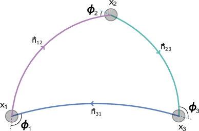
Figure 1: The Maldacena-Wilson loop with three cusps. The cusps are connected by circular arcs with $3$ different scalars $\vec{\Phi}\cdot\vec{n}_{ij}$ coupled to the three different arcs. The expectation value of this object behaves exactly in the same way as a three point correlation function of 3 local operators but provides additional $6$ parameters ($2$ for each cusp) $\phi_{1},\;\phi_{2},\;\phi_{3}$ and $\cos\theta_{1}=\vec{n}_{12}\cdot\vec{n}_{23},\;\cos\theta_{2}=\vec{n}_{23}\cdot\vec{n}_{31},\;\cos\theta_{3}=\vec{n}_{31}\cdot\vec{n}_{12}$, which are associated with twists in the QSC description.

The situation where the twist in both $AdS_{5}$ and $S^{5}$ appears naturally is the cusped Maldacena-Wilson loop. In this paper we consider the correlation function of $3$ cusps for $3$ general angles (see Fig. 1). We consider a ladders limit Erickson:1999qv ; Erickson:2000af where the calculation can be done to all loop orders starting from Feynman graphs. We observe that the result obtained as a resummation of the perturbation theory takes a stunningly simple form when expressed in terms of the Q-functions, which we produced from the QSC.

Set-up and the Main Results.

The Maldacena-Wilson lines we consider are defined as

$$W={\rm Pexp}\int\,d\tau\left(iA_{\mu}\dot{x}^{\mu}+\Phi^{a}n^{a}|\dot{x}|\right),$$ (1.1)

where $n^{a}$ is a constant unit 6-vector parameterizing the coupling to the scalars $\Phi^{a}$ of $\mathcal{N}=4$ SYM. The observable we study is the Wilson loop defined on a planar triangle made of three circular arcs, see Fig. 1. It is parameterized by three cusp angles $\phi_{i}$ at its vertices and also three angles $\theta_{i}$ between the couplings to scalars on the lines adjacent to each vertex. At each cusp we have a divergence controlled by the celebrated cusp anomalous dimension $\Gamma_{\rm cusp}(\phi_{i},\theta_{i})$ which can be efficiently studied via integrability Correa:2012hh ; Drukker:2012de ; Gromov:2015dfa and is analogous to the local operator scaling dimensions in its mathematical description by the QSC. Due to this we will use notation $\Delta$ for the cusp dimension. To regularize the divergence we cut an $\epsilon$-ball at each of the cusps. The whole Wilson loop has a conformally covariant dependence on the cusp positions and defines the structure constant $C_{123}$ for a 3-point correlator of three cusps.

We focus on the ladders limit in which $\theta_{i}\to i\infty$ while the ’t Hooft coupling $g=\sqrt{\lambda}/({4\pi})$ goes to zero with the finite combinations

$$\hat{g}_{i}=\frac{g}{2}e^{-i\theta_{i}/2}$$ (1.2)

playing the role of three effective couplings. The perturbative expansion for $\Delta$ can then be resummed to all orders leading to a stationary Schrödinger equation Erickson:1999qv ; Erickson:2000af ; Correa:2012nk . However, the 3-cusp correlator is much more nontrivial and depends on three couplings $\hat{\lambda}_{i}$ which we can vary separately. We have studied the case when two of them are nonzero, corresponding to the structure constant we denote by $C^{\bullet\bullet\circ}_{123}$. The result may be written in terms of the Schrödinger wave-functions but it is a highly complicated integral which does not offer much structure. Yet once we rewrite it in terms of the QSC Q-functions $q(u)$, we observe miraculous cancellations leading to a surprisingly simple expression

$$\boxed{C^{\bullet\bullet\circ}_{123}=\,\frac{\,{\langle\!\!\langle}q_{1}\,q_{2}\,e^{-\phi_{3}u}{\rangle\!\!\rangle}}{\sqrt{{\langle\!\!\langle}q_{1}^{2}{\rangle\!\!\rangle}{\langle\!\!\langle}q_{2}^{2}{\rangle\!\!\rangle}}}\ \ ,}$$ (1.3)

where the bracket ${\langle\!\!\langle}f(u){\rangle\!\!\rangle}$ is defined for the functions which behave as $\sim e^{u\beta}u^{\alpha}$ at large $u$ and are analytic for all ${\rm Re}\;u>0$ as

$${\langle\!\!\langle}f(u){\rangle\!\!\rangle}\equiv\left(2\sin\frac{\beta}{2}\right)^{\alpha}\int_{c-i\infty}^{c+i\infty}f(u)\frac{du}{2\pi iu}\;\;,\;\;c>0\;.$$ (1.4)

The functions $q_{1}(u),q_{2}(u)$ describe the first and the second cusp, while $e^{-\phi_{3}u}$ is just the Q-function at zero coupling corresponding to the third cusp. Each of the Q-functions solves a simple finite difference equation (2.7). This is precisely the kind of result one expects for an integrable model treated in separated variables. Note that all the dependence on the angles and the couplings is coming solely through the Q-functions, which depend nontrivially on these parameters, in particular at large $u$ we have $q_{i}(u)\simeq u^{\Delta_{i}}e^{\phi_{i}u}$.

We also found a very simple expression for the derivative of $\Delta$ w.r.t. the coupling $\hat{g}$ and the angle $\phi$ in terms of the bracket ${\langle\!\!\langle}\cdot{\rangle\!\!\rangle}$

$$-\frac{1}{4}\frac{\partial\Delta}{\partial\hat{g}^{2}}=\frac{{\langle\!\!\langle}q^{2}\frac{1}{u}{\rangle\!\!\rangle}}{{\langle\!\!\langle}q^{2}{\rangle\!\!\rangle}}\;\;,\;\;-2\,\frac{\partial(\sin\phi\Delta)}{\partial\phi}=\frac{{\langle\!\!\langle}q^{2}u{\rangle\!\!\rangle}}{{\langle\!\!\langle}q^{2}{\rangle\!\!\rangle}}\;,$$ (1.5)

which has the form very similar to (1.3) with $q_{1}=q_{2}=q$ and different insertions in the numerator! These quantites can be interpreted as structure constants of two cusps with a local BPS operator Costa:2010rz .

In the limit when the triangle collapses to a straight line, this configuration has recently attracted much attention as it defines a 1d CFT on the line Giombi:2017cqn ; Beccaria:2017rbe ; Kim:2017sju ; Cooke:2017qgm ; Kim:2017phs . In particular the structure constants we consider were computed in Kim:2017sju by resumming the diagrams using the exact solvability of the Schrödinger problem at $\phi=0$. Our results in the zero angle limit can be simplified further by noticing that for $\phi_{i}\to 0$ the integral is saturated by the leading large $u$ asymptotics of the integrand. This leads to ${\langle\!\!\langle}q_{i}q_{j}{\rangle\!\!\rangle}\to{1/\Gamma(1-\Delta_{i}-\Delta_{j})}$, reproducing the results of Kim:2017sju .

As a byproduct, we also resolved the question of how to use integrability to compute the anomalous dimension for the cusp with an insertion of the same scalar as that coupled to the Wilson lines. We propose that it simply corresponds to one of the excited states in the Schrödinger equation (and to a well-defined analytic continuation in the QSC outside the ladders limit). We verified this claim at weak coupling by comparing with the direct perturbation theory calculation of Alday:2007he . Very recently the importance of the cusps with such insertions were further motivated in Bruser:2018jnc where the $3$ loop result was extracted.

We demonstrate some of our results in Fig. 2 where we show the plots of the spectrum and the structure constant for a range of the effective coupling $\hat{g}$.

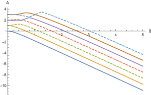
Figure 2: The spectrum (left) and the diagonal Heavy-Heavy-Light correlator given by (1.3) (right) for the first several states ($n=0,1,\dots,7$), with all angles equal to $\phi=1$. The solid blue line corresponds to the usual cusp, while others correspond to excited states with scalar insertions discussed in section 5.

Structure of the paper.

The rest of the paper is organized as follows. In Sec. 2 we briefly review the QSC and present the Baxter equation to which it reduces in the ladders limit. We also derive compact formulas for the variation of $\Delta$ with respect to the coupling and the angle $\phi$. In Sec. 3 we write the regularized 2-pt function in terms of the Schrödinger equation wave functions, in particular deriving the pre-exponent normalization which is important for 3-pt correlators. We also relate the wave functions to the QSC Q-functions via a Mellin transform. In Sec. 4 we study the 3-cusp correlator and derive our main result for the structure constant (1.3). In Sec. 5 we describe the interpretation of excited states in the Schrödinger problem as insertions at the cusp. We generalize our results for 3-pt functions to the excited states and provide both perturbative and numerical data for their scaling dimensions. In Sec. 6 we describe the limit when the 3-cusp configuration degenerates, in particular reproducing the results of Kim:2017sju when all angles become zero. In Sec. 7 and 8 we present numerical and perturbative results for the structure constants. Finally in Sec. 9 we interpret the regularized 2-pt function as a 4-cusp correlator for which we write an OPE-type expansion in terms of the structure constants, perfectly matching our previous results. In Sec. 10 we present conclusions. The appendices contain various technical details, in particular the detailed strong coupling expansion for the spectrum.

2 Quantum Spectral Curve in the ladders limit

In this section we provide all necessary background for this paper about the Quantum Spectral Curve (QSC). More technical details are given in Appendix A.

The QSC provides a finite set of equations describing non-perturbatively the cusp anomalous dimension $\Delta$ at all values of the parameters $\phi,\theta$ and any coupling $g$. Let us briefly review this construction and then discuss the form it takes in the ladders limit. The QSC was originally developed in Gromov:2013pga ; Gromov:2014caa for the spectral problem of local operators in $\mathcal{N}=4$ SYM. It was extended in Gromov:2015dfa to describe the cusp anomalous dimension, reformulating and greatly simplifying the TBA approach of Correa:2012hh ; Drukker:2012de . The QSC is a set of difference equations (QQ-relations) for the Q-functions which are central objects in the integrability framework. When supplemented with extra asymptotics and analyticity conditions, these relations fix the Q-functions and provide the exact anomalous dimension $\Delta$ (see Gromov:2017blm for a pedagogical introduction and Kazakov:2018ugh for a wider overview).

The QSC is based on 4+4 basic Q-functions denoted as ${\bf P}_{a}(u)$, $a=1,\dots,4$ and ${\bf Q}_{i}(u)$, $i=1,\dots,4$ which are related to the dynamics on $S^{5}$ and on $AdS_{5}$ correspondingly. The ${\bf P}$-functions are analytic functions of $u$ except for a cut at $[-2g,2g]$. They can be nicely parameterized in terms of an infinite set of coefficients that contain full information about the state, including $\Delta$. Details of this parameterization are given in Appendix A. The other 4 basic Q-functions ${\bf Q}_{i}$ are indirectly determined by ${\bf P}_{a}$ via the 4th order Baxter equation Alfimov:2014bwa

$${\bf Q}^{[+4]}_{i}D_{0} - {\bf Q}^{[+2]}\left[D_{1}-{\bf P}_{a}^{[+2]}{\bf P}^{a[+4]}D_{0}\right]+{\bf Q}\left[D_{2}-{\bf P}_{a}{\bf P}^{a[+2]}D_{1}+{\bf P}_{a}{\bf P}^{a[+4]}D_{0}\right]$$

$$- {\bf Q}^{[-2]}\left[\bar{D}_{1}+{\bf P}_{a}^{[-2]}{\bf P}^{a[-4]}\bar{D}_{0}\right]+{\bf Q}^{[-4]}\bar{D}_{0}=0\ ,$$

where the coefficients $D_{n},\bar{D}_{n}$ are simple determinants built from ${\bf P}_{a}$ and are given explicitly in Appendix A. Here we used the shorthand notation

$$f^{\pm}=f(u\pm\tfrac{i}{2}),\ \ f^{[+a]}=f(u+\tfrac{ia}{2})\ .$$ (2.2)

Being of the 4th order, this Baxter equation has four independent solutions which precisely correspond to the four Q-functions ${\bf Q}_{i}$. Different solutions can be identified by the four possible asymptotics ${\bf Q}_{i}\sim u^{1/2\pm\Delta}e^{\pm u\phi}$ which uniquely fix the basis of four Q-functions up to a normalization if we also impose that the solutions ${\bf Q}_{i}(u)$ are analytic in the upper half-plane of $u$, which is always possible to do. Then they will have an infinite set of Zhukovsky cuts in the lower half-plane with branch points at $u=\pm 2g-in$ (with $n=0,1,\dots$).

Finally in order to close the system of equations we need to impose what happens after the analytic continuation through the cut $[-2g,2g]$. It was shown in Gromov:2015dfa that in order to close the equations one should impose the following “gluing” conditions

$$\tilde{q}_{1}(u)={q}_{1}(-u)$$ (2.3)

$$\tilde{q}_{2}(u)={q}_{2}(-u)$$ (2.4)

$$\tilde{q}_{3}(u)=a_{1}\sinh(2\pi u){q}_{2}(-u)+{q}_{3}(-u)$$ (2.5)

$$\tilde{q}_{4}(u)=a_{2}\sinh(2\pi u){q}_{1}(-u)+{q}_{4}(-u)\;,$$ (2.6)

where $q_{i}(u)={\bf Q}_{i}(u)/\sqrt{u}$ and $\tilde{q}_{i}$ is its analytic continuation under the cut. These relations fix both ${\bf P}$- and ${\bf Q}$-functions and allow one to extract the exact cusp anomalous dimension $\Delta$ from large $u$ asymptotics. The equations presented above are valid at any values of $g$ and the angles $\phi,\theta$. For the purposes of this paper we have to take the ladders limit of these equations. We will see that they simplify considerably.

2.1 Baxter equation in the ladders limit

In the ladders limit (1.2) the coupling $g$ goes to zero and the QSC greatly simplifies as all the branch cuts of the Q-functions collapse and simply become poles. This limit was explored in detail in Gromov:2016rrp for the special case $\phi=\pi$ corresponding to the flat space quark-antiquark potential. Here we briefly generalize these results to the generic $\phi$ case.

The key simplification is that the 4th order Baxter equation (2) on ${\bf Q}_{i}$ factorizes into two 2nd order equations, the first one being

$$\boxed{\left(-2u^{2}\cos\phi+2\Delta u\sin\phi+4\hat{g}^{2}\right){q}(u)+u^{2}{q}(u-i)+u^{2}{q}(u+i)=0}$$ (2.7)

and another equation obtained by $\Delta\to-\Delta$. This follows from the fact that coefficients $A_{n},B_{n}$ entering ${\bf P}$’s via (A.1), (A.4) scale as $\sim 1$ in the ladders limit. Then as in Gromov:2016rrp one can carefully expand the 4th order Baxter equation for $t\equiv e^{i\theta/2}\to 0$ and recover the 2nd order equation (2.7). As the large $u$ behaviour of $q(u)$ is fixed by the Baxter equation (2.7), we denote them as $q_{+}$ and $q_{-}$ according to the large $u$ asymptotics $q_{\pm}\sim e^{\pm\phi u}u^{\pm\Delta}$. For example in the weak coupling limit $\hat{g}=0$ for $\Delta=0$ we see that $q_{\pm}$ are simply

$$q^{(0)}_{+}=e^{+\phi u}\;\;,\;\;q^{(0)}_{-}=e^{-\phi u}\;.$$ (2.8)

At finite $\hat{g}$ the Q-functions become rather nontrivial. While $q_{\pm}(u)$ are regular in the upper half-plane including the origin, they have poles in the lower half-plane at $u=-in,\ \ n=1,2,\dots$.

The equation (2.7) is just an $sl(2)$ (non-compact) spin chain Baxter equation, similarly to Gromov:2017cja . This is expected based on symmetry grounds. What is less trivial is the “quantization condition” i.e. the condition which will restrict $\Delta$ to a discrete set. It was first derived in Gromov:2016rrp for $\phi\to\pi$ and later generalized to the very similar calculation of two-point functions in the fishnet model Gromov:2017cja . The derivation of the quantization condition for any $\phi$ is done in Appendix A and leads to the following result:

$$\boxed{\Delta=-\frac{2\hat{g}^{2}}{\sin\phi}\frac{q_{+}(0)\bar{q}_{+}^{\prime}(0)+\bar{q}_{+}(0)q_{+}^{\prime}(0)}{q_{+}(0)\bar{q}_{+}(0)}}\;.$$ (2.9)

Together with the Baxter equation (2.7), this relation fixes $\Delta$ as well as $q_{+}$.

Note that the r.h.s.​ of (2.9) contains $q_{+}$, which has to be found from the Baxter equation and thus also depends on $\Delta$ nontrivially. Due to this (2.9) is a non-linear equation, which may have several solutions. Some intuition behind it becomes clearer after reformulating the problem in a more standard Schrödinger equation form as we will see in section 3.1. At the same time we see that we only need $q_{+}$ to find the spectrum. For this reason we will simply denote it as $q(u)$ in the rest of the paper.

The meaning of the Q-functions from the QFT point of view is still a big mystery. There is no known observable in the field theory which is known to correspond to them directly. However in the “fishnet” theory, which is a particular limit of ${\cal N}=4$ SYM, such an object was recently identified Gromov:2017cja . Here, in the ladders limit we will be able to relate $q(u)$ with a solution of the Bethe-Salpeter equation, which resums the ladder Feynman diagrams and thus has direct field theory interpretation.

2.2 Scalar product and variations of $\Delta$

In this section we demonstrate the significance of the bracket ${\langle\!\!\langle}\cdot{\rangle\!\!\rangle}$, which we defined in the introduction in (1.4). In particular we will derive a closed expression for ${\partial\Delta}/{\partial\hat{g}}$ which can be considered as a correlation function of two cusps with the Lagrangian Costa:2010rz . Even though that seems to be the simplest application of the QSC for the computation of the $3$-point correlators, it is not yet known how to write the result for $\partial\Delta/\partial g$ for the general state in a closed form. We demonstrate here that this is in fact possible to do at least in our simplified set-up.

First we rewrite the Baxter equation (2.7) by defining the following finite difference operator

$$\hat{O}\equiv\frac{1}{u}\left[(4\hat{g}^{2}-2u^{2}\cos\phi+2\Delta u\sin\phi)+u(u-i)D^{-1}+u(u+i)D\right]\frac{1}{u}$$ (2.10)

where $D$ is a shift by $i$ operator so that the Baxter equation (2.7) becomes

$$\hat{O}q(u)=0\;.$$ (2.11)

Now we notice that this operator is “self-adjoint” under the integration along the vertical contour to the right from the origin, meaning that

$$\int_{{\bf|}}q_{1}(u)\hat{O}q_{2}(u)du=\int_{{\bf|}}q_{2}(u)\hat{O}q_{1}(u)du\;\;,\;\;\int_{{\bf|}}\equiv\int_{c-i\infty}^{c+i\infty}\ .$$ (2.12)

where $c>0$. Indeed, consider the term with $D$:

$$\int_{{\bf|}}q_{1}(u)u(u+i)Dq_{2}(u)du=\int_{{\bf|}}q_{1}(u)u(u+i)q_{2}(u+i)du=\int_{{\bf|}}q_{2}(u)u(u-i)D^{-1}q_{1}(u)du$$ (2.13)

which now became the term with $D^{-1}$ acting on $q_{1}(u)$. In the last equality we changed the integration variable $u\to u-i$. The fact that $\hat{O}$ has this property immediately leads to the great simplification for the expression for $\partial\Delta/\partial g$. We can now apply the standard QM perturbation theory logic.

Changing the coupling and/or the angle $\phi$ will lead to a perturbation of both the operator $\hat{O}$ and the q-function in such a way that the Baxter equation is still satisfied ,

$$(\hat{O}+\delta\hat{O})(q+\delta q)=0\;\;,\;\;\delta\hat{O}=\frac{1}{u^{2}}(8\hat{g}\delta\hat{g}+2u\sin\phi\delta\Delta+2u^{2}\sin\phi\delta\phi+2\Delta u\cos\phi\delta\phi)\;.$$ (2.14)

An explicit expression for $\delta q$ could be rather hard to find, but luckily we can get rid of it by contracting $(\hat{O}+\delta\hat{O})(q+\delta q)$ with the original $q(u)$:

$$0=\int_{{\bf|}}q(\hat{O}+\delta\hat{O})(q+\delta q)du=\int_{{\bf|}}(q+\delta q)(\hat{O}+\delta\hat{O})qdu=\int_{{\bf|}}(q+\delta q)\delta\hat{O}qdu$$ (2.15)

At the leading order in the perturbation we can now drop $\delta q$ to obtain

$$\int_{{\bf|}}q(8\hat{g}\delta\hat{g}+2u\sin\phi\delta\Delta+2u^{2}\sin\phi\delta\phi+2\Delta u\cos\phi\delta\phi)q\frac{du}{u^{2}}=0\ ,$$ (2.16)

so that

$$\frac{\partial\Delta}{\partial\hat{g}}=-\frac{4\hat{g}}{\sin\phi}\frac{\int_{{\bf|}}\frac{q^{2}}{u^{2}}du}{\int_{{\bf|}}\frac{q^{2}}{u}{du}}\;\;,\;\;\frac{\partial\Delta}{\partial\phi}=-\frac{\int_{{\bf|}}q^{2}du}{\int_{{\bf|}}\frac{q^{2}}{u}{du}}-\Delta\cot\phi\;.$$ (2.17)

In terms of the bracket ${\langle\!\!\langle}\cdot{\rangle\!\!\rangle}$ this becomes

$$\boxed{-\frac{1}{4}\frac{\partial\Delta}{\partial\hat{g}^{2}}=\frac{{\langle\!\!\langle}q^{2}\frac{1}{u}{\rangle\!\!\rangle}}{{\langle\!\!\langle}q^{2}{\rangle\!\!\rangle}}\;\;,\;\;-2\,\frac{\partial(\sin\phi\Delta)}{\partial\phi}=\frac{{\langle\!\!\langle}q^{2}u{\rangle\!\!\rangle}}{{\langle\!\!\langle}q^{2}{\rangle\!\!\rangle}}\;.}$$ (2.18)

This very simple equation is quite powerful. For example by plugging the leading order $q=e^{u\phi}$ from (2.8) and computing the integrals by poles at $u=0$ we get

$$\frac{\partial\Delta}{\partial\hat{g}}=-\frac{4\hat{g}}{\sin\phi}2\phi+{\cal O}(\hat{g}^{3})\;,$$ (2.19)

which gives immediately the one loop dimension $\Delta=-\hat{g}^{2}\frac{4\phi}{\sin\phi}+{\cal O}(\hat{g}^{4})$.

Furthermore, another interesting property of the bracket is that solutions with different $\Delta^{\prime}s$ are orthogonal to each other. Indeed, consider two solutions $q_{a}$ of the Baxter equation with two different dimensions $\Delta_{a}$, such that $\hat{O}_{1}q_{1}=\hat{O}_{2}q_{2}=0$. Then

$$0=\int_{{\bf|}}q_{1}(u)(\hat{O}_{1}-\hat{O}_{2})q_{2}(u)du=(\Delta_{1}-\Delta_{2})2\sin\phi\int_{{\bf|}}\frac{q_{1}(u)q_{2}(u)}{u}du\ ,$$ (2.20)

from which we conclude that ${\langle\!\!\langle}q_{1}(u)q_{2}(u){\rangle\!\!\rangle}=0$.

In the next section we relate the Q-function to the solution of the Bethe-Salpeter equation resumming the ladder diagrams for the two point correlator.

3 Bethe-Salpeter equations and the Q-function

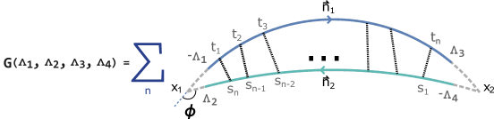
Figure 3: The two cusp correlator with four different cut-offs $\Lambda_{a}$, which can be considered as a particular case of $4$-cusp correlator. We take $n$ points along each of the circular arcs and connect them with scalar propagators. We have to integrate over the domain $-\Lambda_{1}<t_{1}<t_{2}<\dots<t_{n}<\Lambda_{3}$ and $-\Lambda_{4}<s_{1}<s_{2}<\dots s_{n}<\Lambda_{2}$. One should use a specific parameterization given in (3.3).

In this section we consider a two cusp correlator with amputated cusps shown on Fig. 3 which we denote by $G(\Lambda_{1},\Lambda_{2},\Lambda_{3},\Lambda_{4})$. We derive an expression for it re-summing the ladder diagrams. To do this we write a Bethe-Salpeter equation and then reduce it to a stationary Schrödinger equation, expressing $G$ in terms of the wave functions and energies of the Schrödinger problem. After that we discuss the relation between the wave functions and the Q-functions introduced in the previous section.

3.1 Bethe-Salpeter equation

Our goal in this section is reviewing the field-theoretical definition of the cusp anomalous dimension and its computation in the ladder limit, where it relates to the ground state energy of a simple Schrödinger problem.

First we define more rigorously the object from the Fig. 3. We are computing an expectation value

$$G(\Lambda_{1},\Lambda_{2},\Lambda_{3},\Lambda_{4})=\left\langle{\rm Tr\;}W_{\vec{x}_{+}(-\Lambda_{1})}^{\vec{x}_{+}(+\Lambda_{3})}(\vec{n}_{1})\;\;W_{\vec{x}_{-}(-\Lambda_{4})}^{\vec{x}_{-}(+\Lambda_{2})}(\vec{n}_{2})\right\rangle,$$ (3.1)

with

$$W_{x}^{y}(\vec{n})={\rm Pexp}\int_{x}^{y}\left(iA_{\mu}dx^{\mu}+\Phi^{a}n^{a}|dx|\right).$$ (3.2)

For simplicity we can assume that the contours belong to the $(*,*,0,0)$ two dimensional plane (which can be always achieved with a suitable rotation) and we use a particular “conformal” parameterization of the circular arcs by

$$\vec{x}_{\pm}(s)=(\text{Re}(\zeta_{\pm}(s)),\text{Im}(\zeta_{\pm}(s)),0,0),$$ (3.3)

where

$$\zeta_{{}_{\pm}}(s) = z_{1}+\frac{(z_{2}-z_{1})}{1\mp ie^{\mp s+i(\chi\pm\phi)/2}}$$ (3.4)

such that $\vec{x}_{1}\equiv(\text{Re}(z_{1}),\text{Im}(z_{1}),0,0)=\vec{x}_{\pm}(\mp\infty)$ and $\vec{x}_{2}=(\text{Re}(z_{2}),\text{Im}(z_{2}),0,0)=\vec{x}_{\pm}(\pm\infty)$. Here $\vec{x}_{+}$ corresponds to the upper arc in Fig. 3, and $\vec{x}_{-}$ to the lower one. The configuration has one parameter $\chi$, which allows one to bend two arcs simultaneously keeping the angle between them fixed. This is the most general configuration of two intersecting circular arcs up to a rotation.

Next we notice that in the ladders limit we can neglect gauge fields so we get

$$\partial_{\Lambda_{3}}\partial_{\Lambda_{4}}G(\Lambda_{1},\Lambda_{2},\Lambda_{3},\Lambda_{4})=$$ (3.5)

$$\left\langle{\rm Tr}\;W_{\vec{x}_{+}(-\Lambda_{1})}^{\vec{x}_{+}(+\Lambda_{3})}(\vec{n}_{1})\;\;\Phi^{a}n_{1}^{a}|\dot{\vec{x}}_{+}(\Lambda_{3})|\;\;\Phi^{b}n_{2}^{b}|\dot{\vec{x}}_{-}(-\Lambda_{4})|\;\;W_{\vec{x}_{-}(-\Lambda_{4})}^{\vec{x}_{-}(+\Lambda_{2})}(\vec{n}_{2})\right\rangle,$$

which gives

$$\partial_{\Lambda_{3}}\partial_{\Lambda_{4}}G(\Lambda_{1},\Lambda_{2},\Lambda_{3},\Lambda_{4})=G(\Lambda_{1},\Lambda_{2},\Lambda_{3},\Lambda_{4})P(-\Lambda_{4},\Lambda_{3})\ ,$$ (3.6)

where the last term is the scalar propagator

$$P(s,t)=4\,\hat{g}^{2}\,\frac{|\dot{\vec{x}}_{-}(s)|\,|\dot{\vec{x}}_{+}(t)|}{|\vec{x}_{+}(t)-\vec{x}_{-}(s)|^{2}}$$ (3.7)

with $\hat{g}^{2}=g^{2}\vec{n}_{a}\cdot\vec{n}_{b}/2$ (which is equivalent in the ladders limit to the definition of $\hat{g}$ in (1.2) as $\vec{n}_{1}\cdot\vec{n}_{2}=\cos\theta$). The main advantage of the parameterization we used is that the propagator $P(s,t)$ is a function of the sum $s+t$:

$$P(s,t)=\frac{2\hat{g}^{2}}{\cosh(s+t)+\cos(\phi)}\;.$$ (3.8)

Finally, we have to specify the boundary conditions. We notice that whenever one of the Wilson lines degenerates to a point the expectation value in the ladders limit becomes $1$, which implies

$$G(\Lambda_{1},\Lambda_{2},-\Lambda_{1},\Lambda_{4})=G(\Lambda_{1},\Lambda_{2},\Lambda_{3},-\Lambda_{2})=1\;.$$ (3.9)

Stationary Schrödinger equation.

In order to separate the variables we introduce new “light-cone” coordinates in the following way

$$x=\Lambda_{4}-\Lambda_{3}\;\;,\;\;y=\frac{\Lambda_{1}+\Lambda_{2}+\Lambda_{3}+\Lambda_{4}}{2}$$ (3.10)

so that $\partial_{\Lambda_{3}}\partial_{\Lambda_{4}}=-\partial_{x}^{2}+\frac{1}{4}\partial_{y}^{2}$. We also denote

$$\tilde{G}_{\Lambda_{1},\Lambda_{2}}(x,y)\equiv G(\Lambda_{1},\Lambda_{2},\Lambda_{3},\Lambda_{4})$$ (3.11)

so that (3.5) becomes

$$\frac{1}{4}\partial_{y}^{2}\tilde{G}_{\Lambda_{1},\Lambda_{2}}(x,y)=\left[\partial_{x}^{2}+\frac{2\hat{g}^{2}}{\cosh x+\cos\phi}\right]\tilde{G}_{\Lambda_{1},\Lambda_{2}}(x,y)\;.$$ (3.12)

In order to completely reduce this equation to the stationary Schrödinger problem, we have to extend the function $G_{\Lambda_{1},\Lambda_{2}}(x,y)$ to the whole plane. Currently it is only defined for $-\Lambda_{1}<\Lambda_{3}$ and $-\Lambda_{2}<\Lambda_{4}$ i.e. inside the future light-cone, see Fig. 4. We extend $\tilde{G}_{\Lambda_{1},\Lambda_{2}}(x,y)$ to the whole plane using the following definition:

$$\tilde{G}_{\Lambda_{1},\Lambda_{2}}(x,y) = -\tilde{G}_{\Lambda_{1},\Lambda_{2}}(x,|y|)\;\;,\;\;y<0$$ (3.13)

$$\tilde{G}_{\Lambda_{1},\Lambda_{2}}(x,y) = 0\;\;,\;\;|y|>|x-\Lambda_{1}+\Lambda_{2}|/2\;.$$ (3.14)

With this definition it is easy to see that if (3.12) was satisfied in the future light cone, it will hold for the whole plane.

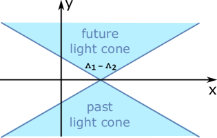
Figure 4: We have to impose the boundary condition $\tilde{G}_{\Lambda_{1},\Lambda_{2}}(x,y)=1$ on the light-rays intersecting at $x=\Lambda_{1}-\Lambda_{2}$ and given by the equation $x=\Lambda_{1}-\Lambda_{2}\pm 2y$. The initial function $\tilde{G}_{\Lambda_{1},\Lambda_{2}}(x,y)$ is only defined inside the future light cone. It can be extended to the whole plane by setting it to zero outside the light cone and imposing $\tilde{G}_{\Lambda_{1},\Lambda_{2}}(x,y)=-\tilde{G}_{\Lambda_{1},\Lambda_{2}}(x,-y)$ for negative $y$.

After that we can expand $\tilde{G}_{\Lambda_{1},\Lambda_{2}}(x,y)$ in the complete basis of the eigenfunctions of the Schrödinger equation in the $x$ direction,

$$\tilde{G}_{\Lambda_{1},\Lambda_{2}}(x,y)=\sum_{n}a_{n}(y)F_{n}(x)$$ (3.15)

where

$$4\left[-\partial_{x}^{2}-\frac{2\hat{g}^{2}}{\cosh x+\cos\phi}\right]F_{n}(x)={E_{n}}F_{n}(x)\;$$ (3.16)

and $a_{n}(y)$ has to satisfy $a_{n}^{\prime\prime}(y)=-E_{n}a_{n}(y)$. Since $\tilde{G}(x,y)$ is odd in $y$ we get

$$\tilde{G}_{\Lambda_{1},\Lambda_{2}}(x,y)=\sum\int_{n}C_{n}(\Lambda_{1},\Lambda_{2})\left(e^{\sqrt{-E_{n}}\,y}-e^{-\sqrt{-E_{n}}\,y}\right)F_{n}(x)\;.$$ (3.17)

In the above expression we assume the sum over all bound states with $E_{n}<0$ and integral over the continuum $E_{n}>0$ (see Fig. 5).

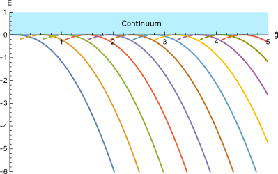
Figure 5: Spectrum of the Schrödinger problem at $\phi=1.5$ for a range of values of the coupling. Solid lines show numerical data for the first few bound states. For small $\hat{g}$ there is only one bound state in the spectrum, but their number grows linearly with the coupling. Dashed lines show analytic continuation of the levels in the coupling $\hat{g}$ beyond the point where they disappear from the bound state spectrum and become resonances (to be discussed in detail in section 5.3).

Next we should determine the coefficients $C_{n}(\Lambda_{1},\Lambda_{2})$, for that we consider the small $y$ limit. For small $y$ we see that $G(x,y)$ is almost constant inside the light cone ($+1$ for $y>0$ and $-1$ for $y<0$) and is zero for $\Lambda_{1}-\Lambda_{2}-2y<x<\Lambda_{1}-\Lambda_{2}+2y$. In other words for small $y$ we have

$$\tilde{G}_{\Lambda_{1},\Lambda_{2}}(x,y)\simeq 4y\delta(x-\Lambda_{1}+\Lambda_{2})$$ (3.18)

at the same time from the ansatz (3.17) we have, in the small $y$ limit

$$\tilde{G}_{\Lambda_{1},\Lambda_{2}}(x,y)\simeq 2y\sum\int_{n}C_{n}(\Lambda_{1},\Lambda_{2})\sqrt{-E_{n}}F_{n}(x)\;.$$ (3.19)

Contracting equations (3.18) and (3.19) with an eigenvector $F_{n}(x)$ and comparing the results, we get

$$C_{n}(\Lambda_{1},\Lambda_{2})=\frac{2F_{n}(\Lambda_{1}-\Lambda_{2})}{||F_{n}||^{2}\sqrt{-E_{n}}}\;.$$ (3.20)

Which results in the following final expression for $G$

$$G(\Lambda_{1},\Lambda_{2},\Lambda_{3},\Lambda_{4})=\sum\int_{n}\frac{4F_{n}(\Lambda_{1}-\Lambda_{2})F_{n}(\Lambda_{4}-\Lambda_{3})}{||F_{n}||^{2}\sqrt{-E_{n}}}\sinh\left(\sqrt{-E_{n}}\frac{\Lambda_{1}+\Lambda_{2}+\Lambda_{3}+\Lambda_{4}}{2}\right)\;.$$ (3.21)

We will use this result in the next section to compute the two-point function in a certain regularisation including the finite part. This will be needed for normalisation of the 3-cusp correlator.

3.2 Two-point function with finite part

Now let us study the two-cusp configuration shown in Fig. 6, regularised by cutting $\epsilon$-balls around each of the cusps. Here we show that the correlator has the expected space-time dependence of a two-point function with conformal dimension $\Delta=-\sqrt{-E_{0}}$.

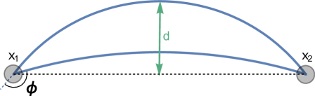
Figure 6: The 2-cusp correlator. For regularisation we cut an $\epsilon$-ball around each of the cusps. The configuration is parameterised by the external angle $\phi$. The result does not depend on $d$ (or equivalently $\chi$ in (3.3)) and is only a function of $x_{12}=|x_{1}-x_{2}|,\;\phi,\;\Delta$ and the regulator $\epsilon$.

In order to compute this quantity we need to work out which cut-offs in the parameters $s$ and $t$ appearing in (3.4) correspond to the $\epsilon$-regularisation. By imposing

$$|\zeta_{+}(-\Lambda_{1})-z_{1}|=\epsilon\;\;,\;\;|\zeta_{+}(\Lambda_{3})-z_{2}|=\epsilon\;\;,\;\;|\zeta_{-}(+\Lambda_{2})-z_{1}|=\epsilon\;\;,\;\;|\zeta_{-}(-\Lambda_{4})-z_{2}|=\epsilon$$ (3.22)

we find (asymptotically for small $\epsilon$)

$$\Lambda_{1}=\Lambda_{2}=\Lambda_{3}=\Lambda_{4}=\log\left(\frac{x_{12}}{\epsilon}\right),\;\;\;\;x_{12}=|z_{1}-z_{2}|,$$ (3.23)

which allows us to write, using (3.21)

$$\langle W_{\epsilon,x_{1},x_{2}}\rangle = G(\Lambda,\Lambda,\Lambda,\Lambda)\simeq\frac{2F^{2}_{0}(0)e^{2\sqrt{-E_{0}}\Lambda}}{||F_{0}||^{2}\sqrt{-E_{0}}}=-\frac{2F^{2}_{0}(0)}{||F_{0}||^{2}\Delta_{0}}\left(\frac{\epsilon}{x_{12}}\right)^{2\Delta_{0}}\;$$ (3.24)

where we use that for large $\Lambda$ only the ground state contributes. We use the notation

$$\Delta_{0}\equiv-\sqrt{-E_{0}}\;$$ (3.25)

so that $\Delta_{0}$ is the usual cusp anomalous dimension. We see that the result for the $2$-cusp correlator takes the standard form $\frac{{\cal N}_{\hat{g},\phi}^{2}}{x_{12}^{2\Delta_{0}}}$ with a rather non-trivial normalization coefficient

$${\cal N}_{\hat{g},\phi}=\epsilon^{\Delta_{0}}\frac{F_{0}(0)}{||F_{0}||}\sqrt{\frac{2}{-\Delta_{0}}}\;,$$ (3.26)

which we will use to extract the structure constant from the 3-cusp correlator.

3.3 Relation to Q-functions

Here we describe a direct relation between solutions of the Schrödinger equation and the Q-functions. From the previous section we can identify $\Delta=-\sqrt{-E}$ resulting in

$$F^{\prime\prime}(z)+\frac{2\hat{g}^{2}}{\cosh z+\cos\phi}F(z)=\frac{\Delta^{2}}{4}F(z)\;.$$ (3.27)

In this section we will relate $F(z)$ with $q(u)$. The relation is very similar to that found previously for the $\phi=\pi$ case in Gromov:2016rrp . For $\phi>0$, the map is defined as follows

$$\frac{F(z)}{2\pi}=\,e^{-\Delta z/2}\int_{{\bf|}}\,q(u)\,e^{w_{\phi}(z)\,u}\,\frac{du}{2\pi iu}\ \ ,$$ (3.28)

where

$$e^{iw_{\phi}(z)}=\left(\frac{\cosh{\frac{z-i\phi}{2}}}{\cosh{\frac{z+i\phi}{2}}}\right),$$ (3.29)

and $q(u)\equiv q_{+}(u)$ is one of the solutions of the Baxter equation (2.7), specified by the large $u$ asymptotics $q(u)\simeq u^{\Delta}e^{u\phi}$. We remind that we use the notation $\int_{{\bf|}}$ for the integration along a vertical line shifted to the right from the origin. For negative $\Delta$ the integral in (3.28) converges for any finite $z$, and we can shift the integration contour horizontally, as long as we do not cross the imaginary axis where the poles of $q(u)$ lie. Let us show that if $q$ satisfies the Baxter equation (2.7), then $F(z)$ computed from (3.28) satisfies the Schrödinger equation (3.27). Applying the derivative in $z$ twice to the relation (3.28) we find

$$F^{\prime\prime}(z)-\frac{\Delta^{2}}{4}F(z)$$

$$=\frac{e^{-\Delta z/2}}{2(\cosh(z)+\cos\phi)}\,\int_{{\bf|}}q(u)\,\left((D+D^{-1})+\frac{2\Delta\sin\phi}{u}-2\,\cos\phi\right)[u\,e^{u\,w_{\phi}(z)}]\,du$$ (3.30)

where $D$ represents the shift operator $D[f(u)]=f(u+i)$. Shifting the integration variable and using the Baxter equation (2.7), the rhs of (3.30) simplifies leading to (3.27).

Notice that this relation between the Baxter and Schrödinger equations holds also off-shell, i.e. when $\Delta$ is a generic parameter and the quantization condition (2.9) need not be satisfied. In Appendix B we show that the quantization condition (2.9) is equivalent to the condition that $F(z)$ is a square-integrable function, so that it corresponds to a bound state of the Schrödinger problem.

Reality.

Let us show that the transform (3.28) defines a real function $F(z)$. Here we assume the quantization condition to be satisfied. Taking the complex conjugate of (3.28) we find

$$\frac{F^{*}(z)}{2\pi}=\,e^{-\Delta z/2}\int_{{\bf|}}\,\bar{q}(u)\,e^{w_{\phi}(z)\,u}\,\frac{du}{2\pi iu}.$$ (3.31)

A precise relation between $q(u)$ and $\bar{q}(u)$ is discussed in appendix A. In particular, from (A.36), (A.47) we see that, when the quantization conditions are satisfied,

$$\bar{q}(u)=q(u)+\mathcal{O}(e^{-2\pi u})+\mathcal{O}(e^{-\phi u}),$$ (3.32)

for large $\text{Re}\,u$. Shifting the contour of integration to the right we see that the contribution of the omitted terms in (3.32) is irrelevant, and therefore the integral transforms involving $\bar{q}(u)$ and $q(u)$ are equivalent. This shows that $F^{*}(z)=F(z)$.

Inverse map.

The transform (3.28) can be inverted as follows:

$$\frac{q(u)}{u}=\frac{\sin{\phi}}{2\pi}\,\int_{i\pi-i\phi}^{+\infty}\frac{dz\;e^{\Delta z/2-w_{\phi}(z)u}}{\cosh{z}+\cos\phi}\,\,F(z).$$ (3.33)

The above integral representation converges for $\text{Im}(u)>0$ and $\Delta<0$. Assuming $F(z)$ is a solution to the Schrödinger equation with decaying behaviour $F(z)\sim e^{\Delta z/2}$ at positive infinity $z\rightarrow+\infty$, this map generates the solution to the Baxter equation $q(u)$. When additionally $F(z)$ decays at $z\rightarrow-\infty$, $q(u)$ satisfies the quantization conditions.

Relation to the norm of the wave function.

From the Schrödinger equation (3.27) we can use the standard perturbation theory to immediately write

$$\frac{\partial\Delta}{\partial\hat{g}}=\frac{8\hat{g}}{\Delta}\frac{1}{||F||^{2}}\int\frac{F^{2}(z)}{\cosh z+\cos\phi}dz\ .$$ (3.34)

We will rewrite the numerator in terms of the Q-function. For that we use that $F_{n}(z)$ is either an even or an odd function depending on the level $n$, then we can write $F^{2}(z)=(-1)^{n}F(z)F(-z)$ and then use (3.28). The advantage of writing the product in this way is that the factor $e^{+\Delta z/2}$ in (3.28) cancels giving

$$\frac{1}{4\pi^{2}}\int\frac{F_{n}^{2}(z)}{\cosh z+\cos\phi}=(-1)^{n}\int_{{\bf|}}\frac{du}{2\pi i}\int_{{\bf|}}\frac{dv}{2\pi i}\int_{-\infty}^{\infty}dz\,\frac{q_{n}(u)}{u}\frac{q_{n}(v)}{v}\,\frac{e^{w_{\phi}(-z)\,u}e^{w_{\phi}(+z)\,v}}{{\cosh z+\cos\phi}}\;\;\;\;.$$ (3.35)

Next we notice that the integration in $z$ can be performed explicitly

$$K(u-v)\equiv\int_{-\infty}^{\infty}\frac{e^{w_{\phi}(-z)\,u}e^{w_{\phi}(+z)\,v}}{\cosh z+\cos\phi}dz=\frac{e^{\phi(u-v)}-e^{\phi(v-u)}}{(u-v)\sin\phi}\;.$$ (3.36)

Note that the function $K(u-v)$ is not singular by itself as the pole at $u=v$ cancels. We are going to get rid of the integral in $u$ in (3.35), for that we notice that we can move the contour of integration in $v$ slighly to the right from the integral in $u$, and after that we can split the two terms in $K(u-v)$. The first term $\sim\frac{e^{\phi(u-v)}}{u-v}$ decays for ${\rm Re}\;v\to+\infty$ and we can shift the integration contour in $v$ to infinity, getting zero. Similarly the second term $\sim\frac{e^{\phi(v-u)}}{u-v}$ decays for ${\rm Re}\;u\to+\infty$ and we can move the integration contour in $u$ to infinity, but this time on the way we pick a pole at $u=v$. That is, only this pole contributes to the result giving

$$\frac{1}{4\pi^{2}}\int\frac{F_{n}^{2}(z)}{\cosh z+\cos\phi}=\frac{(-1)^{n}}{\sin\phi}\int_{{\bf|}}\frac{q_{n}^{2}(v)}{v^{2}}\frac{dv}{2\pi i}\;.$$ (3.37)

At the same time, above in (2.17) we have already derived an expression for $\partial\Delta/\partial\hat{g}$ in terms of the Q-function. Comparing it with (3.34) and using (3.37) we conclude that

$$\boxed{\frac{1}{4\pi^{2}}||F_{n}||^{2}=-(-1)^{n}\frac{2}{\Delta_{n}}\int_{{\bf|}}\frac{q_{n}^{2}}{u}\frac{du}{2\pi i}\;.}$$ (3.38)

We will use the relations between $q$ and $F$ to rewrite the 3-cusp correlator in terms of Q-functions in the next section.

4 Three-cusp structure constant

In this section we derive our main result – an expression for the structure constant. First, we compute it for the case when only one of the $3$ couplings is nonzero. We refer to this case as the Heavy-Light-Light (HLL) correlator . Then we generalize the result to two non-zero couplings, this case we call the Heavy-Heavy-Light (HHL) correlator. In both cases we managed to find an enormous simplification when the result is written in terms of the Q-functions. We postpone the Heavy-Heavy-Heavy (HHH) case for future investigation.

4.1 Set-up and parameterization

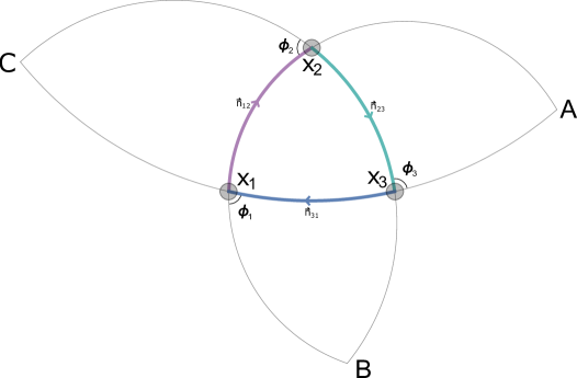
Figure 7: The general configuration of the Wilson loop we consider (the $x_{1}x_{2}x_{3}$ triangle) is built out of $3$ circular arcs belonging to the same plane. The configuration is parameterized by $3$ external angles $\phi_{i}$, coordinates of the vertices $x_{i}$ and $3$ scalar products of the unit vectors attached to the scalars inside the Maldacena-Wilson loop (or equivalently $3$ couplings $\hat{g}_{a}$). Pairs of arcs continued outside the triangle intersect again at $A$, $B$ and $C$. The renormalized 3-cusp correlator has the typical CFT dependence on the positions of the vertices, with a structure constant which depends only on the $3$ angles and $3$ couplings. In this paper we only consider the case with two non-zero couplings.

In this section we describe the $3$-cusp Wilson loop configuration, parameterization and regularisation, which we use in the rest of the paper. The Wilson loop is limited to a 2D plane and consists of $3$ circular arcs coming together at $3$ cusps (see Fig. 7). The $3$ angles $\phi_{i}$, $i=1,2,3$ can be changed independently. The geometry is completely specified by the angles and the positions of the cusps $x_{i}$, $i=1,2,3$.

In the rest of this paper, we consider the following “triangular” inequalities on the angles:

$$\phi_{1}+\phi_{2}>\phi_{3},\,\,\,\phi_{3}+\phi_{2}>\phi_{1},\,\,\,\phi_{3}+\phi_{1}>\phi_{2},\,\,\,0<\phi_{i}<\pi.$$ (4.1)

To understand the geometric meaning of these relations, consider the extension of the arcs forming the Wilson loop past the points $\vec{x}_{i}$: this defines three virtual intersections $A$, $B$, $C$ (see Fig. 7). The inequalities (4.1) mean that $A$, $B$, $C$ are all outside the Wilson loop. Our results will hold in this kinematics regime. In the limit where we approach the boundary of the region (4.1) our result significantly simplifies and will be considered in Sec. 6, in particular we will reproduce the results of Kim:2017sju for the case $\phi_{1}=\phi_{2}=\phi_{3}=0$.

Now we describe a nice way to parametrize the Wilson lines. Consider the two arcs departing from $\vec{x}_{1}$. Extending these arcs past the points $\vec{x}_{2}$, $\vec{x}_{3}$, they define a second intersection point $A$. By making a special conformal transformation, we map $A$ to infinity and both arcs connecting $x_{1}$ with $A$ to straight lines, which we can then map on a cylinder like in (3.3). The most convenient parametrization corresponds to the coordinate along the cylinder. By mapping $A$ back to some finite position we get a rather complicated but explicit parametrization like the one we used in Sec. 3.1.

It is again very convenient to use complex coordinates, similarly to (3.3),

$$\vec{x}=(\text{Re}(z),\text{Im}(z),0,0),$$ (4.2)

so that the cusp points are $\vec{x}_{i}=(\text{Re}(z_{i}),\text{Im}(z_{i}),0,0)$, $i=1,2,3$. For the arcs departing from $z_{1}$ we obtain, as described above, the following representation

$$\zeta_{12}(s) = z_{1}-\frac{z_{12}\,z_{13}\,e^{s}}{e^{s}\,z_{13}+\frac{i}{2\sin\phi_{1}}\,z_{23}\,(1-e^{s})\,(-e^{i\phi_{1}}+e^{-i(\phi_{3}-\phi_{2})})},$$ (4.3)

$$\zeta_{13}(t) = z_{1}-\frac{z_{12}\,z_{13}\,e^{t}}{e^{t}\,z_{12}+\frac{i}{2\sin\phi_{1}}\,z_{23}\,(1-e^{t})\,(-e^{-i\phi_{1}}+e^{-i(\phi_{3}-\phi_{2})})},$$

where $z_{ab}=z_{a}-z_{b}$. Notice that we have slightly redefined the parameters such that $s=0$ and $t=0$ correspond to the other two cusp points: $\zeta_{12}(0)=z_{2}$, $\zeta_{13}(0)=z_{3}$, while $\zeta_{12}(-\infty)=\zeta_{13}(-\infty)=z_{1}$, and $\zeta_{12}(\infty)=\zeta_{13}(\infty)=A$. By a cyclic permutation of all indices, we define similar parametrizations for the other arcs. Notice that, in this way, all arcs are parametrized in two distinct ways, e.g. the same arc connecting $\vec{x}_{1}$ and $\vec{x}_{2}$ is described by the functions $\zeta_{12}(s)$ and $\zeta_{21}(t)$, which are different.

The main advantage of the parametrization (4.3) is that the propagator between the two arcs is very simple:

$$\frac{|\dot{\vec{x}}_{12}(s_{1})||\dot{\vec{x}}_{13}(t_{1})|}{|\vec{x}_{12}(s_{1})-\vec{x}_{13}(t_{1})|^{2}}=\frac{1/2}{\cosh\left(s_{1}-t_{1}-\delta x_{1}\right)+\cos\phi_{1}}\ .$$ (4.4)

However, since we decided to shift the parameters so that $s=0$ gives $\vec{x}_{2}$ and $t=0$ gives $\vec{x}_{3}$, the propagator appears to be shifted compared to (3.8) by the quantity

$$\delta x_{1}=\log\frac{\sin\frac{1}{2}({\phi_{1}}-{\phi_{2}}+{\phi_{3}})}{\sin\frac{1}{2}({\phi_{1}}+{\phi_{2}}-{\phi_{3}})}\;,$$ (4.5)

with $\delta x_{2}$ and $\delta x_{3}$ defined similarly by cyclic permutations of the indices $1,2,3$. We see now the importance of the inequalities (4.1) as they ensure $\delta x_{i}$ are real.

Notation.

Below we consider correlators where the ladder limit is taken independently for the three cusps. Namely, by choosing appropriately polarization vectors $\vec{n}_{i}$ on the three lines, we define effective couplings

$$\hat{g}_{i}^{2}=g^{2}\;\frac{(\vec{n}_{i-1,i}\cdot\vec{n}_{i,i+1})}{2},\;\;\;\;\;\;g\to 0,$$ (4.6)

for the three cusps $i=1,2,3$.

Correspondingly, in this section we use the notation $\Delta_{i,0}$, $i=1,2,3$, to denote the scaling dimensions corresponding to the ground state for the three cusps (in the setup we consider we always have $\hat{g}_{3}=0$, $\Delta_{3,0}=0$). The extension to excited states will be discussed in section 5.

The Q-functions describing the ground state for the first and second cusps will be denoted as $q_{i}(u)$, $i=1,2$, respectively. Explicitly, $q_{i}(u)$ is the solution of the Baxter equation $q_{+}(u)$, evaluated at parameters $\hat{g}=\hat{g}_{i}$, $\Delta=\Delta_{i,0}$ and $\phi=\phi_{i}$.

4.2 Regularization

The $3$ cusp correlator is UV divergent. To regularize the divergence we are going to cut $\epsilon$-circles around each of the cusps – the same way as we regularized the 2-cusp correlator in the previous section. This will set a range for the parameters $s_{i}$ and $t_{i}$ entering the parametrizations $\zeta_{ij}(s_{i})$, $\zeta_{ij}(t_{i})$ defined above. Namely from (4.3) it is easy to find that instead of running from $-\infty$ they now start from a cutoff:

$$s_{i}\in[-\Lambda_{s_{i}},0]\;\;,\;\;t_{i}\in[-\Lambda_{t_{i}},0]$$ (4.7)

where

$$\Lambda_{s_{1}}=\log\left(\frac{x_{12}x_{13}\sin\phi_{1}}{x_{23}\epsilon\sin\left(\frac{1}{2}\left(\phi_{1}-\phi_{2}+\phi_{3}\right)\right)}\right)\;\;,\;\;\Lambda_{t_{1}}=\log\left(\frac{x_{12}x_{13}\sin\phi_{1}}{x_{23}\epsilon\sin\left(\frac{1}{2}\left(\phi_{1}+\phi_{2}-\phi_{3}\right)\right)}\right)\;\;.$$ (4.8)

All other $\Lambda_{s_{i}}$ and $\Lambda_{t_{i}}$ for $i=2,3$, can be obtained by cyclic permutation of the indices $1,2,3$. We note that

$$\Lambda_{s_{i}}+\delta x_{i}=\Lambda_{t_{i}}\;.$$ (4.9)

4.3 Heavy-Light-Light correlator

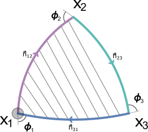
Figure 8: The HLL correlator corresponds to the situation when the couplings $\hat{g}_{2}$ and $\hat{g}_{3}$ are zero. In this case there is only one type of propagators to re-sum.

Now we consider the simplest example of three point function in the ladder limit, where we have only one non-vanishing effective coupling, $\hat{g}_{1}$ for the cusp at $\vec{x}_{1}$, with $\hat{g}_{2}=\hat{g}_{3}=0$. Correspondingly, we will have $\Delta_{2,0}=\Delta_{3,0}=0$, so that this can be considered as a correlator between one nontrivial operator and two protected operators (see Fig. 8). For simplicity we will denote $\Delta_{1,0}$ as just $\Delta_{0}$ in this section.

We start by defining a regularized correlator, which we denote as $Y_{\vec{x}_{1},\epsilon}(\vec{x}_{2},\vec{x}_{3})$, which is obtained by cutting the integration along the Wilson lines at a distance $\epsilon$ from $\vec{x}_{1}$. To compute this observable we consider the sum of all ladder diagrams built around the first cusp and covering the Wilson lines $(12)$, $(13)$ up to the points $\vec{x}_{2}$, $\vec{x}_{3}$, respectively, see Fig. 8. As discussed in section 3, this is described by the Bethe-Salpeter equation, which takes a very convenient form using the parameterization introduced in the previous section for the Wilson lines departing from $\vec{x}_{1}$: $\vec{\gamma}_{12}(s)=(\text{Re}(\zeta_{12}(s)),\text{Im}(\zeta_{12}(s)),0,0)$, and $\vec{\gamma}_{13}(t)=(\text{Re}(\zeta_{13}(t)),\text{Im}(\zeta_{13}(t)),0,0)$. The appropriate integration range for cutting an $\epsilon$-circle around $\vec{x}_{1}$ is $s\in[-\Lambda_{s_{1}},0]$, $t\in[-\Lambda_{t_{1}},0]$, with cutoffs defined in (4.8). However, in order to make a connection with $G(\Lambda_{1},\Lambda_{2},\Lambda_{3},\Lambda_{4})$ defined in section 3, we have to take into account the fact that the propagator in (4.4) is shifted by $\delta x_{1}$. This means that we have to redefine $s\to s+\delta x_{1}$, which will shift the range to $s\in[-\Lambda_{s_{1}}-\delta x_{1},-\delta x_{1}]$, furthermore due to (4.9) the range becomes $s\in[-\Lambda_{t_{1}},-\delta x_{1}]$ . From that we read off the values of $\Lambda_{k}$ and find

$$Y_{\vec{x}_{1},\epsilon}(\vec{x}_{2},\vec{x}_{3})=G(\Lambda_{t_{1}},\Lambda_{t_{1}},-\delta x_{1},0).$$ (4.10)

Again, at large $\Lambda^{\prime}s$ only the ground state survives and we get

$$Y_{\vec{x}_{1},\epsilon}(\vec{x}_{2},\vec{x}_{3})\simeq\frac{2F_{0}(0)F_{0}(\delta x_{1})}{-||F_{0}||^{2}\Delta_{0}}\exp\left(-\Delta_{0}\frac{\Lambda_{t_{1}}+\Lambda_{s_{1}}}{2}\right).$$ (4.11)

Substituting the values for $\Lambda_{t_{1}}$ from (4.8) leads to

$$Y_{\vec{x}_{1},\epsilon}(\vec{x}_{2},\vec{x}_{3})=\frac{2F_{0}(0)F_{0}(\delta x_{1})}{-||F_{0}||^{2}\Delta_{0}}\,\epsilon^{\Delta_{0}}\,\frac{(L_{123})^{{\Delta_{0}}}}{x_{12}^{\Delta_{0}}x_{13}^{\Delta_{0}}x_{23}^{-\Delta_{0}}},$$ (4.12)

which naturally has the structure of the $3$-point correlator in a CFT, where we have defined

$$L_{123}=\frac{\sqrt{\sin\frac{1}{2}(\phi_{1}+\phi_{2}-\phi_{3})\,\sin\frac{1}{2}(\phi_{1}-\phi_{2}+\phi_{3})}}{\sin\phi_{1}}.$$ (4.13)

Finally, to extract the structure constant we have to divide (4.12) by the two point functions normalization (3.26), $\mathcal{N}_{1}=\epsilon^{\Delta_{0}}\frac{F_{0}(0)}{||F_{0}||}\sqrt{\frac{2}{-\Delta_{0}}}$ , so we get:

$$C_{123}^{\bullet\circ\circ}=\left(\frac{-2}{\Delta_{0}\,||F_{0}||^{2}}\right)^{\frac{1}{2}}\,(L_{123})^{{\Delta_{0}}}\;F_{0}(\delta x_{1}).$$ (4.14)

Let us now write the result in terms of the Q-functions. Using (3.28) to evaluate the shifted wave function in (4.14), we already notice a nice simplification:

$$w_{\phi_{1}}(\pm\delta x_{1})=\pm(\phi_{2}-\phi_{3}),$$ (4.15)

therefore (using also parity of the ground-state wave function)

$$F_{0}(-\delta x_{1})=F_{0}(+\delta x_{1})=-i\,e^{-\frac{\delta x_{1}}{2}\,\Delta_{0}}\,\int_{{\bf|}}\frac{q_{1}(u)}{u}\,e^{(\phi_{2}-\phi_{3})u}\,du$$ (4.16)

and taking into account also the norm formula (3.38), we find

$$C^{\bullet\circ\circ}_{123}=\,(K_{123})^{\Delta_{0}}\,\frac{-i\,\int_{{\bf|}}\frac{q_{1}(u)}{u}\,e^{(\phi_{2}-\phi_{3})u}\,du}{\left(-2\pi i\,\int_{{\bf|}}\frac{q_{1}^{2}(u)\,}{u}\,du\right)^{\frac{1}{2}}},$$ (4.17)

where the constant $K_{123}$ is defined as

$$K_{123}=L_{123}\,e^{\frac{\delta x_{1}}{2}}=\frac{\sin\frac{1}{2}(\phi_{1}+\phi_{2}-\phi_{3})}{\sin\phi_{1}}.$$ (4.18)

Using the parity of the ground state wave function $F_{0}$, it can be verified that the result is symmetric in the two angles $\phi_{2}\leftrightarrow\phi_{3}$.

We see that the result takes a much simpler form in terms of the Q-functions. The structure becomes even more clear when written in terms of the bracket ${\langle\!\!\langle}\cdot{\rangle\!\!\rangle}$ defined in (1.4):

$$\boxed{C^{\bullet\circ\circ}_{123}=\frac{{\langle\!\!\langle}q_{1}e^{u(\phi_{2}-\phi_{3})}{\rangle\!\!\rangle}}{\sqrt{{\langle\!\!\langle}q_{1}^{2}{\rangle\!\!\rangle}}}}\;,$$ (4.19)

which is amazingly simple!

4.4 Heavy-Heavy-Light correlator

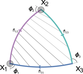
Figure 9: The HHL correlator. In this case there are two types of propagators since two couplings are non-zero.

Now, we switch on the effective couplings $\hat{g}_{i}$, $i=1,2$ for both the first and the second cusp. This means that this observable is defined perturbatively by Feynman diagrams with two kinds of ladders built around the cusps $\vec{x}_{1}$ and $\vec{x}_{2}$, see Fig. 9.

As in the previous section let us denote by $Y_{\vec{x}_{1},\epsilon}(\vec{x}_{2},\vec{x}_{3})$ the sum of all ladders built around the cusp point $\vec{x}_{1}$, with a cutoff at distance $\epsilon$ from the cusp. We introduce a similar notation for the ladders built around the second cusp.

The sum of all diagrams contributing to the $\epsilon$-regularized Heavy-Heavy-Light correlator can be organized as follows:

$$\begin{array}[]{rccccc}W^{{\bullet\bullet\circ},\,\epsilon}_{123}&=&\underbrace{\sum\limits_{\text{propagators only around $2$}}}_{Y_{\vec{x}_{2},\epsilon}(\vec{x}_{3},\vec{x}_{1})}&+&\underbrace{\sum\limits_{\text{diagrams with at least one propagator around $1$}}}_{\left(W^{{\bullet\bullet\circ},\epsilon}_{123}\right)_{1}}\end{array}$$ (4.20)

where the part $\left(W^{{\bullet\bullet\circ},\epsilon}_{123}\right)_{1}$ represents the sum of all diagrams with at least one propagator around the cusp $x_{1}$. As we are about to show, the leading UV divergence comes only from the connected part, which behaves as $\sim\epsilon^{\Delta_{1,0}+\Delta_{2,0}}$. Since the disconnected contributions in (4.21) have a milder divergence $\sim\epsilon^{\Delta_{i,0}}$ $(i=1,2)$, we can drop them since they are irrelevant to the definition of the renormalized structure constant.

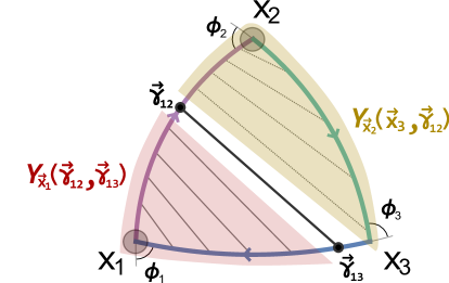
Figure 10: We split the propagators into two groups by explicitly writing the last propagator between $\vec{\gamma}_{12}$ and $\vec{\gamma}_{13}$. Then we re-sum the propagators surrounding cusp $x_{2}$ into $Y_{\vec{x}_{2}}(\vec{x}_{3},\vec{\gamma}_{12})$ and those around $x_{1}$ into $Y_{\vec{x}_{1}}(\vec{\gamma}_{12},\vec{\gamma}_{13})$.

As illustrated in Fig. 10, the main contribution can be computed as follows:

$$\left(W^{{\bullet\bullet\circ},\epsilon}_{123}\right)_{1}=\int_{\vec{x}_{1}+O(\epsilon)}^{\vec{x}_{2}+O(\epsilon)}d|\vec{\gamma}_{12}|\int_{\vec{x}_{1}+O(\epsilon)}^{\vec{x}_{3}}d|\vec{\gamma}_{13}|\;Y_{\vec{x}_{1},\epsilon}(\vec{\gamma}_{12},\vec{\gamma}_{13})\,\frac{1}{|\vec{\gamma}_{12}-\vec{\gamma}_{13}|^{2}}\,Y_{\vec{x}_{2},\epsilon}(\vec{x}_{3},\vec{\gamma}_{12}),$$

(4.21)

where we are denoting with $Y_{\vec{x}_{1},\epsilon}(\vec{\gamma}_{12},\vec{\gamma}_{13})$ the sum of all ladder diagrams up to the points $\vec{\gamma}_{12}$, $\vec{\gamma}_{13}$ on the arcs $(12)$, $(13)$, respectively (and similarly for $Y_{\vec{x}_{2},\epsilon}(\vec{x}_{3},\vec{\gamma}_{12})$).

To compute the connected integral explicitly we choose the following parametrization for the arcs $(12)$, $(13)$:

$$\vec{\gamma}_{12}(s) = \left(\text{Re}(\zeta_{12}(s)),\text{Im}(\zeta_{12}(s)),0,0\right),$$ (4.22)

$$\vec{\gamma}_{13}(t) = \left(\text{Re}(\zeta_{13}(t)),\text{Im}(\zeta_{13}(t)),0,0\right),$$ (4.23)

where the functions $\zeta_{ij}$ are again the ones we defined above in section  4.1. The function $Y_{\vec{x}_{1},\epsilon}(\vec{\gamma}_{12}(s);\vec{\gamma}_{13}(t))$ is given by the solution to the Bethe-Salpeter equation with shifted propagator (4.4), where the integration range is $s_{1}\in[-\Lambda_{s_{1}},s]$, $t_{1}\in[-\Lambda_{t_{1}},t]$. Exactly as described in section 4.3, redefining the parameters we find, in terms of the amputated four point function $G(\Lambda_{1},\dots,\Lambda_{4})$:

$$Y_{\vec{x}_{1},\epsilon}(\vec{\gamma}_{12}(s);\vec{\gamma}_{13}(t))=G_{1}(\Lambda_{t_{1}},\Lambda_{t_{1}},s-\delta x_{1},0),$$ (4.24)

where $\delta x_{1}$ is defined in (4.5), and for $\epsilon\rightarrow 0$ we have

$$Y_{\vec{x}_{1},\epsilon}(\vec{\gamma}_{12}(s);\vec{\gamma}_{13}(t))\sim\left(\frac{2F_{1,0}(0)}{-||F_{1,0}||^{2}\Delta_{1,0}}\right)\,\left(\frac{\epsilon\,L_{123}\;x_{23}}{x_{12}\,x_{13}}\right)^{\Delta_{1,0}}\,e^{-\frac{s+t}{2}\,\Delta_{1,0}}\,F_{1,0}(-\delta x_{1}+s-t),$$ (4.25)

where $L_{123}$ is defined in (4.5).

The other ingredient appearing in (4.21) is $Y_{\vec{x}_{2},\epsilon}(\vec{x}_{3},\vec{\gamma_{12}}(s))$. Computing this quantity is slightly more complicated, since the ladders built around the second cusp point $\vec{x}_{2}$ are described most naturally in terms of a different parametrization, which uses the functions $\zeta_{21}(t_{2})$, $\zeta_{23}(s_{2})$ to parametrize the arcs $(12)$, $(23)$. In fact, it is only in the variables $s_{2}$ and $t_{2}$ that the propagator takes the simple form (4.4), with $\delta x_{1}\rightarrow\delta x_{2}$. Therefore we need to relate the two alternative parametrizations, $\zeta_{21}(t_{2})$ vs $\zeta_{12}(s_{1})$, for the line $(12)$. To this end we introduce the transition map $T_{12}(s)$:

$$\zeta_{12}(s)=\zeta_{21}(T_{12}(s)),$$ (4.26)

which is given explicitly by

$$e^{T_{12}(s)}=\frac{(1-e^{s})}{1-e^{s}\frac{\cos\phi_{3}-\cos(\phi_{1}+\phi_{2})}{\cos\phi_{3}-\cos(\phi_{1}-\phi_{2})}\,}.$$ (4.27)

Using this map, we find that $Y_{\vec{x}_{2},\epsilon}(\vec{x}_{3},{\vec{\gamma}_{12}}(s))$ is defined by the Bethe-Salpeter equation with propagator shifted by $\delta x_{2}$ and integration ranges $s_{2}\in[-\Lambda_{s_{2}},0]$, $t_{2}\in[-\Lambda_{t_{2}},T_{12}(s)]$. Taking into account the shift in the propagator, we have

$$Y_{\vec{x}_{2},\epsilon}(\vec{x}_{3},{\vec{\gamma}_{12}}(s))=G_{2}(\Lambda_{t_{2}},\Lambda_{t_{2}},-\delta x_{2},T_{12}(s)),$$ (4.28)

which for small $\epsilon$ yields

$$Y_{\vec{x}_{2},\epsilon}(\vec{x}_{3},\vec{\gamma_{12}}(s))\sim\left(\frac{2F_{2,0}(0)}{-||F_{2,0}||^{2}\Delta_{2,0}}\right)\,\left(\frac{\epsilon\;L_{231}\;x_{13}}{x_{23}\,x_{12}}\right)^{\Delta_{2,0}}\,e^{-\frac{T_{12}(s)}{2}\,\Delta_{2,0}}\,F_{2,0}(-\delta x_{2}-T_{12}(s)),$$ (4.29)

where $L_{231}$ is defined applying a cyclic permutation to (4.18). Combining (4.25), (4.29) in (4.21), we find, for the leading divergent part:

$$W^{\bullet\bullet\circ,\,\epsilon}_{123}=\frac{\epsilon^{\Delta_{1,0}+\Delta_{2,0}}(L_{123})^{\Delta_{1,0}}\,(L_{231})^{\Delta_{2,0}}}{x_{12}^{\Delta_{1,0}+\Delta_{2,0}}\,x_{13}^{\Delta_{1,0}-\Delta_{2,0}}\,x_{23}^{\Delta_{2,0}-\Delta_{1,0}}}\,\left(\frac{4\,F_{2,0}(0)F_{1,0}(0)}{||F_{1,0}||^{2}\,||F_{2,0}||^{2}\,\Delta_{1,0}\,\Delta_{2,0}}\right)\,\;\mathcal{N}^{\bullet\bullet\circ}_{123},$$ (4.30)

where $\mathcal{N}_{123}^{\bullet\bullet\circ}$ is a finite constant which can be written explicitly as

$$\mathcal{N}_{123}^{\bullet\bullet\circ} = 2\hat{g}_{1}^{2}\,\int_{-\infty}^{0}ds\,\int_{-\infty}^{0}dt\,\frac{F_{1,0}(-\delta x_{1}+s-t)\,F_{2,0}(-\delta x_{2}-T_{12}(s))\,e^{-\frac{s+t}{2}\,\Delta_{1,0}-\frac{T_{12}(s)}{2}\,\Delta_{2,0}}}{\cosh(s-t-\delta x_{1})+\cos\phi_{1}}.$$

Again, we see that (4.30) has the correct space-time dependence for a CFT 3-point correlator. Normalizing by the 2-pt functions factors $\mathcal{N}_{\Delta_{i},\phi_{i}}$ defined in (3.26) for the two cusps, we get a finite expression for the structure constant:

$$C^{\bullet\bullet\circ}_{123}=2\,\frac{(L_{123})^{\Delta_{1,0}}\,(L_{231})^{\Delta_{2,0}}}{\sqrt{\Delta_{1,0}\,\Delta_{2,0}}\,||F_{1,0}||\,||F_{2,0}||}\,\mathcal{N}_{123}^{{\bullet\bullet\circ}}.$$ (4.32)

Using the Schrödinger equation for $F_{1,0}$, we can simplify the expression for $\mathcal{N}_{123}^{\bullet\bullet\circ}$ further and remove one of the integrations:

$$\mathcal{N}_{123}^{\bullet\bullet\circ} = \int_{-\infty}^{0}ds\,\int_{-\infty}^{0}dt\,\partial_{s}\partial_{t}\,\left(F_{1,0}(-\delta x_{1}+s-t)\,e^{-\frac{s+t}{2}\,\Delta_{1,0}}\right)\,F_{2,0}(-\delta x_{2}-T_{12}(s))\,e^{-\frac{T_{12}(s)}{2}\,\Delta_{2,0}}$$ (4.33)

$$= \int_{-\infty}^{0}ds\,\partial_{s}\left(F_{1,0}(-\delta x_{1}+s)\,e^{-\frac{s}{2}\,\Delta_{1,0}}\right)\,F_{2,0}(\,-\delta x_{2}-T_{12}(s)\,)\,e^{-\frac{T_{12}(s)}{2}\,\Delta_{2,0}}.$$

While (4.33) provides an explicit result, it still appears rather intricate, especially since it contains the complicated transition function $T_{12}(s)$. We will now show that it can be reduced to an amazingly simple form in terms of the Q-functions.

First, applying the transform (3.28), and using parity of the ground state wave function, $F_{1,0}(z)=F_{1,0}(-z)$, we can write

$$F_{1,0}(s-\delta x_{1})\,e^{-\frac{s-\delta x_{1}}{2}\Delta_{1,0}} = -i\int_{{\bf|}}\frac{du}{u}\,q_{1}(u)\times\text{exp}\left(u\,w_{\phi_{1}}(\delta x_{1}-s)\right),$$ (4.34)

$$F_{2,0}(-\delta x_{2}-T_{12}(s))\,e^{-\frac{T_{12}(s)+\delta x_{2}}{2}\Delta_{2,0}} = -i\int_{{\bf|}}\frac{du}{u}\,q_{2}(u)\times\text{exp}\left(u\,w_{\phi_{2}}(-T_{12}(s)-\delta x_{2})\right).$$

We then plug these relations into (4.33). We noticed a magic relation between the integrands of (4.34) and (LABEL:eq:inteF2),

$$w_{\phi_{1}}(s-\delta x_{1})=w_{\phi_{2}}(-\delta x_{2}-T_{12}(s))-\phi_{3}\ \ ,$$ (4.36)

which suggests that we switch to a new integration variable $\xi=w_{\phi_{1}}(s-\delta x_{1})-\phi_{3}/2$. Notice that the integration measure is invariant, $ds\,\partial_{s}=d\xi\,\partial_{\xi}$. Taking into account (4.36) we get:

$$\mathcal{N}_{123}^{\bullet\bullet\circ} = -e^{\frac{\delta_{12}}{2}}\,\int_{{\bf|}}\frac{du}{u}\int_{{\bf|}}\frac{dv}{v}\,q_{1}(u)\,q_{2}(v)\,\left[\int^{-\phi_{2}+\phi_{3}/2}_{\phi_{1}-\phi_{3}/2}d\xi\,\partial_{\xi}\left(e^{-u\xi-u\phi_{3}/2}\right)\,e^{v\xi-v\,\phi_{3}/2}\right],$$

$$\delta_{12} = -{\delta x_{1}}{}\,\Delta_{1,0}+{\delta x_{2}}{}\,\Delta_{2,0}\ \ ,$$ (4.37)

and remarkably we can do the integral explicitly and find

$$\mathcal{N}_{123}^{\bullet\bullet\circ}=e^{\frac{\delta_{12}}{2}}\,\int_{{\bf|}}du\,\int_{{\bf|}}\frac{dv}{v}\,q_{1}(u)\,q_{2}(v)\,\left(\frac{e^{(\phi_{2}-\phi_{3})u-\phi_{2}v}-e^{-\phi_{1}\,u+(\phi_{1}-\phi_{3})v}}{u-v}\right).$$ (4.38)

We can simplify this expression further. In fact, notice that the integrand has no poles for $\text{Re}(u)>0$, $\text{Re}(v)>0$, in particular there is no pole at $u\sim v$. Therefore we can shift the two integration contours independently. Similarly to the trick used in section 3.3, we shift the $v$ integration contour to the right so that $\text{Re}(v)>\text{Re}(u)$, and split the integral into two contributions. One of them vanishes since the $v$-integrand is suppressed and the integration contour can be closed at $\text{Re}(v)=\infty$:

$$\int_{{\bf|}}du\,q_{1}(u)\,e^{(\phi_{2}-\phi_{3})u}\,\left(\int_{{{\bf|}}\,+0^{+}}\frac{dv}{v}\,q_{2}(v)\,\frac{e^{-\phi_{2}v}}{u-v}\right)=0,$$ (4.39)

while for the second integral it is the $u$-integrand that is suppressed. Closing the contour we now pick a residue at $u\sim v$:

$$\mathcal{N}^{\bullet\bullet\circ}_{123} = -e^{\frac{\delta_{12}}{2}}\,\int_{{{\bf|}}\,\,+\,0^{+}}\frac{dv}{v}\,q_{2}(v)\,e^{(\phi_{1}-\phi_{3})v}\,\left(\int_{{\bf|}}du\,\frac{q_{1}(u)\,e^{-\phi_{1}u}}{u-v}\right)$$ (4.40)

$$= +e^{\frac{\delta_{12}}{2}}\,(2\pi i)\int_{{\bf|}}\frac{dv}{v}\,q_{1}(v)\,q_{2}(v)\,e^{-\phi_{3}v}.$$ (4.41)

Combining all ingredients, we get the final expression for the structure constant in terms of the Q functions:

$$C^{\bullet\bullet\circ}_{123}=(K_{123})^{\Delta_{1,0}}\,(K_{213})^{\Delta_{2,0}}\,\frac{\,\int_{{\bf|}}\,q_{1}\,q_{2}\,e^{-\phi_{3}u}\frac{du}{2\pi iu}}{\sqrt{\int_{{\bf|}}q_{1}\,{q}_{1}\,\frac{du}{2\pi iu}}\ \,\sqrt{\int_{{\bf|}}q_{2}\,{q}_{2}\,\frac{du}{2\pi iu}}},$$ (4.42)

where the constants $K_{123}$, $K_{213}$ are defined as in (4.18) by permutation of the indices. Again, it simplifies further in terms of the bracket ${\langle\!\!\langle}\cdot{\rangle\!\!\rangle}$ defined in (1.4)

$$\boxed{C^{\bullet\bullet\circ}_{123}=\,\frac{\,{\langle\!\!\langle}q_{1}\,q_{2}\,e^{-\phi_{3}u}{\rangle\!\!\rangle}}{\sqrt{{\langle\!\!\langle}q_{1}^{2}{\rangle\!\!\rangle}{\langle\!\!\langle}q_{2}^{2}{\rangle\!\!\rangle}}}}\ \ .$$ (4.43)

In this form it is clear that the final expression is explicitly symmetric for $1\leftrightarrow 2$, even though for the derivation we treated cusp $x_{1}$ differently from $x_{2}$.

This strikingly compact expression is one of our main results. Notice that it also covers the HLL case, namely if we send one of the effective couplings $\hat{g}_{1},\hat{g}_{2}$ to zero we recover (4.19) as for zero coupling ${\langle\!\!\langle}q^{2}{\rangle\!\!\rangle}=1$.

5 Excited states

In this section we explore the meaning of the excited states and give them a QFT interpretation as insertions at the cusps. We will also extend our result for the structure constant to the excited states.

Figure 11: Structure of the spectrum of the Schrodinger operator. For finite coupling there are finitely many bound states. When the coupling is decreased, eventually the top bound state touches the continuum and goes to another sheet, becoming a resonance. There are infinitely many resonances for any value of the coupling. The spectrum of dimensions is related to the energy of the Schrodinger equation by $\Delta=-\sqrt{-E}$. This map resolves the branch cut of the continuum spectrum making the bound states and the resonances indistinguishable and equally important.

5.1 Excited states and insertions

First, let us discuss the structure of the spectrum of the Schrödinger equation. When we increase the coupling we find more and more bound states in the spectrum at $E<0$. If we analytically continue the bound state energy by slowly decreasing the coupling we will find that the level approaches the continuum at $E=0$ and then reflects back. After that point the state will strictly speaking disappear from the spectrum of the bound states as the wave function will no longer be normalizable. However, if we define the bound state as a pole of the resolvent, it will continue to be a pole, just not on the physical sheet, but under the cut of the continuum part of the spectrum.

At the same time, from the expression for $G(\Lambda_{1},\Lambda_{2},\Lambda_{3},\Lambda_{4})$ in (3.21) we see that the natural variable is not $E$ but rather $\Delta=-\sqrt{-E}$. In the $\Delta$-plane the branch cut of the continuum spectrum will open revealing all the infinite number of the resonances bringing them back into the physical spectrum (see Fig. 12).

Figure 12: Structure of the spectrum of the QSC. The map $\Delta=-\sqrt{-E}$, which relates the spectrum obtained from QSC to the Schrodinger equation, resolves the cut of the continuum spectrum, revealing an infinite set of states.

In order to give the field theory interpretation of those bound states we build projectors, which acting on our main object $G(\Lambda_{1},\Lambda_{2},\Lambda_{3},\Lambda_{4})$ will project on the excited states $\Delta_{n}$ in the large $\Lambda_{i}$ limit. First let us rewrite (3.21) in terms of $\Delta_{n}$’s

$$G(\Lambda_{1},\Lambda_{2},\Lambda_{3},\Lambda_{4})\simeq\sum_{n}\frac{2F_{n}(\Lambda_{1}-\Lambda_{2})F_{n}(\Lambda_{4}-\Lambda_{3})}{||F_{n}||^{2}(-\Delta_{n})}\exp\left(-\Delta_{n}\frac{\Lambda_{1}+\Lambda_{2}+\Lambda_{3}+\Lambda_{4}}{2}\right)\;.$$ (5.1)

Since $G$ has an interpretation as a $4$-BPS correlator, one can think about (5.1) as an OPE expansion in the $t$-channel. We will also see soon that the coefficients appearing there are the HLL structure constants with excited states. We will come back to this point in section 9.

When $\Lambda$’s tend to infinity the sum is saturated by the smallest $\Delta_{n}$. To suppress the lowest states we define the following differential operators:

$${\cal O}_{2m}=\prod_{i=0}^{m-1}\frac{\partial_{+}+\Delta_{2i}}{-\Delta_{2m}+\Delta_{2i}}\;\;,\;\;{\cal O}_{2m+1}=\prod_{i=0}^{m-1}\frac{\partial_{+}+\Delta_{2i+1}}{-\Delta_{2m+1}+\Delta_{2i+1}}\times\frac{1}{2}\partial_{-}$$ (5.2)

where $\partial_{\pm}\equiv\partial_{\Lambda_{1}}\pm\partial_{\Lambda_{2}}\;\;,\;\;\bar{\partial}_{\pm}\equiv\partial_{\Lambda_{4}}\pm\partial_{\Lambda_{3}}$. With the help of these operators we define

$$W_{n} \equiv \left.{\cal O}_{n}\bar{\cal O}_{n}\,G(\Lambda_{1},\Lambda_{2},\Lambda_{3},\Lambda_{4})\right|_{\Lambda_{1}=\Lambda,\;\Lambda_{2}=\Lambda,\;\Lambda_{3}=\Lambda,\;\Lambda_{4}=\Lambda}\;,$$ (5.3)

which at large $\Lambda$ scales as $e^{-2\Delta_{n}\Lambda}$ since all terms with $k<n$ are projected out! Notice that, as discussed in Sec. 3.2, $G(\Lambda,\Lambda,\Lambda,\Lambda)$ can be used to describe a regularized two-point function, where the cutoff is identified with $x_{12}e^{-\Lambda}=\epsilon$, similarly we get

$$W_{2m}\simeq\left(\frac{\epsilon}{x_{12}}\right)^{2\Delta_{2m}}\frac{-2[F_{2m}(0)]^{2}}{||F_{2m}||^{2}\,\Delta_{2m}}\;\;,\;\;W_{2m+1}\simeq\left(\frac{\epsilon}{x_{12}}\right)^{2\Delta_{2m+1}}\frac{-2[F^{\prime}_{2m+1}(0)]^{2}}{||F_{2m+1}||^{2}\,\Delta_{2m+1}},$$ (5.4)

which indeed has the structure of the two point function of operators with dimension $\Delta_{n}$! These are the two point functions of the cusps with extra insertions due to the action of ${\cal O}_{n}$. The specific form of the operator insertion in general depends on the regularization scheme. The operators ${\cal O}_{n}$ give an explicit form of these insertions for the point-splitting regularization. For instance, the first two operators ${\cal O}_{1}=\frac{1}{2}\partial_{-}$ and ${\cal O}_{2}=\frac{\partial_{+}+\Delta_{0}}{\Delta_{0}-\Delta_{2}}$ will produce the following insertions

$${\cal O}_{1}\;\; \leftrightarrow \;\;\frac{1}{2}\left(-\Phi^{a}n_{2}^{a}|\dot{x}(\Lambda_{2})|+\Phi^{a}n_{1}^{a}|\dot{x}(-\Lambda_{1})|\right)=\left(\Phi^{a}n_{1}^{a}-\Phi^{a}n_{2}^{a}\right)\frac{\epsilon}{2}\;,$$ (5.5)

$${\cal O}_{2}\;\; \leftrightarrow \;\;\frac{(\Phi^{a}n_{2}^{a}+\Phi^{a}n_{1}^{a})\epsilon+\Delta_{0}}{\Delta_{0}-\Delta_{2}}\;.$$ (5.6)

Naively, the interpretation of the operators corresponding to the excited states is only valid for large enough coupling when $\Delta_{n}<0$. In the next section we verify that it remains true at weak coupling at one loop level.

Below, we also extend our result for the 3-cusp correlator to excited states. For this, we will need to know the long-time asymptotics of $\tilde{G}_{\Lambda_{1},\Lambda_{2}}(x,y)$ computed with the new type of boundary conditions described by the action of the projector $\mathcal{O}_{n}$. We have, for $y\rightarrow\infty$,

$$\mathcal{O}_{n}\,\tilde{G}_{\Lambda_{1},\Lambda_{2}}(x,y)\simeq c_{n}F_{n}(x)\;e^{-\Delta_{n}y},$$ (5.7)

where

$$c_{2m}=-\frac{2F_{2m}(0)}{||F_{2m}||^{2}\,\Delta_{2m}}\;\;,\;\;c_{2m+1}=-\frac{2F^{\prime}_{2m+1}(0)}{||F_{2m+1}||^{2}\,\Delta_{2m+1}}\;.$$ (5.8)

Finally, from the $2$-point correlator (5.4) we extract the normalization coefficients

$${\cal N}_{\Delta_{n}}=\epsilon^{\Delta_{n}}\,c_{n}\,\sqrt{\frac{-\Delta_{n}\,||F_{n}||^{2}}{2}},$$ (5.9)

which we will need to normalize the structure constant in the next section.

5.2 Correlator with excited states

We will redo the calculation of the HLL correlator for the case when the heavy state is excited. We mostly notice that all the steps are essentially the same as in the case of the ground state. We begin by applying the projector operator ${\cal O}_{n}$, defined in (5.2) to the cusp at $x_{1}$ and use that in the small $\epsilon$ limit we simply use the leading asymptotics (5.7) to obtain, very similarly to the ground state (4.10)

$${\cal O}_{n}Y_{\vec{x}_{1},\epsilon}(\vec{x}_{2},\vec{x}_{3})=c_{n}\,F_{n}(-\delta x_{1})\,\epsilon^{\Delta_{n}}\,\frac{(L_{123})^{{\Delta_{n}}}}{x_{12}^{\Delta_{n}}x_{13}^{\Delta_{n}}x_{23}^{-\Delta_{n}}},$$ (5.10)

with $c_{n}$ defined in (5.8). Normalizing the result with (5.9) to get a finite result for the structure constant we get

$$C_{123}^{\bullet_{n}\circ\circ}=\sqrt{\frac{2}{-\Delta_{n}||F_{n}||^{2}}}\,{F_{n}(\delta x_{1})}\,(L_{123})^{{\Delta_{n}}}\;.$$ (5.11)

rewriting it in terms of q-functions exactly as for the ground state we obtain

$$\boxed{C^{\bullet_{n}\circ\circ}_{123}=\frac{{\langle\!\!\langle}q_{1,n}e^{\phi_{2}u-\phi_{3}u}{\rangle\!\!\rangle}}{\sqrt{(-1)^{n}{\langle\!\!\langle}q_{1,n}^{2}{\rangle\!\!\rangle}}}}\;,$$ (5.12)

where $q_{1,n}$ denotes the solution of the QSC corresponding to the $n$-th excited state, with parameters $\hat{g}=\hat{g}_{1}$, $\phi=\phi_{1}$. The $(-1)^{n}$ appears from the corresponding factor in the relation for the norm of the wavefunction in (3.38), it is needed to ensure the denominator is real at large couplings.

Similarly for the HHL correlator we simply replace q-functions and the corresponding dimensions, but the expression stays the same!

$$\boxed{C^{\bullet_{n}\bullet_{m}\circ}_{123}=\frac{(-1)^{m}{\langle\!\!\langle}q_{1,n}q_{2,m}e^{-\phi_{3}u}{\rangle\!\!\rangle}}{\sqrt{(-1)^{n+m}{\langle\!\!\langle}q_{1,n}^{2}{\rangle\!\!\rangle}{\langle\!\!\langle}q_{2,m}^{2}{\rangle\!\!\rangle}}}}\;.$$ (5.13)

5.3 Excited states at weak coupling from QSC

As we discussed above (see section 3), for large coupling the Schrödinger equation has several bound states while for small coupling all of them except the ground state disappear. Nevertheless the excited states have remnants at weak coupling which are not immediately apparent in the Schrödinger equation but are directly visible in the QSC. By solving the Baxter equation (2.7) and the gluing condition (2.9) numerically, we can follow any excited state from large to small coupling and we find that $\Delta$ has a perfectly smooth dependence on $\hat{g}$. The first several states are shown on Fig. 13 and Fig. 14 which also demonstrate an intricate pattern of level crossings that we will discuss below. For $\hat{g}\to 0$ we moreover observe that $\Delta$ becomes a positive integer $L$,

$$\Delta=L+\Delta^{(1)}\hat{g}^{2}+\Delta^{(2)}\hat{g}^{4}+\dots,\ \ \ \ L=1,2,\dots\ \ .$$ (5.14)

Remarkably, for each $L>0$ we have two states which become degenerate at zero coupling. In contrast, the ground state (corresponding to $L=0$) does not merge with any other state. This pattern is consistent with our proposal for the insertions (5.2) – the states with $n=2m$ and $n=2m-1$ have the same number of derivatives and thus should have the same bare dimension.

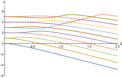
Figure 13: The first few states for $\phi=1.5\,\,$. We show numerical data for $\Delta$ as a function of $\hat{g}$, obtained from the Baxter equation. We see that all the states, except the ground state, are paired together at weak coupling.

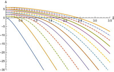
Figure 14: The first few states for $\phi=3.0\,\,$. We plot $\Delta$ as a function of the coupling $\hat{g}$ similarly to Fig. 13.

We can explicitly compute $\Delta$ for these states at weak coupling from the Baxter equation. We solve it perturbatively using the efficient iterative method of Gromov:2015vua and the Mathematica package provided with Gromov:2015dfa . We start from the solution at $\hat{g}=0$ and improve it order by order in $\hat{g}$. At $\hat{g}=0$ the solution for any $L\equiv\left.\Delta\right|_{\hat{g}=0}$ has the form of a polynomial of degree $L$ multiplied by $e^{u\phi}$. At the next order we already encounter nontrivial pole structures. This procedure gives $q$-functions written in terms of generalized $\eta$-functions Marboe:2014gma ; Gromov:2015dfa defined as

$$\eta_{s_{1},\dots,s_{k}}^{z_{1},\dots,z_{k}}(u)\equiv\sum_{n_{1}>n_{2}>\dots>n_{k}\geq 0}\frac{z_{1}^{n_{1}}\dots z_{k}^{n_{k}}}{(u+in_{1})^{s_{1}}\dots(u+in_{k})^{s_{k}}}\ .$$ (5.15)

As an example, for $L=1$ we find

$$q=e^{u\phi}\left[u+\hat{g}^{2}\left(-i\Delta^{(1)}u\;\eta_{1}^{1}-\frac{2}{\sin\phi}+\frac{\Delta^{(1)}}{2}(-2ue^{2i\phi}+\cot\phi+i)\right)\right]+\mathcal{O}(\hat{g}^{4})$$ (5.16)

where $\Delta^{(1)}$ is the 1-loop coefficient in (5.14). The second solution $q_{-}$ is more complicated and already involves twisted $\eta$-functions such as $\eta_{1}^{e^{2i\phi}}$, but fortunately we only need $q_{+}$ to close the equations. The quantization condition (2.9) then gives a quadratic equation on $\Delta^{(1)}$ which fixes

$$\Delta^{(1)}=\pm 4\ \ \ \text{for}\ \ \ L=1\ .$$ (5.17)

Thus as expected from the numerical analytsis we find two separate states, which become degenerate at zero coupling.

For comparison, for the ground state ($L=0$) we have

$$q=e^{u\phi}\,\left[1+\hat{g}^{2}\,\frac{2i}{\sin\phi}\,\left(2\,\phi\,(\eta^{1}_{1}-\eta^{e^{2i\phi}}_{1})-(\eta^{1}_{2}-\eta^{e^{2i\phi}}_{2})\right)\right]+\mathcal{O}(\hat{g}^{4})\ .$$ (5.18)

Repeating this calculation for $L=2,3,4,5$ we were able to guess a simple closed formula for the 1-loop correction,

$$\Delta_{L,\pm}=L\pm\frac{4}{L}\frac{\sin L\phi}{\sin\phi}\hat{g}^{2}+\dots,\ \ \ \ L=1,2,\dots\;.$$ (5.19)

For the ground state ($L\to 0$) this formula also gives the correct result although only the minus sign is admissible.

For the first several states we also computed $\Delta$ to two loops, e.g. for $L=1$

$$\Delta_{1,-} = 1-4\hat{g}^{2}+16\left(\phi\cot\frac{\phi}{2}-1\right)\hat{g}^{4}+\dots$$ (5.20)

$$\Delta_{1,+} = 1+4\hat{g}^{2}-16\left(\phi\tan\frac{\phi}{2}+1\right)\hat{g}^{4}+\dots\;.$$ (5.21)

The two-loop results for $L=2,3$ are given in Appendix C. All these results are also in excellent agreement with QSC numerics. For completeness, the ground state anomalous dimension to two loops is Makeenko:2006ds ; Drukker:2011za

$$\Delta_{0} = 0-4\frac{\phi}{\sin\phi}\hat{g}^{2}$$

$$+\frac{4}{\sin^{2}\phi}\left[2i\phi\left(\text{Li}_{2}(e^{2i\phi})-\text{Li}_{2}(e^{-2i\phi})\right)-2\left(\text{Li}_{3}(e^{-2i\phi})+\text{Li}_{3}(e^{2i\phi})\right)+4\zeta_{3}\right]\hat{g}^{4}+\dots\;.$$

Let us note that for the ground state the leading weak coupling solution $q=e^{\phi u}$ immediately provides the 1-loop anomalous dimension via the quantization condition (2.9). However for excited states the leading order $q$-function is not enough because it vanishes at $u=0$, leading to a singularity in the quantization condition (resolved at higher order in $\hat{g}$).

strong coupling	$\Delta_{0}$	$\Delta_{1}$	$\Delta_{2}$	$\Delta_{3}$	$\Delta_{4}$	$\Delta_{5}$	$\Delta_{6}$	$\Delta_{7}$	$\Delta_{8}$	$\Delta_{9}$
weak coupling	$\Delta_{0,-}$	$\Delta_{1,-}$	$\Delta_{1,+}$	$\Delta_{2,+}$	$\Delta_{2,-}$	$\Delta_{3,-}$	$\Delta_{3,+}$	$\Delta_{4,+}$	$\Delta_{4,-}$	$\Delta_{5,-}$

Table 1: The table shows the correspondence between the weak and strong coupling behaviour of the first few excited states. The notation $\Delta_{n}$ denotes the ordering of the states at strong coupling (in particular see (E)), while the notation $\Delta_{L,\pm}$ is related to the form of the one-loop correction, see (5.19). The pattern evident from the table continues for all excited states.

Comments on level crossing.

Let us now discuss another curious feature of the spectrum, namely the presence of level crossings for $\Delta>0$ which is evident from Fig. 13. Level crossings are of course forbidden in 1d quantum mechanics, but there is no contradiction as our states only correspond to energies of the Schrödinger problem when $\Delta<0$. As we increase the coupling, for any state $\Delta$ eventually becomes negative and the levels get cleanly separated. At the same time the odd (even) levels do seem to repel from each other.

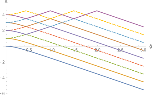
Figure 15: The first several states at $\phi=0$. For each level the dependence of $\Delta$ on the coupling alternates between (5.24) and (5.25) before taking the form (5.24) at large coupling.

At large coupling it is natural to label the states by $n=0,1,2,\dots$ starting from the ground state. However the reshuffling of levels makes it a priori nontrivial to say what is the weak coupling behavior of a state with given $n$. First, we observe that $\Delta$ at zero coupling is given by $L=n/2$ (rounded up). Moreover we found a nice relationship between $n$ and the signs plus or minus in (5.19) determining the 1-loop anomalous dimension. Namely, the levels with $n=0,1,2,\dots$ correspond to the following sequence of signs:

$$--++--++--++\ \dots$$ (5.23)

In order to understand this pattern it is helpful to consider the analytically solvable case when $\phi=0$. We plot the states for this case on Fig. 15. The spectrum of the Schrödinger problem for $\phi=0$ is known exactly Correa:2012nk ,

$$\Delta_{n}=\frac{1}{2}\left[1-\sqrt{16\hat{g}^{2}+1}\right]+n\ ,\ \ n=0,1,2,\dots$$ (5.24)

Here only the values of $n$ for which $\Delta_{n}<0$ actually correspond to bound states. One may try to analytically continue $\Delta_{n}$ in $\hat{g}$ starting from large coupling where it is negative, and arrive to weak coupling. However this would not be correct, as we know that half the levels should have positive slope at weak coupling, corresponding to the choice of the plus sign in the 1-loop correction (5.19). The true levels instead are shown on Fig. 15. At weak coupling half of them are given by an expression of the same form (5.24) but with opposite sign of the square root,

$$\Delta_{m}^{\prime}=\frac{1}{2}\left[1+\sqrt{16\hat{g}^{2}+1}\right]+m\ ,\ \ m=0,1,2,\dots$$ (5.25)

At large coupling the levels are given by (5.24), so dependence on the coupling switches from (5.24) to (5.25) (where $m$ and $n$ may be different) at the point where these two curves intersect. Moreover, at this point two levels meet, and they correspond to adjacent values of $n$ of the same parity. In this way e.g. the levels with even $n$ ‘bounce’ off each other, and the same is true for odd $n$. That explains the pattern of signs in (5.23).

In fact as we see in Fig. 15 the behavior of $\Delta$ can switch multiple times between forms (5.24) and (5.25), before finally becoming the expected curve (5.24) at large coupling. The derivative $\partial\Delta/\partial\hat{g}$ is discontinuous at these switching points. However when $\phi$ becomes nonzero the picture smoothes out and the level crossing at the intersection point is also avoided (though some other level crossings truly remain) as can be see on Fig. 13.

Having $\Delta$ as a piecewise-defined function made up of parts given by (5.24) and (5.25) reminds somewhat the spectrum of local twist-2 operators at zero coupling, where the anomalous dimension becomes a piecewise linear function of the spin (with different regions corresponding e.g. to the BFKL limit bfkl2 ; bfklint or to usual perturbation theory).

One may regard (5.25) as an analytic continuation of (5.24) around the branch point at $\hat{g}=i/4$. There are more branch points at complex values of $\hat{g}$ where curves of the form (5.24) and (5.25) intersect, and we expect all the levels to be obtained from each other by analytic continuation in $\hat{g}$, even for generic $\phi$. Again this situation is reminiscent of the twist operator spectrum.

5.4 Excited states at weak coupling from Feynman diagrams

In this section we compute the diagrams contributing to the anomalous dimensions of the lowest excited states. First let us reproduce the one loop correction to the ground state. For that case there is only one diagram, shown on Fig. 16,

$$D_{0}=\int_{-\Lambda}^{\Lambda}dt\int_{-\Lambda}^{\Lambda}ds\frac{2\hat{g}^{2}}{\cosh(s-t)+\cos(\phi)}\ .$$ (5.26)

It can be computed exactly for any $\Lambda$,

$$D_{0}=\frac{4\hat{g}^{2}}{\sin\phi}\left(2\Lambda\phi-i\text{Li}_{2}\left(-e^{-2\Lambda-i\phi}\right)+i\text{Li}_{2}\left(-e^{i\phi-2\Lambda}\right)+i\text{Li}_{2}\left(-e^{-i\phi}\right)-i\text{Li}_{2}\left(-e^{i\phi}\right)\right)$$ (5.27)

and at large $\Lambda$ it diverges linearly as $D_{0}=8\hat{g}^{2}\frac{\phi}{\sin\phi}\Lambda+{\cal O}(\Lambda^{0})$. Recalling that $\Lambda=\log\frac{x_{12}}{\epsilon}$ we read-off the anomalous dimension $\gamma_{0}=-4\hat{g}^{2}\frac{\phi}{\sin\phi}$ in agreement with (5.3).

For the lowest excited states we have $4$ diagrams (see Fig. 17). For example, the 4th diagram $D_{4}$ is given by the double integral

$$D_{4}=\int_{-\Lambda}^{\Lambda}dt_{1}\int_{t_{1}}^{\Lambda}dt_{2}\,\frac{4\,\hat{g}^{4}}{(\cosh(-\Lambda-t_{1})+\cos\phi)\,(\cosh(\Lambda-t_{2})+\cos\phi)},$$ (5.28)

and corresponds to the following differentiation of the four point function:

$$\partial_{\Lambda_{1}}\partial_{\Lambda_{3}}\left.G(\Lambda_{1},\Lambda_{2},\Lambda_{3},\Lambda_{4})\right|_{\Lambda_{i}=\Lambda}=D_{4}+O(\hat{g}^{6})\ .$$ (5.29)

Below we give the result for these diagrams for large $\Lambda$, keeping $e^{-2\Lambda}$ terms:

$$D_{1} = 4\hat{g}^{2}e^{-2\Lambda}\ ,$$ (5.30)

$$D_{2} = 2\hat{g}^{2}\phi\csc\phi-4\hat{g}^{2}e^{-2\Lambda}+{\cal O}(e^{-4\Lambda})\ ,$$

$$D_{3} = (D_{2})^{2}=4\hat{g}^{4}\phi^{2}\csc^{2}\phi-16\hat{g}^{4}e^{-2\Lambda}\phi\csc\phi+{\cal O}(e^{-4\Lambda})\ ,$$

$$D_{4} = 4\hat{g}^{4}\phi^{2}\csc^{2}\phi+16\hat{g}^{4}e^{-2\Lambda}(-2\Lambda+\phi\cot\phi+\log(\cos\phi+1)-1+\log 2)\ .$$

Combining these diagrams we can construct the operators described in section 5.1, in particular here we consider operators obtained with the insertion of one scalar at the cusp. We have

$$2\,\mathcal{O}_{1}\,\mathcal{\bar{O}}_{1}\left.G(\Lambda_{1},\Lambda_{2},\Lambda_{3},\Lambda_{4})\right|_{\Lambda_{i}=\Lambda}=D_{1}+D_{3}-D_{4}+O(\hat{g}^{6})$$ (5.31)

and from the diagrams computed above we find

$$2\,\mathcal{O}_{1}\,\mathcal{\bar{O}}_{1}\left.G(\Lambda_{1},\Lambda_{2},\Lambda_{3},\Lambda_{4})\right|_{\Lambda_{i}=\Lambda}={4\hat{g}^{2}}e^{-2\Lambda}\left(1+8\hat{g}^{2}\Lambda\right)+\dots$$ (5.32)

Again identifying the cutoff with $\Lambda=\log\frac{x_{12}}{\epsilon}$, we read off the one-loop dimension $\Delta_{1}=1-4\hat{g}^{2}$. Remarkably, it perfectly matches the analytic continuation to weak coupling of the first excited state energy, computed from the QSC above in (5.20). This state corresponds to the second line from below on Fig. 13.

Figure 16: One loop diagram, contributing to the ground state anomalous dimension.

Another operator one can build is obtained from the following combination of derivatives:

$$(\Delta_{0}-\Delta_{2})^{2}\,\mathcal{O}_{2}\,\mathcal{\bar{O}}_{2}\left.G(\Lambda_{1},\Lambda_{2},\Lambda_{3},\Lambda_{4})\right|_{\Lambda_{i}=\Lambda}$$ (5.33)

$$=\left[2\,(\partial_{\Lambda_{1}}\partial_{\Lambda_{3}}+\partial_{\Lambda_{1}}\partial_{\Lambda_{4}})+\Delta_{0}^{2}+4\,\Delta_{0}\,\partial_{\Lambda_{1}}\right]\,\left.G(\Lambda_{1},\Lambda_{2},\Lambda_{3},\Lambda_{4})\right|_{\Lambda_{i}=\Lambda}\ \ \ .$$

The r.h.s. here can be written in terms of the diagrams we have computed and is equal to

$$\gamma_{0}^{2}+4\gamma_{0}\,D_{2}+2(D_{1}+D_{3}+D_{4})+O(\hat{g}^{6})={4\hat{g}^{2}}e^{-2\Lambda}\left(1-8\hat{g}^{2}\Lambda\right)+\dots\ \ ,$$ (5.34)

where $\gamma_{0}=-4\hat{g}^{2}\phi/\sin\phi$ is the one-loop scaling dimension for the ground state. The logarithmic divergence in (5.34) correctly reproduces the energy of the analytic continuation of the second excited state at one loop $\Delta_{2}=1+4\hat{g}^{2}$, matching the QSC result (5.19). This state corresponds to the third line from below in Fig. 13. The one-loop result agrees with the one obtained in Alday:2007he ; Bruser:2018jnc at $\theta=0$ (we expect in the ladders limit this result should be the same).

Figure 17: Four diagrams contributing to the mixing matrix of the cusps with insertions of a scalar operator.

6 Simplifying limit

In this section we consider the limit when $\phi_{1}+\phi_{2}\to\phi_{3}$. Geometrically this limit, which lies at the boundary of the regime of parameters considered in the rest of the paper (4.1), describes the situation where the cusp point $\vec{x}_{3}$ belongs to the circle defined by the extension of the arc $(12)$. In this situation, the points $A$ and $B$ shown in Fig. 7 both coincide with the cusp point $\vec{x}_{3}$. A special case of this limit is the situation when all angles are zero and the triangle reduces to a straight line.

The main simplification comes from the most important part of the result

$$\int_{{\bf|}}\frac{du}{u}q_{1}q_{2}e^{-\phi_{3}u}$$ (6.1)

which now can be evaluated explicitly. When $\phi_{1}+\phi_{2}\to\phi_{3}$ we can deform the integration contour to infinity and notice that only the large $u$ asymptotic of the integrand contributes. This is clear from the following integral

$$\frac{1}{2i\pi}\int_{{\bf|}}{du}\frac{e^{\beta u}}{u^{\alpha}}=\frac{\beta^{\alpha-1}}{\Gamma(\alpha)}\;\;$$ (6.2)

where in our case $\beta=\phi_{1}+\phi_{2}-\phi_{3}$ is small and positive. We see that the integral (6.2) allows us to convert the large $u$ expansion into small $\beta$ series. The large $u$ expansion of the integrand is very easy to deduce from the Baxter equation (2.7), one just has to plug into the Baxter equation (2.7) the ansatz

$$q=e^{\phi u}u^{\Delta}\left(1+\frac{k_{1}}{u}+\frac{k_{2}}{u^{2}}+\dots\right)$$ (6.3)

to get a simple linear system for the coefficients $k_{i}$, which gives

$$k_{1}\sin\phi = \frac{1}{2}(\Delta-1)\Delta\cos\phi-2\hat{g}^{2}$$ (6.4)

$$k_{2}\sin^{2}\phi = \frac{1}{48}(\Delta-2)(\Delta-1)\Delta((3\Delta-1)\cos(2\phi)+3\Delta-5)-(\Delta-1)^{2}\hat{g}^{2}\cos\phi+2\hat{g}^{4},$$ (6.5)

$$\dots$$

which allows us to compute explicitly

$$\int_{{\bf|}}\frac{du}{u}q_{1}q_{2}e^{-\phi_{3}u}=\frac{2i\pi\beta^{-\Delta_{1}-\Delta_{2}}}{\Gamma\left(-\Delta_{1}-\Delta_{2}+1\right)}$$ (6.6)

$$-\frac{i\pi\beta^{-\Delta_{1}-\Delta_{2}+1}\left(-\left(\Delta_{1}-1\right)\Delta_{1}\cot\phi_{1}-\left(\Delta_{2}-1\right)\Delta_{2}\cot\phi_{2}+4\left(g_{1}^{2}\csc\phi_{1}+g_{2}^{2}\csc\phi_{2}\right)\right)}{\Gamma\left(-\Delta_{1}-\Delta_{2}+2\right)}+\dots$$

In this way we get the following small-$\beta$ expansion for the bracket in the numerator of structure constant with insertions at $1$ and $2$:

$${\langle\!\!\langle}q_{1}q_{2}e^{-\phi_{3}u}{\rangle\!\!\rangle} = \frac{1\,}{\Gamma(-\Delta_{1}-\Delta_{2}+1)}$$

$$+ \frac{\left((\Delta_{1}-1)\Delta_{1}\cot\phi_{1}+(\Delta_{2}-1)\Delta_{2}\cot\phi_{2}-4\left(\hat{g}_{1}^{2}\csc\phi_{1}+\hat{g}_{2}^{2}\csc\phi_{2}\right)\right)}{2\,\Gamma(-\Delta_{1}-\Delta_{2}+2)}\,\beta$$

$$+ \dots.$$

In principle, the expansion can be performed to an arbitrary order in $\beta=\phi_{1}+\phi_{2}-\phi_{3}$.

Similarly, the norm factors appearing in the denominator of the structure constants simplify when $\phi_{i}\rightarrow 0$ for one of the cusps $i=1$ or $i=2$. This limit describes the situation where the cusp angle disappears. As we reviewed in Sec. 5.3, at $\phi=0$ the Schrödinger equation becomes exactly solvable and the spectrum is explicitly known Correa:2012nk .

The main ingredient for the computation of the norm is the integral (3.38), and it is clear that for small $\phi$ it simplifies for the very same mechanism we have just described. In particular, every term in the $1/u$ expansion of the integrand gives an integral of the kind (6.2), which allow us to organize the result in powers of $\phi$. Naturally we should also take into account the scaling of the coefficients $k_{i}$ appearing in (6.3) for $\phi\sim 0$. Notice that the expressions (6.5) are apparently singular at $\phi\sim 0$. However, a nice feature of this limit is that most of these divergences are cancelled systematically due to the fact that the scaling dimension too depends on $\phi$ in a nontrivial way. In particular, we found numerically that, for the QSC solution corresponding to the ground state, the coefficients $k_{n}$ have the following scaling for $\phi\rightarrow 0$:

$$\left\{k_{1},k_{2},k_{3},k_{4},k_{5},\dots\right\}\sim\left\{0\,,\,O(1)\,,\,0\,,\,O(1)\,,\,0\,,\,O(1)\,,\dots\right\}.$$ (6.8)

This observation is quite powerful. Indeed, combined with the parametric form of the coefficients (6.5), the requirement that they scale as (6.8) fixes all terms in the expansion of $\Delta$ for small $\phi$ !

More precisely, we find that the scaling (6.8) corresponds to two solutions for $\Delta(\phi)$: one is the ground state, for which we reproduce the results of Correa:2012nk obtained using perturbation theory of the Schrödinger equation, namely, for the first two orders,

$$\Delta_{0} = \frac{1}{2}\left(1-\sqrt{1+16\,\hat{g}^{2}}\right)+\frac{\hat{g}^{2}\left(-16\hat{g}^{2}+\sqrt{16\hat{g}^{2}+1}+1\right)}{\left(16\hat{g}^{2}-3\right)\sqrt{16\hat{g}^{2}+1}}\,\phi^{2}+\dots.$$ (6.9)

The other solution describes one of the excited states trajectories

$$\Delta_{0}^{\prime}=\frac{1}{2}\left(1+\sqrt{16\hat{g}^{2}+1}\right)+\frac{\hat{g}^{2}\left(16\hat{g}^{2}+\sqrt{16\hat{g}^{2}+1}-1\right)}{\left(16\hat{g}^{2}-3\right)\sqrt{16\hat{g}^{2}+1}}\,\phi^{2}+\dots$$ (6.10)

It is straightforward to generate higher orders in $\phi$ with this method. The remaining infinitely many states can be described allowing for a more general scaling of the coefficients $k_{m}$, see Appendix D for details and some results.

Plugging in the scaling of coefficients (6.8), for the solution corresponding to the ground state we find

$${\langle\!\!\langle}q^{2}{\rangle\!\!\rangle}=\frac{1}{\Gamma(1-2\Delta)}+O(\phi^{2}),$$ (6.11)

which combined with (6) gives a finite result for the OPE coefficient at $\phi_{1}=\phi_{2}=\phi_{3}=0$:

$$\left.C^{\bullet\bullet\circ}_{123}\right|_{\phi_{i}=0}=\left.\frac{\sqrt{\Gamma(1-2\Delta_{1})\,\Gamma(1-2\Delta_{2})}}{\Gamma(1-\Delta_{1}-\Delta_{2})}\right|_{\phi_{i}=0}=\frac{\sqrt{\Gamma\left(\sqrt{16\hat{g}_{1}^{2}+1}\right)}\sqrt{\Gamma\left(\sqrt{16\hat{g}_{2}^{2}+1}\right)}}{\Gamma\left(\frac{1}{2}\left(\sqrt{16\hat{g}_{1}^{2}+1}+\sqrt{16\hat{g}_{2}^{2}+1}\right)\right)},$$ (6.12)

where we used (6.9) in the last step. This is in perfect agreement with the result of Kim:2017sju . It is simple to obtain further orders in a small angle expansion, the next-to leading order in all angles is reported in Appendix D.

7 Numerical evaluation

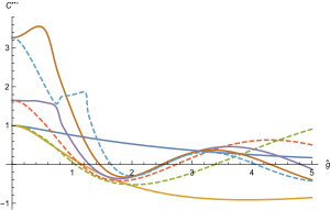
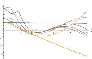
Figure 18: Diagonal HHL correlator for several first excited states ($n=0,1,\dots,7$) with all angles equal to $\phi=1$ (left) or $\phi=1/3$ (right). Colors are the same as on Figure 13.

The expression for the 3-cusp correlator we found has the form of an integral $\int_{{\bf|}}q_{\Delta_{1}}q_{\Delta_{2}}e^{-u\phi_{3}}\frac{du}{2\pi iu}$ which is guaranteed to converge for large enough coupling as the q-functions behave as $e^{\phi u}u^{\Delta}$ where $\Delta$ decreases linearly with $\hat{g}$ and reaches arbitrarily large negative values. However, we would like to be able to use these expressions at small coupling too, where the convergence of the integral is only guaranteed when both states are ground states, but for the excited states the integral is formally not defined.

To define the integrals we introduce the following $\zeta$-type of regularization. We multiply the integrand by some negative power $u^{\alpha}$, compute the integral for large negative enough $\alpha$ and then analytically continue it to zero value. The key integral is (6.2) where the r.h.s. gives the ananlytic continuation to all values of $\alpha$.

We see that for large negative $\alpha$ the expression decays factorially. This fact is crucial for our numerical evaluation of the correlation function. Once the value of the energy is known numerically it is very easy to get an asymptotic expansion of the q-functions at large $u$ to essentially any order. However, since the poles of the q-functions accumulate at infinity, this expansion is doomed to have zero convergence radios. Nevertheless if we expand the integrand at large $u$ and then integrate each term of the expansion using (6.2) we enhance the convergence of this series by a factorially decaying factor making it a very efficient tool for the numerical evaluation.

We applied this method to compute the correlation function for several excited states (see Fig. 18). The method allows one to compute the correlator even faster than the spectrum. We checked that it works very well for $\phi\sim 1$ giving $10$ digits precision easily, but seems to diverge for $\phi=1.5$. To cross check our precision we also used the $d\Delta/dg$ correlator (2.17), which is given by the same type of integrals.

8 Correlation functions at weak coupling

In this section we present some explicit results for the structure constants at weak coupling.

Our all-loop expression for the structure constants (1.3) is rather straightforward to evaluate perturbatively. First one should find the Q-function $q$ at weak coupling, which can be done by iteratively solving the Baxter equation as discussed in section 5.3. The result at each order is given as a linear combination of twisted $\eta$-functions (see (5.15)) multiplied by exponentials $e^{\phi u}$ and rational functions of $u$, as in e.g. (5.18). Then the integrals appearing in the numerator and denominator of (1.3) can be easily done by closing the integration contour to encircle the poles of $q(u)$ in the lower half-plane, giving an infinite sum of residues:

$$\frac{1}{2\pi i}\,\int_{{\bf|}}f(u)\,du=\sum_{n=0}^{\infty}\left.\text{Res}\,f(u)\right|_{u=-in}.$$ (8.1)

The residues come from poles of the $\eta$-functions, e.g.

$$\eta^{z}_{n}=\frac{z^{m}}{(u+im)^{n}}+O(1),\;\;\;u\to-im,\;\;\;m=0,1,\dots,$$ (8.2)

To get the residue one may need more coefficients of this Laurent expansion, which are given by zeta values or polylogarithms. Finally one should take the infinite sum in (8.1) which again may give polylogs.

In this way we have computed the first 1-2 orders of the weak coupling expansions, as a demonstration (going to higher orders is in principle straightforward, limited by computer time and the need to simplify the resulting multiple polylogarithms). The integrals giving the norm of $q$-functions are especially simple. Below, we assume that $q(u)$ is normalized such that the leading coefficient in the large $u$ expansion is $1$, so $q(u)\simeq u^{\Delta}\,e^{\phi u}$. For the ground state ($L=0$) we find

$${\langle\!\!\langle}q^{2}{\rangle\!\!\rangle}_{L=0}=1+8\,\hat{g}^{2}\,\frac{\phi}{\sin\phi}\,\gamma_{\text{E}}+\mathcal{O}(\hat{g}^{4}),$$ (8.3)

where $\gamma_{\text{E}}$ is the Euler-Mascheroni constant. For the excited states $(L,\pm)$ corresponding to insertion of $L$ scalars, we have

$${\langle\!\!\langle}q^{2}{\rangle\!\!\rangle}_{1,\pm} = \pm 8\hat{g}^{2}+\dots$$ (8.4)

$${\langle\!\!\langle}q^{2}{\rangle\!\!\rangle}_{2,\pm} = \pm 16\,\cos\phi\;\hat{g}^{2}+\dots$$ (8.5)

The $L=3$ result is given in (C.5). Notice here that for the states $2^{+}$ and $2^{-}$ the signs of ${\langle\!\!\langle}q^{2}{\rangle\!\!\rangle}$ are different at weak and strong coupling. Indeed, at strong coupling the relation with the wavefunctions (3.38) implies that ${\langle\!\!\langle}q^{2}{\rangle\!\!\rangle}$ is positive/negative for even/odd states, respectively. Since the even state is $2^{-}$ (see Table 1), in (8.5) we see explicitly that these signs can change at weak coupling.

The structure constants are more involved. For the HHL correlator without scalar insertions we have to 1-loop order

$$(C^{\bullet\bullet\circ})_{L=0}=1+\hat{g}_{1}^{2}F_{123}+\hat{g}_{2}^{2}F_{213}+\dots$$ (8.6)

where

$$F_{123}= \frac{1}{\sin\phi_{1}}\left[2i\left(\text{Li}_{2}(e^{-2i\phi_{1}})-\text{Li}_{2}(e^{-i\phi_{1}-i\phi_{2}+i\phi_{3}})+\text{Li}_{2}(e^{i\phi_{1}-i\phi_{2}+i\phi_{3}})\right)-\frac{i\pi^{2}}{3}\right.$$

$$\left.+2\left(\phi_{1}-\phi_{2}+\phi_{3}\right)\log\left(\frac{1-e^{-i\phi_{1}-i\phi_{2}+i\phi_{3}}}{1-e^{i\phi_{1}-i\phi_{2}+i\phi_{3}}}\right)-4\phi_{1}\log\left(\frac{\sin\frac{1}{2}\left(\phi_{1}+\phi_{2}-\phi_{3}\right)}{\sin\phi_{1}}\right)\right]\ .$$

For the correlators with excited states both the numerator and the denominator in the expression (1.3) for $C^{\bullet\bullet o}$ vanish at weak coupling. Due to this even the leading order in the expansion is nontrivial and requires using $q(u)$ computed to $\hat{g}^{2}$ accuracy. For the correlators with two $L=1$ states we find

$$(C^{\bullet\bullet\circ})_{L=1} = \frac{1}{2}\,\left(\frac{\hat{g}_{1}}{\hat{g}_{2}}\pm\frac{\hat{g}_{2}}{\hat{g}_{1}}\right)+\dots\ ,$$ (8.8)

while for $L=2$ we get a nontrivial dependence on the angles,

$$(C^{\bullet\bullet\circ})_{L=2}= \frac{1}{2}\,\left(\sqrt{\frac{\hat{g}_{1}^{2}\,\cos\phi_{1}}{\hat{g}_{2}^{2}\,\cos\phi_{2}}}\pm\sqrt{\frac{\hat{g}_{2}^{2}\,\cos\phi_{2}}{\hat{g}_{1}^{2}\,\cos\phi_{1}}}\right)$$

$$\times\left(-\frac{\cos\phi_{3}}{\sin\phi_{1}\,\sin\phi_{2}}+\cot\phi_{1}\,\cot\phi_{2}+2\right)+\dots\ \ .$$

Here we have the plus sign for correlators corresponding to $(L^{+},L^{+})$ or $(L^{-},L^{-})$ states, and the minus sign for the $(L^{+},L^{-})$ correlator.

Curiously, the HHL results do not have a smooth limit when one of the couplings goes to zero corresponding to the HLL case (this is related to a singularity in the 2-pt function normalization). This means we have to compute the HLL correlators separately. For H_nLL with the excited state being $\Delta_{1,+}$ we get

$$(C^{\bullet\circ\circ})_{1^{+},0,0}=-\sqrt{2\,\hat{g}^{2}}\,\frac{\cos(\frac{1}{2}(\phi_{2}-\phi_{3}))}{\cos{\frac{1}{2}\phi_{1}}}\ \ ,$$ (8.10)

while for $\Delta_{1,-}$ we have

$$(C^{\bullet\circ\circ})_{1^{-},0,0}=-\sqrt{2\,\hat{g}^{2}}\,\frac{\sin(\frac{1}{2}(\phi_{2}-\phi_{3}))}{\sin{\frac{1}{2}\phi_{1}}}\ \ .$$ (8.11)

For the $L=2$ states we find

$$(C^{\bullet\circ\circ})_{2^{+},0,0} = -\hat{g}\,i\,\frac{\sin(\phi_{2}-\phi_{3})}{\sin{\phi_{1}}}\,\sqrt{\cos\phi_{1}}\ \ ,$$ (8.12)

$$(C^{\bullet\circ\circ})_{2^{-},0,0} = \hat{g}\,i\,\frac{\sqrt{\cos\phi_{1}}}{\sin^{2}\phi_{1}}\,(\cos\phi_{1}\,\cos(\phi_{2}-\phi_{3})-1)\ \ .$$ (8.13)

These two structure constants are purely imaginary due to the sign of ${\langle\!\!\langle}q^{2}{\rangle\!\!\rangle}$ at weak coupling. We also present the results for the $L=3$ states in Appendix C.

9 The 4-point function and twisted OPE

In this section we examine more closely the expression for the 4-point function which we obtained in (5.1). We interpret it as an OPE expansion and cross-test it at weak coupling against our perturbative data for the correlation functions. We also present some conjectures on the generalization of this OPE expansion and its applications to the computation of more general correlators.

9.1 The 4-cusp correlation function

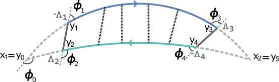
Figure 19: The 4-cusp correlator. Its OPE-like expansion (9.1) provides predictions for the HLL structure constants.

Our starting point is an OPE-like formula (5.1) for the 4-cusp correlator. It is based on the 2-pt function of cusps with angle $\phi_{0}$, but the four cutoffs $\Lambda_{1},\dots,\Lambda_{4}$ give it the structure of a 4-point function with four cusp angles $\phi_{a}$ determined by $\Lambda$’s as shown on Fig. 19. To make the analogy more clear we notice that we can get rid of the wavefunctions in (5.1) entirely and rewrite it in terms of the structure constants as follows

$$G(\Lambda_{1},\Lambda_{2},\Lambda_{3},\Lambda_{4})=\sum_{n=0}^{\infty} {C_{012}^{\bullet_{n}\circ\circ}}{C^{\bullet_{n}\circ\circ}_{043}}{}\left(\frac{e^{-2\Lambda}}{L_{043}L_{012}}\right)^{\Delta_{n}}\;,$$ (9.1)

where $\Lambda\equiv\frac{\Lambda_{1}+\Lambda_{2}+\Lambda_{3}+\Lambda_{4}}{4}$, while the angles $\phi_{1},\dots,\phi_{4}$ at the cusps $y_{a}$ (see Fig. 19) can be found from $w_{\phi_{0}}(\Lambda_{a}-\Lambda_{b})=\phi_{b}-\phi_{a}$ with $w$ defined by (3.29). More explicitly,

$$e^{-i\phi_{12}}=\frac{e^{\Lambda_{12}}+e^{i\phi_{0}}}{1+e^{\Lambda_{12}+i\phi_{0}}}\;\;,\;\;e^{-i\phi_{43}}=\frac{e^{\Lambda_{43}}+e^{i\phi_{0}}}{1+e^{\Lambda_{43}+i\phi_{0}}}\;,$$ (9.2)

where we denoted $\phi_{ab}=\phi_{a}-\phi_{b}$ and

$$\Lambda_{12}=\Lambda_{1}-\Lambda_{2},\ \ \Lambda_{43}=\Lambda_{4}-\Lambda_{3}\ .$$ (9.3)

The factor $L_{abc}$ as before is defined by

$$L_{abc}=\frac{\sqrt{\sin\frac{1}{2}(\phi_{a}+\phi_{b}-\phi_{c})\,\sin\frac{1}{2}(\phi_{a}-\phi_{b}+\phi_{c})}}{\sin\phi_{a}}.$$ (9.4)

We can view equation (9.1) as defining the 4-cusp correlator in terms of the structure constants, opening an easy way for computing this quantity in various regimes including numerically at finite coupling. This equation suggests a natural interpretation in terms of an OPE expansion for pairs of cusps. To understand this point, let us first investigate the space-time dependence of the 4pt function (9.1), which comes through the factors

$$\left(\frac{e^{-2\Lambda}}{L_{012}\,L_{034}}\right)^{\Delta_{n}}.$$ (9.5)

To decode the dependence of (9.5) on the cusp positions, it is convenient to introduce six complex parameters: four space-time positions $y_{i}$, $i=1,\dots,4$, defined as

$$y_{1}=\zeta_{+}(-\Lambda_{1}),\;\;\;y_{2}=\zeta_{-}(\Lambda_{2}),\;\;\;y_{3}=\zeta_{+}(\Lambda_{3}),\;\;\;y_{4}=\zeta_{-}(-\Lambda_{4}),$$ (9.6)

(where $\zeta_{\pm}$ is the parameterization defined by (3.4)) together with the intersection points of the two arcs $x_{1}$, $x_{2}$ (see Fig. 19), which we denote as $y_{0}\equiv x_{1}$, $y_{5}\equiv x_{2}$. These six points are not all independent as we can express $y_{5}$ in terms of the other five complex coordinates through the solution of the equations

$$\frac{y_{53}\,y_{10}}{y_{31}\,y_{50}}=\frac{y_{53}^{*}\,y_{10}^{*}}{y_{31}^{*}\,y_{50}^{*}},\;\;\;\;\;\frac{y_{54}\,y_{20}}{y_{42}\,y_{50}}=\frac{y_{54}^{*}\,y_{20}^{*}}{y_{42}^{*}\,y_{50}^{*}},$$ (9.7)

where $y_{ab}=y_{a}-y_{b}$. From these two relations we can obtain $y_{5}$ as a rational function of $y_{i}$, $i=0,\dots,4$ and their complex conjugates.

Eliminating the parameters $\Lambda_{i}$ in favour of the $y_{i}$ coordinates, we find that the term (9.5) appearing in the 4pt function can be written as

$$\left(\frac{e^{-2\Lambda}}{L_{012}\,L_{034}}\right)^{\Delta_{n}}=|y_{05}^{2}|^{\Delta_{n}}\,\frac{|y_{12}|^{\Delta_{n}}}{|y_{15}\,y_{25}\,|^{\Delta_{n}}}\,\frac{|y_{34}|^{\Delta_{n}}}{|y_{30}\,y_{40}\,|^{\Delta_{n}}}.$$ (9.8)

Notice that this is the space-time dependence of the product of two 3pt functions, divided by a 2pt function, and (9.1) can be rewritten suggestively as

$$G=\sum_{n}\frac{C_{512}^{\bullet_{n}\circ\circ}}{|y_{15}\,y_{25}\,|^{\Delta_{n}}\,|y_{12}|^{-\Delta_{n}}}\,\frac{C_{043}^{\bullet_{n}\circ\circ}}{|y_{30}\,y_{40}\,|^{\Delta_{n}}\,|y_{34}|^{-\Delta_{n}}}\,\left(\frac{1}{|y_{05}|^{2\Delta_{n}}}\right)^{-1}.$$ (9.9)

This relation is illustrated in Fig. 20 and it strongly reminds the usual OPE decomposition of a 4pt function in terms of 3pt correlators. In the next subsection we provide an interpretation of this relation on the operator level.

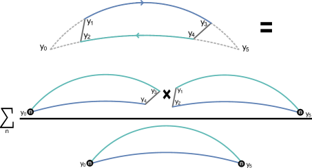
Figure 20: The OPE decomposition of the four-point function, illustrating equation (9.9).

9.2 The cusp OPE

Let us now rederive the decomposition (9.9) of the 4pt function from first principles using the logic inspired by the usual OPE. The idea, illustrated in Fig. 21, is to express the cusps at $y_{1}$, $y_{2}$ as a combination of cusp operators inserted at $y_{0}$:

$$W_{y_{1}}^{y_{3}}\,W_{y_{2}}^{y_{4}}=\sum_{n}\,\mathcal{C}^{y_{1},y_{2}}_{n}\;\left[\mathcal{O}_{n}\,\left(W_{y_{4}}^{y_{0}}\,W_{y_{0}}^{y_{3}}\right)\right],$$ (9.10)

where $\mathcal{C}^{y_{1},y_{2}}_{n}$ are some coefficients, $W_{x}^{y}$ are the Wilson line operators defined in (3.2), and $\mathcal{O}_{n}$ represent projector operators on the $n$-th excitation of the cusp at $y_{0}$. To make sense of the rhs of (9.10), we need to specify a regularization scheme; we assume that the $\epsilon$ regularization defined in the rest of the paper is used, and the projectors $\mathcal{O}_{n}$ are the ones defined explicitly in section 5.1. Notice that the expansion corresponds to a change in the limit of integration of the Wilson lines. Derivatives of the Wilson line with respect to its endpoints produce the scalar insertions described in Sec. 5.1. For this reason, at least in the ladder limit considered here, we expect that only these excitations are involved in the OPE. To determine the coefficients $\mathcal{C}_{n}^{y_{1},y_{2}}$, we proceed in the standard logic of the OPE and place equation (9.10) inside an expectation value. Considering the limit where $y_{3}$,$y_{4}$ converge towards $y_{5}$ (with the usual point-splitting regulator $\epsilon$), and projecting on the $n$-th state, we have

$$\bar{\mathcal{O}}_{n}\langle W_{y_{1}}^{y_{5}}\,W_{y_{2}}^{y_{5}}\rangle=\mathcal{N}_{\Delta_{n},\epsilon}\,\frac{C_{512}^{\bullet_{n}\circ\circ}}{|y_{15}\,y_{25}|^{\Delta_{n}}\,|y_{12}|^{-\Delta_{n}}},$$ (9.11)

where we noticed that in this limit the configuration reduces to an HLL 3pt function, which we related to the structure constant as in Sec. 5.2. Here, the constant $\mathcal{N}_{\Delta_{n},\epsilon}$ is the square root of the normalization of the 2pt function, explicitly defined in (5.9). On the other hand from the rhs of (9.10) we obtain (see Fig. 22):

$$\bar{\mathcal{O}}_{n}\,\left(\sum_{m}\,\mathcal{O}_{m}\;\langle\,W_{y_{0}}^{y_{5}}\;W_{y_{0}}^{y_{5}}\,\rangle\right)=\mathcal{C}_{n}^{y_{1},y_{2}}\,\frac{\mathcal{N}_{\Delta_{n},\epsilon}^{2}}{|y_{05}|^{2\Delta_{n}}},$$ (9.12)

therefore we find the coefficients:

$$\mathcal{C}_{n}^{y_{1},y_{2}}=C_{512}^{\bullet_{n}\circ\circ}\,\left(\frac{|y_{12}\,y_{05}^{2}|}{|y_{15}\,y_{25}|}\right)^{\Delta_{n}}\,\mathcal{N}_{\Delta_{n},\epsilon}^{-1}.$$ (9.13)

Taking the expectation value of (9.10) now fixes the 4pt function precisely to the form (9.9).

In the next subsection we will discuss how to apply similar logic to higher-point correlators.

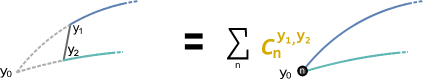
Figure 21: Expansion of the Wilson lines starting at points $y_{1}$, $y_{2}$ in terms of Wilson arcs emanating from $y_{0}$, as written in equation (9.10).

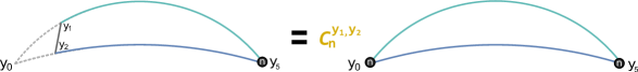
Figure 22: Graphical representation of equation (9.12) determining the value of $\mathcal{C}_{n}^{y_{1},y_{2}}$.

9.3 OPE expansion of more general correlators

The OPE approach we presented above can also be applied to more general correlation functions. As one of the possible generalizations, let us consider the four point function shown in Figure 23. For simplicity of notation, we assume that the same scalar polarization $\vec{n}$ is chosen for the Wilson lines denoted as $C$ and $B$, while on lines $A$ and $D$ we have a different polarization vector $\vec{m}$. This defines a configuration where the two cusps at $y_{1}$ and $y_{4}$ are not protected, while the remaining two are. Explicitly, we are considering the expectation value:

$$G_{1243}^{\bullet\circ\bullet\circ}=\frac{\langle W_{y_{1}}^{y_{2}}(\vec{m})\;W_{y_{2}}^{y_{4}}(\vec{m})\;W_{y_{4}}^{y_{3}}(\vec{n})\;W_{y_{3}}^{y_{1}}(\vec{n})\;\rangle}{\mathcal{N}_{1}\,\mathcal{N}_{4}},$$ (9.14)

where we divided by the usual 2pt function normalization factors $\mathcal{N}_{1}$, $\mathcal{N}_{4}$ for the unprotected cusps (defined explicitly in (5.9)) in order to get a finite result.

Our conjecture for this quantity is based on the assumption that we can use the same type of OPE expansion as in the previous section. This allows us to replace each pair of consecutive cusps with a sum over excitations of a single cusp, whose position is defined by the geometry. For instance, the two cusps at $y_{3}$ and $y_{4}$, which are defined by the consecutive sides $A$ $B$ $C$ of the Wilson loop, are traded for a sum over excitations of a single cusp at the point $D$, defined by the extension of the lines $A$ and $C$.

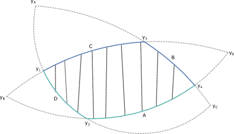
Figure 23: The 4pt function $G_{1243}^{\bullet\circ\bullet\circ}$ of two protected and two unprotected cusps. We assume that only two scalar polarizations are involved: $\vec{n}$ on the arcs $B$,$C$ and $\vec{m}$ on the arcs $A$,$D$, so that the configuration depends on a single effective coupling.

As expected, the OPE expansion gives rise to nontrivial crossing equations. Let us see this explicitly here. Taking into account the space-time dependence as in the previous section, from the contraction of $y_{3}$ and $y_{4}$ we obtain (see Fig. 24 on the right):

$$G_{1243}^{\bullet\circ\bullet\circ}=\sum_{n}\,\frac{C_{D12}^{\bullet_{n}\bullet\circ}}{|y_{1D}|^{\Delta_{n}+\Delta_{0}}\,|y_{2D}|^{\Delta_{n}-\Delta_{0}}\,|y_{12}|^{\Delta_{0}-\Delta_{n}}}\,\frac{C_{B43}^{\bullet_{n}\bullet\circ}}{|y_{B4}|^{\Delta_{n}+\Delta_{0}}\,|y_{B3}|^{\Delta_{n}-\Delta_{0}}\,|y_{34}|^{\Delta_{0}-\Delta_{n}}}\,|y_{BD}|^{2\Delta_{n}},$$ (9.15)

which now involves HHL structure constants. Performing the OPE decomposition in the crossed channel, which corresponds to contracting $y_{1}$ and $y_{3}$ (see Fig. 24 on the left), yields a different expansion:

$$G_{1243}^{\bullet\circ\bullet\circ}=\sum_{n}\,\frac{C_{A42}^{\bullet_{n}\bullet\circ}}{|y_{4A}|^{\Delta_{n}+\Delta_{0}}\,|y_{2A}|^{\Delta_{n}-\Delta_{0}}\,|y_{24}|^{\Delta_{0}-\Delta_{n}}}\,\frac{C_{C13}^{\bullet_{n}\bullet\circ}}{|y_{C1}|^{\Delta_{n}+\Delta_{0}}\,|y_{C3}|^{\Delta_{n}-\Delta_{0}}\,|y_{13}|^{\Delta_{0}-\Delta_{n}}}\,|y_{AC}|^{2\Delta_{n}}.$$ (9.16)

Notice that we left the dependence on all angles implicit; however, we point out that the sums in (9.15) and (9.16) are over different spectra, characterized by the same coupling but different cusp angles. Proving the equivalence between (9.15) and (9.16) would be an important test of these expressions, and more generally of the OPE expansion on which they are based. We leave this nontrivial task for the future. Crossing relations such as the one presented above could perhaps also be used to gain information on the HHH structure constants, which would appear in one of the two channels in the OPE expansion of correlators of the form $G_{1234}^{\bullet\bullet\circ\circ}$.

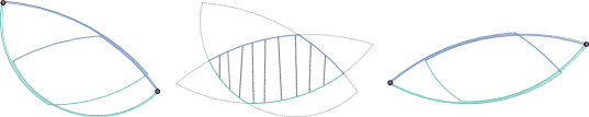
Figure 24: The two alternative OPE decompositions of the 4pt function $G_{1243}^{\bullet\circ\bullet\circ}$.

9.4 Checks at weak coupling

In this section, we present some tests of the 4pt OPE expansion (9.9) at weak coupling. We will show that perturbative expansion of the 4pt function reproduces our results for HLL structure constants. In Appendix G.2 we also verify at 1 loop that when two of the four points collide, the 4pt function reduces precisely to a 3pt HLL correlator, including the expected spacetime dependence. This provides an important test of our results for the structure constants and also of the OPE expression for the 4pt function.

At one loop it is very easy to compute the 4pt function, and we find

$$G(\Lambda_{1},\Lambda_{2},\Lambda_{3},\Lambda_{4})=1+\int_{-\Lambda_{4}}^{\Lambda_{2}}ds\int_{-\Lambda_{1}}^{\Lambda_{3}}dt\frac{2\hat{g}^{2}}{\cosh(s+t)+\cos(\phi_{0})}\ ,$$ (9.17)

resulting in

$$G = 1+\frac{2i\hat{g}^{2}}{\sin\phi_{0}}\Big{[}\text{Li}_{2}\left(-e^{-i\phi_{0}+\Lambda_{12}}\right)-\text{Li}_{2}\left(-e^{i\phi_{0}+\Lambda_{12}}\right)-\text{Li}_{2}\left(-e^{-i\phi_{0}-\Lambda_{23}}\right)+\text{Li}_{2}\left(-e^{i\phi_{0}-\Lambda_{23}}\right)$$ (9.18)

$$- \text{Li}_{2}\left(-e^{-i\phi_{0}+\Lambda_{14}}\right)+\text{Li}_{2}\left(-e^{i\phi_{0}+\Lambda_{14}}\right)+\text{Li}_{2}\left(-e^{-i\phi_{0}+\Lambda_{43}}\right)-\text{Li}_{2}\left(-e^{i\phi_{0}+\Lambda_{43}}\right)\Big{]}\ ,$$

where we denoted (note the difference with (9.3))

$$\Lambda_{23}=\Lambda_{2}+\Lambda_{3},\ \ \Lambda_{14}=\Lambda_{1}+\Lambda_{4}\ .$$ (9.19)

Expanding this expression at large $\Lambda$ we get:

$$G = g_{0}+\Lambda h_{0}+e^{-2\Lambda}g_{1}+e^{-4\Lambda}g_{2}+e^{-6\Lambda}g_{3}+{\cal O}(e^{-8\Lambda})\ ,$$ (9.20)

where the first coefficient is rather involved,

$$g_{0} = 2\frac{\hat{g}^{2}}{\sin\phi_{0}}\left(i\text{Li}_{2}\left(-e^{\Lambda_{12}-i\phi_{0}}\right)-i\text{Li}_{2}\left(-e^{i\phi_{0}+\Lambda_{12}}\right)+i\text{Li}_{2}\left(-e^{\Lambda_{43}-i\phi_{0}}\right)-i\text{Li}_{2}\left(-e^{i\phi_{0}+\Lambda_{43}}\right)\right)$$ (9.21)

$$+ 2\,{\hat{g}^{2}}{}\frac{\Lambda_{12}\phi_{0}+\Lambda_{43}\phi_{0}}{\sin\phi_{0}}+1\ ,$$

while the rest are simpler,

$$h_{0} = 8\frac{\hat{g}^{2}\phi_{0}}{\sin\phi_{0}}\ ,\ \ \ \ \ \ \ \ \ \ \ \ \ \ \ \ \ \ \ \ \ \ \ \ \ \ \ \ \ \ \ \ \ \ g_{1}=8\hat{g}^{2}\cosh\left(\frac{\Lambda_{12}+\Lambda_{43}}{2}\right)\ ,$$ (9.22)

$$g_{2} = -4\hat{g}^{2}\cosh\left(\Lambda_{12}+\Lambda_{43}\right)\cos(\phi_{0})\ ,\ \ \ \ \ g_{3}=\frac{8\hat{g}^{2}}{9}\cosh\left(\frac{3(\Lambda_{12}+\Lambda_{43})}{2}\right)(2\cos(2\phi_{0})+1)\ .$$

Rewriting this in terms of the angles using (9.2) we obtain

$$L_{012}L_{043}\;g_{1}=2\hat{g}^{2}\left(\frac{\cos\frac{\phi_{12}}{2}\cos\frac{\phi_{43}}{2}}{\cos^{2}\frac{\phi_{0}}{2}}+\frac{\sin\frac{\phi_{12}}{2}\sin\frac{\phi_{43}}{2}}{\sin^{2}\frac{\phi_{0}}{2}}\right)=C^{\bullet_{1}\circ\circ}_{012}C^{\bullet_{1}\circ\circ}_{043}+C^{\bullet_{2}\circ\circ}_{012}C^{\bullet_{2}\circ\circ}_{043}\ ,$$ (9.23)

where we used that there are only two states $n=1,2$ which converge to $\Delta=1$ at weak coupling. Furthermore, we can identify precisely $n=1$ and $n=2$, by using the fact that the $n=1$ state is associated with an odd state and thus should give an odd function in $\phi_{12}$. This results in

$$C^{\bullet_{1}\circ\circ}_{012}=\pm\sqrt{2\hat{g}^{2}}\frac{\sin\frac{\phi_{12}}{2}}{\sin\frac{\phi_{0}}{2}}\;\;,\;\;C^{\bullet_{2}\circ\circ}_{012}=\pm\sqrt{2\hat{g}^{2}}\frac{\cos\frac{\phi_{12}}{2}}{\cos\frac{\phi_{0}}{2}}\ ,$$ (9.24)

in complete agreement with our perturbative results (8.11) and (8.10) ! In the same way we find for the $L=2$ states

$$C^{\bullet_{3}\circ\circ}_{012} = \pm i\hat{g}\frac{\sin\phi_{12}}{\sin\phi_{0}}\sqrt{\cos\phi_{0}}\ ,$$ (9.25)

$$C^{\bullet_{4}\circ\circ}_{012} = \pm i\hat{g}\frac{\sqrt{\cos\phi_{0}}}{\sin^{2}\phi_{0}}\left(\cos\phi_{0}\cos\phi_{12}-1\right)\ ,$$ (9.26)

in agreement with (8.13) and (8.12). We also verified the $L=3$ states and reproduced expressions (C), (C) given in Appendix C.

We also notice that the term $h_{0}$ is indeed equal to $2\Delta_{0}^{(1)}$ i.e. the ground state energy at 1 loop. Finally, the expression $g_{0}$ can be compared with the HLL structure constant of three ground states, which reads at weak coupling

$$(C^{\bullet oo})_{L=0}=1+\hat{g}^{2}F_{123}+\dots$$ (9.27)

where $F_{123}$ is given explicitly by the lengthy formula (8). From the OPE (9.1) we expect that

$$g_{0}=1+\hat{g}^{2}\,\left(-\Delta_{0}^{(1)}\,\log{(L_{043}\,L_{012})}+F_{012}+F_{043}\right)\ ,$$ (9.28)

and indeed our result (9.21) for $g_{0}$ precisely matches this complicated expression! This is a nontrivial check of the OPE as well as the HLL structure constant at 1 loop.

10 Conclusions

Our main result is the all-loop computation of the expectation value of a Wilson line with three cusps with particular class of insertions at the cusps in the ladders limit. We demonstrated that in terms of the q-functions it takes a very simple form, reminiscent of the SoV scalar product. The key ingredient in the construction is the bracket ${\langle\!\!\langle}\cdot{\rangle\!\!\rangle}$, which allows to wrote the result in a very compact form (1.3). We also found a similar representation for the diagonal correlator of two cusps and the Lagrangian (1.5). This gives a clear indication that the Quantum Spectral Curve and the SoV approach can be able to provide an all-loop description of 3-point correlators.

In order to generalise our results one could consider correlators with more complicated insertions which should help to reveal more generally the structure of the SoV-type scalar product. We expect in this case that the bracket ${\langle\!\!\langle}\cdot{\rangle\!\!\rangle}$ will involve product of several Q-functions:

$${\langle\!\!\langle}q_{1}q_{2}{\rangle\!\!\rangle}=\int\mu(u_{1},\dots,u_{L})q_{1}(u_{1})\dots q_{1}(u_{L})q_{2}(u_{1})\dots q_{2}(u_{L})du_{1}\dots du_{L}$$ (10.1)

for some universal measure function $\mu$, which should not depend on the states, but could be a non-trivial function of coupling. It would also be important to extend the results obtained in this paper to the more general HHH configuration where all three effective couplings are nonzero. The form of our result (1.3), where the BPS cusp always appears with a different sign for the rapidity, suggests that in the most general case one of the Q-functions may need to be treated on a different footing as the other two. Therefore, the generalization to the HHH case may be nontrivial and reveal new important elements.

Going away from the ladders limit (see e.g. Bykov:2012sc ; Henn:2012qz ) could also give some hints about the measure in the complete ${\cal N}=4$ SYM theory and eventually lead to the solution of the planar theory. Potentially a simpler problem is the fishnet theory Gurdogan:2015csr ; Gromov:2017cja ; Grabner:2017pgm , where some $3-$ and $4-$point correlators were found explicitly and have a very similar form to the $\phi\to 0$ limit of our correlator. As they involve only conventional local operators this is another natural setting for further developing our approach. It would be also interesting to consider the cusp in ABJM theory for which the ladders limit was recently elucidated in Bonini:2016fnc . It would be also useful to utilize the perturbative data from other approaches Escobedo:2010xs ; Gromov:2012uv ; Caetano:2014gwa ; Basso:2015zoa ; Basso:2017muf ; Eden:2016xvg ; Fleury:2016ykk in order to guess the measure factor.

Let us mention that our result incorporates all finite size corrections (in particular the 2-point functions are given exclusively by wrapping contributions). These corrections are rather nontrivial to deal with in the hexagon Basso:2015zoa approach to computation of correlators (see also Eden:2016xvg ; Fleury:2016ykk ; Bargheer:2017nne ; Eden:2017ozn ). The diagonal correlators, which we studied numerically in this paper at any value of coupling, are proven to be particularly hard in the hexagon formulation which is known to be incomplete in this situation. Nevertheless, it would be interesting to draw parallels between the two approaches. The hexagon techniques could be especially helpful in generalisation of our results for the longer states, where the wrapping corrections are suppressed by powers of ‘t Hooft coupling.

Another possible limit which would be interesting to consider is near-BPS. This could be either the small spin limit of twist-2 local operators or the $\phi\simeq\theta$ limit of the cusps. In both cases the analytic solutions of the QSC are known explicitly Gromov:2013qga ; Gromov:2014bva (see also Gromov:2012eu ), which could be helpful in fixing the measure factor. In particular, at the leading order, the Q-functions $q(u)$ describing the excited states of a cusp are orthogonal on $[-2g,2g]$ with the measure $\mu(u)=\sinh(2\pi u)$ Gromov:2012eu ; Gromov:2013qga ; Sizov:2013joa . It is not clear how this measure is related to our result yet, but there are some promising signs which we discuss in the Appendix F. Let us point out that the naive guess that this is the measure we need is not consistent in an obvious way with the structure expected from SoV (10.1), where we expect multiple interactions for the insertions of such scalars. It would be really interesting to compare with localisation methods, which are applicable in the near-BPS limit. Some preliminary results were reported recently Giombi:2018qox (see also Bonini:2015fng for partial results for the spectrum). Let us also mention that often the measure can be bootstrapped from the orthogonality requirement, see Nsl2 for a higher-loop result in the $sl(2)$ sector. One could try this strategy too in order to find the measure in ${\cal N}=4$ SYM.

As another new result, we understood the meaning of the bound states of the Schrödinger problem resulting from Bethe-Salpeter resummation of ladder diagrams. They correspond to insertion of scalar operators of the same type as those on the Wilson lines, see Klebanov:2006jj for a string theory interpretation. From the point of view of the Bethe-Salpeter equation the excited states can be interpreted as resonances – poles of the resolvent on the non-physical sheet, which can be reached by analytic continuation under the branch cut of the continuum. As such they are hard to study analytically or numerically. In the QSC approach there is no continuum spectrum and the bound states can be studied on completely equal footing with the vacuum state. Moreover they can be easily tracked away from the ladders limit and should still correspond to scalar insertions. In addition, we showed that our results for the 3-cusp correlators immediately generalize to the case with these scalar insertions.

Our result opens the way to efficiently study the cusp with scalar insertions at arbitrary values of $\theta$ using the powerful QSC methods, both analytically and numerically. We already found the first few orders in the weak and strong coupling expansions of the energies of excited states in the ladders limit. The result at $1$ loop for the first excited state matches the known 1-loop prediction Alday:2007he (assuming it is not changed in the ladders limit).

It would be also important to further investigate the OPE picture we presented in section 9. In order to reveal more structure for higher point correlators it would be very useful to find a compact way to perform the spectral sums appearing in the OPE. Recent results of Gross:2017aos for the SYK model suggest that this could be feasible at least in the ladder limit. One could also explore the applicability of modern conformal bootstrap techniques Rattazzi:2008pe ; ElShowk:2012ht for the OPE expansion we considered. Finally, the structure of our OPE expansion is very reminiscent of the one for null polygonal Wilson loops Alday:2010ku , and it could be useful to explore this analogy.

Appendix A Technical details on the QSC

Here we provide details concerning the formulation of the QSC for the cusp anomalous dimension at generic values of the coupling $g$ and the angles $\phi,\theta$ Gromov:2015dfa .

The ${\bf P}$-functions of the QSC can be written in a compact form as

$${\bf P}_{1}(u) = +\epsilon\;u^{1/2}\;e^{+\theta u}\;{\bf f}(+u)\ ,$$ (A.1)

$${\bf P}_{2}(u) = -\epsilon\;u^{1/2}\;e^{-\theta u}\;{\bf f}(-u)\ ,$$

$${\bf P}_{3}(u) = +\epsilon\;u^{1/2}\;e^{+\theta u}\;{\bf g}(+u)\ ,$$

$${\bf P}_{4}(u) = +\epsilon\;u^{1/2}\;e^{-\theta u}\;{\bf g}(-u)\ .$$

where the functions ${\bf f}(u)$ and ${\bf g}(u)$ have powerlike asymptotics at large $u$ with ${\bf f}\simeq 1/u$ and ${\bf g}\simeq u$. The prefactor $\epsilon$ in this normalization reads

$$\epsilon=\sqrt{\frac{i}{2}}\;\frac{\cos\theta-\cos\phi}{\sin\theta}\;.$$ (A.2)

The functions ${\bf f}(u)$ and ${\bf g}(u)$ are regular outside of the cut $[-2g,2g]$, which can be resolved using the Zhukovsky variable $x(u)$,

$$x(u)=\frac{u+\sqrt{u-2g}\sqrt{u+2g}}{2g}\;\;,\;\;u=(x+1/x)g\;$$ (A.3)

where we choose the solution with $|x|>1$. In terms of $x$ these functions simply become power series,

$${\bf f}(u)=\frac{1}{gx}+\sum_{n=1}^{\infty}\frac{g^{n-1}A_{n}}{x^{n+1}}\;\;,\;\;{\bf g}(u)=\frac{u^{2}+B_{0}u}{gx}+\sum_{n=1}^{\infty}\frac{g^{n-1}B_{n}}{x^{n+1}}\;.$$ (A.4)

The coefficients $A_{n}$ and $B_{n}$ encode nontrivial information about the AdS conserved charges including $\Delta$. In particular, for the first few of them we have

$$A_{1}g^{2}-B_{0} = -\frac{2\cos\theta\cos\phi+\cos(2\theta)-3}{2\sin\theta(\cos\theta-\cos\phi)}\;,$$ (A.5)

$$\Delta^{2} = \frac{(\cos\theta-\cos\phi)^{3}}{\sin\theta\sin^{2}\phi}\left[A_{3}g^{6}+\frac{A_{1}^{2}g^{4}(1-\cos\theta\cos\phi)}{\sin\theta(\cos\theta-\cos\phi)}-A_{2}g^{4}\cot\theta\right.$$ (A.6)

$$\left.-g^{2}\left(B_{0}+B_{1}+\cot\theta\right)-A_{1}g^{2}\left(A_{2}g^{4}-2g^{2}+\frac{1}{\sin^{2}\theta}\right)\right]\;.$$

The fourth order Baxter type equation (2) on ${\bf Q}_{i}$ is written in terms of several determinants involving the ${\bf P}$-functions. They are given by:

$$D_{0} = {\rm det}\left(\begin{array}[]{llll}{\bf P}^{1[+2]}&{\bf P}^{2[+2]}&{\bf P}^{3[+2]}&{\bf P}^{4[+2]}\\ {\bf P}^{1}&{\bf P}^{2}&{\bf P}^{3}&{\bf P}^{4}\\ {\bf P}^{1[-2]}&{\bf P}^{2[-2]}&{\bf P}^{3[-2]}&{\bf P}^{4[-2]}\\ {\bf P}^{1[-4]}&{\bf P}^{2[-4]}&{\bf P}^{3[-4]}&{\bf P}^{4[-4]}\end{array}\right)\;,$$ (A.11)

$$D_{1} = {\rm det}\left(\begin{array}[]{llll}{\bf P}^{1[+4]}&{\bf P}^{2[+4]}&{\bf P}^{3[+4]}&{\bf P}^{4[+4]}\\ {\bf P}^{1}&{\bf P}^{2}&{\bf P}^{3}&{\bf P}^{4}\\ {\bf P}^{1[-2]}&{\bf P}^{2[-2]}&{\bf P}^{3[-2]}&{\bf P}^{4[-2]}\\ {\bf P}^{1[-4]}&{\bf P}^{2[-4]}&{\bf P}^{3[-4]}&{\bf P}^{4[-4]}\end{array}\right)\;,$$ (A.16)

$$D_{2} = {\rm det}\left(\begin{array}[]{llll}{\bf P}^{1[+4]}&{\bf P}^{2[+4]}&{\bf P}^{3[+4]}&{\bf P}^{4[+4]}\\ {\bf P}^{1[+2]}&{\bf P}^{2[+2]}&{\bf P}^{3[+2]}&{\bf P}^{4[+2]}\\ {\bf P}^{1[-2]}&{\bf P}^{2[-2]}&{\bf P}^{3[-2]}&{\bf P}^{4[-2]}\\ {\bf P}^{1[-4]}&{\bf P}^{2[-4]}&{\bf P}^{3[-4]}&{\bf P}^{4[-4]}\end{array}\right)\;,$$ (A.21)

$$\bar{D}_{1} = {\rm det}\left(\begin{array}[]{llll}{\bf P}^{1[-4]}&{\bf P}^{2[-4]}&{\bf P}^{3[-4]}&{\bf P}^{4[-4]}\\ {\bf P}^{1}&{\bf P}^{2}&{\bf P}^{3}&{\bf P}^{4}\\ {\bf P}^{1[+2]}&{\bf P}^{2[+2]}&{\bf P}^{3[+2]}&{\bf P}^{4[+2]}\\ {\bf P}^{1[+4]}&{\bf P}^{2[+4]}&{\bf P}^{3[+4]}&{\bf P}^{4[+4]}\end{array}\right)\;,$$ (A.26)

$$\bar{D}_{0} = {\rm det}\left(\begin{array}[]{llll}{\bf P}^{1[-2]}&{\bf P}^{2[-2]}&{\bf P}^{3[-2]}&{\bf P}^{4[-2]}\\ {\bf P}^{1}&{\bf P}^{2}&{\bf P}^{3}&{\bf P}^{4}\\ {\bf P}^{1[+2]}&{\bf P}^{2[+2]}&{\bf P}^{3[+2]}&{\bf P}^{4[+2]}\\ {\bf P}^{1[+4]}&{\bf P}^{2[+4]}&{\bf P}^{3[+4]}&{\bf P}^{4[+4]}\end{array}\right)\;.$$ (A.31)

A.1 Derivation of the quantization condition

Let us explain the derivation of (2.9) in detail. For consistency with standard QSC notation Gromov:2015dfa we denote in this section the two solutions of the Baxter equation (2.7) as $q_{1}$ and $q_{4}$ which in the notation of section 2.1 corresponds to

$$q_{+}=q_{1},\ \ \ q_{-}=q_{4}\ \ ,$$ (A.32)

with large $u$ asymptotics $q_{1}\sim e^{u\phi}u^{\Delta},\ \ q_{4}\sim e^{-u\phi}u^{-\Delta}$.

First we notice that the Baxter equation (2.7) is invariant under complex conjugation, so $\bar{q}_{1}$ and $\bar{q}_{4}$ are linear combination of the two solutions $q_{1}$ and $q_{4}$ with $i$-periodic coefficients that we denote $\Omega_{i}^{j}$,

$$\bar{q}_{1} = \Omega_{1}^{1}q_{1}+\Omega_{1}^{4}q_{4}$$ (A.33)

$$\bar{q}_{4} = \Omega_{4}^{1}q_{1}+\Omega_{4}^{4}q_{4}\ .$$ (A.34)

Our strategy is to constrain as much as possible the form of $\Omega$’s and then fix them completely using the gluing conditions from the QSC.

The analytic properties of $q$’s already impose strong restrictions on $\Omega_{i}^{j}$. Both $q_{1}(u)$ and $q_{4}(u)$ are analytic in the upper half-plane, but the Baxter equation implies that they can have second order poles at $u=-in,\;n=1,2,\dots$ in the lower half-plane. Accordingly, $\bar{q}_{1},\bar{q}_{4}$ will have second order poles in the upper half plane which can only originate from $\Omega$’s in the r.h.s.​ of (A.33) and (A.34). Therefore these $\Omega$’s can have at most 2nd order poles. Their rate of growth at $u\to+\infty$ and $u\to-\infty$ is moreover constrained by the known asymptotics of $q_{1},q_{4}$. To fix normalization we impose for $u\to+\infty$

$$q_{1}\sim e^{u\phi}u^{\Delta},\ \ \ q_{4}\sim\frac{i}{8t^{4}\Delta\sin^{2}\phi}e^{-u\phi}u^{-\Delta}$$ (A.35)

where the constant prefactor for $q_{4}$ is determined by the canonical normalisation of Q-functions). Assuming $\phi>0$ we see that $q_{1}$ is the dominant solution at $u\to+\infty$ and therefore e.g. $\Omega_{4}^{1}$ must vanish for large positive $u$ (though not necessarily for $u\to-\infty)$. By arguments of this type we can write all the components of $\Omega$ in terms of just a few parameters, namely

$$\bar{q}_{1} = q_{1}\left(\frac{a_{1}}{(e^{2\pi u}-1)^{2}}+\frac{a_{2}}{e^{2\pi u}-1}+1\right)+q_{4}\left(\frac{a_{3}}{(e^{2\pi u}-1)^{2}}+\frac{a_{4}}{e^{2\pi u}-1}-a_{3}+a_{4}\right)$$ (A.36)

$$\bar{q}_{4} = q_{1}\left(\frac{b_{1}}{(e^{2\pi u}-1)^{2}}+\frac{b_{2}}{e^{2\pi u}-1}\right)+q_{4}\left(\frac{b_{3}}{(e^{2\pi u}-1)^{2}}+\frac{b_{4}}{e^{2\pi u}-1}-1\right)$$ (A.37)

Moreover, we can use the trick suggested in Gromov:2017cja to express these parameters $a_{n},b_{n}$ in terms of $q$’s. As in Gromov:2016rrp we will focus on $\Omega_{1}^{4}$, which as we see from (A.36) is given by

$$\Omega_{1}^{4}=\frac{a_{3}}{(e^{2\pi u}-1)^{2}}+\frac{a_{4}}{e^{2\pi u}-1}-a_{3}+a_{4}\ \ .$$ (A.38)

Shifting $u\to u+i$ in (A.33), (A.34) and using $i$-periodicity of $\Omega$ we find

$$\bar{q}_{1}(u+i) = \Omega_{1}^{1}(u)q_{1}(u+i)+\Omega_{1}^{4}(u)q_{4}(u+i)$$ (A.39)

$$\bar{q}_{4}(u+i) = \Omega_{4}^{1}(u)q_{1}(u+i)+\Omega_{4}^{4}(u)q_{4}(u+i)\ .$$ (A.40)

Now we can view the four equations (A.33), (A.34), (A.39), (A.40) as a linear system on the four components of $\Omega$. Solving it we can we find $\Omega_{1}^{4}$,

$$\Omega_{1}^{4}=\frac{q_{1}(u+i)\bar{q}_{1}(u)-q_{1}(u)\bar{q}_{1}(u+i)}{q_{1}(u+i)q_{4}(u)-q_{1}(u)q_{4}(u+i)}\ \ .$$ (A.41)

Nicely, the denominator of (A.41) is precisely the Wronskian of the Baxter equation, which is a constant we denote by $C_{W}$. Its precise value is not important here but can be found from the asymptotics (A.35),

$$C_{W}\equiv q_{1}(u+i)q_{4}(u)-q_{1}(u)q_{4}(u+i)=-{\Delta t^{4}\sin\phi}\ .$$ (A.42)

Thus we have

$$\Omega_{1}^{4}(u)=\frac{1}{C_{W}}\left[q_{1}(u+i)\bar{q}_{1}(u)-q_{1}(u)\bar{q}_{1}(u+i)\right]\ .$$ (A.43)

We expect that $\Omega_{1}^{4}$ has a singularity at $u=0$, which in this expression can only come from $\bar{q}_{1}(u+i)$. Using the fact that $\bar{q}_{1}$ satisfies the original Baxter equation (2.7), we find

$$\bar{q}_{1}(u+i)=-\frac{4\hat{g}^{2}\bar{q}_{1}(0)}{u^{2}}-\frac{4\hat{g}^{2}\bar{q}_{1}^{\prime}(0)+2\Delta\bar{q}_{1}(0)\sin\phi}{u}+\mathcal{O}(1),\ \ u\to 0$$ (A.44)

Plugging this into (A.43) gives

$$\Omega_{1}^{4}=\frac{4\hat{g}^{2}q_{1}(0)\bar{q}_{1}(0)}{C_{W}u^{2}}+\frac{4\hat{g}^{2}\left(\bar{q}_{1}(0)q_{1}^{\prime}(0)+q_{1}(0)\bar{q}_{1}^{\prime}(0)\right)+2\Delta q_{1}(0)\bar{q}_{1}(0)\sin\phi}{C_{W}u}+\mathcal{O}(1),\ \ u\to 0$$ (A.45)

At the same time, expanding the expression for $\Omega_{1}^{4}$ from (A.38) we find

$$\Omega_{1}^{4}=\frac{a_{3}}{4\pi^{2}u^{2}}+\frac{a_{4}-a_{3}}{2\pi u}+\mathcal{O}(1),\ \ u\to 0$$ (A.46)

Comparing (A.45) with (A.46) we can express $a_{3}$ and $a_{4}$ in terms of $q_{1}(0)$ and $q_{1}^{\prime}(0)$, in particular

$$a_{3}-a_{4}=-\frac{4\pi\left[2\hat{g}^{2}\left(\bar{q}_{1}(0)q_{1}^{\prime}(0)+q_{1}(0)\bar{q}_{1}^{\prime}(0)\right)+\Delta q_{1}(0)\bar{q}_{1}(0)\sin\phi\right]}{C_{W}}\ \ .$$ (A.47)

So far we have not used any relations from the QSC involving analytic continuation around the branch points. Now we will apply one of such relations, which was derived in Gromov:2016rrp using the gluing condition for $\tilde{q}_{1}$ given in (2.3). It reads

$$\tilde{\Omega}_{1}^{4}-\Omega_{1}^{4} = u\bar{q}_{1}(u)q_{1}(u)-u\bar{q}_{1}(-u)q_{1}(-u)\ \ .$$ (A.48)

In fact we will only use that as a consequence of this relation $\Omega_{1}^{4}$ must be even, which gives

$$a_{3}=a_{4}\ ,\ \ \ \ \Omega_{1}^{4}=\frac{a_{3}}{4\sinh^{2}\pi u}\ \ .$$ (A.49)

Combining the first relation with (A.47) we get precisely the quantization condition (2.9) presented above.

A.2 Quantization condition from asymptotics of the $\Omega$ functions

There is also an alternative way to arrive at the quantization condition, which though just an observation at the moment is very instructive for the discussion that will follow in section 3. In this alternative approach we start from the same Baxter equation (2.7) but never use any relations from the QSC involving tilde, i.e. analytic continuation around the branch points such as in (2.3). Instead we observed that it is sufficient to demand that $\Omega_{1}^{4}$ vanishes at $u\to+\infty$. This immediately fixes $a_{3}=a_{4}$ and thus leads via (A.47) (which as we showed above follows from the Baxter equation) to the same quantization condition (2.9). The importance of this observation will become apparent in section 3, where we will see that the vanishing asymptotics of $\Omega_{1}^{4}$ ensures finiteness of various scalar products that play a key role in our construction.

Curiously, in the fishnet theory Gurdogan:2015csr ; Grabner:2017pgm it is also possible to derive the quantization condition solely from asymptotics of $\Omega$ as was recently found in Grtoapp . It would be interesting to better understand the underlying reason behind this.

Appendix B Quantization condition and square-integrability of the wave function

In Sec. 3.3, we introduced an explicit map between the Q-function and a solution of the stationary Schrödinger equation:

$$\frac{F(z)}{2\pi}=\,e^{-\Delta z/2}\int_{{\bf|}}\,q(u)\,e^{w_{\phi}(z)\,u}\,\frac{du}{2\pi iu}.$$ (B.1)

As we showed there, the fact that $q(u)$ satisfies the Baxter equation implies that $F(z)$ solves the Schrödinger equation. This statement does not require that the quantization conditions are satisfied, and is valid for any value of the parameter $\Delta$. In this Appendix we show that, for $\Delta<0$, the quantization conditions are equivalent to the square-integrability of $F(z)$. In particular, notice that, since the potential in the Schrödinger equation is vanishing at infinity, any solution to (3.27) can have one of the two behaviours $\sim e^{\pm\Delta z/2}$ at large $z$, therefore it can either decay or grow exponentially. We will show that $F(z)$ is always decaying at $z\rightarrow+\infty$, while it is decaying at $z\rightarrow-\infty$ if and only if $q(u)$ satisfies the quantization conditions.

We will use the same convention as in Sec. A and denote the two independent solution of the Baxter equation as $q_{1}$ and $q_{4}$, see (A.32), where $q(u)=q_{1}(u)$.

They are characterized by the following asymptotics in the upper half plane

$$q_{1}(u)\sim e^{\phi u}\,u^{\Delta},\;\;\;\;\;q_{4}(u)\sim e^{-\phi u}\,u^{-\Delta}.$$ (B.2)

In preparation for the following argument, we will need to determine the asymptotics of $q_{1}(u)$ also along the part of the integration contour in (B.1) which extends in the lower half plane. To determine the asymptotics along this line, we reflect it to the upper half plane using complex conjugation, and then use the exact relation (A.36) between $q$ and $\bar{q}$. This leads to

$$(q(c-is))^{*} = \bar{q}(c+is)=\Omega_{1}^{1}(c+is)\,q_{1}(c+is)+\Omega_{1}^{4}(c+is)\,q_{4}(c+is)\simeq\Omega_{1}^{4}(c+is)\,q_{4}(c+is)$$

$$\sim e^{-\phi\,(c+is)}\,(c+is)^{-\Delta}\,\left(a_{4}-a_{3}+\frac{a_{4}}{e^{2\pi(c+is)}-1}+\frac{a_{3}}{\left(e^{2\pi(c+is)}-1\right)^{2}}\right),$$

where the constants $a_{3}$, $a_{4}$ are defined in (A.38). Notice that in (LABEL:eq:qexpl) we dropped the terms proportional to $\Omega_{1}^{1}$, since they give a subdominant contribution suppressed as $\sim u^{\Delta}$ (in this appendix we assume $\Delta<0$ throughout). Equation (LABEL:eq:qexpl) shows that $q(u)$ grows for large $|\text{Im}(u)|$ in the lower half plane. Despite this fact, notice that the integral (3.28) still converges as long as $-1<\Delta<0$, since, for any finite $z$, the integrand is oscillatory.

Let us now come to the core of the argument. To determine the behaviour of $F(z)$ for $z\rightarrow+\infty$, we study the following limit

$$\lim_{z\rightarrow+\infty}e^{\frac{\Delta z}{2}}\,F(z),\;\;\;(\Delta<0),$$ (B.4)

which vanishes if and only if $F(z)$ is a decaying solution of the Schrödinger equation. From (3.28), we find

$$\lim_{z\rightarrow+\infty}e^{\frac{\Delta z}{2}}\,F(z)=\lim_{z\rightarrow+\infty}\int_{{\bf|}}\,\frac{q(u)\,e^{-\phi u}}{u}\,e^{+2\sin\phi\,e^{-z}u}\,du=\int_{{\bf|}}\,\frac{q(u)\,e^{-\phi u}}{u}\,du=0,$$ (B.5)

where the last term in (B.5) is zero due to the fact that the integrand is suppressed at least as $\sim u^{\Delta-1}$ at large $u$. Therefore, we found that $F(z)$ is always decaying for $z\rightarrow\infty$.

To analyse the situation at $z\sim-\infty$ we now look at the limit

$$\lim_{z\rightarrow-\infty}e^{-\frac{\Delta z}{2}}\,F(z) = \lim_{z\rightarrow-\infty}-i\,\left(\int_{{\bf|}}\,\frac{q(u)}{u}\,e^{+\phi u}\,e^{-2\sin\phi e^{z}\,u}du\right)$$ (B.6)

$$= \int_{{\bf|}}\,\frac{q(u)}{u}\,e^{+\phi u}\,du.$$ (B.7)

Notice that by definition this limit is finite if and only if $F(z)$ is decaying at $z\sim-\infty$. Accordingly, we find that, for a generic value of $\Delta$, the last integral in (B.7) is not convergent. To understand why, notice that, as a consequence of (LABEL:eq:qexpl), the integrand in (B.7) behaves as

$$\frac{q(u)\,e^{\phi u}}{u}\sim(a_{3}-a_{4})\,u^{-1-\Delta},\;\;\;\;u\sim-i\infty$$ (B.8)

along the part of the contour extending in the lower-half plane. Therefore, the integral is clearly divergent.

However, the quantization conditions coming from the QSC correspond precisely to $a_{3}=a_{4}$ (see (A.47) )! When they are satisfied, the most singular part of the asymptotics (B.8) is cancelled and the integral (B.7) is still convergent, which implies that $F(z)$ is a square-integrable function. Therefore we have just shown that the (negative) scaling dimensions described by the QSC are associated with the spectrum of bound states of the Schrödinger equation (3.27). While we derived this relation for $\Delta$ in a specified range $-1<\Delta<0$, this correspondence can be extended beyond this regime by analytic continuation in the coupling constant. This analytic continuation is such that, for small enough coupling, $\Delta_{n}$ becomes positive for almost all levels except for the ground state. In this regime, the scaling dimensions no longer correspond to bound states in terms of the Schrödinger potential problem, but can be understood as resonances.

Appendix C Perturbative results

Here we list our weak coupling results supplementing the main text.

First we present The perturbative results for $\Delta$ corresponding to the excited states with $L=2,3$, complementing the result for $L=1$ given in (5.20):

$$\Delta_{2,-} = 2-2\frac{\sin 2\phi}{\sin\phi}\hat{g}^{2}+(-8\cos^{2}\phi+16\phi\cos^{2}\phi\cot\phi+8)\hat{g}^{4}+\dots$$ (C.1)

$$\Delta_{2,+} = 2+2\frac{\sin 2\phi}{\sin\phi}\hat{g}^{2}+(-8\cos^{2}\phi-16\phi\sin\phi\cos\phi-8)\hat{g}^{4}+\dots$$ (C.2)

$$\Delta_{3,-} = 3-\frac{4\sin 3\phi}{3\sin\phi}\hat{g}^{2}$$

$$+\left[\frac{16}{9}\phi(2\cos\phi-1)^{3}(2\cos\phi+1)\cot\frac{\phi}{2}-\frac{16}{27}\left((2\cos 2\phi+1)^{2}-18\cos\phi\right)\right]\hat{g}^{4}+\dots$$

$$\Delta_{3,+} = 3+\frac{4\sin 3\phi}{3\sin\phi}\hat{g}^{2}$$

$$+\left[-\frac{16}{9}\phi(2\cos\phi-1)(2\cos\phi+1)^{3}\tan\frac{\phi}{2}-\frac{16}{27}\left((2\cos 2\phi+1)^{2}+18\cos\phi\right)\right]\hat{g}^{4}+\dots$$

For the $L=3^{\pm}$ excited states we also have

$${\langle\!\!\langle}q^{2}{\rangle\!\!\rangle}=\pm 32\,\hat{g}^{2}\,(2\cos(2\phi)+1)+\dots\ \ \ .$$ (C.5)

Now let us present further results for the structure constants. For the HLL correlator with the $3^{+}$ state we have to leading order in the coupling

$$\left.C^{\bullet\circ\circ}\right|_{3^{+},0,0} = \frac{\hat{g}}{6}\;\left(\cos(2\phi_{1})+\frac{1}{2}\right)^{\frac{1}{2}}\,\csc\left(\frac{\phi_{1}}{2}\right)\cot(\phi_{1})\sec^{2}\left(\frac{\phi_{1}}{2}\right)\cos\left(\frac{\phi_{2}-\phi_{3}}{2}\right)$$

$$\times ((\sec(\phi_{1})+2)\cos(\phi_{2}-\phi_{3})-2\sec(\phi_{1})-1)+\dots$$

and for the $3^{-}$ state:

$$\left.C^{\bullet\circ\circ}\right|_{3^{-},0,0} = -\frac{\hat{g}}{6}\;\left(\cos(2\phi_{1})+\frac{1}{2}\right)^{\frac{1}{2}}\,\,\csc^{2}\left({\frac{\phi_{1}}{2}}\right)\csc({\phi_{1}})\,\sec\left({\frac{\phi_{1}}{2}}\right)\,\sin\left({\frac{\phi_{2}-\phi_{3}}{2}}\right)$$

$$\times \left((2\cos({\phi_{1}})-1)\,\cos(\phi_{2}-\phi_{3})+\cos({\phi_{1}})-2\right)+\dots$$

For the HHL structure constant with $(3^{+},3^{+})$ or $(3^{-},3^{-})$ states we find at leading order

$$(C^{\bullet\bullet\circ})_{3^{\pm},3^{\pm}} = \frac{\cot(\phi_{2})\csc(2\phi_{2})\cot(\phi_{1})\csc(2\phi_{1})\,\left(2\hat{g}_{2}^{2}\cos(2\phi_{2})+\hat{g}_{2}^{2}+2\hat{g}_{1}^{2}\cos(2\phi_{1})+\hat{g}_{1}^{2}\right)}{4\,\hat{g}_{2}\,\hat{g}_{1}\,\sqrt{2\cos(2\phi_{2})+1}\sqrt{2\cos(2\phi)+1}}$$

$$\times {\Big{(}}12\cos\phi_{3}\,(3\sin\phi_{1}\sin\phi_{2}+\cos\phi_{1}\cos\phi_{2})-10\cos(2(\phi_{1}-\phi_{2}))$$

$$-\cos(2(\phi_{1}+\phi_{2}))+8\cos(2\phi_{1})+8\cos(2\phi_{2})-3\cos(2\phi_{3})-14{\Big{)}}$$

$$+ \dots$$

Appendix D Results for the small-$\phi$ expansion

At $\phi=0$ the spectrum and resonances are described by the following trajectories

$$\Delta_{n,{\phi=0}}=\frac{1}{2}\,\left((2n+1)-\sqrt{1+16\,\hat{g}^{2}}\right),\;\;\;\;\Delta_{n,\phi=0}^{\prime}=\frac{1}{2}\,\left((2n+1)+\sqrt{1+16\,\hat{g}^{2}}\right),$$ (D.1)

for $n=0,1,2,3,\dots$. Inspecting the numerical solution of the QSC equations for a few states, we observe a clear pattern in the scaling of the coefficients in the large-$u$ expansion (6.3) for small $\phi$. For a state converging to one of the trajectories $\Delta=\Delta_{n,{\phi=0}}+O(\phi)^{2}$ or $\Delta=\Delta_{n,{\phi=0}}^{\prime}+O(\phi^{2})$, the coefficients scale as follows as $\phi\sim 0$: for even $n$,

$$\left\{k_{1},k_{2},k_{3},k_{4},\dots\right\}\sim\left\{\phi,\,1,\,\phi,\,1,\,\phi,\,1,\dots\right\}\,\phi^{-n},\;\;\;n=0,2,4,6,\dots,$$ (D.2)

while for odd $n$:

$$\left\{k_{1},k_{2},k_{3},k_{4},\dots\right\}\sim\left\{\,1,\,\phi,\,1,\,\phi,\,1,\,\phi,\,1,\dots\right\}\,\phi^{-n},\;\;\;n=1,3,5,7,\dots.$$ (D.3)

Notice that this means that the large-$u$ expansion becomes approximately even or odd for even or odd $n$, respectively. Imposing the validity of a given scaling behaviour such as (D.2) or (D.3) generates all terms in the small-$\phi$ expansion of $\Delta$.

In particular, from the inspection of a few trajectories we conjecture a general formula for the expansion up to order $\phi^{2}$:

$$\Delta=\frac{1}{2}\left((2n+1)\pm\sqrt{16\hat{g}^{2}+1}\right)\pm\frac{\hat{g}^{2}\left(16\hat{g}^{2}\pm(2n+1)\,\sqrt{16\hat{g}^{2}+1}+(2n(n+1)-1)\right)}{\left(16\hat{g}^{2}-3\right)\sqrt{16\hat{g}^{2}+1}}\,\phi^{2}+\dots.$$ (D.4)

We cross-checked this result at finite $\phi$ but large $g$ in section (E). Higher orders in $\phi$ are straightforward to obtain, even though the expressions become cumbersome. We report the result only for the ground state:

$$\Delta_{0} = \frac{1}{2}\left(1-\sqrt{1+16\,\hat{g}^{2}}\right)+\frac{\hat{g}^{2}\left(-16\hat{g}^{2}+\sqrt{16\hat{g}^{2}+1}+1\right)}{\left(16\hat{g}^{2}-3\right)\sqrt{16\hat{g}^{2}+1}}\,\phi^{2}+$$ (D.5)

$$+ \left(-\frac{(\tau-1)(\tau+1)^{2}\left(5\tau^{5}+40\tau^{4}+97\tau^{3}+68\tau^{2}+18\tau+24\right)}{768\tau^{3}(\tau+2)^{3}(\tau+4)}\right)\,\phi^{4}+\dots,$$ (D.6)

where we set $\tau=\sqrt{1+16\,\hat{g}^{2}}$.

As explained in Sec. 6, one can also obtain a systematic expansion of the structure constants in the limit where $\phi_{1}\sim\phi_{2}\sim\phi_{3}\sim 0$. In the case where the ground state is inserted at every cusp we obtain, up to next-to-leading order:

$$\frac{C^{\bullet\bullet\circ}_{123}}{\left.C^{\bullet\bullet\circ}_{123}\right|_{\phi_{1}=\phi_{2}=\phi_{3}=0}}=1-2(\phi_{1}+\phi_{2}-\phi_{3})\,\left(\frac{\left(\hat{g}_{1}^{2}\phi_{1}+\hat{g}_{2}^{2}\phi_{2}\right)}{\sqrt{16\hat{g}_{1}^{2}+1}+\sqrt{16\hat{g}_{2}^{2}+1}}\right)$$

$$+ \phi_{1}^{2}\,\left(\frac{\hat{g}_{1}^{2}\left(-48\hat{g}_{1}^{2}+\sqrt{16\hat{g}_{1}^{2}+1}-2\left(-16\hat{g}_{1}^{2}+\sqrt{16\hat{g}_{1}^{2}+1}+1\right)\psi^{(0)}\left(\sqrt{16\hat{g}_{1}^{2}+1}\right)+7\right)}{2\left(16\hat{g}_{1}^{2}-3\right)\sqrt{16\hat{g}_{1}^{2}+1}}\right)$$

$$+ \phi_{2}^{2}\,\left(\frac{\hat{g}_{2}^{2}\left(-48\hat{g}_{2}^{2}+\sqrt{16\hat{g}_{2}^{2}+1}-2\left(-16\hat{g}_{2}^{2}+\sqrt{16\hat{g}_{2}^{2}+1}+1\right)\psi^{(0)}\left(\sqrt{16\hat{g}_{2}^{2}+1}\right)+7\right)}{2\left(16\hat{g}_{2}^{2}-3\right)\sqrt{16\hat{g}_{2}^{2}+1}}\right),$$

where $\psi^{(0)}(z)=\Gamma^{\prime}(z)/\Gamma(z)$ and $\left.C^{\bullet\bullet\circ}_{123}\right|_{\phi_{1}=\phi_{2}=\phi_{3}=0}$ is given in (6.12).

For the norm of excited states at small $\phi$ we get , in proximity of the trajectories (D.1),

$${\langle\!\!\langle}q^{2}_{\Delta_{n,\phi=0}}{\rangle\!\!\rangle} = \frac{(-1)^{n}\,(n!)}{\Gamma(1+n-2\,\Delta_{n,\phi=0})}+\dots=\frac{(-1)^{n}\,(n!)}{\Gamma(-n+\sqrt{1+16\,\hat{g}^{2}})}+\dots,$$ (D.8)

$${\langle\!\!\langle}q^{2}_{\Delta^{\prime}_{n,\phi=0}}{\rangle\!\!\rangle} = \frac{(-1)^{n}\,(n!)}{\Gamma(1+n-2\,\Delta^{\prime}_{n,\phi=0})}+\dots=\frac{(-1)^{n}\,(n!)}{\Gamma(-n-\sqrt{1+16\,\hat{g}^{2}})}+\dots$$ (D.9)

In the case of excited states, the small-angles limit for the numerator of structure constants depends on the relative scaling of the three angles. For example, for the HHL structure constants involving two $n=1$ trajectories, assuming $\phi_{3}=0$ and $\phi_{1}=\phi_{2}=\phi\sim 0$ small, we get

$$\left(\left.C^{\bullet\bullet\circ}_{123}\right|_{\phi_{1}=\phi_{2}=\phi\,,\,\phi_{3}=0}\right)_{n_{1}=1,n_{2}=1}$$

$$= -\frac{-\Delta_{1}^{2}+2\Delta_{1}\,\Delta_{2}+\Delta_{1}-\Delta_{2}^{2}+\Delta_{2}-2}{\Gamma(-\Delta_{1}-\Delta_{2}+3)}\,\sqrt{\Gamma(2-2\Delta_{1})\,\Gamma(2-2\Delta_{2})}+O(\phi^{2}),$$

while in the scaling $\phi_{2}<<\phi_{1}\sim\phi_{3}\sim 0$ we get

$$\left(\left.C^{\bullet\bullet\circ}_{123}\right|_{\phi_{1}=\phi_{3}=\phi\,,\,\phi_{2}=0}\right)_{n_{1}=1,n_{2}=1}=-\frac{\sqrt{\Gamma(2-2\Delta_{1})\,\Gamma(2-2\Delta_{2})}}{\Gamma(-\Delta_{1}-\Delta_{2}+1)}+O(\phi^{2}).$$ (D.11)

Appendix E Strong coupling expansion

Here we will describe the large $\hat{g}$ expansion of the spectrum. We will apply the WKB method used in the Fishnet theory in Gromov:2017cja . One should replace the Q-function in the Baxter equation by its semiclassical expression in terms of the quasi-momenta $q(u)=\exp\left({\hat{g}\int^{u/\hat{g}}p(x)dx}\right)$, while also rescaling the spectral parameter to $x=u/\hat{g}$ and defining $d=-\Delta/\hat{g}$. After that we get

$$0=\left(-\frac{2d\sin(\phi)}{x}+2\cos(p(x))+\frac{4}{x^{2}}-2\cos(\phi)\right)-\frac{p^{\prime}(x)\cos(p(x))}{\hat{g}}+{\cal O}\left(\hat{g}^{-2}\right)$$ (E.1)

Now we can solve for $p(x)$ at each order in $\hat{g}$:

$$P\equiv e^{ip^{(0)}(x)} = \frac{2x^{2}}{\sqrt{4\left(dx\sin(\phi)+x^{2}\cos(\phi)-2\right)^{2}-4x^{4}}+2dx\sin(\phi)+2x^{2}\cos(\phi)-4}$$ (E.2)

$$p^{(1)}(x) = -\frac{i\left(P^{2}+1\right)p^{\prime(0)}(x)}{2\left(P^{2}-1\right)}$$ (E.3)

$$p^{(2)}(x) = -\frac{\left(P^{4}+10P^{2}+1\right)p^{\prime\prime(0)}(x)}{12\left(P^{2}-1\right)^{2}}+\frac{3iP^{2}\left(P^{2}+1\right)\left(p^{\prime(0)}(x)\right)^{2}}{2\left(P^{2}-1\right)^{3}}$$ (E.4)

where $p(x)=p^{(0)}(x)+\frac{1}{\hat{g}}p^{(1)}(x)+\frac{1}{\hat{g}^{2}}p^{(2)}(x)+\dots$. Finally we impose

$$\frac{i}{2\pi}\oint p(x)dx=\frac{1}{\hat{g}}(n+1)\;.$$ (E.5)

For $n\sim\hat{g}$ we get rather complicated elliptic integrals. However, for $n\sim 1$ the integral (E.5) can be computed easily by poles and the equation (E.5) gives the quantization condition for $\Delta_{n}$,

$${\Delta_{n}}\cos\left(\frac{\phi}{2}\right) = -2\hat{g}+\left(n+\frac{1}{2}\right)+\frac{1}{\hat{g}}\left(\frac{1}{16}(-2n(n+1)-1)s^{2}-\frac{1}{16}\right)$$

$$+ \frac{1}{\hat{g}^{2}}\left(\frac{3}{64}(2n+1)s^{2}-\frac{1}{128}(2n+1)\left(n^{2}+n+1\right)s^{4}\right)+{\cal O}(1/\hat{g}^{3})$$

where $s=\sin\frac{\phi}{2}$. Re-expanding these relations at small $\phi$ we reproduce the large $\hat{g}$ expansion of (D.4). It would be interesting to compute the strong coupling asymptotics of the correlation functions using the WKB expansion presented in this appendix.

Appendix F The near-BPS limit

In this section we show that a formula very similar to the one we presented in (1.5) in the ladders limit captures $\partial\Delta/\partial\phi$ in a completely different regime – namely in the near-BPS limit when $\phi\to\theta$. We will consider the generalized cusp dimension corresponding to $L$ scalars inserted at the cusp, which should however be independent from those coupling to the lines.

The QSC solution in this case was presented in Gromov:2013qga ; Gromov:2015dfa where the details can be found. The Q-function which we will use is $q={\bf Q}_{1}/\sqrt{u}$ which to leading order in $\phi-\theta$ is given by (up to irrelevant normalization)

$$q_{L}=P_{L}(x)e^{g\phi(x-1/x)}\ ,$$ (F.1)

where $L=0,1,2,\dots$ labels the R-charge of the inserted scalar operator and $x$ is the usual Zhukovsky variable (A.3) such that $x+1/x=u/g,\ |x|>1$. Here $P_{L}(x)$ is given by

$$P_{L}(x)=\frac{1}{\det{\cal M}_{2L}}\left|\begin{matrix}I_{1}^{\phi}&I_{0}^{\phi}&\cdots&I_{2-2L}^{\phi}&I_{1-2L}^{\phi}\\ I_{2}^{\phi}&I_{1}^{\phi}&\cdots&I_{3-2L}^{\phi}&I_{2-2L}^{\phi}\\ \vdots&\vdots&\ddots&\vdots&\vdots\\ I_{2L}^{\phi}&I_{2L-1}^{\phi}&\cdots&I_{1}^{\phi}&I_{0}^{\phi}\\ x^{-L}&x^{1-L}&\cdots&x^{L-1}&x^{L}\\ \end{matrix}\right|$$ (F.2)

where

$${\cal M}_{N}=\begin{pmatrix}I_{1}^{\phi}&I_{0}^{\phi}&\cdots&I_{2-N}^{\phi}&I_{1-N}^{\phi}\\ I_{2}^{\phi}&I_{1}^{\phi}&\cdots&I_{3-N}^{\phi}&I_{2-N}^{\phi}\\ \vdots&\vdots&\ddots&\vdots&\vdots\\ I_{N}^{\phi}&I_{N-1}^{\phi}&\cdots&I_{1}^{\phi}&I_{0}^{\phi}\\ I_{N+1}^{\phi}&I_{N}^{\phi}&\cdots&I_{2}^{\phi}&I_{1}^{\phi}\end{pmatrix}$$ (F.3)

and the twisted Bessel functions are defined as

$$I_{n}^{\phi}=\frac{1}{2}I_{n}\left(4\pi g\sqrt{1-\frac{\phi^{2}}{\pi^{2}}}\right)\left[\left(\sqrt{\frac{\pi+\phi}{\pi-\phi}}\right)^{n}-(-1)^{n}\left(\sqrt{\frac{\pi-\phi}{\pi+\phi}}\right)^{n}\right]\;.$$ (F.4)

Notice a useful property

$$P_{L}(x)=P_{L}(-1/x)\ .$$ (F.5)

The key point is that for $P_{L}(x)$ we have a natural scalar product with respect to which they are orthogonal. For Q-functions it translates into orthogonality with respect to the scalar product

$${\langle\!\!\langle}q_{a}\;q_{b}{\rangle\!\!\rangle}_{\rm guess}\equiv\left(2\sin\frac{\beta}{2}\right)^{\alpha}\oint dx\sinh(2\pi u)\;q_{a}\;q_{b}$$ (F.6)

where $q_{a}q_{b}\sim e^{\beta u}u^{\alpha}$ and the integral goes along the unit circle (which in the $u$ variable would correspond to going around the cut $[-2g,2g]$ ), i.e. we have

$${\langle\!\!\langle}q_{L}\;q_{L^{\prime}}{\rangle\!\!\rangle}_{\rm guess}\propto\delta_{LL^{\prime}}\ .$$ (F.7)

The prefactor in the scalar product is defined in the same way as for the bracket (1.4) we use in the main text. The full meaning of this scalar product and its precise relation with the bracket we used in the ladders limit are not completely clear yet. However it allows us to write $\partial\Delta/\partial\phi$ in almost exactly the same way as in the ladders limit where according to (1.5) it corresponds to an insertion of $u$ in the integral:

$$-2\frac{\partial(\sin\phi\Delta)}{\partial\phi}=\frac{{\langle\!\!\langle}q^{2}u{\rangle\!\!\rangle}}{{\langle\!\!\langle}q^{2}{\rangle\!\!\rangle}}\ \ \ \ \ \ \ \ \text{(ladders limit)}$$ (F.8)

Remarkably we find that in the near-BPS case this derivative again corresponds to an insertion of $u$ ! That is,

$$2\left.\frac{\partial(\sin\phi\Delta)}{\partial\phi}\right|_{\phi=\theta}=\frac{{\langle\!\!\langle}q^{2}u{\rangle\!\!\rangle}_{\rm guess}}{{\langle\!\!\langle}q^{2}{\rangle\!\!\rangle}_{\rm guess}}\ \ \ \ \ \ \ \text{(near-BPS limit)}$$ (F.9)

so the only difference with the ladders limit is the overall sign (whose interpretation remains to be understood). Concretely, in the near-BPS limit we have

$$\Delta=(\phi-\theta)\Delta^{(1)}(g,\phi)+\mathcal{O}((\phi-\theta)^{2})$$ (F.10)

so that

$$\left.\frac{\partial\Delta}{\partial\phi}\right|_{\phi=\theta}=\Delta^{(1)}(g,\phi)$$ (F.11)

and our formula (F.9) precisely reproduces the complicated all-loop result from Gromov:2013qga which reads

$$\Delta^{(1)}(g,\phi)=(-1)^{L+1}(\phi-\theta)g\frac{{\rm det}{\cal M}_{2L+1}^{(1,2L+2)}}{{\rm det}{\cal M}_{2L}}$$ (F.12)

where ${\cal M}_{N}^{(a,b)}$ is the matrix ${\cal M}_{N}$ with row $a$ and column $b$ deleted.

Regardless, it is rather nontrivial that (F.9) provides the correct non-perturbative result. This may be viewed as a hint towards the existence of an underlying structure capturing the exact result at all values of the parameters. As an important testing ground, it would be very interesting to see whether replacing ${\langle\!\!\langle}{\rangle\!\!\rangle}\rightarrow{\langle\!\!\langle}{\rangle\!\!\rangle}_{\text{guess}}$ in our main result (1.3) yields the structure constants in the near-BPS limit, which should also be accessible with localization Giombi:2018qox .

Appendix G More details on the space-time dependence of 4pt functions

Here we give a few more details on the space-time dependence of the basic 4pt function (3.1) (given in OPE terms in (9.1)). First we discuss some alternative parameterization of the spacetime dependence in terms of the angles and crossratios. Then we show that when two points collide the spacetime dependence matches the one for a 3pt correlator as expected.

G.1 Parameterization of the four points

Let us first show how to eliminate the two coordinates $y_{0}$, $y_{5}$, defined in Sec. 9.1, in favour of the angles $\phi$, $\phi_{12}\equiv\phi_{1}-\phi_{2}$, $\phi_{43}\equiv\phi_{4}-\phi_{3}$ (defined by (9.2)). We will see that the result depends only on the cross ratio $r_{1234}$ of the four insertion points, together with the angles $\phi$, $\phi_{43}$, $\phi_{21}$. Translating between the $\Lambda$ parametrization and the space-time coordinates, we find

$$\frac{y_{12}\,y_{34}}{y_{13}\,y_{24}}=-\frac{\cosh(\frac{\Lambda_{3}-\Lambda_{4}-i\phi}{2})\,\cosh(\frac{\Lambda_{1}-\Lambda_{2}+i\phi}{2})}{\sinh(\frac{\Lambda_{2}+\Lambda_{4}}{2})\,\sinh(\frac{\Lambda_{1}+\Lambda_{3}}{2})},$$ (G.1)

which, together with (9.2), implies

$$\frac{1}{r_{1234}}=L_{034}\,L_{012}\,\left(e^{2\Lambda}+e^{-2\Lambda}\right)-K_{043}\,K_{021}-K_{012}\,K_{034},$$ (G.2)

where $\Lambda=\frac{1}{4}(\Lambda_{1}+\Lambda_{2}+\Lambda_{3}+\Lambda_{4})$,

$$r_{abcd}=\frac{|y_{ab}\,y_{cd}|}{|y_{ac}\,y_{bd}|},$$ (G.3)

and we recall that $L_{abc}$ and $K_{abc}$ are defined as

$$K_{abc}=\frac{\sin\frac{1}{2}(\phi_{a}+\phi_{b}-\phi_{c})}{\sin\phi_{a}},\;\;\;\;\;L_{abc}=\sqrt{K_{abc}\,K_{acb}}.$$ (G.4)

Solving (G.2) for $e^{-2\Lambda}$, and plugging it back in the four point function, we see that the terms (9.5) appearing in the OPE expansion of the correlator are simple algebraic functions of the cross ratio $r_{1234}$ .

Finally, let us mention that the factors $K_{0ab}$ can be interpreted as particular cross ratios involving the points $y_{0}$ and $y_{5}$. In fact from (9.2), converting from $\Lambda_{i}$’s to space-time points we find

$$e^{-i\phi_{43}} = e^{i\phi}+2i\sin\phi\,\left(\frac{y_{40}\,y_{35}}{y_{34}\,y_{05}}\right)=e^{-i\phi}+2i\sin\phi\,\left(\frac{y_{45}\,y_{30}}{y_{34}\,y_{05}}\right),$$ (G.5)

$$e^{-i\phi_{12}} = e^{i\phi}+2i\sin\phi\,\left(\frac{y_{20}\,y_{15}}{y_{12}\,y_{05}}\right)=e^{-i\phi}+2i\sin\phi\,\left(\frac{y_{25}\,y_{10}}{y_{12}\,y_{05}}\right),$$ (G.6)

from which we see that

$$r_{3045}=\frac{\sin\frac{1}{2}(\phi+\phi_{3}-\phi_{4})}{\sin\phi}=K_{034},\;\;\;\;\;\; r_{3540}=\frac{\sin\frac{1}{2}(\phi+\phi_{4}-\phi_{3})}{\sin\phi}=K_{043},$$ (G.7)

$$r_{1520}=\frac{\sin\frac{1}{2}(\phi+\phi_{1}-\phi_{2})}{\sin\phi}=K_{012},\;\;\;\;\;\; r_{1025}=\frac{\sin\frac{1}{2}(\phi+\phi_{2}-\phi_{1})}{\sin\phi}=K_{021}.$$ (G.8)

G.2 HLL correlator from the 4-point function

Let us verify explicitly that taking the limit of two coincident points in our 4-point function reproduces the correct spacetime dependence of the 3-point HLL correlator. The general proof of this was given in Section 4, here we will check this at 1 loop (testing also the 1-loop HLL structure constant).

We will consider the limit when

$$\Lambda_{1}=\Lambda_{2}\equiv\Lambda\to\infty$$ (G.9)

but $\Lambda_{3},\Lambda_{4}$ are finite. Then the left ends of the two arcs in Fig. 19 will approach the first cusp point. The four arc endpoints correspond to $y_{1},\dots,y_{4}$ , and for large $\Lambda$ the two left endpoints are at equal small distance $\epsilon$ from the cusp,

$$|y_{1}-x_{1}|=|y_{2}-x_{1}|=\epsilon,\ \epsilon\to 0$$ (G.10)

so that $\Lambda$ is related to the distance as (see (3.23))

$$\Lambda=\log\frac{|x_{1}-x_{2}|}{\epsilon}\ .$$ (G.11)

The perturbative expression for the 4-pt function (9.18) reduces in this limit to

$$G= 1-\frac{2i\hat{g}^{2}}{\sin\phi}\left[2i\Lambda_{3}\phi-2i\phi\log\left(\frac{1}{\Lambda}\right)-\text{Li}_{2}\left(-e^{-i\phi+\Lambda_{3}-\Lambda_{4}}\right)+\text{Li}_{2}\left(-e^{i\phi+\Lambda_{3}-\Lambda_{4}}\right)\right.$$ (G.12)

$$\left.-\text{Li}_{2}\left(-e^{-i\phi}\right)+\text{Li}_{2}\left(-e^{i\phi}\right)\right]$$

It is far from obvious that the dependence on the 3 endpoint positions here (two are parameterized by $\Lambda_{3},\Lambda_{4}$ while the last one is $x_{1}$) is the one expected for a CFT 3-pt correlator. In the notation given on Fig. 19 this dependence should be of the form

$${G}_{\rm CFT}=\frac{1}{|y_{3}-y_{4}|^{-\Delta_{0}}|x_{1}-y_{3}|^{\Delta_{0}}|x_{1}-y_{4}|^{\Delta_{0}}}$$ (G.13)

corresponding to a HLL correlator of 3 cusps without insertions, with $\Delta_{0}$ being the ground state anomalous dimension. In order to compare this expression with (G.12) we plug into (G.13) the coordinates $y_{3}=\zeta_{+}(\Lambda_{3}),\ y_{4}=\zeta_{-}(-\Lambda_{4})$ using the parameterization (3.4), and also use that by simple geometry the angles $\phi_{3},\phi_{4}$ are related to $\Lambda_{3},\Lambda_{4}$ by

$$e^{\Lambda_{4}-\Lambda_{3}}=\frac{\sin\frac{\phi-\phi_{4}+\phi_{3}}{2}}{\sin\frac{\phi+\phi_{4}-\phi_{3}}{2}}\ .$$ (G.14)

Then taking the ratio of (G.12) and (G.13) we find after some manipulations

$$\frac{G}{G_{\rm CFT}} = 1+\hat{g}^{2}\csc\phi\left[2\phi\log\left(\frac{2\sin^{2}\phi}{\cos\delta\phi-\cos\phi}\right)+i\text{Li}_{2}\left(e^{-i\phi}\csc\frac{\delta\phi+\phi}{2}\sin\frac{\delta\phi-\phi}{2}\right)\right.$$ (G.15)

$$\left.-i\text{Li}_{2}\left(e^{i\phi}\csc\frac{\delta\phi+\phi}{2}\sin\frac{\delta\phi-\phi}{2}\right)+i\text{Li}_{2}\left(e^{-i\phi}\csc\frac{\delta\phi-\phi}{2}\sin\frac{\delta\phi+\phi}{2}\right)\right.$$

$$\left.-i\text{Li}_{2}\left(e^{i\phi}\csc\frac{\delta\phi-\phi}{2}\sin\frac{\delta\phi+\phi}{2}\right)+2i\text{Li}_{2}\left(-e^{-i\phi}\right)-2i\text{Li}_{2}\left(-e^{i\phi}\right)-4\phi\log(\epsilon)\right]$$

$$= 1+\hat{g}^{2}F_{123}(\phi,\phi_{4},\phi_{3})+\hat{g}^{2}\left[\Delta_{0}^{(1)}\log\epsilon+\log\left(2\cos\frac{\phi}{2}\right)+F_{123}\left(\phi,\frac{\pi}{2},\frac{\pi}{2}\right)\right]$$

where $\Delta_{0}^{(1)}=4\phi\,\csc(\phi)$ is the 1-loop ground state dimension, $\delta\phi=\phi_{4}-\phi_{3}$ and $F_{123}$ is the 1-loop HLL structure constant given as a function of the three angles in (8). Remarkably, we see that all spacetime dependence (involving $\Lambda_{3},\Lambda_{4}$) has disappeared in the ratio $G/G_{\rm CFT}$ ! What remains in (G.15) is a function only of the regulator $\epsilon$ and the angles $\phi,\phi_{3}$ and $\phi_{4}$ which characterise the three cusp operators whose correlator we are computing. Furthermore, the term in square brackets in (G.15) precisely matches the 2pt normalization factor from (3.26) at 1 loop. If we divide by this factor in order to get the normalized correlator, what is left is precisely the HLL structure constant for three ground states $C^{\bullet oo}=1+\hat{g}^{2}F_{123}(\phi,\phi_{4},\phi_{3})$ matching the 1-loop expansion (8) of our exact result.

Thus we have verified at 1 loop that in the limit when two points collide we recover perfectly the 3pt correlator from the 4pt function, including the correct normalization and spacetime dependence. This is a direct 1-loop check of our all-loop result for the HLL correlator.

References

- (1) Ö. Gürdogan and V. Kazakov, “New Integrable 4D Quantum Field Theories from Strongly Deformed Planar 4 Supersymmetric Yang-Mills Theory,” Phys. Rev. Lett. 117 (2016) no.20, 201602 Addendum: [Phys. Rev. Lett. 117 (2016) no.25, 259903] doi:10.1103/PhysRevLett.117.201602, 10.1103/PhysRevLett.117.259903 [arXiv:1512.06704 [hep-th]].
- (2) J. Caetano, O. Gurdogan and V. Kazakov, “Chiral limit of N = 4 SYM and ABJM and integrable Feynman graphs,” arXiv:1612.05895 [hep-th].
- (3) N. Gromov, V. Kazakov, G. Korchemsky, S. Negro and G. Sizov, “Integrability of Conformal Fishnet Theory,” arXiv:1706.04167 [hep-th].
- (4) D. Grabner, N. Gromov, V. Kazakov and G. Korchemsky, “Strongly gamma-deformed N=4 SYM as an integrable CFT,” arXiv:1711.04786 [hep-th].
- (5) V. Kazakov and E. Olivucci, “Bi-scalar integrable CFT at any dimension,” arXiv:1801.09844 [hep-th].
- (6) L. N. Lipatov, “Asymptotic behavior of multicolor QCD at high energies in connection with exactly solvable spin models,” JETP Lett. 59 (1994) 596 [Pisma Zh. Eksp. Teor. Fiz. 59 (1994) 571] [hep-th/9311037]. L. D. Faddeev and G. P. Korchemsky, “High-energy QCD as a completely integrable model,” Phys. Lett. B 342 (1995) 311 doi:10.1016/0370-2693(94)01363-H [hep-th/9404173].
- (7) J. A. Minahan and K. Zarembo, “The Bethe ansatz for N=4 super Yang-Mills,” JHEP 0303 (2003) 013 doi:10.1088/1126-6708/2003/03/013 [hep-th/0212208].
- (8) N. Gromov, V. Kazakov, S. Leurent and D. Volin, “Quantum Spectral Curve for Planar Super-Yang-Mills Theory,” Phys. Rev. Lett. 112 (2014) no.1, 011602 doi:10.1103/PhysRevLett.112.011602 [arXiv:1305.1939 [hep-th]].
- (9) N. Gromov, V. Kazakov, S. Leurent and D. Volin, “Quantum spectral curve for arbitrary state/operator in AdS5/CFT4,” JHEP 1509 (2015) 187 doi:10.1007/JHEP09(2015)187 [arXiv:1405.4857 [hep-th]].
- (10) A. Cavaglià, D. Fioravanti, N. Gromov and R. Tateo, “Quantum Spectral Curve of the 6 Supersymmetric Chern-Simons Theory,” Phys. Rev. Lett. 113 (2014) no.2, 021601 doi:10.1103/PhysRevLett.113.021601 [arXiv:1403.1859 [hep-th]].
- (11) D. Bombardelli, A. Cavaglià, D. Fioravanti, N. Gromov and R. Tateo, “The full Quantum Spectral Curve for ,” JHEP 1709 (2017) 140 doi:10.1007/JHEP09(2017)140 [arXiv:1701.00473 [hep-th]].
- (12) M. Alfimov, N. Gromov and V. Kazakov, “QCD Pomeron from AdS/CFT Quantum Spectral Curve,” JHEP 1507 (2015) 164 doi:10.1007/JHEP07(2015)164 [arXiv:1408.2530 [hep-th]].
- (13) N. Gromov, “Introduction to the Spectrum of SYM and the Quantum Spectral Curve,” arXiv:1708.03648 [hep-th].
- (14) V. Kazakov, “Quantum Spectral Curve of -twisted SYM theory and fishnet CFT,” arXiv:1802.02160 [hep-th].
- (15) E. K. Sklyanin, “New Approach To The Quantum Nonlinear Schrodinger Equation,” J. Phys. A 22 (1989) 3551. doi:10.1088/0305-4470/22/17/020
- (16) E. K. Sklyanin, “Quantum inverse scattering method. Selected topics,” In: Quantum Group and Quantum Integrable Systems: Nankai Lectures on Mathematical Physics : Nankai Institute of Mathematics, China 2-18 April 1991 (World Scientific 1992), pp 63-97 [hep-th/9211111].
- (17) E. K. Sklyanin, “Separation of variables in the classical integrable SL(3) magnetic chain,” Commun. Math. Phys. 150 (1992) 181 doi:10.1007/BF02096572 [hep-th/9211126].
- (18) E. K. Sklyanin, “Separation of variables - new trends,” Prog. Theor. Phys. Suppl. 118 (1995) 35 doi:10.1143/PTPS.118.35 [solv-int/9504001].
- (19) N. Gromov, F. Levkovich-Maslyuk and G. Sizov, “New Construction of Eigenstates and Separation of Variables for SU(N) Quantum Spin Chains,” JHEP 1709 (2017) 111 doi:10.1007/JHEP09(2017)111 [arXiv:1610.08032 [hep-th]].
- (20) F. Smirnov, “Separation of variables for quantum integrable models related to ”, arXiv:math-ph/0109013
- (21) A. Chervov and G. Falqui, “Manin matrices and Talalaev’s formula,” J. Phys. A 41 (2008) 194006 doi:10.1088/1751-8113/41/19/194006 [arXiv:0711.2236 [math.QA]].
- (22) S. L. Lukyanov, “Finite temperature expectation values of local fields in the sinh-Gordon model,” Nucl. Phys. B 612, 391 (2001) doi:10.1016/S0550-3213(01)00365-0 [hep-th/0005027].
- (23) S. Negro and F. Smirnov, “On one-point functions for sinh-Gordon model at finite temperature,” Nucl. Phys. B 875 (2013) 166 doi:10.1016/j.nuclphysb.2013.06.023 [arXiv:1306.1476 [hep-th]]
- (24) E. Sobko, “A new representation for two- and three-point correlators of operators from sl(2) sector,” JHEP 1412 (2014) 101 doi:10.1007/JHEP12(2014)101 [arXiv:1311.6957 [hep-th]].
- (25) Y. Jiang, S. Komatsu, I. Kostov and D. Serban, “The hexagon in the mirror: the three-point function in the SoV representation,” J. Phys. A 49 (2016) no.17, 174007 doi:10.1088/1751-8113/49/17/174007 [arXiv:1506.09088 [hep-th]].
- (26) Y. Kazama, S. Komatsu and T. Nishimura, “Classical Integrability for Three-point Functions: Cognate Structure at Weak and Strong Couplings,” JHEP 1610 (2016) 042 doi:10.1007/JHEP10(2016)042 [arXiv:1603.03164 [hep-th]].
- (27) Y. Kazama, S. Komatsu and T. Nishimura, “On the singlet projector and the monodromy relation for psu(2, 2—4) spin chains and reduction to subsectors,” JHEP 1509 (2015) 183 doi:10.1007/JHEP09(2015)183 [arXiv:1506.03203 [hep-th]].
- (28) Y. Kazama, S. Komatsu and T. Nishimura, “Novel construction and the monodromy relation for three-point functions at weak coupling,” JHEP 1501 (2015) 095 Erratum: [JHEP 1508 (2015) 145] doi:10.1007/JHEP01(2015)095, 10.1007/JHEP08(2015)145 [arXiv:1410.8533 [hep-th]].
- (29) Y. Kazama and S. Komatsu, “Three-point functions in the SU(2) sector at strong coupling,” JHEP 1403 (2014) 052 doi:10.1007/JHEP03(2014)052 [arXiv:1312.3727 [hep-th]].
- (30) Y. Kazama, S. Komatsu and T. Nishimura, “A new integral representation for the scalar products of Bethe states for the XXX spin chain,” JHEP 1309 (2013) 013 doi:10.1007/JHEP09(2013)013 [arXiv:1304.5011 [hep-th]].
- (31) Y. Kazama and S. Komatsu, “Wave functions and correlation functions for GKP strings from integrability,” JHEP 1209 (2012) 022 doi:10.1007/JHEP09(2012)022 [arXiv:1205.6060 [hep-th]].
- (32) Y. Kazama and S. Komatsu, “On holographic three point functions for GKP strings from integrability,” JHEP 1201 (2012) 110 Erratum: [JHEP 1206 (2012) 150] doi:10.1007/JHEP06(2012)150, 10.1007/JHEP01(2012)110 [arXiv:1110.3949 [hep-th]].
- (33) N. Gromov, F. Levkovich-Maslyuk and G. Sizov, “Analytic Solution of Bremsstrahlung TBA II: Turning on the Sphere Angle,” JHEP 1310 (2013) 036 doi:10.1007/JHEP10(2013)036 [arXiv:1305.1944 [hep-th]].
- (34) N. Gromov and F. Levkovich-Maslyuk, “Quantum Spectral Curve for a cusped Wilson line in SYM,” JHEP 1604 (2016) 134 doi:10.1007/JHEP04(2016)134 [arXiv:1510.02098 [hep-th]].
- (35) V. Kazakov, S. Leurent and D. Volin, “T-system on T-hook: Grassmannian Solution and Twisted Quantum Spectral Curve,” JHEP 1612 (2016) 044 doi:10.1007/JHEP12(2016)044 [arXiv:1510.02100 [hep-th]].
- (36) R. Klabbers and S. J. van Tongeren, “Quantum Spectral Curve for the eta-deformed AdS5xS5 superstring,” Nucl. Phys. B 925 (2017) 252 doi:10.1016/j.nuclphysb.2017.10.005 [arXiv:1708.02894 [hep-th]].
- (37) S. Frolov, “Lax pair for strings in Lunin-Maldacena background,” JHEP 0505 (2005) 069 doi:10.1088/1126-6708/2005/05/069 [hep-th/0503201].
- (38) L. F. Alday, G. Arutyunov and S. Frolov, “Green-Schwarz strings in TsT-transformed backgrounds,” JHEP 0606 (2006) 018 doi:10.1088/1126-6708/2006/06/018 [hep-th/0512253].
- (39) S. A. Frolov, R. Roiban and A. A. Tseytlin, “Gauge-string duality for (non)supersymmetric deformations of N=4 super Yang-Mills theory,” Nucl. Phys. B 731 (2005) 1 doi:10.1016/j.nuclphysb.2005.10.004 [hep-th/0507021].
- (40) N. Beisert and R. Roiban, “Beauty and the twist: The Bethe ansatz for twisted N=4 SYM,” JHEP 0508 (2005) 039 doi:10.1088/1126-6708/2005/08/039 [hep-th/0505187].
- (41) M. Guica, F. Levkovich-Maslyuk and K. Zarembo, “Integrability in dipole-deformed super Yang-Mills,” J. Phys. A 50 (2017) no.39, 394001 doi:10.1088/1751-8121/aa8491 [arXiv:1706.07957 [hep-th]].
- (42) J. K. Erickson, G. W. Semenoff, R. J. Szabo and K. Zarembo, “Static potential in N=4 supersymmetric Yang-Mills theory,” Phys. Rev. D 61 (2000) 105006 doi:10.1103/PhysRevD.61.105006 [hep-th/9911088].
- (43) J. K. Erickson, G. W. Semenoff and K. Zarembo, “Wilson loops in N=4 supersymmetric Yang-Mills theory,” Nucl. Phys. B 582 (2000) 155 doi:10.1016/S0550-3213(00)00300-X [hep-th/0003055].
- (44) D. Correa, J. Maldacena and A. Sever, “The quark anti-quark potential and the cusp anomalous dimension from a TBA equation,” JHEP 1208 (2012) 134 doi:10.1007/JHEP08(2012)134 [arXiv:1203.1913 [hep-th]].
- (45) N. Drukker, “Integrable Wilson loops,” JHEP 1310 (2013) 135 doi:10.1007/JHEP10(2013)135 [arXiv:1203.1617 [hep-th]].
- (46) D. Correa, J. Henn, J. Maldacena and A. Sever, “The cusp anomalous dimension at three loops and beyond,” JHEP 1205, 098 (2012) doi:10.1007/JHEP05(2012)098 [arXiv:1203.1019 [hep-th]].
- (47) M. S. Costa, R. Monteiro, J. E. Santos and D. Zoakos, “On three-point correlation functions in the gauge/gravity duality,” JHEP 1011 (2010) 141 doi:10.1007/JHEP11(2010)141 [arXiv:1008.1070 [hep-th]].
- (48) S. Giombi, R. Roiban and A. A. Tseytlin, “Half-BPS Wilson loop and AdS2/CFT1,” Nucl. Phys. B 922 (2017) 499 doi:10.1016/j.nuclphysb.2017.07.004 [arXiv:1706.00756 [hep-th]].
- (49) M. Beccaria, S. Giombi and A. Tseytlin, “Non-supersymmetric Wilson loop in N=4 SYM and defect 1d CFT,” arXiv:1712.06874 [hep-th].
- (50) M. Kim, N. Kiryu, S. Komatsu and T. Nishimura, “Structure Constants of Defect Changing Operators on the 1/2 BPS Wilson Loop, JHEP 1712, 055 (2017) [arXiv:1710.07325 [hep-th]].
- (51) M. Cooke, A. Dekel and N. Drukker, “The Wilson loop CFT: Insertion dimensions and structure constants from wavy lines,” J. Phys. A 50 (2017) no.33, 335401 doi:10.1088/1751-8121/aa7db4 [arXiv:1703.03812 [hep-th]].
- (52) M. Kim and N. Kiryu, “Structure constants of operators on the Wilson loop from integrability,” JHEP 1711 (2017) 116 doi:10.1007/JHEP11(2017)116 [arXiv:1706.02989 [hep-th]].
- (53) L. F. Alday and J. Maldacena, “Comments on gluon scattering amplitudes via AdS/CFT, JHEP 0711 (2007) 068 doi:10.1088/1126-6708/2007/11/068 [arXiv:0710.1060 [hep-th]].
- (54) R. Brüser, S. Caron-Huot and J. M. Henn, “Subleading Regge limit from a soft anomalous dimension,” arXiv:1802.02524 [hep-th].
- (55) N. Gromov and F. Levkovich-Maslyuk, “Quark-anti-quark potential in 4 SYM,” JHEP 1612 (2016) 122 doi:10.1007/JHEP12(2016)122 [arXiv:1601.05679 [hep-th]].
- (56) H. Dorn, “Wilson loops at strong coupling for curved contours with cusps,” J. Phys. A 49 (2016) no.14, 145402 doi:10.1088/1751-8113/49/14/145402 [arXiv:1509.00222 [hep-th]].
- (57) N. Gromov, F. Levkovich-Maslyuk and G. Sizov, “Pomeron Eigenvalue at Three Loops in 4 Supersymmetric Yang-Mills Theory,” Phys. Rev. Lett. 115 (2015) no.25, 251601 doi:10.1103/PhysRevLett.115.251601 [arXiv:1507.04010 [hep-th]].
- (58) C. Marboe and D. Volin, “Quantum spectral curve as a tool for a perturbative quantum field theory,” Nucl. Phys. B 899 (2015) 810 doi:10.1016/j.nuclphysb.2015.08.021 [arXiv:1411.4758 [hep-th]].
- (59) Y. Makeenko, P. Olesen and G. W. Semenoff, “Cusped SYM Wilson loop at two loops and beyond,” Nucl. Phys. B 748 (2006) 170 doi:10.1016/j.nuclphysb.2006.05.002 [hep-th/0602100].
- (60) N. Drukker and V. Forini, “Generalized quark-antiquark potential at weak and strong coupling,” JHEP 1106 (2011) 131 doi:10.1007/JHEP06(2011)131 [arXiv:1105.5144 [hep-th]].
- (61) J. M. Henn and T. Huber, “The four-loop cusp anomalous dimension in 4 super Yang-Mills and analytic integration techniques for Wilson line integrals,” JHEP 1309 (2013) 147 doi:10.1007/JHEP09(2013)147 [arXiv:1304.6418 [hep-th]].
- (62) J. M. Henn and T. Huber, “Systematics of the cusp anomalous dimension,” JHEP 1211 (2012) 058 doi:10.1007/JHEP11(2012)058 [arXiv:1207.2161 [hep-th]].
-
(63)
L. N. Lipatov, “Reggeization of the vector meson and the vacuum singularity in nonabelian gauge theories,” Sov. J. Nucl. Phys. 23 (1976) 338 [Yad. Fiz. 23 (1976) 642].
E. A. Kuraev, L. N. Lipatov and V. S. Fadin, “The Pomeranchuk singularity in nonabelian gauge theories,” Sov. Phys. JETP 45 (1977) 199 [Zh. Eksp. Teor. Fiz. 72 (1977) 377].
I. I. Balitsky and L. N. Lipatov, “The Pomeranchuk singularity in Quantum Chromodynamics,
Sov. J. Nucl. Phys. 28 (1978) 822 [Yad. Fiz. 28 (1978) 1597]. - (64) M. S. Costa, V. Goncalves and J. Penedones, “Conformal Regge theory,” JHEP 1212 (2012) 091 doi:10.1007/JHEP12(2012)091 [arXiv:1209.4355 [hep-th]].
- (65) N. Gromov, F. Levkovich-Maslyuk and G. Sizov, “Quantum Spectral Curve and the Numerical Solution of the Spectral Problem in AdS5/CFT4,” JHEP 1606 (2016) 036 doi:10.1007/JHEP06(2016)036 [arXiv:1504.06640 [hep-th]].
- (66) D. Bykov and K. Zarembo, “Ladders for Wilson Loops Beyond Leading Order,” JHEP 1209 (2012) 057 doi:10.1007/JHEP09(2012)057 [arXiv:1206.7117 [hep-th]].
- (67) M. Bonini, L. Griguolo, M. Preti and D. Seminara, “Surprises from the resummation of ladders in the ABJ(M) cusp anomalous dimension,” JHEP 1605 (2016) 180 doi:10.1007/JHEP05(2016)180 [arXiv:1603.00541 [hep-th]].
- (68) J. Escobedo, N. Gromov, A. Sever and P. Vieira, “Tailoring Three-Point Functions and Integrability,” JHEP 1109, 028 (2011) doi:10.1007/JHEP09(2011)028 [arXiv:1012.2475 [hep-th]].
- (69) N. Gromov and P. Vieira, “Tailoring Three-Point Functions and Integrability IV. Theta-morphism,” JHEP 1404, 068 (2014) doi:10.1007/JHEP04(2014)068 [arXiv:1205.5288 [hep-th]].
- (70) J. Caetano and T. Fleury, “Three-point functions and spin chains,” JHEP 1409, 173 (2014) doi:10.1007/JHEP09(2014)173 [arXiv:1404.4128 [hep-th]].
- (71) B. Basso, S. Komatsu and P. Vieira, “Structure Constants and Integrable Bootstrap in Planar N=4 SYM Theory,” arXiv:1505.06745 [hep-th].
- (72) B. Basso, V. Goncalves and S. Komatsu, “Structure constants at wrapping order,” JHEP 1705 (2017) 124 doi:10.1007/JHEP05(2017)124 [arXiv:1702.02154 [hep-th]].
- (73) B. Eden and A. Sfondrini, “Tessellating cushions: four-point functions in = 4 SYM,” JHEP 1710, 098 (2017) doi:10.1007/JHEP10(2017)098 [arXiv:1611.05436 [hep-th]].
- (74) T. Fleury and S. Komatsu, “Hexagonalization of Correlation Functions,” JHEP 1701, 130 (2017) doi:10.1007/JHEP01(2017)130 [arXiv:1611.05577 [hep-th]].
- (75) T. Bargheer, J. Caetano, T. Fleury, S. Komatsu and P. Vieira, “Handling Handles I: Nonplanar Integrability,” arXiv:1711.05326 [hep-th].
- (76) B. Eden, Y. Jiang, D. le Plat and A. Sfondrini, “Colour-dressed hexagon tessellations for correlation functions and non-planar corrections,” arXiv:1710.10212 [hep-th].
- (77) N. Gromov, F. Levkovich-Maslyuk, G. Sizov and S. Valatka, “Quantum spectral curve at work: from small spin to strong coupling in = 4 SYM,” JHEP 1407 (2014) 156 doi:10.1007/JHEP07(2014)156 [arXiv:1402.0871 [hep-th]].
- (78) N. Gromov and A. Sever, “Analytic Solution of Bremsstrahlung TBA,” JHEP 1211 (2012) 075 doi:10.1007/JHEP11(2012)075 [arXiv:1207.5489 [hep-th]].
- (79) G. Sizov and S. Valatka, “Algebraic Curve for a Cusped Wilson Line,” JHEP 1405 (2014) 149 doi:10.1007/JHEP05(2014)149 [arXiv:1306.2527 [hep-th]].
- (80) S. Giombi and S. Komatsu, “Exact Correlators on the Wilson Loop in SYM: Localization, Defect CFT, and Integrability,” arXiv:1802.05201 [hep-th].
- (81) M. Bonini, L. Griguolo, M. Preti and D. Seminara, “Bremsstrahlung function, leading Luscher correction at weak coupling and localization,” JHEP 1602 (2016) 172 doi:10.1007/JHEP02(2016)172 [arXiv:1511.05016 [hep-th]].
- (82) N. Gromov, F. Levkovich-Maslyuk et al, to be published
- (83) I. R. Klebanov, J. M. Maldacena and C. B. Thorn, III, “Dynamics of flux tubes in large N gauge theories,” JHEP 0604, 024 (2006) doi:10.1088/1126-6708/2006/04/024 [hep-th/0602255].
- (84) D. Grabner, N. Gromov, V. Kazakov and G. Korchemsky, to appear
- (85) D. J. Gross and V. Rosenhaus, “All point correlation functions in SYK,” JHEP 1712, 148 (2017) doi:10.1007/JHEP12(2017)148 [arXiv:1710.08113 [hep-th]].
- (86) R. Rattazzi, V. S. Rychkov, E. Tonni and A. Vichi, “Bounding scalar operator dimensions in 4D CFT,” JHEP 0812 (2008) 031 doi:10.1088/1126-6708/2008/12/031 [arXiv:0807.0004 [hep-th]].
- (87) S. El-Showk, M. F. Paulos, D. Poland, S. Rychkov, D. Simmons-Duffin and A. Vichi, “Solving the 3D Ising Model with the Conformal Bootstrap,” Phys. Rev. D 86 (2012) 025022 doi:10.1103/PhysRevD.86.025022 [arXiv:1203.6064 [hep-th]].
- (88) L. F. Alday, D. Gaiotto, J. Maldacena, A. Sever and P. Vieira, “An Operator Product Expansion for Polygonal null Wilson Loops,” JHEP 1104, 088 (2011) doi:10.1007/JHEP04(2011)088 [arXiv:1006.2788 [hep-th]].