Embedding Complexity In the Data Representation
Instead of In the Model

Abstract.

Electronic Health Records have become popular sources of data for secondary research, but their use is hampered by the amount of effort it takes to overcome the sparsity, irregularity, and noise that they contain. Modern learning architectures can remove the need for expert-driven feature engineering, but not the need for expert-driven preprocessing to abstract away the inherent messiness of clinical data. This preprocessing effort is often the dominant component of a typical clinical prediction project.

In this work we propose using semantic embedding methods to directly couple the raw, messy clinical data to downstream learning architectures with truly minimal preprocessing. We examine this step from the perspective of capturing and encoding complex data dependencies in the data representation instead of in the model, which has the nice benefit of allowing downstream processing to be done with fast, lightweight, and simple models accessible to researchers without machine learning expertise. We demonstrate with three typical clinical prediction tasks that the highly compressed, embedded data representations capture a large amount of useful complexity, although in some cases the compression is not completely lossless.

1. Introduction

An Electronic Health Record (EHR) is a complex collection of heterogeneous data representing many different types of observations that occur in the course of medical care. A complete EHR typically contains demographic information, textual clinical notes, clinical images, medication exposures, laboratory test results, billing codes, and administrative data such as appointment and encounter times. Most of these data are sequential and longitudinal, meaning that observations of a given variable happen repeatedly over the course of a patient’s history, but these observations occur sparsely, irregularly, and asynchronously with respect to other variables. In addition, the total number of variables that could be observed at a given time is in the tens of thousands, without counting the dimensionality of text or images. These properties present nontrivial challenges to downstream analysis (Safran et al., 2007; Weiskopf and Weng, 2013).

Despite these challenges, the secondary use of EHR data for research purposes has blossomed in the past decade, due to their advantages over randomized controlled trials or cohort studies (Bowton et al., 2014; Wilke et al., 2011; Kohane, 2011).

Traditionally, the messiness of EHR data was overcome during feature engineering, in which a domain expert would design features that were not only informative for the learning task, but that also abstracted away the problems of raw clinical data. The emergence of deep architectures and other methods that can learn predictive features directly from data has reduced the need for much of this engineering, but even these powerful methods do not easily overcome the messiness of clinical data, which still requires substantial domain expert knowledge and computational effort to preprocess into a substrate suitable for learning (Ching et al., 2018; Miotto et al., 2016b; Rajkomar et al., 2018).

Therefore, we would like a way to overcome the need for expensive, expert-driven preprocessing in the same way that deep architectures overcome the need for expensive, expert-driven feature engineering. In this work, we propose the use of full-record semantic embedding methods (Mikolov et al., 2013a; Le and Mikolov, 2014) to directly couple messy clinical data to downstream learning architectures. In addition to removing the need for heavy preprocessing, the embeddings provide the nice benefit that many of the complex data relationships that would have been encoded in the model are instead encoded in the data representation. This allows them to be used with simple linear models that are not only computationally cheaper, but also more accessible to researchers without machine learning expertise.

1.1. Previous Work

Recently, much work has been done on developing compact and functional representations of medical records, including the use of deep learning over EHR data (Shickel et al., 2017).

A notable attempt is the Deep Patient framework of Miotto and colleagues (Miotto et al., 2016b), which uses vector representations of patient records generated by stacked denoising autoencoders. The approach started with bag-of-words counts of clinical codes and concepts extracted from textual notes, and then used Latent Dirichlet Allocation to compress the large resulting vectors into a more manageable representation for the autoencoders.

Beaulieu-Jones and colleagues (Beaulieu-Jones and Greene, 2016) also used denoising autoencoders to develop their patient representation from various binary clinical descriptors, although their assessment was only on synthetic data.

Other work has used semantic embedding at less than full-record scope to build aspects of patient representations. Choi and colleagues (Choi et al., 2016c) summed word-level skip-gram embedded vectors of clinical codes to create a full-record representation (Mikolov et al., 2013a). Choi and colleagues (Choi et al., 2016b) used a multi-level embedding model that represents a single patient visit as a skip-gram-type embedding of precomputed word-level code embeddings similar to skip-gram vectors but constrained to have nonnegative values for interpretability. Pham and colleagues (Pham et al., 2016) generated word-level semantic embeddings for diagnosis and intervention codes, using pooling and concatenation to aggregate them into a vector representing a single admission. Nguyen and colleagues (Nguyen et al., 2017) used word-level embedding as preprocessing for a Convolutional Neural Network architecture.

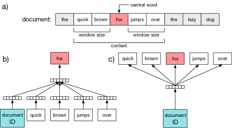
Figure 1. Architecture of the semantic embedding learning tasks, explained using a text document metaphor. a) A sample document, indicating the central word in red and the context words in white, which are defined by the window size. b) The Distributed Memory Model, in which the target word is predicted given the vectors of the document and context words. The lines of small squares represents the learned semantic vectors. c) The Distributed Bag of Words Model, in which the target and context words are predicted given the document’s semantic vector. Figure adapted from Le et al. (Le and Mikolov, 2014).

Other efforts have aimed at encoding temporal aspects of EHR data in the predictive model. Choi and colleagues (Choi et al., 2016a) used time-stamped events as inputs to a particular type of Recurrent Neural Network (RNN) to predict future disease diagnosis. Mehrabi and colleagues (Mehrabi et al., 2015) constructed straightforward temporal matrix representations using codes in rows and years in columns as inputs to a deep Boltzmann machine.

Another interesting recent effort is Rajkomar and colleagues’ (Rajkomar et al., 2018) mapping of raw EHR data to the Fast Healthcare Interoperability Resources (FHIR) format to encode EHR information for several different sequence-oriented models.

All of these approaches rely on preprocessing schemes to prepare the data for use in a model — schemes that are in some cases quite elaborate, require expert tuning or are unique to a specific EHR structure. They can be difficult to compute end-to-end and expensive to train, requiring significant amounts of time and computational resources. In contrast, our approach requires truly minimal preprocessing or tuning, which makes it easily generalizable between institutions.

1.2. Main Contribution

In this paper we propose using a full-record semantic embedding to represent a patient’s entire medical history in a compact but expressive form. The method uses an established embedding algorithm that is relatively easy to implement. It does not rely on extensive data engineering or preprocessing, but takes as input commonly used time-stamped data, making it useful for a wide range of data sources. We show that this representation can be used in several typical medical prediction problems under simple linear models, saving both time and computational resources. This representation is particularly powerful for rapidly testing secondary-use research ideas with EHR data, because it can be precomputed for all patients and then used in downstream modeling by non-experts.

Full source code for the project, including all steps from data extraction through model training, evaluation, and figure generation is publicly available from our Github repository. The datasets themselves cannot be publicly released due to the sensitive nature of medical data.

2. Background

2.1. Medical Taxonomies

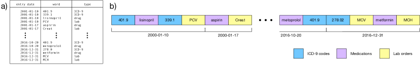
Figure 2. Example input data for one patient record. a) Raw data as obtained from the EHR. b) Data after conversion to a chronological sequence for model training, where events within the same day are ordered randomly.

There are several taxonomies that encode variables of interest in an EHR, including diagnosis and procedure codes, medications names, and laboratory test names, although many of them are not universally adopted. In this section, we briefly describe the taxonomies used in our project.

ICD-9 Codes

Whenever a patient has billable contact with the healthcare system, date-stamped diagnosis codes are attached to the record, indicating the medical conditions that were relevant to the encounter. These codes are notoriously unreliable because, among other things, they are often assigned as a guess before the final diagnosis is known, and they are not revised later (O’Malley et al., 2005). This works fine for billing purposes, but causes obvious trouble if we don’t allow for a high level of noise in these codes. However, when used in aggregate (Denny et al., 2010), and especially if used probabilistically (Lasko, 2014), they can be a valuable source of disease signals.

In our institution, codes from the International Classification of Diseases, Ninth Revision (ICD-9) have historically been used for diagnostic codes, although the Tenth Revision (ICD-10) has recently been adopted. We used only the ICD-9 version in this project.

The ICD-9 hierarchy consists of 21 chapters, each roughly corresponding to a single organ system or pathologic class. Within a chapter, three-digit parent codes indicate a general disease area (such as female breast cancer of any type), and leaf-level codes of up to five digits indicate specialized distinctions within that area. A small number of ICD-9 codes represent medical procedures. The full classification contains over 18,000 unique codes. We used leaf-level codes as part of the input to our embedding models, and parent codes in evaluation cohort definitions.

Phecodes

Because the vocabulary of ICD-9 or other taxonomies is so large, and the distinctions they encode are not always important for research purposes, equivalence classes have been defined to group them into a smaller number of codes. The phecode taxonomy is one such grouper that maps ICD-9 codes down to 1,866 phecodes at leaf level, with each phecode representing a common medical condition (Denny et al., 2010; Wei et al., 2017). We did not use this grouper when training our embedded representation, but we did use it to reduce the dimensionality of the comparison representation for computational tractability (Section 4.1).

ATC codes

The Anatomical Chemical Classification System (ATC) is a multi-level grouper for medications, organized by both anatomic and therapeutic class. As with the phecode grouper, we did not use the ATC grouper to train our embedded representation, but we did use it to reduce the dimensionality of our comparison representation for computational tractability (Section 4.1).

2.2. Semantic embeddings

A semantic embedding is a vector representation of a set of variables that attempts to encode the semantic meaning of each variable in a way that is accessible to downstream computing. Its first demonstration was in learning semantic vectors of words in a document such that words of similar meaning were located near each other in the embedded vector space, and that the relative location of two words in the space could encode a meaningful relationship, such as the relationship of a capital city to a country (Mikolov et al., 2013a).

Two algorithms that were initially proposed were the Continuous Skip-gram Model, in which the learning problem was to predict nearby words (called context words) using the central word’s semantic vector, and the Continuous Bag of Words Model, in which the problem was to predict the central word given the semantic vectors of the context words (Mikolov et al., 2013a).

	Embedding	Breast cancer		Diabetes treatment		Lung cancer
		Positive	Negative	Positive	Negative	Positive	Negative
# of ICD-9 events	79,866,333	300,226	300,248	683,538	683,542	152,331	1,059,198
# of lab events	216,392,248	710,161	741,293	1,476,329	1,554,251	445,196	3,626,106
# of medication events	66,269,824	266,289	271,989	467,408	461,650	147,244	1,118,321
# of total events	362,528,405	1,276,676	1,313,530	2,627,275	2,699,443	744,771	5,803,625
# of unique ICD-9	19,994	7,094	8,261	9,459	10,933	5,600	10,720
# of unique labs	5,509	1,240	1,510	1,643	1,949	1,038	2,117
# of unique codes	31,589	9,671	11,348	12,625	14,756	7,694	14,829
# of patients	2,309,712	2,901	2,901	10,477	10,477	1,104	5,631
months of history	11.8 [0, 67.3]	90.1 [55.6, 132.5]	143.2 [100.9, 186.7]	70 [42.7, 110]	129.1 [87.5, 173.6]	80.1 [49.9, 124.9]	71.6 [43.3, 114.2]
ICD-9 events	8 [3, 27]	51 [25, 122]	51 [25, 122]	39 [21, 76]	39 [21, 76]	79.5 [33, 174]	92 [35, 231]
Lab events	1 [0, 49]	85 [18, 247]	78 [13, 261]	60 [8, 155]	48 [2, 143]	183.5 [48.8, 466.2]	208 [42, 674]
Medication events	2 [0, 14]	23 [4, 87]	26 [7, 88]	11 [2, 43]	16 [4, 46]	49 [10, 157.5]	54 [9, 201.5]
Total events	21 [4, 93]	168 [59, 461]	163 [64, 475]	118 [50, 275]	114 [49, 265]	329.5 [104.8, 792.8]	369 [98, 1130.5]

Table 1. Composition of the data used for embedding and the three evaluation problems. Cells contain either total counts or Median [IQR].

These algorithms were extended to learn a single semantic vector representing an entire document (Le and Mikolov, 2014). One extension, the Distributed Memory Model (Figure 1b), is analogous to the Continuous Bag of Words Model, in which the task is to predict a target word given the vectors of nearby words and the vector of the document as a whole. The second extension is the Distributed Bag of Words Model (Figure 1c), analogous to the Skip-gram Model, in which the task is to predict individual document words given the document vector.

All of these models use a simple neural network architecture in which the dimension of the input and output layers is the size of the vocabulary, and once trained, the hidden layer contains the semantic vectors of interest.

Although these architectures are simple, the number of nodes in them can be very large, which increases training time. To reduce this time, two alternative training methods are commonly used: hierarchical softmax (Morin and Bengio, 2005) and negative sampling (Mnih and Hinton, 2008). Both increase speed by updating only a fraction of all weights per iteration. Hierarchical softmax is a computationally efficient approximation of the softmax function which uses a binary tree representation of all words in the vocabulary. The words themselves are leaves in the tree. For each leaf, there exists a unique path from the root to the leaf, and this path is used to estimate the probability of the word represented by the leaf (Colyer, 2016). Negative sampling is a simplified variant of Noise Contrastive Estimation (NCE) (Gutmann and Hyvärinen, 2012; Mikolov et al., 2013b), where only a sample of output words are updated per iteration. The target output word is kept in the sample and gets updated, but a number of non-targets are added as negative samples (Colyer, 2016).

In this project, we used the document-level embedding approach, treating an entire patient record (which could cover more than 20 years of history) as a document, and the data elements of ICD-9 codes, lab tests, and medications as its words.

3. Patient-Level Embedding Models

We tested both the Distributed Memory Model and the Distributed Bag of Words Model to create record-level embeddings, using both hierarchical softmax and negative sampling approximation methods.

3.1. Data

All data for this project was extracted from the de-identified mirror of Vanderbilt’s Electronic Health Record, which contains administrative data, billing codes, medication exposures, laboratory test results, and narrative text for over 2 million patients, reaching back nearly 30 years (Roden et al., 2008). We obtained IRB approval to use this data in this research.

To train the embedding model, we extracted all ICD-9 billing codes, medication exposures, and laboratory test results from each patient record (Table 1). Data preprocessing was deliberately minimal. ICD-9 code events and generic medication names were used as-is. No attempts at synonym detection, grouping, or typographical error correction were made. Laboratory test results were represented only as measurement events, labeled by test name and time, ignoring the numeric result. For historical reasons, many nearly identical laboratory tests were represented by distinct identifiers, and we did not attempt to group them. The only transformation step was to remove vocabulary elements appearing less than 250 times in the dataset (out of 363 million total events), resulting in a final vocabulary size of 31,589.

For each record, these elements were ordered by the sequence of their appearance (Figure 2). Order within the same day was randomized because some events included only date information.

A total of 2,309,712 patient records and 362,528,405 events were used to train the model.

3.2. Model Training

We computed an embedded representation for each patient record using both the Distributed Bag of Words Model and Distributed Memory Model architectures. For each architecture, all combinations of embedding dimension (10, 50, 100, 300, 500, 1000), sliding window sizes (5, 10, 20, 30, 50), and softmax approximation methods (hierarchical softmax, negative sampling) were trained and evaluated.

Embedding models were trained for 20 iterations, with convergence usually after 5 - 10 iterations. After initial evaluation (Table 2), the top 15 performing models were trained for an additional 60 iterations.

All models were generated using Gensim (Řehůřek and Sojka, 2010), an open-source Python library for statistical semantic analysis and natural language processing.

4. Evaluation

algorithm		Distributed Memory version of Paragraph Vector										Distributed Bag of Words version of Paragraph Vector
softmax		Hierarchical Softmax					Negative Sampling					Hierarchical Softmax					Negative Sampling
window size		5	10	20	30	50	5	10	20	30	50	5	10	20	30	50	5	10	20	30	50
embedding size	10	0.71	0.70	0.64	0.60	0.61	0.72	0.68	0.66	0.63	0.60	0.79	0.78	0.79	0.79	0.78	0.79	0.78	0.81	0.79	0.81
	50	0.79	0.75	0.71	0.70	0.66	0.75	0.73	0.69	0.66	0.67	0.83	0.82	0.81	0.83	0.83	0.80	0.81	0.81	0.81	0.81
	100	0.80	0.77	0.73	0.72	0.67	0.77	0.74	0.70	0.71	0.66	0.83	0.82	0.82	0.83	0.83	0.82	0.83	0.79	0.82	0.81
	300	0.80	0.77	0.73	0.72	0.71	0.77	0.72	0.72	0.69	0.69	0.82	0.84	0.84	0.82	0.82	0.82	0.82	0.82	0.82	0.81
	500	0.79	0.78	0.73	0.72	0.70	0.78	0.74	0.73	0.71	0.70	0.82	0.81	0.82	0.81	0.82	0.80	0.82	0.80	0.80	0.79
	1000	0.79	0.77	0.73	0.74	0.71	0.76	0.75	0.69	0.72	0.72	0.81	0.83	0.82	0.82	0.81	0.79	0.79	0.80	0.80	0.81

Table 2. Effects of varying the embedding parameters. The Distributed Bag of Words approach is a clear winner in our problems, with performance being fairly invariant to other parameters away from the extremes. The number in each cell is the AUC of the gradient tree boosting model with default parameters predicting breast cancer diagnosis with a 12-month prediction horizon (boosting model parameters were optimized subsequent to this step). Dark purple color represents the worst performance, bright yellow the best.

To evaluate the extent to which the embedded representations preserve, decrease, or augment the predictive value of the original data, we compared the performance of those representations to that of a simple but common representation of the same information on three different clinical tasks, each task being representative of a typical and meaningful predictive problem in the clinical domain. For each problem we trained a simple linear model and a complex nonlinear model, comparing the performance of our embedded representation with that of a simple but traditional summary representation. The goal of the evaluation was not to achieve state-of-the-art performance on each problem, but to gain insight into the tradeoffs of the embedded representation vs. the simple one. There are certainly more complex models (such as sequence-based models (Bajor and A., 2017; Luo, 2017; Pham et al., 2017; Choi et al., 2017) or deep feed-forward networks (Ching et al., 2018; Miotto et al., 2017, 2016a; Lasko et al., 2013)) that could probably squeeze a little more performance out of the data for each problem, but they would require much greater computational effort, and using them here would not appreciably alter our conclusions.

We used the linear model to understand the degree to which the semantic embedding captures complex, nonlinear dependencies in the data, and the nonlinear model to understand the degree to which the embedding loses predictive information. We expect the embedded representation to outperform the simple representation on the linear model if it managed to capture meaningful dependencies between elements. We expect it to under-perform the simple representation on the nonlinear model if the embedding irretrievably loses predictive information. Finally, we can compare the ability of the embedding to capture complex dependencies to the ability of the model to capture those dependencies by comparing the performance of the embedded representation under the simple model to the simple representation under the complex model.

In addition to this objective evaluation, we also subjectively investigated the extent to which the embedding captures information about patient state and disease trajectory by generating a visualization of patients in the embedded space and the changes that occur as a disease process progresses.

4.1. Data

Data for the evaluations was drawn from the same source as the embedding models, although it required some additional preprocessing to identify the proper cohorts and assign labels. For each test problem, input data was collected from the repository for each patient record up until a given problem-specific cutoff date (see below). The embedded representation and simple representation were then computed from that time-truncated data.

Simple Representation

The simple representation we used was a counted bag-of-words vector, where a word in this case is the appearance of a lab test, medication exposure, or ICD-9 code in the record. This is a very common representation for medical prediction projects (Liao et al., 2010; Carroll et al., 2012; Sun et al., 2014; Pivovarov et al., 2015). However, the large vocabulary this produced (31,520 elements) was computationally intractable for our models, so we reduced it by grouping ICD-9 codes into phecodes, and by grouping medications to their ATC therapeutic class equivalence (Section 2.1). The final number of features after grouping was between 3639 and 4535, after removing features with 0 total counts in each problem. The sparsity of this representation was very high, even after grouping.

Embedded Representation

Once the semantic embedding models were trained, we projected the time-truncated test data into the embedded space in the usual way, which is to run the training algorithm one more iteration with the single addition of the new instance.

4.2. Objective Evaluation

We objectively evaluated the embedding models by assessing how well they perform as input representations for three clinical prediction problems, comparing them to the performance of the same information in the simple representation.

Each prediction problem was expanded into five tasks with increasingly difficult prediction horizons, or the time between the input data cutoff date and the event to be predicted. We used prediction horizons of 1 day and 1, 3, 6, and 12 months. For each task we evaluated discrimination using the area under the Receiver Operating Characteristic Curve (AUC), and calibration using observed to expected probabilities in bins over the range of prediction.

The linear model was a simple elastic net (Scikit-learn implementation) (Pedregosa et al., 2011), with parameters optimized by cross-validation.

The nonlinear model was the XGBoost implementation of gradient tree boosting, also known as a gradient boosting machine (GBM) (Chen and Guestrin, 2016). This model is extremely effective at extracting meaningful dependencies in the input data, and often achieves state-of-the art results. In 2015, 17 out of 29 winning solutions in Kaggle competitions used XGBoost (Chen and Guestrin, 2016). Its drawback is that training and parameter optimization requires considerable computational time.

In our experiments, a grid search over embedding parameters using default XGBoost parameters was the first pass at optimization (Table 2), and then the top 15 embedding parameter settings were chosen and XGBoost parameters optimized with random search for each of those embeddings.

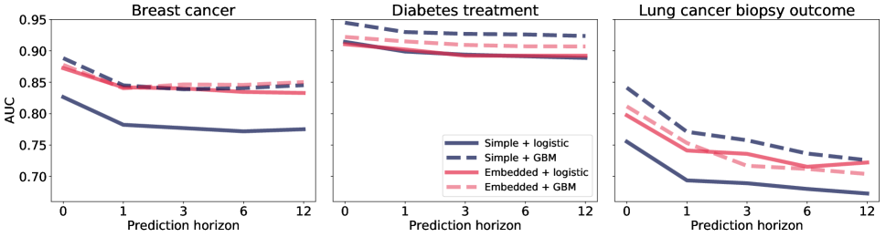
Figure 3. Capture and loss of complex data dependencies. Where the red solid line is above the blue solid line, it indicates the capture of complex dependencies by the embedded representation. Where the blue dashed line is above the red dashed line, it indicates loss of complex information by the embedded representation. Where the blue dashed line is above the red solid line, it indicates information captured by the complex model that was missed by the embedded representation.

Female Breast Cancer Prediction Problem

The first evaluation problem was to predict whether a female patient would develop breast cancer at the prediction horizon. Female subjects with at least 10 recorded ICD-9 codes of any type and at least 24 months of data before the cutoff date were considered for the dataset. Records with at least 3 codes with an ICD-9 174-parent (Malignant neoplasm of female breast) were labeled positive, and their cutoff date was the first of those 174-parent events. Records with no 174-parent codes at all were labeled negative. Their cutoff date was set arbitrarily to the day when raw data was pulled from the database for the experiment.

The raw number of negative instances was much higher than number of positive instances, but negative instances were then selected to match positive instances as closely as possible on the number of total ICD-9 codes and the time length of the record (Table 1). After matching, we had the same number of negative and positive instances. A stratified split was then performed to divide the dataset into training (75%), test (20%) and validation (5%) sets.

Diabetes Treatment Prediction Problem

The second evaluation problem was to predict whether a given patient would begin treatment for type 2 diabetes at the prediction horizon. We used the start of medical treatment rather than the date of diagnosis because it is a cleaner event that is easier to identify from the data in the record. For type 2 diabetes, medical treatment generally begins with an oral glucose-lowering drug, and we used the start of such a drug to define the prediction target.

All records selected for this task had at least 10 ICD-9 codes of any type and at least 24 months of data before the cutoff date. Records with at least 10 mentions of a medication in the ATC category A10B: Blood glucose lowering drugs, excluding insulins, and which did not have a prior record of taking insulin, were labeled as positive instances. The cutoff date was set as the first mention of such a drug. Records with no mention of any drug in the broader ATC category A10: Drugs used in diabetes were labeled as negative instances, with a cutoff date arbitrarily set as the day when raw data was pulled for the experiment.

As above, negative instances were matched to positive instances on the total number of ICD-9 codes and the time length of the medical record (Table 1). A stratified split was performed to divide the dataset into training (75%), test (20%) and validation (5%) sets.

Lung Cancer Prediction Problem

The final evaluation problem was to predict whether a patient undergoing a lung biopsy would be diagnosed with lung cancer within the prediction horizon. This prediction covers the case where the biopsy was immediately positive and treatment begun, as well as the case where the biopsy might be immediately negative, but lung cancer developed at some later point within the prediction horizon.

Records with at least 10 ICD-9 codes of any type and at least 24 months of data before the cutoff date were considered for the dataset. They all had either an ICD-9 code from the 33.2 group (Diagnostic Procedures On Lung And Bronchus) or a procedure code for a lung biopsy. All instances used the code for the first lung biopsy as the cutoff date. Instances with at least two downstream codes with an ICD-9 162 parent (Malignant neoplasm of trachea bronchus and lung) were labeled as positive, and instances with no codes from that parent were labeled negative.

Because both positive and negative instances were selected by the presence of a lung biopsy, matching was not needed to reduce information leaking from the selection criteria. The positive cohort contained of 1104 instances, while the negative cohort contained 5631 instances. A stratified split was performed to divide the dataset into training (75%), test (20%) and validation (5%) sets.

4.3. Subjective Evaluation

We subjectively explored the properties of the embedding by visualizing the embedded patient space in two dimensions. To understand the degree to which similar patients were placed nearby in the space, we projected the positive instances, negative instances, and some randomly sampled additional records into the first two principal components of the embedding space and plotted this for each of the prediction problems. The principal components were computed separately for the input dataset of each problem.

And finally, to understand the degree to which the embedding captures the notion of a disease trajectory in this space, we looked at several longitudinal trajectories of individual records, overlaying them onto the 2-dimensional projection.

5. Results and Discussion

Objectively, the embedded models were robust to most architecture choices and parameter settings, and they captured a large fraction of the complex dependencies in the data, although in some cases the compression did lose information. Subjectively, the embeddings capture quite well the notions of patient similarity and disease trajectory.

5.1. Embedding Model Architecture

For these problems the Distributed Bag of Words Model outperformed the Distributed Memory Model by a fair amount, but otherwise performance was robust to changes in embedding model parameters; there was a slight preference for hierarchical softmax over negative sampling, and no substantial effect of embedding dimension above about 50 (Table 2). For the Distributed Bag of Words Model, there was no systematic preference for large vs. small window sizes, although for the Distributed Memory Model smaller windows worked better.

5.2. Prediction Tasks

The prediction task results demonstrate that the embedding manages to capture a large fraction of the data dependencies with minimal loss, although the degree of each of these varied by task (Figure 3).

In the breast cancer prediction, the embedded representation captured as much complex information as the complex model did, with no apparent information loss. This is the best we could hope for with the performance of the embedding; if it were always true, it would mean we could routinely store the complex dependencies in the data representation, and then use fast, simple linear models for all of our prediction tasks.

However, in the diabetic treatment prediction, the embedded representation provided no improvement over the simple representation, indicating its failure to extract additional information from the data. On the other hand, the small improvements under the complex model suggest that there was little increase to be had. In this case, there was only a small amount of additional structure available in the data to improve the prediction (which was already very accurate without using any complex interaction information), and this small additional structure was picked up only by the complex model. And in fact, some of that small additional dependence information was lost by the embedding.

Finally, in the lung cancer prediction, the embedded representation captured much additional structure, more than half of what was captured by the complex model, although there was also some information lost.

The calibration of predictions was not changed much by the choice of representation (Figure 4). Of the small differences, calibration of the linear model was always slightly better for the embedded representation, and for the complex model it was slightly better for the simple representation. The calibration for both representations was poor for the linear model of lung cancer.

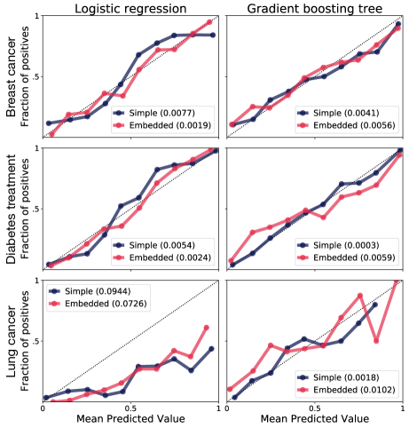
Figure 4. Calibration was largely unaffected by the choice of representation for any problem. Dotted line is the expected value for a perfect calibration. Value in parentheses is the MSE over all bins of observed vs. expected. Data shown is for a 1 day prediction horizon, and is typical of other cases.

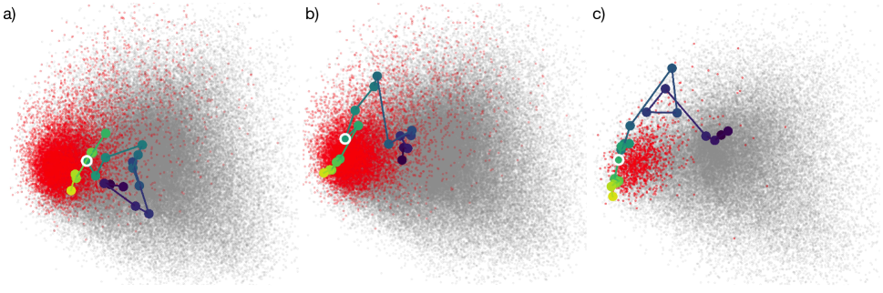
Figure 5. The embedded representation preserves notions of patient similarity and disease trajectory for all three problems: a) Breast cancer prediction, b) Diabetes treatment prediction, c) Lung cancer prediction. Each small dot represents a patient record projected onto the first 2 principal components for each dataset. Red dots are positive labeled records, which cluster tightly in each case, indicating the preservation of patient similarity. Grey dots are negative records plus a large sample of random records from the embedding dataset. A single patient trajectory is overlaid in each figure, where the passage of time is indicated by a progression of dark purple to yellow color. A white circle indicates the time when the diagnosis was made or the treatment started. In all cases the patient starts out negative and outside the cluster, and progresses to positive inside the cluster.

5.3. Subjective Analysis

The embedded vectors subjectively do a great job of encoding patient state in a way that enables simple similarity metrics and disease trajectory visualizations (Figure 5). We evaluated a couple dozen of these visualizations, and we show here a representative case from each problem. Each panel shows the same embedding space, but projected onto the first two principal components for the corresponding problem. In each panel the positive instances are clustered tightly in one area of the projection, although there is some fade between the positive and negative instances. The fade may be due to undiagnosed illness, label noise, limitations in the projection, or limitations in the embedding. The patient trajectories each illustrate the disease progression of a single patient from having no disease and located among the negative instances, to having the disease and located among the positive instances. The diagnosis of the disease or the start of treatment happens as they cross the boundary to the positive cases. Static and animated GIF images of trajectories for more patients are available in our code repository.

5.4. Conclusions

This work demonstrates merit in the idea of capturing complex data dependencies and storing them in the data representation instead of in the prediction model, especially if the original data is as messy as clinical data. The advantages of using a record-level semantic embedding for such a representation are that the complexity can be captured independent of any particular learning problem, stored much more compactly than the original data, and then used with simple, fast linear models for prediction.

This type of design may work especially well for initial, proof-of-concept experiments, such as rough-cut cohort definitions where the trade-off between accuracy and time-to-result falls preferentially toward getting faster answers. The generic nature of the representation and the fact that it is computed in an unsupervised way also lends itself to situations where hundreds or thousands of approximate models need to be built, such as to predict whether the patient will develop any of the 18,000 conditions described by ICD-9 codes. There may be more powerful and accurate ways to train models to do that, but the cost in computing time and software engineering effort may not be worth it for some use cases.

One way to improve our results may be to add more data types that are found in a typical EHR. Clinical notes could be added in the usual way for training semantic embeddings, and other structured data such as vital signs measurements could also be added. This is the focus of future work.

The method presented here provides a promising rapid research approach for researchers working with EHR data, as well as knowledge discovery and exploration of complicated, heterogeneous datasets more broadly.

References

- (1)
- Bajor and A. (2017) Jacek M. Bajor and Lasko Thomas A. 2017. Predicting medications from diagnostic codes with recurrent neural networks. In 5th International Conference on Learning Representations. https://openreview.net/pdf?id=rJEgeXFex.
- Beaulieu-Jones and Greene (2016) Brett K. Beaulieu-Jones and Casey S. Greene. 2016. Semi-supervised learning of the electronic health record for phenotype stratification. Journal of Biomedical Informatics 64, Supplement C (2016), 168 – 178. https://doi.org/10.1016/j.jbi.2016.10.007
- Bowton et al. (2014) E. Bowton, J. R. Field, S. Wang, J. S. Schildcrout, S. L. Van Driest, J. T. Delaney, J. Cowan, P. Weeke, J. D. Mosley, Q. S. Wells, J. H. Karnes, C. Shaffer, J. F. Peterson, J. C. Denny, D. M. Roden, and J. M. Pulley. 2014. Biobanks and electronic medical records: enabling cost-effective research. Science Translational Medicine 6, 234 (Apr 2014), 234cm3.
- Carroll et al. (2012) Robert J Carroll, Will K Thompson, Anne E Eyler, Arthur Mandelin, Tianxi Cai, Raquel M Zink, Jennifer A Pacheco, Chad Boomershine, Thomas A Lasko, Hua Xu, Elizabeth W Karlson, Raul G Perez, Vivian Gainer, Shawn N Murphy, Eric Ruderman, Richard Pope, Robert M Plenge, Abel Ngo Kho, Katherine P Liao, and Joshua Denny. 2012. Portability of an algorithm to identify rheumatoid arthritis in electronic health records. Journal of the American Medical Informatics Association 19 (02 2012), e162–e169.
- Chen and Guestrin (2016) Tianqi Chen and Carlos Guestrin. 2016. XGBoost: A scalable tree boosting system. CoRR abs/1603.02754 (2016). arXiv:1603.02754 http://arxiv.org/abs/1603.02754
- Ching et al. (2018) Travers Ching, Daniel S Himmelstein, Brett K Beaulieu-Jones, Alexandr A Kalinin, Brian T Do, Gregory P Way, Enrico Ferrero, Paul-Michael Agapow, Michael Zietz, Michael M Hoffman, et al. 2018. Opportunities and obstacles for deep learning in biology and medicine. bioRxiv (2018), 142760.
- Choi et al. (2016a) Edward Choi, Mohammad Taha Bahadori, Andy Schuetz, Walter F Stewart, and Jimeng Sun. 2016a. Doctor AI: Predicting clinical events via recurrent neural networks. In Machine Learning for Healthcare Conference. 301–318.
- Choi et al. (2016b) Edward Choi, Mohammad Taha Bahadori, Elizabeth Searles, Catherine Coffey, and Jimeng Sun. 2016b. Multi-layer representation learning for medical concepts. CoRR abs/1602.05568 (2016). arXiv:1602.05568 http://arxiv.org/abs/1602.05568
- Choi et al. (2016c) Edward Choi, Andy Schuetz, Walter F. Stewart, and Jimeng Sun. 2016c. Medical concept representation learning from electronic health records and its application on heart failure prediction. CoRR abs/1602.03686 (2016). arXiv:1602.03686 http://arxiv.org/abs/1602.03686
- Choi et al. (2017) Edward Choi, Andy Schuetz, Walter F Stewart, and Jimeng Sun. 2017. Using recurrent neural network models for early detection of heart failure onset. Journal of the American Medical Informatics Association 24, 2 (2017), 361–370. https://doi.org/10.1093/jamia/ocw112
- Colyer (2016) Adrian Colyer. 2016. The amazing power of word vectors. (2016). https://blog.acolyer.org/2016/04/21/the-amazing-power-of-word-vectors/
- Denny et al. (2010) Joshua C. Denny, Marylyn D. Ritchie, Melissa A. Basford, Jill M. Pulley, Lisa Bastarache, Kristin Brown-Gentry, Deede Wang, Dan R. Masys, Dan M. Roden, and Dana C. Crawford. 2010. PheWAS: demonstrating the feasibility of a phenome-wide scan to discover gene–disease associations. Bioinformatics 26, 9 (2010), 1205–1210. https://doi.org/10.1093/bioinformatics/btq126 arXiv:http://bioinformatics.oxfordjournals.org/content/26/9/1205.full.pdf+html
- Gutmann and Hyvärinen (2012) M.U. Gutmann and A. Hyvärinen. 2012. Noise-contrastive estimation of unnormalized statistical models, with applications to natural image statistics. Journal of Machine Learning Research 13 (2 2012), 307–361.
- Kohane (2011) Isaac S. Kohane. 2011. Using electronic health records to drive discovery in disease genomics. Nature Reviews Genetics 12, 6 (June 2011), 417 – 428.
- Lasko (2014) Thomas A. Lasko. 2014. Efficient inference of Gaussian process modulated renewal processes with application to medical event data. Uncertainty in Artificial Intelligence - Proceedings of the 30th Conference 2014 (02 2014).
- Lasko et al. (2013) Thomas A Lasko, Joshua C Denny, and Mia A Levy. 2013. Computational phenotype discovery using unsupervised feature learning over noisy, sparse, and irregular clinical data. PLOS ONE 8, 6 (2013), e66341.
- Le and Mikolov (2014) Quoc V. Le and Tomas Mikolov. 2014. Distributed representations of sentences and documents. CoRR abs/1405.4053 (2014). arXiv:1405.4053 http://arxiv.org/abs/1405.4053
- Liao et al. (2010) Katherine P Liao, Tianxi Cai, Vivian Gainer, Sergey Goryachev, Qing Zeng-Treitler, Soumya Raychaudhuri, Peter Szolovits, Susanne Churchill, Shawn Murphy, Isaac Kohane, Elizabeth W Karlson, and Robert M Plenge. 2010. Electronic medical records for discovery research in rheumatoid arthritis. Arthritis care & research 62 (08 2010), 1120–7.
- Luo (2017) Yuan Luo. 2017. Recurrent neural networks for classifying relations in clinical notes. Journal of Biomedical Informatics 72 (2017), 85–95.
- Mehrabi et al. (2015) Saaed Mehrabi, Sunghwan Sohn, Dingheng Li, Joshua J Pankratz, Terry Therneau, Jennifer L St Sauver, Hongfang Liu, and Mathew Palakal. 2015. Temporal pattern and association discovery of diagnosis codes using deep learning. In Healthcare Informatics (ICHI), 2015 International Conference on. IEEE, 408–416.
- Mikolov et al. (2013a) Tomas Mikolov, Kai Chen, Greg Corrado, and Jeffrey Dean. 2013a. Efficient estimation of word representations in vector space. CoRR abs/1301.3781 (2013). arXiv:1301.3781 http://arxiv.org/abs/1301.3781
- Mikolov et al. (2013b) Tomas Mikolov, Ilya Sutskever, Kai Chen, Greg Corrado, and Jeffrey Dean. 2013b. Distributed representations of words and phrases and their compositionality. CoRR abs/1310.4546 (2013). arXiv:1310.4546 http://arxiv.org/abs/1310.4546
- Miotto et al. (2016a) Riccardo Miotto, Li Li, and Joel T Dudley. 2016a. Deep learning to predict patient future diseases from the electronic health records. In European Conference on Information Retrieval. Springer, 768–774.
- Miotto et al. (2016b) Riccardo Miotto, Li Li, Brian A. Kidd, and Joel T. Dudley. 2016b. Deep Patient: An unsupervised representation to predict the future of patients from the electronic health records. Scientific Reports 6 (17 05 2016), 26094 EP –. http://dx.doi.org/10.1038/srep26094
- Miotto et al. (2017) Riccardo Miotto, Fei Wang, Shuang Wang, Xiaoqian Jiang, and Joel T Dudley. 2017. Deep learning for healthcare: review, opportunities and challenges. Briefings in bioinformatics (2017).
- Mnih and Hinton (2008) Andriy Mnih and Geoffrey Hinton. 2008. A scalable hierarchical distributed language model. In Neural Information Processing Systems.
- Morin and Bengio (2005) Frederic Morin and Yoshua Bengio. 2005. Hierarchical probabilistic neural network language model. In AISTATS.
- Nguyen et al. (2017) Phuoc Nguyen, Truyen Tran, Nilmini Wickramasinghe, and Svetha Venkatesh. 2017. Deepr: A convolutional net for medical records. IEEE Journal of Biomedical and Health Informatics 21, 1 (2017), 22–30.
- O’Malley et al. (2005) K. J. O’Malley, K. F. Cook, M. D. Price, K. R. Wildes, J. F. Hurdle, and C. M. Ashton. 2005. Measuring diagnoses: ICD code accuracy. Health Services Research 40, 5 Pt 2 (Oct 2005), 1620–1639.
- Pedregosa et al. (2011) F. Pedregosa, G. Varoquaux, A. Gramfort, V. Michel, B. Thirion, O. Grisel, M. Blondel, P. Prettenhofer, R. Weiss, V. Dubourg, J. Vanderplas, A. Passos, D. Cournapeau, M. Brucher, M. Perrot, and E. Duchesnay. 2011. Scikit-learn: Machine learning in Python. Journal of Machine Learning Research 12 (2011), 2825–2830.
- Pham et al. (2016) Trang Pham, Truyen Tran, Dinh Phung, and Svetha Venkatesh. 2016. DeepCare: A deep dynamic memory model for predictive medicine. In Pacific-Asia Conference on Knowledge Discovery and Data Mining. Springer, 30–41.
- Pham et al. (2017) Trang Pham, Truyen Tran, Dinh Phung, and Svetha Venkatesh. 2017. Predicting healthcare trajectories from medical records: A deep learning approach. Journal of Biomedical Informatics 69 (2017), 218–229.
- Pivovarov et al. (2015) Rimma Pivovarov, Adler J. Perotte, Edouard Grave, John Angiolillo, Chris H. Wiggins, and Noémie Elhadad. 2015. Learning probabilistic phenotypes from heterogeneous EHR data. Journal of Biomedical Informatics 58, Supplement C (2015), 156 – 165. https://doi.org/10.1016/j.jbi.2015.10.001
- Rajkomar et al. (2018) A. Rajkomar, E. Oren, K. Chen, A. M. Dai, N. Hajaj, P. J. Liu, X. Liu, M. Sun, P. Sundberg, H. Yee, K. Zhang, G. E. Duggan, G. Flores, M. Hardt, J. Irvine, Q. Le, K. Litsch, J. Marcus, A. Mossin, J. Tansuwan, D. Wang, J. Wexler, J. Wilson, D. Ludwig, S. L. Volchenboum, K. Chou, M. Pearson, S. Madabushi, N. H. Shah, A. J. Butte, M. Howell, C. Cui, G. Corrado, and J. Dean. 2018. Scalable and accurate deep learning for electronic health records. ArXiv e-prints (Jan. 2018). arXiv:cs.CY/1801.07860
- Řehůřek and Sojka (2010) Radim Řehůřek and Petr Sojka. 2010. Software framework for topic modelling with large corpora. In Proceedings of the LREC 2010 Workshop on New Challenges for NLP Frameworks. ELRA, Valletta, Malta, 45–50. http://is.muni.cz/publication/884893/en.
- Roden et al. (2008) D. M. Roden, J. M. Pulley, M. A. Basford, G. R. Bernard, E. W. Clayton, J. R. Balser, and D. R. Masys. 2008. Development of a large-scale de-identified DNA biobank to enable personalized medicine. Clinical Pharmacology & Therapeutics 84, 3 (Sep 2008), 362–369.
- Safran et al. (2007) Charles Safran, Meryl Bloomrosen, W Edward Hammond, Steven Labkoff, Suzanne Markel-Fox, Paul C. Tang, Don E. Detmer, and Expert Panel. 2007. Toward a national framework for the secondary use of health data: an American Medical Informatics Association White Paper. Journal of the American Medical Informatics Association 14, 1 (2007), 1–9. https://doi.org/10.1197/jamia.M2273
- Shickel et al. (2017) Benjamin Shickel, Patrick James Tighe, Azra Bihorac, and Parisa Rashidi. 2017. Deep EHR: A survey of recent advances in deep learning techniques for electronic health record (EHR) analysis. IEEE Journal of Biomedical and Health Informatics (2017).
- Sun et al. (2014) Jimeng Sun, Candace D McNaughton, Ping Zhang, Adam Perer, Aris Gkoulalas-Divanis, Joshua C Denny, Jacqueline Kirby, Thomas Lasko, Alexander Saip, and Bradley A Malin. 2014. Predicting changes in hypertension control using electronic health records from a chronic disease management program. Journal of the American Medical Informatics Association 21, 2 (2014), 337–344. https://doi.org/10.1136/amiajnl-2013-002033 arXiv:https://academic.oup.com/jamia/article-pdf/21/2/337/6114230/21-2-337.pdf
- Wei et al. (2017) Wei-Qi Wei, Lisa A. Bastarache, Robert J. Carroll, Joy E. Marlo, Travis J. Osterman, Eric R. Gamazon, Nancy J. Cox, Dan M. Roden, and Joshua C. Denny. 2017. Evaluating phecodes, clinical classification software, and ICD-9-CM codes for phenome-wide association studies in the electronic health record. PLOS ONE 12, 7 (07 2017), 1–16. https://doi.org/10.1371/journal.pone.0175508
- Weiskopf and Weng (2013) N. G. Weiskopf and C. Weng. 2013. Methods and dimensions of electronic health record data quality assessment: enabling reuse for clinical research. Journal of the American Medical Informatics Association 20, 1 (Jan 2013), 144–151.
- Wilke et al. (2011) R. A. Wilke, H. Xu, J. C. Denny, D. M. Roden, R. M. Krauss, C. A. McCarty, R. L. Davis, T. Skaar, J. Lamba, and G. Savova. 2011. The emerging role of electronic medical records in pharmacogenomics. Clinical Pharmacology & Therapeutics 89, 3 (Mar 2011), 379–386.