KINEMATIC DISTANCES: A MONTE CARLO METHOD

Abstract

Distances to high mass star forming regions (HMSFRs) in the Milky Way are a crucial constraint on the structure of the Galaxy. Only kinematic distances are available for a majority of the HMSFRs in the Milky Way. Here we compare the kinematic and parallax distances of 75 Galactic HMSFRs to assess the accuracy of kinematic distances. We derive the kinematic distances using three different methods: the traditional method using the Brand & Blitz (1993) rotation curve (Method A), the traditional method using the Reid et al. (2014) rotation curve and updated Solar motion parameters (Method B), and a Monte Carlo technique (Method C). Methods B and C produce kinematic distances closest to the parallax distances, with median differences of $13\%$ ($0.43\,{\rm kpc}$) and $17\%$ ($0.42\,{\rm kpc}$), respectively. Except in the vicinity of the tangent point, the kinematic distance uncertainties derived by Method C are smaller than those of Methods A and B. In a large region of the Galaxy, the Method C kinematic distances constrain both the distances and the Galactocentric positions of HMSFRs more accurately than parallax distances. Beyond the tangent point along $\ell=30^{\circ}$, for example, the Method C kinematic distance uncertainties reach a minimum of $10\%$ of the parallax distance uncertainty at a distance of $14\,{\rm kpc}$. We develop a prescription for deriving and applying the Method C kinematic distances and distance uncertainties. The code to generate the Method C kinematic distances is publicly available and may be utilized through an on-line tool.

1 Introduction

Revealing the morphological and chemical structure of the Milky Way requires knowing the locations of objects on a Galaxy-wide scale. In the Solar neighborhood, the distances to stars can be accurately derived by measuring their parallax. Far from the Solar neighborhood, distances to stars may be determined using spectrophotometric techniques (e.g., Moisés et al., 2011) and red clump stars (e.g., Bovy et al., 2014). Distances to gas clouds can be gotten from both Very Long Baseline Interferometry (VLBI) parallax measurements of molecular maser emission from high mass star forming regions (HMSFRs) (e.g., Reid et al., 2014) as well as kinematic distance determinations (e.g., Anderson et al., 2012).

Kinematic distances are derived by measuring the local standard of rest (LSR) velocity, $V_{\rm LSR}$, of an object and assuming a model of Galactic rotation. If the object is on a circular orbit following this Galactic rotation model (GRM), then the LSR velocity of the object uniquely identifies the object’s Galactocentric radius, $R$. Beyond the Solar orbit, this technique also uniquely determines the object’s Galactocentric azimuth, $\theta$, and distance from the Sun, $d$. Within the Solar orbit, kinematic distances suffer from the kinematic distance ambiguity (KDA). Here, a single LSR velocity may correspond to two distances: a “near” and “far” kinematic distance. We must use additional information to identify the kinematic distance ambiguity resolution (KDAR). The kinematic method is commonly used to determine the distances to HMSFRs in the study of Galactic structure. Recently, for example, Balser et al. (2015) used H ii region kinematic distances to probe the metallicity distribution across the Galactic disk.

The Green Bank Telescope H ii Region Discovery Survey (GBT HRDS) and its successors discovered more than ${\sim}1000$ new Galactic H ii regions by measuring their centimeter wavelength radio recombination line (RRL) emission (Bania et al., 2010, 2012; Anderson et al., 2015). H ii regions are the zones of ionized gas surrounding recently-formed high-mass (OB-type) stars. They are the archetypical tracer of Galactic spiral structure. Anderson et al. (2012) derived the kinematic distances to 149 H ii regions in the original GBT HRDS, and today the WISE Catalog of Galactic H ii Regions (Anderson et al., 2014) lists ${\sim}1500$ H ii region kinematic distances.

Errors in kinematic distances are caused by both inaccurate GRMs and incorrect KDARs. The rotation of the Milky Way is affected by non-circular streaming motions induced by the Galactic bar and spiral arms (e.g., Burton, 1971; Gómez, 2006; Moisés et al., 2011). These deviations from circular motion will affect the accuracy of GRMs. A variety of techniques have been used to resolve the KDA for Galactic H ii regions, for example, H i emission/absorption experiments (Kuchar & Bania, 1994; Kolpak et al., 2003; Anderson & Bania, 2009; Anderson et al., 2012; Urquhart et al., 2012; Brown et al., 2014), H i self-absorption experiments (Roman-Duval et al., 2009; Urquhart et al., 2012), and H₂CO absorption experiments (Araya et al., 2002; Watson et al., 2003; Sewilo et al., 2004). If these KDAR techniques are inaccurate, the derived kinematic distances will be as well.

Very Long Baseline Interferometric (VLBI) trigonometric parallax measurements of molecular masers are an independent and accurate way to measure the distances to HMSFRs. Over the past decade, the Bar and Spiral Structure Legacy Survey (BeSSeL), the Japanese VLBI Exploration of Radio Astrometry (VERA), and the European VLBI Network (EVN) projects have accumulated a sample of more than 100 VLBI parallaxes and proper motions for masers associated with HMSFRs (Reid et al., 2014). These trigonometrically-derived distances do not suffer from the same problems as kinematic distances. With a typical parallax uncertainty of ${\sim}20\,\mu\text{as}$, these parallax distances are accurate to about 10% at distances of 5$\,{\rm kpc}$ (Reid & Honma, 2014).

Although parallaxes are the “gold standard” distances for HMSFRs, they are difficult and time-consuming to measure. To constrain the parallax and proper motion of four HMSFRs, including W51 Main/South, Sato et al. (2010) used the National Radio Astronomy Observatory (NRAO) Jansky Very Large array to locate background extragalactic position reference objects together with the NRAO Very Long Baseline Array (VLBA) for the accurate astrometry. The VLBA observations totaled ${\sim}28$ hours spread over ${\sim}12$ months. Such observations are impractical to make for all ${\sim}4000$ H ii regions in the WISE Catalog. Furthermore, the majority of the H ii regions in the WISE Catalog will not have detectable maser emission.

Table 1: HMSFR Sample

Name	Alias	RA (J2000)	Decl. (J2000)	Parallax				$V_{\rm LSR}$	Refs.
		(hh:mm:ss)	(dd:mm:ss)	(mas)				(km s-1)
G015.03$-$00.67	M 17	18:20:24.81	$-$16:11:35.3	0.505	0.033 $\pm\!$	22	3	10
G016.58$-$00.05		18:21:09.08	$-$14:31:48.8	0.279	0.023 $\pm\!$	60	5	4
G023.00$-$00.41		18:34:40.20	$-$09:00:37.0	0.218	0.017 $\pm\!$	80	3	11
G023.44$-$00.18		18:34:39.19	$-$08:31:25.4	0.170	0.032 $\pm\!$	97	3	11
G023.65$-$00.12		18:34:51.59	$-$08:18:21.4	0.313	0.039 $\pm\!$	83	3	12
G023.70$-$00.19		18:35:12.36	$-$08:17:39.5	0.161	0.024 $\pm\!$	73	5	7
G025.70+00.04		18:38:03.14	$-$06:24:15.5	0.098	0.029 $\pm\!$	93	5	4
G027.36$-$00.16		18:41:51.06	$-$05:01:43.4	0.125	0.042 $\pm\!$	92	3	10
G028.86+00.06		18:43:46.22	$-$03:35:29.6	0.135	0.018 $\pm\!$	100	10	4
G029.86$-$00.04		18:45:59.57	$-$02:45:06.7	0.161	0.020 $\pm\!$	100	3	6
G029.95$-$00.01	W 43S	18:46:03.74	$-$02:39:22.3	0.190	0.019 $\pm\!$	98	3	6
G031.28+00.06		18:48:12.39	$-$01:26:30.7	0.234	0.039 $\pm\!$	109	3	6
G031.58+00.07	W 43Main	18:48:41.68	$-$01:09:59.0	0.204	0.030 $\pm\!$	96	5	6
G032.04+00.05		18:49:36.58	$-$00:45:46.9	0.193	0.008 $\pm\!$	97	5	4
G033.64$-$00.22		18:53:32.56	+00:31:39.1	0.153	0.017 $\pm\!$	60	3	1
G034.39+00.22		18:53:18.77	+01:24:08.8	0.643	0.049 $\pm\!$	57	5	13
G035.02+00.34		18:54:00.67	+02:01:19.2	0.430	0.040 $\pm\!$	52	5	2
G035.19$-$00.74		18:58:13.05	+01:40:35.7	0.456	0.045 $\pm\!$	30	7	14
G035.20$-$01.73		19:01:45.54	+01:13:32.5	0.306	0.045 $\pm\!$	42	3	14
G037.43+01.51		18:54:14.35	+04:41:41.7	0.532	0.021 $\pm\!$	41	3	2
G043.16+00.01	W 49N	19:10:13.41	+09:06:12.8	0.090	0.007 $\pm\!$	10	5	15
G043.79$-$00.12	OH 43.8$-$0.1	19:11:53.99	+09:35:50.3	0.166	0.005 $\pm\!$	44	10	2
G043.89$-$00.78		19:14:26.39	+09:22:36.5	0.121	0.020 $\pm\!$	54	5	2
G045.07+00.13		19:13:22.04	+10:50:53.3	0.125	0.005 $\pm\!$	59	5	2
G045.45+00.05		19:14:21.27	+11:09:15.9	0.119	0.017 $\pm\!$	55	7	2
G048.60+00.02		19:20:31.18	+13:55:25.2	0.093	0.005 $\pm\!$	18	5	15
G049.19$-$00.33		19:22:57.77	+14:16:10.0	0.189	0.007 $\pm\!$	67	5	2
G049.48$-$00.36	W 51 IRS2	19:23:39.82	+14:31:05.0	0.195	0.071 $\pm\!$	56	3	16
G049.48$-$00.38	W 51M	19:23:43.87	+14:30:29.5	0.185	0.010 $\pm\!$	58	4	17
G052.10+01.04	IRAS 19213+1723	19:23:37.32	+17:29:10.5	0.251	0.060 $\pm\!$	42	5	18
G059.78+00.06		19:43:11.25	+23:44:03.3	0.463	0.020 $\pm\!$	25	3	16
G069.54$-$00.97	ON 1	20:10:09.07	+31:31:36.0	0.406	0.013 $\pm\!$	12	5	19,20,21
G074.03$-$01.71		20:25:07.11	+34:49:57.6	0.629	0.017 $\pm\!$	5	5	21
G075.29+01.32		20:16:16.01	+37:35:45.8	0.108	0.005 $\pm\!$	-58	5	22
G075.76+00.33		20:21:41.09	+37:25:29.3	0.285	0.022 $\pm\!$	-9	9	21
G075.78+00.34	ON 2N	20:21:44.01	+37:26:37.5	0.261	0.030 $\pm\!$	1	5	23
G076.38$-$00.61		20:27:25.48	+37:22:48.5	0.770	0.053 $\pm\!$	-2	5	21
G078.12+03.63	IRAS 20126+4104	20:14:26.07	+41:13:32.7	0.610	0.030 $\pm\!$	-4	5	24
G078.88+00.70	AFGL 2591	20:29:24.82	+40:11:19.6	0.300	0.024 $\pm\!$	-6	7	25
G079.73+00.99	IRAS 20290+4052	20:30:50.67	+41:02:27.5	0.737	0.062 $\pm\!$	-3	5	25
G079.87+01.17		20:30:29.14	+41:15:53.6	0.620	0.027 $\pm\!$	-5	10	21
G080.79$-$01.92	NML Cyg	20:46:25.54	+40:06:59.4	0.620	0.047 $\pm\!$	-3	3	26
G080.86+00.38	DR 20	20:37:00.96	+41:34:55.7	0.687	0.038 $\pm\!$	-3	5	25
G081.75+00.59	DR 21	20:39:01.99	+42:24:59.3	0.666	0.035 $\pm\!$	-3	3	25
G081.87+00.78	W 75N	20:38:36.43	+42:37:34.8	0.772	0.042 $\pm\!$	7	3	25
G090.21+02.32		21:02:22.70	+50:03:08.3	1.483	0.038 $\pm\!$	-3	5	21
G092.67+03.07		21:09:21.73	+52:22:37.1	0.613	0.020 $\pm\!$	-5	10	21
G094.60$-$01.79	AFGL 2789	21:39:58.27	+50:14:21.0	0.280	0.030 $\pm\!$	-46	5	18,28
G095.29$-$00.93		21:39:40.51	+51:20:32.8	0.205	0.015 $\pm\!$	-38	5	28
G097.53+03.18		21:32:12.43	+55:53:49.7	0.133	0.017 $\pm\!$	-73	5	27
G100.37$-$03.57		22:16:10.37	+52:21:34.1	0.291	0.010 $\pm\!$	-37	10	28
G105.41+09.87		21:43:06.48	+66:06:55.3	1.129	0.063 $\pm\!$	-10	5	21
G107.29+05.63	IRAS 22198+6336	22:21:26.73	+63:51:37.9	1.288	0.107 $\pm\!$	-11	5	29
G108.18+05.51	L 1206	22:28:51.41	+64:13:41.3	1.289	0.153 $\pm\!$	-11	3	19
G108.20+00.58		22:49:31.48	+59:55:42.0	0.229	0.028 $\pm\!$	-49	5	28
G108.47$-$02.81		23:02:32.08	+56:57:51.4	0.309	0.010 $\pm\!$	-54	5	28
G108.59+00.49		22:52:38.30	+60:00:52.0	0.398	0.031 $\pm\!$	-52	5	28
G109.87+02.11	Cep A	22:56:18.10	+62:01:49.5	1.430	0.080 $\pm\!$	-7	5	30
G111.23$-$01.23		23:17:20.79	+59:28:47.0	0.288	0.044 $\pm\!$	-53	10	28
G111.25$-$00.76		23:16:10.36	+59:55:28.5	0.294	0.016 $\pm\!$	-43	5	28
G111.54+00.77	NGC 7538	23:13:45.36	+61:28:10.6	0.378	0.017 $\pm\!$	-57	5	30
G121.29+00.65	L 1287	00:36:47.35	+63:29:02.2	1.077	0.039 $\pm\!$	-23	5	19
G122.01$-$07.08	IRAS 00420+5530	00:44:58.40	+55:46:47.6	0.460	0.020 $\pm\!$	-50	5	31
G123.06$-$06.30	NGC 281	00:52:24.70	+56:33:50.5	0.355	0.030 $\pm\!$	-30	5	32
G123.06$-$06.30	NGC 281W	00:52:24.20	+56:33:43.2	0.421	0.022 $\pm\!$	-29	3	19
G133.94+01.06	W 3OH	02:27:03.82	+61:52:25.2	0.512	0.010 $\pm\!$	-47	3	33,34
G134.62$-$02.19	S Per	02:22:51.71	+58:35:11.4	0.413	0.017 $\pm\!$	-39	5	35
G135.27+02.79	WB 89$-$437	02:43:28.57	+62:57:08.4	0.167	0.011 $\pm\!$	-72	3	36
G209.00$-$19.38	Orion Nebula	05:35:15.80	$-$05:23:14.1	2.410	0.030 $\pm\!$	3	5	43,44,45
G211.59+01.05		06:52:45.32	+01:40:23.1	0.228	0.007 $\pm\!$	45	5	1
G229.57+00.15		07:23:01.84	$-$14:41:32.8	0.221	0.014 $\pm\!$	47	10	28
G232.62+00.99		07:32:09.78	$-$16:58:12.8	0.596	0.035 $\pm\!$	21	3	40
G236.81+01.98		07:44:28.24	$-$20:08:30.2	0.298	0.018 $\pm\!$	43	7	28
G239.35$-$05.06	VY CMa	07:22:58.33	$-$25:46:03.1	0.855	0.057 $\pm\!$	20	3	46,47
G240.31+00.07		07:44:51.92	$-$24:07:41.5	0.212	0.021 $\pm\!$	67	5	28

References. — (1) BeSSeL Survey unpublished; (2) Wu et al. (2014); (4) Sato et al. (2014); (6) Zhang et al. (2014); (7) Sanna et al. (2014); (10) Xu et al. (2011); (11) Brunthaler et al. (2009); (12) (12) Bartkiewicz et al. (2008); (13) Kurayama et al. (2011); (14) Zhang et al. (2009); (15) Zhang et al. (2013); (16) Xu et al. (2009); (17) Sato et al. (2010); (18) Oh et al. (2010); (19) Rygl et al. (2010); (20) Nagayama et al. (2011); (21) Xu et al. (2013); (22) Sanna et al. (2012); (23) Ando et al. (2011); (24) Moscadelli et al. (2011); (25) Rygl et al. (2012); (26) Zhang et al. (2012b); (27) Hachisuka et al. (2015); (28) Choi et al. (2014); (29) Hirota et al. (2008); (30) Moscadelli et al. (2009); (31) Moellenbrock et al. (2009); (32) Sato et al. (2008); (33) Xu et al. (2006); (34) Hachisuka et al. (2006); (35) Asaki et al. (2010); (36) Hachisuka et al. (2009); (40) Reid et al. (2009a); (43) Sandstrom et al. (2007); (44) Menten et al. (2007); (45) Kim et al. (2008); (46) Choi et al. (2008); (47) Zhang et al. (2012a)

With such a large sample of HMSFR maser parallaxes, we can now compare the parallax and kinematic distances and judge the accuracy of the kinematic distance technique. Reid et al. (2009b) performed a similar study comparing the kinematic and parallax distances of 18 HMSFRs. They found that the kinematic distance method gives distances much larger (up to a factor of 2) than the parallax distances for a majority of their sample. After correcting the LSR velocities using updated Solar motion parameters, however, the mean difference between the kinematic and parallax distances became close to zero and only half of their sample had kinematic distances larger than their parallax distances. Here we expand upon the Reid et al. (2009b) analysis using a larger sample of HMSFRs.

2 Sample Selection

Our sample of HMSFRs comes from the maser parallax catalog in Reid et al. (2014) that contains parallaxes and proper motions for 103 HMSFRs and HMSFR proxies in the Milky Way. These data stem from measurements made using the NRAO VLBA, the VERA project, and the EVN. The Reid et al. (2014) catalog contains the parallax, maser LSR velocity, and their associated uncertainties for each HMSFR. This provides the necessary information to derive both the parallax distance and kinematic distance to each object.

Kinematic distances are unreliable in the direction of the Galactic Center (GC; $\ell=0^{\circ}$) and the Galactic Anti-center (GAC; $\ell=180^{\circ}$) due to velocity crowding: LSR velocities due to circular motion tend towards zero in these directions. As in previous studies using kinematic distances (e.g., Balser et al., 2015), we exclude all objects within $15^{\circ}$ of the GC and $20^{\circ}$ of the GAC.

Our final sample contains 72 HMSFRs and 3 red supergiants (HMSFR proxies). The positions, parallaxes, and LSR velocities ($V_{\rm LSR}$) from the Reid et al. (2014) catalog are reproduced in Table 1. According to Reid et al. (2014), the listed LSR velocities are those of methanol masers when available, otherwise they are the ${}^{\rm 12}{\rm CO}$ emission line velocities from associated giant molecular clouds (GMCs). The LSR velocity uncertainties include both measurement uncertainties as well as an added uncertainty relating the maser spot motion to the bulk HMSFR motion. This added component ranges from $5\,{\rm km\,s^{-1}}$ to $20\,{\rm km\,s^{-1}}$ (see Reid et al., 2014).

3 Parallax Distances

The parallax distance is defined as

$$D_{P}=\frac{1}{\pi}$$ (1)

where the parallax distance, $D_{P}$, has units of kpc when the parallax, $\pi$, has units of milli-arcseconds (mas). If the parallax uncertainty, $\sigma_{\pi}$, is small compared to the parallax, i.e. $\sigma_{\pi}/\pi\ll 1$, then the parallax distance uncertainty, $\sigma_{P}$, is determined by propagating the parallax uncertainty through Equation 1,

$$\sigma_{P}=\frac{\sigma_{\pi}}{\pi^{2}}.$$ (2)

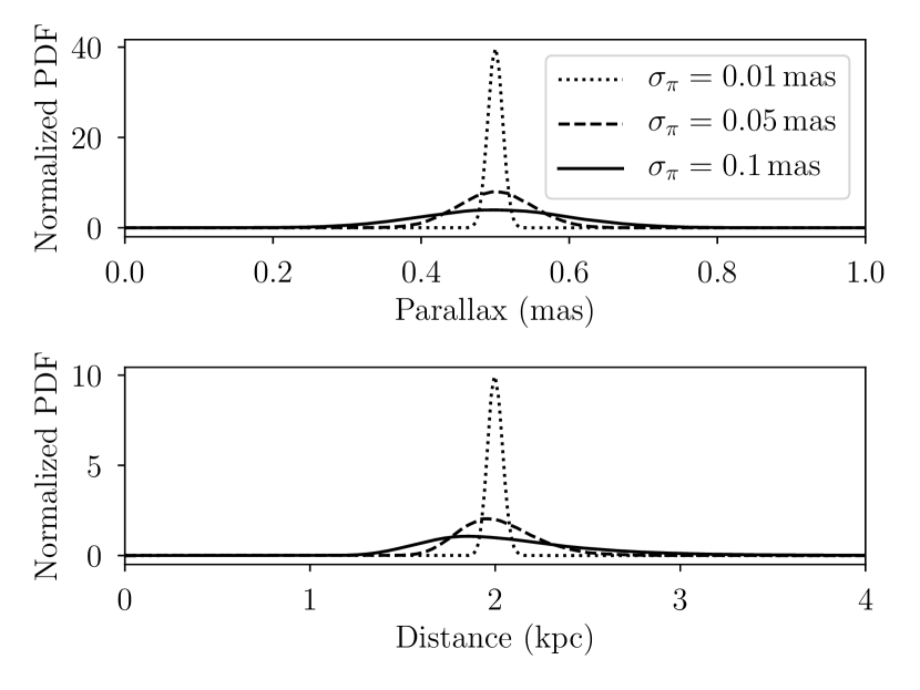
If the fractional parallax uncertainty is large, however, the shape of the parallax distance probability distribution function (PDF) is skewed. Thus the peak ($D_{P}$) and the shape of the wings change and the parallax distance uncertainty is non-symmetric around the peak (see Kovalevsky, 1998). Figure 1 shows an example of the parallax distance PDF skew for different parallax uncertainties.

Figure 1: Normalized parallax probability distribution function (PDF; top) and parallax distance PDF (bottom). The parallax in this example is $\pi=0.5\,\text{mas}$ and the parallax uncertainty is $\sigma_{\pi}=0.01\,\text{mas}$ (dotted), $0.05\,\text{mas}$ (dashed) and $0.1\,\text{mas}$ (solid). The parallax distance PDF is determined by Monte Carlo re-sampling the Gaussian parallax PDF. For large relative parallax uncertainties, the parallax distance PDF is skewed.

Figure 2: Normalized parallax distance probability distribution functions (PDFs) for four HMSFRs. The solid curve is the kernel density estimator (KDE) of the distribution; the solid vertical line is the peak of the KDE and our assigned parallax distance. The dashed vertical line is the parallax distance given by Equation 1. The vertical dotted lines span the symmetric uncertainty range in the parallax distance derived by propagating the parallax uncertainty through Equation 1. The filled region is the uncertainty range derived using the KDE (see text). Panel (a) (G049.48$-$00.36; W 51 IRS2) has the largest fractional parallax uncertainty and thus has the most skewed PDF. Panel (b) (G209.00-19.38; Orion Nebula) has the smallest fractional parallax uncertainty and has the PDF closest to a Gaussian distribution. Panel (c) (G095.29-00.93) has a typical fractional parallax uncertainty. Panel (d) (G025.70+00.04) has a large fractional parallax uncertainty. It has the largest deviation from the Monte Carlo-defined parallax distance and the parallax distance derived using Equation 1.

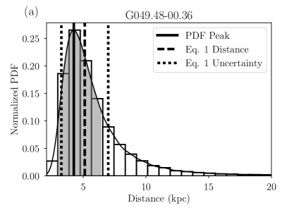
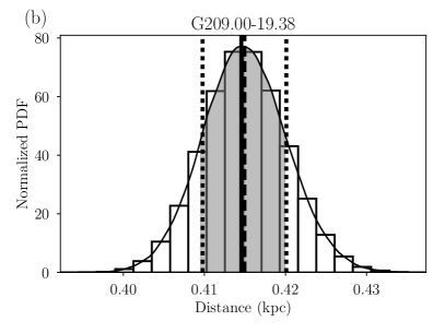
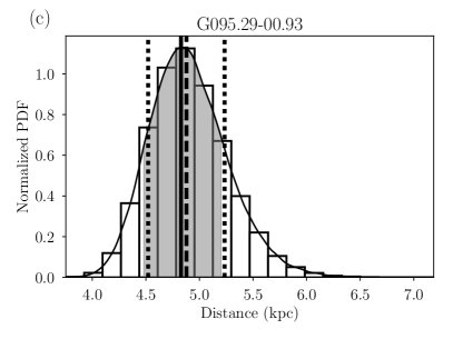
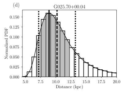
We derive a Monte Carlo parallax distance for each HMSFR by re-sampling the measured parallaxes within their uncertainties, assuming a Gaussian parallax PDF. We sample the parallax $10^{5}$ times and use Equation 1 to derive the parallax distance distribution. To approximate the parallax distance PDF, we fit a kernel density estimator (KDE) to the distribution. We use the linear combination KDE technique from Jones (1993), which is accurate even in the presence of physical boundaries such as the requirement that distances be greater than 0. The parallax distance PDFs for four sources are shown in Figure 2. The peak of the PDF (i.e. the most likely value) is the parallax distance. In every case, this distance is smaller than the distance given by Equation 1. We derive the uncertainty in the parallax distance by determining the lower and upper bounds of the PDF such that 1) the value of the PDF at both bounds is equal and 2) the integral of the normalized PDF between the bounds is equal to 0.683 (i.e., 68.3% of the total area under the PDF). This uncertainty is therefore the 68.3% confidence interval.

Figure 3: Difference (top) and fractional difference (bottom) between parallax distances derived using Equation 1, $D_{P}({\rm eq.\,1})$, and using the Monte Carlo method, $D_{P}({\rm MC})$. The solid curve is the KDE fit to the difference distribution and the solid vertical line is the median of the distribution.

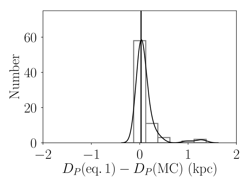
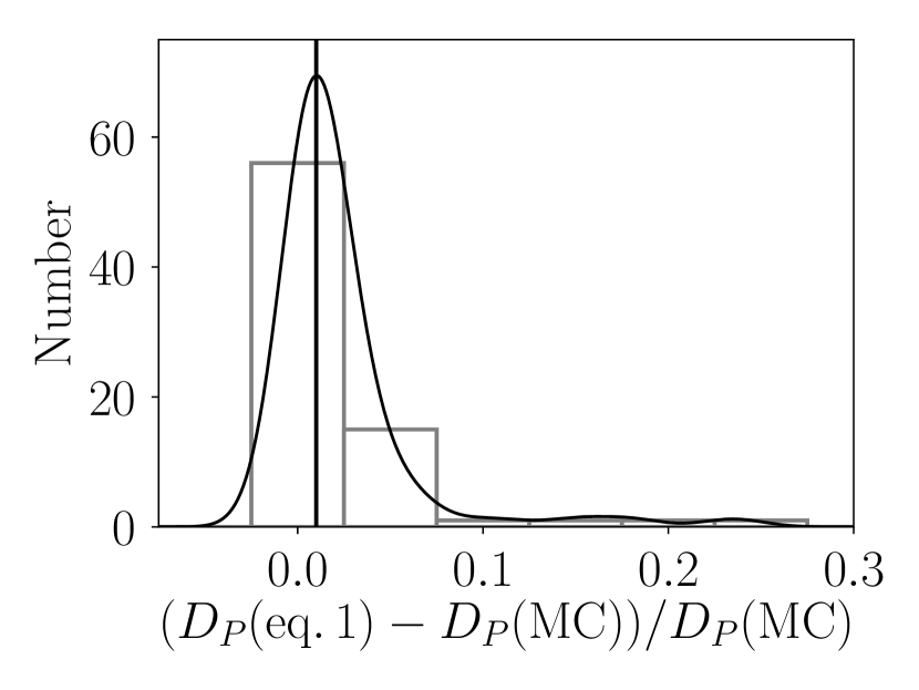
The difference between the parallax distances derived using Equation 1 and our Monte Carlo-derived parallax distances is small; the median difference is 0.03 kpc and the largest difference is 1.32 kpc for G025.70+00.04 (Figure 2, panel (d)). Figure 3 shows the distribution of parallax distance differences between these two methods for our HMSFR sample (Table 1). The majority of objects in our sample have less than $0.1\,{\rm kpc}$ difference between the Equation 1 and Monte Carlo parallax distances.

4 Kinematic Distances

A fundamental assumption of the kinematic distance method is that the chosen GRM, which gives the Galactic orbital speed, $\Theta$, at all Galactocentric radii, $R$, accurately models the Galaxy. Several different techniques have been employed to derive $\Theta(R)$, for example the tangent point method (e.g., McClure-Griffiths & Dickey, 2007) or using the full phase-space kinematics of masers associated with HMSFRs (e.g., Reid et al., 2014). The former method is only reliable in the inner-Galaxy (within the Solar orbit) whereas the latter method works across the entire Galactic disk. Reid & Dame (2016) demonstrated that both methods predict similar rotation curves in the inner-Galaxy.

Figure 4: Schematic of the kinematic distance technique. Panel (a) is the Reid et al. (2014) rotation curve. Panel (b) is a face-on view of the Galaxy with the Galactic Center located at the center and the Sun located 8.34 kpc in the direction $\theta_{\rm Az}=0^{\circ}$. The concentric circles are 4, 8, and 12 kpc in $R$ and $\theta_{\rm Az}$ is given in degrees. The solid line is a line of sight through the Galaxy with $\ell=40^{\circ}$. Panel (c) is the LSR velocity profile along this line-of-sight. An object with $V_{\rm LSR}=30\,{\rm km\,s^{-1}}$ in this direction (solid horizontal line) is an inner-Galaxy object and has two possible kinematic distances (black circles). An object with $V_{\rm LSR}=-30\,{\rm km\,s^{-1}}$ (dashed horizontal line) is an outer-Galaxy object and has only one possible kinematic distance (black square). Open circles show the location of the Sun.

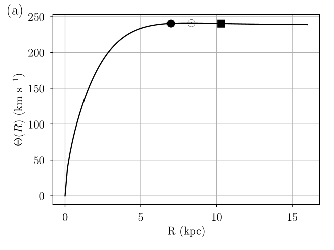
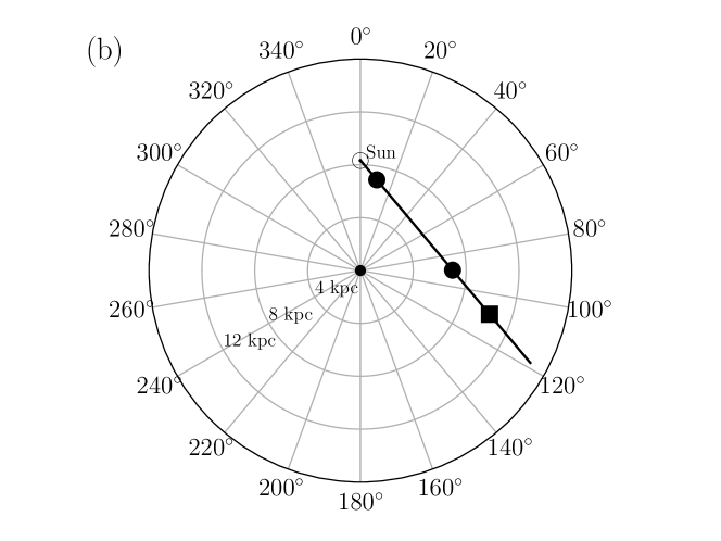
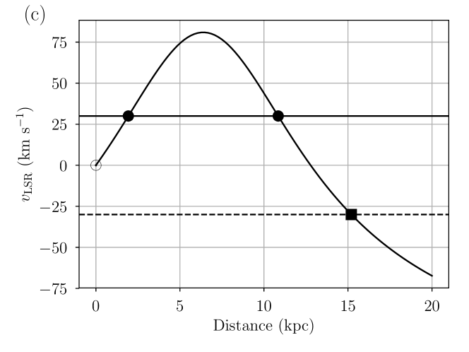
The GRM rotation curve is used to transform the Galactic longitude, Galactic latitude, distance space ($\ell,b,d$) to Galactic longitude, Galactic latitude, LSR velocity space ($\ell,b,V_{\rm LSR}$). A schematic of the kinematic distance technique is shown in Figure 4.

Many studies have shown that HMSFRs in the Milky Way do not have perfectly circular orbits; there are significant non-circular motions due to streaming in the vicinity of the Galactic bars and spiral arms (e.g., Burton, 1971; Gómez, 2006; Reid et al., 2009b, 2014). These streaming motions compromise the accuracy of kinematic distances in a complicated, uncertain way and are typically not accounted for in the derivation of kinematic distances.

A face-on view of the Anderson et al. (2012, hereafter A12) kinematic distance uncertainty model is shown in Figure 5. The A12 model includes uncertainties that stem from: (1) the variation in kinematic distances when using different GRMs; (2) the adopted values of the Solar Galactocentric Radius, $R_{0}$, and Solar circular orbit speed, $\Theta_{0}$; and, (3) including a global $7\,{\rm km\,s^{-1}}$ streaming motion uncertainty. This streaming motion uncertainty is an estimate of the true global streaming motion uncertainty which may be between 5 and $10\,{\rm km\,s^{-1}}$ (Burton, 1966). They did not, however, consider uncertainties with the GRMs or in the Solar motion parameters that define the LSR.

Figure 5: Face-on Galactic view of the A12 kinematic distance uncertainty model. The top panel is the absolute distance uncertainty and the bottom panel is the fractional distance uncertainty. The Galactic Center is located at the origin and the Sun is located 8.34 kpc in the direction $\theta_{\rm Az}=0^{\circ}$. The concentric circles are 4, 8, and 12 kpc in $R$ and $\theta_{\rm Az}$ is given in degrees. The color represents the distance uncertainty. The regions $-15^{\circ}<\ell<15^{\circ}$ and $160^{\circ}<\ell<200^{\circ}$ are masked (white) since kinematic distances are very inaccurate towards the Galactic Center and Galactic Anti-center. The black regions represent distance uncertainties greater than $\sigma_{d}=2\,{\rm kpc}$ (top) or $\sigma_{d}/d=0.5$ (bottom). The gray points are the HMSFRs in our sample.

Here we discuss three methods for calculating kinematic distances: the traditional method using the Brand & Blitz (1993) GRM (Method A), the traditional method using updated Solar motion parameters and the Reid et al. (2014) GRM (Method B), and a new Monte Carlo technique using the Reid et al. (2014) GRM (Method C).

4.1 Method A: Traditional Method, Brand & Blitz (1993) GRM

The traditional method for calculating kinematic distances uses a GRM and the measured position and LSR velocity, ($\ell,b,V_{\rm LSR}$), of an object to determine the distance(s) that correspond to the measured LSR velocity. This is typically accomplished by finding the minimum difference between the GRM LSR velocity and the measured LSR velocity (see Figure 4).

We derive the Method A kinematic distances for our sample of HMSFRs using the Brand & Blitz (1993) GRM and the uncertainty model from A12. This rotation curve and uncertainty model provide the kinematic distances and distance uncertainties listed in the WISE Catalog. We resolve the KDA by finding the kinematic distance closest to the parallax distance. If the region has an LSR velocity within $20\,{\rm km\,s^{-1}}$ of the tangent point velocity, we assign it to the tangent point. A12 used a similar tangent point strategy, but with a velocity cutoff of $10\,{\rm km\,s^{-1}}$. Our $20\,{\rm km\,s^{-1}}$ cutoff is more conservative and is more consistent with the GRM uncertainties discussed in the following sections.

4.2 Method B: Updated Solar Motion Parameters, Reid et al. (2014) GRM

In 1985, the LSR was defined by the International Astronomical Union Commission 33 as $220\,{\rm km\,s^{-1}}$ in the direction $(\ell,b)=(90^{\circ},0^{\circ})$ with a Solar non-circular motion of $20\,{\rm km\,s^{-1}}$ in the direction $\alpha=18^{\rm h}$, $\delta=+30^{\circ}$ (1900) (Kerr & Lynden-Bell, 1986). Precessing to the modern epoch (J2000), the Solar non-circular motion is defined in Galactic Cartesian coordinates as $U_{\odot}^{\rm Std}=10\,{\rm km\,s^{-1}}$ in the direction of the GC, $V_{\odot}^{\rm Std}=15\,{\rm km\,s^{-1}}$ in the direction of the Solar orbit, and $W_{\odot}^{\rm Std}=7\,{\rm km\,s^{-1}}$ in the direction of the North Galactic Pole. Since this definition was adopted, many authors have published more accurate derivations of the Solar non-circular motion parameters. For example, Reid et al. (2014) derived updated Solar motion parameters by fitting a Persic et al. (1996) universal rotation curve to the full phase-space kinematics of a sample of maser parallaxes and proper motions towards HMSFRs. The Persic et al. (1996) universal rotation curve is a physically-motivated GRM, rather than an empirical model, that includes the gravitational potential of both the disk and halo. The Persic et al. (1996) universal rotation curve is given by

$$\Theta(R)=a_{1}\left[\frac{1.97\beta x^{1.22}}{\left(x^{2}+0.78^{2}\right)^{1.43}}+\left(1-\beta\right)x^{2}\frac{1+a_{3}^{2}}{x^{2}+a_{3}^{2}}\right]^{1/2}$$ (3)

where $x=R/(a_{2}R_{0})$ and $\beta=0.72+0.44\log_{10}[(a3/1.5)^{5}]$. Here, $a_{1}$, $a_{2}$, and $a_{3}$ are the parameters fit by Reid et al. (2014). These parameters, as well as the updated Solar motion parameters fit by Reid et al. (2014), are listed in Table 2.

Table 2: Universal Rotation Curve Parameters from Reid et al. (2014)

Parameter	Value
$U_{\odot}^{\rm Rev}$ (km s-1)	10.5 $\pm\!$	1.7
$V_{\odot}^{\rm Rev}$ (km s-1)	14.4 $\pm\!$	6.8
$W_{\odot}^{\rm Rev}$ (km s-1)	8.9 $\pm\!$	0.9
$R_{0}$ (kpc)	8.31 $\pm\!$	0.16
$a_{1}$ (km s-1)	241 $\pm\!$	8
$a_{2}$	0.90 $\pm\!$	0.06
$a_{3}$	1.46 $\pm\!$	0.16

Note. — These rotation curve parameters are derived for the Persic et al. (1996) universal rotation curve (see equation 3).

To correct the LSR velocities in our sample for the updated Solar non-circular motion parameters, we first convert the measured LSR velocity to a heliocentric velocity via

$$V_{\rm helio} =V_{\rm LSR}-\left(U_{\odot}^{\rm Std}\cos\ell+V_{\odot}^{\rm Std}\sin\ell\right)\cos b$$ (4)

$$-W_{\odot}^{\rm Std}\sin b.$$

Next, we use the Reid et al. (2014) Solar motion parameters to derive the revised LSR velocity, $V_{\rm LSR}^{\rm Rev}$:

$$V_{\rm LSR}^{\rm Rev} =V_{\rm helio}+\left(U_{\odot}^{\rm Rev}\cos\ell+V_{\odot}^{\rm Rev}\sin\ell\right)\cos b$$ (5)

$$+W_{\odot}^{\rm Rev}\sin b.$$

The uncertainty in this LSR velocity ($\sigma_{V}^{\rm Rev}$) includes contributions from the uncertainty in the measured LSR velocity ($\sigma_{V}$) and the uncertainties in the Reid et al. (2014) Solar motion parameters, $\sigma_{U\odot}^{\rm Rev},\sigma_{V\odot}^{\rm Rev},\sigma_{W\odot}^{\rm Rev}$. The combined uncertainty in the revised LSR velocity is

$${\sigma_{V}^{\rm Rev}}^{2} =\sigma_{V}^{2}+\left(\sigma_{U\odot}^{\rm Rev}\cos\ell\cos b\right)^{2}+\left(\sigma_{V\odot}^{\rm Rev}\sin\ell\cos b\right)^{2}$$ (6)

$$+\left(\sigma_{W\odot}^{\rm Rev}\sin b\right)^{2}$$

For simplicity, we ignore the cross-terms between the Solar motion parameter uncertainties. Including these cross-terms would have little effect since Reid et al. (2014) finds that the magnitude of the Pearson product-moment correlation coefficients between these parameters is small, ranging between $0.011$ and $0.017$.

To compute the Method B kinematic distances to our sample of HMSFRs, we use the Reid et al. (2014) fits to the Persic et al. (1996) universal rotation curve and these revised LSR velocities. As before, we assign the near or far KDAR by determining which kinematic distance is closest to the parallax distance. If the HMSFR has an LSR velocity within $20\,{\rm km\,s^{-1}}$ of the tangent point velocity, we assign it to the tangent point distance. The Method B kinematic distance uncertainties are again determined by the A12 kinematic distance uncertainty model.

Figure 6: The Reid et al. (2014) universal rotation curve. The solid line is the nominal rotation curve using the parameters listed in Table 2. The colors represent the probability distribution function (PDF) derived by Monte Carlo re-sampling the rotation curve parameters within their uncertainties.

4.3 Method C: Monte Carlo Method, Reid et al. (2014) GRM

Here we develop a method to derive kinematic distances and their uncertainties in a more statistically robust way. With this method we re-sample all measured and derived parameters within their uncertainties and determine the probability distribution function (PDF) of kinematic distances.

We first correct the measured LSR velocities as described above. We then re-sample the revised LSR velocities from a normal distribution centered on the nominal revised LSR velocity, $V_{\rm LSR}^{\rm Rev}$, with a width $\sigma_{V}^{\rm Rev}$. The width of this distribution is the total revised LSR velocity uncertainty, which includes both the measured uncertainty and the uncertainties in the Solar motion parameters.

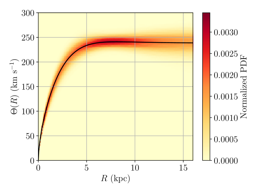
We also re-sample the Reid et al. (2014) universal Galactic rotation curve parameters, including $R_{0}$, from a normal distribution centered on the nominal values and a width equal to the uncertainty (see Equation 3 and Table 2). The variation of this re-sampled rotation curve is shown in Figure 6. Unlike A12, we do not add any additional streaming motion uncertainty into these calculations because the derivation of the Reid et al. (2014) rotation curve inherently includes uncertainties due to streaming motions.

Figure 7: Normalized probability distribution functions (PDFs) of the Method C kinematic distances derived for G032.04+00.05, $(\ell,V_{\rm LSR})=(32.0^{\circ},96.7\,\,{\rm km\,s^{-1}})$. Shown from top to bottom are the kinematic distance PDFs for: Galactocentric radius, $R$, Galactocentric radius of tangent point, $R_{\rm tan}$, near kinematic distance, $d_{\rm near}$, far kinematic distance, $d_{\rm far}$, and tangent point kinematic distance, $d_{\rm tan}$. The PDFs are determined by Monte Carlo resampling the Reid et al. (2014) rotation curve within the uncertainties in the rotation curve parameters and then deriving the kinematic distances. The solid curve is the kernel density estimation (KDE) derived using the linear combination technique from Jones (1993). The dashed vertical line is the distance derived using the “traditional” kinematic techniques whereas the solid vertical line is the peak of the KDE. The gray region is the $68.3\%$ confidence interval.

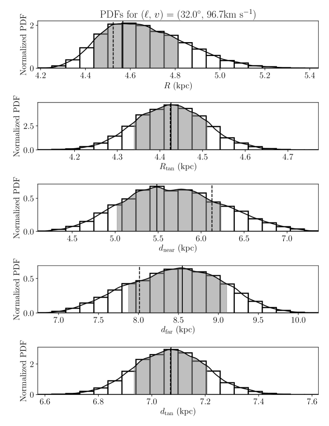
By re-sampling the above parameters $10^{5}$ times for each HMSFR, we derive the kinematic distance PDF for each object (see example for G032.04+00.05 in Figure 7). Each panel in Figure 7 represents one distance we derive: the Galactocentric radius, $R$, the Galactocentric radius of the tangent point, $R_{\rm tan}$, the near kinematic distance, $d_{\rm near}$, the far kinematic distance, $d_{\rm far}$, and the tangent point kinematic distance, $d_{\rm tan}$. The shapes of the PDFs are determined by the uncertainties in the LSR velocities, the Galactocentric radius of the Solar orbit, and the parameters of the rotation curve model.

We fit each PDF with a kernel density estimator (KDE) derived using the linear combination technique from Jones (1993). The peak of this KDE is the most probable kinematic distance, and the width and shape of the KDE describe the range of possible kinematic distances. Similar to how we defined parallax distances, we define the Method C kinematic distance as the peak of the KDE. The uncertainty in this distance is the 68.3% confidence interval.

We resolve the KDAR in the same way as in the previous two methods. If the object has a velocity in excess of the magnitude of the tangent point velocity, then the uncertainty in the tangent point distance is the formal Monte Carlo uncertainty (i.e., the 68.3% confidence interval). If the object’s velocity is smaller than the magnitude of the tangent point velocity but still within $20\,{\rm km\,s^{-1}}$, then the tangent point distance uncertainty is the total range from the near distance to the far distance. In this velocity range, traditional KDAR techniques are inaccurate and the object could be anywhere between the near and far kinematic distance (A12).

Figure 8: Face-on Galactic view of the Monte Carlo kinematic distance uncertainties. These uncertainties are not symmetric; the left panels are the uncertainty in the negative direction (toward the Sun) and the right panels are the uncertainty in the positive direction (away from the Sun). The top panels are the absolute distance uncertainties and the bottom panels are the fractional distance uncertainties. The Galactic Center is located at the origin and the Sun is located 8.34 kpc in the direction $\theta_{\rm Az}=0^{\circ}$. The concentric circles are 4, 8, and 12 kpc in $R$ and $\theta_{\rm Az}$ is given in degrees. The color represents the distance uncertainty. The regions $-15^{\circ}<\ell<15^{\circ}$ and $160^{\circ}<\ell<200^{\circ}$ are masked (white) since kinematic distances are very inaccurate towards the Galactic Center and Galactic Anti-center. The black regions represent distance uncertainties greater than $\sigma_{d}=2\,{\rm kpc}$ (top) or $\sigma_{d}/d=0.5$ (bottom). The gray points are the HMSFRs in our sample.

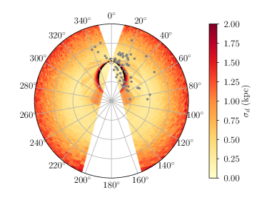
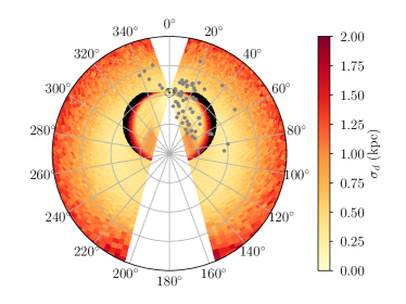
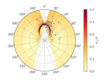
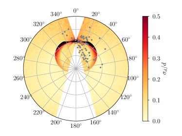
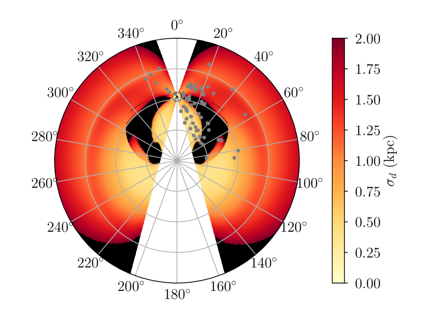
A face-on Galactic view of the Monte Carlo kinematic distance uncertainties is shown in Figure 8. To construct these maps we use the Monte Carlo technique to compute the kinematic distance and distance uncertainties in bins of $2^{\circ}$ in Galactic longitude and $2\,{\rm km\,s^{-1}}$ in velocity, with $10^{4}$ Monte Carlo samples in each bin. Since the kinematic distance uncertainties derived in this method are not symmetric, we show the uncertainties in both the positive direction (away from the Sun) and the negative direction (toward the Sun).

Table 3: Monte Carlo Parallax and Derived Kinematic Distances

Name	$D_{P}$	$D_{A}$	KDARA	$D_{B}$	KDARB	$D_{C}$	KDARC
	(kpc)	(kpc)		(kpc)		(kpc)
G015.03$-$00.67	$1.96^{+0.15}_{-0.11}$	$2.47\pm 0.60$	N	$2.33\pm 0.57$	N	$2.39^{+0.31}_{-0.41}$	N
G016.58$-$00.05	$3.54^{+0.33}_{-0.27}$	$4.60\pm 0.36$	N	$4.56\pm 0.36$	N	$4.49^{+0.50}_{-0.40}$	N
G023.00$-$00.41	$4.53^{+0.38}_{-0.35}$	$5.01\pm 0.38$	N	$4.96\pm 0.38$	N	$4.80^{+0.56}_{-0.32}$	N
G023.44$-$00.18	$5.50^{+1.25}_{-0.94}$	$5.71\pm 0.45$	N	$7.65\pm 0.60$	T	$7.65^{+1.91}_{-2.04}$	T
G023.65$-$00.12	$3.12^{+0.45}_{-0.39}$	$5.11\pm 0.39$	N	$5.07\pm 0.39$	N	$4.92^{+0.56}_{-0.36}$	N
G023.70$-$00.19	$6.05^{+0.93}_{-0.93}$	$4.68\pm 0.37$	N	$4.58\pm 0.37$	N	$4.58^{+0.45}_{-0.49}$	N
G025.70+00.04	$8.88^{+3.34}_{-1.91}$	$9.78\pm 0.46$	F	$9.50\pm 0.45$	F	$9.60^{+0.58}_{-0.62}$	F
G027.36$-$00.16	$6.79^{+3.05}_{-1.69}$	$5.52\pm 0.48$	N	$7.41\pm 0.65$	T	$5.16^{+0.75}_{-0.32}$	N
G028.86+00.06	$7.16^{+1.15}_{-0.89}$	$7.44\pm 0.83$	T	$7.30\pm 0.82$	T	$7.30^{+1.73}_{-1.80}$	T
G029.86$-$00.04	$6.02^{+0.94}_{-0.68}$	$7.37\pm 1.01$	T	$7.23\pm 1.00$	T	$7.24^{+1.46}_{-1.52}$	T
G029.95$-$00.01	$5.12^{+0.63}_{-0.46}$	$7.36\pm 0.92$	T	$7.23\pm 0.90$	T	$7.24^{+1.56}_{-1.64}$	T
G031.28+00.06	$4.05^{+0.95}_{-0.54}$	$7.26\pm 2.40$	T	$7.13\pm 2.35$	T	$7.10^{+0.91}_{-0.94}$	T
G031.58+00.07	$4.64^{+0.87}_{-0.58}$	$7.24\pm 2.59$	T	$7.10\pm 2.55$	T	$7.11^{+1.59}_{-1.66}$	T
G032.04+00.05	$5.16^{+0.24}_{-0.20}$	$7.20\pm 2.57$	T	$7.07\pm 2.52$	T	$7.07^{+1.48}_{-1.59}$	T
G033.64$-$00.22	$6.40^{+0.83}_{-0.66}$	$3.88\pm 0.43$	N	$3.65\pm 0.41$	N	$3.56^{+0.48}_{-0.35}$	N
G034.39+00.22	$1.53^{+0.15}_{-0.10}$	$3.71\pm 0.44$	N	$3.48\pm 0.41$	N	$3.37^{+0.54}_{-0.41}$	N
G035.02+00.34	$2.30^{+0.22}_{-0.22}$	$3.42\pm 0.44$	N	$3.19\pm 0.41$	N	$3.17^{+0.47}_{-0.43}$	N
G035.19$-$00.74	$2.17^{+0.24}_{-0.21}$	$2.06\pm 0.50$	N	$1.93\pm 0.47$	N	$1.87^{+0.59}_{-0.46}$	N
G035.20$-$01.73	$3.14^{+0.56}_{-0.42}$	$2.82\pm 0.46$	N	$2.62\pm 0.43$	N	$2.60^{+0.35}_{-0.35}$	N
G037.43+01.51	$1.88^{+0.07}_{-0.08}$	$2.75\pm 0.48$	N	$2.56\pm 0.45$	N	$2.50^{+0.41}_{-0.33}$	N
G043.16+00.01	$10.93^{+0.94}_{-0.79}$	$11.79\pm 0.71$	F	$11.52\pm 0.70$	F	$11.40^{+0.65}_{-0.42}$	F
G043.79$-$00.12	$6.01^{+0.19}_{-0.19}$	$3.09\pm 0.60$	N	$2.85\pm 0.55$	N	$9.16^{+0.92}_{-0.72}$	F
G043.89$-$00.78	$7.82^{+1.67}_{-1.06}$	$6.13\pm 1.12$	T	$6.01\pm 1.10$	T	$6.01^{+2.50}_{-2.40}$	T
G045.07+00.13	$7.95^{+0.37}_{-0.28}$	$6.00\pm 3.04$	T	$5.89\pm 2.98$	T	$5.91^{+1.96}_{-1.86}$	T
G045.45+00.05	$8.14^{+1.30}_{-1.16}$	$5.96\pm 1.40$	T	$5.85\pm 1.37$	T	$5.84^{+2.31}_{-2.22}$	T
G048.60+00.02	$10.65^{+0.63}_{-0.53}$	$10.02\pm 0.75$	F	$9.83\pm 0.73$	F	$9.83^{+0.58}_{-0.54}$	F
G049.19$-$00.33	$5.27^{+0.21}_{-0.20}$	$5.55\pm 2.57$	T	$5.45\pm 2.55$	T	$5.44^{+0.97}_{-0.95}$	T
G049.48$-$00.36	$4.15^{+2.40}_{-1.10}$	$5.52\pm 2.91$	T	$5.42\pm 2.91$	T	$5.43^{+1.37}_{-1.41}$	T
G049.48$-$00.38	$5.38^{+0.32}_{-0.29}$	$5.52\pm 2.85$	T	$5.42\pm 2.84$	T	$5.42^{+1.29}_{-1.15}$	T
G052.10+01.04	$3.60^{+1.27}_{-0.72}$	$5.22\pm 3.44$	T	$5.12\pm 3.45$	T	$5.15^{+1.94}_{-1.91}$	T
G059.78+00.06	$2.16^{+0.10}_{-0.10}$	$4.28\pm 4.32$	T	$4.20\pm 2.82$	T	$4.20^{+2.14}_{-2.16}$	T
G069.54$-$00.97	$2.46^{+0.08}_{-0.08}$	$2.97\pm 5.57$	T	$2.91\pm 5.87$	T	$2.91^{+2.05}_{-2.09}$	T
G074.03$-$01.71	$1.59^{+0.05}_{-0.04}$	$2.34\pm 4.15$	T	$2.29\pm 0.98$	T	$2.30^{+2.12}_{-2.05}$	T
G075.29+01.32	$9.21^{+0.47}_{-0.43}$	$10.91\pm 1.18$	F	$9.75\pm 1.02$	F	$9.61^{+1.09}_{-0.93}$	F
G075.76+00.33	$3.48^{+0.31}_{-0.26}$	$2.09\pm 0.50$	T	$2.05\pm 0.47$	T	$2.06^{+3.30}_{-2.05}$	T
G075.78+00.34	$3.73^{+0.49}_{-0.42}$	$2.09\pm 0.82$	T	$2.05\pm 0.73$	T	$2.04^{+2.54}_{-2.03}$	T
G076.38$-$00.61	$1.29^{+0.10}_{-0.08}$	$2.00\pm 0.67$	T	$1.96\pm 0.62$	T	$1.97^{+2.67}_{-1.96}$	T
G078.12+03.63	$1.63^{+0.08}_{-0.08}$	$1.75\pm 0.60$	T	$1.72\pm 0.55$	T	$1.72^{+2.85}_{-1.71}$	T
G078.88+00.70	$3.27^{+0.33}_{-0.25}$	$1.64\pm 0.54$	T	$1.61\pm 0.51$	T	$1.61^{+2.67}_{-1.60}$	T
G079.73+00.99	$1.33^{+0.14}_{-0.10}$	$1.51\pm 0.65$	T	$1.49\pm 0.59$	T	$1.48^{+2.43}_{-1.47}$	T
G079.87+01.17	$1.60^{+0.08}_{-0.06}$	$1.49\pm 0.57$	T	$1.47\pm 0.52$	T	$1.47^{+2.63}_{-1.46}$	T
G080.79$-$01.92	$1.60^{+0.13}_{-0.13}$	$1.36\pm 0.65$	T	$1.33\pm 0.58$	T	$1.33^{+2.42}_{-1.32}$	T
G080.86+00.38	$1.45^{+0.09}_{-0.08}$	$1.35\pm 0.64$	T	$1.32\pm 0.58$	T	$1.32^{+2.36}_{-1.31}$	T
G081.75+00.59	$1.49^{+0.09}_{-0.07}$	$1.22\pm 0.65$	T	$1.20\pm 0.57$	T	$1.20^{+2.33}_{-1.19}$	T
G081.87+00.78	$1.28^{+0.08}_{-0.07}$	$1.20\pm 3.65$	T	$1.18\pm 4.01$	T	$1.18^{+1.44}_{-1.17}$	T
G090.21+02.32	$0.67^{+0.02}_{-0.02}$	$2.05\pm 2.90$	F	$1.48\pm 1.49$	F	$2.23^{+0.84}_{-1.14}$	F
G092.67+03.07	$1.62^{+0.06}_{-0.05}$	$2.05\pm 2.03$	F	$1.52\pm 1.31$	F	$2.23^{+1.11}_{-1.31}$	F
G094.60$-$01.79	$3.49^{+0.43}_{-0.35}$	$6.36\pm 1.45$	F	$5.48\pm 1.23$	F	$5.30^{+1.04}_{-0.82}$	F
G095.29$-$00.93	$4.81^{+0.42}_{-0.32}$	$5.46\pm 1.44$	F	$4.68\pm 1.22$	F	$4.72^{+0.84}_{-0.99}$	F
G097.53+03.18	$7.28^{+1.07}_{-0.86}$	$9.02\pm 1.27$	F	$7.61\pm 1.07$	F	$7.28^{+1.33}_{-0.85}$	F
G100.37$-$03.57	$3.42^{+0.14}_{-0.10}$	$4.79\pm 1.42$	F	$4.06\pm 1.18$	F	$4.03^{+1.24}_{-1.24}$	F
G105.41+09.87	$0.88^{+0.06}_{-0.04}$	$1.63\pm 1.36$	F	$1.21\pm 0.94$	F	$1.22^{+0.81}_{-0.81}$	F
G107.29+05.63	$0.76^{+0.07}_{-0.06}$	$1.64\pm 1.30$	F	$1.24\pm 0.92$	F	$1.19^{+0.83}_{-0.69}$	F
G108.18+05.51	$0.75^{+0.11}_{-0.08}$	$1.60\pm 1.28$	F	$1.21\pm 0.90$	F	$1.17^{+0.74}_{-0.65}$	F
G108.20+00.58	$4.24^{+0.60}_{-0.47}$	$5.38\pm 1.37$	F	$4.48\pm 1.11$	F	$4.18^{+1.13}_{-0.68}$	F
G108.47$-$02.81	$3.23^{+0.11}_{-0.10}$	$5.89\pm 1.28$	F	$4.91\pm 1.02$	F	$4.77^{+1.01}_{-0.84}$	F
G108.59+00.49	$2.49^{+0.22}_{-0.18}$	$5.67\pm 1.32$	F	$4.72\pm 1.06$	F	$4.75^{+0.81}_{-1.05}$	F
G109.87+02.11	$0.69^{+0.04}_{-0.04}$	$1.12\pm 1.27$	F	$0.79\pm 0.81$	F	$0.81^{+0.67}_{-0.67}$	F
G111.23$-$01.23	$3.38^{+0.57}_{-0.49}$	$5.63\pm 1.27$	F	$4.67\pm 1.01$	F	$4.54^{+1.33}_{-1.13}$	F
G111.25$-$00.76	$3.37^{+0.20}_{-0.17}$	$4.58\pm 1.36$	F	$3.80\pm 1.10$	F	$3.63^{+0.99}_{-0.78}$	F
G111.54+00.77	$2.63^{+0.13}_{-0.11}$	$6.06\pm 1.14$	F	$5.01\pm 0.92$	F	$4.88^{+1.00}_{-0.92}$	F
G121.29+00.65	$0.93^{+0.03}_{-0.04}$	$2.28\pm 1.13$	F	$1.83\pm 0.88$	F	$1.86^{+0.63}_{-0.73}$	F
G122.01$-$07.08	$2.17^{+0.11}_{-0.10}$	$5.00\pm 1.18$	F	$4.10\pm 0.92$	F	$3.92^{+1.02}_{-0.73}$	F
G123.06$-$06.30	$2.77^{+0.27}_{-0.22}$	$2.91\pm 1.19$	F	$2.37\pm 0.95$	F	$2.19^{+0.84}_{-0.60}$	F
G123.06$-$06.30	$2.36^{+0.14}_{-0.12}$	$2.81\pm 1.18$	F	$2.29\pm 0.94$	F	$2.35^{+0.54}_{-0.71}$	F
G133.94+01.06	$1.95^{+0.04}_{-0.04}$	$4.93\pm 1.19$	F	$3.97\pm 0.95$	F	$3.81^{+0.96}_{-0.69}$	F
G134.62$-$02.19	$2.41^{+0.11}_{-0.10}$	$3.95\pm 1.25$	F	$3.19\pm 0.98$	F	$3.07^{+0.85}_{-0.77}$	F
G135.27+02.79	$5.97^{+0.39}_{-0.43}$	$9.37\pm 1.96$	F	$7.32\pm 1.53$	F	$7.34^{+1.26}_{-1.51}$	F
G209.00$-$19.38	$0.41^{+0.01}_{-0.01}$	$0.44\pm 0.84$	F	$0.24\pm 0.45$	F	$0.07^{+0.64}_{-0.06}$	F
G211.59+01.05	$4.39^{+0.13}_{-0.15}$	$6.49\pm 1.82$	F	$5.06\pm 1.41$	F	$4.79^{+1.45}_{-1.16}$	F
G229.57+00.15	$4.47^{+0.33}_{-0.27}$	$4.77\pm 1.11$	F	$3.83\pm 0.88$	F	$3.48^{+1.39}_{-1.09}$	F
G232.62+00.99	$1.67^{+0.11}_{-0.10}$	$2.01\pm 1.04$	F	$1.59\pm 0.79$	F	$1.52^{+0.58}_{-0.53}$	F
G236.81+01.98	$3.31^{+0.24}_{-0.18}$	$4.22\pm 1.25$	F	$3.43\pm 0.98$	F	$3.19^{+1.13}_{-0.70}$	F
G239.35$-$05.06	$1.16^{+0.09}_{-0.08}$	$2.02\pm 1.07$	F	$1.59\pm 0.81$	F	$1.62^{+0.52}_{-0.66}$	F
G240.31+00.07	$4.68^{+0.44}_{-0.49}$	$7.11\pm 1.30$	F	$5.75\pm 1.04$	F	$5.75^{+1.03}_{-1.13}$	F

5 Kinematic Distance Uncertainty

We assess the accuracy of kinematic distances by comparing the parallax and kinematic distances for each of the three kinematic distance methods. Table 3 lists the derived distances for our sample: the Monte Carlo parallax distance, $D_{P}$, the kinematic distances using each of the three methods, $D_{A}$, $D_{B}$, and $D_{C}$, and their associated KDARs: KDAR_A, KDAR_B, and KDAR_C.

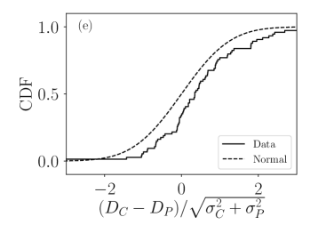
Here we investigate the differences between the parallax distances and kinematic distances and compare those differences to the kinematic and parallax distance uncertainties. For each kinematic distance method we generate six figures: (1) a histogram of the difference between the kinematic distance and the parallax distance; (2) a histogram of the fractional distance difference; (3) a scatter plot of the distance difference as a function of the parallax distance; (4) a scatter plot of the distance difference minus the median difference as a function of the parallax distance; (5) a cumulative distribution function (CDF) of the ratio of the distance difference to the uncertainty in the distance difference; and (6) a CDF of the ratio of the distance difference minus the median difference to the difference uncertainty.

The distance difference histograms reveal any systematic differences between the kinematic and parallax distances. The scatter plots uncover correlations between the distance difference and the parallax distance. Finally, the CDFs characterize the accuracy of the kinematic and parallax distance uncertainties; if the kinematic and parallax distance uncertainties are random and an accurate representation of the data, the CDF should follow a normal distribution.

Figure 9: Difference between parallax distances and Method A kinematic distances. Panel (a): histogram of distance difference. The solid curve is the KDE fit to the difference distribution and the solid vertical line is the median of the distribution. Panel (b): histogram of the fractional distance difference. Panel (c): scatter plot of distance difference as a function of parallax distance. Panel (d): scatter plot of the distance difference minus the median distance difference as a function of parallax distance. Panel (e): cumulative distribution function (CDF) of the ratio of the distance differences to the distance difference uncertainties. Panel (f): CDF of the ratio of the distance differences minus the median difference to the distance difference uncertainties. The dashed curve in Panels (e) and (f) is the expected CDF for a normal distribution centered on zero. The CDF does not go to 0 on the left nor to 1 on the right because there is at least one source beyond the limits of the abscissas.

Figure 10: Same as Figure 9 but using Method B kinematic distances.

Figure 11: Same as Figure 9 but using Method C kinematic distances.

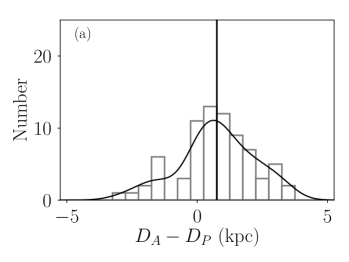
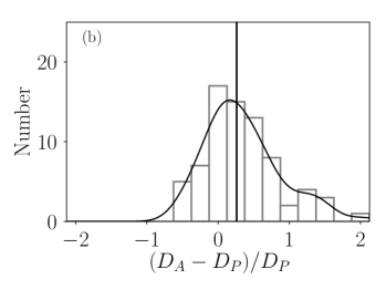
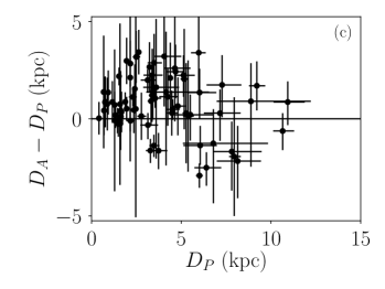
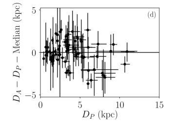
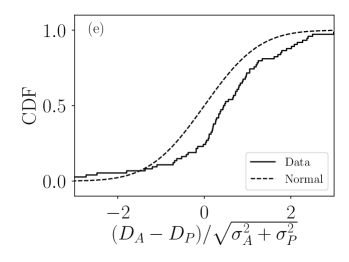
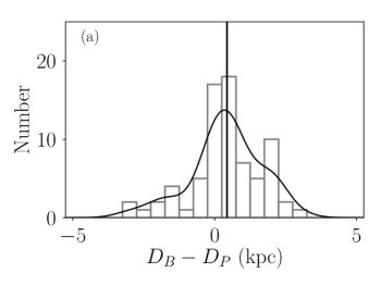
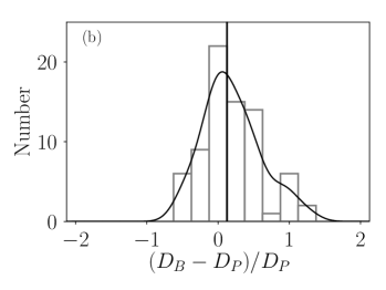
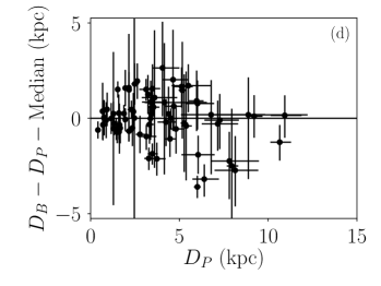
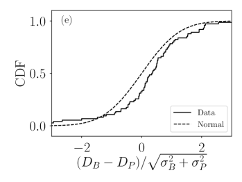
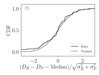
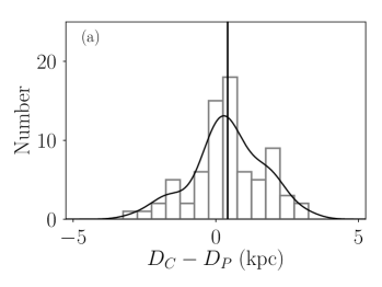
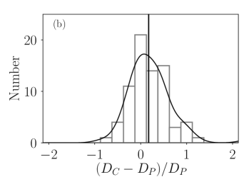
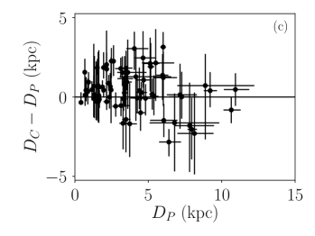
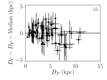
We first compare the parallax distances to the Method A kinematic distances, $D_{A}$. The distance differences are shown in Figure 9. We compute the mean, median, and standard deviation of the distance difference (i.e., $D_{A}-D_{P}$), the absolute distance difference (i.e., $|D_{A}-D_{P}|$), the fractional distance difference (i.e., $(D_{A}-D_{P})/D_{P}$), and the absolute fractional distance difference (i.e., $|D_{A}-D_{P}|/D_{P}$). These values are listed in Table 4. The fractional distance difference distribution in Panel (b) has a long tail towards larger kinematic distances.

After subtracting the median offset, the kinematic distance uncertainties from the A12 model fit the differences between the kinematic and parallax distances well. Panel (f) of Figure 9 shows that the ratio of the distance difference (minus the median difference) to the difference uncertainty follows a normal distribution, indicating that the kinematic and parallax distance uncertainties accurately represent the random errors in the distances. The K–S statistic for this distribution is $0.121$ which corresponds to a p–value of $0.203$. Panel (d), however, shows that some of the error bars are large even when the difference between the kinematic and parallax distance is small. This implies that the kinematic distance uncertainty model is over-predicting the kinematic distance uncertainties in some cases. The median Method A kinematic distance uncertainty (i.e., $\sigma_{A}/D_{A}$) is $28.0\%$.

Next, we compare the parallax distances to the Method B kinematic distances, $D_{B}$. The differences between these two distances are shown in Figure 10, and the mean, median, and standard deviation statistics are listed in Table 4. The mean and median distance differences are significantly smaller than those found using Method A. The fractional distance difference distribution is both centered closer to zero and narrower than the Method A distribution. The tail towards larger fractional differences is not nearly as long using this method.

Once again, the A12 kinematic distance uncertainty model seems to accurately represent the typical differences between the parallax and kinematic distances. The K–S statistic for the median-corrected CDF is $0.081$ with a p–value of $0.716$, thus strongly implying that the uncertainties are sampled from a normal distribution. The kinematic distance errors are, however, large for sources with kinematic distances and parallax distances in good agreement. The median Method B kinematic distance uncertainty is the same as with method A at $28.0\%$.

Finally, we compare the parallax distances to the Method C kinematic distances, $D_{C}$. The distance differences using this method are shown in Figure 11 and the mean, median, and standard deviation statistics are in Table 4. These statistics and distributions are nearly identical to those found using Method B.

The kinematic distance uncertainties derived using the Monte Carlo method (Method C) are just as accurate as those given by the A12 kinematic distance uncertainty model (Methods A and B). Panel (f) of Figure 11 shows that the kinematic distance uncertainties follow a normal distribution with a K–S statistic of $0.083$ (p–value is $0.681$). This distribution and K–S statistic are nearly the same as that of Method B, yet the distance uncertainties are not assigned based on a model but rather derived based on the data and GRM. The median Method C kinematic distance uncertainty is slightly smaller than that of Method B at $25.8\%$. More than half (56%) of the Method C kinematic distance uncertainties are smaller than the Method B uncertainties. Despite these smaller error bars, panel (f) of Figure 11 shows that these kinematic distance uncertainties fit the data just as well as the A12 model used in Method A and B.

Table 4 summarizes the aforementioned results for the three kinematic distance methods. The median absolute distance difference is nearly ${\sim}40\%$ smaller using Methods B and C, with a ${\sim}12\%$ smaller standard deviation. The median-corrected K–S statistic is about $30\%$ smaller using Methods B and C, and nearly identical between Methods B and C. This suggests that the Monte Carlo-derived kinematic distance uncertainties (Method C) are just as accurate as the A12 kinematic distance uncertainty model (Method B). The median kinematic distance uncertainty, $\sigma_{D}/D$, is the smallest using Method C.

Table 4: Distance Difference Statistics

	Method A	Method B	Method C
$D-D_{P}$ (kpc)
Median	0.75	0.43	0.42
Mean	0.74	0.40	0.42
Std. Dev.	1.42	1.24	1.23
$|D-D_{P}|$ (kpc)
Median	1.13	0.68	0.71
Mean	1.29	1.00	1.01
Std. Dev.	0.95	0.83	0.83
$(D-D_{P})/D_{P}$ (percent)
Median	26	13	17
Mean	35	20	21
Std. Dev.	52	40	46
$|D-D_{P}|/D_{P}$ (percent)
Median	33	24	26
Mean	46	34	36
Std. Dev.	43	30	36
$\sigma_{D}/D$ (percent)
Median	28.0	28.0	25.8
$(D-D_{P}-{\rm Median})/\sqrt{\sigma_{D}^{2}+\sigma_{P}^{2}}$
K–S statistic	0.121	0.081	0.083
K–S p–value	0.203	0.716	0.681

6 Kinematic Distance Ambiguity (KDA)

Thus far we resolved the KDA by assigning the kinematic distance closest to the parallax distance, or by assigning objects within $20\,{\rm km\,s^{-1}}$ of the tangent point velocity to the tangent point distance. The WISE Catalog of Galactic H ii Regions (Anderson et al., 2014) contains the KDAR for 34 of our sources determined using a variety of KDAR techniques. Here we compare our parallax-based KDARs to the WISE Catalog KDARs.

Figure 12: Difference between RRL and maser LSR velocity (top) and molecular line and maser LSR velocity (bottom). The solid curve is the KDE fit to each distribution, and the vertical line is the median.

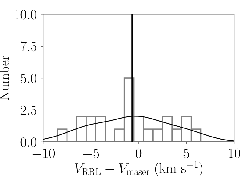
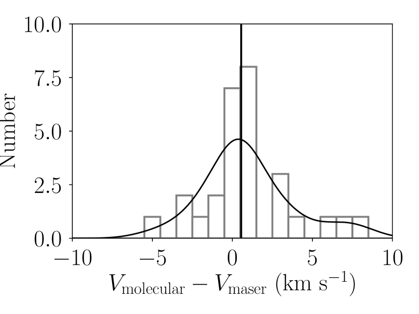
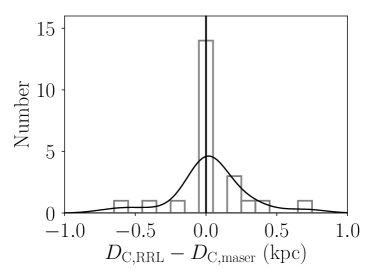
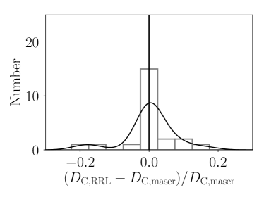
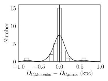
We first compare the LSR velocities of non-maser transitions in the WISE Catalog to the maser velocities from Reid et al. (2014). The WISE Catalog contains RRL velocities and/or non-maser molecular spectral line velocities for 34 HMSFRs: 6 regions with only RRL velocities, 11 regions with only molecular line velocities, and 17 regions with both. Since the RRL emission comes from the ionized gas of the HMSFR and the non-maser molecular line emission comes from molecular clouds associated with the HMSFR, the LSR velocities of these transitions need not be the same as that of the maser emission, which originates within the molecular envelope of the high mass stars. Figure 12 shows the difference between the RRL and maser velocities and the difference between the molecular line velocities and maser velocities. The median difference is $-0.70\,{\rm km\,s^{-1}}$ with a standard deviation of $3.83\,{\rm km\,s^{-1}}$ for RRL velocities and $0.55\,{\rm km\,s^{-1}}$ with a standard deviation of $2.73\,{\rm km\,s^{-1}}$ for molecular line velocities. These distributions are consistent with the expected ${\sim}10\,{\rm km\,s^{-1}}$ difference between maser spot emission region motions and bulk gas motions (e.g., Reid et al., 2009b, 2014). The difference in LSR velocities corresponds to differences in kinematic distances. The differences between the Method C kinematic distances derived using the RRL, molecular, and maser velocities are shown in Figure 13. The median difference is $0\,{\rm kpc}$ for both the RRL and maser distance difference and the molecular and maser distance difference, with standard deviations of $0.25\,{\rm kpc}$ and $0.21\,{\rm kpc}$, respectively. The maximum fractional difference is $20\%$ in both cases, which implies that the choice of LSR velocity tracer has a moderate impact on the derived kinematic distance.

Figure 13: Difference between the Method C kinematic distances derived using the RRL and maser LSR velocities (top) and molecular line and maser LSR velocities (bottom). The absolute difference is shown in the left panels and the fractional difference is shown in the right panels. The solid curve is the KDE fit to each distribution, and the vertical line is the median.

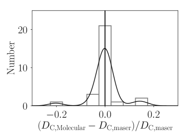
If we limit our sample to inner-Galaxy WISE Catalog objects more than $20\,{\rm km\,s^{-1}}$ from the tangent point velocity using the Reid et al. (2014) GRM, there are 9 HMSFRs. Of these, the KDAs are resolved using: H i emission/absorption and self-absorption experiments based on RRL velocities (2 objects; Anderson & Bania, 2009; Anderson et al., 2012), H i self-absorption experiments based on molecular line velocities (2 objects; Urquhart et al., 2012; Roman-Duval et al., 2009), and H₂CO absorption experiments (4 objects; Araya et al., 2002; Watson et al., 2003; Sewilo et al., 2004). One object is a visible H ii region and thus likely located at the near distance.

Based on the KDAR determined using the Method C kinematic distance method and selecting the distance closest to the parallax distance, the WISE Catalog has incorrect KDARs for 3 of our sample objects: one source (G034.39+00.22) using an H i self-absorption experiment based on RRL velocities (Anderson & Bania, 2009) and two sources (G023.70-00.19, G035.02+00.34) using H₂CO absorption experiments (Watson et al., 2003; Sewilo et al., 2004). The Anderson & Bania (2009) KDAR resolution for G034.39+00.22 was determined only with H i self-absorption techniques, and, as the authors show in that paper, H i self-absorption techniques are much less reliable than H i emission/absorption techniques. Too, this object had a low confidence H i self-absorption detection (quality factor B in that paper). The H₂CO absorption spectra for the other two sources are marginal detections. The absorption feature for (G023.70$-$00.19) is on the wing of the RRL (Sewilo et al., 2004), and the absorption feature for G035.02+00.34 is weak and ${\sim}5\,{\rm km\,s^{-1}}$ beyond the tangent point velocity (Watson et al., 2003). This sample size is too small to make any definitive conclusions about the accuracy of the KDAR techniques. Authors using the WISE Catalog KDARs should investigate the original KDAR work to assess the quality of the distance resolution.

7 Discussion

Based on the results of this analysis, we recommend the following prescription for deriving kinematic distances: (1) correct the measured LSR velocity using the Reid et al. (2014) Solar motion parameters and Equations 4 and 5; (2) use the corrected LSR velocity and the Monte Carlo method (Method C) to derive the kinematic distances and uncertainties; and (3) use only the highest quality KDARs from the WISE Catalog (if available) to resolve the kinematic distance ambiguity. The Python code we used to calculate the Monte Carlo kinematic distances is publicly available and may be utilized through an online tool (Wenger et al., 2017).

Changing the method used to derive kinematic distances may have important implications. When applying kinematic distances to Galactic morphological or metallicity structure analyses, it is important to consider the kinematic distance uncertainties and inaccuracies in the KDAR techniques. For example, Koo et al. (2017) recently re-analyzed the Leiden/Argentine/Bonn H i 21 cm line all-sky survey (Hartmann & Burton, 1997; Arnal et al., 2000; Bajaja et al., 2005; Kalberla et al., 2005) to characterize the spiral structure in the outer Galaxy. They derived kinematic distances to their H i features to produce a face-on map of the H i distribution beyond the Solar orbit. Even though there is no KDA in this part of the Galaxy, their kinematic distances will be affected by the uncertainties discussed here. Their results, determining the pitch angles of the spiral features for example, may change significantly if they use the Monte Carlo method to derive the kinematic distances of their H i features.

Monte Carlo kinematic distances will also affect the interpretation of Galactic metallicity structure. For example, Balser et al. (2015) recently discovered azimuthal variations in the radial metallicity gradient of the Milky Way inferred by the electron temperatures of Galactic H ii regions. They used the Reid et al. (2014) rotation curve to derive their kinematic distances and the A12 kinematic distance uncertainty model to assign distance uncertainties. After resampling their H ii region distances within the A12 uncertainties, they determined that the azimuthal metallicity gradient variations were statistically significant. The Balser et al. (2015) result may be affected by the results of this analysis. Not only will the kinematic distances for their sample of H ii regions change slightly, the uncertainties will change as well. These changes will affect the statistical significance of their result.

This new kinematic distance method will affect all distance estimation techniques that rely, at least in part, on kinematic distances. For example, Reid et al. (2016) used a Bayesian distance estimation method to derive the distance to HMSFRs. The priors in their method included the parallax distance (if available), the kinematic distance with equal weight given to both the near and far kinematic distance, the Galactic latitude, and a spiral arm model of the Galaxy. Instead of using a Gaussian kinematic distance PDF, future Bayesian analyses should use the full Monte Carlo kinematic distance PDF.

Figure 14: Difference between Method A and Method C kinematic distances (top) and Method B and Method C kinematic distances (bottom) as a function of LSR velocity in the direction $\ell=30^{\circ}$. The black points correspond to near kinematic distances and the red points correspond to far kinematic distances. The error bars are the combined uncertainties of both the A12 kinematic distance uncertainty model (Methods A and B) and the Method C Monte Carlo uncertainty. We exclude $20\,{\rm km\,s^{-1}}$ near the tangent point for clarity.

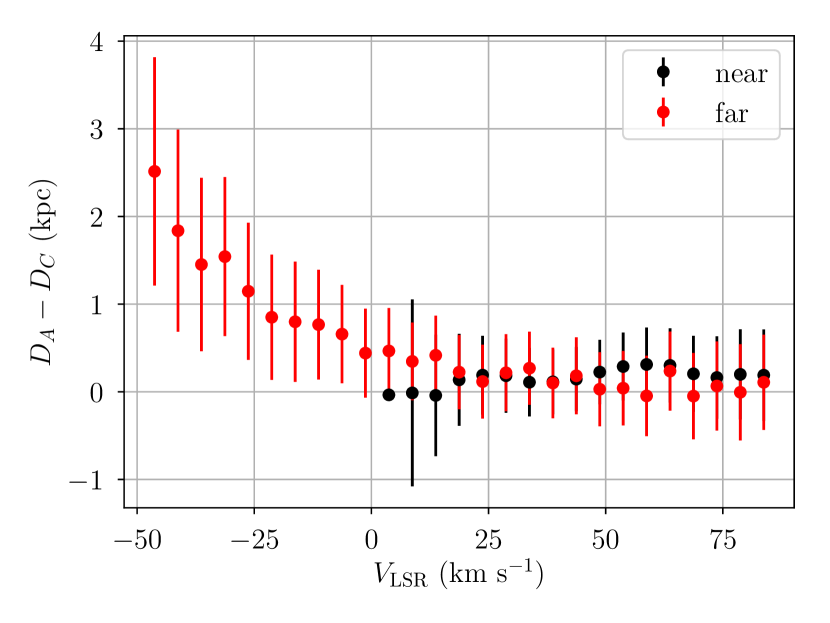
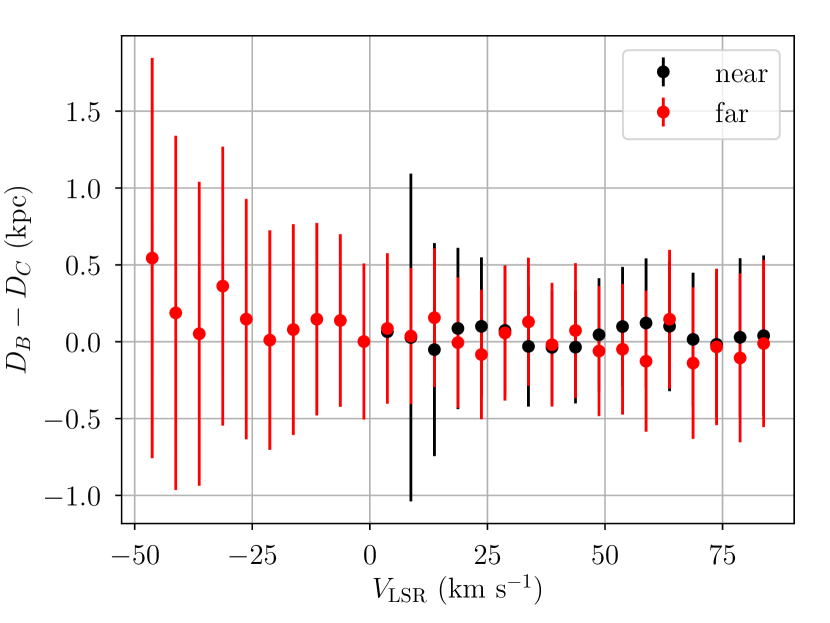
The difference between Method A and Method C kinematic distances is fairly large, whereas the difference between Method B and Method C is small. Figure 14 shows the difference between the Method A and C distances as well as the Method B and C distances for LSR velocities along $\ell=30^{\circ}$. We choose this line-of-sight because it crosses both the inner and outer Galaxy through most of the Galactic disk. The difference between Method A and C is $<0.5\,{\rm kpc}$ within the Solar orbit, and approaches $3\,{\rm kpc}$ at a distance of $20\,{\rm kpc}$. This discrepancy is caused by the variations in the GRMs used by each method. The difference between Method B and C, however, is small ($\,\lesssim\,0.5\,{\rm kpc}$) across the Galaxy since both methods use the same GRM.

Figure 15: Ratio of the Method C Monte Carlo kinematic distance uncertainty to the A12 kinematic distance uncertainty model (Methods A and B) as a function of distance in the direction $\ell=30^{\circ}$. The solid vertical line indicates a ratio of one where $\sigma_{C}=\sigma_{A,B}$. The spikes near $5\,{\rm kpc}$ and $9\,{\rm kpc}$ are at the boundaries of the “tangent point region,” defined where the LSR velocity is within $20\,{\rm km\,s^{-1}}$ of the tangent point velocity.

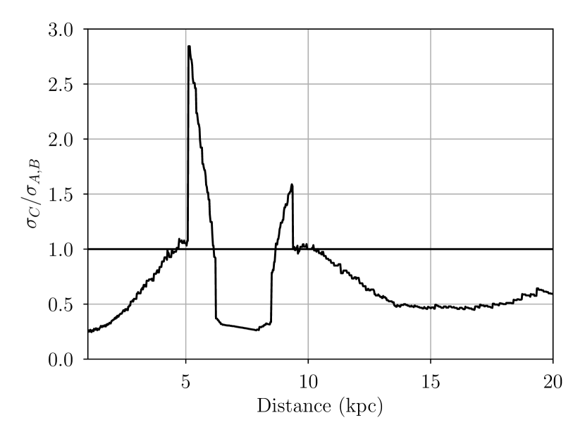
The largest distinction between the different kinematic distance methods is the magnitude of the uncertainties. In Figure 15 we show the ratio of the Method C kinematic distance uncertainty to those of Methods A and B (the A12 model) along $\ell=30^{\circ}$. Except near the tangent point, the Method C kinematic distance uncertainties are smaller than the A12 model uncertainties. At a distance of $15\,{\rm kpc}$, the Model C uncertainty is half of the A12 model uncertainty. The spikes near $5\,{\rm kpc}$ and $9\,{\rm kpc}$ are located at the boundaries of the “tangent point region” (within $20\,{\rm km\,s^{-1}}$ of the tangent point velocity). Here, the Method C kinematic distance uncertainties are much larger than the A12 model uncertainties.

Figure 16: Face-on Galactic view of the parallax distance uncertainties assuming a typical parallax uncertainty of $0.02\,\mu\text{as}$. The top panel is the absolute distance uncertainty and the bottom panel is the fractional distance uncertainty. The Galactic Center is located at the origin and the Sun is located 8.34 kpc in the direction $\theta_{\rm Az}=0^{\circ}$. The concentric circles are 4, 8, and 12 kpc in $R$ and $\theta_{\rm Az}$ is given in degrees. The color represents the distance uncertainty. The black regions represent distance uncertainties greater than $\sigma_{d}=2\,{\rm kpc}$ (top) or $\sigma_{d}/d=0.5$ (bottom). The gray points are the HMSFRs in our sample.

Figure 17: Ratio of the Method C Monte Carlo kinematic distance uncertainty to the typical parallax distance uncertainty as a function of distance in the direction $\ell=30^{\circ}$. The solid vertical line indicates a ratio of one where $\sigma_{C}=\sigma_{P}$. The spikes near $5\,{\rm kpc}$ and $9\,{\rm kpc}$ are at the boundaries of the “tangent point region,” defined where the LSR velocity is within $20\,{\rm km\,s^{-1}}$ of the tangent point velocity.

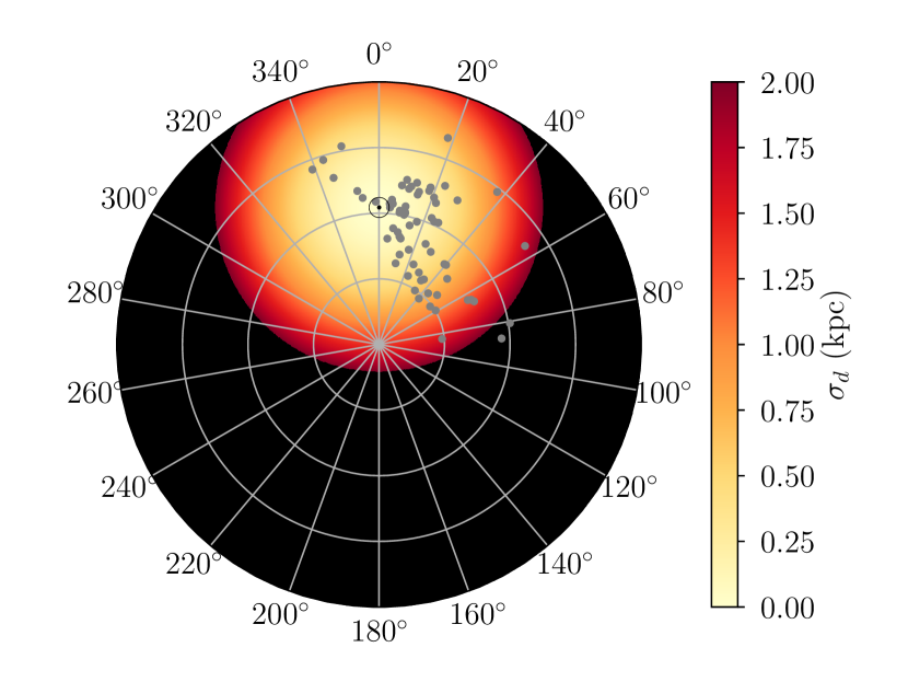
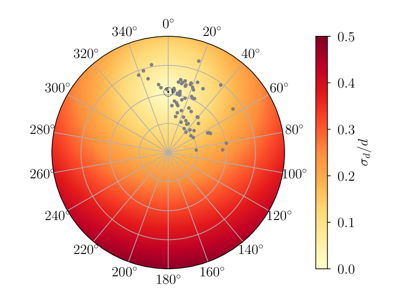
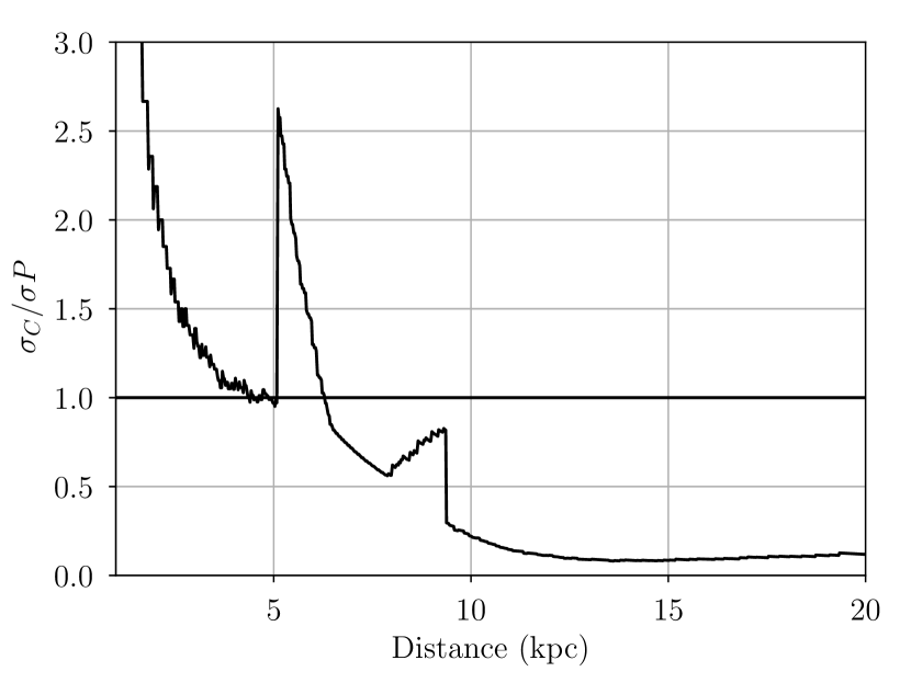
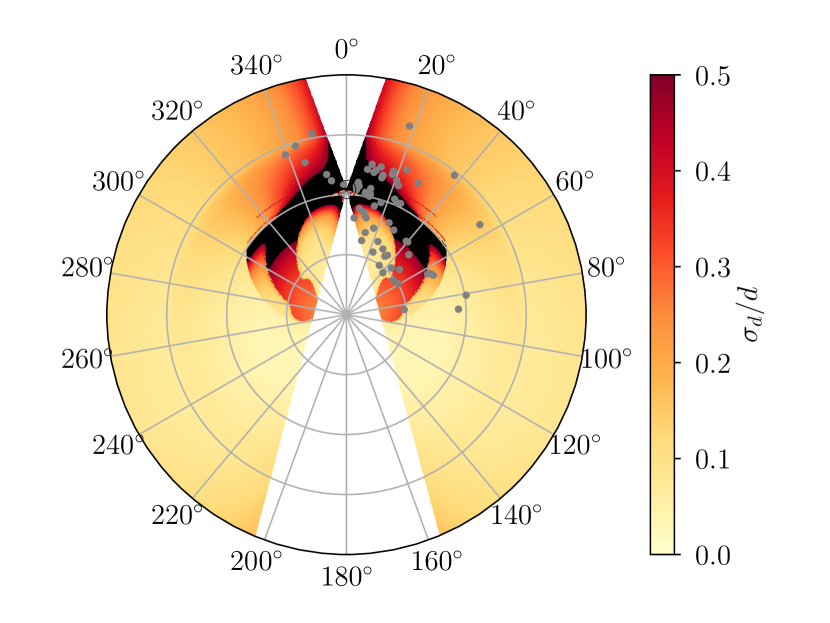
Although kinematic distances are not as accurate as parallax distances in the Solar neighborhood, their accuracy is much better in distant regions of the Milky Way. To demonstrate this point, we generate a face-on view of the typical parallax distance uncertainty in the Galaxy (Figure 16). We assume a characteristic parallax uncertainty of $0.02\,\mu\text{as}$ (Reid & Honma, 2014) which corresponds to a typical parallax distance uncertainty of $\sigma_{d}/\text{kpc}=0.02(d/\text{kpc})^{2}$. This figure uses the same color scale as the Method C Monte Carlo kinematic distance uncertainty map in Figure 8. By comparing these figures we see that large regions of Galactic quadrants I and IV ($-90^{\circ}<\ell<90^{\circ}$) have Method C kinematic distance uncertainties much smaller than the typical parallax distance uncertainties. In Figure 17 we show the ratio of the Method C kinematic distance uncertainty to the typical parallax distance uncertainty along $\ell=30^{\circ}$. Beyond the tangent point at a distance of ${\sim}8\,{\rm kpc}$, the Method C kinematic distance uncertainties are smaller than the typical parallax distance uncertainty. This ratio reaches a minimum at about $14\,{\rm kpc}$ where the Method C kinematic distance uncertainty is less than $10\%$ of the typical parallax distance uncertainty. The spikes near $5\,{\rm kpc}$ and $9\,{\rm kpc}$ are, again, located at the boundaries of the “tangent point region,” where the Method C kinematic distance uncertainties are much larger.

Figure 18: Face-on Galactic view of the typical parallax distance uncertainties converted to Galactocentric coordinates, $R$ (top) and $\theta_{\rm Az}$ (bottom). The Galactic Center is located at the origin and the Sun is located 8.34 kpc in the direction $\theta_{\rm Az}=0^{\circ}$. The concentric circles are 4, 8, and 12 kpc in $R$ and $\theta_{\rm Az}$ is given in degrees. The color represents the distance uncertainty. The black regions have uncertainties larger than the maximum value shown in the color scale. The gray points are the HMSFRs in our sample.

Figure 19: Face-on Galactic view of the Monte Carlo kinematic distance uncertainties converted to Galactocentric coordinates, $R$ (left) and $\theta_{\rm Az}$ (right). The top figures are the distance uncertainties in the negative direction while the bottom figures are the distance uncertainties in the positive direction. The Galactic Center is located at the origin and the Sun is located 8.34 kpc in the direction $\theta_{\rm Az}=0^{\circ}$. The concentric circles are 4, 8, and 12 kpc in $R$ and $\theta_{\rm Az}$ is given in degrees. The color represents the distance uncertainty. The black regions have uncertainties larger than the maximum value shown in the color scale. The regions $-15^{\circ}<\ell<15^{\circ}$ and $160^{\circ}<\ell<200^{\circ}$ are masked in white since kinematic distances are very inaccurate towards the Galactic Center and Galactic Anti-center. The gray points are the HMSFRs in our sample.

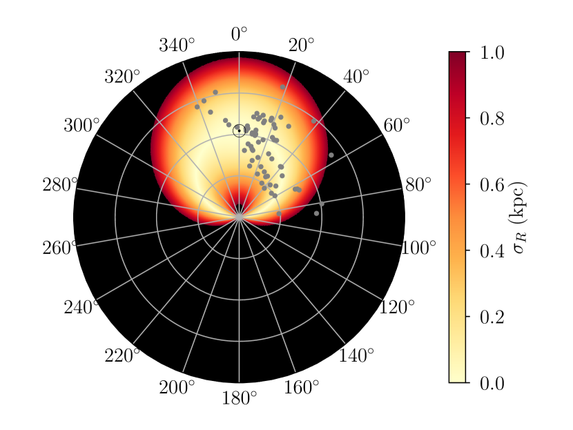
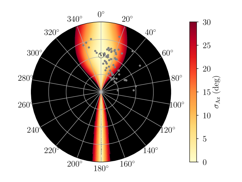
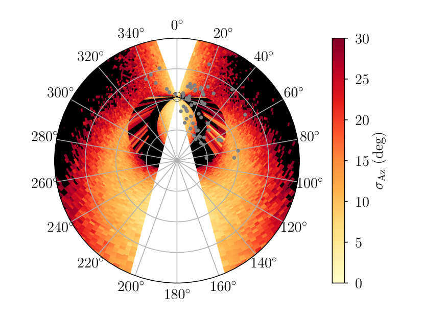
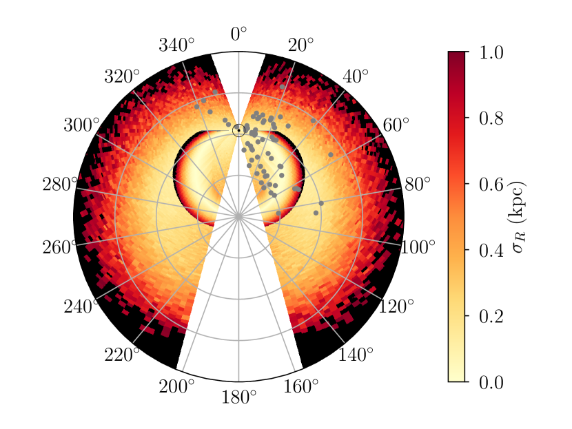
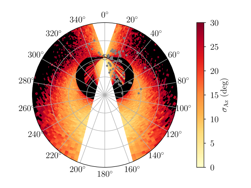
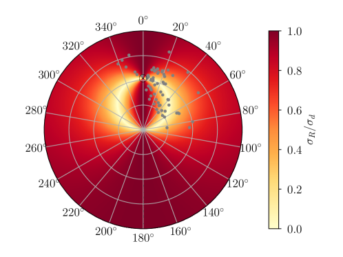
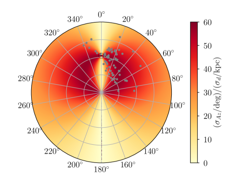
The accuracy of the Method C kinematic distances is especially apparent when we consider that Galactic structure analyses are more interested in the Galactocentric positions of structure tracers ($R,\theta_{\rm Az},z$) than the heliocentric positions ($\ell,b,d$). We derive the relationship between the distance uncertainty and uncertainties in $R$ and $\theta_{\rm Az}$ in Appendix A. Figure 18 shows the face-on uncertainties in Galactocentric position given these uncertainties in parallax distance. The same analysis using the Monte Carlo kinematic distance uncertainties is shown in Figure 19. In large regions of Galactic quadrants I and IV ($-90^{\circ}<\ell<90^{\circ}$), the Monte Carlo kinematic distances have smaller uncertainties in both $R$ and $\theta_{\rm Az}$ than the parallax distances. Kinematic distances therefore determine not only the distance of objects, but also the Galactocentric position of objects more accurately than parallax distances when the object is far from the Solar neighborhood.

Streaming motions will have a systematic effect on the accuracy of kinematic distances rather than a random effect as we have assumed in this analysis. With a much larger catalog of parallax observations of HMSFRs, we could compare kinematic and parallax distances and uncover any systematic differences. We may then be able to create a non-axisymmetric GRM that includes these non-circular motions. Such a task requires parallax observations uniformly across the entire Galactic disk.

8 Conclusions

We investigate the accuracy of kinematic distances by comparing the kinematic and parallax distances of 75 Galactic HMSFRs. We derive the kinematic distances using three different methods: the traditional method using the Brand & Blitz (1993) rotation curve and the IAU-defined Solar motion parameters (Method A), the traditional method using the Reid et al. (2014) rotation curve and their revised Solar motion parameters (Method B), and a new Monte Carlo method using the Reid et al. (2014) rotation curve and their revised Solar motion parameters (Method C). The best agreement between the kinematic and parallax distances is when we use Method C. In this case, the median absolute difference between the kinematic distances and parallax distances is $0.71\,{\rm kpc}$ with a standard deviation of $0.83\,{\rm kpc}$. The Method C kinematic distance uncertainties are smaller than those of Methods A and B for most of the Galaxy except near the tangent point. Along the line-of-sight with $\ell=30^{\circ}$, for example, the Method C kinematic distance uncertainty is $50\%$ of the Method A and B uncertainties at a distance of $15\,{\rm kpc}$. We test the accuracy of KDAR techniques using the KDARs derived in the literature for 9 of our inner-Galaxy, non-tangent point HMSFRs. The KDAR is incorrect in 3 cases when using the WISE catalog KDARs to compare the parallax distances to our Monte Carlo kinematic distances, but each of these KDARs are low-quality determinations.

We recommend a new prescription for deriving and applying kinematic distances and their uncertainties: (1) correct the measured LSR velocity using the Reid et al. (2014) Solar motion parameters and Equations 4 and 5; (2) use the corrected LSR velocity and the Monte Carlo method (Method C) to derive the kinematic distances and uncertainties; and (3) use only the highest quality KDARs from the WISE Catalog to resolve the kinematic distance ambiguity. Based on the typical parallax distance uncertainties, we show that, in a large region of Galactic quadrants I and IV ($-90^{\circ}<\ell<90^{\circ}$), both the distances and the Galactocentric positions of HMSFRs are more accurately constrained by the Method C kinematic distances than parallax distances. In the direction $\ell=30^{\circ}$, for example, the Method C kinematic distance uncertainties are smaller than the parallax distance uncertainties everywhere beyond the tangent point, reaching a minimum of $10\%$ of the parallax distance uncertainty at a distance of $14\,{\rm kpc}$. The code to derive the Method C Monte Carlo kinematic distances and kinematic distance uncertainties is publicly available and may be utilized through an on-line tool. In a future paper, we will investigate the effects of using the Monte Carlo kinematic distances on the interpretation of Galactic morphological and metallicity structure.

Appendix A Galactocentric Position Uncertainty Derivations

Here we derive the relationship between uncertainties in the distance to an object, $d$, and the uncertainties in its Galactocentric position, ($R,\theta_{\rm Az}$). For simplicity, we assume all objects are in the Galactic plane ($b=0^{\circ}$ and $z=0$).

An object’s Galactocentric radius is given by

$$R=\left(d^{2}+R_{0}^{2}-2dR_{0}\cos\ell\right)^{1/2}$$ (A1)

where $R_{0}$ is the Galactocentric radius of the Solar orbit and $\ell$ is its Galactic longitude. The uncertainty in $R$ is

$$\sigma_{R}^{2}=\sigma_{d}^{2}\left(\frac{\partial R}{\partial d}\right)^{2}+\sigma_{R_{0}}^{2}\left(\frac{\partial R}{\partial R_{0}}\right)^{2}+\sigma_{\ell}^{2}\left(\frac{\partial R}{\partial\ell}\right)^{2}$$ (A2)

where $\sigma_{R}$ is the uncertainty in $R$, $\sigma_{R_{0}}$ is the uncertainty in $R_{0}$, and $\sigma_{\ell}$ is the uncertainty in $\ell$. For simplicity we ignore cross-terms and assume $\sigma_{R_{0}}=\sigma_{\ell}=0$. The above equation then reduces to

$$\sigma_{R}^{2}=\sigma_{d}^{2}\left(\frac{\partial R}{\partial d}\right)^{2}.$$ (A3)

The partial derivative evaluates to

$$\frac{\partial R}{\partial d} =\frac{1}{2}\left(d^{2}+R_{0}^{2}-2dR_{0}\cos\ell\right)^{-1/2}\left(2d-2R_{0}\cos\ell\right)=\frac{d-R_{0}\cos\ell}{R}.$$ (A4)

The uncertainty in the Galactocentric radius of an object is thus related to the uncertainty in its distance from the Sun by

$$\sigma_{R}=\frac{\sigma_{d}}{R}|d-R_{0}\cos\ell|.$$ (A5)

This relationship is shown in the top panel of Figure 20.

An object’s Galactocentric azimuth is given by

$$\cos\theta_{\rm Az}=\frac{R^{2}+R_{0}^{2}-d^{2}}{2RR_{0}}=\frac{d^{2}+R_{0}^{2}-2dR_{0}\cos\ell+R_{0}^{2}-d^{2}}{2RR_{0}}=\frac{R_{0}-d\cos\ell}{R}.$$ (A6)

Again ignoring the $\sigma_{R_{0}}$ and $\sigma_{\ell}$ terms, the uncertainty in $\theta_{\rm Az}$ is

$$\sigma_{\rm Az}^{2}=\sigma_{d}^{2}\left(\frac{\partial\theta_{\rm Az}}{\partial d}\right)^{2}.$$ (A7)

The partial derivative evaluates to

$$\frac{\partial\theta_{\rm Az}}{\partial d} =-\frac{1}{\sqrt{1-\cos^{2}\theta_{\rm Az}}}\frac{\partial\cos\theta_{\rm Az}}{\partial d}=-\frac{1}{\sin\theta_{\rm Az}}\frac{\partial\cos\theta_{\rm Az}}{\partial d}.$$

To evaluate the derivative of $\cos\theta_{\rm Az}$, we use our expression for $R$ (Equation A1) and define functions $f(d)$ and $g(d)$ such that

$$\cos\theta_{\rm Az}=\frac{R^{2}+R_{0}^{2}-d^{2}}{2RR_{0}}=\frac{d^{2}+R_{0}^{2}-2dR_{0}\cos\ell+R_{0}^{2}-d^{2}}{2RR_{0}}=\frac{R_{0}-d\cos\ell}{R}\equiv\frac{f(d)}{g(d)}$$ (A8)

where

$$\frac{\partial f(d)}{\partial d} =\frac{\partial(R_{0}-d\cos\ell)}{\partial d}=-\cos\ell$$

$$\frac{\partial g(d)}{\partial d} =\frac{\partial R}{\partial d}=\frac{d-R_{0}\cos\ell}{R}.$$

We find

$$\frac{\partial\cos\theta_{\rm Az}}{\partial d} =-\left[\frac{-R\cos\ell-\left(R_{0}-d\cos\ell\right)\left(\frac{d-R_{0}\cos\ell}{R}\right)}{R^{2}\sin\theta_{\rm Az}}\right]$$

$$=\left[\frac{\cos\ell}{R\sin\theta_{\rm Az}}+\frac{\left(R_{0}-d\cos\ell\right)\left(d-R_{0}\cos\ell\right)}{R^{3}\sin\theta_{\rm Az}}\right].$$

The uncertainty in the Galactic azimuth is thus

$$\sigma_{\rm Az}^{2} =\sigma_{d}^{2}\left(\frac{\cos\ell}{R\sin\theta_{\rm Az}}+\frac{\left(R_{0}-d\cos\ell\right)\left(d-R_{0}\cos\ell\right)}{R^{3}\sin\theta_{\rm Az}}\right)^{2}$$

$$\sigma_{\rm Az} =\frac{\sigma_{d}}{R}\bigg{|}\csc\theta_{\rm Az}\left[\frac{\cos\ell}{\sin\theta_{\rm Az}}+\frac{\left(R_{0}-d\cos\ell\right)\left(d-R_{0}\cos\ell\right)}{R^{2}\sin\theta_{\rm Az}}\right]\bigg{|}.$$ (A9)

Rearranging, we see that the uncertainty in the Galactocentric azimuth of an object is related to the uncertainty in its distance from the Sun by

$$\sigma_{\rm Az}=\frac{\sigma_{d}}{R}\bigg{|}\frac{\cos\ell}{\sin\theta_{\rm Az}}+\frac{\left(R_{0}-d\cos\ell\right)\left(d-R_{0}\cos\ell\right)}{R^{2}\sin\theta_{\rm Az}}\bigg{|}.$$ (A10)

This relationship is shown in the bottom panel of Figure 20.

Figure 20: The relationship between the uncertainty in distance, $\sigma_{d}$, and the uncertainty in Galactocentric radius ($\sigma_{R}$, Equation A5, top) and Galactocentric azimuth ($\sigma_{\rm Az}$, Equation A10, bottom). The Galactic Center is located at the origin and the Sun is located 8.34 kpc in the direction $\theta_{\rm Az}=0^{\circ}$. The concentric circles are 4, 8, and 12 kpc in $R$ and $\theta_{\rm Az}$ is given in degrees. The color represents the uncertainty ratio. The gray points are the HMSFRs in our sample.

References

- Anderson et al. (2015) Anderson, L. D., Armentrout, W. P., Johnstone, B. M., et al. 2015, ApJS, 221, 26
- Anderson & Bania (2009) Anderson, L. D., & Bania, T. M. 2009, ApJ, 690, 706
- Anderson et al. (2014) Anderson, L. D., Bania, T. M., Balser, D. S., et al. 2014, ApJS, 212, 1
- Anderson et al. (2012) Anderson, L. D., Bania, T. M., Balser, D. S., & Rood, R. T. 2012, ApJ, 754, 62
- Ando et al. (2011) Ando, K., Nagayama, T., Omodaka, T., et al. 2011, PASJ, 63, 45
- Araya et al. (2002) Araya, E., Hofner, P., Churchwell, E., & Kurtz, S. 2002, ApJS, 138, 63
- Arnal et al. (2000) Arnal, E. M., Bajaja, E., Larrarte, J. J., Morras, R., & Pöppel, W. G. L. 2000, A&AS, 142, 35
- Asaki et al. (2010) Asaki, Y., Deguchi, S., Imai, H., et al. 2010, ApJ, 721, 267
- Astropy Collaboration et al. (2013) Astropy Collaboration, Robitaille, T. P., Tollerud, E. J., et al. 2013, A&A, 558, A33
- Bajaja et al. (2005) Bajaja, E., Arnal, E. M., Larrarte, J. J., et al. 2005, A&A, 440, 767
- Balser et al. (2015) Balser, D. S., Wenger, T. V., Anderson, L. D., & Bania, T. M. 2015, ApJ, 806, 199
- Bania et al. (2012) Bania, T. M., Anderson, L. D., & Balser, D. S. 2012, ApJ, 759, 96
- Bania et al. (2010) Bania, T. M., Anderson, L. D., Balser, D. S., & Rood, R. T. 2010, ApJ, 718, L106
- Bartkiewicz et al. (2008) Bartkiewicz, A., Brunthaler, A., Szymczak, M., van Langevelde, H. J., & Reid, M. J. 2008, A&A, 490, 787
- Bovy et al. (2014) Bovy, J., Nidever, D. L., Rix, H.-W., et al. 2014, ApJ, 790, 127
- Brand & Blitz (1993) Brand, J., & Blitz, L. 1993, A&A, 275, 67
- Brown et al. (2014) Brown, C., Dickey, J. M., Dawson, J. R., & McClure-Griffiths, N. M. 2014, ApJS, 211, 29
- Brunthaler et al. (2009) Brunthaler, A., Reid, M. J., Menten, K. M., et al. 2009, ApJ, 693, 424
- Burton (1966) Burton, W. B. 1966, Bull. Astron. Inst. Netherlands, 18, 247
- Burton (1971) —. 1971, A&A, 10, 76
- Choi et al. (2014) Choi, Y. K., Hachisuka, K., Reid, M. J., et al. 2014, ApJ, 790, 99
- Choi et al. (2008) Choi, Y. K., Hirota, T., Honma, M., et al. 2008, PASJ, 60, 1007
- Gómez (2006) Gómez, G. C. 2006, AJ, 132, 2376
- Hachisuka et al. (2009) Hachisuka, K., Brunthaler, A., Menten, K. M., et al. 2009, ApJ, 696, 1981
- Hachisuka et al. (2015) Hachisuka, K., Choi, Y. K., Reid, M. J., et al. 2015, ApJ, 800, 2
- Hachisuka et al. (2006) Hachisuka, K., Brunthaler, A., Menten, K. M., et al. 2006, ApJ, 645, 337
- Hartmann & Burton (1997) Hartmann, D., & Burton, W. B. 1997, Atlas of Galactic Neutral Hydrogen (Cambridge: Cambridge University Press), 243
- Hirota et al. (2008) Hirota, T., Ando, K., Bushimata, T., et al. 2008, PASJ, 60, 961
- Hunter (2007) Hunter, J. D. 2007, Computing In Science & Engineering, 9, 90
- Jones (1993) Jones, M. C. 1993, Statistics and Computing, 3, 135
- Kalberla et al. (2005) Kalberla, P. M. W., Burton, W. B., Hartmann, D., et al. 2005, A&A, 440, 775
- Kerr & Lynden-Bell (1986) Kerr, F. J., & Lynden-Bell, D. 1986, MNRAS, 221, 1023
- Kim et al. (2008) Kim, M. K., Hirota, T., Honma, M., et al. 2008, PASJ, 60, 991
- Kolpak et al. (2003) Kolpak, M. A., Jackson, J. M., Bania, T. M., Clemens, D. P., & Dickey, J. M. 2003, ApJ, 582, 756
- Koo et al. (2017) Koo, B.-C., Park, G., Kim, W.-T., et al. 2017, PASP, 129, 094102
- Kovalevsky (1998) Kovalevsky, J. 1998, A&A, 340, L35
- Kuchar & Bania (1994) Kuchar, T. A., & Bania, T. M. 1994, ApJ, 436, 117
- Kurayama et al. (2011) Kurayama, T., Nakagawa, A., Sawada-Satoh, S., et al. 2011, PASJ, 63, 513
- McClure-Griffiths & Dickey (2007) McClure-Griffiths, N. M., & Dickey, J. M. 2007, ApJ, 671, 427
- McKinney (2010) McKinney, W. 2010, in Proceedings of the 9th Python in Science Conference, ed. S. van der Walt & J. Millman, 51 – 56
- Menten et al. (2007) Menten, K. M., Reid, M. J., Forbrich, J., & Brunthaler, A. 2007, A&A, 474, 515
- Moellenbrock et al. (2009) Moellenbrock, G. A., Claussen, M. J., & Goss, W. M. 2009, ApJ, 694, 192
- Moisés et al. (2011) Moisés, A. P., Damineli, A., Figuerêdo, E., et al. 2011, MNRAS, 411, 705
- Moscadelli et al. (2011) Moscadelli, L., Cesaroni, R., Rioja, M. J., Dodson, R., & Reid, M. J. 2011, A&A, 526, A66
- Moscadelli et al. (2009) Moscadelli, L., Reid, M. J., Menten, K. M., et al. 2009, ApJ, 693, 406
- Nagayama et al. (2011) Nagayama, T., Omodaka, T., Nakagawa, A., et al. 2011, PASJ, 63, 23
- Oh et al. (2010) Oh, C. S., Kobayashi, H., Honma, M., et al. 2010, PASJ, 62, 101
- Persic et al. (1996) Persic, M., Salucci, P., & Stel, F. 1996, MNRAS, 281, 27
- Reid & Dame (2016) Reid, M. J., & Dame, T. M. 2016, ApJ, 832, 159
- Reid et al. (2016) Reid, M. J., Dame, T. M., Menten, K. M., & Brunthaler, A. 2016, ApJ, 823, 77
- Reid & Honma (2014) Reid, M. J., & Honma, M. 2014, ARA&A, 52, 339
- Reid et al. (2009a) Reid, M. J., Menten, K. M., Brunthaler, A., et al. 2009a, ApJ, 693, 397
- Reid et al. (2009b) Reid, M. J., Menten, K. M., Zheng, X. W., et al. 2009b, ApJ, 700, 137
- Reid et al. (2014) Reid, M. J., Menten, K. M., Brunthaler, A., et al. 2014, ApJ, 783, 130
- Roman-Duval et al. (2009) Roman-Duval, J., Jackson, J. M., Heyer, M., et al. 2009, ApJ, 699, 1153
- Rygl et al. (2010) Rygl, K. L. J., Brunthaler, A., Reid, M. J., et al. 2010, A&A, 511, A2
- Rygl et al. (2012) Rygl, K. L. J., Brunthaler, A., Sanna, A., et al. 2012, A&A, 539, A79
- Sandstrom et al. (2007) Sandstrom, K. M., Peek, J. E. G., Bower, G. C., Bolatto, A. D., & Plambeck, R. L. 2007, ApJ, 667, 1161
- Sanna et al. (2012) Sanna, A., Reid, M. J., Dame, T. M., et al. 2012, ApJ, 745, 82
- Sanna et al. (2014) Sanna, A., Reid, M. J., Menten, K. M., et al. 2014, ApJ, 781, 108
- Sato et al. (2010) Sato, M., Reid, M. J., Brunthaler, A., & Menten, K. M. 2010, ApJ, 720, 1055
- Sato et al. (2008) Sato, M., Hirota, T., Honma, M., et al. 2008, PASJ, 60, 975
- Sato et al. (2014) Sato, M., Wu, Y. W., Immer, K., et al. 2014, ApJ, 793, 72
- Sewilo et al. (2004) Sewilo, M., Watson, C., Araya, E., et al. 2004, ApJS, 154, 553
- Urquhart et al. (2012) Urquhart, J. S., Hoare, M. G., Lumsden, S. L., et al. 2012, MNRAS, 420, 1656
- van der Walt et al. (2011) van der Walt, S., Colbert, S. C., & Varoquaux, G. 2011, Computing in Science & Engineering, 13, 22
- Watson et al. (2003) Watson, C., Araya, E., Sewilo, M., et al. 2003, ApJ, 587, 714
- Wenger et al. (2017) Wenger, T., Balser, D., Anderson, L., & Bania, T. 2017, KDUtils: Kinematic Distance Utilities, Astrophysics Source Code Library, , , ascl:1712.001
- Wu et al. (2014) Wu, Y. W., Sato, M., Reid, M. J., et al. 2014, A&A, 566, A17
- Xu et al. (2011) Xu, Y., Moscadelli, L., Reid, M. J., et al. 2011, ApJ, 733, 25
- Xu et al. (2009) Xu, Y., Reid, M. J., Menten, K. M., et al. 2009, ApJ, 693, 413
- Xu et al. (2006) Xu, Y., Reid, M. J., Zheng, X. W., & Menten, K. M. 2006, Science, 311, 54
- Xu et al. (2013) Xu, Y., Li, J. J., Reid, M. J., et al. 2013, ApJ, 769, 15
- Zhang et al. (2012a) Zhang, B., Reid, M. J., Menten, K. M., & Zheng, X. W. 2012a, ApJ, 744, 23
- Zhang et al. (2012b) Zhang, B., Reid, M. J., Menten, K. M., Zheng, X. W., & Brunthaler, A. 2012b, A&A, 544, A42
- Zhang et al. (2013) Zhang, B., Reid, M. J., Menten, K. M., et al. 2013, ApJ, 775, 79
- Zhang et al. (2009) Zhang, B., Zheng, X. W., Reid, M. J., et al. 2009, ApJ, 693, 419
- Zhang et al. (2014) Zhang, B., Moscadelli, L., Sato, M., et al. 2014, ApJ, 781, 89