Slow-roll corrections in multi-field inflation: a separate universes approach

Abstract

In view of cosmological parameters being measured to ever higher precision, theoretical predictions must also be computed to an equally high level of precision. In this work we investigate the impact on such predictions of relaxing some of the simplifying assumptions often used in these computations. In particular, we investigate the importance of slow-roll corrections in the computation of multi-field inflation observables, such as the amplitude of the scalar spectrum $P_{\zeta}$, its spectral tilt $n_{s}$, the tensor-to-scalar ratio $r$ and the non-Gaussianity parameter $f_{NL}$. To this end we use the separate universes approach and $\delta N$ formalism, which allows us to consider slow-roll corrections to the non-Gaussianity of the primordial curvature perturbation as well as corrections to its two-point statistics. In the context of the $\delta N$ expansion, we divide slow-roll corrections into two categories: those associated with calculating the correlation functions of the field perturbations on the initial flat hypersurface and those associated with determining the derivatives of the e-folding number with respect to the field values on the initial flat hypersurface. Using the results of Nakamura & Stewart ’96, corrections of the first kind can be written in a compact form. Corrections of the second kind arise from using different levels of slow-roll approximation in solving for the super-horizon evolution, which in turn corresponds to using different levels of slow-roll approximation in the background equations of motion. We consider four different levels of approximation and apply the results to a few example models. The various approximations are also compared to exact numerical solutions.

1 Introduction and outline

A period of inflation in the early Universe is now widely accepted as being responsible for generating the primordial density perturbations that seed all large-scale structure (LSS) in the Universe as well as the temperature fluctuations observed in the cosmic microwave background (CMB). Constraints on the amplitude and scale dependence of the primordial spectrum are already very precise, at 68% confidence level they are given as [1]

$$\ln(10^{10}A_{s})=3.062\pm 0.029\qquad\mbox{and}\qquad n_{s}=0.968\pm 0.006.$$ (1.1)

Another key property of the spectrum is its deviation from Gaussianity. In the so-called squeezed limit this can be quantified in terms of the parameter $f_{NL}^{\rm local}$, and current constraints are still consistent with this being zero [2]:

$$f_{NL}^{{\rm local}}=0.8\pm 5.0$$ (1.2)

at the $68\%$ confidence level. While this constraint is not yet as tight as those on $A_{s}$ and $n_{s}$, future LSS observations are forecast to improve constraints on non-Gaussianity to the level $\sigma(f_{NL}^{\rm local})\sim 0.1$ [3, 4].

In addition to density perturbations, inflation is also expected to give rise to gravitational waves. At present the properties of the gravitational wave spectrum are less well constrained, with an upper limit on the amplitude essentially being given as [1, 5, 6]

$$r<0.1\,.$$ (1.3)

at the $95\%$ confidence level. However, CMB polarization observations are expected to improve this constraint to the level $\sigma(r)\sim 10^{-3}$ [7].

The high-precision nature of current and forecast constraints necessitates that theoretical predictions used to compare candidate inflation models with the data must be equally as precise, and any approximations made in deriving these predictions must therefore be carefully scrutinised. One such approximation often made is the so-called slow-roll approximation, whereby the Hubble flow parameters defined as

$$\epsilon\equiv-\frac{\dot{H}}{H^{2}}\qquad\mbox{and}\qquad\eta\equiv\frac{\dot{\epsilon}}{\epsilon H}$$ (1.4)

are assumed to be small, namely $\epsilon,\eta\ll 1$. These two requirements are very generic: the first is necessary for (quasi-)exponential inflation, while the second ensures that inflation lasts for long enough. In the case of single-field inflation, on making an expansion in the two parameters $\epsilon$ and $\eta$ we find that the leading-order expression for $n_{s}$ is given as

$$n_{s}-1=-2\epsilon_{k}-\eta_{k},$$ (1.5)

where the subscript $k$ denotes that the quantities should be evaluated at the time at which the scale under consideration, $k$, left the horizon during inflation. Barring a cancellation between the two terms on the right hand side of (1.5), from the observed value of $n_{s}$ given in (1.1) we conclude that $\epsilon,\eta\lesssim\mathcal{O}(10^{-2})$. As such, in the case of single-field inflation we see that any slow-roll corrections of order $\epsilon$ or $\eta$ will likely represent percent-level corrections, and should thus be included if we desire percent-level precision in our theoretical predictions.

While current observations are perfectly consistent with single-field inflation, in the context of high-energy unifying theories one naively expects the presence of many fields. It is thus important that we are able to precisely determine the predictions of multi-field inflation models in order that they can be constrained using current and future data. Perhaps of particular interest in the context of multi-field inflation is the possibility of obtaining an observably large non-Gaussianity. In the case of single-field inflation it is known that the three-point function in the squeezed limit is unobservably small [8]. This suggests that if a non-negligible three-point function were to be observed then this would be a strong indication of the presence of multiple fields during inflation. Even if not observed, however, it is still important to determine what the implications of this are for multi-field models of inflation. Indeed, while it is possible to obtain a large non-Gaussianity in such models, it is by no means a generic prediction. When considering slow-roll corrections in multi-field inflation the situation is somewhat more complicated than in the single-field case. In addition to assuming $\epsilon,\eta\ll 1$, the slow-roll approximation is often taken to imply the smallness of a larger set of expansion parameters that we label $\eta_{IJ}$, with $I,J=1,...,M$ and $M$ being the number of fields (see Section 2 for details). One then finds that observational constraints on $n_{s}$ do not require all components of $\eta_{IJ}$ to be $\lesssim\mathcal{O}(10^{-2})$, such that slow-roll corrections of order $\eta_{IJ}$ may represent larger-than-percent-level corrections. If this is the case, the inclusion of next-to-leading order corrections will be crucial, and it is plausible that next-to-next-to-leading order corrections may also become important. Indeed, slow-roll corrections to the two-point statistics of scalar and tensor perturbations in multi-field inflation models have already been considered in the literature [9, 10], and in some cases corrections were shown to be on the order of $20\%$.

In this paper we revisit the issue of slow-roll corrections in multi-field inflation. In particular, we are interested in the slow-roll corrections to predictions for the curvature perturbation on constant density slices, $\zeta$, and quantities related to its correlation functions. Our analysis makes use of the separate universes approach and $\delta N$ formalism, which allows us to consider slow-roll corrections to the non-Gaussianity of $\zeta$ as well as corrections to its two-point statistics. As discussed above, precise predictions for the non-Gaussianity will be key in constraining multi-field models of inflation with current and future data. The paper is structured as follows. In Section 2 we introduce the class of models under consideration and present the relevant background field equations. The slow-roll approximation and associated expansion parameters are also introduced, and the background equations of motion are expanded up to next-to-leading order in the slow-roll expansion, with details of the derivation being given in Appendix A. In Section 3 we review the separate universes approach and $\delta N$ formalism on which our analysis is based. Rather than using a finite-difference method, as is often used, our method is based on the transport techniques introduced and developed in [11, 12, 13, 14, 15, 16, 17]. In this section we outline how these techniques can be applied under various levels of slow-roll approximation. In Section 4 we turn to the correlation functions of $\zeta$ as given in terms of the correlation functions of field perturbations on an initial flat slice at horizon crossing. We find that slow-roll corrections arising from slow-roll corrections to the initial field perturbations can be expressed in a compact form and in terms of quantities that in principle are observable. In Section 5 we apply the results of the earlier sections to a few example models, focussing on a comparison between the various levels of slow-roll approximation. We finally summarise our results in Section 6. In this work we use the geometrized units $c=\hbar=M_{\mathrm{Pl}}=1$, where $M_{\mathrm{Pl}}=\left(\hbar c/8\pi G\right)^{-1/2}$ is the reduced Planck mass.

2 Background dynamics and the slow-roll approximation

We consider the class of multi-field models of inflation with an action

$$S=\int d^{4}x\sqrt{-g}\left(\frac{R}{2}-\frac{1}{2}\delta_{IJ}g^{\mu\nu}\partial_{\mu}\phi^{I}\partial_{\nu}\phi^{J}-V(\vec{\phi})\right),$$ (2.1)

where $R$ is the Ricci scalar associated with the spacetime metric $g_{\mu\nu}$, $g$ is the determinant of $g_{\mu\nu}$, $\phi^{I},\,I=1,...,M$ are $M$ scalar fields and we have used the notation $\vec{\phi}=\left(\phi^{1},\ldots,\phi^{M}\right)$. $V(\vec{\phi})$ in the above action is some $\phi^{I}$-dependent potential. Note that we take the metric in field space to be Euclidean, so the distinction between upper and lower indices as in $\phi^{I}$ and $\phi_{I}$ is immaterial. We will use both of the notations interchangeably and summation is implied over repeated indices, unless stated otherwise.

At background level we take the metric $g_{\mu\nu}$ to be of the Friedmann-Lemaitre-Robertson-Walker (FLRW) type, i.e. $g_{\mu\nu}={\rm diag}\left(-1,a^{2},a^{2},a^{2}\right)$. The dynamics is then fully determined by the equations of motion for the $M$ scalar fields and the Friedmann equation, which are given as

$$\ddot{\phi}_{I}+3H\dot{\phi}_{I}+V_{,I}=0,$$ (2.2)

$$3H^{2}=\rho=\frac{1}{2}\dot{\phi}_{I}\dot{\phi}_{I}+V,$$ (2.3)

where $H=\dot{a}/a$, $\rho$ is the total energy density of the scalar fields and we have used the notation $V_{,I}\equiv\partial V/\partial\phi_{I}$. Taking the time derivative of (2.3) and using (2.2) we are able to find an expression for $\epsilon$ as defined in (1.4), which can in turn be used to determine $\eta$. The resulting expressions are given as

$$\epsilon=\frac{1}{2}\frac{\dot{\phi}_{I}\dot{\phi}_{I}}{H^{2}},\qquad\eta=2\frac{\ddot{\phi}_{I}\dot{\phi}_{I}}{H\dot{\phi}_{J}\dot{\phi}_{J}}+2\epsilon.$$ (2.4)

For the purpose of this work it is convenient to use the e-folding number $N$, rather than $t$, as the time parameter, with $N$ being defined as

$$N\equiv\ln\left(\frac{a_{\mathrm{f}}}{a_{\mathrm{i}}}\right)=\intop_{t_{\mathrm{i}}}^{t_{\mathrm{f}}}H\mathrm{d}t,$$ (2.5)

where the indices ‘$\mathrm{i}$’ and ‘$\mathrm{f}$’ denote initial and final values. In terms of $N$, eqs. (2.2), (2.3) and (2.4) take the form

$$\phi_{I}^{\prime\prime}+\left(3-\epsilon\right)\left(\phi_{I}^{\prime}+\frac{V_{,I}}{V}\right)=0,$$ (2.6)

$$H^{2}=\frac{V}{3-\epsilon}=\frac{\rho}{3},$$ (2.7)

$$\epsilon=\frac{1}{2}\phi_{I}^{\prime}\phi_{I}^{\prime},\qquad\eta=2\frac{\phi^{\prime\prime}_{I}\phi^{\prime}_{I}}{\phi^{\prime}_{J}\phi^{\prime}_{J}}$$ (2.8)

where a prime denotes a derivative with respect to $N$, e.g. $\phi_{I}^{\prime}\equiv\mathrm{d}\phi_{I}/\mathrm{d}N$.

As discussed in the introduction, in the context of inflation one often makes the so-called slow-roll approximation. At the most fundamental level this approximation corresponds to assuming $\epsilon,\eta\ll 1$, which ensures that we obtain quasi-exponential inflation that lasts for long enough. In both the single- and multi-field cases the assumption $\epsilon\ll 1$ allows us to approximate the Friedmann equation (2.7) as

$$H^{2}\simeq\frac{V}{3}\equiv\frac{\rho^{(0)}}{3}\equiv\left.H^{(0)}\right.^{2}.$$ (2.9)

In the single-field case, we see from (2.4) and (2.8) that the requirement $\eta\ll 1$ is equivalent to the requirement $\ddot{\phi}/(H\dot{\phi})\ll 1$, or $\phi^{\prime\prime}/\phi^{\prime}\ll 1$, which allows us to approximate (2.6) as

$$\phi^{\prime}+\frac{V_{,\phi}}{V}=0.$$ (2.10)

We thus find that the slow-roll approximation is equivalent to assuming that an attractor regime has been reached, in which the field velocity is no longer an independent degree of freedom but is given as a function of the field value [18]. In the multi-field case, however, the situation is more complicated, as the condition $\eta\ll 1$ only constrains the component of $\phi^{\prime\prime}_{I}$ that lies along the background trajectory, i.e. it does not necessarily imply $|\phi^{\prime\prime}_{I}/\phi^{\prime}_{I}|\ll 1$ (or equivalently $|\ddot{\phi}_{I}/(H\dot{\phi}_{I})|\ll 1$) for all $I$ (note that there is no summation over $I$ in these expressions). Nevertheless, by the Cauchy-Schwarz inequality, the constraint $\eta\ll 1$ will be satisfied if we assume that the magnitude of the field acceleration vector is smaller than the magnitude of the field velocity vector, namely $|\vec{\phi}^{\prime\prime}|/|\vec{\phi}^{\prime}|\ll 1$. If we then further assume that $\phi^{\prime}_{I}\sim\mathcal{O}(|\vec{\phi}^{\prime}|)$ for all $I$ – that is, we assume the field basis is not aligned in such a way that some of the field velocity components vanish or are considerably smaller than $|\vec{\phi}^{\prime}|$ – then we can take the slow-roll approximation to mean that $\phi^{\prime\prime}_{I}/\phi^{\prime}_{I}\ll 1$ for all $I$, such that (2.6) can be approximated as

$$\phi_{I}^{\prime}+\frac{V_{,I}}{V}=0.$$ (2.11)

In this case, we again find ourselves in an attractor regime where all field velocities are given as functions of the field positions. For later convenience we rewrite (2.11) as

$$\phi_{I}^{\prime} \simeq U_{,I}^{\left(0\right)},\qquad\mbox{where}\qquad U^{(0)}=-\ln V.$$ (2.12)

Using (2.12) we are then able to derive consistency conditions for the first and second derivatives of the potential. Explicitly, the conditions $\epsilon,\eta\ll 1$ become

$$\epsilon\simeq\frac{1}{2}\frac{V_{,I}V_{,I}}{V^{2}}\equiv\epsilon^{(0)}\ll 1,$$ (2.13)

$$\eta\simeq 2\frac{U^{(0)}_{,I}U^{(0)}_{,IJ}U^{(0)}_{,J}}{U^{(0)}_{,K}U^{(0)}_{,K}}=4\epsilon^{(0)}-\frac{1}{\epsilon^{(0)}}\frac{V_{,JK}V_{,J}V_{,K}}{V^{3}}\equiv\eta^{(0)}\ll 1.$$ (2.14)

The more stringent constraint $|\vec{\phi}^{\prime\prime}|/|\vec{\phi}^{\prime}|\ll 1$ reads

$$4\left(\epsilon^{(0)}\right)^{2}-2\frac{V_{,I}V_{,IJ}V_{,J}}{V^{3}}+\frac{V_{,I}V_{,IJ}V_{,JK}V_{,K}}{V^{2}V_{,L}V_{,L}}\ll 1.$$ (2.15)

Given that $\epsilon^{(0)}\ll 1$, the requirement $\eta\ll 1$ gives us the condition $V_{,J}V_{,JK}V_{,K}/V^{3}\ll\epsilon^{(0)}$. This in turn means that the second term in eq. (2.15) is negligible, such that the final constraint reduces to $V_{,I}V_{,IJ}V_{,JK}V_{,K}/(V^{2}V_{,L}V_{,L})\ll 1$. Introducing the notation

$$\eta_{IJ}=\frac{V_{,IJ}}{V},$$ (2.16)

both of the constraints on the second derivatives of $V$ can be satisfied if the eigenvalues of $\eta_{IJ}$ are small. This in turn will be the case if we assume

$$\eta_{IJ}\ll 1,$$ (2.17)

for all $I$ and $J$. The conditions $\epsilon^{(0)},\eta_{IJ}\ll 1$ thus constitute the slow-roll assumptions that we will make in this paper.

While (2.12) represents the lowest-order slow-roll equations of motion, in this paper we will be interested in considering next-to-leading order corrections, and we thus require the equations of motion valid to next-to-leading order in the slow-roll approximation. Details of how these can be calculated are given in Appendix A, but the final result can be written in a form almost identical to (2.12) as

$$\phi_{I}^{\prime} \simeq U_{,I}^{\left(1\right)},$$ (2.18)

with

$$U^{\left(1\right)}\equiv U^{\left(0\right)}-\frac{1}{6}U_{,I}^{\left(0\right)}U_{,I}^{\left(0\right)}.$$ (2.19)

The Friedmann equation at next-to-leading order is given as

$$H^{2}\simeq\frac{V}{3-\epsilon^{(0)}}\equiv\frac{\rho^{(1)}}{3}\equiv\left.H^{(1)}\right.^{2}\simeq\frac{V}{3}\left(1+\frac{\epsilon^{(0)}}{3}\right),$$ (2.20)

and the next-to-leading order expressions for $\epsilon$ and $\eta$, denoted $\epsilon^{(1)}$ and $\eta^{(1)}$ respectively, can be determined by substituting (2.18) into the full expressions (2.8).

Before moving on, it will turn out to be convenient later on to re-express the full equations of motion (2.6) in a more compact form that mirrors the form of eqs. (2.12) and (2.18). In order to do so, we introduce the notation

$$\varphi_{i}\equiv\left(\phi_{I},\phi_{I}^{\prime}\right),$$ (2.21)

where the index $i$ runs from $1$ to $2M$. This allows us to write (2.6) as

$$\varphi^{\prime}_{i}=\mathbb{U}_{i},$$ (2.22)

where

$$\mathbb{U}_{i}\equiv\phi_{i}^{\prime}\qquad \text{ for }1\leq i\leq M$$ (2.23)

$$\mathbb{U}_{i}\equiv-\left(3-\epsilon\right)\left(\phi_{i-M}^{\prime}+\frac{V_{,i-M}}{V}\right)\qquad \text{ for }M+1\leq i\leq 2M.$$ (2.24)

3 The curvature perturbation $\zeta$

In this section we outline the method we use to determine the curvature perturbation on constant density slices, $\zeta$, which is based on the separate universes approach and $\delta N$ formalism [19, 20, 21, 22, 23, 24, 25].

3.1 The separate universes approach and $\delta N$ formula

The separate universes approach corresponds to the lowest-order approximation in a gradient expansion [22, 23]. First, one performs a smoothing of the Universe on some scale $L$ that is larger than the Hubble scale $1/H$, namely $LH\gg 1$. Associating the small parameter $\xi=1/(LH)$ with spatial gradients, one then expands the relevant dynamical equations in powers of $\xi$, and to the lowest order neglects terms of order $\mathcal{O}(\xi^{2})$ or greater. Consequently, one finds that individual $L$-sized patches behave as separate universes, evolving independently and according to the background field equations. On scales larger than $L$, the differences between neighbouring patches simply result from differences in initial conditions. If we are interested in the comoving scale with wavenumber $k$ then we have $\xi=k/(aH)$. During inflation this parameter will be decreasing exponentially with time, and the separate universes approach will be applicable after the Horizon-crossing time, which is defined as the time at which $k=aH$.

Ultimately we are interested in computing the curvature perturbation on constant density slices, $\zeta$, and in the context of the separate universes approach it can be shown that $\zeta$ is given by the number of e-foldings of expansion between a flat and constant density slice, $\delta N$. To see why this is, let us consider the spatial metric, which can be written as

$$g_{ij}\left(t,\bm{x}\right)=a^{2}\left(t\right)\mathrm{e}^{2\psi\left(t,\bm{x}\right)}\gamma_{ij}\left(\bm{x}\right),$$ (3.1)

where $a(t)$ is the fiducial background scale factor, $\psi(t,\bm{x})$ is the curvature perturbation and $\gamma_{ij}$, satisfying $\mathrm{det}\gamma_{ij}=1$, contains gravitational waves. Here we follow [23] and fix the threading such that the scalar and vector parts of $\gamma_{ij}$ are set to zero. Note that the fiducial background universe can be associated with some given location $\bm{x}_{0}$, namely $g_{ij}(t,\bm{x}_{0})=a^{2}(t)\delta_{ij}$. We can then consider $\tilde{a}(t,\bm{x})\equiv a(t)\,{\rm{e}}^{\psi(t,\bm{x})}$ as the effective scale factor at a given location $\bm{x}$, and the associated e-folding number is given as

$$\tilde{N}(t_{\rm f},t_{\rm i},\bm{x})=\ln\left(\frac{\tilde{a}(t_{\rm f},\bm{x})}{\tilde{a}(t_{\rm i},\bm{x})}\right)=\psi(t_{\rm f},\bm{x})-\psi(t_{\rm i},\bm{x})+N(t_{\rm f},t_{\rm i}).$$ (3.2)

If we were to consider flat slices, where $\psi(t,\bm{x})=0$, then we see that the scale factor reduces to that of the fiducial background, namely $\tilde{a}(t,\bm{x})=a(t)$, and correspondingly the e-folding number remains unperturbed, i.e. $\tilde{N}(t_{\rm f},t_{\rm i},\bm{x})=N(t_{\rm f},t_{\rm i})$. On the other hand, if we were to consider moving between a flat slice at $t_{\rm i}$, with $\psi(t_{\rm i},\bm{x})=0$ such that $\tilde{a}(t_{\rm i},\bm{x})=a(t_{\rm i})$, and a constant density slice at $t_{\rm f}$, on which $\delta\rho(t_{\rm f},\bm{x})=0$ and $\psi(t_{\rm f},\bm{x})=\zeta(t_{\rm f},\bm{x})$ such that $\tilde{a}(t_{\rm f},\bm{x})=a(t_{\rm f})\rm e^{\zeta(t_{\rm f},\bm{x})}$, then we find

$$\zeta(t_{\rm f},\bm{x})=\delta N(t_{\rm f},\bm{x})=\tilde{N}(t_{\rm f},t_{\rm i},\bm{x})-N(t_{\rm f},t_{\rm i}).$$ (3.3)

Note that the left-hand side of the above equation is independent of $t_{\rm i}$, i.e. it is independent of when we take our initial flat slice. This reflects the fact that the number of e-foldings between any two flat slices is homogeneous, and therefore does not contribute to $\delta N(t,\bm{x})$.

If we consider the case $t_{\rm i}=t_{\rm f}-\delta t$, then $\delta N(t,\bm{x})$ given in (3.3) corresponds to the perturbation in the number of e-foldings that results from making a gauge transformation between the flat and constant-density slices at the final time $t_{f}$. In this case we can derive a simple relation between $\delta N(t,\bm{x})$ and the density perturbation on the flat hypersurface. As the e-folding number is unperturbed on flat hypersurfaces, it is useful to use this as a time parameter. We can then decompose the density on the flat hypersurface as $\rho(N,\bm{x})=\rho(N)+\delta\rho(N,\bm{x})$, where $\rho(N)$ is the density of the fiducial background trajectory associated with the location $\bm{x}_{0}$, namely $\rho(N,\bm{x}_{0})=\rho(N)$. Next we consider the shift in $N$ required at each location $\bm{x}$ such that $\rho(N+\delta N,\bm{x})=\rho(N)$, that is, the time-shift required to move from the flat slice to the constant density slice [12, 11]. Assuming $\delta\rho(N,\bm{x})$ to be small, expanding $\rho(N+\delta N,\bm{x})$ up to second order in $\delta N$ and solving iteratively one obtains

$$\delta N(N,\bm{x})=\frac{1}{6H^{2}\epsilon}\left[\delta\rho(N,\bm{x})+\frac{1}{6H^{2}\epsilon}\delta\left(\frac{d\rho(N,\bm{x})}{dN}\right)\delta\rho(N,\bm{x})+\frac{1}{2}\frac{\left(2\epsilon-\eta\right)}{6H^{2}\epsilon}\delta\rho^{2}(N,\bm{x})\right],$$ (3.4)

where $\delta\left(\frac{\mathrm{d}\rho}{\mathrm{d}N}\right)\equiv\left.\frac{\mathrm{d}\rho}{\mathrm{d}N}\right|_{\bm{x}}-\left.\frac{\mathrm{d}\rho}{\mathrm{d}N}\right|_{\bm{x}_{0}}$ and we have used

$$\left.\frac{d\rho}{dN}\right.=-6H^{2}\epsilon,\qquad\left.\frac{d^{2}\rho}{dN^{2}}\right.=6H^{2}\epsilon\left(2\epsilon-\eta\right),$$ (3.5)

which can be determined from the fact that $3H^{2}=\rho$. This result is in agreement with that obtained in e.g. [26].

In the context of inflation, where we assume the dynamics to be determined by multiple scalar fields $\phi_{I}$, the validity of the separate universes picture has been confirmed explicitly to all orders in perturbation theory [23]. In this case, the perturbation $\delta\rho$ can be expressed in terms of perturbations in the fields $\phi_{I}$ and their velocities $\phi_{I}^{\prime}$ on the flat slicing. Using the compact notation introduced in (2.21), we can expand $\delta\rho$ as

$$\delta\rho(N,\bm{x})=\rho_{,i}\delta\varphi^{i}(N,\bm{x})+\frac{1}{2}\rho_{,ij}\delta\varphi^{i}(N,\bm{x})\delta\varphi^{j}(N,\bm{x}),$$ (3.6)

which on substituting into eq. (3.4) gives an expansion of the form

$$\delta N\left(N,\bm{x}\right)\simeq N_{,i}\left(N\right)\delta\varphi^{i}\left(N,\bm{x}\right)+\frac{1}{2}N_{,ij}\left(N\right)\delta\varphi^{i}\left(N,\bm{x}\right)\delta\varphi^{j}\left(N,\bm{x}\right).$$ (3.7)

In the above equation we used the same notation as in eq. (2.2), where the subscripts in coefficients $N_{,i}$ and $N_{,ij}$ denote differentiation with respect to unperturbed fields $\varphi_{i}$. The explicit form of these coefficients will be given below.

While the expansion (3.7) is in terms of the field perturbations at the final time $N$, in the context of the separate universes approach we know that the field values and velocities on the flat slicing evaluated at a given time $N$ and smoothed over a superhorizon size patch at some spatial coordinate $\bm{x}$, $\varphi^{i}(N,\bm{x})$, are simply solutions to the background equations of motion with initial conditions given at some earlier time $N_{0}$ that are local to that patch, namely

$$\varphi^{i}(N,\bm{x})=\varphi^{i}(N,\varphi^{a}(N_{0},\bm{x})).$$ (3.8)

Following e.g. [15, 27, 16], let us introduce notation in which different types of indices are used to denote quantities evaluated at different times. In particular, indices from the beginning of the Latin alphabet will be used to denote quantities evaluated at the initial time $N_{0}$, e.g. $\varphi_{a}\left(\bm{x}\right)\equiv\varphi_{a}\left(N_{0},\bm{x}\right)$, while indices from the end of the alphabet will be used to denote quantities at the final time $N$, e.g. $\varphi_{z}\left(\bm{x}\right)\equiv\varphi_{z}\left(N,\bm{x}\right)$. This allows us to write

$$\varphi^{z}\left(\bm{x}\right)=\varphi^{z}+\varphi_{,a}^{z}\delta\varphi^{a}\left(\bm{x}\right)+\frac{1}{2}\varphi_{,ab}^{z}\delta\varphi^{a}\left(\bm{x}\right)\delta\varphi^{b}\left(\bm{x}\right)+\ldots$$ (3.9)

where $\varphi_{,a}^{z}\equiv\partial\varphi^{z}/\partial\varphi^{a}$ and $\varphi_{,ab}^{z}\equiv\partial^{2}\varphi^{z}/\partial\varphi^{a}\partial\varphi^{b}$. In this expression $\varphi^{z}\left(\bm{x}\right)$ are the values of fields smoothed on superhorizon patch at $\bm{x}$ and $\varphi^{z}$ (without an argument) is some fiducial trajectory in field space, which can be associated with the location $\bm{x}_{0}$.

$\delta\varphi^{a}\left(\bm{x}\right)$ are the perturbations of initial conditions. Thus we have an expansion of $\delta\varphi^{z}(\bm{x})$ in terms of $\delta\varphi^{a}(\bm{x})$, which on substituting into (3.7) gives an expansion of the form

$$\delta N\left(N,\bm{x}\right)=N_{,z}\varphi_{,a}^{z}\delta\varphi^{a}\left(\bm{x}\right)+\frac{1}{2}\left(N_{,z}\varphi_{,ab}^{z}+N_{,yz}\varphi_{,a}^{y}\varphi_{,b}^{z}\right)\delta\varphi^{a}\left(\bm{x}\right)\delta\varphi^{b}\left(\bm{x}\right),$$ (3.10)

Note that for the same reason as discussed above, the choice of $N_{0}$ in evaluating (3.10) is arbitrary. This can be used to our advantage, as the $\delta\varphi$’s are most easily computed soon after the scales under consideration leave the horizon, corresponding to $N_{0}\simeq N_{k}$. In this case, we are able to make contact with the perhaps more familiar form of the $\delta N$ expansion, where $\delta N$ is expanded in terms of the field perturbations shortly after horizon crossing. Explicitly, the derivatives of $N$ with respect to the field values and velocities around horizon crossing are given as

$$N_{,a}=N_{,z}\varphi^{z}_{,a},\qquad N_{,ab}=N_{,z}\varphi^{z}_{,ab}+N_{,yz}\varphi^{y}_{,a}\varphi^{z}_{,b}.$$ (3.11)

The choice of $N$ in evaluating eq. (3.10), on the other hand, is crucial. To find the final value of $\zeta$, $N$ should be chosen to be some time after an adiabatic limit has been reached and $\zeta$ freezes in. In general this can happen long after the end of inflation.

We see that there are three key elements that are required in order to determine $\zeta(N,\bm{x})=\delta N\left(N,\bm{x}\right)$: the derivatives of $N$ with respect to $\varphi_{z}$, the derivatives of the final field values $\varphi_{z}$ with respect to the initial conditions $\varphi_{a}$ and the perturbations in the initial conditions themselves, $\delta\varphi_{a}\left(\bm{x}\right)$. The remainder of this section we will be dedicated to computing these three elements.

3.2 The derivatives of $N$

The quantities $N_{,z}$ are determined by combining eqs. (3.4) and (3.6), and for explicit expressions we need to determine explicit expressions for $\rho_{,z}$ and $\rho_{,zy}$. The final results will depend on the level of slow-roll approximation that we make, and we thus consider the following three cases in turn: no slow-roll approximation, leading order slow-roll approximation and next-to-leading order slow roll approximation.

3.2.1 No slow-roll approximation

In the case that no slow-roll approximation is used, the energy density $\rho(N,\bm{x})$ is given in terms of the fields and their velocities as in eq. (2.7). Perturbing this expression up to second order in $\delta\phi_{I}$ and $\delta\phi^{\prime}_{I}$ we obtain

$$\delta\rho =\rho\left(\frac{V_{,I}}{V}\delta\phi_{I}+\frac{\phi_{I}^{\prime}}{3-\epsilon}\delta\phi_{I}^{\prime}+\frac{V_{,IJ}}{2V}\delta\phi_{I}\delta\phi_{J}\right.$$

$$\hskip 56.9055pt\left.+\frac{\phi^{\prime}_{I}V_{,J}}{(3-\epsilon)V}\delta\phi^{\prime}_{I}\delta\phi_{J}+\frac{1}{2\left(3-\epsilon\right)}\left[\delta_{IJ}+2\frac{\phi_{I}^{\prime}\phi_{J}^{\prime}}{3-\epsilon}\right]\delta\phi_{I}^{\prime}\delta\phi_{J}^{\prime}\right).$$ (3.12)

Similarly, perturbing the first of (3.5) we obtain

$$\delta\left(\frac{d\rho(N,\bm{x})}{dN}\right)=-\delta\rho(N,\bm{x})\phi^{\prime}_{I}\phi^{\prime}_{I}-2\rho(N)\phi^{\prime}_{I}\delta\phi^{\prime}_{I}(N,\bm{x}).$$ (3.13)

Plugging eqs. (3.12) and (3.13) into eq. (3.4) and comparing with eq. (3.7) we can read off the coefficients $N_{,i}$ and $N_{,ij}$

$$N_{,Z} =\frac{1}{2\epsilon}\frac{V_{,Z}}{V},$$ (3.14)

$$N_{,Z^{\prime}} =\frac{1}{2\epsilon}\frac{\phi_{Z}^{\prime}}{3-\epsilon},$$ (3.15)

$$N_{,YZ} =\frac{1}{2\epsilon}\left(\frac{V_{,YZ}}{V}-\frac{\epsilon+\eta/2}{\epsilon}\frac{V_{,Y}}{V}\frac{V_{,Z}}{V}\right),$$ (3.16)

$$N_{,YZ^{\prime}} =-\frac{3-\epsilon+\eta/2}{2\epsilon^{2}\left(3-\epsilon\right)}\frac{V_{,Y}\phi_{Z}^{\prime}}{V},$$ (3.17)

$$N_{,Y^{\prime}Z^{\prime}} =\frac{1}{2\epsilon}\frac{1}{3-\epsilon}\left(\delta_{YZ}-\frac{6-3\epsilon+\eta/2}{\epsilon\left(3-\epsilon\right)}\phi_{Y}^{\prime}\phi_{Z}^{\prime}\right),$$ (3.18)

where $N_{,Z^{\prime}}\equiv\partial N/\partial\phi_{Z}^{\prime}$. It is worth reiterating that while the above result is only valid up to second order in field perturbations and their temporal derivatives, no slow-roll assumption was made.

While the current form of the coefficients in eqs. (3.14)-(3.18) is perfectly acceptable, it is possible to simplify them by recognising that there are certain combinations of perturbations that decay on super-horizon scales. This observation is closely related to the relation between the constant-density and comoving surfaces in phase space. The comoving condition is defined as the requirement $T^{0}{}_{i}=0$, where $T^{\mu}{}_{\nu}$ is the the energy momentum tensor associated with the multiple scalar fields. Using $N$ as the time coordinate we find that in the flat gauge and on super-horizon scales we have

$$T^{0}{}_{i}(\bm{x})=-H^{2}(\bm{x})\phi^{\prime}_{I}(\bm{x})\partial_{i}\phi_{I}(\bm{x})+\mathcal{O}(\xi^{2}).$$ (3.19)

As discussed in [20], the condition $T^{0}{}_{i}=0$ with $T^{0}{}_{i}$ as given in (3.19) does not in general define a surface in phase space, except at linear order in perturbations. However, one finds that

$$-H^{2}(\bm{x})\phi^{\prime}_{I}(\bm{x})\partial_{i}\phi_{I}(\bm{x})=\partial_{i}\left(\frac{\rho(\bm{x})}{3}\right)-H(\bm{x})B_{i}(\bm{x}),$$ (3.20)

where

$$B_{i}\left(\bm{x}\right)\equiv\frac{H\left(\bm{x}\right)}{3-\epsilon\left(\bm{x}\right)}\left[\phi_{I}^{\prime}\left(\bm{x}\right)\partial_{i}\phi_{I}^{\prime}\left(\bm{x}\right)-\phi_{I}^{\prime\prime}\left(\bm{x}\right)\partial_{i}\phi_{I}\left(\bm{x}\right)\right].$$ (3.21)

This means that the comoving and constant density conditions differ by the term $H(\bm{x})B_{i}(\bm{x})$. As was pointed out by Sasaki & Tanaka in [20], and later by Sugiyama et al. in [23], if we take the spatial gradient of the equations of motion (2.6) and then contract this with $\phi_{I}^{\prime}(\bm{x})$, we find that the quantity $B_{i}$ satisfies

$$B_{i}^{\prime}+3B_{i}=0,$$ (3.22)

from which we deduce that $B_{i}$ decays as $a^{-3}$. As such, we find that even at non-linear order the comoving and constant-density conditions coincide on super-horizon scales. This result is well known at linear order in perturbation theory, and is usually shown by combining the energy and momentum constraints, see e.g. [28]. Here, on the other hand, we simply made use of the equations of motion for the scalar fields.

Neglecting the decaying $H(\bm{x})B_{i}(\bm{x})$ term in (3.20) we are able to find a relation between $\delta\rho(\bm{x})$ and $\delta\phi_{I}(\bm{x})$ and $\delta\phi^{\prime}_{I}(\bm{x})$ that is simpler than the one given in (3.12). Decomposing $\phi_{I}(\bm{x})=\phi_{I}+\delta\phi_{I}(\bm{x})$ and similarly for $\phi^{\prime}_{I}(\bm{x})$ and $\rho(\bm{x})$, eq. (3.20) becomes

$$\partial_{i}\delta\rho(\bm{x})\simeq-\left(\rho+\delta\rho(\bm{x})\right)\left(\phi^{\prime}_{I}+\delta\phi^{\prime}_{I}(\bm{x})\right)\partial_{i}\delta\phi_{I}(\bm{x}).$$ (3.23)

At linear order the right-hand side of this expression can be written as a pure gradient, such that we obtain $\delta\rho(\bm{x})=-\rho\phi^{\prime}_{I}\delta\phi_{I}(\bm{x})$. Making use of this result we then find that to second order we obtain

$$\delta\rho(\bm{x})=\rho\left[-\phi^{\prime}_{I}\delta\phi_{I}(\bm{x})+\frac{1}{2}\left(\phi^{\prime}_{I}\delta\phi_{I}(\bm{x})\right)^{2}-\frac{1}{2}\delta\phi^{\prime}_{I}(\bm{x})\delta\phi_{I}(\bm{x})\right]-\frac{3H}{2}\partial^{-2}\partial_{i}D_{i}(\bm{x}),$$ (3.24)

where

$$D_{i}\left(\bm{x}\right)=H\left[\delta\phi_{I}^{\prime}\left(\bm{x}\right)\partial_{i}\delta\phi_{I}\left(\bm{x}\right)-\partial_{i}\delta\phi_{I}^{\prime}\left(\bm{x}\right)\delta\phi_{I}\left(\bm{x}\right)\right].$$ (3.25)

Making use of (3.13) and substituting (3.24) into (3.4), we obtain

$$\delta N=\frac{1}{2\epsilon}\left[-\phi^{\prime}_{Z}\delta\phi_{Z}(\bm{x})-\frac{1}{2}\left(\delta_{YZ}-2\frac{\phi^{\prime}_{Y}\phi^{\prime}_{Z}}{\epsilon}\right)\delta\phi_{Y}(\bm{x})\delta\phi^{\prime}_{Z}(\bm{x})-\frac{\eta}{4\epsilon}\left(\phi^{\prime}_{Z}\delta\phi_{Z}(\bm{x})\right)^{2}\right]-\frac{\partial^{-2}\partial_{i}D_{i}(\bm{x})}{4\epsilon H},$$ (3.26)

which can be shown to be in agreement with the expression for $\zeta^{{\rm simple}}$ in ref. [26]. As such, we see that at second order the use of (3.24) has introduced a non-local term into the expansion of $\delta N$. However, taking the derivative of $D_{i}$ with respect to $N$ we find that it satisfies

$$a^{-3}\left(a^{3}D_{i}\right)^{\prime}=\phi_{I}^{\prime}\delta\phi_{I}^{\prime}\partial_{i}B^{(1)}-\phi_{I}^{\prime}\partial_{i}\delta\phi_{I}^{\prime}B^{(1)},$$ (3.27)

where $B^{(1)}$ is such that at linear order in perturbations we have $B_{i}=\partial_{i}B^{(1)}$, from which we deduce that $B^{(1)}$ is decaying as $1/a^{3}$. Provided $|\phi_{I}^{\prime}|$ and $|\delta\phi_{I}^{\prime}|$ do not grow too fast after horizon exit, we thus find that $D_{i}$ also decays. As such, neglecting all decaying terms in the $\delta N$ expansion we find that the second order expression for $\delta N$ remains local, and we finally obtain

$$N_{,Z} \simeq-\frac{1}{2\epsilon}\phi_{Z}^{\prime}$$ (3.28)

$$N_{,Z^{\prime}} \simeq 0$$ (3.29)

$$N_{,YZ} \simeq-\frac{\eta}{4\epsilon^{2}}$$ (3.30)

$$N_{,YZ^{\prime}} \simeq-\frac{1}{4\epsilon}\left(\delta_{YZ}-\frac{2}{\epsilon}\phi_{Y}^{\prime}\phi_{Z}^{\prime}\right)$$ (3.31)

$$N_{,Y^{\prime}Z^{\prime}} \simeq 0.$$ (3.32)

The fact that the non-local terms decay on super-horizon scales was shown for the two-field case in [29], and here we have generalised this result to the case of more than two fields.

3.2.2 Leading and next-to-leading order slow roll approximations

In the case that we make the slow-roll approximation we can use the same method as above but now we obtain our expansion of $\delta\rho$ in terms of $\delta\phi_{I}$ from the expressions for $\rho^{(0)}$ given in (2.9) and $\rho^{(1)}$ given (2.20) for the leading and next-to-leading order cases respectively. Note that the velocities $\phi^{\prime}_{I}$ are no-longer independent degrees of freedom, so that the expansion of $\delta N$ is only in terms of the field fluctuations $\delta\phi_{I}$.

Perhaps a slightly quicker way to obtain the necessary results, however, is to realise that in the slow-roll case the quantities $B_{i}$ and $D_{i}$ introduced above exactly vanish. Considering $B_{i}$ first, in the slow-roll case we have

$$\phi^{\prime}_{I}(\bm{x})=U^{(i)}_{,I}(\bm{x})\qquad\rightarrow\qquad\begin{array}[]{l}\phi^{\prime\prime}_{I}(\bm{x})=U^{(i)}_{,IJ}(\bm{x})U^{(i)}_{,J}(\bm{x}),\\ \partial_{i}\phi^{\prime}_{I}(\bm{x})=U^{(i)}_{,IJ}(\bm{x})\partial_{i}\phi_{J}(\bm{x}),\end{array}$$ (3.35)

where here the superscript $i$ takes the values $0$ or $1$ to denote the leading or next-to-leading order cases respectively. Substituting these results into (3.21) we find that indeed $B_{i}$ vanishes. Similarly, turning to $D_{i}$, at linear order we have

$$\delta\phi^{\prime}_{I}(\bm{x})=U^{(i)}_{,IJ}\delta\phi_{J}(\bm{x})\qquad\rightarrow\qquad\partial_{i}\delta\phi^{\prime}_{I}=U^{(i)}_{,IJ}\partial_{i}\delta\phi_{J}(\bm{x}),$$ (3.36)

which on substituting into (3.25) gives $D_{i}=0$. As such, the expression for $\delta N$ given in (3.26) with the last term set to zero becomes exact, in the sense that the decaying terms involving $B_{i}$ and $D_{i}$ are exactly zero in the slow-roll case rather than just decaying. On expressing $\phi^{\prime}_{I}$ and $\delta\phi^{\prime}_{I}(\bm{x})$ in terms of $U^{(i)}$ and its derivatives, we thus obtain

$$N_{,Z} =-\frac{1}{2\epsilon^{(i)}}U^{(i)}_{,Z},$$ (3.37)

$$N_{,YZ} =\frac{1}{2\left(\epsilon^{(i)}\right)^{2}}\left[-\epsilon^{(i)}U^{(i)}_{,YZ}+U^{(i)}_{,Y}U^{(i)}_{,X}U^{(i)}_{,XZ}+U^{(i)}_{,Z}U^{(i)}_{,X}U^{(i)}_{,XY}-\frac{\eta^{(i)}}{2}U^{(i)}_{,Y}U^{(i)}_{,Z}\right].$$ (3.38)

Recall that our use of indices from the end of the alphabet here indicates that these are the derivatives of $N$ with respect to field values at the final time at which we wish to evaluate $\zeta$ using eq. (3.10). For the leading-order case, i.e. taking $i=0$ and substituting the relevant expressions for $U^{(0)}$, $\epsilon^{(0)}$ and $\eta^{(0)}$, we obtain results that are in agreement with [11]. As far as we are aware, the next-to-leading order case, with $i=1$, has not been considered in the literature.

3.3 The derivatives of $\varphi_{z}$

Having found the coefficients $N_{,z}$ and $N_{,yz}$ that appear in eq. (3.10) we next compute the quantities $\varphi_{,a}^{z}$ and $\varphi_{,ab}^{z}$. Once again it is possible to do this under various levels of slow-roll approximation.

3.3.1 No slow-roll approximation

Recall that the quantities $\varphi_{,a}^{z}$ and $\varphi_{,ab}^{z}$ appear in the expansion of $\varphi^{z}(\bm{x})$ about some fiducial trajectory as in (3.9). Next, let us recall that as a consequence of the separate universes approach, the equations of motion for $\phi_{I}\left(\bm{x}\right)$ are of exactly the same form as those for the unperturbed fields given in eq. (2.6), which we then conveniently re-expressed in terms of $\varphi_{i}$ as in (2.22). Perturbing eq. (2.22) up to second order we find

$${\delta\varphi^{z}}^{\prime}(\bm{x})=\mathbb{U}_{,y}^{z}\delta\varphi^{y}(\bm{x})+\frac{1}{2}\mathbb{U}_{,yx}^{z}\delta\varphi^{y}(\bm{x})\delta\varphi^{x}(\bm{x}).$$ (3.39)

Then, plugging eq. (3.9) into the above result we find that $\varphi_{,a}^{z}$ and $\varphi_{,ab}^{z}$ satisfy the equations

$${\varphi_{,a}^{z}}^{\prime} =\mathbb{U}_{,y}^{z}\varphi_{,a}^{y},$$ (3.40)

$${\varphi_{,ab}^{z}}^{\prime} =\mathbb{U}_{,y}^{z}\varphi_{,ab}^{y}+\mathbb{U}_{,yx}^{z}\varphi_{,a}^{y}\varphi_{,b}^{x},$$ (3.41)

with the initial conditions $\varphi^{z}_{,a}(N_{0})=\delta^{z}_{a}$ and $\varphi^{z}_{,ab}(N_{0})=0$. While it is possible to give formal solutions to equations (3.40) and (3.41) – see e.g. [16], in practice we will solve them numerically. It is perhaps interesting to consider how much work we will have to do. Firstly, in terms of the background dynamics we will have to solve $2M$ equations of motion for the fields and their velocities. Then, in solving for the perturbations, we will have to solve for the $4M^{2}$ quantities $\varphi^{z}_{,a}$ and for the $2M^{2}(2M+1)$ quantities $\varphi^{z}_{,ab}$, where we have used the fact that $\varphi^{z}_{,ab}$ is symmetric in the lower two indices. Altogether we thus have $2M(2M^{2}+3M+1)$ equations to solve, which for large $M$ goes as $\sim 4M^{3}$. We will be able to compare this with the amount of work required when we make the slow-roll approximation.

3.3.2 Slow-roll approximation holds throughout inflation

In the case that the leading or next-to-leading order slow-roll approximation is valid throughout inflation, the field velocities are not independent degrees of freedom as they are expressed in terms of the field values via the slow-roll equations of motion. Nevertheless, the analysis goes through in exactly the same way as the non-slow-roll case considered above, but with $\varphi_{i}\rightarrow\phi_{I}$ and $\mathbb{U}^{i}\rightarrow U^{(i)}_{,I}$. Explicitly, perturbing (2.12) or (2.18) up to second order we have

$${\delta\phi^{\prime}_{Z}}(\bm{x})=U^{(i)}_{,ZY}\delta\phi_{Y}(\bm{x})+\frac{1}{2}U^{(i)}_{,ZYX}\delta\phi_{Y}(\bm{x})\delta\phi_{X}(\bm{x}).$$ (3.42)

Then, in analogy with (3.9), we have

$$\delta\phi_{Z}(\bm{x})=\phi_{Z,A}\delta\phi_{A}(\bm{x})+\frac{1}{2}\phi_{Z,AB}\delta\phi_{A}(\bm{x})\delta\phi_{B}(\bm{x}),$$ (3.43)

where we have kept the convention that letters from the beginning and end of the alphabet are used to denote quantities evaluated at the initial and final times respectively. On substituting this expansion into (3.42) we obtain the equations

$${\phi_{Z,A}}^{\prime} =U^{(i)}_{Z,Y}\phi_{Y,A},$$ (3.44)

$${\phi_{Z,AB}}^{\prime} =U^{(i)}_{,ZY}\phi_{Y,AB}+U^{(i)}_{,ZYX}\phi_{Y,A}\phi_{X,B},$$ (3.45)

with the initial conditions $\phi_{Z,A}(N_{0})=\delta_{ZA}$ and $\phi_{Z,AB}(N_{0})=0$. In this case, at background level we must solve for just the $M$ scalar fields, and in solving for the perturbations we must solve for the $M^{2}$ components of $\phi_{Z,A}$ and the $M^{2}(M+1)/2$ components of $\phi_{Z,AB}$, giving a total of $M(M^{2}+3M+2)/2$ equations to solve. For large $M$ this goes as $\sim M^{3}/2$, which is a factor of $1/8$ fewer than the number of equations that need to be solved in the case where no slow-roll approximation is made.

3.3.3 Slow-roll approximation holds only around horizon crossing

We finally consider the case where we only assume that the leading or next-to-leading order slow-roll approximation holds around the time that the scales of interest left the horizon, i.e. we allow for the possibility that the slow-roll approximation breaks down during the super-horizon evolution.

To allow for this possibility, we use the full equations of motion (2.22) to solve for $\varphi^{z}(\bm{x})$, but we assume that the initial conditions are such that $\phi^{\prime}_{A}(\bm{x})=U^{(i)}_{,A}(\bm{x})$. As such, instead of (3.9) we expand $\varphi^{z}(\bm{x})$ as

$$\varphi^{z}\left(\bm{x}\right)=\varphi^{z}+\varphi_{,A}^{z}\delta\phi_{A}\left(\bm{x}\right)+\frac{1}{2}\varphi_{,AB}^{z}\delta\phi_{A}\left(\bm{x}\right)\delta\phi_{B}\left(\bm{x}\right)+\ldots.$$ (3.46)

Note that the quantities $\varphi^{z}_{,A}$ and $\varphi^{z}_{,AB}$ have mixed indices, in that $z$ runs from $1...2M$ whereas $A$ and $B$ only run from $1...M$. Substituting this expansion into (3.39) we obtain evolution equations for $\varphi^{z}_{,A}$ and $\varphi^{z}_{,AB}$ as

$${\varphi_{,A}^{z}}^{\prime} =\mathbb{U}_{,y}^{z}\varphi_{,A}^{y},$$ (3.47)

$${\varphi_{,AB}^{z}}^{\prime} =\mathbb{U}_{,y}^{z}\varphi_{,AB}^{y}+\mathbb{U}_{,yx}^{z}\varphi_{,A}^{y}\varphi_{,B}^{x},$$ (3.48)

with the initial conditions

$$\varphi^{z}_{,A}=\delta^{z}_{A},\quad\varphi^{z}_{,AB}=0\qquad \mbox{for}\quad 1\leq z\leq M,$$ (3.49)

$$\varphi^{z}_{,A}=\delta^{z-M}_{B}U^{(i)}_{BA},\quad\varphi^{z}_{,AB}=\delta^{z-M}_{C}U^{(i)}_{,CAB}\qquad \mbox{for}\quad M+1\leq z\leq 2M.$$ (3.50)

In this case, at background level we have to solve the $2M$ equations of motion for the fields and their velocities, and at the level of perturbations we have to solve for the $2M^{2}$ components of $\varphi^{z}_{,A}$ and $M^{2}(M+1)$ components of $\varphi^{z}_{,AB}$. In total this gives $M(M^{2}+3M+2)$ equations that we have to solve, which is double the number we had to solve when we assumed that the slow-roll approximation was valid throughout inflation. For large $M$ the number of equations scales as $\sim M^{3}$, which is a factor of four fewer than the number of equations we have to solve when no slow-roll approximation is made.

3.4 The perturbations of initial conditions $\delta\varphi_{a}$

The final ingredients in computing eq. (3.10) are the perturbations $\delta\varphi_{a}\left(\bm{x}\right)$. They are the field perturbations on the initial flat slice at time $N_{0}$. As was already mentioned, $N_{0}$ can be set to be any moment, provided that it is after the time at which the relevant scales exited the horizon. In practise, the standard procedure is to use linear perturbation theory to solve for $\delta\varphi_{a}$ around the horizon-crossing time by making use of the slow-roll approximation, and to take $N_{0}=N_{\ast}$, where $N_{*}$ corresponds to a few e-foldings after horizon crossing. Such a computation was first performed up to next-to-leading order in the slow-roll approximation by Nakamura & Stewart [30]. Their method is based on the assumption that slow-roll parameters change very little over the course of a few e-foldings of expansion. This allows one to choose a field basis in which the field equations of motion effectively become decoupled for a few e-foldings before and after some given instant in time. For our purposes, that instant in time is conveniently chosen to be the moment of horizon exit. To show the relevant assumptions of this method explicitly, we briefly recall the calculation of ref. [30] below, specialising to the case of a flat field space.

One can start by writing the equations of motion for the field perturbation $\delta\phi_{I}$ on flat slices (see e.g. ref. [31])

$$\delta\ddot{\phi}_{k}^{I}+3H\delta\dot{\phi}_{k}^{I}+\left(\frac{k}{a}\right)^{2}\delta\phi_{k}^{I}+V_{,IJ}\delta\phi_{k}^{J}=\frac{\delta\phi_{k}^{J}}{a^{3}}\frac{\mathrm{d}}{\mathrm{d}t}\left(\frac{a^{3}}{H}\dot{\phi}_{I}\dot{\phi}_{J}\right),$$ (3.51)

where we work in Fourier space, hence the index $k$. Fundamentally $\delta\phi_{k}^{I}$ are mode functions of a quantum field operator, $\hat{\phi}^{I}\left(\bm{x},t\right)=\int\left[\delta\phi_{\bm{k}}^{I}\left(t\right)\mathrm{e}^{i\bm{k}\cdot\bm{x}}\hat{a}\left(\bm{k}\right)+\delta\phi_{\bm{k}}^{I*}\left(t\right)\mathrm{e}^{-i\bm{k}\cdot\bm{x}}\hat{a}^{\dagger}\left(\bm{k}\right)\right]\mathrm{d}\bm{k}$, where $\hat{a}^{\dagger}$ and $\hat{a}$ are creation and annihilation operators.

Instead of using cosmic time it is more appropriate in this context to switch to conformal time

$$\mathrm{d}\tau\equiv a^{-1}\mathrm{d}t.$$ (3.52)

We then assume that over a few e-foldings of expansion the slow-roll parameter $\epsilon$, defined in eq. (1.4), is constant, which is consistent with the condition $\eta\ll 1$. In this case, we can integrate eq. (3.52) to write $\tau=-\left(1+\epsilon\right)/aH$. Then, defining the field

$$\chi_{k}^{I}\equiv a\delta\phi_{k}^{I},$$ (3.53)

eq. (3.51) can be written as

$$\partial_{\tau}^{2}\chi_{k}^{I}+\left(k^{2}-\frac{2}{\tau^{2}}\right)\chi_{k}^{I}=\epsilon_{J}^{I}\frac{3\chi_{k}^{J}}{\tau^{2}},$$ (3.54)

where

$$\epsilon_{IJ} \equiv\epsilon\delta_{IJ}+\delta_{IK}\delta_{JL}\phi_{K}^{\prime}\phi_{L}^{\prime}-\frac{V_{,IJ}}{3H^{2}}$$ (3.55)

$$\simeq\epsilon\delta_{IJ}+U_{,IJ}^{\left(0\right)}$$ (3.56)

and $\partial_{\tau}^{2}\chi\equiv\mathrm{d}^{2}\chi/\mathrm{d}\tau^{2}$. To obtain the second line above we used the lowest-order slow-roll approximations for $\phi^{\prime}_{K}$ and $H^{2}$ given in eqs. (2.12) and (2.9)

At any instant in time we can choose a field basis in which $\epsilon_{IJ}$ is diagonalised, i.e. choose a basis in which the fields, let us call them $\psi_{k}^{I}\left(\tau\right)$, are decoupled. Strictly speaking $\epsilon_{IJ}$ is diagonalised only instantaneously, but if the slow-roll approximation is valid then the off-diagonal components of $\epsilon_{IJ}$ should remain negligible for a few e-foldings before and after the instant at which $\epsilon_{IJ}$ is exactly diagonalised. Taking the instant in time to be that of horizon-crossing, the choice of initial conditions for $\psi_{k}^{I}\left(\tau\right)$ becomes particularly simple. For $\left(\tau k\right)^{2}\gg 1$ (the sub-horizon regime), the mode functions $\psi_{k}^{I}\left(\tau\right)$ coincide with those of a free massless field and we can use the Bunch-Davies vacuum state as our initial conditions. Later, when $\left(\tau k\right)^{2}\ll 1$ (the super-horizon regime), the modes freeze and behave as classical random fields.

We should stop the integration of the equations for $\psi_{k}^{I}\left(\tau\right)$ just a few e-foldings after horizon crossing: late enough so that terms of order $(\tau k)^{2}$ can be neglected and $\psi_{k}^{I}\left(\tau\right)$ are no longer oscillating, but early enough so that the off-diagonal components of $\epsilon_{IJ}$ remain negligible. Denoting this time by $\tau_{*}$ and going back to the original field basis we can write the final result as [30]

$$\delta\phi_{k*}^{A}=\frac{iH_{*}}{\sqrt{2k^{3}}}\left\{\left(1-\epsilon\right)\delta_{B}^{A}+\left[C+\ln\left(\frac{a_{*}H_{*}}{k}\right)\right]\epsilon_{B}^{A}\right\}b_{k}^{B},$$ (3.57)

where a subscript ‘$*$’ is used to denote quantities evaluated at $\tau_{*}$ and $C=2-\ln 2-\gamma\simeq 0.730$, where $\gamma\simeq 0.577$ is the Euler-Mascheroni constant. In the above equation we have used indices from the beginning of the alphabet, as the quantities $\delta\phi^{A}_{k\ast}$ correspond to the field perturbations on the initial flat slice that are used in evaluating eq. (3.10). The quantities $\epsilon$ and $\epsilon_{AB}$ appearing in the above expression are evaluated at the horizon-crossing time, and $b_{k}^{B}$ are effectively classical random variables satisfying

$$\left\langle b_{\bm{k}}^{A}\right\rangle=0\text{ and }\left\langle b_{\bm{k}}^{A},b_{\bm{k}^{\prime}}^{B*}\right\rangle=\left(2\pi\right)^{3}\delta^{AB}\delta^{\left(3\right)}\left(\bm{k}-\bm{k}^{\prime}\right),$$ (3.58)

where $\left\langle\ldots\right\rangle$ denotes ensemble averages and $b_{\bm{k}^{\prime}}^{B*}$ is the complex conjugate of $b_{\bm{k}^{\prime}}^{B}$. Note that reality of $\delta\phi^{A}$ requires $b_{\bm{k}^{\prime}}^{B*}=b_{-\bm{k}^{\prime}}^{B}$. Also note that since gradient terms have been neglected, the solutions given in eq. (3.57) coincide with solutions to the perturbed homogeneous background equations.

In principle one can go to higher order in the slow-roll approximation using a Green’s-function method [32], but here we only make use of the next-to-leading order result. The fact that we make use of the above next-to-leading order expression for $\delta\phi_{\bm{k}}^{A}$ puts a limitation on the range of models that we are able to consider. While our analysis can accommodate a break down of slow-roll during the super-horizon evolution, it assumes that the slow-roll approximation is reasonable around the time of horizon crossing. If we wish to consider models in which slow-roll is broken around the horizon-crossing time, then we could use the formalism developed in [17], where perturbations are transported from sub-horizon scales and no assumptions of slow-roll at horizon exit are necessary. Before moving on, we note that the appropriate expression for $\delta\phi^{A}_{k\ast}$ at leading order in the slow-roll approximation is $\delta\phi^{A}_{k\ast}=iH_{\ast}b^{A}_{k}/\sqrt{2k^{3}}$.

4 Correlation functions and observables

In the preceding section we have given all the ingredients necessary to use eq. (3.10) to determine the curvature perturbation $\zeta$ and its evolution during an epoch dominated by multiple scalar fields. Ultimately we are interested in the statistics of the curvature perturbation, and so in this section we bring all the pieces together and consider the two- and three-point correlation functions of $\zeta$.

4.1 Definitions

We use the standard parametrisation of the two and three-point function, defining the power spectrum $P_{\zeta}(k)$ and bispectrum $B_{\zeta}(k_{1},k_{2},k_{3})$ as

$$\left\langle\zeta\left(k_{1}\right),\zeta\left(k_{2}\right)\right\rangle =\left(2\pi\right)^{3}\delta^{(3)}\left(\bm{k}_{1}+\bm{k}_{2}\right)P_{\zeta}\left(k_{1}\right)$$ (4.1)

$$\left\langle\zeta\left(k_{1}\right),\zeta\left(k_{2}\right),\zeta\left(k_{3}\right)\right\rangle =\left(2\pi\right)^{3}\delta^{(3)}\left(\bm{k}_{1}+\bm{k}_{2}+\bm{k}_{3}\right)B_{\zeta}\left(k_{1},k_{2},k_{3}\right)$$ (4.2)

and the non-linearity parameter $f_{NL}$ as

$$f_{NL}\equiv\frac{5}{6}\frac{B_{\zeta}\left(k_{1},k_{2},k_{3}\right)}{P_{\zeta}\left(k_{1}\right)P_{\zeta}\left(k_{2}\right)+\mathrm{c.p.}},$$ (4.3)

where ‘$\mathrm{c.p.}$’ stands for cyclic permutations of $k_{1}$, $k_{2}$ and $k_{3}$. For an almost scale-invariant spectrum the reduced power spectrum is further defined as $\mathcal{P}_{\zeta}\left(k\right)\equiv\left(k^{3}/2\pi^{2}\right)P_{\zeta}\left(k\right)$, and the tilt of the spectrum is defined such that

$$\mathcal{P}_{\zeta}\left(k\right)=\mathcal{P}_{\zeta}\left(k_{p}\right)\left(\frac{k}{k_{p}}\right)^{n_{s}-1},$$ (4.4)

where $k_{p}$ is some arbitrary pivot scale. Note that the quantity $A_{s}$ appearing in the introduction coincides with $\mathcal{P}_{\zeta}(k_{p})$, and the pivot scale used by the Planck collaboration is $k_{p}=0.05\,{\rm Mpc^{-1}}$.

In the case of the bispectrum, the different configurations of $k_{1}$, $k_{2}$ and $k_{3}$ can be described in terms of the overall scale $K=k_{1}+k_{2}+k_{3}$ and the relative magnitudes of the $k_{i}$’s, where $i=1,2,3$. In our case we will be interested in the so-called squeezed limit, where one momentum is much smaller than the other two. Without loss of generality we take $k_{1}\ll k_{2}\simeq k_{3}$, where the near equality of $k_{2}$ and $k_{3}$ follows from the homogeneity requirement $\sum_{i}\bm{k}_{i}=0$. On introducing $k_{\mathrm{L}}=k_{1}$ and $k_{\mathrm{S}}=k_{2}\simeq k_{3}$, where the subscripts $\mathrm{L}$ and $\mathrm{S}$ label “long” and “short” respectively, we can parametrise the bispectrum in the squeezed configuration in terms of the two parameters $k_{\mathrm{S}}$ and

$$R_{{\rm sq}}\equiv\frac{k_{\mathrm{L}}}{k_{\mathrm{S}}}$$ (4.5)

where $R_{{\rm sq}}$ parameterises the level of squeezing. Note that $K\simeq 2k_{\mathrm{S}}$. Following [33], we define the reduced bispectrum in the squeezed configuration as

$$B_{\zeta}(k_{\mathrm{S}},R_{{\rm sq}})=\frac{1}{R_{{\rm sq}}^{3}k_{\mathrm{S}}^{6}}\mathcal{B}_{\zeta}(k_{\mathrm{S}},R_{{\rm sq}}),\qquad\mathcal{B}_{\zeta}(k_{\mathrm{S}},R_{{\rm sq}})=\mathcal{B}_{\zeta}(k_{p})\left(\frac{k_{\mathrm{S}}}{k_{p}}\right)^{n_{B}}R_{{\rm sq}}^{n_{{\rm sq}}}.$$ (4.6)

$n_{B}$ thus gives the dependence of the reduced bispectrum on the overall scale, while $n_{{\rm sq}}$ gives the dependence on the squeezing parameter. The parameter $n_{{\rm sq}}$ can be related to the tilt of the scale dependent halo bias, $n_{\delta b}$, as $n_{\delta b}=n_{{\rm sq}}-n_{\zeta}$ [33], where we have introduced $n_{\zeta}\equiv n_{s}-1$.

In the following we will also make reference to the power spectrum of tensor fluctuations, which is parameterised in a similar way to the scalar power spectrum. Focussing on the reduced power spectrum we have

$$\mathcal{P}_{T}(k)=\mathcal{P}_{T}\left(k_{p}\right)\left(\frac{k}{k_{p}}\right)^{n_{T}},$$ (4.7)

and the tensor-to-scalar ratio is defined as

$$r\equiv\frac{P_{T}(k_{p})}{P_{\zeta}(k_{p})}.$$ (4.8)

Having outlined the general parametrisation of the two- and three-point correlation functions, we now turn to the specific case of the $\delta N$ expansion as discussed in Section 3. Given that we are assuming slow-roll to be satisfied at horizon crossing, the $\delta N$ expansion can be written purely in terms of the initial field values. Moving to Fourrier space we have

$$\zeta\left(\bm{k}\right)=N_{,A}\delta\phi^{A}\left(\bm{k}\right)+\frac{1}{2}N_{,AB}\frac{1}{(2\pi)^{3}}\int d^{3}q\delta\phi^{A}\left(\bm{q}\right)\delta\phi^{B}\left(\bm{k}-\bm{q}\right)$$ (4.9)

If we then introduce the parametrisation

$$\langle\delta\phi^{A}\left(\bm{k}_{1}\right),\delta\phi^{B}\left(\bm{k}_{2}\right)\rangle =\left(2\pi\right)^{3}\delta^{(3)}\left(\bm{k}_{1}+\bm{k}_{2}\right)\Sigma^{AB}\left(k_{1}\right),$$ (4.10)

$$\langle\delta\phi^{A}\left(\bm{k}_{1}\right),\delta\phi^{B}\left(\bm{k}_{2}\right),\delta\phi^{C}\left(\bm{k}_{3}\right)\rangle =\left(2\pi\right)^{3}\delta^{(3)}\left(\bm{k}_{1}+\bm{k}_{2}+\bm{k}_{3}\right)B^{ABC}\left(k_{1},k_{2},k_{3}\right),$$ (4.11)

then we find that the power spectrum and bispectrum for $\zeta$ are given as

$$P_{\zeta}\left(k\right) =N_{,A}N_{,B}\Sigma^{AB}\left(k\right),$$ (4.12)

$$B_{\zeta}\left(k_{1},k_{2},k_{3}\right) =N_{,A}N_{,B}N_{,C}B^{ABC}\left(k_{1},k_{2},k_{3}\right)+N_{,AB}N_{,C}N_{,D}\left(\Sigma^{AC}\left(k_{1}\right)\Sigma^{BD}\left(k_{2}\right)+{\rm c.p.}\right).$$ (4.13)

From this we see that there are essentially two contributions to the bispectrum: one is the intrinsic non-Gaussianity of the initial field perturbations just after horizon crossing, and the second comes from the non-linear dependence of the local expansion on the initial field values. In the squeezed limit, the first contribution is known to be unobservably small [34, 35], so it can be neglected compared to the second term in models where an observable non-Gaussianity is generated in the squeezed limit.

As is evident in eqs. (4.12) and (4.13), the calculation of the correlation functions of $\zeta$ can essentially be divided into two parts: finding the dependence of the local expansion on the initial conditions – encoded in $N_{,A}$ and $N_{,AB}$ – and determining the correlation functions of perturbations in the initial conditions themselves – encoded in $\Sigma^{AB}\left(k\right)$ and $B^{ABC}\left(k_{1},k_{2},k_{3}\right)$. In this sense, we can also divide the slow-roll corrections to $P_{\zeta}\left(k\right)$ and $B_{\zeta}\left(k_{1},k_{2},k_{3}\right)$ into two categories: the slow-roll corrections to $N_{,A}$ and $N_{,AB}$ and the slow-roll corrections to $\Sigma^{AB}\left(k\right)$ and $B^{ABC}\left(k_{1},k_{2},k_{3}\right)$. The methods to determine $N_{,A}$ and $N_{,AB}$ in terms of $N_{,z}$, $N_{,zy}$, $\varphi^{z}_{,A}$ and $\varphi^{z}_{,AB}$ under various levels of slow-roll approximation have already been outlined in Section 3. In the following we will use eq. (3.57) to determine leading and next-to-leading order expressions for $\Sigma^{AB}(k)$, and we will then show that the corrections to the power spectrum and bispectrum of $\zeta$ associated with the slow-roll corrections to $\Sigma^{AB}\left(k\right)$ can be written in a relatively compact form.

4.2 Slow-roll corrections from the initial correlation functions

4.2.1 The power spectrum

Using eq. (3.57) for $\delta\phi^{A}(\bm{k}_{i})$ and the definition of $\Sigma^{AB}$ in eq. (4.10) we find

$$\Sigma^{AB}\left(N_{\ast},k\right)=\frac{H^{2}\left(N_{\ast}\right)}{2k^{3}}\left\{\left(1-2\epsilon\right)\delta^{AB}+2\epsilon^{AB}\left[C+\ln\left(\frac{a\left(N_{\ast}\right)H\left(N_{\ast}\right)}{k}\right)\right]\right\},$$ (4.14)

where we temporarily write the argument $N_{*}$ explicitly to emphasise that this expression is evaluated a few e-foldings after the mode $k$ leaves the horizon. Using the above result we can read off the tilt of the reduced power spectrum of $\zeta$ at leading order in slow-roll as

$$\tilde{n}_{\zeta}\equiv\tilde{n}_{s}-1=-\frac{2\epsilon^{AB}N_{,A}N_{,B}}{N_{,C}N^{,C}}=-2\epsilon-\frac{2U^{(0)}_{AB}N^{,A}N^{,B}}{N_{,C}N^{,C}}.$$ (4.15)

Note that here and in the following we mean “leading order” in the sense that higher order slow-roll corrections to the initial correlation functions $\Sigma^{AB}(k)$ have been neglected, which amounts to assuming that the slow-roll approximation holds around horizon crossing. The quantities $N_{,A}$ appearing in the above expression, however, can still be calculated using the various levels of slow-roll approximation outlined in Section 3. In particular, this allows for the possibility that the slow-roll approximation may break down at some point during the super-horizon evolution. We use a tilde to denote a quantity that has been calculated to leading-order in the above sense.

Taking into account the fact that to leading order in slow-roll we have $n_{T}^{(0)}=-2\epsilon$, see e.g. [28], we can thus express the power spectrum as

$$\mathcal{P}_{\zeta}\left(N,k\right)=\left(\frac{H\left(N_{\ast}\right)}{2\pi}\right)^{2}N_{,A}\left(N,N_{\ast}\right)N^{,A}\left(N,N_{\ast}\right)\left\{1+n_{T}^{(0)}-\tilde{n}_{\zeta}\left[C+\ln\left(\frac{a\left(N_{\ast}\right)H\left(N_{\ast}\right)}{k}\right)\right]\right\},$$ (4.16)

where we have included the $N$- and $N_{\ast}$-dependencies explicitly in order to aid the proceeding discussion. As it stands, the right-hand side of equation (4.16) appears to depend on $N_{\ast}$. Indeed, recall that the validity of eq. (3.57), which we have made use of here, requires that $N_{\ast}$ be sufficiently late after horizon crossing that gradient terms can be neglected, but not so late that the assumption of constant $\epsilon$ and $\epsilon_{AB}$ breaks down. However, as was discussed after eq. (3.10), the value of $\zeta$ – and hence $\mathcal{P}_{\zeta}$ – does not depend on which flat slice we use to evaluate $\delta\phi^{A}(\bm{k})$, i.e. it does not depend on the exact choice of $N_{\ast}$. Indeed, one can explicitly show that the $N_{\ast}$-dependencies of the various terms on the right hand side of (4.16) exactly cancel [30]. As such, we can freely choose $N_{\ast}$, and so in order to remove the log term in the square brackets we take $N_{\ast}=N_{k}$, where $N_{k}$ is the time at which the mode $k$ left the horizon, namely $k=a\left(N_{k}\right)H\left(N_{k}\right)$. We thus obtain

$$\mathcal{P}_{\zeta}\left(N,k\right) =\tilde{\mathcal{P}}_{\zeta}\left(N,k\right)\left[1+n_{T}^{(0)}-\tilde{n}_{\zeta}C\right],$$ (4.17)

$$\tilde{\mathcal{P}}_{\zeta}\left(N,k\right) =\left(\frac{H\left(N_{k}\right)}{2\pi}\right)^{2}N_{,A}\left(N,N_{k}\right)N^{,A}\left(N,N_{k}\right),$$ (4.18)

where the terms in the square brackets correspond to the slow-roll corrections arising from the corrections to the initial power spectra of $\delta\phi^{A}$. It is perhaps worth noting one subtlety, that although we have taken $N_{\ast}=N_{k}$ in the above expression, we must still take the final time $N$ to be at least a few e-foldings after $N_{k}$ for the resulting expression to be valid. This is because we must wait for the decaying gradient terms that have been neglected in deriving (4.17) to become sufficiently small. The above form for the power spectrum and its slow-roll corrections has also been derived using different methods in [37, 9].

We see from eq. (4.17) that slow-roll corrections to the power spectrum arising from slow-roll corrections to $\Sigma^{AB}$ are directly related to the observables $n_{T}$ and $n_{\zeta}$. Moreover, from eq. (4.15) we see that $\tilde{n}_{\zeta}=n_{T}^{(0)}+...$, such that barring exact cancellation between terms, we expect $|n_{T}^{(0)}|\lesssim|\tilde{n}_{\zeta}|$. Given that $C\simeq 0.73$ and $\tilde{n}_{\zeta}\simeq-0.032$, this suggests that the slow-roll corrections to $\mathcal{P}_{\zeta}$ should be $\lesssim\mathcal{O}(5\%)$ for any model that gives an observationally viable value for $n_{\zeta}$.

4.2.2 The spectral tilt

One can now proceed to determine the spectral tilt up to second order in slow-roll by using the relation

$$\frac{\mathrm{d}}{\mathrm{d}\ln k}\simeq(1+\epsilon)\frac{d}{dN_{k}},$$ (4.19)

and one obtains

$$n_{s}-1=(1+\epsilon)\frac{d\ln\tilde{\mathcal{P}}_{\zeta}}{dN_{k}}-2\epsilon\eta-C\tilde{\alpha}_{s},$$ (4.20)

where

$$\tilde{\alpha}_{s} =\frac{d\tilde{n}_{s}}{d\ln k}\simeq\frac{d\tilde{n}_{s}}{dN_{k}}=-2\epsilon\eta-2U^{(0)}_{,C}U^{(0)}_{,CAB}M^{AB}+4\epsilon^{AC}\epsilon^{BC}M_{AB}-\tilde{n}_{\zeta}^{2}$$ (4.21)

and for brevity we have introduced

$$M_{AB}=\frac{N_{,A}(N,N_{k})N_{,B}(N,N_{k})}{N_{,C}(N,N_{k})N_{,C}(N,N_{k})}.$$ (4.22)

The above next-to-leading order expression for $n_{s}-1$ is again in agreement with that given in [37]. In eq. (4.20) the last two terms arise from slow-roll corrections to $\Sigma^{AB}$. The term $-2\epsilon\eta$ actually coincides with the leading-order expression for the running of the tensor tilt, namely $dn_{T}/d\ln k=-2\epsilon\eta$ [1]. However, this term also appears in the leading-order expression for $\alpha_{s}$ given in eq. (4.21), where we have $\tilde{\alpha}_{s}=-2\epsilon\eta+...$. As such, barring exact cancellation amongst terms, we expect $|-2\epsilon\eta|\lesssim|\tilde{\alpha}_{s}|$, and the current $95\%$ confidence limit for $\alpha_{s}$ given in [1] is

$$\alpha_{s}=-0.003\pm 0.015.$$ (4.23)

This means that for models that satisfy observational constraints on $\alpha_{s}$, the last two terms in eq. (4.20) are expected to represent corrections to $n_{s}$ of order $10^{-2}$, which are thus likely to be important given that this is of the same order as the current $2\sigma$ bounds on $n_{s}$.

In computing $d\ln\tilde{\mathcal{P}}_{\zeta}/dN_{k}$ in the above expression, we must be careful to work to next-to-leading order accuracy in the slow-roll approximation. Explicitly, one has

$$\frac{d\ln\tilde{\mathcal{P}}_{\zeta}}{dN_{k}}=-2\epsilon-2M^{AB}\frac{\partial}{\partial\phi_{A}}(\phi^{\prime}_{B}).$$ (4.24)

To leading order we usually use the fact that $\phi^{\prime}_{B}=U^{(0)}_{,B}$, which leads to the result given in eq. (4.15) for $\tilde{n}_{\zeta}$, but to next-to-leading order we have $\phi^{\prime}_{B}=U^{(1)}_{,B}=U^{(0)}_{,B}-U^{(0)}_{,BA}U^{(0)}_{,A}/3$. We thus obtain

$$n_{s}-1=(1+\epsilon)\left[-2\epsilon-2M_{AB}U^{(1)}_{,AB}\right]-2\epsilon\eta-C\tilde{\alpha}_{s}.$$ (4.25)

If we expand everything in terms of derivatives of $U^{(0)}$, we eventually obtain

$$n_{s}-1 =-U^{(0)}_{,A}U^{(0)}_{,A}-2M^{AB}U^{(0)}_{,AB}$$

$$\quad-\frac{1}{2}(U^{(0)}_{,A}U^{(0)}_{,A})^{2}+\frac{2}{3}U^{(0)}_{,A}U^{(0)}_{,AB}U^{(0)}_{,B}(3C-2)-U^{(0)}_{,C}U^{(0)}_{,C}M^{AB}U^{(0)}_{,AB}$$ (4.26)

$$\quad+4C(M^{AB}U^{(0)}_{,AB})^{2}+\frac{2}{3}M^{AB}U^{(0)}_{,AC}U^{(0)}_{,BC}(1-6C)+\frac{2}{3}M^{AB}U^{(0)}_{,ABC}U^{(0)}_{,C}(1+3C),$$

where terms on the first line correspond to the leading-order result and those on the second and third lines represent next-to-leading order corrections. This result is in agreement with the expression of Nakamura & Stewart [30].

4.2.3 Tensor to scalar ratio

Although we will not derive the result here, the power spectrum for tensor modes to next-to-leading order in slow-roll is given as [38]

$$\mathcal{P}_{T}\left(N,k\right)=8\left(\frac{H\left(N_{k}\right)}{2\pi}\right)^{2}\left[1-n_{T}^{(0)}\left(C-1\right)\right],$$ (4.27)

which on combining with the expression for $\mathcal{P}_{\zeta}\left(N,k\right)$ allows us to write the next-to-leading order expression for the tensor-to-scalar ratio as

$$r =\tilde{r}\left[1+C\left(\tilde{n}_{\zeta}-n_{T}^{(0)}\right)\right],$$ (4.28)

$$\tilde{r} =\frac{8}{N_{,I}\left(N,N_{k}\right)N^{,I}\left(N,N_{k}\right)}.$$ (4.29)

As in the case of the scalar power spectrum, the corrections to $r$ shown in eq. (4.28) are given in terms of $n_{\zeta}$ d $n_{T}$. As such, for models that give observationally allowed values of $n_{s}$, we expect slow-roll corrections to $r$ to be less than $5\%$.

4.2.4 The bispectrum

Having discussed the power spectrum, let us now turn to the bispectrum. Focussing on the second term appearing in eq. (4.13) and making use of eq. (4.14) we obtain

$$B_{\zeta}(N,k_{L},k_{S}) =N_{,AB}(N,N_{\ast})N_{,C}(N,N_{\ast})N_{,D}(N,N_{\ast})\frac{H^{4}(N_{\ast})}{4k_{S}^{3}k_{L}^{3}}$$ (4.30)

$$\quad\times\left\{2\left[\delta^{AC}\delta^{BD}-2(\epsilon\delta^{AC}-2C\epsilon^{AC})\delta^{BD}+2\epsilon^{AC}\delta^{BD}\ln\left(\frac{a^{2}\left(N_{\ast}\right)H^{2}\left(N_{\ast}\right)}{k_{L}k_{S}}\right)\right]\right.$$

$$\quad\left.+\frac{k_{L}^{3}}{k_{S}^{3}}\left[\delta^{AC}\delta^{BD}-2(\epsilon\delta^{AC}-2C\epsilon^{AC})\delta^{BD}+2\epsilon^{AC}\delta^{BD}\ln\left(\frac{a^{2}\left(N_{\ast}\right)H^{2}\left(N_{\ast}\right)}{k_{S}^{2}}\right)\right]\right\},$$

where we show the dependencies on $N$ and $N_{\ast}$ explicitly. Given that $k_{L}/k_{S}\ll 1$ we can neglect the terms on the third line, and it is then possible to read off the quantities

$$\tilde{n}_{{\rm sq}}=\frac{\tilde{n}_{B}}{2}=-\frac{2N_{,AB}N_{,C}N_{,D}\epsilon^{AC}\delta^{BD}}{N_{,AB}N^{,A}N^{,B}},$$ (4.31)

which in turn allows us to express the slow-roll corrections to $\mathcal{B}_{\zeta}\left(k_{S},R_{{\rm sq}}\right)$ concisely as

$$\mathcal{B}_{\zeta}\left(N,R_{{\rm sq}},k_{S}\right) =\tilde{\mathcal{B}}_{\zeta}\left(N,N_{\ast}\right)\left\{1+n_{T}^{(0)}+\tilde{n}_{{\rm sq}}\left[\ln\left(R_{{\rm sq}}\right)+2\ln\left(\frac{k_{S}}{a\left(N_{\ast}\right)H\left(N_{\ast}\right)}\right)-2C\right]\right\}$$ (4.32)

$$\tilde{\mathcal{B}}_{\zeta}\left(N,N_{\ast}\right) =\frac{1}{2}N_{,AB}(N,N_{\ast})N_{,C}(N,N_{\ast})N_{,D}(N,N_{\ast})H^{4}(N_{\ast})\delta^{AC}\delta^{BD}.$$ (4.33)

As with the power spectrum, in its current form the bispectrum looks to be dependent on $N_{\ast}$. However, for exactly the same reason as with the power spectrum, this apparent $N_{\ast}$-dependence is in fact spurious, and we are free to choose $N_{\ast}$ as we like. Taking $N_{\ast}$ to coincide with the horizon-crossing time of the short mode $k_{S}$, namely $N_{\ast}=N_{k_{S}}$, where $k_{S}=a(N_{k_{S}})H(N_{k_{S}})$, the above expression for $\mathcal{B}_{\zeta}$ simplifies to

$$\mathcal{B}_{\zeta}\left(N,R_{{\rm sq}},k_{S}\right) =\tilde{\mathcal{B}}_{\zeta}\left(N,N_{k_{S}}\right)\left\{1+n_{T}^{(0)}+\tilde{n}_{{\rm sq}}\left[\ln\left(R_{{\rm sq}}\right)-2C\right]\right\}.$$ (4.34)

Defining the quantity $D_{\zeta}\left(k_{1},k_{2},k_{3}\right)=P_{\zeta}\left(k_{1}\right)P_{\zeta}\left(k_{2}\right)+{\rm c.p.}$, we find that it similarly can be expanded to next-to-leading order as

$$D\left(N,R_{{\rm sq}},k_{S}\right) =\tilde{D}\left(N,N_{k_{S}},R_{{\rm sq}},k_{S}\right)\left\{1+2\left(n_{T}^{(0)}-\tilde{n}_{\zeta}C\right)+\tilde{n}_{\zeta}\ln\left(R_{{\rm sq}}\right)\right\},$$ (4.35)

$$\tilde{D}\left(N,N_{k_{S}},R_{{\rm sq}},k_{S}\right) =\frac{H^{4}\left(N_{k_{S}}\right)\left[N_{,A}\left(N,N_{k_{S}}\right)N^{,A}\left(N,N_{k_{S}}\right)\right]^{2}}{2R_{{\rm sq}}^{3}k_{S}^{6}},$$ (4.36)

where we have once again exploited our freedom to choose $N_{\ast}=N_{k_{S}}$. As such, combining (4.34) and (4.35) we find that $f_{NL}$ can be expanded as

$$f_{NL}\left(N,R_{{\rm sq}},k_{S}\right)=\tilde{f}_{NL}\left(N,N_{k_{S}}\right)\left\{1-n_{T}^{(0)}-\tilde{n}_{\delta b}\left[2C-\ln\left(R_{{\rm sq}}\right)\right]\right\},$$ (4.37)

$$\tilde{f}_{NL}\left(N,N_{k_{S}}\right)=\frac{5}{6}\frac{N_{,AB}\left(N,N_{k_{S}}\right)N^{,A}\left(N,N_{k_{S}}\right)N^{,B}\left(N,N_{k_{S}}\right)}{\left[N_{,C}\left(N,N_{k_{S}}\right)N^{,C}\left(N,N_{k_{S}}\right)\right]^{2}}.$$ (4.38)

As with the power spectrum, we see that slow-roll corrections arising from slow-roll corrections to the initial correlation functions $\Sigma^{AB}$ are directly related to observables, and are thus in principle constrained. However, we are not aware of any constraints on $n_{\delta b}$ at the present time, which means that the size of the slow-roll corrections to $f_{NL}$ are not as tightly constrained as those to $\mathcal{P}_{\zeta}$, $n_{s}$ and $r$.

It is important to mention that there are some limits on the amount of squeezing for which our expressions are valid. If $R_{{\rm sq}}$ is too small then the time between horizon exit of the modes $k_{L}$ and $k_{S}$ becomes too long, such that the assumption of constant $\epsilon$ and $\epsilon_{AB}$ over this period breaks down. On the other hand, if $R_{{\rm sq}}$ is not small enough, then the corrections suppressed by $(k_{L}/k_{S})^{3}$ will become comparable to the slow-roll corrections we are considering here and will thus need to be properly taken into account. The case of extreme squeezing has been considered by Kenton & Mulryne [39], and they found that for highly squeezed configurations corrections to the above formulae for $f_{NL}$ and $n_{{\rm sq}}$ could be on the order of 20%.

5 Example Models

In this section we consider some example models. In doing so, there are five different levels of slow-roll approximation that we consider when calculating the curvature perturbation and its spectral properties, and we label them SR0, SR1, HC0, HC1 and NUM. The details of each are as follows:

SR0

In this case we assume that the leading-order slow-roll approximation holds throughout inflation. Correspondingly, at background level we solve the equations of motion given in eq. (2.12). For the quantities $N_{,Z}$ and $N_{,ZY}$ we use the expressions given in eqs. (3.37) and (3.38), taking the index $i=0$. For the quantities $\phi_{Z,A}$ and $\phi_{Z,AB}$ we solve eqs. (3.44) and (3.45) numerically, again taking the index $i=0$. Then, for $\mathcal{P}_{\zeta}$, $n_{s}-1$, $r$ and $f_{NL}$ we use the expressions based on the leading-order results for the correlation functions of the initial field perturbations just after horizon crossing, namely eqs. (4.18), (4.15), (4.29) and (4.38) respectively.

SR1

In this case we assume that the next-to-leading order slow-roll approximation holds throughout inflation. Correspondingly, at background level we solve the equations of motion given in eq. (2.18). For the quantities $N_{,Z}$ and $N_{,ZY}$ we use the expressions given in eqs. (3.37) and (3.38), but now taking the index $i=1$. For the quantities $\phi_{Z,A}$ and $\phi_{Z,AB}$ we similarly solve eqs. (3.44) and (3.45) numerically, now taking the index $i=1$. Then, for $\mathcal{P}_{\zeta}$, $n_{s}-1$, $r$ and $f_{NL}$ we use the expressions based on the next-to-leading order results for the correlation functions of the initial field perturbations just after horizon crossing, namely eqs. (4.17), (4.20), (4.28) and (4.37) respectively.

HC0

In this case we assume that the leading-order slow-roll approximation holds around the time of horizon crossing, but we allow for the possibility that slow-roll breaks down later on during the super-horizon dynamics. Correspondingly, at background level we solve the full equations of motion given in eq. (2.6), but with the initial conditions for $\phi_{I}^{\prime}$ taken to be $\phi_{I}^{\prime}(N_{k})=U^{(0)}_{,I}(N_{k})$. For $N_{Z}$, $N_{,Z^{\prime}}$, $N_{,ZY}$, $N_{,ZY^{\prime}}$ and $N_{,Z^{\prime}Y^{\prime}}$ we use the results given in eqs. (3.28)–(3.32). For the quantities $\varphi^{z}_{,A}$ and $\varphi^{z}_{,AB}$ we numerically solve eqs. (3.47) and (3.48). Finally for $\mathcal{P}_{\zeta}$, $n_{s}-1$, $r$ and $f_{NL}$ we use the expressions based on the leading-order results for the correlation functions of the initial field perturbations just after horizon crossing, namely eqs. (4.18), (4.15), (4.29) and (4.38) respectively.

HC1

In this case we assume that the next-to-leading order slow-roll approximation holds around the time of horizon crossing, but allow for the possibility that slow-roll breaks down later on during the super-horizon dynamics. Correspondingly, at background level we solve the full equations of motion given in eq. (2.6), but with the initial conditions for $\phi_{I}^{\prime}$ taken to be $\phi_{I}^{\prime}(N_{k})=U^{(1)}_{,I}(N_{k})$. For $N_{Z}$, $N_{,Z^{\prime}}$, $N_{,ZY}$, $N_{,ZY^{\prime}}$ and $N_{,Z^{\prime}Y^{\prime}}$ we again use the results given in eqs. (3.28)–(3.32). For the quantities $\varphi^{z}_{,A}$ and $\varphi^{z}_{,AB}$ we numerically solve eqs. (3.47) and (3.48). Finally for $\mathcal{P}_{\zeta}$, $n_{s}-1$, $r$ and $f_{NL}$ we use the expressions based on the next-to-leading order results for the correlation functions of the initial field perturbations just after horizon crossing, namely eqs. (4.17), (4.20), (4.28) and (4.37) respectively.

NUM

In this case we use the code PyTransport of Mulryne ’16 [40] , which employs a transport method that evolves perturbations from deep inside the horizon [17]. In doing so, it avoids the need to use the slow-roll approximation around horizon crossing, and in this sense it represents the “exact” result to which the other approximations can be compared. We only ever use this code to calculate $\mathcal{P}_{\zeta}$ and $f_{NL}$.

5.1 Double quadratic potential

We begin by considering the double quadratic potential

$$V=\frac{1}{2}m^{2}\left(\phi^{2}+R^{2}\chi^{2}\right).$$ (5.1)

The use of $R$ when writing down the potential allows us to factor out the overall mass scale $m^{2}$. Seeing as the equations of motion for the fields, given in eq. (2.6), only contain the ratio $V_{,I}/V$, we find that the factor $m^{2}$ drops out, and so does not affect the dynamics. Consequently, the mass scale $m$ is only important when it comes to determining the overall magnitude of the power spectrum, as $\mathcal{P}_{\zeta}\propto H_{k}^{2}=V_{k}/(3-\epsilon_{k})\propto m^{2}$. In particular, $n_{s}-1$, $r$ and $f_{NL}$ do not depend on $m$.

Following e.g. [41] we choose $R=9$. The PyTransport code used to determine the results labelled NUM requires us to set initial conditions well before horizon crossing. In our case we use the initial conditions $(\phi,\chi,\phi^{\prime},\chi^{\prime})=(12.94,9.9,0,0)$, and then consider the mode that leaves the horizon $8.2$ e-foldings after these initial conditions are set. When we calculate $f_{NL}$, the mode $k_{S}$ is taken to leave at this time. We also choose $R_{\rm sq}=0.1$, meaning that the mode $k_{L}$ left the horizon approximately $5.9$ e-foldings after the initial conditions were set. Solving the full background equations, we determine that after $8.2$ e-folds the field values are $(\phi_{k},\chi_{k})\simeq(12.91,8.22)$, and we use these values as the initial conditions for calculating the results corresponding to approximations SR0, SR1, HC0 and HC1.

Plots of the background trajectory and the corresponding evolution of the slow-roll parameters are given in Figure 1. The e-folding number displayed in all figures is the number of e-foldings after the horizon crossing time of the scale being considered, and for our choice of parameters we find that there are approximately $60$ e-foldings of inflation after horizon crossing. We always take the end of inflation to be defined as when $\epsilon^{(0)}=1$. As can be seen from Figure 1(a), the trajectory evolves to the minimum of the $\chi$ potential before the end of inflation, and so we can expect that $\zeta$ becomes constant.

(a)

(b)

Figure 1: (a) A plot of the background trajectory in field space for the double quadratic potential outlined in the text, with $R=9$ and $(\phi_{k},\chi_{k})\simeq(12.91,8.22)$. Trajectories as determined under the four different levels of slow-roll approximation SR0, SR1, HC0 and HC1 are shown. (b) Evolution of the slow-roll parameters as a function of $N$, where $N$ is the number of e-foldings after the scale under consideration left the horizon. Here the full background equations of motion are used, with the initial velocities taken to be $\phi^{\prime}_{I}=U^{(1)}_{,I}$.

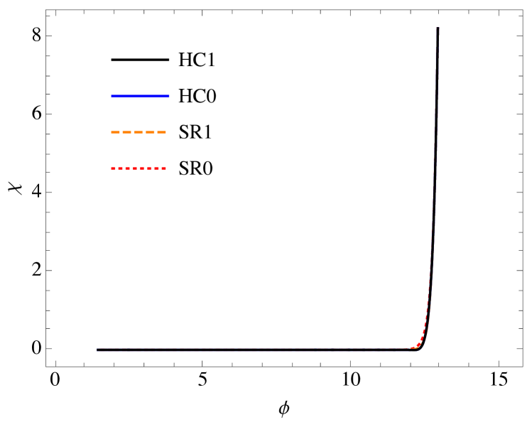
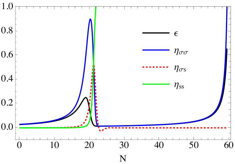
In Figure 1(b) we plot the evolution of the slow-roll parameters for the trajectory under consideration. Here $\epsilon$ is as defined in eq. (1.4), while $\eta_{\sigma\sigma}$, $\eta_{\sigma s}$ and $\eta_{ss}$ correspond to projections of $\eta_{IJ}$ – as defined in eq. (2.16) – on to the kinematic basis vectors $e^{I}_{\sigma}$ and $e^{I}_{s}$, which lie parallel and perpendicular to the background trajectory respectively. As an example, we have $\eta_{\sigma s}=e^{I}_{\sigma}\eta_{IJ}e^{J}_{s}$. It is helpful to use these projections of $\eta_{IJ}$ as at lowest order in slow-roll they are easy to interpret physically. In particular, one finds that $\eta\simeq-2\eta_{\sigma\sigma}+4\epsilon^{(0)}$ and $\theta^{\prime}\simeq-\eta_{\sigma s}$, where $\theta$ is the angle between the tangent of the trajectory and the $\phi$ axis [42]. As such, $\eta_{\sigma\sigma}$ is related to the rate at which $\epsilon$ evolves, while $\eta_{\sigma s}$ is related to the rate at which the trajectory turns. Whether or not the trajectory turns is important when considering the temporal evolution of $\zeta$. In the presence of so-called isocurvature perturbations, namely field fluctuations perpendicular to the background trajectory, it is known that the curvature perturbation $\zeta$ will be sourced by these isocurvature perturbations when the trajectory turns in field space. This means that non-zero values of $\eta_{\sigma s}$ will in general be associated with a non-conservation of $\zeta$ [42]. The final quantity $\eta_{ss}$ is related to the mass of the direction in field space that is perpendicular to the trajectory. If it is positive then we can expect neighbouring trajectories to converge, while if it is negative we can expect them to diverge. In this example we see that the quantities $\epsilon$, $\eta_{\sigma\sigma}$ and $\eta_{\sigma s}$ remain less than unity right up until the end of inflation. The oscillatory feature in $\eta_{\sigma s}$ at around $N\sim 20$ corresponds to the turning of the trajectory that we can see in Figure 1(a), and both $\epsilon$ and $\eta_{\sigma\sigma}$ become temporarily large around the time of the turn. We also see that, as the trajectory evolves into the minimum of the $\chi$-field potential, $\eta_{ss}$ evolves from being initially small to a positive value greater than unity. The fact that $\eta_{ss}$ becomes large and positive reflects the fact that the trajectory has reached an attractor where neighbouring trajectories converge. If the trajectory remains in the attractor for sufficiently long we expect a so-called adiabatic limit to be reached, in which the dynamics is effectively single-field in nature and so-called isocurvature perturbations perpendicular to the trajectory have decayed away. We expect $\zeta$ to be conserved in this limit.

(a)

(b)

(c)

(d)

Figure 2: (a) The evolution of $\mathcal{P}_{\zeta}/m^{2}$ for the same potential as considered in Figure 1. Results are shown for the four different slow-roll approximations SR0, SR1, HC0 and HC1, and for comparison we also show results calculated using the PyTransport code of Mulryne ’16 [40] (NUM). In (b) and (c) we show the evolution of $n_{s}$ and $N_{,A}N_{,A}$, respectively, as determined using the four different approximations SR0, SR1, HC0 and HC1. (d) The green dashed curve shows the ratio $(H^{(1)}/H^{(0)})^{2}$, where both quantities are evaluated at horizon crossing. The dashed orange and black curves correspond to the slow-roll corrections associated with slow-roll corrections to $\Sigma^{AB}$ in approximations SR1 and HC1, respectively.

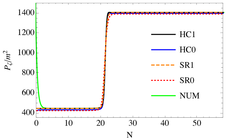
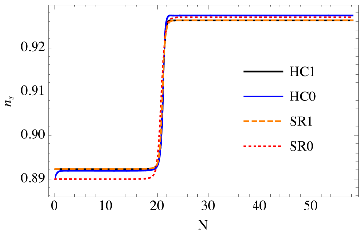
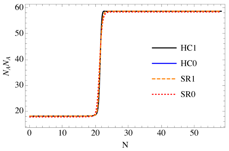
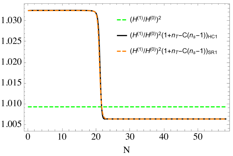
In Figure 2 we plot quantities relating to the two-point statistics of $\zeta$. The first panel shows the evolution of $\mathcal{P}_{\zeta}/m^{2}$ as determined using the five different levels of slow-roll approximation outlined at the beginning of this section. We see that both before and after the turn $\zeta$ is conserved, as expected. In the very early stages there appears to be a large discrepancy between the results of PyTransport, labeled NUM, and the other curves. However, this simply reflects the fact that decaying modes have been neglected in approximations SR0, SR1, HC0 and HC1, and we should therefore only expect them to coincide with the PyTransport result a few e-foldings after horizon crossing, which they do to very good approximation. At the end of inflation, all approximations are in agreement to within just over $1\%$. As we would naively expect, approximation SR0 deviates the most from the PyTransport result, while approximation $HC1$ provides the closest match. The second best approximation is SR1 rather than HC0, which suggests that the slow-roll corrections to $\Sigma^{AB}$ are important. Indeed, this is confirmed by the results plotted in Figures 2(c) & 2(d). In Figure 2(c) we have plotted the evolution of the quantity $N_{,A}N_{,A}$ for the four different approximations SR0, SR1, HC0 and HC1. This quantity determines how the perturbations in the initial conditions are related to $\delta N(=\zeta)$, and its evolution will depend on the approximations made in solving the super-horizon dynamics. Given that approximations HC0 and HC1 both use the full equations of motion to solve for the super-horizon evolution, we expect them to be in good agreement, which they are. Approximation SR1 is also in very good agreement with approximations HC0 and HC1, and even the leading-order approximation SR0 differs by less than $0.5\%$. In Figure 2(d) the corrections arising from slow-roll corrections to $\Sigma^{AB}$ are plotted for approximations SR1 and HC1. We see that these corrections are between $0.6$ and $0.7\%$. Finally, Figure 2(b) shows the evolution of $n_{s}$ as determined under the four different approximation schemes SR0, SR1, HC0 and HC1. The first thing to note is that the final value of $n_{s}$ is not in agreement with observations. The different approximations are in agreement at the $\sim 0.1\%$ level, with approximations SR1 and HC1 being in very close agreement. This again indicates that it is the slow-roll corrections to perturbations on the initial flat hypersurface that are dominant.

Overall, the very good agreement between the different approximations is perhaps surprising, considering that intermediately the slow-roll parameters become quite large. A similar behaviour was demonstrated for the non-Gaussianity parameter $f_{NL}$ in ref. [43], where they used a very different formalism. Presumably it is because the slow-roll parameters are only temporarily large that slow-roll corrections to observables do not become significant. It would be interesting to try and gain a more precise understanding as to how large slow-roll parameters must become and for how long in order for slow-roll corrections to become significant.

For the double quadratic model we find that $f_{NL}$ is unobservably small, so we do not consider its evolution in detail here.

5.2 Quadratic plus axion potential

Next we consider the axion-quadratic model that is also considered in [44, 16]. The potential takes the form

$$V=\frac{1}{2}m^{2}\phi^{2}+\Lambda^{4}\left(1-\cos\left(\frac{2\pi\chi}{f}\right)\right),$$ (5.2)

and we take

$$\Lambda^{4}=\frac{R^{2}m^{2}f^{2}}{4\pi^{2}}.$$ (5.3)

Doing so once again allows us to factor out the overall mass scale $m^{2}$, which is then only important when it comes to determining the overall magnitude of the power spectrum, i.e. $n_{s}-1$, $r$, $f_{NL}$ do not depend on $m$.

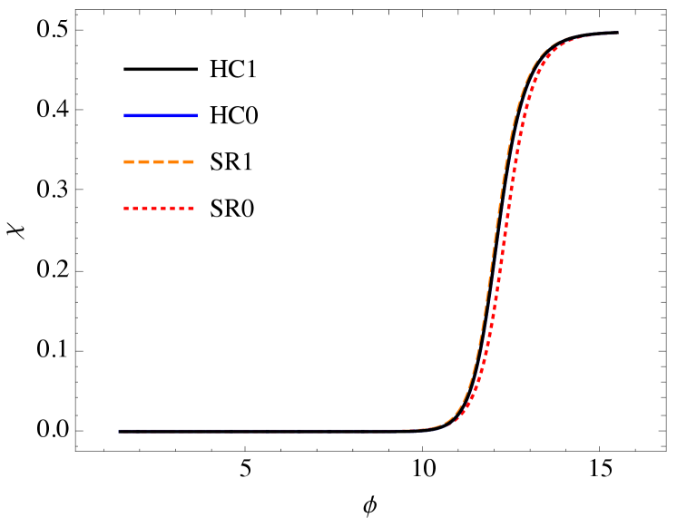
For the particular example considered here, we take $f=1$ and $R=5$. Seeing as we are interested in slow-roll corrections to $f_{NL}$, we choose initial conditions that are known to give rise to an observably large $f_{NL}$. Namely, $\chi$ is taken to start very close to the maximum of its potential. In using the PyTransport code we use the initial conditions $(\phi,\chi,\phi^{\prime},\chi^{\prime})=(16.4,(1-5\times 10^{-4})/2,0,0)$, and then consider the mode that leaves the horizon $8.2$ e-foldings after these initial conditions are set. When we calculate $f_{NL}$, the mode $k_{S}$ is again taken to leave at this time, and once again taking $R_{\rm sq}=0.1$ means that the mode $k_{L}$ left the horizon approximately $5.9$ e-foldings after the initial conditions were set. Solving the full background equations, we determine that after $8.2$ e-folds the field values are $(\phi_{k},\chi_{k})\simeq(15.42,0.4989)$, and we use these values as the initial conditions for calculating the results corresponding to approximations SR0, SR1, HC0 and HC1.

Plots of the background trajectory and the corresponding evolution of the slow-roll parameters are given in Figure 3, and we find that there are approximately $60$ e-foldings of inflation after horizon crossing. As can be seen from Figure 3(a), the trajectory evolves to the minimum of the $\chi$ potential before the end of inflation, and so we can expect that $\zeta$ becomes constant.

(a)

(b)

Figure 3: As in Figure 1 but for the quadratic plus axion potential outlined in the text, with $f=1$, $R=5$ and $(\phi_{k},\chi_{k})\simeq(15.42,0.4989)$.

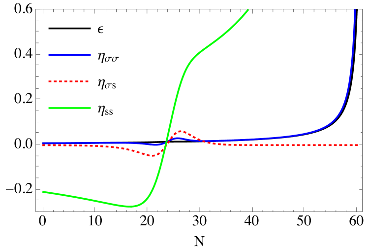
Looking at Figure 3(b), we see that in this example the quantities $\epsilon$, $\eta_{\sigma\sigma}$ and $\eta_{\sigma s}$ remain less than $0.1$ right up until the end of inflation. The oscillatory feature in $\eta_{\sigma s}$ at around $N\sim 25$ corresponds to the turning of the trajectory that we can see in Figure 3(a). The only relatively large slow-roll parameter, then, is $\eta_{ss}$. Initially it is negative, corresponding to when the trajectory is along the peak of the tachyonic $\chi$-field potential. At around $N\sim 25$ the trajectory then falls off the ridge and into the minimum of the $\chi$-field potential, where $\eta_{ss}$ is positive and neighbouring trajectories converge. The fact that $\eta_{ss}$ becomes large and positive reflects the fact that the trajectory has reached an attractor. As was mentioned before, if the trajectory remains in the attractor for sufficiently long we expect a so-called adiabatic limit to be reached.

(a)

(b)

(c)

(d)

Figure 4: As in Figure 2 but for the same quadratic plus axion potential as considered in Figure 3.

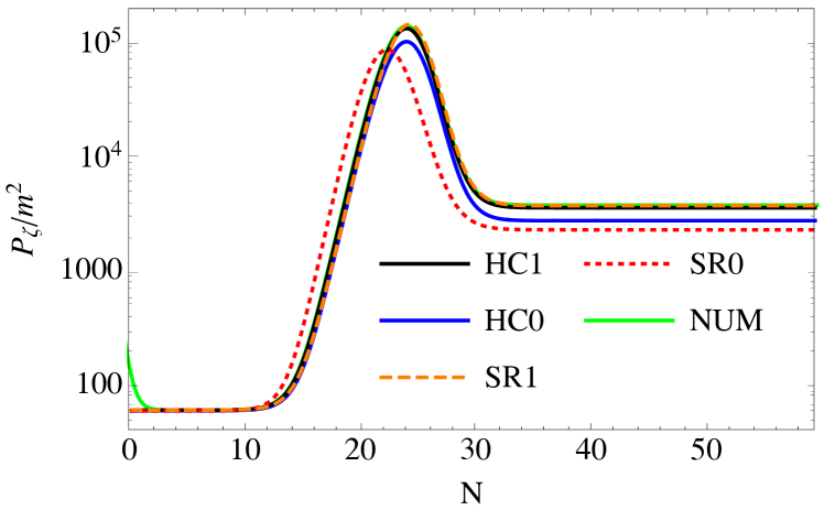
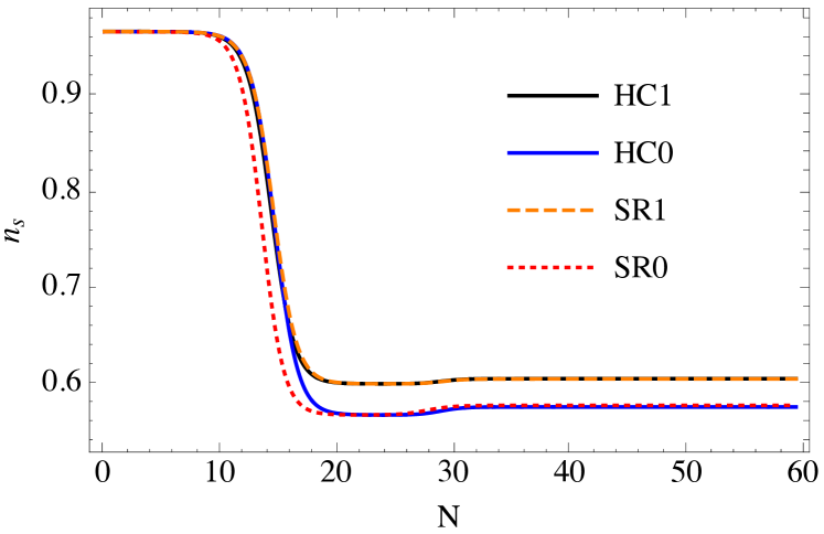
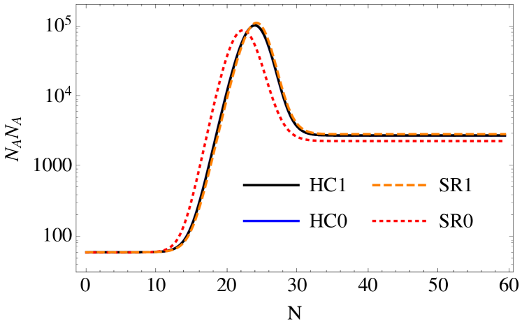
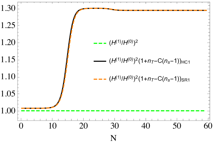
In Figure 4 we plot quantities relating to the two-point statistics of $\zeta$. The first panel shows the evolution of $\mathcal{P}_{\zeta}/m^{2}$ as determined using the five different levels of slow-roll approximation outlined at the beginning of this section. In the very early stages we see a large discrepancy between the NUM and other curves. However, as in the case of the double quadratic potential, this simply reflects the fact that decaying modes have been neglected in approximations SR0, SR1, HC0 and HC1, and we should therefore only expect them to coincide with the NUM curve a few e-foldings after horizon crossing. At later times, we see that approximations HC1 and SR1 are in very good agreement with the PyTransport results NUM. For the first 10-efoldings the trajectory remains straight and $\zeta$ is conserved. The trajectory then starts to bend, leading to a sourcing of $\zeta$, but after $N\sim 30$ the trajectory reaches the minimum of the $\chi$ potential and $\zeta$ is once again conserved. Although qualitatively all five curves are in good agreement, quantitatively we find a discrepancy of over $60\%$ in the final value of $\mathcal{P}_{\zeta}$. As approximations HC0 and HC1 essentially only differ in their assumptions for the power spectra of the initial field fluctuations, i.e. $\Sigma^{AB}$, Figure 4(a) suggests that slow-roll corrections arising from the slow-roll corrections to $\Sigma^{AB}$ must be important. Indeed, in Figure 4(d) we plot the corrections due to slow-roll corrections to $\Sigma^{AB}$, and one can see that they are on the order of $\sim 30\%$. In Figure 4(c) we plot the evolution of the quantity $N_{,A}N_{,A}$ for the four different approximations SR0, SR1, HC0 and HC1. Given that approximations HC0 and HC1 both use the full equations of motion to solve for the super-horizon evolution, we see that they are in perfect agreement. We also see that the next-to-leading order approximation used in SR1 gives a significant improvement over the leading-order approximation SR0. The discrepancy between SR0 and HC1 is on the order $20\%$. Finally, Figure 4(b) shows the evolution of $n_{s}$ as determined under the four different approximation schemes. The first thing to note is that the final value of $n_{s}$ is not in agreement with observations. As discussed in Section 4.2.1, a consequence of this will be that slow-roll corrections from the initial conditions are large, which we indeed see to be the case in Figure 4(d). This is further reflected in the large discrepancy between the HC0 and HC1 curves in Figure 4(b), as essentially the only difference between these approximation schemes is the choice of the initial $\Sigma^{AB}$.

(a)

(b)

(c)

Figure 5: Quantities relating to $f_{NL}$ for the quadratic plus axion potential considered in Figures 3 & 4: (a) Evolution of $f_{NL}$ as determined using the four approximations SR0, SR1, HC0 and HC1, with numerical results calculated using the code PyTransport [40] also given for comparison (NUM). (b) Evolution of $\tilde{f}_{NL}$ as determined using the four approximations SR0, SR1, HC0 and HC1. (c) Evolution of the slow-roll corrections associated with slow-roll corrections to the initial $\Sigma^{AB}$ for the approximations SR1 and HC1.

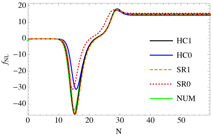
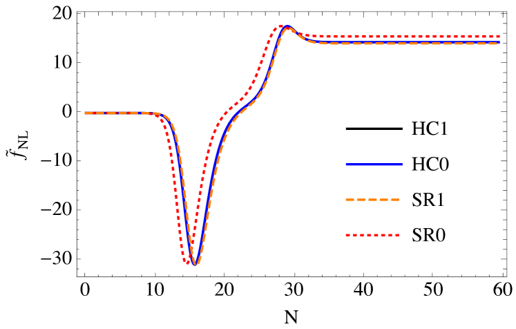
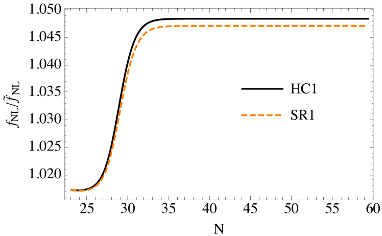
In Figure 5 we plot quantities related to $f_{NL}$. Looking at Figure 5(a) we see that discrepancies between the various approximation schemes can be large intermediately. In particular, the magnitudes of the minima at around $N\sim 15$ differ by around $50\%$. Interestingly, the magnitudes of the minima as determined using approximations SR0 and HC0 are very similar, as are those determined using approximations SR1 and HC1. This suggests that at this intermediate time it is the slow-roll corrections to $\Sigma^{AB}$ that are important. This is also reflected in Figure 5(b), where $f_{NL}$ neglecting slow-roll corrections to $\Sigma^{AB}$, namely $\tilde{f}_{NL}$, is plotted for the four different approximation schemes. In this plot we see that the magnitudes of the minima at around $N\sim 15$ are very similar for all the approximation schemes, while the location of the minimum is around two e-foldings earlier for approximation SR0. Turning to the final value of $f_{NL}$, we find that the different approximations are in better agreement, with differences being less than $10\%$. From Figure 5(b) we see that $\tilde{f}_{NL}$ as determined by HC1, HC0 and SR1 are approximately $10\%$ lower than the SR0 result. In Figure 5(c) we plot the slow-roll corrections arising from slow-roll corrections to $\Sigma^{AB}$, namely $f_{NL}/\tilde{f}_{NL}$, and for the cases HC1 and SR1 we see that they give a positive correction of just under $5\%$.

In summary, compared to the double quadratic model considered in the preceding subsection, we have found slow-roll corrections to be much larger in this model with a quadratic plus axion potential. This is perhaps to be expected given that the slow-roll parameter $\eta_{ss}$ in this model is relatively large and negative for an extended period, namely the first $\sim 20$ e-foldings after horizon exit. Interestingly, we found that corrections to the non-Gaussianity parameter $f_{NL}$ were significantly smaller than those to the power spectrum.

5.3 Linear plus axion potential

Next we consider a very similar model to that considered above, but replace the quadratic potential of the $\phi$-field with a linear potential. It has been shown in [45, 46] that such a linear potential may be realised from axion monodromy. As we will see, with this potential we are able to find a region in parameter space for which the predictions for $n_{s}$ are in agreement with observations. The potential thus takes the form

$$V=\lambda\phi+\Lambda^{4}\left(1-\cos\left(\frac{2\pi\chi}{f}\right)\right),$$ (5.4)

and similar to the previous case we take

$$\Lambda^{4}=\frac{\lambda f^{2}}{\mathcal{M}4\pi^{2}}.$$ (5.5)

$\lambda$ can then be factored out and it only affects the overall normalisation of $\mathcal{P}_{\zeta}$, with $\mathcal{P}_{\zeta}\propto H_{k}^{2}=V_{k}/(3-\epsilon_{k})\propto\lambda$.

We take $f=1/10$ and $\mathcal{M}=1$, and as in the previous case we choose initial conditions such that an observably large $f_{NL}$ is generated. In using the PyTransport code we set initial conditions as $(\phi,\chi,\phi^{\prime},\chi^{\prime})=(11.6,(1-1.5\times 10^{-3})/20,0,0)$, and consider a mode that leaves the horizon 8.2 e-foldings after these initial conditions are set. In calculations of $f_{NL}$ we once again take $k_{S}$ to leave the horizon at this time, and we choose $R_{\rm sq}=0.1$ such that $k_{L}$ left the horizon approximately $5.9$ e-foldings after the initial conditions were set. Using the full equations of motion we find that after 8.2 e-folds the field values are given as $(\phi_{k},\chi_{k})\simeq(10.90,0.04985)$, and these are the values used as initial conditions in approximations SR0, SR1, HC0 and HC1. After horizon crossing we find that there are approximately $60$ e-foldings of inflation.

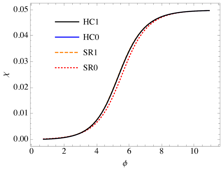
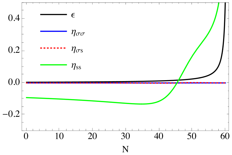
In Figure 6(a) we give the background trajectory as calculated using the different approximations SR0, SR1, HC0 and HC1. As in the previous example, the initial trajectory is along the maximum of the $\chi$-field potential, but eventually it falls into the minimum at $\chi=0$ and continues to evolve in the $\phi$ direction. Compared to the trajectory shown in Figure 3(a) we see that the transition into the minimum of the $\chi$ potential is much more gradual, but nevertheless the trajectory does reach the minimum before the end of inflation. We can thus expect that $\zeta$ will approach a constant towards the end of inflation.

In Figure 6(b) we plot the evolution of the slow-roll parameters described in the previous subsection. We see that $\eta_{\sigma\sigma}$ and $\eta_{\sigma s}$ remain very small for the entire duration of inflation. The fact that $\eta_{\sigma s}$ remains much smaller in this example than in the previous example reflects the fact that the turning of the trajectory in the transition to the minimum of the $\chi$ potential is much more gradual. Qualitatively we see that the evolution of $\eta_{ss}$ is similar to that in the previous example. Quantitatively, however, the initial tachyonic mass in the $\chi$ direction is smaller in this case, and we also see that the transition to positive $\eta_{ss}$ – which indicates the time at which the transition to the minimum of the $\chi$ potential occurs – occurs much later on in this example, at around $N\sim 45$. This again is consistent with our observation that evolution in the $\chi$ direction occurs on a longer timescale in this example.

(a)

(b)

Figure 6: As in Figure 1 but for the linear plus axion potential outlined in the text, with $f=1/10$, $\mathcal{M}=1$ and $(\phi_{k},\chi_{k})\simeq(10.90,0.04985)$.

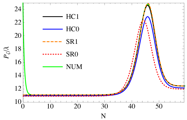
In Figure 7(a) we plot the evolution of $\mathcal{P}_{\zeta}/\lambda$ as determined using the approximations SR0, SR1, HC0 and HC1, with numerical results calculated using the PyTransport code [40] also given for comparison. In the early stages we see that it takes approximately four e-foldings before the decaying modes become negligible and the approximations SR0, SR1, HC0 and HC1 come into good agreement with the NUM curve. Throughout the remaining evolution we find that the SR1 and HC1 approximations are in very good agreement with the results obtained using PyTransport. As expected after looking at the background trajectory in Figure 6, we see that the curvature perturbation approaches a constant right at the end of inflation, which is much later on than in the previous example. Qualitatively the SR0 approximation is in good agreement with the PyTransport results NUM and the other approximations. Quantitatively, however, we see that the peak in $\mathcal{P}_{\zeta}/\lambda$ is about $10\%$ lower than the NUM curve and also occurs about two e-foldings earlier. Looking at the final value of $\mathcal{P}_{\zeta}/\lambda$, we see that corrections to approximation SR0 are less than $5\%$. The discrepancy between approximations HC0 and HC1 highlights the importance of slow-roll corrections to the initial power spectra $\Sigma^{AB}$, as this is essentially the only difference between these two approximations. We also note that, as in the previous example, the next-to-leading order approximation SR1 offers a significant improvement over the lowest order approximation SR0.

(a)

(b)

(c)

(d)

Figure 7: Essentially as in Figure 2 but for the linear plus axion potential considered in Figure 6. The only difference is that the normalised power spectrum is given as $\mathcal{P}_{\zeta}/\lambda$ as opposed to $\mathcal{P}_{\zeta}/m^{2}$.

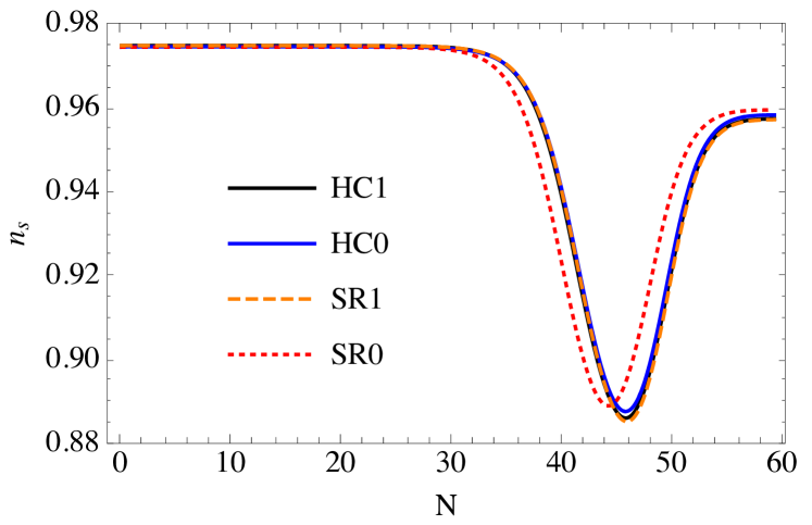
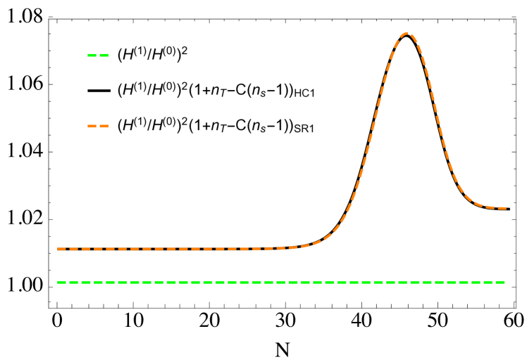
In Figure 7(b) we show the evolution of $n_{s}$ as determined using the four approximations SR0, SR1, HC0 and HC1. Looking at the final values we see that they are in very good agreement, with corrections to the SR0 approximation being less than half of a percent. Another important thing to note is that the final value of $n_{s}$ is consistent with current observations. This is consistent with the fact that slow-roll corrections to $\mathcal{P}_{\zeta}$ are relatively small. As we saw in Section 4.2.1, slow-roll corrections to $\mathcal{P}_{\zeta}$ arising from slow-roll corrections to $\Sigma^{AB}$ can be written in terms of $n_{s}-1$, and if $n_{s}-1$ is in agreement with observations then this implies that the slow-roll corrections associated with corrections to $\Sigma^{AB}$ should be small. Indeed, this is confirmed explicitly in Figure 7(d), where the slow-roll corrections associated with corrections to the initial power spectra $\Sigma^{AB}$ are plotted as a function of time for the approximations SR1 (orange dashed curve) and HC1 (solid black curve). We see that at the end of inflation these corrections are just over $2\%$. For reference, the green dotted curve also shows the ratio $(H^{(1)}/H^{(0)})^{2}$, with both quantities evaluated at horizon crossing. Given that this ratio is so close to unity, we see that slow-roll corrections associated with $\Sigma^{AB}$ mostly come from the factor $(1+n_{T}-Cn_{\zeta})$.

Given that slow-roll corrections arising from corrections to the initial power spectra $\Sigma^{AB}$ are small, the only way to obtain large corrections to $\mathcal{P}_{\zeta}$ would be if slow-roll corrections to the super-horizon dynamics were large. Such corrections are encoded in the quantity $N_{,A}N_{,A}$, which is plotted for the four different approximations in Figure 7(c), and we see that corrections to the SR0 approximation are less than $2\%$ at the end of inflation. Also note that the HC0 and HC1 curves are in very good agreement, which is to be expected given that they both use the full equations of motion to solve for the super-horizon evolution. The approximation SR1 also offers a significant improvement over the SR0 approximation, being in very good agreement with approximations HC0 and HC1.

(a)

(b)

(c)

Figure 8: As in Figure 5 but for the linear plus axion potential considered in Figures 6 & 7.

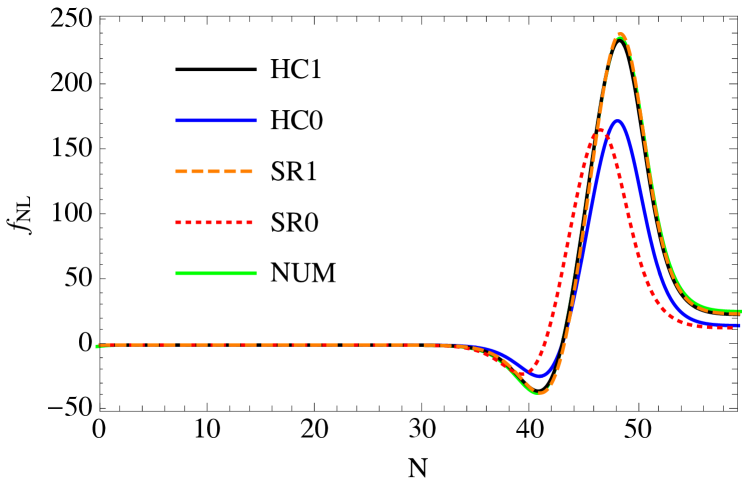
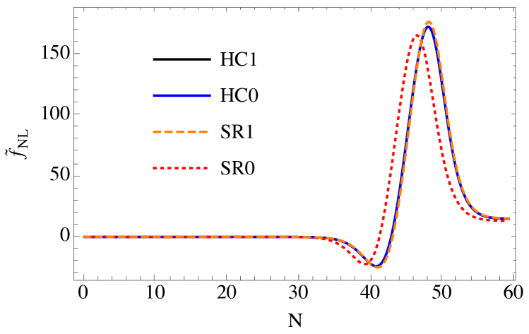
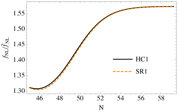
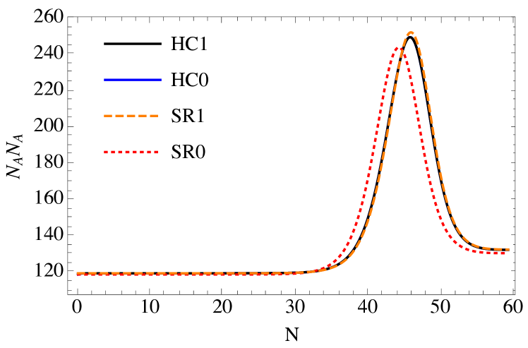
Turning next to the non-Gaussianity, we plot quantities relating to $f_{NL}$ in Figure 8. As with the previous example, we see that intermediately the peak values of $f_{NL}$ are quite different for the different approximations, with approximations SR1 and HC1 giving peak values $\sim 40$% larger than approximations SR0 and HC0. The discrepancy between the peak values given by HC0 and HC1 suggests that the difference can be attributed to the slow-roll corrections arising from slow-roll corrections to $\Sigma^{AB}$, and this is confirmed in Figure 8(b), where we see that $\tilde{f}_{NL}$ essentially coincides for approximations HC0 and HC1. As with the power spectrum, we also find that the peak in $f_{NL}$ as determined using approximation SR0 occurs a couple of e-foldings earlier than for the other approximations. Focussing next on the final value of $f_{NL}$, we find that corrections to the SR0 approximation are very large. The approximation HC1 gives a value almost $80$% larger than the SR0 result, and the PyTransport result NUM is then almost $10$% larger than approximation HC1. Corrections to the SR0 result for $\tilde{f}_{NL}$ are less than $15$%, so it is the slow-roll corrections from $\Sigma^{AB}$ that are mostly responsible for the large discrepancies. This is confirmed in Figure 8(c), where we plot $f_{NL}/\tilde{f}_{NL}$ and see that corrections from the factor $1-n_{T}^{(0)}-\tilde{n}_{\delta b}[2C-\ln(R_{\rm sq})]$ appearing in eq. (4.37) are close to $60$%. Given that $n_{T}^{(0)}$ is small, this suggests that $n_{\delta b}$ is relatively large in this model.

(a)

(b)

(c)

Figure 9: Predictions for the linear plus axion potential with $\mathcal{M}=25/49$. The decay constant is varied over the range $-2\leq\log_{10}(f)\leq 1$ and the initial value of $\chi$ is varied over the range $0\leq-\log_{10}(1-2\chi_{k}/f)\leq 3$. The initial value of $\phi$ is determined by requiring a total of $60$ e-foldings of inflation, with the end of inflation being defined as when $\epsilon^{(0)}=1$. Approximation HC1 is used. (a) Predictions for $n_{s}$. The solid black line corresponds to the central observed value and the dashed line is the $2\sigma$ lower bound. (b) Predictions for $r$. (c) Predictions for $f_{NL}$. The dashed and solid black lines correspond to the $1$- and $2$-$\sigma$ upper bounds respectively. The white region corresponds to where $f_{NL}>50$.

In summary, as in the previous example, we have found that slow-roll corrections in this model with a linear plus axion potential can be significant. This is not surprising given that the slow-roll parameter $\eta_{ss}$ is relatively large and negative for an extended period of $\sim 40$ e-foldings after horizon exit. Interestingly, unlike the previous example, we have found that it is the slow-roll corrections to $f_{NL}$ that are most significant, with slow-roll corrections to the power spectrum being relatively small.

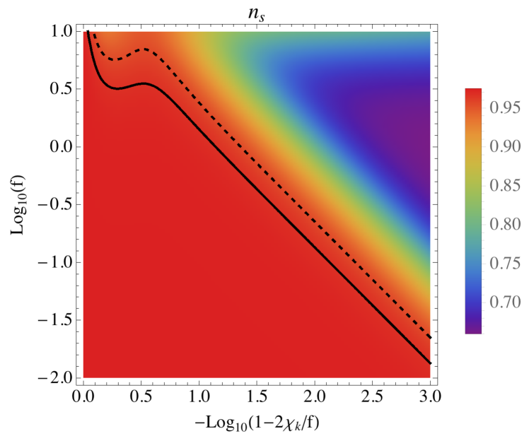
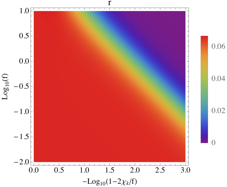
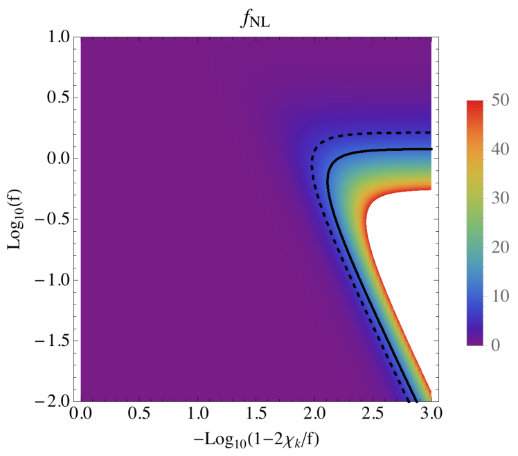
Given that predictions for $n_{s}-1$ appear to be in agreement with observations in this model, it is perhaps interesting to take a closer look at how the predictions depend on the model parameters. In Figure 9, taking $\mathcal{M}=25/49$ we plot the predictions for $n_{s}$, $r$ and $f_{NL}$ as a function of the value of $\chi$ at horizon crossing, $\chi_{k}$, and $f$. All predictions are calculated using approximation HC1. We parametrise $\chi_{k}$ in terms of how far it deviates from the maximum of the $\chi$-field potential as $\chi_{k}=(f/2)(1-10^{-x})$. We then vary $x$ from $0$ to $3$. For $f$ we take values in the range $10^{-2}\leq f\leq 10$. In each case, the initial value of $\phi$ is determined by requiring that $60$ e-foldings of inflation are obtained, with the condition for the end of inflation being $\epsilon^{(0)}=1$. This range of parameters has been chosen such that inflation is essentially driven by the $\phi$ potential and so that all trajectories converge to the minimum of the $\chi$ potential before the end of inflation, in order that the final value of $\zeta$ approaches a constant. In Figure 9(a) the solid black line represents the central observed value $n_{s}=0.968$, with the dashed line being the lower $2\sigma$ bound [1]. As such, we see that just under half of the parameter space considered is ruled out by observations. In Figure 9(b) we plot the predictions for $r$. At $2\sigma$ $r=0$ is still not ruled out, and the constraint $r<0.1$ does not rule out any of the parameter space considered here. Finally, in Figure 9(c) we plot the predictions for $f_{NL}$. Here we can clearly see that observably large $f_{NL}$ is only obtained when $\chi$ is tuned to start very close to the top of its potential. The black solid line corresponds to the $2\sigma$ upper bound of $f_{NL}=10.8$ while the dashed line is the $1\sigma$ upper bound of $f_{NL}=5.8$ [2].

Figure 10: Combined $1$- and $2$-$\sigma$ constraints in the $\chi_{k}$–$f$ plane for the linear plus axion model with $\mathcal{M}=25/49$. Solid shaded regions correspond to excluded regions as determined using approximation HC1, while the dashed lines indicate how the excluded regions change if one uses approximation SR0.

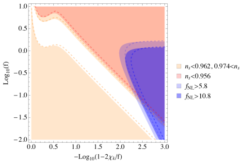
In Figure 10 we combine the constraints coming from $n_{s}$, $r$ and $f_{NL}$. The light- and dark-blue regions are the $1$- and $2$-$\sigma$ excluded regions associated with constraints on $f_{NL}$. The orange and red shaded regions are the $1$- and $2$-$\sigma$ excluded regions associated with constraints on $n_{s}$. $2\sigma$ constraints on $r$ do not rule out any of the parameter space. The dashed curves with matching colours indicate how the excluded regions change if approximation SR0 is used instead of HC1 to determine the predictions. If we focus on the $2\sigma$ constraints on $n_{s}$ and $f_{NL}$, we see that the allowed region is larger if we use approximation SR0.

Figure 11: Predictions in the $n_{s}$–$f_{NL}$ plane for the linear plus axion model with $\mathcal{M}=25/49$. The different coloured lines correspond to different choices of $f$, as given in the plot legend. Solid lines are the predictions as determined using approximation HC1, while dashed lines are those determined using approximation SR0. In all cases, the ends of the curves located to the bottom right-hand side of the figure correspond to $\chi_{k}=0$, where predictions coincide with linear chaotic inflation. The initial value of $\chi$ then increases as we move left and upwards along the curves. The blue shaded regions correspond to the $1$- and $2$-$\sigma$ constraints on $n_{s}$, while the orange shaded regions correspond to the $1$- and $2$-$\sigma$ constraints on $f_{NL}$.

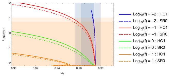
In Figure 11 we plot the predictions for $f_{NL}$ as a function of the predictions for $n_{s}$, taking $\log_{10}(f)=-2,-1,0,1$. The solid and dashed lines correspond predictions as calculated using approximations HC1 and SR0, respectively. Different points along any given line correspond to different initial conditions for $\chi$. For $\chi_{k}=0$ the predictions for any $f$ coincide with those of linear chaotic inflation, and this is the point at which the lines converge in the bottom right-hand corner of the plot. Moving left and upwards along any given line then corresponds to increasing the initial value of $\chi$. In the case of $\log_{10}(f)=-2$ we can see the other end of the line, which corresponds to $-\log_{10}(1-2\chi_{k}/f)=3$. For observationally relevant values of $n_{s}$ we see that only the curves corresponding to $\log_{10}(f)=-2$ and $\log_{10}(f)=-1$ predict observable values of $f_{NL}$, and these values do differ depending on whether approximation SR0 or HC1 is used.

6 Summary and Conclusions

Motivated by the need for high-precision theoretical predictions to compare with current and future data, in this paper we have investigated the importance of slow-roll corrections in determining predictions for the curvature perturbation $\zeta$ in multi-field models of inflation. In our analysis we made use of the separate universes approach and $\delta N$ formalism, which allowed us to consider slow-roll corrections to the non-Gaussianity of $\zeta$ as well as corrections to its two-point statistics. In the context of the $\delta N$ formalism, slow-roll corrections to the correlation functions of $\zeta$ can essentially be divided into two categories. First one has corrections associated with slow-roll corrections to the correlation functions $\Sigma^{AB}$ of the field perturbations on the initial flat hypersurface at horizon crossing. Second one has slow-roll corrections to the derivatives of $N$ with respect to the field values on the initial flat slice, $N_{,A}$ and $N_{,AB}$.

Slow-roll corrections to the correlation functions of the field perturbations on the initial flat hypersuface can be calculated by solving the perturbation equations of motion around the horizon-crossing time, and we have made use of the next-to-leading order results derived by Nakamura & Stewart [30]. We find that the corrections to $\zeta$ arising from these slow-roll corrections can be written in a compact form, with expressions for $\mathcal{P}_{\zeta}$, $n_{s}$, $r$ and $f_{NL}$ being given in eqs. (4.17), (4.20), (4.28) and (4.37) respectively. The expressions for corrections to $\mathcal{P}_{\zeta}$, $r$ and $n_{s}$ are in agreement with those derived using different methods in [37, 9]. To our knowledge, the compact expression for corrections to $f_{NL}$ has not previously been given explicitly in the literature. An appealing feature of the compact expressions is that the slow-roll corrections associated with $\Sigma^{AB}$ are written in terms of quantities that in principle are observable. In particular, slow-roll corrections to $\mathcal{P}_{\zeta}$ and $r$ contain terms proportional to $n_{s}-1$ and $n_{T}$. The fact that $n_{s}-1$ is now tightly constrained by observations, and that barring an exact cancellation amongst terms we have $|n_{T}|\lesssim|n_{s}-1|$, means that slow-roll corrections to $\mathcal{P}_{\zeta}$ and $r$ for any observationally viable model are constrained to be small. Similarly, slow-roll corrections to $n_{s}$ and $f_{NL}$ include terms proportional to $\alpha_{s}$ and $n_{\delta b}$ respectively. Observational constraints on $\alpha_{s}$ imply that for observationally viable models these slow-roll corrections to $n_{s}$ are relatively small. We are unaware, however, of any similar constraints on $n_{\delta b}$ at the present time, meaning that these slow-roll corrections to $f_{NL}$ are not necessarily constrained to be small, even for observationally viable models.

Slow-roll corrections to the quantities $N_{,A}$ and $N_{,AB}$ arise from using different levels of slow-roll approximation in solving for the super-horizon evolution, which in turn corresponds to using different levels of slow-roll approximation in the background equations of motion. We have considered four different levels of approximation, which we labelled SR0, SR1, HC0 and HC1. SR0 corresponds to assuming that the lowest order slow-roll equations of motion – given in eq. (2.12) – hold throughout the super-horizon evolution. Similarly, SR1 corresponds to assuming that the next-to-leading order slow-roll equations of motion – given in eq. (2.18) – hold throughout inflation. Approximations HC0 and HC1, on the other hand, use the full equations of motion on super-horizon scales, only assuming that slow-roll is a good approximation around horizon crossing. The fact that slow-roll is assumed to hold around horizon crossing means that only initial field values need to be specified, with the initial field velocities being given by the leading and next-to-leading order relations (2.12) and (2.18) for HC0 and HC1 respectively. Note that we were forced to assume that the slow-roll approximation holds around the horizon crossing time due to the fact that we made use of the results of Nakamura & Stewart for $\Sigma^{AB}$. Although we expect approximations HC0 and HC1 to more correctly reproduce the super-horizon evolution, the advantage of approximations SR0 and SR1 is that fewer equations have to be solved. If we wish to expand $\delta N$ up to second order in the initial field perturbations we find that for approximations HC0 and HC1 the number of equations we must solve goes as $M^{3}$ for large $M$, where $M$ is the number of fields. For approximations SR0 and SR1, however, the number is half that, going as $M^{3}/2$. As such, if we are considering models with many fields, SR0 and SR1 will be numerically advantageous provided they give sufficiently accurate results.

To our knowledge, the next-to-leading order slow-roll equations of motion used in approximation SR1 have not received much attention in the literature up to now. For the examples considered in Section. 5, however, we found that approximation SR1 offers a significant improvement over SR0, often being in very good agreement with approximation HC1 and the results obtained using PyTransport [40]. In two of the examples considered, we found that corrections to the leading order approximation SR0 could be sizeable, on the order of tens of percent. The quadratic plus axion model gave an example where predictions for $n_{s}-1$ deviated significantly from the observed value, which in turn meant that corrections to $\mathcal{P}_{\zeta}$ coming from slow-roll corrections to $\Sigma^{AB}$ were large. Corrections to $f_{NL}$ in this model, however, were relatively small, being less than $10\%$. The linear plus axion model offered a good example where corrections to the power spectrum were relatively small, at less than $5\%$, but corrections to the non-Gaussianity were large, being around $95\%$. In this case, even corrections to the approximation HC1 as compared to the results obtained using PyTransport were found to be on the order of $10\%$, which suggests that it may be necessary to go to next-to-next-to-leading order in the slow-roll expansion at horizon crossing to obtain predictions of the desired precision.

Finally, in the model with a double quadratic potential we found that all slow-roll corrections remained small. This was perhaps somewhat surprising given that intermediately some of the slow-roll parameters became quite large. We take this to indicate that the slow-roll parameters were not large enough for long enough to give rise to significant corrections. Indeed, in the other two models considered one of the slow-roll parameters was relatively large for an extended period after the horizon crossing time.

In terms of future directions, it would be desirable to determine compact expressions for slow-roll corrections to the quantities $N_{,A}$ and $N_{,AB}$, in order that the conditions under which they become large could be better understood. This would help us to better understand why slow-roll corrections remained small in the model with a double quadratic potential, despite the slow-roll parameters intermediately becoming large. Also, for models that give rise to slow-roll corrections on the order of tens of percent, it will likely be necessary to consider next-to-next-to-leading order corrections in order to obtain predictions of the desired precision. The correlation functions of the initial field perturbations up to this order in slow-roll have been determined using a Green’s function method in [32], so these results could be used. It would then be necessary to determine the background field equations at next-to-next-to-leading order in slow roll. Finally, when using the lowest-order background equations of motion it is known that for some classes of potentials the derivatives of $N$ can be determined analytically. It would be interesting to explore whether analytical results can also be obtained when using the next-to-leading order background equations.

Appendix A Background equations of motion at next-to-leading order in slow-roll

In order to expand the equations of motion in eq. (2.6) up to higher orders in the slow-roll approximation we first write them as

$$\phi_{I}^{\prime}=U_{,I}-\frac{\xi\phi_{I}^{\prime\prime}}{3-\frac{\xi}{2}\phi_{I}^{\prime}\phi_{I}^{\prime}},$$ (A.1)

where $U$ is defined as

$$U\equiv-\ln V$$ (A.2)

In the above expression we also used eq. (2.8) and introduced a parameter $\xi$ (not to be confused with the parameter $\xi=1/(LH)$ used in Section 3) to help us organise small terms in the computations that follow. Initially we take $\xi\ll 1$ and expand eq. (A.1) and fields $\phi_{I}$ in terms of $\xi$. The latter expansion can be written as

$$\phi_{I}=\phi_{I}^{\textsc{{\tiny$\left(0\right)$}}}+\xi\phi_{I}^{\left(1\right)}+\mathcal{O}\left(\xi^{2}\right).$$ (A.3)

At the end of the computations we take $\xi=1$.

Plugging eq. (A.3) into eq. (A.1) and expanding in terms of $\xi$ we find

$${\phi_{I}^{\textsc{{\tiny$\left(0\right)$}}}}^{\prime}+\xi{\phi_{I}^{\textsc{{\tiny$\left(1\right)$}}}}^{\prime}+\mathcal{O}\left(\xi^{2}\right)=U_{,I}^{\textsc{{\tiny$\left(0\right)$}}}+\xi\left(U_{,IJ}^{\textsc{{\tiny$\left(0\right)$}}}\phi_{J}^{\textsc{{\tiny$\left(1\right)$}}}-\frac{1}{3}{\phi_{I}^{\textsc{{\tiny$\left(0\right)$}}}}^{\prime\prime}\right)+\mathcal{O}\left(\xi^{2}\right),$$ (A.4)

where $U_{,I}^{\textsc{{\tiny$\left(0\right)$}}}$ and $U_{,IJ}^{\textsc{{\tiny$\left(0\right)$}}}$ are functions of fields $\phi_{I}^{\textsc{{\tiny$\left(0\right)$}}}$, for example

$$U_{,I}^{\textsc{{\tiny$\left(0\right)$}}}\equiv\frac{\partial U\left(\vec{\phi}^{\textsc{{\tiny$\left(0\right)$}}}\right)}{\partial\phi_{I}^{\textsc{{\tiny$\left(0\right)$}}}}$$ (A.5)

and similarly

$$U_{,IJ}^{\textsc{{\tiny$\left(0\right)$}}}\equiv\frac{\partial^{2}U\left(\vec{\phi}^{\textsc{{\tiny$\left(0\right)$}}}\right)}{\partial\phi_{I}^{\textsc{{\tiny$\left(0\right)$}}}\partial\phi_{J}^{\textsc{{\tiny$\left(0\right)$}}}}.$$ (A.6)

At the zeroth order in $\xi$ eq. (A.4) becomes

$${\phi_{I}^{\textsc{{\tiny$\left(0\right)$}}}}^{\prime}\simeq U_{,I}^{\textsc{{\tiny$\left(0\right)$}}}.$$ (A.7)

Taking the time derivative of this expression and plugging back into eq. (A.4) we get

$${\phi_{I}^{\textsc{{\tiny$\left(0\right)$}}}}^{\prime}+\xi{\phi_{I}^{\textsc{{\tiny$\left(1\right)$}}}}^{\prime}\simeq U_{,I}^{\textsc{{\tiny$\left(0\right)$}}}+\xi\left[U_{,IJ}^{\textsc{{\tiny$\left(0\right)$}}}\phi_{J}^{\textsc{{\tiny$\left(1\right)$}}}-\frac{1}{3}U_{,IJ}^{\textsc{{\tiny$\left(0\right)$}}}U_{,J}^{\textsc{{\tiny$\left(0\right)$}}}\right],$$ (A.8)

where we kept only terms up to the first order in $\xi$.

In the last expression derivatives of $U^{\textsc{{\tiny$\left(0\right)$}}}$ are functions of the fields $\phi_{I}^{\textsc{{\tiny$\left(0\right)$}}}$, but for our purpose the above equation is more useful if expressed as a closed system of equations for the fields

$$\phi_{1I}\equiv\phi_{I}^{\textsc{{\tiny$\left(0\right)$}}}+\xi\phi_{I}^{\textsc{{\tiny$\left(1\right)$}}}.$$ (A.9)

To do that, we can compute

$$U_{,I}\left(\vec{\phi}_{1}\right)=U_{,I}^{\textsc{{\tiny$\left(0\right)$}}}+\xi U_{,IJ}^{\textsc{{\tiny$\left(0\right)$}}}\phi_{J}^{\textsc{{\tiny$\left(1\right)$}}}+\mathcal{O}\left(\xi^{2}\right),$$ (A.10)

where we defined

$$U_{,I}\left(\vec{\phi}_{1}\right)\equiv\frac{\partial U\left(\vec{\phi}_{1}\right)}{\partial\phi_{1I}}.$$ (A.11)

Similarly the second derivative of $U$ for fields $\phi_{1I}$ can be easily obtained

$$U_{,IJ}\left(\vec{\phi}_{1}\right)=U_{,IJ}^{\textsc{{\tiny$\left(0\right)$}}}+\xi U_{,IJK}^{\textsc{{\tiny$\left(0\right)$}}}\phi_{K}^{\textsc{{\tiny$\left(1\right)$}}}+\mathcal{O}\left(\xi^{2}\right),$$ (A.12)

where the definition of $U_{,IJ}\left(\vec{\phi}_{1}\right)$ is analogous to the one of $U_{,I}\left(\vec{\phi}_{1}\right)$ in eq. (A.11).

Finding next the expression for $\xi U_{,IJ}^{\textsc{{\tiny$\left(0\right)$}}}\phi_{J}^{\textsc{{\tiny$\left(1\right)$}}}$from eq. (A.10) and $U_{,IJ}^{\textsc{{\tiny$\left(0\right)$}}}$ from eq. (A.12) and plugging the result into eq. (A.8) we compute

$$\phi_{1I}^{\prime}\simeq U_{,I}\left(\vec{\phi}_{1}\right)-\frac{\xi}{3}U_{,IJ}\left(\vec{\phi}_{1}\right)U_{,J}\left(\vec{\phi}_{1}\right),$$ (A.13)

where the result is given up to terms proportional to $\xi^{2}$. Taking $\xi=1$, it agrees with the expression given in ref. [30]. The final result is obtained using the definition of $U$ in eq. (A.2). It is given by

$$\phi_{1I}^{\prime}\simeq-\frac{V_{,I}}{V}-\frac{1}{3}\left(\frac{V_{,IJ}}{V}-\frac{V,_{I}V_{,J}}{V^{2}}\right)\frac{V_{,J}}{V},$$ (A.14)

where $V$ is a function of the fields $\phi_{1I}$.

Appendix B $N_{\ast}$-independence of $\zeta$ and its correlation functions

As discussed in Section 3, in the context of the separate universes approach and the $\delta N$ formalism, $\zeta$ can be expressed in the following form

$$\zeta(N,\vec{x})=\delta N(N,\vec{x})=N_{,i}(N,N_{\ast})\delta\varphi^{i}(N_{\ast},\vec{x})+\frac{1}{2}N_{,ij}(N,N_{\ast})\delta\varphi^{i}(N_{\ast},\vec{x})\delta\varphi^{j}(N_{\ast},\vec{x})+...\,,$$ (B.1)

where here we have given the arguments of the various elements explicitly in order to aid our discussion. The right-hand side of this expression appears to depend on $N_{\ast}$, but in fact we know that we are free to take $N_{\ast}$ to be any time after the relevant scales have left the horizon. The reason is that the number of e-foldings between any two flat hypersurfaces is equal to the unperturbed number of e-foldings, such that evolution between the two surfaces makes no contribution to $\delta N$. Here let us show explicitly that the right-hand side of B.1 is independent of $N_{\ast}$. First, for the derivatives of $N_{,i}$ and $N_{,ij}$ we have

$$\frac{d}{dN_{\ast}}N_{,i} =\varphi^{\prime}_{j}N_{,ij}=\frac{\partial}{\partial\varphi^{i}}\left(\varphi^{\prime}_{j}N_{,j}\right)-\frac{\partial}{\partial\varphi^{i}}\left(\varphi^{\prime}_{j}\right)N_{,j}=-\mathbb{U}^{j}{}_{,i}N_{j},$$ (B.2)

$$\frac{d}{dN_{\ast}}N_{,ij} =\varphi^{\prime}_{k}N_{,ijk}=\frac{\partial}{\partial\varphi^{j}}\left(\varphi^{\prime}_{k}N_{,ik}\right)-\frac{\partial}{\partial\varphi^{j}}\left(\varphi^{\prime}_{k}\right)N_{,ik}$$ (B.3)

$$=\frac{\partial}{\partial\varphi^{j}}\left(\frac{\partial}{\partial\varphi^{i}}\left(\varphi^{\prime}_{k}N_{,k}\right)-\frac{\partial}{\partial\varphi^{i}}\left(\varphi^{\prime}_{k}\right)N_{,k}\right)-\mathbb{U}^{k}{}_{,j}N_{,ik}$$ (B.4)

$$=-\mathbb{U}^{k}{}_{,ij}N_{,k}-\mathbb{U}^{k}{}_{,i}N_{,kj}-\mathbb{U}^{k}{}_{,j}N_{,ik},$$ (B.5)

where we have used $\varphi^{\prime}_{i}N_{i}=-1$ and $\varphi^{\prime}_{i}=\mathbb{U}^{i}$. Next, for the derivatives of $\delta\varphi^{i}$, namely $d\delta\varphi^{i}(N_{\ast},\bm{x})/dN_{\ast}$, we use eq. (3.39). Putting everything together we thus have

$$\frac{d}{dN_{\ast}}\delta N(N,\vec{x}) =-\mathbb{U}^{j}{}_{,i}N_{,j}\delta\varphi^{i}+N_{,i}\left(\mathbb{U}^{i}{}_{,j}\delta\varphi^{j}+\frac{1}{2}\mathbb{U}^{i}{}_{,jk}\delta\varphi^{j}\delta\varphi^{k}\right)$$ (B.6)

$$\qquad+\frac{1}{2}\left(-\mathbb{U}^{k}{}_{,ij}N_{,k}-2\mathbb{U}^{k}{}_{,i}N_{,jk}\right)\delta\varphi^{i}\delta\varphi^{j}+N_{,ij}\mathbb{U}^{i}{}_{,k}\delta\varphi^{k}\delta\varphi^{j}$$ (B.7)

$$=0,$$ (B.8)

as expected.

Given that $\zeta(N,\vec{x})$ is independent of $N_{\ast}$, it follows that any correlation functions of $\zeta$ should also be independent of $N_{\ast}$. In relation to the bispectrum, however, there is perhaps one subtlety worth pointing out. While the full bispectrum $B_{\zeta}(k_{1},k_{2},k_{3})$ is of course independent of $N_{\ast}$, the so-called “intrinsic” and “super-horizon” contributions (see below) individually are not. As such, given that the intrinsic contribution is often neglected, strictly speaking the remaining approximation for the bispectrum, namely the super-horizon contribution, is not independent of $N_{\ast}$. Practically speaking, however, as long as we do not take $N_{\ast}$ to be too long after horizon-crossing, then it should remain true that the super-horizon contribution dominates over the intrinsic one for any model in which non-Gaussianity is observably large. As such, we can effectively consider the super-horizon contribution to be $N_{\ast}$-independent.

For completeness, let us show the above more explicitly. In proceeding we move to Fourier space, where correlation functions are most commonly considered. Making use of (3.39) we determine that the equations of motion for the perturbations in Fourier space take the form

$$\frac{d}{dN}\delta\varphi^{i}(N,\vec{k})=\mathbb{U}^{i}{}_{,j}\delta\varphi^{j}(N,\vec{k})+\frac{1}{2}\mathbb{U}^{i}{}_{,jl}\int\frac{d^{3}\vec{q}}{(2\pi)^{3}}\delta\varphi^{j}(N,\vec{k}-\vec{q})\delta\varphi^{l}(N,\vec{q}),$$ (B.9)

which can in turn be used to determine the evolution equations for $\Sigma^{ij}$ and $B^{ijk}$ as

$$\frac{d}{dN}\Sigma^{ij}(N,k) =\mathbb{U}^{i}{}_{,k}\Sigma^{jk}(N,k)+\mathbb{U}^{j}{}_{,k}\Sigma^{ik}(N,k)+\mathcal{O}(\delta\varphi^{3}),$$ (B.10)

$$\frac{d}{dN}B^{ijk}(N,k_{1},k_{2},k_{3}) =\mathbb{U}^{i}{}_{,l}B^{jkl}(N,k_{1},k_{2},k_{3})+\mathbb{U}^{j}{}_{,l}B^{ikl}(N,k_{1},k_{2},k_{3})+\mathbb{U}^{k}{}_{,l}B^{ijl}(N,k_{1},k_{2},k_{3})$$

$$\quad+\mathbb{U}^{i}{}_{,lm}\Sigma^{jl}(N,k_{2})\Sigma^{km}(N,k_{3})+\mathbb{U}^{j}{}_{,lm}\Sigma^{il}(N,k_{1})\Sigma^{km}(N,k_{3})$$

$$\quad+\mathbb{U}^{k}{}_{,lm}\Sigma^{il}(N,k_{1})\Sigma^{jm}(N,k_{2})+\mathcal{O}(\delta\varphi^{5}),$$ (B.11)

where we have assumed all $\vec{k}_{i}$ to be non-zero, the intrinsic 4-point correlation function to be negligible and made use of the fact that $\mathbb{U}^{i}{}_{,jk}$ is symmetric in its lower two indices.

The first of the above relations, combined with the first relation in (B.2), can be used to show that $P_{\zeta}(N,k)=N_{,i}(N,N_{\ast})N_{,j}(N,N_{\ast})\Sigma^{ij}(N_{\ast},k)$ is indeed independent of $N_{\ast}$. Turning to the bispectrum, we decompose it into “intrinsic” and “super-horizon” contributions as

$$B_{\zeta}(N,k_{1},k_{2},k_{3}) =B^{\rm int}_{\zeta}(N,N_{\ast},k_{1},k_{2},k_{3})+B^{{\rm sh}}_{\zeta}(N,N_{\ast},k_{1},k_{2},k_{3}),$$ (B.12)

$$B^{\rm int}_{\zeta}(N,N_{\ast},k_{1},k_{2},k_{3}) =N_{,i}(N,N_{\ast})N_{,j}(N,N_{\ast})N_{,k}(N,N_{\ast})B^{ijk}(N_{\ast},k_{1},k_{2},k_{3}),$$ (B.13)

$$B^{\rm sh}_{\zeta}(N,N_{\ast},k_{1},k_{2},k_{3}) =N_{,ik}(N,N_{\ast})N_{,j}(N,N_{\ast})N_{,l}(N,N_{\ast})\times$$

$$\qquad\left(\Sigma^{ij}(N_{\ast},k_{1})\Sigma^{kl}(N_{\ast},k_{2})+{\rm 2\,perms.}\right).$$ (B.14)

This labelling makes sense if we take $N_{\ast}$ to be shortly after horizon-crossing, as the first term then represents the contribution arising due to the intrinsic non-gaussianity of the field perturbations shortly after horizon-crossing – which is often taken to be negligible – while the second term is the contribution resulting from the non-linear dynamics on super-horizon scales. However, the split is not independent of $N_{\ast}$. Indeed, if we imagine that $B^{\rm int}_{\zeta}$ does vanish at some initial time $N_{\rm i}$, namely $B^{ijk}(N_{\rm i},k_{1},k_{2},k_{3})=0$, due to the non-linear evolution of the $\delta\varphi^{a}$, giving rise to the terms on the second and third lines of (B.11), $B^{ijk}$ and hence $B^{\rm int}_{\zeta}$ will not remain zero at some later time $N_{\rm f}$. Explicitly, we find that

$$\frac{d}{dN_{\ast}}B_{\zeta}^{\rm int}(N,N_{\ast},k_{1},k_{2},k_{3}) =N_{,i}(N,N_{\ast})N_{,j}(N,N_{\ast})N_{,k}(N,N_{\ast})\mathbb{U}^{k}{}_{,lm}\Sigma^{li}(N_{\ast},k_{1})\Sigma^{mj}(N_{\ast},k_{2})$$

$$\quad+{\rm c.p.}$$ (B.15)

$$=-\frac{d}{dN_{\ast}}B_{\zeta}^{\rm sh}(N,N_{\ast},k_{1},k_{2},k_{3}).$$ (B.16)

While (B.10) and (B.11) give the relevant evolution equations for the field correlation functions on super-horizon scales, we still need to determine the initial conditions by evolving field perturbations from far inside the horizon up until just after horizon exit. In our case we have used the results of Nakamura & Stewart [30], as given in eq. (4.14). Here let us confirm that $\Sigma^{AB}$ as given in eq. (4.14) does indeed satisfy the super-horizon equations of motion (B.10), which will in turn ensure the $N_{\ast}$-independence of $P_{\zeta}$. Recall that in deriving (4.14) $\epsilon$ and $\epsilon^{AB}$ were assumed to be constant, such that

$$\frac{d}{dN_{\ast}}\Sigma^{AB}(N_{\ast},k)\simeq 2U^{(0)}_{,AB}\frac{H^{2}(N_{\ast})}{2k^{3}}\simeq 2U^{(0)}_{,AC}\Sigma^{CB}(N_{\ast},k).$$ (B.17)

This is in agreement with (B.10) once we take into account that at leading order in slow-roll $\mathbb{U}\rightarrow U^{(0)}$.

References

- [1] Planck collaboration, P. A. R. Ade et al., Planck 2015 results. XX. Constraints on inflation, Astron. Astrophys. 594 (2016) A20, [1502.02114].
- [2] Planck collaboration, P. A. R. Ade et al., Planck 2015 results. XVII. Constraints on primordial non-Gaussianity, Astron. Astrophys. 594 (2016) A17, [1502.01592].
- [3] K. Takahashi et al., Overview of Complementarity and Synergy with Other Wavelengths in Cosmology in the SKA era, 1501.03859.
- [4] D. Yamauchi, S. Yokoyama and K. Takahashi, Multitracer technique for galaxy bispectrum: An application to constraints on nonlocal primordial non-Gaussianities, Phys. Rev. D95 (2017) 063530, [1611.03590].
- [5] BICEP2, Keck Array collaboration, P. A. R. Ade et al., Improved Constraints on Cosmology and Foregrounds from BICEP2 and Keck Array Cosmic Microwave Background Data with Inclusion of 95 GHz Band, Phys. Rev. Lett. 116 (2016) 031302, [1510.09217].
- [6] Planck collaboration, N. Aghanim et al., Planck intermediate results - L. Evidence of spatial variation of the polarized thermal dust spectral energy distribution and implications for CMB B-mode analysis, Astron. Astrophys. 599 (2017) A51, [1606.07335].
- [7] J. Errard, S. M. Feeney, H. V. Peiris and A. H. Jaffe, Robust forecasts on fundamental physics from the foreground-obscured, gravitationally-lensed CMB polarization, JCAP 1603 (2016) 052, [1509.06770].
- [8] J. M. Maldacena, Non-Gaussian features of primordial fluctuations in single field inflationary models, JHEP 05 (2003) 013, [astro-ph/0210603].
- [9] C. T. Byrnes and D. Wands, Curvature and isocurvature perturbations from two-field inflation in a slow-roll expansion, Phys. Rev. D74 (2006) 043529, [astro-ph/0605679].
- [10] A. Avgoustidis, S. Cremonini, A.-C. Davis, R. H. Ribeiro, K. Turzynski and S. Watson, The Importance of Slow-roll Corrections During Multi-field Inflation, JCAP 1202 (2012) 038, [1110.4081].
- [11] S. Yokoyama, T. Suyama and T. Tanaka, Primordial Non-Gaussianity in Multi-Scalar Slow-Roll Inflation, JCAP 0707 (2007) 013, [0705.3178].
- [12] S. Yokoyama, T. Suyama and T. Tanaka, Primordial Non-Gaussianity in Multi-Scalar Inflation, Phys. Rev. D77 (2008) 083511, [0711.2920].
- [13] D. J. Mulryne, D. Seery and D. Wesley, Moment transport equations for non-Gaussianity, JCAP 1001 (2010) 024, [0909.2256].
- [14] D. J. Mulryne, D. Seery and D. Wesley, Moment transport equations for the primordial curvature perturbation, JCAP 1104 (2011) 030, [1008.3159].
- [15] G. J. Anderson, D. J. Mulryne and D. Seery, Transport equations for the inflationary trispectrum, JCAP 1210 (2012) 019, [1205.0024].
- [16] D. Seery, D. J. Mulryne, J. Frazer and R. H. Ribeiro, Inflationary perturbation theory is geometrical optics in phase space, JCAP 1209 (2012) 010, [1203.2635].
- [17] D. J. Mulryne, Transporting non-Gaussianity from sub to super-horizon scales, JCAP 1309 (2013) 010, [1302.3842].
- [18] A. R. Liddle, P. Parsons and J. D. Barrow, Formalizing the slow roll approximation in inflation, Phys. Rev. D50 (1994) 7222–7232, [astro-ph/9408015].
- [19] M. Sasaki and E. D. Stewart, A General Analytic Formula for the Spectral Index of the Density Perturbations Produced during Inflation, Progress of Theoretical Physics 95 (Jan., 1996) 71–78.
- [20] M. Sasaki and T. Tanaka, Superhorizon scale dynamics of multiscalar inflation, Prog. Theor. Phys. 99 (1998) 763–782, [gr-qc/9801017].
- [21] D. Wands, K. A. Malik, D. H. Lyth and A. R. Liddle, A New approach to the evolution of cosmological perturbations on large scales, Phys. Rev. D62 (2000) 043527, [astro-ph/0003278].
- [22] D. H. Lyth, K. A. Malik and M. Sasaki, A General proof of the conservation of the curvature perturbation, JCAP 0505 (2005) 004, [astro-ph/0411220].
- [23] N. S. Sugiyama, E. Komatsu and T. Futamase, N formalism, Phys. Rev. D87 (2013) 023530, [1208.1073].
- [24] A. A. Starobinsky, Dynamics of Phase Transition in the New Inflationary Universe Scenario and Generation of Perturbations, Phys. Lett. 117B (1982) 175–178.
- [25] A. A. Starobinsky, Multicomponent de Sitter (Inflationary) Stages and the Generation of Perturbations, JETP Lett. 42 (1985) 152–155.
- [26] M. Dias, J. Elliston, J. Frazer, D. Mulryne and D. Seery, The curvature perturbation at second order, JCAP 1502 (2015) 040, [1410.3491].
- [27] J. Elliston, D. Seery and R. Tavakol, The inflationary bispectrum with curved field-space, Journal of Cosmology and Astroparticle Physics 2012 (Nov., 2012) 060–060.
- [28] B. A. Bassett, S. Tsujikawa and D. Wands, Inflation dynamics and reheating, Reviews of Modern Physics 78 (Apr., 2006) 537–589.
- [29] D. Langlois and F. Vernizzi, Nonlinear perturbations of cosmological scalar fields, JCAP 0702 (2007) 017, [astro-ph/0610064].
- [30] T. T. Nakamura and E. D. Stewart, The Spectrum of cosmological perturbations produced by a multicomponent inflaton to second order in the slow roll approximation, Phys. Lett. B381 (1996) 413–419, [astro-ph/9604103].
- [31] D. Lyth and A. Liddle, The Primordial Density Perturbation: Cosmology, Inflation and the Origin of Structure. Cambridge University Press, 2009.
- [32] J.-O. Gong and E. D. Stewart, The Power spectrum for a multicomponent inflaton to second order corrections in the slow roll expansion, Phys. Lett. B538 (2002) 213–222, [astro-ph/0202098].
- [33] M. Dias, R. H. Ribeiro and D. Seery, Scale-dependent bias from multiple-field inflation, Phys. Rev. D87 (2013) 107301, [1303.6000].
- [34] D. Seery and J. E. Lidsey, Primordial non-Gaussianities from multiple-field inflation, JCAP 0509 (2005) 011, [astro-ph/0506056].
- [35] D. H. Lyth and I. Zaballa, A Bound concerning primordial non-Gaussianity, JCAP 0510 (2005) 005, [astro-ph/0507608].
- [36] E. Nalson, A. J. Christopherson, I. Huston and K. A. Malik, Quantifying the behaviour of curvature perturbations during inflation, Class. Quant. Grav. 30 (2013) 065008, [1111.6940].
- [37] B. J. W. van Tent, Multiple-field inflation and the cmb, Class. Quant. Grav. 21 (2004) 349–370, [astro-ph/0307048].
- [38] E. D. Stewart and D. H. Lyth, A More accurate analytic calculation of the spectrum of cosmological perturbations produced during inflation, Phys. Lett. B302 (1993) 171–175, [gr-qc/9302019].
- [39] Z. Kenton and D. J. Mulryne, The squeezed limit of the bispectrum in multi-field inflation, JCAP 1510 (2015) 018, [1507.08629].
- [40] D. J. Mulryne and J. W. Ronayne, PyTransport: A Python package for the calculation of inflationary correlation functions, 1609.00381.
- [41] M. Dias and D. Seery, Transport equations for the inflationary spectral index, Phys. Rev. D85 (2012) 043519, [1111.6544].
- [42] C. Gordon, D. Wands, B. A. Bassett and R. Maartens, Adiabatic and entropy perturbations from inflation, Phys.Rev. D63 (2001) 023506.
- [43] G. Jung and B. van Tent, Non-Gaussianity in two-field inflation beyond the slow-roll approximation, JCAP 1705 (2017) 019, [1611.09233].
- [44] J. Elliston, D. J. Mulryne, D. Seery and R. Tavakol, Evolution of fNL to the adiabatic limit, Journal of Cosmology and Astroparticle Physics 11 (Nov., 2011) 005–005.
- [45] L. McAllister, E. Silverstein and A. Westphal, Gravity waves and linear inflation from axion monodromy, Physical Review D 82 (Aug., 2010) 46003.
- [46] S. Iso, K. Kohri and K. Shimada, Small field Coleman-Weinberg inflation driven by a fermion condensate, Phys. Rev. D91 (2015) 044006, [1408.2339].
- [47] D. Zwillinger, Handbook of Differential Equations. Acad. Press, 3rd ed., November, 1997.