On the approximation of the probability density function of the randomized non-autonomous complete linear differential equation

J. Calatayud, J.-C. Cortés, M. Jornet Instituto Universitario de Matemática Multidisciplinar,
Universitat Politècnica de València,
Camino de Vera s/n, 46022, Valencia, Spain
email: jucagre@alumni.uv.es; jcortes@imm.upv.es; marcjor@alumni.uv.es
Abstract.

In this paper we study the randomized non-autonomous complete linear differential equation. The diffusion coefficient and the source term in the differential equation are assumed to be stochastic processes and the initial condition is treated as a random variable on an underlying complete probability space. The solution to this random differential equation is a stochastic process. Any stochastic process is determined by its finite-dimensional joint distributions. In this paper, the main goal is to obtain the probability density function of the solution process (the first finite-dimensional distribution) under mild conditions. The solution process is expressed by means of Lebesgue integrals of the data stochastic processes, which, in general, cannot be computed in an exact manner, therefore approximations for its probability density function are constructed. The key tools applied to construct the approximations are the Random Variable Transformation technique and Karhunen-Loève expansions. Our results can be applied to a large variety of examples. Finally, several numerical experiments illustrate the potentiality of our findings.

Keywords: Stochastic calculus, Random non-autonomous complete linear differential equation, Random Variable Transformation technique, Karhunen-Loève expansion, Probability density function, Numerical simulations.

1. Introduction and motivation

The behaviour of physical phenomena is often governed by chance and it does not follow strict deterministic laws. Specific examples can be found in many areas, for example, in Thermodynamics, the analysis of crystal lattice dynamics in which there is a small percentage of small atoms, randomness arises since atom masses may take two or more values according to probabilistic laws [1]; in analysis of free vibrations in Mechanics, the heterogeneity in material may be very complicated, so it may be more suitable to model it via appropriate random fields [2]; in Epidemiology, the rate of transmission of a disease depends upon very complex factors, such as genetic, weather, geography, etc., that can be better described using adequate probabilistic distributions rather than deterministic tools, etc. [3]. As a consequence, it is reasonable to deal with mathematical models considering randomness in their formulation. Motivated by this fact, i.e. the random nature involved in numerous physical phenomena together with ubiquity of deterministic differential equations to formulate classical laws in Thermodynamics, Mechanics, Epidemiology, etc., it is natural to randomize classical differential equations to describe mathematical models. This approach leads to the areas of Stochastic Differential Equations (SDEs) and Random Differential Equations (RDEs). In the former case, differential equations are forced by stochastic processes having an irregular sample behaviour (e.g., nowhere differentiable) such as the Wiener process or Brownian motion. SDEs are written as Itô or Stratonovich integrals rather than in their differential form. This approach permits dealing with uncertainty via very irregular stochastic processes like white noise, but assuming specific probabilistic properties (Gaussianity, independent increments, stationarity, etc.). The rigorous treatment of SDEs requires a special stochastic calculus, usually referred to as Itô calculus, whose cornerstone result is Itô’s Lemma [4, 5]. While RDEs are those in which random effects are directly manifested in their input data (initial/boundary conditions, source term and coefficients) [6, 7]. An important advantage of RDEs is that a wider range of probabilistic patterns are allowed for input data like Beta, Gamma, Gaussian distributions (including Brownian motion), but not white noise. Furthermore, the analysis of RDEs takes advantage of classical calculus where powerful tools are available [6]. When dealing with both SDEs and RDEs, the main goals are to compute, exact or numerically, the solution stochastic process, say x(t)𝑥𝑡x(t), and its main statistical functions (mostly mean, 𝔼[x(t)]𝔼delimited-[]𝑥𝑡\mathbb{E}[x(t)], and variance, 𝕍[x(t)]𝕍delimited-[]𝑥𝑡\mathbb{V}[x(t)]). A more ambitious target is to compute its n𝑛n-dimensional probability density distribution, fn(x1,t1;;xn,tn)subscript𝑓𝑛subscript𝑥1subscript𝑡1subscript𝑥𝑛subscript𝑡𝑛f_{n}(x_{1},t_{1};\ldots;x_{n},t_{n}), whenever it exists, which gives the probability density distribution of the random vector (x(t1),,x(tn))𝑥subscript𝑡1𝑥subscript𝑡𝑛(x(t_{1}),\ldots,x(t_{n})), i.e., the joint distribution of the solution at n𝑛n arbitrary time instants tisubscript𝑡𝑖t_{i}, 1in1𝑖𝑛1\leq i\leq n [6, p.34-36]. This is generally a very difficult goal, and in practice significant efforts have been made to compute just the first probability density function, f1(x,t)subscript𝑓1𝑥𝑡f_{1}(x,t), since from it all one-dimensional statistical moments of the stochastic process x(t)𝑥𝑡x(t) can be derived using the fact that

𝔼[(x(t))k]=xkf1(x,t)dx,k=1,2,.formulae-sequence𝔼delimited-[]superscript𝑥𝑡𝑘superscriptsubscriptsuperscript𝑥𝑘subscript𝑓1𝑥𝑡differential-d𝑥𝑘12\mathbb{E}[(x(t))^{k}]=\int_{-\infty}^{\infty}x^{k}f_{1}(x,t)\,\mathrm{d}x,\qquad k=1,2,\ldots.

This permits computing the variance, skewness, kurtosis, etc., as well as determining the probability that the solution lies in a specific interval of interest

[ax(t)b]=abf1(x,t)dx,delimited-[]𝑎𝑥𝑡𝑏superscriptsubscript𝑎𝑏subscript𝑓1𝑥𝑡differential-d𝑥\mathbb{P}[a\leq x(t)\leq b]=\int_{a}^{b}f_{1}(x,t)\,\mathrm{d}x,

for every time instant t𝑡t.

In the context of SDEs, it is known that fn(x1,t1;;xn,tn)subscript𝑓𝑛subscript𝑥1subscript𝑡1subscript𝑥𝑛subscript𝑡𝑛f_{n}(x_{1},t_{1};\ldots;x_{n},t_{n}) satisfies a Fokker-Planck partial differential equation that needs to be solved, exact or numerically [4, 5], while Random Variable Transformation technique [6, ch. 6], [8, ch. 5 and ch. 6] stands out as a powerful strategy to address this problem in the framework of RDEs. Here, we restrict our analysis to an important class of RDEs taking advantage of the Random Variable Transformation technique. This method has been successfully applied to study significant random ordinary differential equations [9, 10] and random partial differential equations [11, 12, 13, 14, 15], that appear in different areas such as Epidemiology, Physics, Engineering, etc. In all these interesting contributions, uncertainty is considered via random variables rather than stochastic processes. From a mathematical standpoint, this fact restricts the generality of previous contributions.

This paper is devoted to computing approximations of the first probability density function to the random non-autonomous complete linear differential equation under very general hypotheses. As we shall see later, our approach takes advantage of the aforementioned Random Variable Transformation technique together with Karhunen-Loève expansion [16, ch. 5]. It is important to point out that this fundamental problem has not been addressed in its general formulation yet. Indeed, to the best of our knowledge, the computation of the first probability density function of the solution of random first and second-order linear differential equations has been recently tackled in [17] and [18], respectively, but only in the case that coefficients are random variables rather than stochastic processes. Recently, the results [17] have been extended to random first-order linear systems in [19] but assuming that coefficients are random variables.

For the sake of clarity, first we introduce some notations and results that will be required throughout the paper. We will also establish some results based upon the sample approach to the random non-autonomous non-homogeneous linear differential equation that are aimed to complete our analysis.

Consider the non-autonomous complete linear differential equation

{x(t)=a(t)x(t)+b(t),t[t0,T],x(t0)=x0,casesformulae-sequencesuperscript𝑥𝑡𝑎𝑡𝑥𝑡𝑏𝑡𝑡subscript𝑡0𝑇otherwise𝑥subscript𝑡0subscript𝑥0otherwise\begin{cases}x^{\prime}(t)=a(t)x(t)+b(t),\;t\in[t_{0},T],\\ x(t_{0})=x_{0},\end{cases} (1.1)

where a(t)𝑎𝑡a(t) is the diffusion coefficient, b(t)𝑏𝑡b(t) is the source term and x0subscript𝑥0x_{0} is the initial condition. The formal solution to this Cauchy problem is given by

x(t)=x0et0ta(s)ds+t0tb(s)esta(r)drds,𝑥𝑡subscript𝑥0superscriptesuperscriptsubscriptsubscript𝑡0𝑡𝑎𝑠differential-d𝑠superscriptsubscriptsubscript𝑡0𝑡𝑏𝑠superscriptesuperscriptsubscript𝑠𝑡𝑎𝑟differential-d𝑟differential-d𝑠x(t)=x_{0}\,\mathrm{e}^{\int_{t_{0}}^{t}a(s)\,\mathrm{d}s}+\int_{t_{0}}^{t}b(s)\,\mathrm{e}^{\int_{s}^{t}a(r)\,\mathrm{d}r}\,\mathrm{d}s, (1.2)

where the integrals are understood in the Lebesgue sense.

Now we consider (1.1) in a random setting, meaning that we are going to work on an underlying complete probability space (Ω,,)Ω(\Omega,\mathcal{F},\mathbb{P}), where ΩΩ\Omega is the set of outcomes, that will be generically denoted by ω𝜔\omega, \mathcal{F} is a σ𝜎\sigma-algebra of events and \mathbb{P} is a probability measure. We shall assume that the initial condition x0(ω)subscript𝑥0𝜔x_{0}(\omega) is a random variable and

a={a(t,ω):t0tT,ωΩ},b={b(t,ω):t0tT,ωΩ}formulae-sequence𝑎conditional-set𝑎𝑡𝜔formulae-sequencesubscript𝑡0𝑡𝑇𝜔Ω𝑏conditional-set𝑏𝑡𝜔formulae-sequencesubscript𝑡0𝑡𝑇𝜔Ωa=\{a(t,\omega):\,t_{0}\leq t\leq T,\,\omega\in\Omega\},\quad b=\{b(t,\omega):\,t_{0}\leq t\leq T,\,\omega\in\Omega\}

are stochastic processes defined in (Ω,,)Ω(\Omega,\mathcal{F},\mathbb{P}). In this way, the formal solution to the randomized initial value problem (1.1) is given by the following stochastic process:

x(t,ω)=x0(ω)et0ta(s,ω)ds+t0tb(s,ω)esta(r,ω)drds,𝑥𝑡𝜔subscript𝑥0𝜔superscriptesuperscriptsubscriptsubscript𝑡0𝑡𝑎𝑠𝜔differential-d𝑠superscriptsubscriptsubscript𝑡0𝑡𝑏𝑠𝜔superscriptesuperscriptsubscript𝑠𝑡𝑎𝑟𝜔differential-d𝑟differential-d𝑠x(t,\omega)=x_{0}(\omega)\,\mathrm{e}^{\int_{t_{0}}^{t}a(s,\omega)\,\mathrm{d}s}+\int_{t_{0}}^{t}b(s,\omega)\,\mathrm{e}^{\int_{s}^{t}a(r,\omega)\,\mathrm{d}r}\,\mathrm{d}s, (1.3)

where the integrals are understood in the Lebesgue sense.

Notation 1.1.

Throughout this paper we will work with Lebesgue spaces. Remember that, if (S,𝒜,μ)𝑆𝒜𝜇(S,\mathcal{A},\mu) is a measure space, we denote by Lp(S)superscriptL𝑝𝑆\mathrm{L}^{p}(S) or Lp(S,dμ)superscriptL𝑝𝑆d𝜇\mathrm{L}^{p}(S,\mathrm{d}\mu) (1p<1𝑝1\leq p<\infty) the set of measurable functions f:S:𝑓𝑆f:S\rightarrow\mathbb{R} such that fLp(S)=(S|f|pdμ)1/p<subscriptnorm𝑓superscriptL𝑝𝑆superscriptsubscript𝑆superscript𝑓𝑝differential-d𝜇1𝑝\|f\|_{\mathrm{L}^{p}(S)}=(\int_{S}|f|^{p}\,\mathrm{d}\mu)^{1/p}<\infty. We denote by L(S)superscriptL𝑆\mathrm{L}^{\infty}(S) or L(S,dμ)superscriptL𝑆d𝜇\mathrm{L}^{\infty}(S,\mathrm{d}\mu) the set of measurable functions such that fL(S)=inf{sup{|f(x)|:xS\N}:μ(N)=0}<\|f\|_{\mathrm{L}^{\infty}(S)}=\inf\{\sup\{|f(x)|:\,x\in S\backslash N\}:\,\mu(N)=0\}<\infty. We write a.e. as a short notation for “almost every”, which means that some property holds except for a set of measure zero.

Here, we will deal with several cases: S=𝒯𝑆𝒯S=\mathcal{T}\subseteq\mathbb{R} and dμ=dxd𝜇d𝑥\mathrm{d}\mu=\mathrm{d}x the Lebesgue measure, S=Ω𝑆ΩS=\Omega and μ=𝜇\mu=\mathbb{P} the probability measure, and S=𝒯×Ω𝑆𝒯ΩS=\mathcal{T}\times\Omega and dμ=dx×dd𝜇d𝑥d\mathrm{d}\mu=\mathrm{d}x\times\mathrm{d}\mathbb{P}. Notice that fLp(𝒯×Ω)𝑓superscriptL𝑝𝒯Ωf\in\mathrm{L}^{p}(\mathcal{T}\times\Omega) if and only if fLp(𝒯×Ω)=(𝔼[𝒯|f(x)|pdx])1/p<subscriptnorm𝑓superscriptL𝑝𝒯Ωsuperscript𝔼delimited-[]subscript𝒯superscript𝑓𝑥𝑝differential-d𝑥1𝑝\|f\|_{\mathrm{L}^{p}(\mathcal{T}\times\Omega)}=(\mathbb{E}[\int_{\mathcal{T}}|f(x)|^{p}\,\mathrm{d}x])^{1/p}<\infty. In the particular case of S=Ω𝑆ΩS=\Omega and μ=𝜇\mu=\mathbb{P}, the short notation a.s. stands for “almost surely”.

In this paper, an inequality related to Lebesgue spaces will be frequently used. This inequality is well-known as the generalized Hölder’s inequality, which says that, for any measurable functions f1,,fmsubscript𝑓1subscript𝑓𝑚f_{1},\ldots,f_{m},

f1fmL1(S)f1Lr1(S)fmLrm(S),subscriptnormsubscript𝑓1subscript𝑓𝑚superscriptL1𝑆subscriptnormsubscript𝑓1superscriptLsubscript𝑟1𝑆subscriptnormsubscript𝑓𝑚superscriptLsubscript𝑟𝑚𝑆\|f_{1}\cdots f_{m}\|_{\mathrm{L}^{1}(S)}\leq\|f_{1}\|_{\mathrm{L}^{r_{1}}(S)}\cdots\|f_{m}\|_{\mathrm{L}^{r_{m}}(S)}, (1.4)

where

1r1++1rm=1,1r1,,rm.formulae-sequence1subscript𝑟11subscript𝑟𝑚1formulae-sequence1subscript𝑟1subscript𝑟𝑚\frac{1}{r_{1}}+\cdots+\frac{1}{r_{m}}=1,\quad 1\leq r_{1},\ldots,r_{m}\leq\infty. (1.5)

When m=2𝑚2m=2, inequality (1.4)-(1.5) is simply known as Hölder’s inequality. When m=2𝑚2m=2, r1=2subscript𝑟12r_{1}=2 and r2=2subscript𝑟22r_{2}=2, inequality (1.4)-(1.5) is termed Cauchy-Schwarz inequality.

For the sake of completeness, we establish under which hypotheses on the data stochastic processes a𝑎a and b𝑏b and in what sense the stochastic process given in (1.3) is a rigorous solution to the randomized problem (1.1).

Remark 1.2.

To better understand the computations in the proof of Theorem 1.3, let us recall some results that relate differentiation and Lebesgue integration. Recall that a function f:[T1,T2]:𝑓subscript𝑇1subscript𝑇2f:[T_{1},T_{2}]\rightarrow\mathbb{R} belongs to A.C([T1,T2])formulae-sequenceACsubscript𝑇1subscript𝑇2\mathrm{A.C}([T_{1},T_{2}]) (A.Cformulae-sequenceAC\mathrm{A.C} stands for absolutely continuous) if there exists its derivative fsuperscript𝑓f^{\prime} at a.e. x[T1,T2]𝑥subscript𝑇1subscript𝑇2x\in[T_{1},T_{2}], fL1([T1,T2])superscript𝑓superscriptL1subscript𝑇1subscript𝑇2f^{\prime}\in\mathrm{L}^{1}([T_{1},T_{2}]) and f(x)=f(T1)+T1xf(t)dt𝑓𝑥𝑓subscript𝑇1superscriptsubscriptsubscript𝑇1𝑥superscript𝑓𝑡differential-d𝑡f(x)=f(T_{1})+\int_{T_{1}}^{x}f^{\prime}(t)\,\mathrm{d}t for all x[T1,T2]𝑥subscript𝑇1subscript𝑇2x\in[T_{1},T_{2}] (i.e., f𝑓f satisfies the Fundamental Theorem of Calculus for Lebesgue integration). Equivalently, fA.C([T1,T2])formulae-sequence𝑓ACsubscript𝑇1subscript𝑇2f\in\mathrm{A.C}([T_{1},T_{2}]) if for all ϵ>0italic-ϵ0\epsilon>0 there exists a δ>0𝛿0\delta>0 such that, if {(xk,yk)}k=1msuperscriptsubscriptsubscript𝑥𝑘subscript𝑦𝑘𝑘1𝑚\{(x_{k},y_{k})\}_{k=1}^{m} is any finite collection of disjoint open intervals in [T1,T2]subscript𝑇1subscript𝑇2[T_{1},T_{2}] with k=1m(ykxk)<δsuperscriptsubscript𝑘1𝑚subscript𝑦𝑘subscript𝑥𝑘𝛿\sum_{k=1}^{m}(y_{k}-x_{k})<\delta, then k=1m|f(yk)f(xk)|<ϵsuperscriptsubscript𝑘1𝑚𝑓subscript𝑦𝑘𝑓subscript𝑥𝑘italic-ϵ\sum_{k=1}^{m}|f(y_{k})-f(x_{k})|<\epsilon. Equivalently, fA.C([T1,T2])formulae-sequence𝑓ACsubscript𝑇1subscript𝑇2f\in\mathrm{A.C}([T_{1},T_{2}]) if there exists gL1([T1,T2])𝑔superscriptL1subscript𝑇1subscript𝑇2g\in\mathrm{L}^{1}([T_{1},T_{2}]) such that f(x)=f(T1)+T1xg(t)dt𝑓𝑥𝑓subscript𝑇1superscriptsubscriptsubscript𝑇1𝑥𝑔𝑡differential-d𝑡f(x)=f(T_{1})+\int_{T_{1}}^{x}g(t)\,\mathrm{d}t for all x[T1,T2]𝑥subscript𝑇1subscript𝑇2x\in[T_{1},T_{2}]. In such a case, g=f𝑔superscript𝑓g=f^{\prime} almost everywhere on [T1,T2]subscript𝑇1subscript𝑇2[T_{1},T_{2}]. For more on these statements, see [24, p.129] [23, Th.2, p.67].

Two results concerning absolute continuity will be used:

  • i)

    If fA.C([T1,T2])formulae-sequence𝑓ACsubscript𝑇1subscript𝑇2f\in\mathrm{A.C}([T_{1},T_{2}]), then efA.C([T1,T2])formulae-sequencesuperscripte𝑓ACsubscript𝑇1subscript𝑇2\mathrm{e}^{f}\in\mathrm{A.C}([T_{1},T_{2}]) (use the Mean Value Theorem to efsuperscripte𝑓\mathrm{e}^{f} and the ϵitalic-ϵ\epsilon-δ𝛿\delta definition for absolute continuity).

  • ii)

    The product of absolutely continuous functions is absolutely continuous.

Theorem 1.3.

If the data processes a𝑎a and b𝑏b of the randomized initial value problem (1.1) satisfy a(,ω),b(,ω)L1([t0,T])𝑎𝜔𝑏𝜔superscriptL1subscript𝑡0𝑇a(\cdot,\omega),b(\cdot,\omega)\in\mathrm{L}^{1}([t_{0},T]) for a.e. ωΩ𝜔Ω\omega\in\Omega, then the solution process x(t,ω)𝑥𝑡𝜔x(t,\omega) given in (1.3) has absolutely continuous sample paths on [t0,T]subscript𝑡0𝑇[t_{0},T], x(t0,ω)=x0(ω)𝑥subscript𝑡0𝜔subscript𝑥0𝜔x(t_{0},\omega)=x_{0}(\omega) a.s. and, for a.e. ωΩ𝜔Ω\omega\in\Omega, x(t,ω)=a(t,ω)x(t,ω)+b(t,ω)superscript𝑥𝑡𝜔𝑎𝑡𝜔𝑥𝑡𝜔𝑏𝑡𝜔x^{\prime}(t,\omega)=a(t,\omega)x(t,\omega)+b(t,\omega) for a.e. t[t0,T]𝑡subscript𝑡0𝑇t\in[t_{0},T]. Moreover, this is the unique absolutely continuous process being a solution.

On the other hand, if a𝑎a and b𝑏b have continuous sample paths on [t0,T]subscript𝑡0𝑇[t_{0},T], then x(t,ω)𝑥𝑡𝜔x(t,\omega) has C1([t0,T])superscript𝐶1subscript𝑡0𝑇C^{1}([t_{0},T]) sample paths and x(t,ω)=a(t,ω)x(t,ω)+b(t,ω)superscript𝑥𝑡𝜔𝑎𝑡𝜔𝑥𝑡𝜔𝑏𝑡𝜔x^{\prime}(t,\omega)=a(t,\omega)x(t,\omega)+b(t,\omega) for all t[t0,T]𝑡subscript𝑡0𝑇t\in[t_{0},T] and a.e. ωΩ𝜔Ω\omega\in\Omega. Moreover, this is the unique differentiable process being a solution.

Proof.

Rewrite (1.3) as

x(t,ω)=et0ta(s,ω)ds{x0(ω)+t0tb(s,ω)et0sa(r,ω)drds}.𝑥𝑡𝜔superscriptesuperscriptsubscriptsubscript𝑡0𝑡𝑎𝑠𝜔differential-d𝑠subscript𝑥0𝜔superscriptsubscriptsubscript𝑡0𝑡𝑏𝑠𝜔superscriptesuperscriptsubscriptsubscript𝑡0𝑠𝑎𝑟𝜔differential-d𝑟differential-d𝑠x(t,\omega)=\mathrm{e}^{\int_{t_{0}}^{t}a(s,\omega)\,\mathrm{d}s}\left\{x_{0}(\omega)+\int_{t_{0}}^{t}b(s,\omega)\mathrm{e}^{-\int_{t_{0}}^{s}a(r,\omega)\,\mathrm{d}r}\,\mathrm{d}s\right\}.

Since a(,ω)L1([t0,T])𝑎𝜔superscriptL1subscript𝑡0𝑇a(\cdot,\omega)\in\mathrm{L}^{1}([t_{0},T]), the function t0ta(s,ω)dssuperscriptsubscriptsubscript𝑡0𝑡𝑎𝑠𝜔differential-d𝑠\int_{t_{0}}^{t}a(s,\omega)\,\mathrm{d}s belongs to A.C([t0,T])formulae-sequenceACsubscript𝑡0𝑇\mathrm{A.C}([t_{0},T]), for a.e. ωΩ𝜔Ω\omega\in\Omega. Therefore, by i), et0ta(s,ω)dssuperscriptesuperscriptsubscriptsubscript𝑡0𝑡𝑎𝑠𝜔differential-d𝑠\mathrm{e}^{\int_{t_{0}}^{t}a(s,\omega)\,\mathrm{d}s} belongs to A.C([t0,T])formulae-sequenceACsubscript𝑡0𝑇\mathrm{A.C}([t_{0},T]), for a.e. ωΩ𝜔Ω\omega\in\Omega, with derivative a(t,ω)et0ta(s,ω)ds𝑎𝑡𝜔superscriptesuperscriptsubscriptsubscript𝑡0𝑡𝑎𝑠𝜔differential-d𝑠a(t,\omega)\mathrm{e}^{\int_{t_{0}}^{t}a(s,\omega)\,\mathrm{d}s}.

On the other hand,

|b(s,ω)|et0sa(r,ω)dr𝑏𝑠𝜔superscriptesuperscriptsubscriptsubscript𝑡0𝑠𝑎𝑟𝜔differential-d𝑟absent\displaystyle|b(s,\omega)|\mathrm{e}^{-\int_{t_{0}}^{s}a(r,\omega)\,\mathrm{d}r}\leq{} |b(s,ω)|e|t0sa(r,ω)dr||b(s,ω)|et0s|a(r,ω)|dr𝑏𝑠𝜔superscriptesuperscriptsubscriptsubscript𝑡0𝑠𝑎𝑟𝜔differential-d𝑟𝑏𝑠𝜔superscriptesuperscriptsubscriptsubscript𝑡0𝑠𝑎𝑟𝜔differential-d𝑟\displaystyle|b(s,\omega)|\mathrm{e}^{\left|\int_{t_{0}}^{s}a(r,\omega)\,\mathrm{d}r\right|}\leq|b(s,\omega)|\mathrm{e}^{\int_{t_{0}}^{s}|a(r,\omega)|\,\mathrm{d}r}
\displaystyle\leq{} |b(s,ω)|et0T|a(r,ω)|dr=|b(s,ω)|ea(,ω)L1([t0,T])L1([t0,T],ds),𝑏𝑠𝜔superscriptesuperscriptsubscriptsubscript𝑡0𝑇𝑎𝑟𝜔differential-d𝑟𝑏𝑠𝜔superscriptesubscriptnorm𝑎𝜔superscriptL1subscript𝑡0𝑇superscriptL1subscript𝑡0𝑇d𝑠\displaystyle|b(s,\omega)|\mathrm{e}^{\int_{t_{0}}^{T}|a(r,\omega)|\,\mathrm{d}r}=|b(s,\omega)|\mathrm{e}^{\|a(\cdot,\omega)\|_{\mathrm{L}^{1}([t_{0},T])}}\in\mathrm{L}^{1}([t_{0},T],\mathrm{d}s),

for a.e. ωΩ𝜔Ω\omega\in\Omega. Then the function t0tb(s,ω)et0sa(r,ω)drdssuperscriptsubscriptsubscript𝑡0𝑡𝑏𝑠𝜔superscriptesuperscriptsubscriptsubscript𝑡0𝑠𝑎𝑟𝜔differential-d𝑟differential-d𝑠\int_{t_{0}}^{t}b(s,\omega)\mathrm{e}^{-\int_{t_{0}}^{s}a(r,\omega)\,\mathrm{d}r}\,\mathrm{d}s belongs to A.C([t0,T])formulae-sequenceACsubscript𝑡0𝑇\mathrm{A.C}([t_{0},T]), for a.e. ωΩ𝜔Ω\omega\in\Omega, with derivative b(t,ω)et0ta(r,ω)dr𝑏𝑡𝜔superscriptesuperscriptsubscriptsubscript𝑡0𝑡𝑎𝑟𝜔differential-d𝑟b(t,\omega)\mathrm{e}^{-\int_{t_{0}}^{t}a(r,\omega)\,\mathrm{d}r}.

As the product of absolutely continuous functions is absolutely continuous (see ii)), we derive that, for a.e. ωΩ𝜔Ω\omega\in\Omega, x(,ω)A.C([t0,T])formulae-sequence𝑥𝜔ACsubscript𝑡0𝑇x(\cdot,\omega)\in\mathrm{A.C}([t_{0},T]). Moreover, the product rule for the derivative yields, for a.e. ωΩ𝜔Ω\omega\in\Omega, x(t,ω)=a(t,ω)x(t,ω)+b(t,ω)superscript𝑥𝑡𝜔𝑎𝑡𝜔𝑥𝑡𝜔𝑏𝑡𝜔x^{\prime}(t,\omega)=a(t,\omega)x(t,\omega)+b(t,\omega) for a.e. t[t0,T]𝑡subscript𝑡0𝑇t\in[t_{0},T].

For the uniqueness, we apply Carathéodory’s Existence Theorem [25, p.30].

If a𝑎a and b𝑏b have continuous sample paths on [t0,T]subscript𝑡0𝑇[t_{0},T], one has to use the Fundamental Theorem of Calculus for the Riemann integral, instead. The uniqueness comes from the global version of the Picard-Lindelöf Theorem, or, if you prefer, by standard results on the deterministic linear differential equation. ∎

2. Obtaining the probability density function of the solution

The main goal of this paper is, under suitable hypotheses, to compute approximations of the probability density function, f1(x,t)subscript𝑓1𝑥𝑡f_{1}(x,t), of the solution stochastic process given in (1.3), x(t,ω)𝑥𝑡𝜔x(t,\omega), for t[t0,T]𝑡subscript𝑡0𝑇t\in[t_{0},T]. To achieve this goal, we will use the Karhunen-Loève expansions for both data stochastic processes a𝑎a and b𝑏b.

Hereinafter, the operators 𝔼[]𝔼delimited-[]\mathbb{E}[\cdot], 𝕍[]𝕍delimited-[]\mathbb{V}[\cdot] and ov[,]ov\mathbb{C}\mathrm{ov}[\cdot,\cdot] will denote the expectation, the variance and the covariance, respectively.

We state two crucial results that will be applied throughout our subsequent analysis.

Lemma 2.1 (Random Variable Transformation technique).

Let X𝑋X be an absolutely continuous random vector with density fXsubscript𝑓𝑋f_{X} and with support DXsubscript𝐷𝑋D_{X} contained in an open set Dn𝐷superscript𝑛D\subseteq\mathbb{R}^{n}. Let g:Dn:𝑔𝐷superscript𝑛g:D\rightarrow\mathbb{R}^{n} be a C1(D)superscript𝐶1𝐷C^{1}(D) function, injective on D𝐷D such that Jg(x)0𝐽𝑔𝑥0Jg(x)\neq 0 for all xD𝑥𝐷x\in D (J𝐽J stands for Jacobian). Let h=g1:g(D)n:superscript𝑔1𝑔𝐷superscript𝑛h=g^{-1}:g(D)\rightarrow\mathbb{R}^{n}. Let Y=g(X)𝑌𝑔𝑋Y=g(X) be a random vector. Then Y𝑌Y is absolutely continuous with density

fY(y)={fX(h(y))|Jh(y)|,yg(D),0,yg(D).subscript𝑓𝑌𝑦casessubscript𝑓𝑋𝑦𝐽𝑦𝑦𝑔𝐷0𝑦𝑔𝐷f_{Y}(y)=\begin{cases}f_{X}(h(y))|Jh(y)|,&\;y\in g(D),\\ 0,&\;y\notin g(D).\end{cases} (2.1)

The proof appears in Lemma 4.12 of [16].

Lemma 2.2 (Karhunen-Loève Theorem).

Consider a stochastic process {X(t):t𝒯}conditional-set𝑋𝑡𝑡𝒯\{X(t):\,t\in\mathcal{T}\} in L2(𝒯×Ω)superscriptL2𝒯Ω\mathrm{L}^{2}(\mathcal{T}\times\Omega). Then

X(t,ω)=μ(t)+j=1νjϕj(t)ξj(ω),𝑋𝑡𝜔𝜇𝑡superscriptsubscript𝑗1subscript𝜈𝑗subscriptitalic-ϕ𝑗𝑡subscript𝜉𝑗𝜔X(t,\omega)=\mu(t)+\sum_{j=1}^{\infty}\sqrt{\nu_{j}}\,\phi_{j}(t)\xi_{j}(\omega), (2.2)

where the sum converges in L2(𝒯×Ω)superscriptL2𝒯Ω\mathrm{L}^{2}(\mathcal{T}\times\Omega), μ(t)=𝔼[X(t)]𝜇𝑡𝔼delimited-[]𝑋𝑡\mu(t)=\mathbb{E}[X(t)], {ϕj}j=1superscriptsubscriptsubscriptitalic-ϕ𝑗𝑗1\{\phi_{j}\}_{j=1}^{\infty} is an orthonormal basis of L2(𝒯)superscriptL2𝒯\mathrm{L}^{2}(\mathcal{T}), {(νj,ϕj)}j=1superscriptsubscriptsubscript𝜈𝑗subscriptitalic-ϕ𝑗𝑗1\{(\nu_{j},\phi_{j})\}_{j=1}^{\infty} is the set of pairs of (nonnegative) eigenvalues and eigenvectors of the operator

𝒞:L2(𝒯)L2(𝒯),𝒞f(t)=𝒯ov[X(t),X(s)]f(s)ds,:𝒞formulae-sequencesuperscriptL2𝒯superscriptL2𝒯𝒞𝑓𝑡subscript𝒯ov𝑋𝑡𝑋𝑠𝑓𝑠differential-d𝑠\mathcal{C}:\mathrm{L}^{2}(\mathcal{T})\rightarrow\mathrm{L}^{2}(\mathcal{T}),\quad\mathcal{C}f(t)=\int_{\mathcal{T}}\mathbb{C}\mathrm{ov}[X(t),X(s)]f(s)\,\mathrm{d}s, (2.3)

and {ξj}j=1superscriptsubscriptsubscript𝜉𝑗𝑗1\{\xi_{j}\}_{j=1}^{\infty} is a sequence of random variables with zero expectation, unit variance and pairwise uncorrelated. Moreover, if {X(t):t𝒯}conditional-set𝑋𝑡𝑡𝒯\{X(t):\,t\in\mathcal{T}\} is a Gaussian process, then {ξj}j=1superscriptsubscriptsubscript𝜉𝑗𝑗1\{\xi_{j}\}_{j=1}^{\infty} are independent and Gaussian.

The proof appears in Theorem 5.28 of [16].

Remark 2.3.

When the operator 𝒞𝒞\mathcal{C} defined in (2.3) has only a finite number of nonzero eigenvalues, then the process X𝑋X of Lemma 2.2 can be expressed as a finite sum:

X(t,ω)=μ(t)+j=1Jνjϕj(t)ξj(ω).𝑋𝑡𝜔𝜇𝑡superscriptsubscript𝑗1𝐽subscript𝜈𝑗subscriptitalic-ϕ𝑗𝑡subscript𝜉𝑗𝜔X(t,\omega)=\mu(t)+\sum_{j=1}^{J}\sqrt{\nu_{j}}\,\phi_{j}(t)\xi_{j}(\omega).

In the subsequent development, we will write the data stochastic processes a𝑎a and b𝑏b via their Karhunen-Loève expansions. The summation symbol in the expansion will be always written up to \infty (the most difficult case), although it could be possible that their corresponding covariance integral operators 𝒞𝒞\mathcal{C} have only a finite number of nonzero eigenvalues. In such a case, when we write vectors of the form (ξ1,,ξN)subscript𝜉1subscript𝜉𝑁(\xi_{1},\ldots,\xi_{N}) for N1𝑁1N\geq 1 later on (for instance, see the hypotheses of the forthcoming theorems or the approximating densities (2.5), (2.16), etc.), we will interpret that we stop at N=J𝑁𝐽N=J if J<𝐽J<\infty.


Suppose that a,bL2([t0,T]×Ω)𝑎𝑏superscriptL2subscript𝑡0𝑇Ωa,b\in\mathrm{L}^{2}([t_{0},T]\times\Omega). Then, according to Lemma 2.2, we can write their Karhunen-Loève expansion as

a(t,ω)=μa(t)+j=1νjϕj(t)ξj(ω),b(t,ω)=μb(t)+i=1γiψi(t)ηi(ω),formulae-sequence𝑎𝑡𝜔subscript𝜇𝑎𝑡superscriptsubscript𝑗1subscript𝜈𝑗subscriptitalic-ϕ𝑗𝑡subscript𝜉𝑗𝜔𝑏𝑡𝜔subscript𝜇𝑏𝑡superscriptsubscript𝑖1subscript𝛾𝑖subscript𝜓𝑖𝑡subscript𝜂𝑖𝜔a(t,\omega)=\mu_{a}(t)+\sum_{j=1}^{\infty}\sqrt{\nu_{j}}\,\phi_{j}(t)\xi_{j}(\omega),\quad b(t,\omega)=\mu_{b}(t)+\sum_{i=1}^{\infty}\sqrt{\gamma_{i}}\,\psi_{i}(t)\eta_{i}(\omega),

where {(νj,ϕj)}j=1superscriptsubscriptsubscript𝜈𝑗subscriptitalic-ϕ𝑗𝑗1\{(\nu_{j},\phi_{j})\}_{j=1}^{\infty} and {(γi,ψi)}i=1superscriptsubscriptsubscript𝛾𝑖subscript𝜓𝑖𝑖1\{(\gamma_{i},\psi_{i})\}_{i=1}^{\infty} are the corresponding pairs of (nonnegative) eigenvalues and eigenfunctions, {ξj}j=1superscriptsubscriptsubscript𝜉𝑗𝑗1\{\xi_{j}\}_{j=1}^{\infty} are random variables with zero expectation, unit variance and pairwise uncorrelated, and {ηi}i=1superscriptsubscriptsubscript𝜂𝑖𝑖1\{\eta_{i}\}_{i=1}^{\infty} are also random variables with zero expectation, unit variance and pairwise uncorrelated. We will assume that both sequences of pairs {(νj,ϕj)}j=1superscriptsubscriptsubscript𝜈𝑗subscriptitalic-ϕ𝑗𝑗1\{(\nu_{j},\phi_{j})\}_{j=1}^{\infty} and {(γi,ψi)}i=1superscriptsubscriptsubscript𝛾𝑖subscript𝜓𝑖𝑖1\{(\gamma_{i},\psi_{i})\}_{i=1}^{\infty} do not have a particular ordering. In practice, the ordering will be chosen so that the hypotheses of the theorems stated later on are satisfied (for example, if we say in a theorem that ξ1subscript𝜉1\xi_{1} has to satisfy a certain condition, then we can reorder the pairs of eigenvalues and eigenvectors and the random variables ξ1,ξ2,subscript𝜉1subscript𝜉2\xi_{1},\xi_{2},\ldots so that ξ1subscript𝜉1\xi_{1} satisfies the condition).

We truncate the Karhunen-Loève expansions up to an index N𝑁N and M𝑀M, respectively:

aN(t,ω)=μa(t)+j=1Nνjϕj(t)ξj(ω),bM(t,ω)=μb(t)+i=1Mγiψi(t)ηi(ω).formulae-sequencesubscript𝑎𝑁𝑡𝜔subscript𝜇𝑎𝑡superscriptsubscript𝑗1𝑁subscript𝜈𝑗subscriptitalic-ϕ𝑗𝑡subscript𝜉𝑗𝜔subscript𝑏𝑀𝑡𝜔subscript𝜇𝑏𝑡superscriptsubscript𝑖1𝑀subscript𝛾𝑖subscript𝜓𝑖𝑡subscript𝜂𝑖𝜔a_{N}(t,\omega)=\mu_{a}(t)+\sum_{j=1}^{N}\sqrt{\nu_{j}}\,\phi_{j}(t)\xi_{j}(\omega),\quad b_{M}(t,\omega)=\mu_{b}(t)+\sum_{i=1}^{M}\sqrt{\gamma_{i}}\,\psi_{i}(t)\eta_{i}(\omega).

This allows us to have a truncation for the solution given in (1.3):

xN,M(t,ω)=subscript𝑥𝑁𝑀𝑡𝜔absent\displaystyle x_{N,M}(t,\omega)={} x0(ω)et0taN(s,ω)ds+t0tbM(s,ω)estaN(r,ω)drdssubscript𝑥0𝜔superscriptesuperscriptsubscriptsubscript𝑡0𝑡subscript𝑎𝑁𝑠𝜔differential-d𝑠superscriptsubscriptsubscript𝑡0𝑡subscript𝑏𝑀𝑠𝜔superscriptesuperscriptsubscript𝑠𝑡subscript𝑎𝑁𝑟𝜔differential-d𝑟differential-d𝑠\displaystyle x_{0}(\omega)\,\mathrm{e}^{\int_{t_{0}}^{t}a_{N}(s,\omega)\,\mathrm{d}s}+\int_{t_{0}}^{t}b_{M}(s,\omega)\,\mathrm{e}^{\int_{s}^{t}a_{N}(r,\omega)\,\mathrm{d}r}\,\mathrm{d}s
=\displaystyle={} x0(ω)et0t(μa(s)+j=1Nνjϕj(s)ξj(ω))dssubscript𝑥0𝜔superscriptesuperscriptsubscriptsubscript𝑡0𝑡subscript𝜇𝑎𝑠superscriptsubscript𝑗1𝑁subscript𝜈𝑗subscriptitalic-ϕ𝑗𝑠subscript𝜉𝑗𝜔differential-d𝑠\displaystyle x_{0}(\omega)\,\mathrm{e}^{\int_{t_{0}}^{t}\left(\mu_{a}(s)+\sum_{j=1}^{N}\sqrt{\nu_{j}}\,\phi_{j}(s)\xi_{j}(\omega)\right)\,\mathrm{d}s}
+\displaystyle+{} t0t(μb(s)+i=1Mγiψi(s)ηi(ω))est(μa(r)+j=1Nνjϕj(r)ξj(ω))drds.superscriptsubscriptsubscript𝑡0𝑡subscript𝜇𝑏𝑠superscriptsubscript𝑖1𝑀subscript𝛾𝑖subscript𝜓𝑖𝑠subscript𝜂𝑖𝜔superscriptesuperscriptsubscript𝑠𝑡subscript𝜇𝑎𝑟superscriptsubscript𝑗1𝑁subscript𝜈𝑗subscriptitalic-ϕ𝑗𝑟subscript𝜉𝑗𝜔differential-d𝑟differential-d𝑠\displaystyle\int_{t_{0}}^{t}\left(\mu_{b}(s)+\sum_{i=1}^{M}\sqrt{\gamma_{i}}\,\psi_{i}(s)\eta_{i}(\omega)\right)\,\mathrm{e}^{\int_{s}^{t}\left(\mu_{a}(r)+\sum_{j=1}^{N}\sqrt{\nu_{j}}\,\phi_{j}(r)\xi_{j}(\omega)\right)\,\mathrm{d}r}\,\mathrm{d}s.

For convenience of notation, we will denote (in bold letters) 𝝃N=(ξ1,,ξN)subscript𝝃𝑁subscript𝜉1subscript𝜉𝑁\boldsymbol{\xi}_{N}=(\xi_{1},\ldots,\xi_{N}) and 𝜼M=(η1,,ηM)subscript𝜼𝑀subscript𝜂1subscript𝜂𝑀\boldsymbol{\eta}_{M}=(\eta_{1},\ldots,\eta_{M}), understanding this as a random vector or as a deterministic real vector, depending on the context. We also denote

Ka(t,𝝃N)=t0t(μa(s)+j=1Nνjϕj(s)ξj)ds,subscript𝐾𝑎𝑡subscript𝝃𝑁superscriptsubscriptsubscript𝑡0𝑡subscript𝜇𝑎𝑠superscriptsubscript𝑗1𝑁subscript𝜈𝑗subscriptitalic-ϕ𝑗𝑠subscript𝜉𝑗differential-d𝑠K_{a}(t,\boldsymbol{\xi}_{N})=\int_{t_{0}}^{t}\left(\mu_{a}(s)+\sum_{j=1}^{N}\sqrt{\nu_{j}}\,\phi_{j}(s)\xi_{j}\right)\,\mathrm{d}s,
Sb(s,𝜼M)=μb(s)+i=1Mγiψi(s)ηi.subscript𝑆𝑏𝑠subscript𝜼𝑀subscript𝜇𝑏𝑠superscriptsubscript𝑖1𝑀subscript𝛾𝑖subscript𝜓𝑖𝑠subscript𝜂𝑖S_{b}(s,\boldsymbol{\eta}_{M})=\mu_{b}(s)+\sum_{i=1}^{M}\sqrt{\gamma_{i}}\,\psi_{i}(s)\eta_{i}.

In this way,

xN,M(t,ω)=subscript𝑥𝑁𝑀𝑡𝜔absent\displaystyle x_{N,M}(t,\omega)={} x0(ω)eKa(t,𝝃N(ω))+t0tSb(s,𝜼M(ω))eKa(t,𝝃N(ω))Ka(s,𝝃N(ω))dssubscript𝑥0𝜔superscriptesubscript𝐾𝑎𝑡subscript𝝃𝑁𝜔superscriptsubscriptsubscript𝑡0𝑡subscript𝑆𝑏𝑠subscript𝜼𝑀𝜔superscriptesubscript𝐾𝑎𝑡subscript𝝃𝑁𝜔subscript𝐾𝑎𝑠subscript𝝃𝑁𝜔differential-d𝑠\displaystyle x_{0}(\omega)\mathrm{e}^{K_{a}(t,\boldsymbol{\xi}_{N}(\omega))}+\int_{t_{0}}^{t}S_{b}(s,\boldsymbol{\eta}_{M}(\omega))\mathrm{e}^{K_{a}(t,\boldsymbol{\xi}_{N}(\omega))-K_{a}(s,\boldsymbol{\xi}_{N}(\omega))}\,\mathrm{d}s
=\displaystyle={} eKa(t,𝝃N(ω)){x0(ω)+t0tSb(s,𝜼M(ω))eKa(s,𝝃N(ω))ds}.superscriptesubscript𝐾𝑎𝑡subscript𝝃𝑁𝜔subscript𝑥0𝜔superscriptsubscriptsubscript𝑡0𝑡subscript𝑆𝑏𝑠subscript𝜼𝑀𝜔superscriptesubscript𝐾𝑎𝑠subscript𝝃𝑁𝜔differential-d𝑠\displaystyle\mathrm{e}^{K_{a}(t,\boldsymbol{\xi}_{N}(\omega))}\left\{x_{0}(\omega)+\int_{t_{0}}^{t}S_{b}(s,\boldsymbol{\eta}_{M}(\omega))\mathrm{e}^{-K_{a}(s,\boldsymbol{\xi}_{N}(\omega))}\,\mathrm{d}s\right\}. (2.4)

We assume that x0subscript𝑥0x_{0} and (ξ1,,ξN,η1,,ηM)subscript𝜉1subscript𝜉𝑁subscript𝜂1subscript𝜂𝑀(\xi_{1},\ldots,\xi_{N},\eta_{1},\ldots,\eta_{M}) are absolutely continuous and independent, for all N,M1𝑁𝑀1N,M\geq 1. The densities of x0subscript𝑥0x_{0} and (ξ1,,ξN,η1,,ηM)subscript𝜉1subscript𝜉𝑁subscript𝜂1subscript𝜂𝑀(\xi_{1},\ldots,\xi_{N},\eta_{1},\ldots,\eta_{M}) will be denoted by f0subscript𝑓0f_{0} and f(ξ1,,ξN,η1,,ηM)subscript𝑓subscript𝜉1subscript𝜉𝑁subscript𝜂1subscript𝜂𝑀f_{(\xi_{1},\ldots,\xi_{N},\eta_{1},\ldots,\eta_{M})}, respectively.

Under this scenario described, in the following subsections we will analyze how to approximate the probability density function of the solution stochastic process x(t,ω)𝑥𝑡𝜔x(t,\omega) given in (1.3). The key idea is to compute the density function of the truncation xN,M(t,ω)subscript𝑥𝑁𝑀𝑡𝜔x_{N,M}(t,\omega) given in (2.4) taking advantage of Lemma 2.1, and then proving that it converges to a density of x(t,ω)𝑥𝑡𝜔x(t,\omega). The following subsections are divided taking into account the way Lemma 2.1 is applied. As it shall be seen later, our approach is based upon which variable is essentially isolated when computing the inverse of the specific transformation mapping that will be chosen to apply Lemma 2.1. For instance, in Subsection 2.1 we will isolate the random variable x0subscript𝑥0x_{0} and in Subsection 2.3 we will isolate the random variable η1subscript𝜂1\eta_{1}. This permits having different hypotheses under which a density function of x(t,ω)𝑥𝑡𝜔x(t,\omega) can be approximated. This approach allows us to achieve a lot of generality in our findings (see Theorem 2.4, Theorem 2.7, Theorem 2.9 and Theorem 2.12). We will study the homogeneous and non-homogeneous cases, corresponding to b=0𝑏0b=0 and b0𝑏0b\neq 0, respectively. The particular case b=0𝑏0b=0 permits having interesting and particular results for the random non-autonomous homogeneous linear differential equation (see Subsection 2.2, Subsection 2.4 and Subsection 2.5, Theorem 2.5, Theorem 2.8, Theorem 2.10, Theorem 2.11 and Theorem 2.13).

2.1. Obtaining the density function when f0subscript𝑓0f_{0} is Lipschitz on \mathbb{R}

Using Lemma 2.1, we are able to compute the density of xN,M(t,ω)subscript𝑥𝑁𝑀𝑡𝜔x_{N,M}(t,\omega). Indeed, with the notation of Lemma 2.1,

g(x0,ξ1,,ξN,η1,,ηM)=(eKa(t,𝝃N){x0+t0tSb(s,𝜼M)eKa(s,𝝃N)ds},𝝃N,𝜼M),𝑔subscript𝑥0subscript𝜉1subscript𝜉𝑁subscript𝜂1subscript𝜂𝑀superscriptesubscript𝐾𝑎𝑡subscript𝝃𝑁subscript𝑥0superscriptsubscriptsubscript𝑡0𝑡subscript𝑆𝑏𝑠subscript𝜼𝑀superscriptesubscript𝐾𝑎𝑠subscript𝝃𝑁differential-d𝑠subscript𝝃𝑁subscript𝜼𝑀g(x_{0},\xi_{1},\ldots,\xi_{N},\eta_{1},\ldots,\eta_{M})=\left(\mathrm{e}^{K_{a}(t,\boldsymbol{\xi}_{N})}\left\{x_{0}+\int_{t_{0}}^{t}S_{b}(s,\boldsymbol{\eta}_{M})\mathrm{e}^{-K_{a}(s,\boldsymbol{\xi}_{N})}\,\mathrm{d}s\right\},\boldsymbol{\xi}_{N},\boldsymbol{\eta}_{M}\right),

D=N+M+1𝐷superscript𝑁𝑀1D=\mathbb{R}^{N+M+1}, g(D)=N+M+1𝑔𝐷superscript𝑁𝑀1g(D)=\mathbb{R}^{N+M+1},

h(x0,ξ1,,ξN,η1,,ηM)=(x0eKa(t,𝝃N)t0tSb(s,𝜼M)eKa(s,𝝃N)ds,𝝃N,𝜼M)subscript𝑥0subscript𝜉1subscript𝜉𝑁subscript𝜂1subscript𝜂𝑀subscript𝑥0superscriptesubscript𝐾𝑎𝑡subscript𝝃𝑁superscriptsubscriptsubscript𝑡0𝑡subscript𝑆𝑏𝑠subscript𝜼𝑀superscriptesubscript𝐾𝑎𝑠subscript𝝃𝑁differential-d𝑠subscript𝝃𝑁subscript𝜼𝑀h(x_{0},\xi_{1},\ldots,\xi_{N},\eta_{1},\ldots,\eta_{M})=\left(x_{0}\mathrm{e}^{-K_{a}(t,\boldsymbol{\xi}_{N})}-\int_{t_{0}}^{t}S_{b}(s,\boldsymbol{\eta}_{M})\mathrm{e}^{-K_{a}(s,\boldsymbol{\xi}_{N})}\,\mathrm{d}s,\boldsymbol{\xi}_{N},\boldsymbol{\eta}_{M}\right)

and

Jh(x0,ξ1,,ξN,η1,,ηM)=eKa(t,𝝃N)>0.𝐽subscript𝑥0subscript𝜉1subscript𝜉𝑁subscript𝜂1subscript𝜂𝑀superscriptesubscript𝐾𝑎𝑡subscript𝝃𝑁0Jh(x_{0},\xi_{1},\ldots,\xi_{N},\eta_{1},\ldots,\eta_{M})=\mathrm{e}^{-K_{a}(t,\boldsymbol{\xi}_{N})}>0.

Then, taking the marginal distributions with respect to (𝝃N,𝜼M)subscript𝝃𝑁subscript𝜼𝑀(\boldsymbol{\xi}_{N},\boldsymbol{\eta}_{M}) and denoting by f1N,M(x,t)superscriptsubscript𝑓1𝑁𝑀𝑥𝑡f_{1}^{N,M}(x,t) the density of xN,M(t,ω)subscript𝑥𝑁𝑀𝑡𝜔x_{N,M}(t,\omega), we have

f1N,M(x,t)=N+Mf0(xeKa(t,𝝃N)t0tSb(s,𝜼M)eKa(s,𝝃N)ds)f𝝃N,𝜼M(𝝃N,𝜼M)eKa(t,𝝃N)d𝝃Nd𝜼M.superscriptsubscript𝑓1𝑁𝑀𝑥𝑡subscriptsuperscript𝑁𝑀subscript𝑓0𝑥superscriptesubscript𝐾𝑎𝑡subscript𝝃𝑁superscriptsubscriptsubscript𝑡0𝑡subscript𝑆𝑏𝑠subscript𝜼𝑀superscriptesubscript𝐾𝑎𝑠subscript𝝃𝑁differential-d𝑠subscript𝑓subscript𝝃𝑁subscript𝜼𝑀subscript𝝃𝑁subscript𝜼𝑀superscriptesubscript𝐾𝑎𝑡subscript𝝃𝑁differential-dsubscript𝝃𝑁differential-dsubscript𝜼𝑀f_{1}^{N,M}(x,t)=\int_{\mathbb{R}^{N+M}}f_{0}\left(x\,\mathrm{e}^{-K_{a}(t,\boldsymbol{\xi}_{N})}-\int_{t_{0}}^{t}S_{b}(s,\boldsymbol{\eta}_{M})\mathrm{e}^{-K_{a}(s,\boldsymbol{\xi}_{N})}\,\mathrm{d}s\right)f_{\boldsymbol{\xi}_{N},\boldsymbol{\eta}_{M}}(\boldsymbol{\xi}_{N},\boldsymbol{\eta}_{M})\mathrm{e}^{-K_{a}(t,\boldsymbol{\xi}_{N})}\,\mathrm{d}\boldsymbol{\xi}_{N}\,\mathrm{d}\boldsymbol{\eta}_{M}.

In order to be able to compute the limit of f1N,M(x,t)superscriptsubscript𝑓1𝑁𝑀𝑥𝑡f_{1}^{N,M}(x,t) when N,M𝑁𝑀N,M\rightarrow\infty easily, without loss of generality we will take N=M𝑁𝑀N=M, so that we work with the density f1N(x,t)superscriptsubscript𝑓1𝑁𝑥𝑡f_{1}^{N}(x,t) of xN,N(t,ω)subscript𝑥𝑁𝑁𝑡𝜔x_{N,N}(t,\omega):

f1N(x,t)=2Nf0(xeKa(t,𝝃N)t0tSb(s,𝜼N)eKa(s,𝝃N)ds)f𝝃N,𝜼N(𝝃N,𝜼N)eKa(t,𝝃N)d𝝃Nd𝜼N.superscriptsubscript𝑓1𝑁𝑥𝑡subscriptsuperscript2𝑁subscript𝑓0𝑥superscriptesubscript𝐾𝑎𝑡subscript𝝃𝑁superscriptsubscriptsubscript𝑡0𝑡subscript𝑆𝑏𝑠subscript𝜼𝑁superscriptesubscript𝐾𝑎𝑠subscript𝝃𝑁differential-d𝑠subscript𝑓subscript𝝃𝑁subscript𝜼𝑁subscript𝝃𝑁subscript𝜼𝑁superscriptesubscript𝐾𝑎𝑡subscript𝝃𝑁differential-dsubscript𝝃𝑁differential-dsubscript𝜼𝑁f_{1}^{N}(x,t)=\int_{\mathbb{R}^{2N}}f_{0}\left(x\,\mathrm{e}^{-K_{a}(t,\boldsymbol{\xi}_{N})}-\int_{t_{0}}^{t}S_{b}(s,\boldsymbol{\eta}_{N})\mathrm{e}^{-K_{a}(s,\boldsymbol{\xi}_{N})}\,\mathrm{d}s\right)f_{\boldsymbol{\xi}_{N},\boldsymbol{\eta}_{N}}(\boldsymbol{\xi}_{N},\boldsymbol{\eta}_{N})\mathrm{e}^{-K_{a}(t,\boldsymbol{\xi}_{N})}\,\mathrm{d}\boldsymbol{\xi}_{N}\,\mathrm{d}\boldsymbol{\eta}_{N}. (2.5)

In the following theorem we establish the hypotheses under which {f1N(x,t)}N=1superscriptsubscriptsuperscriptsubscript𝑓1𝑁𝑥𝑡𝑁1\{f_{1}^{N}(x,t)\}_{N=1}^{\infty} converges to a density of the solution x(t,ω)𝑥𝑡𝜔x(t,\omega) given by (1.3).

Theorem 2.4.

Assume the following four hypotheses:

H1::H1absent\displaystyle\text{H1}:{} a,bL2([t0,T]×Ω);𝑎𝑏superscriptL2subscript𝑡0𝑇Ω\displaystyle\;a,b\in\mathrm{L}^{2}([t_{0},T]\times\Omega);
H2::H2absent\displaystyle\text{H2}:{} x0 and (ξ1,,ξN,η1,,ηN) are absolutely continuous and independent, N1;subscript𝑥0 and subscript𝜉1subscript𝜉𝑁subscript𝜂1subscript𝜂𝑁 are absolutely continuous and independent, 𝑁1\displaystyle\;x_{0}\text{ and }(\xi_{1},\ldots,\xi_{N},\eta_{1},\ldots,\eta_{N})\text{ are absolutely continuous and independent, }N\geq 1;
H3::H3absent\displaystyle\text{H3}:{} the density function of x0f0, is Lipschitz on ;the density function of subscript𝑥0subscript𝑓0, is Lipschitz on \displaystyle\;\text{the density function of }x_{0}\text{, }f_{0}\text{, is Lipschitz on }\mathbb{R};
H4::H4absent\displaystyle\text{H4}:{} there exist 2p and 4q such that 1/p+2/q=1/2,there exist 2𝑝 and 4𝑞 such that 1𝑝2𝑞12\displaystyle\;\text{there exist }2\leq p\leq\infty\text{ and }4\leq q\leq\infty\text{ such that }1/p+2/q=1/2,
μbLp(t0,T)+j=1γjψjLp(t0,T)ηjLp(Ω)< andsubscriptnormsubscript𝜇𝑏superscriptL𝑝subscript𝑡0𝑇superscriptsubscript𝑗1subscript𝛾𝑗subscriptnormsubscript𝜓𝑗superscriptL𝑝subscript𝑡0𝑇subscriptnormsubscript𝜂𝑗superscriptL𝑝Ω and\displaystyle\;\|\mu_{b}\|_{\mathrm{L}^{p}(t_{0},T)}+\sum_{j=1}^{\infty}\sqrt{\gamma_{j}}\,\|\psi_{j}\|_{\mathrm{L}^{p}(t_{0},T)}\|\eta_{j}\|_{\mathrm{L}^{p}(\Omega)}<\infty\text{ and }
eKa(t,𝝃N)Lq(Ω)C, for all N1 and t[t0,T].formulae-sequencesubscriptnormsuperscriptesubscript𝐾𝑎𝑡subscript𝝃𝑁superscriptL𝑞Ω𝐶 for all 𝑁1 and 𝑡subscript𝑡0𝑇\displaystyle\;\|\mathrm{e}^{-K_{a}(t,\boldsymbol{\xi}_{N})}\|_{\mathrm{L}^{q}(\Omega)}\leq C,\text{ for all }N\geq 1\text{ and }t\in[t_{0},T].

Then the sequence {f1N(x,t)}N=1superscriptsubscriptsuperscriptsubscript𝑓1𝑁𝑥𝑡𝑁1\{f_{1}^{N}(x,t)\}_{N=1}^{\infty} given in (2.5) converges in L(J×[t0,T])superscriptL𝐽subscript𝑡0𝑇\mathrm{L}^{\infty}(J\times[t_{0},T]) for every bounded set J𝐽J\subseteq\mathbb{R}, to a density f1(x,t)subscript𝑓1𝑥𝑡f_{1}(x,t) of the solution x(t,ω)𝑥𝑡𝜔x(t,\omega) given in (1.3).

Proof.

We prove that {f1N(x,t)}N=1superscriptsubscriptsuperscriptsubscript𝑓1𝑁𝑥𝑡𝑁1\{f_{1}^{N}(x,t)\}_{N=1}^{\infty} is Cauchy in L(J×[t0,T])superscriptL𝐽subscript𝑡0𝑇\mathrm{L}^{\infty}(J\times[t_{0},T]) for every bounded set J𝐽J\subseteq\mathbb{R}. Fix two indexes N>M𝑁𝑀N>M.

First of all, notice that, taking the marginal distribution,

f𝝃M,𝜼M(𝝃M,𝜼M)=2(NM)f𝝃N,𝜼N(𝝃N,𝜼N)dξM+1dξNdηM+1dηN,subscript𝑓subscript𝝃𝑀subscript𝜼𝑀subscript𝝃𝑀subscript𝜼𝑀subscriptsuperscript2𝑁𝑀subscript𝑓subscript𝝃𝑁subscript𝜼𝑁subscript𝝃𝑁subscript𝜼𝑁differential-dsubscript𝜉𝑀1differential-dsubscript𝜉𝑁differential-dsubscript𝜂𝑀1differential-dsubscript𝜂𝑁f_{\boldsymbol{\xi}_{M},\boldsymbol{\eta}_{M}}(\boldsymbol{\xi}_{M},\boldsymbol{\eta}_{M})=\int_{\mathbb{R}^{2(N-M)}}f_{\boldsymbol{\xi}_{N},\boldsymbol{\eta}_{N}}(\boldsymbol{\xi}_{N},\boldsymbol{\eta}_{N})\,\mathrm{d}\xi_{M+1}\cdots\mathrm{d}\xi_{N}\,\mathrm{d}\eta_{M+1}\cdots\mathrm{d}\eta_{N},

so, according to (2.5) with index M𝑀M,

f1M(x,t)superscriptsubscript𝑓1𝑀𝑥𝑡\displaystyle f_{1}^{M}(x,t)
=\displaystyle={} 2Mf0(xeKa(t,𝝃M)t0tSb(s,𝜼M)eKa(s,𝝃M)ds)f𝝃M,𝜼M(𝝃M,𝜼M)eKa(t,𝝃M)d𝝃Md𝜼Msubscriptsuperscript2𝑀subscript𝑓0𝑥superscriptesubscript𝐾𝑎𝑡subscript𝝃𝑀superscriptsubscriptsubscript𝑡0𝑡subscript𝑆𝑏𝑠subscript𝜼𝑀superscriptesubscript𝐾𝑎𝑠subscript𝝃𝑀differential-d𝑠subscript𝑓subscript𝝃𝑀subscript𝜼𝑀subscript𝝃𝑀subscript𝜼𝑀superscriptesubscript𝐾𝑎𝑡subscript𝝃𝑀differential-dsubscript𝝃𝑀differential-dsubscript𝜼𝑀\displaystyle\int_{\mathbb{R}^{2M}}f_{0}\left(x\,\mathrm{e}^{-K_{a}(t,\boldsymbol{\xi}_{M})}-\int_{t_{0}}^{t}S_{b}(s,\boldsymbol{\eta}_{M})\mathrm{e}^{-K_{a}(s,\boldsymbol{\xi}_{M})}\,\mathrm{d}s\right)f_{\boldsymbol{\xi}_{M},\boldsymbol{\eta}_{M}}(\boldsymbol{\xi}_{M},\boldsymbol{\eta}_{M})\mathrm{e}^{-K_{a}(t,\boldsymbol{\xi}_{M})}\,\mathrm{d}\boldsymbol{\xi}_{M}\,\mathrm{d}\boldsymbol{\eta}_{M}
=\displaystyle={} 2Nf0(xeKa(t,𝝃M)t0tSb(s,𝜼M)eKa(s,𝝃M)ds)f𝝃N,𝜼N(𝝃N,𝜼N)eKa(t,𝝃M)d𝝃Nd𝜼N.subscriptsuperscript2𝑁subscript𝑓0𝑥superscriptesubscript𝐾𝑎𝑡subscript𝝃𝑀superscriptsubscriptsubscript𝑡0𝑡subscript𝑆𝑏𝑠subscript𝜼𝑀superscriptesubscript𝐾𝑎𝑠subscript𝝃𝑀differential-d𝑠subscript𝑓subscript𝝃𝑁subscript𝜼𝑁subscript𝝃𝑁subscript𝜼𝑁superscriptesubscript𝐾𝑎𝑡subscript𝝃𝑀differential-dsubscript𝝃𝑁differential-dsubscript𝜼𝑁\displaystyle\int_{\mathbb{R}^{2N}}f_{0}\left(x\,\mathrm{e}^{-K_{a}(t,\boldsymbol{\xi}_{M})}-\int_{t_{0}}^{t}S_{b}(s,\boldsymbol{\eta}_{M})\mathrm{e}^{-K_{a}(s,\boldsymbol{\xi}_{M})}\,\mathrm{d}s\right)f_{\boldsymbol{\xi}_{N},\boldsymbol{\eta}_{N}}(\boldsymbol{\xi}_{N},\boldsymbol{\eta}_{N})\mathrm{e}^{-K_{a}(t,\boldsymbol{\xi}_{M})}\,\mathrm{d}\boldsymbol{\xi}_{N}\,\mathrm{d}\boldsymbol{\eta}_{N}. (2.6)

Using (2.5) and (2.6), we start to estimate

|f1N(x,t)f1M(x,t)|2N{|f0(xeKa(t,𝝃N)t0tSb(s,𝜼N)eKa(s,𝝃N)ds)eKa(t,𝝃N)\displaystyle|f_{1}^{N}(x,t)-f_{1}^{M}(x,t)|\leq\int_{\mathbb{R}^{2N}}\bigg{\{}\,\bigg{|}f_{0}\left(x\,\mathrm{e}^{-K_{a}(t,\boldsymbol{\xi}_{N})}-\int_{t_{0}}^{t}S_{b}(s,\boldsymbol{\eta}_{N})\mathrm{e}^{-K_{a}(s,\boldsymbol{\xi}_{N})}\,\mathrm{d}s\right)\mathrm{e}^{-K_{a}(t,\boldsymbol{\xi}_{N})}
\displaystyle-{} f0(xeKa(t,𝝃M)t0tSb(s,𝜼M)eKa(s,𝝃M)ds)eKa(t,𝝃M)|f𝝃N,𝜼N(𝝃N,𝜼N)}d𝝃Nd𝜼N\displaystyle f_{0}\left(x\,\mathrm{e}^{-K_{a}(t,\boldsymbol{\xi}_{M})}-\int_{t_{0}}^{t}S_{b}(s,\boldsymbol{\eta}_{M})\mathrm{e}^{-K_{a}(s,\boldsymbol{\xi}_{M})}\,\mathrm{d}s\right)\mathrm{e}^{-K_{a}(t,\boldsymbol{\xi}_{M})}\bigg{|}f_{\boldsymbol{\xi}_{N},\boldsymbol{\eta}_{N}}(\boldsymbol{\xi}_{N},\boldsymbol{\eta}_{N})\bigg{\}}\,\mathrm{d}\boldsymbol{\xi}_{N}\,\mathrm{d}\boldsymbol{\eta}_{N}
\displaystyle\leq{} 2N{f0(xeKa(t,𝝃N)t0tSb(s,𝜼N)eKa(s,𝝃N)ds)\displaystyle\int_{\mathbb{R}^{2N}}\bigg{\{}f_{0}\left(x\,\mathrm{e}^{-K_{a}(t,\boldsymbol{\xi}_{N})}-\int_{t_{0}}^{t}S_{b}(s,\boldsymbol{\eta}_{N})\mathrm{e}^{-K_{a}(s,\boldsymbol{\xi}_{N})}\,\mathrm{d}s\right)
\displaystyle\cdot{} |eKa(t,𝝃N)eKa(t,𝝃M)|f𝝃N,𝜼N(𝝃N,𝜼N)}d𝝃Nd𝜼N\displaystyle|\mathrm{e}^{-K_{a}(t,\boldsymbol{\xi}_{N})}-\mathrm{e}^{-K_{a}(t,\boldsymbol{\xi}_{M})}|f_{\boldsymbol{\xi}_{N},\boldsymbol{\eta}_{N}}(\boldsymbol{\xi}_{N},\boldsymbol{\eta}_{N})\bigg{\}}\,\mathrm{d}\boldsymbol{\xi}_{N}\,\mathrm{d}\boldsymbol{\eta}_{N}
+\displaystyle+{} 2N{|f0(xeKa(t,𝝃N)t0tSb(s,𝜼N)eKa(s,𝝃N)ds)\displaystyle\int_{\mathbb{R}^{2N}}\bigg{\{}\,\bigg{|}f_{0}\left(x\,\mathrm{e}^{-K_{a}(t,\boldsymbol{\xi}_{N})}-\int_{t_{0}}^{t}S_{b}(s,\boldsymbol{\eta}_{N})\mathrm{e}^{-K_{a}(s,\boldsymbol{\xi}_{N})}\,\mathrm{d}s\right)
\displaystyle-{} f0(xeKa(t,𝝃M)t0tSb(s,𝜼M)eKa(s,𝝃M)ds)|eKa(t,𝝃M)f𝝃N,𝜼N(𝝃N,𝜼N)}d𝝃Nd𝜼N\displaystyle f_{0}\left(x\,\mathrm{e}^{-K_{a}(t,\boldsymbol{\xi}_{M})}-\int_{t_{0}}^{t}S_{b}(s,\boldsymbol{\eta}_{M})\mathrm{e}^{-K_{a}(s,\boldsymbol{\xi}_{M})}\,\mathrm{d}s\right)\bigg{|}\mathrm{e}^{-K_{a}(t,\boldsymbol{\xi}_{M})}f_{\boldsymbol{\xi}_{N},\boldsymbol{\eta}_{N}}(\boldsymbol{\xi}_{N},\boldsymbol{\eta}_{N})\bigg{\}}\,\mathrm{d}\boldsymbol{\xi}_{N}\,\mathrm{d}\boldsymbol{\eta}_{N}
=ΔsuperscriptΔ\displaystyle\stackrel{{\scriptstyle\Delta}}{{=}}{} (I1)+(I2).I1I2\displaystyle\mathrm{(I1)}+\mathrm{(I2)}.

Henceforth, concerning notation, we will denote by C𝐶C any constant independent of N𝑁N, t𝑡t and x𝑥x, so that the notation will not become cumbersome. Call L𝐿L the Lipschitz constant of f0subscript𝑓0f_{0}.

Now we introduce two inequalities that are direct consequence of Cauchy-Schwarz inequality and that will play a crucial role later on:

Ka(t,𝝃N)Ka(t,𝝃M)L2(Ω)=subscriptnormsubscript𝐾𝑎𝑡subscript𝝃𝑁subscript𝐾𝑎𝑡subscript𝝃𝑀superscriptL2Ωabsent\displaystyle\|K_{a}(t,\boldsymbol{\xi}_{N})-K_{a}(t,\boldsymbol{\xi}_{M})\|_{\mathrm{L}^{2}(\Omega)}={} 𝔼[(t0t(aN(s)aM(s))ds)2]12𝔼superscriptdelimited-[]superscriptsuperscriptsubscriptsubscript𝑡0𝑡subscript𝑎𝑁𝑠subscript𝑎𝑀𝑠differential-d𝑠212\displaystyle\mathbb{E}\left[\left(\int_{t_{0}}^{t}(a_{N}(s)-a_{M}(s))\,\mathrm{d}s\right)^{2}\right]^{\frac{1}{2}}
\displaystyle\leq{} tt0𝔼[t0t(aN(s)aM(s))2ds]12𝑡subscript𝑡0𝔼superscriptdelimited-[]superscriptsubscriptsubscript𝑡0𝑡superscriptsubscript𝑎𝑁𝑠subscript𝑎𝑀𝑠2differential-d𝑠12\displaystyle\sqrt{t-t_{0}}\,\mathbb{E}\left[\int_{t_{0}}^{t}(a_{N}(s)-a_{M}(s))^{2}\,\mathrm{d}s\right]^{\frac{1}{2}}
\displaystyle\leq{} CaNaML2([t0,T]×Ω),𝐶subscriptnormsubscript𝑎𝑁subscript𝑎𝑀superscriptL2subscript𝑡0𝑇Ω\displaystyle C\,\|a_{N}-a_{M}\|_{\mathrm{L}^{2}([t_{0},T]\times\Omega)}, (2.7)
t0T𝔼[|Sb(s,𝜼N)Sb(s,𝜼M)|2]12dsCbNbML2([t0,T]×Ω).superscriptsubscriptsubscript𝑡0𝑇𝔼superscriptdelimited-[]superscriptsubscript𝑆𝑏𝑠subscript𝜼𝑁subscript𝑆𝑏𝑠subscript𝜼𝑀212differential-d𝑠𝐶subscriptnormsubscript𝑏𝑁subscript𝑏𝑀superscriptL2subscript𝑡0𝑇Ω\int_{t_{0}}^{T}\mathbb{E}[|S_{b}(s,\boldsymbol{\eta}_{N})-S_{b}(s,\boldsymbol{\eta}_{M})|^{2}]^{\frac{1}{2}}\,\mathrm{d}s\leq C\,\|b_{N}-b_{M}\|_{\mathrm{L}^{2}([t_{0},T]\times\Omega)}. (2.8)

We bound (I1)I1\mathrm{(I1)}. Since f0subscript𝑓0f_{0} is Lipschitz continuous (therefore uniformly continuous) and integrable on \mathbb{R}, it is bounded on the real line111If a function f𝑓f belongs to L1()superscriptL1\mathrm{L}^{1}(\mathbb{R}) and is uniformly continuous on \mathbb{R}, then limxf(x)=0subscript𝑥𝑓𝑥0\lim_{x\rightarrow\infty}f(x)=0, and as a consequence f𝑓f is bounded on \mathbb{R}. Indeed, suppose that limxf(x)0subscript𝑥𝑓𝑥0\lim_{x\rightarrow\infty}f(x)\neq 0. By definition, there is an ϵ0>0subscriptitalic-ϵ00\epsilon_{0}>0 and a sequence {xn}n=1superscriptsubscriptsubscript𝑥𝑛𝑛1\{x_{n}\}_{n=1}^{\infty} increasing to \infty such that |f(xn)|>ϵ0𝑓subscript𝑥𝑛subscriptitalic-ϵ0|f(x_{n})|>\epsilon_{0}. We may assume xn+1xn>1subscript𝑥𝑛1subscript𝑥𝑛1x_{n+1}-x_{n}>1, for n1𝑛1n\geq 1. By uniform continuity, there exists a δ=δ(ϵ0)>0𝛿𝛿subscriptitalic-ϵ00\delta=\delta(\epsilon_{0})>0 such that |f(x)f(y)|<ϵ0/2𝑓𝑥𝑓𝑦subscriptitalic-ϵ02|f(x)-f(y)|<\epsilon_{0}/2, if |xy|<δ𝑥𝑦𝛿|x-y|<\delta. We may assume 0<δ<1/20𝛿120<\delta<1/2, so that {(xnδ,xn+δ)}n=1superscriptsubscriptsubscript𝑥𝑛𝛿subscript𝑥𝑛𝛿𝑛1\{(x_{n}-\delta,x_{n}+\delta)\}_{n=1}^{\infty} are pairwise disjoint intervals. We have |f(x)|>ϵ0/2𝑓𝑥subscriptitalic-ϵ02|f(x)|>\epsilon_{0}/2 for all x(xnδ,xn+δ)𝑥subscript𝑥𝑛𝛿subscript𝑥𝑛𝛿x\in(x_{n}-\delta,x_{n}+\delta) and every n𝑛n\in\mathbb{N}. Thereby, |f(x)|dxn=1xnδxn+δ|f(x)|dxn=1δϵ0=subscript𝑓𝑥differential-d𝑥superscriptsubscript𝑛1superscriptsubscriptsubscript𝑥𝑛𝛿subscript𝑥𝑛𝛿𝑓𝑥differential-d𝑥superscriptsubscript𝑛1𝛿subscriptitalic-ϵ0\int_{\mathbb{R}}|f(x)|\,\mathrm{d}x\geq\sum_{n=1}^{\infty}\int_{x_{n}-\delta}^{x_{n}+\delta}|f(x)|\,\mathrm{d}x\geq\sum_{n=1}^{\infty}\delta\epsilon_{0}=\infty, which is a contradiction., therefore

f0(xeKa(t,𝝃N)t0tSb(s,𝜼N)eKa(s,𝝃N)ds)C.subscript𝑓0𝑥superscriptesubscript𝐾𝑎𝑡subscript𝝃𝑁superscriptsubscriptsubscript𝑡0𝑡subscript𝑆𝑏𝑠subscript𝜼𝑁superscriptesubscript𝐾𝑎𝑠subscript𝝃𝑁differential-d𝑠𝐶f_{0}\left(x\,\mathrm{e}^{-K_{a}(t,\boldsymbol{\xi}_{N})}-\int_{t_{0}}^{t}S_{b}(s,\boldsymbol{\eta}_{N})\mathrm{e}^{-K_{a}(s,\boldsymbol{\xi}_{N})}\,\mathrm{d}s\right)\leq C.

To bound |eKa(t,𝝃N)eKa(t,𝝃M)|superscriptesubscript𝐾𝑎𝑡subscript𝝃𝑁superscriptesubscript𝐾𝑎𝑡subscript𝝃𝑀|\mathrm{e}^{-K_{a}(t,\boldsymbol{\xi}_{N})}-\mathrm{e}^{-K_{a}(t,\boldsymbol{\xi}_{M})}|, we use the Mean Value Theorem to the real function exsuperscripte𝑥\mathrm{e}^{-x}, for each fixed t𝑡t and 𝝃Nsubscript𝝃𝑁\boldsymbol{\xi}_{N}. We have

eKa(t,𝝃N)eKa(t,𝝃M)=eδt,𝝃N{Ka(t,𝝃N)Ka(t,𝝃M)},superscriptesubscript𝐾𝑎𝑡subscript𝝃𝑁superscriptesubscript𝐾𝑎𝑡subscript𝝃𝑀superscriptesubscript𝛿𝑡subscript𝝃𝑁subscript𝐾𝑎𝑡subscript𝝃𝑁subscript𝐾𝑎𝑡subscript𝝃𝑀\mathrm{e}^{-K_{a}(t,\boldsymbol{\xi}_{N})}-\mathrm{e}^{-K_{a}(t,\boldsymbol{\xi}_{M})}=-\mathrm{e}^{-\delta_{t,\boldsymbol{\xi}_{N}}}\{K_{a}(t,\boldsymbol{\xi}_{N})-K_{a}(t,\boldsymbol{\xi}_{M})\},

where Ka(t,𝝃N)δt,𝝃NKa(t,𝝃M)subscript𝐾𝑎𝑡subscript𝝃𝑁subscript𝛿𝑡subscript𝝃𝑁subscript𝐾𝑎𝑡subscript𝝃𝑀K_{a}(t,\boldsymbol{\xi}_{N})\leq\delta_{t,\boldsymbol{\xi}_{N}}\leq K_{a}(t,\boldsymbol{\xi}_{M}) or Ka(t,𝝃M)δt,𝝃NKa(t,𝝃N)subscript𝐾𝑎𝑡subscript𝝃𝑀subscript𝛿𝑡subscript𝝃𝑁subscript𝐾𝑎𝑡subscript𝝃𝑁K_{a}(t,\boldsymbol{\xi}_{M})\leq\delta_{t,\boldsymbol{\xi}_{N}}\leq K_{a}(t,\boldsymbol{\xi}_{N}), which implies

eδt,𝝃NeKa(t,𝝃N)+eKa(t,𝝃M).superscriptesubscript𝛿𝑡subscript𝝃𝑁superscriptesubscript𝐾𝑎𝑡subscript𝝃𝑁superscriptesubscript𝐾𝑎𝑡subscript𝝃𝑀\mathrm{e}^{-\delta_{t,\boldsymbol{\xi}_{N}}}\leq\mathrm{e}^{-K_{a}(t,\boldsymbol{\xi}_{N})}+\mathrm{e}^{-K_{a}(t,\boldsymbol{\xi}_{M})}.

Thus,

|eKa(t,𝝃N)eKa(t,𝝃M)|(eKa(t,𝝃N)+eKa(t,𝝃M))|Ka(t,𝝃N)Ka(t,𝝃M)|.superscriptesubscript𝐾𝑎𝑡subscript𝝃𝑁superscriptesubscript𝐾𝑎𝑡subscript𝝃𝑀superscriptesubscript𝐾𝑎𝑡subscript𝝃𝑁superscriptesubscript𝐾𝑎𝑡subscript𝝃𝑀subscript𝐾𝑎𝑡subscript𝝃𝑁subscript𝐾𝑎𝑡subscript𝝃𝑀|\mathrm{e}^{-K_{a}(t,\boldsymbol{\xi}_{N})}-\mathrm{e}^{-K_{a}(t,\boldsymbol{\xi}_{M})}|\leq(\mathrm{e}^{-K_{a}(t,\boldsymbol{\xi}_{N})}+\mathrm{e}^{-K_{a}(t,\boldsymbol{\xi}_{M})})|K_{a}(t,\boldsymbol{\xi}_{N})-K_{a}(t,\boldsymbol{\xi}_{M})|. (2.9)

We bound

f0(xeKa(t,𝝃N)t0tSb(s,𝜼N)eKa(s,𝝃N)ds)|eKa(t,𝝃N)eKa(t,𝝃M)|subscript𝑓0𝑥superscriptesubscript𝐾𝑎𝑡subscript𝝃𝑁superscriptsubscriptsubscript𝑡0𝑡subscript𝑆𝑏𝑠subscript𝜼𝑁superscriptesubscript𝐾𝑎𝑠subscript𝝃𝑁differential-d𝑠superscriptesubscript𝐾𝑎𝑡subscript𝝃𝑁superscriptesubscript𝐾𝑎𝑡subscript𝝃𝑀\displaystyle f_{0}\left(x\,\mathrm{e}^{-K_{a}(t,\boldsymbol{\xi}_{N})}-\int_{t_{0}}^{t}S_{b}(s,\boldsymbol{\eta}_{N})\mathrm{e}^{-K_{a}(s,\boldsymbol{\xi}_{N})}\,\mathrm{d}s\right)|\mathrm{e}^{-K_{a}(t,\boldsymbol{\xi}_{N})}-\mathrm{e}^{-K_{a}(t,\boldsymbol{\xi}_{M})}|
\displaystyle\leq{} C(eKa(t,𝝃N)+eKa(t,𝝃M))|Ka(t,𝝃N)Ka(t,𝝃M)|.𝐶superscriptesubscript𝐾𝑎𝑡subscript𝝃𝑁superscriptesubscript𝐾𝑎𝑡subscript𝝃𝑀subscript𝐾𝑎𝑡subscript𝝃𝑁subscript𝐾𝑎𝑡subscript𝝃𝑀\displaystyle C(\mathrm{e}^{-K_{a}(t,\boldsymbol{\xi}_{N})}+\mathrm{e}^{-K_{a}(t,\boldsymbol{\xi}_{M})})|K_{a}(t,\boldsymbol{\xi}_{N})-K_{a}(t,\boldsymbol{\xi}_{M})|.

Then (I1)I1\mathrm{(I1)} is bounded by the expectation of this last expression:

(I1)=I1absent\displaystyle\mathrm{(I1)}={} 2N{f0(xeKa(t,𝝃N)t0tSb(s,𝜼N)eKa(s,𝝃N)ds)\displaystyle\int_{\mathbb{R}^{2N}}\bigg{\{}f_{0}\left(x\,\mathrm{e}^{-K_{a}(t,\boldsymbol{\xi}_{N})}-\int_{t_{0}}^{t}S_{b}(s,\boldsymbol{\eta}_{N})\mathrm{e}^{-K_{a}(s,\boldsymbol{\xi}_{N})}\,\mathrm{d}s\right)
\displaystyle\cdot{} |eKa(t,𝝃N)eKa(t,𝝃M)|f𝝃N,𝜼N(𝝃N,𝜼N)}d𝝃Nd𝜼N\displaystyle|\mathrm{e}^{-K_{a}(t,\boldsymbol{\xi}_{N})}-\mathrm{e}^{-K_{a}(t,\boldsymbol{\xi}_{M})}|f_{\boldsymbol{\xi}_{N},\boldsymbol{\eta}_{N}}(\boldsymbol{\xi}_{N},\boldsymbol{\eta}_{N})\bigg{\}}\,\mathrm{d}\boldsymbol{\xi}_{N}\,\mathrm{d}\boldsymbol{\eta}_{N}
\displaystyle\leq{} C𝔼[(eKa(t,𝝃N)+eKa(t,𝝃M))|Ka(t,𝝃N)Ka(t,𝝃M)|].𝐶𝔼delimited-[]superscriptesubscript𝐾𝑎𝑡subscript𝝃𝑁superscriptesubscript𝐾𝑎𝑡subscript𝝃𝑀subscript𝐾𝑎𝑡subscript𝝃𝑁subscript𝐾𝑎𝑡subscript𝝃𝑀\displaystyle C\,\mathbb{E}\left[(\mathrm{e}^{-K_{a}(t,\boldsymbol{\xi}_{N})}+\mathrm{e}^{-K_{a}(t,\boldsymbol{\xi}_{M})})|K_{a}(t,\boldsymbol{\xi}_{N})-K_{a}(t,\boldsymbol{\xi}_{M})|\right].

By Hölder’s Inequality, hypothesis H4 and bound (2.7),

(I1)I1absent\displaystyle\mathrm{(I1)}\leq{} C(eKa(t,𝝃N)L2(Ω)+eKa(t,𝝃M)L2(Ω))Ka(t,𝝃N)Ka(t,𝝃M)L2(Ω)𝐶subscriptnormsuperscriptesubscript𝐾𝑎𝑡subscript𝝃𝑁superscriptL2Ωsubscriptnormsuperscriptesubscript𝐾𝑎𝑡subscript𝝃𝑀superscriptL2Ωsubscriptnormsubscript𝐾𝑎𝑡subscript𝝃𝑁subscript𝐾𝑎𝑡subscript𝝃𝑀superscriptL2Ω\displaystyle C(\|\mathrm{e}^{-K_{a}(t,\boldsymbol{\xi}_{N})}\|_{\mathrm{L}^{2}(\Omega)}+\|\mathrm{e}^{-K_{a}(t,\boldsymbol{\xi}_{M})}\|_{\mathrm{L}^{2}(\Omega)})\|K_{a}(t,\boldsymbol{\xi}_{N})-K_{a}(t,\boldsymbol{\xi}_{M})\|_{\mathrm{L}^{2}(\Omega)}
\displaystyle\leq{} CKa(t,𝝃N)Ka(t,𝝃M)L2(Ω)CaNaML2([t0,T]×Ω).𝐶subscriptnormsubscript𝐾𝑎𝑡subscript𝝃𝑁subscript𝐾𝑎𝑡subscript𝝃𝑀superscriptL2Ω𝐶subscriptnormsubscript𝑎𝑁subscript𝑎𝑀superscriptL2subscript𝑡0𝑇Ω\displaystyle C\,\|K_{a}(t,\boldsymbol{\xi}_{N})-K_{a}(t,\boldsymbol{\xi}_{M})\|_{\mathrm{L}^{2}(\Omega)}\leq C\,\|a_{N}-a_{M}\|_{\mathrm{L}^{2}([t_{0},T]\times\Omega)}.

We bound (I2)I2\mathrm{(I2)}. Using the Lipschitz condition and the triangular inequality,

|f0(xeKa(t,𝝃N)t0tSb(s,𝜼N)eKa(s,𝝃N)ds)\displaystyle\bigg{|}f_{0}\left(x\,\mathrm{e}^{-K_{a}(t,\boldsymbol{\xi}_{N})}-\int_{t_{0}}^{t}S_{b}(s,\boldsymbol{\eta}_{N})\mathrm{e}^{-K_{a}(s,\boldsymbol{\xi}_{N})}\,\mathrm{d}s\right)
\displaystyle-{} f0(xeKa(t,𝝃M)t0tSb(s,𝜼M)eKa(s,𝝃M)ds)|\displaystyle f_{0}\left(x\,\mathrm{e}^{-K_{a}(t,\boldsymbol{\xi}_{M})}-\int_{t_{0}}^{t}S_{b}(s,\boldsymbol{\eta}_{M})\mathrm{e}^{-K_{a}(s,\boldsymbol{\xi}_{M})}\,\mathrm{d}s\right)\bigg{|}
\displaystyle\leq{} L|x||eKa(t,𝝃N)eKa(t,𝝃M)|+Lt0t|Sb(s,𝜼N)eKa(s,𝝃N)Sb(s,𝜼M)eKa(s,𝝃M)|ds𝐿𝑥superscriptesubscript𝐾𝑎𝑡subscript𝝃𝑁superscriptesubscript𝐾𝑎𝑡subscript𝝃𝑀𝐿superscriptsubscriptsubscript𝑡0𝑡subscript𝑆𝑏𝑠subscript𝜼𝑁superscriptesubscript𝐾𝑎𝑠subscript𝝃𝑁subscript𝑆𝑏𝑠subscript𝜼𝑀superscriptesubscript𝐾𝑎𝑠subscript𝝃𝑀differential-d𝑠\displaystyle L|x|\,|\mathrm{e}^{-K_{a}(t,\boldsymbol{\xi}_{N})}-\mathrm{e}^{-K_{a}(t,\boldsymbol{\xi}_{M})}|+L\int_{t_{0}}^{t}|S_{b}(s,\boldsymbol{\eta}_{N})\mathrm{e}^{-K_{a}(s,\boldsymbol{\xi}_{N})}-S_{b}(s,\boldsymbol{\eta}_{M})\mathrm{e}^{-K_{a}(s,\boldsymbol{\xi}_{M})}|\,\mathrm{d}s
\displaystyle\leq{} L|x||eKa(t,𝝃N)eKa(t,𝝃M)|+Lt0t|Sb(s,𝜼N)||eKa(s,𝝃N)eKa(s,𝝃M)|ds𝐿𝑥superscriptesubscript𝐾𝑎𝑡subscript𝝃𝑁superscriptesubscript𝐾𝑎𝑡subscript𝝃𝑀𝐿superscriptsubscriptsubscript𝑡0𝑡subscript𝑆𝑏𝑠subscript𝜼𝑁superscriptesubscript𝐾𝑎𝑠subscript𝝃𝑁superscriptesubscript𝐾𝑎𝑠subscript𝝃𝑀differential-d𝑠\displaystyle L|x|\,|\mathrm{e}^{-K_{a}(t,\boldsymbol{\xi}_{N})}-\mathrm{e}^{-K_{a}(t,\boldsymbol{\xi}_{M})}|+L\int_{t_{0}}^{t}|S_{b}(s,\boldsymbol{\eta}_{N})|\,|\mathrm{e}^{-K_{a}(s,\boldsymbol{\xi}_{N})}-\mathrm{e}^{-K_{a}(s,\boldsymbol{\xi}_{M})}|\,\mathrm{d}s
+\displaystyle+{} Lt0teKa(s,𝝃M)|Sb(s,𝜼N)Sb(s,𝜼M)|ds𝐿superscriptsubscriptsubscript𝑡0𝑡superscriptesubscript𝐾𝑎𝑠subscript𝝃𝑀subscript𝑆𝑏𝑠subscript𝜼𝑁subscript𝑆𝑏𝑠subscript𝜼𝑀differential-d𝑠\displaystyle L\int_{t_{0}}^{t}\mathrm{e}^{-K_{a}(s,\boldsymbol{\xi}_{M})}|S_{b}(s,\boldsymbol{\eta}_{N})-S_{b}(s,\boldsymbol{\eta}_{M})|\,\mathrm{d}s
=ΔsuperscriptΔ\displaystyle\stackrel{{\scriptstyle\Delta}}{{=}}{} (B1)+(B2)+(B3).B1B2B3\displaystyle\mathrm{(B1)}+\mathrm{(B2)}+\mathrm{(B3)}.

Using the bound (2.9) from the Mean Value Theorem,

(B1)L|x|(eKa(t,𝝃N)+eKa(t,𝝃M))|Ka(t,𝝃N)Ka(t,𝝃M)|B1𝐿𝑥superscriptesubscript𝐾𝑎𝑡subscript𝝃𝑁superscriptesubscript𝐾𝑎𝑡subscript𝝃𝑀subscript𝐾𝑎𝑡subscript𝝃𝑁subscript𝐾𝑎𝑡subscript𝝃𝑀\mathrm{(B1)}\leq L|x|(\mathrm{e}^{-K_{a}(t,\boldsymbol{\xi}_{N})}+\mathrm{e}^{-K_{a}(t,\boldsymbol{\xi}_{M})})|K_{a}(t,\boldsymbol{\xi}_{N})-K_{a}(t,\boldsymbol{\xi}_{M})|

and

(B2)Lt0T|Sb(s,𝜼N)|(eKa(s,𝝃N)+eKa(s,𝝃M))|Ka(s,𝝃N)Ka(s,𝝃M)|ds.B2𝐿superscriptsubscriptsubscript𝑡0𝑇subscript𝑆𝑏𝑠subscript𝜼𝑁superscriptesubscript𝐾𝑎𝑠subscript𝝃𝑁superscriptesubscript𝐾𝑎𝑠subscript𝝃𝑀subscript𝐾𝑎𝑠subscript𝝃𝑁subscript𝐾𝑎𝑠subscript𝝃𝑀differential-d𝑠\mathrm{(B2)}\leq L\int_{t_{0}}^{T}|S_{b}(s,\boldsymbol{\eta}_{N})|(\mathrm{e}^{-K_{a}(s,\boldsymbol{\xi}_{N})}+\mathrm{e}^{-K_{a}(s,\boldsymbol{\xi}_{M})})|K_{a}(s,\boldsymbol{\xi}_{N})-K_{a}(s,\boldsymbol{\xi}_{M})|\,\mathrm{d}s.

Since

(I2)=I2absent\displaystyle\mathrm{(I2)}={} 2N{|f0(xeKa(t,𝝃N)t0tSb(s,𝜼N)eKa(s,𝝃N)ds)\displaystyle\int_{\mathbb{R}^{2N}}\bigg{\{}\,\bigg{|}f_{0}\left(x\,\mathrm{e}^{-K_{a}(t,\boldsymbol{\xi}_{N})}-\int_{t_{0}}^{t}S_{b}(s,\boldsymbol{\eta}_{N})\mathrm{e}^{-K_{a}(s,\boldsymbol{\xi}_{N})}\,\mathrm{d}s\right)
\displaystyle-{} f0(xeKa(t,𝝃M)t0tSb(s,𝜼M)eKa(s,𝝃M)ds)|eKa(t,𝝃M)f𝝃N,𝜼N(𝝃N,𝜼N)}d𝝃Nd𝜼N\displaystyle f_{0}\left(x\,\mathrm{e}^{-K_{a}(t,\boldsymbol{\xi}_{M})}-\int_{t_{0}}^{t}S_{b}(s,\boldsymbol{\eta}_{M})\mathrm{e}^{-K_{a}(s,\boldsymbol{\xi}_{M})}\,\mathrm{d}s\right)\bigg{|}\mathrm{e}^{-K_{a}(t,\boldsymbol{\xi}_{M})}f_{\boldsymbol{\xi}_{N},\boldsymbol{\eta}_{N}}(\boldsymbol{\xi}_{N},\boldsymbol{\eta}_{N})\bigg{\}}\,\mathrm{d}\boldsymbol{\xi}_{N}\,\mathrm{d}\boldsymbol{\eta}_{N}
\displaystyle\leq{} 𝔼[(B1)eKa(t,𝝃M)]+𝔼[(B2)eKa(t,𝝃M)]+𝔼[(B3)eKa(t,𝝃M)]𝔼delimited-[]B1superscriptesubscript𝐾𝑎𝑡subscript𝝃𝑀𝔼delimited-[]B2superscriptesubscript𝐾𝑎𝑡subscript𝝃𝑀𝔼delimited-[]B3superscriptesubscript𝐾𝑎𝑡subscript𝝃𝑀\displaystyle\mathbb{E}[\mathrm{(B1)}\cdot\mathrm{e}^{-K_{a}(t,\boldsymbol{\xi}_{M})}]+\mathbb{E}[\mathrm{(B2)}\cdot\mathrm{e}^{-K_{a}(t,\boldsymbol{\xi}_{M})}]+\mathbb{E}[\mathrm{(B3)}\cdot\mathrm{e}^{-K_{a}(t,\boldsymbol{\xi}_{M})}]
=ΔsuperscriptΔ\displaystyle\stackrel{{\scriptstyle\Delta}}{{=}}{} (E1)+(E2)+(E3),E1E2E3\displaystyle\mathrm{(E1)}+\mathrm{(E2)}+\mathrm{(E3)},

we need to bound these three expectations (E1)E1\mathrm{(E1)}, (E2)E2\mathrm{(E2)} and (E3)E3\mathrm{(E3)}. First, for (E1)E1\mathrm{(E1)}, using Hölder’s Inequality, hypothesis H4 and (2.7), one gets

(E1)E1\displaystyle\mathrm{(E1)}
\displaystyle\leq{} L|x|eKa(t,𝝃M)L4(Ω)(eKa(t,𝝃N)L4(Ω)+eKa(t,𝝃M)L4(Ω))Ka(t,𝝃N)Ka(t,𝝃M)L2(Ω)𝐿𝑥subscriptnormsuperscriptesubscript𝐾𝑎𝑡subscript𝝃𝑀superscriptL4Ωsubscriptnormsuperscriptesubscript𝐾𝑎𝑡subscript𝝃𝑁superscriptL4Ωsubscriptnormsuperscriptesubscript𝐾𝑎𝑡subscript𝝃𝑀superscriptL4Ωsubscriptnormsubscript𝐾𝑎𝑡subscript𝝃𝑁subscript𝐾𝑎𝑡subscript𝝃𝑀superscriptL2Ω\displaystyle L|x|\,\|\mathrm{e}^{-K_{a}(t,\boldsymbol{\xi}_{M})}\|_{\mathrm{L}^{4}(\Omega)}(\|\mathrm{e}^{-K_{a}(t,\boldsymbol{\xi}_{N})}\|_{\mathrm{L}^{4}(\Omega)}+\|\mathrm{e}^{-K_{a}(t,\boldsymbol{\xi}_{M})}\|_{\mathrm{L}^{4}(\Omega)})\|K_{a}(t,\boldsymbol{\xi}_{N})-K_{a}(t,\boldsymbol{\xi}_{M})\|_{\mathrm{L}^{2}(\Omega)}
\displaystyle\leq{} C|x|Ka(t,𝝃N)Ka(t,𝝃M)L2(Ω)C|x|aNaML2([t0,T]×Ω).𝐶𝑥subscriptnormsubscript𝐾𝑎𝑡subscript𝝃𝑁subscript𝐾𝑎𝑡subscript𝝃𝑀superscriptL2Ω𝐶𝑥subscriptnormsubscript𝑎𝑁subscript𝑎𝑀superscriptL2subscript𝑡0𝑇Ω\displaystyle C|x|\,\|K_{a}(t,\boldsymbol{\xi}_{N})-K_{a}(t,\boldsymbol{\xi}_{M})\|_{\mathrm{L}^{2}(\Omega)}\leq C|x|\,\|a_{N}-a_{M}\|_{\mathrm{L}^{2}([t_{0},T]\times\Omega)}.

By an analogous reasoning, but also using (2.8), one deduces the following bounds:

(E2)E2\displaystyle\mathrm{(E2)}
\displaystyle\leq{} Lt0T𝔼[|Sb(s,𝜼N)|p]1p𝔼[eqKa(t,𝝃M)]1q(𝔼[eqKa(s,𝝃N)]1q+𝔼[eqKa(s,𝝃M)]1q)𝐿superscriptsubscriptsubscript𝑡0𝑇𝔼superscriptdelimited-[]superscriptsubscript𝑆𝑏𝑠subscript𝜼𝑁𝑝1𝑝𝔼superscriptdelimited-[]superscripte𝑞subscript𝐾𝑎𝑡subscript𝝃𝑀1𝑞𝔼superscriptdelimited-[]superscripte𝑞subscript𝐾𝑎𝑠subscript𝝃𝑁1𝑞𝔼superscriptdelimited-[]superscripte𝑞subscript𝐾𝑎𝑠subscript𝝃𝑀1𝑞\displaystyle L\int_{t_{0}}^{T}\mathbb{E}[|S_{b}(s,\boldsymbol{\eta}_{N})|^{p}]^{\frac{1}{p}}\,\mathbb{E}[\mathrm{e}^{-q\,K_{a}(t,\boldsymbol{\xi}_{M})}]^{\frac{1}{q}}(\mathbb{E}[\mathrm{e}^{-q\,K_{a}(s,\boldsymbol{\xi}_{N})}]^{\frac{1}{q}}+\mathbb{E}[\mathrm{e}^{-q\,K_{a}(s,\boldsymbol{\xi}_{M})}]^{\frac{1}{q}})
\displaystyle\cdot{} 𝔼[|Ka(s,𝝃N)Ka(s,𝝃M)|2]12ds𝔼superscriptdelimited-[]superscriptsubscript𝐾𝑎𝑠subscript𝝃𝑁subscript𝐾𝑎𝑠subscript𝝃𝑀212d𝑠\displaystyle\mathbb{E}[|K_{a}(s,\boldsymbol{\xi}_{N})-K_{a}(s,\boldsymbol{\xi}_{M})|^{2}]^{\frac{1}{2}}\,\mathrm{d}s
\displaystyle\leq{} Ct0T𝔼[|Sb(s,𝜼N)|p]1pKa(s,𝝃N)Ka(s,𝝃M)L2(Ω)ds𝐶superscriptsubscriptsubscript𝑡0𝑇𝔼superscriptdelimited-[]superscriptsubscript𝑆𝑏𝑠subscript𝜼𝑁𝑝1𝑝subscriptnormsubscript𝐾𝑎𝑠subscript𝝃𝑁subscript𝐾𝑎𝑠subscript𝝃𝑀superscriptL2Ωdifferential-d𝑠\displaystyle C\,\int_{t_{0}}^{T}\mathbb{E}[|S_{b}(s,\boldsymbol{\eta}_{N})|^{p}]^{\frac{1}{p}}\|K_{a}(s,\boldsymbol{\xi}_{N})-K_{a}(s,\boldsymbol{\xi}_{M})\|_{\mathrm{L}^{2}(\Omega)}\,\mathrm{d}s
\displaystyle\leq{} CaNaML2([t0,T]×Ω)t0T𝔼[|Sb(s,𝜼N)|p]1pds𝐶subscriptnormsubscript𝑎𝑁subscript𝑎𝑀superscriptL2subscript𝑡0𝑇Ωsuperscriptsubscriptsubscript𝑡0𝑇𝔼superscriptdelimited-[]superscriptsubscript𝑆𝑏𝑠subscript𝜼𝑁𝑝1𝑝differential-d𝑠\displaystyle C\,\|a_{N}-a_{M}\|_{\mathrm{L}^{2}([t_{0},T]\times\Omega)}\int_{t_{0}}^{T}\mathbb{E}[|S_{b}(s,\boldsymbol{\eta}_{N})|^{p}]^{\frac{1}{p}}\,\mathrm{d}s
\displaystyle\leq{} CaNaML2([t0,T]×Ω)Sb(t,𝜼N(ω))Lp([t0,T]×Ω)𝐶subscriptnormsubscript𝑎𝑁subscript𝑎𝑀superscriptL2subscript𝑡0𝑇Ωsubscriptnormsubscript𝑆𝑏𝑡subscript𝜼𝑁𝜔superscriptL𝑝subscript𝑡0𝑇Ω\displaystyle C\,\|a_{N}-a_{M}\|_{\mathrm{L}^{2}([t_{0},T]\times\Omega)}\|S_{b}(t,\boldsymbol{\eta}_{N}(\omega))\|_{\mathrm{L}^{p}([t_{0},T]\times\Omega)}
\displaystyle\leq{} CaNaML2([t0,T]×Ω)𝐶subscriptnormsubscript𝑎𝑁subscript𝑎𝑀superscriptL2subscript𝑡0𝑇Ω\displaystyle C\,\|a_{N}-a_{M}\|_{\mathrm{L}^{2}([t_{0},T]\times\Omega)}

and

(E3)=E3absent\displaystyle\mathrm{(E3)}={} Lt0T𝔼[eKa(t,𝝃M)eKa(s,𝝃M)|Sb(s,𝜼N)Sb(s,𝜼M)|]ds𝐿superscriptsubscriptsubscript𝑡0𝑇𝔼delimited-[]superscriptesubscript𝐾𝑎𝑡subscript𝝃𝑀superscriptesubscript𝐾𝑎𝑠subscript𝝃𝑀subscript𝑆𝑏𝑠subscript𝜼𝑁subscript𝑆𝑏𝑠subscript𝜼𝑀differential-d𝑠\displaystyle L\,\int_{t_{0}}^{T}\mathbb{E}[\mathrm{e}^{-K_{a}(t,\boldsymbol{\xi}_{M})}\mathrm{e}^{-K_{a}(s,\boldsymbol{\xi}_{M})}|S_{b}(s,\boldsymbol{\eta}_{N})-S_{b}(s,\boldsymbol{\eta}_{M})|]\,\mathrm{d}s
\displaystyle\leq{} Lt0TeKa(t,𝝃M)L4(Ω)eKa(s,𝝃M)L4(Ω)Sb(s,𝜼N)Sb(s,𝜼M)L2(Ω)ds𝐿superscriptsubscriptsubscript𝑡0𝑇subscriptnormsuperscriptesubscript𝐾𝑎𝑡subscript𝝃𝑀superscriptL4Ωsubscriptnormsuperscriptesubscript𝐾𝑎𝑠subscript𝝃𝑀superscriptL4Ωsubscriptnormsubscript𝑆𝑏𝑠subscript𝜼𝑁subscript𝑆𝑏𝑠subscript𝜼𝑀superscriptL2Ωdifferential-d𝑠\displaystyle L\,\int_{t_{0}}^{T}\|\mathrm{e}^{-K_{a}(t,\boldsymbol{\xi}_{M})}\|_{\mathrm{L}^{4}(\Omega)}\|\mathrm{e}^{-K_{a}(s,\boldsymbol{\xi}_{M})}\|_{\mathrm{L}^{4}(\Omega)}\|S_{b}(s,\boldsymbol{\eta}_{N})-S_{b}(s,\boldsymbol{\eta}_{M})\|_{\mathrm{L}^{2}(\Omega)}\,\mathrm{d}s
\displaystyle\leq{} Ct0TSb(s,𝜼N)Sb(s,𝜼M)L2(Ω)ds𝐶superscriptsubscriptsubscript𝑡0𝑇subscriptnormsubscript𝑆𝑏𝑠subscript𝜼𝑁subscript𝑆𝑏𝑠subscript𝜼𝑀superscriptL2Ωdifferential-d𝑠\displaystyle C\,\int_{t_{0}}^{T}\|S_{b}(s,\boldsymbol{\eta}_{N})-S_{b}(s,\boldsymbol{\eta}_{M})\|_{\mathrm{L}^{2}(\Omega)}\,\mathrm{d}s
\displaystyle\leq{} CbNbML2([t0,T]×Ω).𝐶subscriptnormsubscript𝑏𝑁subscript𝑏𝑀superscriptL2subscript𝑡0𝑇Ω\displaystyle C\,\|b_{N}-b_{M}\|_{\mathrm{L}^{2}([t_{0},T]\times\Omega)}.

Thus,

(I2)I2absent\displaystyle\mathrm{(I2)}\leq{} (E1)+(E2)+(E3)E1E2E3\displaystyle\mathrm{(E1)}+\mathrm{(E2)}+\mathrm{(E3)}
\displaystyle\leq{} C(|x|+1)aNaML2([t0,T]×Ω)+CbNbML2([t0,T]×Ω).𝐶𝑥1subscriptnormsubscript𝑎𝑁subscript𝑎𝑀superscriptL2subscript𝑡0𝑇Ω𝐶subscriptnormsubscript𝑏𝑁subscript𝑏𝑀superscriptL2subscript𝑡0𝑇Ω\displaystyle C(|x|+1)\|a_{N}-a_{M}\|_{\mathrm{L}^{2}([t_{0},T]\times\Omega)}+C\,\|b_{N}-b_{M}\|_{\mathrm{L}^{2}([t_{0},T]\times\Omega)}.

Since aNaML2([t0,T]×Ω)0subscriptnormsubscript𝑎𝑁subscript𝑎𝑀superscriptL2subscript𝑡0𝑇Ω0\|a_{N}-a_{M}\|_{\mathrm{L}^{2}([t_{0},T]\times\Omega)}\rightarrow 0 and bNbML2([t0,T]×Ω)0subscriptnormsubscript𝑏𝑁subscript𝑏𝑀superscriptL2subscript𝑡0𝑇Ω0\|b_{N}-b_{M}\|_{\mathrm{L}^{2}([t_{0},T]\times\Omega)}\rightarrow 0 when N,M𝑁𝑀N,M\rightarrow\infty, the sequence {f1N(x,t)}N=1superscriptsubscriptsuperscriptsubscript𝑓1𝑁𝑥𝑡𝑁1\{f_{1}^{N}(x,t)\}_{N=1}^{\infty} is Cauchy in L(J×[t0,T])superscriptL𝐽subscript𝑡0𝑇\mathrm{L}^{\infty}(J\times[t_{0},T]) for every bounded set J𝐽J\subseteq\mathbb{R}.

Let

g(x,t)=limNf1N(x,t),𝑔𝑥𝑡subscript𝑁superscriptsubscript𝑓1𝑁𝑥𝑡g(x,t)=\lim_{N\rightarrow\infty}f_{1}^{N}(x,t),

x𝑥x\in\mathbb{R} and t[t0,T]𝑡subscript𝑡0𝑇t\in[t_{0},T]. Let us see that x(t,)𝑥𝑡x(t,\cdot) is absolutely continuous and g(,t)𝑔𝑡g(\cdot,t) is a density of x(t,)𝑥𝑡x(t,\cdot).

First, notice that g(,t)L1()𝑔𝑡superscriptL1g(\cdot,t)\in\mathrm{L}^{1}(\mathbb{R}), since by Fatou’s Lemma [20, Lemma 1.7, p.61],

g(x,t)dx=limNf1N(x,t)dxlim infNf1N(x,t)dx=1=1<.subscript𝑔𝑥𝑡differential-d𝑥subscriptsubscript𝑁superscriptsubscript𝑓1𝑁𝑥𝑡d𝑥subscriptlimit-infimum𝑁subscriptsubscriptsuperscriptsubscript𝑓1𝑁𝑥𝑡differential-d𝑥absent11\int_{\mathbb{R}}g(x,t)\,\mathrm{d}x=\int_{\mathbb{R}}\lim_{N\rightarrow\infty}f_{1}^{N}(x,t)\,\mathrm{d}x\leq\liminf_{N\rightarrow\infty}\underbrace{\int_{\mathbb{R}}f_{1}^{N}(x,t)\,\mathrm{d}x}_{=1}=1<\infty.

Recall that

xN,N(t,ω)=x0(ω)et0taN(s,ω)ds+t0tbN(s,ω)estaN(r,ω)drds.subscript𝑥𝑁𝑁𝑡𝜔subscript𝑥0𝜔superscriptesuperscriptsubscriptsubscript𝑡0𝑡subscript𝑎𝑁𝑠𝜔differential-d𝑠superscriptsubscriptsubscript𝑡0𝑡subscript𝑏𝑁𝑠𝜔superscriptesuperscriptsubscript𝑠𝑡subscript𝑎𝑁𝑟𝜔differential-d𝑟differential-d𝑠x_{N,N}(t,\omega)=x_{0}(\omega)\,\mathrm{e}^{\int_{t_{0}}^{t}a_{N}(s,\omega)\,\mathrm{d}s}+\int_{t_{0}}^{t}b_{N}(s,\omega)\,\mathrm{e}^{\int_{s}^{t}a_{N}(r,\omega)\,\mathrm{d}r}\,\mathrm{d}s.

We check that xN,N(t,ω)Nx(t,ω)superscript𝑁subscript𝑥𝑁𝑁𝑡𝜔𝑥𝑡𝜔x_{N,N}(t,\omega)\stackrel{{\scriptstyle N\rightarrow\infty}}{{\longrightarrow}}x(t,\omega) for every t[t0,T]𝑡subscript𝑡0𝑇t\in[t_{0},T] and a.e. ωΩ𝜔Ω\omega\in\Omega.

We know that aN(,ω)a(,ω)subscript𝑎𝑁𝜔𝑎𝜔a_{N}(\cdot,\omega)\rightarrow a(\cdot,\omega) in L2([t0,T])superscriptL2subscript𝑡0𝑇\mathrm{L}^{2}([t_{0},T]) and bN(,ω)b(,ω)subscript𝑏𝑁𝜔𝑏𝜔b_{N}(\cdot,\omega)\rightarrow b(\cdot,\omega) in L2([t0,T])superscriptL2subscript𝑡0𝑇\mathrm{L}^{2}([t_{0},T]) as N𝑁N\rightarrow\infty, for a.e. ωΩ𝜔Ω\omega\in\Omega, because the Fourier series converges in L2superscriptL2\mathrm{L}^{2}.

On the one hand, t0taN(s,ω)dsNt0ta(s,ω)dssuperscript𝑁superscriptsubscriptsubscript𝑡0𝑡subscript𝑎𝑁𝑠𝜔differential-d𝑠superscriptsubscriptsubscript𝑡0𝑡𝑎𝑠𝜔differential-d𝑠\int_{t_{0}}^{t}a_{N}(s,\omega)\,\mathrm{d}s\stackrel{{\scriptstyle N\rightarrow\infty}}{{\longrightarrow}}\int_{t_{0}}^{t}a(s,\omega)\,\mathrm{d}s for all t[t0,T]𝑡subscript𝑡0𝑇t\in[t_{0},T] and for a.e. ωΩ𝜔Ω\omega\in\Omega, whence

x0(ω)et0taN(s,ω)dsNx0(ω)et0ta(s,ω)ds,superscript𝑁subscript𝑥0𝜔superscriptesuperscriptsubscriptsubscript𝑡0𝑡subscript𝑎𝑁𝑠𝜔differential-d𝑠subscript𝑥0𝜔superscriptesuperscriptsubscriptsubscript𝑡0𝑡𝑎𝑠𝜔differential-d𝑠x_{0}(\omega)\mathrm{e}^{\int_{t_{0}}^{t}a_{N}(s,\omega)\,\mathrm{d}s}\stackrel{{\scriptstyle N\rightarrow\infty}}{{\longrightarrow}}x_{0}(\omega)\mathrm{e}^{\int_{t_{0}}^{t}a(s,\omega)\,\mathrm{d}s}, (2.10)

for all t[t0,T]𝑡subscript𝑡0𝑇t\in[t_{0},T] and for a.e. ωΩ𝜔Ω\omega\in\Omega.

On the other hand,

|bN(s,ω)estaN(r,ω)drb(s,ω)esta(r,ω)dr|subscript𝑏𝑁𝑠𝜔superscriptesuperscriptsubscript𝑠𝑡subscript𝑎𝑁𝑟𝜔differential-d𝑟𝑏𝑠𝜔superscriptesuperscriptsubscript𝑠𝑡𝑎𝑟𝜔differential-d𝑟absent\displaystyle\left|b_{N}(s,\omega)\,\mathrm{e}^{\int_{s}^{t}a_{N}(r,\omega)\,\mathrm{d}r}-b(s,\omega)\,\mathrm{e}^{\int_{s}^{t}a(r,\omega)\,\mathrm{d}r}\right|\leq{} |bN(s,ω)b(s,ω)|estaN(r,ω)drsubscript𝑏𝑁𝑠𝜔𝑏𝑠𝜔superscriptesuperscriptsubscript𝑠𝑡subscript𝑎𝑁𝑟𝜔differential-d𝑟\displaystyle|b_{N}(s,\omega)-b(s,\omega)|\mathrm{e}^{\int_{s}^{t}a_{N}(r,\omega)\,\mathrm{d}r}
+\displaystyle+{} |b(s,ω)||estaN(r,ω)dresta(r,ω)dr|.𝑏𝑠𝜔superscriptesuperscriptsubscript𝑠𝑡subscript𝑎𝑁𝑟𝜔differential-d𝑟superscriptesuperscriptsubscript𝑠𝑡𝑎𝑟𝜔differential-d𝑟\displaystyle|b(s,\omega)|\left|\mathrm{e}^{\int_{s}^{t}a_{N}(r,\omega)\,\mathrm{d}r}-\mathrm{e}^{\int_{s}^{t}a(r,\omega)\,\mathrm{d}r}\right|.

We bound the expressions involving exponentials. First, using the deterministic Cauchy-Schwarz inequality for integrals, one gets

estaN(r,ω)dreTt0aN(,ω)L2([t0,T])eCω=Cω,superscriptesuperscriptsubscript𝑠𝑡subscript𝑎𝑁𝑟𝜔differential-d𝑟superscripte𝑇subscript𝑡0subscriptnormsubscript𝑎𝑁𝜔superscriptL2subscript𝑡0𝑇superscriptesubscript𝐶𝜔subscript𝐶𝜔\mathrm{e}^{\int_{s}^{t}a_{N}(r,\omega)\,\mathrm{d}r}\leq\mathrm{e}^{\sqrt{T-t_{0}}\,\|a_{N}(\cdot,\omega)\|_{\mathrm{L}^{2}([t_{0},T])}}\leq\mathrm{e}^{C_{\omega}}=C_{\omega},

where Cωsubscript𝐶𝜔C_{\omega} represents a constant depending on ω𝜔\omega, and independent of N𝑁N, t𝑡t and x𝑥x. By the Mean Value Theorem applied to the real function exsuperscripte𝑥\mathrm{e}^{x},

estaN(r,ω)dresta(r,ω)dr=eδN,s,t,ω(staN(r,ω)drsta(r,ω)dr),superscriptesuperscriptsubscript𝑠𝑡subscript𝑎𝑁𝑟𝜔differential-d𝑟superscriptesuperscriptsubscript𝑠𝑡𝑎𝑟𝜔differential-d𝑟superscriptesubscript𝛿𝑁𝑠𝑡𝜔superscriptsubscript𝑠𝑡subscript𝑎𝑁𝑟𝜔differential-d𝑟superscriptsubscript𝑠𝑡𝑎𝑟𝜔differential-d𝑟\mathrm{e}^{\int_{s}^{t}a_{N}(r,\omega)\,\mathrm{d}r}-\mathrm{e}^{\int_{s}^{t}a(r,\omega)\,\mathrm{d}r}=\mathrm{e}^{\delta_{N,s,t,\omega}}\left(\int_{s}^{t}a_{N}(r,\omega)\,\mathrm{d}r-\int_{s}^{t}a(r,\omega)\,\mathrm{d}r\right),

where

|δN,s,t,ω|subscript𝛿𝑁𝑠𝑡𝜔absent\displaystyle|\delta_{N,s,t,\omega}|\leq{} max{|staN(r,ω)dr|,|sta(r,ω)dr|}superscriptsubscript𝑠𝑡subscript𝑎𝑁𝑟𝜔differential-d𝑟superscriptsubscript𝑠𝑡𝑎𝑟𝜔differential-d𝑟\displaystyle\max\left\{\left|\int_{s}^{t}a_{N}(r,\omega)\,\mathrm{d}r\right|,\left|\int_{s}^{t}a(r,\omega)\,\mathrm{d}r\right|\right\}
\displaystyle\leq{} Tt0max{a(,ω)L2([t0,T]),aN(,ω)L2([t0,T])}Cω.𝑇subscript𝑡0subscriptnorm𝑎𝜔superscriptL2subscript𝑡0𝑇subscriptnormsubscript𝑎𝑁𝜔superscriptL2subscript𝑡0𝑇subscript𝐶𝜔\displaystyle\sqrt{T-t_{0}}\,\max\left\{\|a(\cdot,\omega)\|_{\mathrm{L}^{2}([t_{0},T])},\|a_{N}(\cdot,\omega)\|_{\mathrm{L}^{2}([t_{0},T])}\right\}\leq C_{\omega}.

Thus,

|estaN(r,ω)dresta(r,ω)dr|superscriptesuperscriptsubscript𝑠𝑡subscript𝑎𝑁𝑟𝜔differential-d𝑟superscriptesuperscriptsubscript𝑠𝑡𝑎𝑟𝜔differential-d𝑟absent\displaystyle\left|\mathrm{e}^{\int_{s}^{t}a_{N}(r,\omega)\,\mathrm{d}r}-\mathrm{e}^{\int_{s}^{t}a(r,\omega)\,\mathrm{d}r}\right|\leq{} Cω|staN(r,ω)drsta(r,ω)dr|subscript𝐶𝜔superscriptsubscript𝑠𝑡subscript𝑎𝑁𝑟𝜔differential-d𝑟superscriptsubscript𝑠𝑡𝑎𝑟𝜔differential-d𝑟\displaystyle C_{\omega}\left|\int_{s}^{t}a_{N}(r,\omega)\,\mathrm{d}r-\int_{s}^{t}a(r,\omega)\,\mathrm{d}r\right|
\displaystyle\leq{} CωaN(,ω)a(,ω)L2([t0,T]).subscript𝐶𝜔subscriptnormsubscript𝑎𝑁𝜔𝑎𝜔superscriptL2subscript𝑡0𝑇\displaystyle C_{\omega}\|a_{N}(\cdot,\omega)-a(\cdot,\omega)\|_{\mathrm{L}^{2}([t_{0},T])}.

Therefore,

t0t|bN(s,ω)estaN(r,ω)drb(s,ω)esta(r,ω)dr|dssuperscriptsubscriptsubscript𝑡0𝑡subscript𝑏𝑁𝑠𝜔superscriptesuperscriptsubscript𝑠𝑡subscript𝑎𝑁𝑟𝜔differential-d𝑟𝑏𝑠𝜔superscriptesuperscriptsubscript𝑠𝑡𝑎𝑟𝜔differential-d𝑟differential-d𝑠\displaystyle\int_{t_{0}}^{t}\left|b_{N}(s,\omega)\,\mathrm{e}^{\int_{s}^{t}a_{N}(r,\omega)\,\mathrm{d}r}-b(s,\omega)\,\mathrm{e}^{\int_{s}^{t}a(r,\omega)\,\mathrm{d}r}\right|\,\mathrm{d}s
\displaystyle\leq{} Cω{bN(,ω)b(,ω)L1([t0,T])+b(,ω)L1([t0,T])aN(,ω)a(,ω)L2([t0,T])}subscript𝐶𝜔subscriptnormsubscript𝑏𝑁𝜔𝑏𝜔superscriptL1subscript𝑡0𝑇subscriptnorm𝑏𝜔superscriptL1subscript𝑡0𝑇subscriptnormsubscript𝑎𝑁𝜔𝑎𝜔superscriptL2subscript𝑡0𝑇\displaystyle C_{\omega}\left\{\|b_{N}(\cdot,\omega)-b(\cdot,\omega)\|_{\mathrm{L}^{1}([t_{0},T])}+\|b(\cdot,\omega)\|_{\mathrm{L}^{1}([t_{0},T])}\|a_{N}(\cdot,\omega)-a(\cdot,\omega)\|_{\mathrm{L}^{2}([t_{0},T])}\right\}
Nsuperscript𝑁\displaystyle\stackrel{{\scriptstyle N\rightarrow\infty}}{{\longrightarrow}}{} 0.0\displaystyle 0. (2.11)

This shows that xN,N(t,ω)x(t,ω)subscript𝑥𝑁𝑁𝑡𝜔𝑥𝑡𝜔x_{N,N}(t,\omega)\rightarrow x(t,\omega) as N𝑁N\rightarrow\infty for every t[t0,T]𝑡subscript𝑡0𝑇t\in[t_{0},T] and a.e. ωΩ𝜔Ω\omega\in\Omega. This says that xN,N(t,)x(t,)subscript𝑥𝑁𝑁𝑡𝑥𝑡x_{N,N}(t,\cdot)\rightarrow x(t,\cdot) converges a.s. as N𝑁N\rightarrow\infty, therefore there is convergence in law:

limNFN(x,t)=F(x,t),subscript𝑁subscript𝐹𝑁𝑥𝑡𝐹𝑥𝑡\lim_{N\rightarrow\infty}F_{N}(x,t)=F(x,t),

for every x𝑥x\in\mathbb{R} which is a point of continuity of F(,t)𝐹𝑡F(\cdot,t), where FN(,t)subscript𝐹𝑁𝑡F_{N}(\cdot,t) and F(,t)𝐹𝑡F(\cdot,t) are the distribution functions of xN,N(t,)subscript𝑥𝑁𝑁𝑡x_{N,N}(t,\cdot) and x(t,)𝑥𝑡x(t,\cdot), respectively. Since f1N(x,t)superscriptsubscript𝑓1𝑁𝑥𝑡f_{1}^{N}(x,t) is the density of xN,N(t,ω)subscript𝑥𝑁𝑁𝑡𝜔x_{N,N}(t,\omega),

FN(x,t)=FN(x0,t)+x0xf1N(y,t)dy.subscript𝐹𝑁𝑥𝑡subscript𝐹𝑁subscript𝑥0𝑡superscriptsubscriptsubscript𝑥0𝑥superscriptsubscript𝑓1𝑁𝑦𝑡differential-d𝑦F_{N}(x,t)=F_{N}(x_{0},t)+\int_{x_{0}}^{x}f_{1}^{N}(y,t)\,\mathrm{d}y. (2.12)

If x𝑥x and x0subscript𝑥0x_{0} are points of continuity of F(,t)𝐹𝑡F(\cdot,t), taking limits when N𝑁N\rightarrow\infty we get

F(x,t)=F(x0,t)+x0xg(y,t)dy𝐹𝑥𝑡𝐹subscript𝑥0𝑡superscriptsubscriptsubscript𝑥0𝑥𝑔𝑦𝑡differential-d𝑦F(x,t)=F(x_{0},t)+\int_{x_{0}}^{x}g(y,t)\,\mathrm{d}y (2.13)

(recall that {f1N(x,t)}N=1superscriptsubscriptsuperscriptsubscript𝑓1𝑁𝑥𝑡𝑁1\{f_{1}^{N}(x,t)\}_{N=1}^{\infty} converges to g(x,t)𝑔𝑥𝑡g(x,t) in L(J×)superscriptL𝐽\mathrm{L}^{\infty}(J\times\mathbb{R}) for every bounded set J𝐽J\subseteq\mathbb{R}, so we can interchange the limit and the integral). As the points of discontinuity of F(,t)𝐹𝑡F(\cdot,t) are countable and F(,t)𝐹𝑡F(\cdot,t) is right continuous, we obtain

F(x,t)=F(x0,t)+x0xg(y,t)dy𝐹𝑥𝑡𝐹subscript𝑥0𝑡superscriptsubscriptsubscript𝑥0𝑥𝑔𝑦𝑡differential-d𝑦F(x,t)=F(x_{0},t)+\int_{x_{0}}^{x}g(y,t)\,\mathrm{d}y

for all x0subscript𝑥0x_{0} and x𝑥x in \mathbb{R}.

Thus, g(x,t)=f1(x,t)𝑔𝑥𝑡subscript𝑓1𝑥𝑡g(x,t)=f_{1}(x,t) is a density for x(t,ω)𝑥𝑡𝜔x(t,\omega), as wanted. ∎

2.2. Obtaining the density function when b=0𝑏0b=0 and f0subscript𝑓0f_{0} is Lipchitz on \mathbb{R}

If b=0𝑏0b=0, all our previous exposition can be adapted to approximate the density function of the solution of the randomized non-autonomous homogeneous linear differential equation associated to the initial value problem (1.1). In this case, the solution stochastic process is

x(t,ω)=x0(ω)et0ta(s,ω)ds.𝑥𝑡𝜔subscript𝑥0𝜔superscriptesuperscriptsubscriptsubscript𝑡0𝑡𝑎𝑠𝜔differential-d𝑠x(t,\omega)=x_{0}(\omega)\,\mathrm{e}^{\int_{t_{0}}^{t}a(s,\omega)\,\mathrm{d}s}. (2.14)

We only need the Karhunen-Loève expansion of the stochastic process a𝑎a,

a(t,ω)=μa(t)+j=1νjϕj(t)ξj(ω),𝑎𝑡𝜔subscript𝜇𝑎𝑡superscriptsubscript𝑗1subscript𝜈𝑗subscriptitalic-ϕ𝑗𝑡subscript𝜉𝑗𝜔a(t,\omega)=\mu_{a}(t)+\sum_{j=1}^{\infty}\sqrt{\nu_{j}}\,\phi_{j}(t)\xi_{j}(\omega),

where {(νj,ϕj)}j=1superscriptsubscriptsubscript𝜈𝑗subscriptitalic-ϕ𝑗𝑗1\{(\nu_{j},\phi_{j})\}_{j=1}^{\infty} are the corresponding pairs of eigenvalues and eigenfunctions and {ξj}j=1superscriptsubscriptsubscript𝜉𝑗𝑗1\{\xi_{j}\}_{j=1}^{\infty} are random variables with zero expectation, unit variance and pairwise uncorrelated. Truncating a𝑎a via aN(t,ω)=μa(t)+j=1Nνjϕj(t)ξj(ω)subscript𝑎𝑁𝑡𝜔subscript𝜇𝑎𝑡superscriptsubscript𝑗1𝑁subscript𝜈𝑗subscriptitalic-ϕ𝑗𝑡subscript𝜉𝑗𝜔a_{N}(t,\omega)=\mu_{a}(t)+\sum_{j=1}^{N}\sqrt{\nu_{j}}\,\phi_{j}(t)\xi_{j}(\omega), we obtain a truncation for the solution,

xN(t,ω)=x0(ω)et0taN(s,ω)ds.subscript𝑥𝑁𝑡𝜔subscript𝑥0𝜔superscriptesuperscriptsubscriptsubscript𝑡0𝑡subscript𝑎𝑁𝑠𝜔differential-d𝑠x_{N}(t,\omega)=x_{0}(\omega)\,\mathrm{e}^{\int_{t_{0}}^{t}a_{N}(s,\omega)\,\mathrm{d}s}. (2.15)

The density function of xN(t,ω)subscript𝑥𝑁𝑡𝜔x_{N}(t,\omega) is given by

f1N(x,t)=Nf0(xeKa(t,𝝃N))f𝝃N(𝝃N)eKa(t,𝝃N)d𝝃Nsuperscriptsubscript𝑓1𝑁𝑥𝑡subscriptsuperscript𝑁subscript𝑓0𝑥superscriptesubscript𝐾𝑎𝑡subscript𝝃𝑁subscript𝑓subscript𝝃𝑁subscript𝝃𝑁superscriptesubscript𝐾𝑎𝑡subscript𝝃𝑁differential-dsubscript𝝃𝑁f_{1}^{N}(x,t)=\int_{\mathbb{R}^{N}}f_{0}\left(x\,\mathrm{e}^{-K_{a}(t,\boldsymbol{\xi}_{N})}\right)f_{\boldsymbol{\xi}_{N}}(\boldsymbol{\xi}_{N})\mathrm{e}^{-K_{a}(t,\boldsymbol{\xi}_{N})}\,\mathrm{d}\boldsymbol{\xi}_{N} (2.16)

(see (2.5) with b=0𝑏0b=0).

Notice that the evaluation inside f0subscript𝑓0f_{0} in (2.16), xeKa(t,𝝃N)𝑥superscriptesubscript𝐾𝑎𝑡subscript𝝃𝑁x\,\mathrm{e}^{-K_{a}(t,\boldsymbol{\xi}_{N})}, has the same sign as x𝑥x. This is different to (2.5). We define

D(x0)={(0,),if x0(ω)>0 a.s.(,0),if x0(ω)<0 a.s.,otherwise.𝐷subscript𝑥0cases0if subscript𝑥0𝜔0 a.s.0if subscript𝑥0𝜔0 a.s.otherwiseD(x_{0})=\begin{cases}(0,\infty),\,&\text{if }x_{0}(\omega)>0\text{ a.s.}\\ (-\infty,0),\,&\text{if }x_{0}(\omega)<0\text{ a.s.}\\ \mathbb{R},\,&\text{otherwise}.\end{cases} (2.17)

Theorem 2.4 becomes:

Theorem 2.5.

Assume that

H1::H1absent\displaystyle\text{H1}:{} aL2([t0,T]×Ω);𝑎superscriptL2subscript𝑡0𝑇Ω\displaystyle\;a\in\mathrm{L}^{2}([t_{0},T]\times\Omega);
H2::H2absent\displaystyle\text{H2}:{} x0 and (ξ1,,ξN) are absolutely continuous and independent, N1;subscript𝑥0 and subscript𝜉1subscript𝜉𝑁 are absolutely continuous and independent, 𝑁1\displaystyle\;x_{0}\text{ and }(\xi_{1},\ldots,\xi_{N})\text{ are absolutely continuous and independent, }N\geq 1;
H3::H3absent\displaystyle\text{H3}:{} the density function of x0f0, is Lipschitz on D(x0);the density function of subscript𝑥0subscript𝑓0, is Lipschitz on 𝐷subscript𝑥0\displaystyle\;\text{the density function of }x_{0}\text{, }f_{0}\text{, is Lipschitz on }D(x_{0});
H4::H4absent\displaystyle\text{H4}:{} eKa(t,𝝃N)L4(Ω)C, for all N1 and t[t0,T]formulae-sequencesubscriptnormsuperscriptesubscript𝐾𝑎𝑡subscript𝝃𝑁superscriptL4Ω𝐶 for all 𝑁1 and 𝑡subscript𝑡0𝑇\displaystyle\;\|\mathrm{e}^{-K_{a}(t,\boldsymbol{\xi}_{N})}\|_{\mathrm{L}^{4}(\Omega)}\leq C,\text{ for all }N\geq 1\text{ and }t\in[t_{0},T]
(p= and q=4 in Theorem 2.4).𝑝 and 𝑞4 in Theorem 2.4\displaystyle\;(p=\infty\text{ and }q=4\text{ in Theorem \ref{teor1}}).

Then the sequence {f1N(x,t)}N=1superscriptsubscriptsuperscriptsubscript𝑓1𝑁𝑥𝑡𝑁1\{f_{1}^{N}(x,t)\}_{N=1}^{\infty} given in (2.16) converges in L(J×[t0,T])superscriptL𝐽subscript𝑡0𝑇\mathrm{L}^{\infty}(J\times[t_{0},T]) for every bounded set J𝐽J\subseteq\mathbb{R}, to a density f1(x,t)subscript𝑓1𝑥𝑡f_{1}(x,t) of the solution (2.14).

2.3. Obtaining the density function when b(t,)𝑏𝑡b(t,\cdot) is not a constant random variable and fη1subscript𝑓subscript𝜂1f_{\eta_{1}} is Lipchitz on \mathbb{R}

Take truncation (2.4) of the solution x(t,ω)𝑥𝑡𝜔x(t,\omega) given in (1.3), with N=M𝑁𝑀N=M:

xN,N(t,ω)=x0(ω)eKa(t,𝝃N(ω))+t0tSb(s,𝜼N(ω))eKa(t,𝝃N(ω))Ka(s,𝝃N(ω))ds.subscript𝑥𝑁𝑁𝑡𝜔subscript𝑥0𝜔superscriptesubscript𝐾𝑎𝑡subscript𝝃𝑁𝜔superscriptsubscriptsubscript𝑡0𝑡subscript𝑆𝑏𝑠subscript𝜼𝑁𝜔superscriptesubscript𝐾𝑎𝑡subscript𝝃𝑁𝜔subscript𝐾𝑎𝑠subscript𝝃𝑁𝜔differential-d𝑠x_{N,N}(t,\omega)=x_{0}(\omega)\mathrm{e}^{K_{a}(t,\boldsymbol{\xi}_{N}(\omega))}+\int_{t_{0}}^{t}S_{b}(s,\boldsymbol{\eta}_{N}(\omega))\mathrm{e}^{K_{a}(t,\boldsymbol{\xi}_{N}(\omega))-K_{a}(s,\boldsymbol{\xi}_{N}(\omega))}\,\mathrm{d}s.

The idea is to compute (2.5) again, but instead of isolating x0subscript𝑥0x_{0} when using Lemma 2.1, we will isolate η1subscript𝜂1\eta_{1}. This can be done whenever b(t,ω)μb(t)𝑏𝑡𝜔subscript𝜇𝑏𝑡b(t,\omega)\neq\mu_{b}(t) for a.e. t[t0,T]𝑡subscript𝑡0𝑇t\in[t_{0},T] and a.e. ωΩ𝜔Ω\omega\in\Omega, since in this case the Karhunen-Loève expansion of b𝑏b will have more terms than the mean, in particular the first term where it appears the random variable η1subscript𝜂1\eta_{1}.

To apply Lemma 2.1 we need to set some assumptions, as it will become clearer when writing the map of the transformation g𝑔g and its inverse hh. We will assume that the random variables ξ1,ξ2,subscript𝜉1subscript𝜉2\xi_{1},\xi_{2},\ldots have compact support in [A,A]𝐴𝐴[-A,A] (A>0𝐴0A>0), j=1νj|t0tϕj(s)ds|<superscriptsubscript𝑗1subscript𝜈𝑗superscriptsubscriptsubscript𝑡0𝑡subscriptitalic-ϕ𝑗𝑠differential-d𝑠\sum_{j=1}^{\infty}\sqrt{\nu_{j}}\,\left|\int_{t_{0}}^{t}\phi_{j}(s)\,\mathrm{d}s\right|<\infty for all t[t0,T]𝑡subscript𝑡0𝑇t\in[t_{0},T] (see Remark 2.6), and ψ1>0subscript𝜓10\psi_{1}>0 on (t0,T)subscript𝑡0𝑇(t_{0},T). In such a case,

eKa(t,𝝃M)=superscriptesubscript𝐾𝑎𝑡subscript𝝃𝑀absent\displaystyle\mathrm{e}^{-K_{a}(t,\boldsymbol{\xi}_{M})}={} et0tμa(s)dsk=1Mνk(t0tϕk(s)ds)ξksuperscriptesuperscriptsubscriptsubscript𝑡0𝑡subscript𝜇𝑎𝑠differential-d𝑠superscriptsubscript𝑘1𝑀subscript𝜈𝑘superscriptsubscriptsubscript𝑡0𝑡subscriptitalic-ϕ𝑘𝑠differential-d𝑠subscript𝜉𝑘\displaystyle\mathrm{e}^{-\int_{t_{0}}^{t}\mu_{a}(s)\,\mathrm{d}s-\sum_{k=1}^{M}\sqrt{\nu_{k}}\,\left(\int_{t_{0}}^{t}\phi_{k}(s)\,\mathrm{d}s\right)\xi_{k}}
\displaystyle\geq{} et0tμa(s)dsk=1Mνk|t0tϕk(s)ds||ξk|superscriptesuperscriptsubscriptsubscript𝑡0𝑡subscript𝜇𝑎𝑠differential-d𝑠superscriptsubscript𝑘1𝑀subscript𝜈𝑘superscriptsubscriptsubscript𝑡0𝑡subscriptitalic-ϕ𝑘𝑠differential-d𝑠subscript𝜉𝑘\displaystyle\mathrm{e}^{-\int_{t_{0}}^{t}\mu_{a}(s)\,\mathrm{d}s-\sum_{k=1}^{M}\sqrt{\nu_{k}}\,\left|\int_{t_{0}}^{t}\phi_{k}(s)\,\mathrm{d}s\right||\xi_{k}|}
\displaystyle\geq{} et0tμa(s)dsk=1νk|t0tϕk(s)ds|A,superscriptesuperscriptsubscriptsubscript𝑡0𝑡subscript𝜇𝑎𝑠differential-d𝑠superscriptsubscript𝑘1subscript𝜈𝑘superscriptsubscriptsubscript𝑡0𝑡subscriptitalic-ϕ𝑘𝑠differential-d𝑠𝐴\displaystyle\mathrm{e}^{-\int_{t_{0}}^{t}\mu_{a}(s)\,\mathrm{d}s-\sum_{k=1}^{\infty}\sqrt{\nu_{k}}\,\left|\int_{t_{0}}^{t}\phi_{k}(s)\,\mathrm{d}s\right|A},

whence

t0tψ1(s)eKa(s,𝝃M)dst0tψ1(s)et0sμa(r)drk=1νk|t0sϕk(r)dr|Ads=:C(t)>0,\int_{t_{0}}^{t}\psi_{1}(s)\mathrm{e}^{-K_{a}(s,\boldsymbol{\xi}_{M})}\,\mathrm{d}s\geq\int_{t_{0}}^{t}\psi_{1}(s)\mathrm{e}^{-\int_{t_{0}}^{s}\mu_{a}(r)\,\mathrm{d}r-\sum_{k=1}^{\infty}\sqrt{\nu_{k}}\,\left|\int_{t_{0}}^{s}\phi_{k}(r)\,\mathrm{d}r\right|A}\,\mathrm{d}s=:C(t)>0, (2.18)

for t(t0,T]𝑡subscript𝑡0𝑇t\in(t_{0},T].

Using the notation from Lemma 2.1, we have

g(x0,ξ1,,ξN,η1,,ηN)𝑔subscript𝑥0subscript𝜉1subscript𝜉𝑁subscript𝜂1subscript𝜂𝑁\displaystyle g(x_{0},\xi_{1},\ldots,\xi_{N},\eta_{1},\ldots,\eta_{N})
=\displaystyle={} (x0,ξ1,,ξN,x0eKa(t,𝝃N)+t0tSb(s,𝜼N)eKa(t,𝝃N)Ka(s,𝝃N)ds,η2,,ηN),subscript𝑥0subscript𝜉1subscript𝜉𝑁subscript𝑥0superscriptesubscript𝐾𝑎𝑡subscript𝝃𝑁superscriptsubscriptsubscript𝑡0𝑡subscript𝑆𝑏𝑠subscript𝜼𝑁superscriptesubscript𝐾𝑎𝑡subscript𝝃𝑁subscript𝐾𝑎𝑠subscript𝝃𝑁differential-d𝑠subscript𝜂2subscript𝜂𝑁\displaystyle\left(x_{0},\xi_{1},\ldots,\xi_{N},x_{0}\mathrm{e}^{K_{a}(t,\boldsymbol{\xi}_{N})}+\int_{t_{0}}^{t}S_{b}(s,\boldsymbol{\eta}_{N})\mathrm{e}^{K_{a}(t,\boldsymbol{\xi}_{N})-K_{a}(s,\boldsymbol{\xi}_{N})}\,\mathrm{d}s,\eta_{2},\ldots,\eta_{N}\right),

D=×[A,A]N×N𝐷superscript𝐴𝐴𝑁superscript𝑁D=\mathbb{R}\times[-A,A]^{N}\times\mathbb{R}^{N} (so that g𝑔g is injective on D𝐷D by (2.18)),

g(D)=×[A,A]N×N=:𝒟N,g(D)=\mathbb{R}\times[-A,A]^{N}\times\mathbb{R}^{N}=:\mathcal{D}_{N},
h(x0,ξ1,,ξN,η1,,ηN)subscript𝑥0subscript𝜉1subscript𝜉𝑁subscript𝜂1subscript𝜂𝑁\displaystyle h(x_{0},\xi_{1},\ldots,\xi_{N},\eta_{1},\ldots,\eta_{N})
=\displaystyle={} (x0,ξ1,,ξN,η1eKa(t,𝝃N)x0t0t(μb(s)+i=2Nγiψi(s)ηi)eKa(s,𝝃N)dsγ1t0tψ1(s)eKa(s,𝝃N)ds,η2,,ηN)subscript𝑥0subscript𝜉1subscript𝜉𝑁subscript𝜂1superscriptesubscript𝐾𝑎𝑡subscript𝝃𝑁subscript𝑥0superscriptsubscriptsubscript𝑡0𝑡subscript𝜇𝑏𝑠superscriptsubscript𝑖2𝑁subscript𝛾𝑖subscript𝜓𝑖𝑠subscript𝜂𝑖superscriptesubscript𝐾𝑎𝑠subscript𝝃𝑁differential-d𝑠subscript𝛾1superscriptsubscriptsubscript𝑡0𝑡subscript𝜓1𝑠superscriptesubscript𝐾𝑎𝑠subscript𝝃𝑁differential-d𝑠subscript𝜂2subscript𝜂𝑁\displaystyle\left(x_{0},\xi_{1},\ldots,\xi_{N},\frac{\eta_{1}\mathrm{e}^{-K_{a}(t,\boldsymbol{\xi}_{N})}-x_{0}-\int_{t_{0}}^{t}\left(\mu_{b}(s)+\sum_{i=2}^{N}\sqrt{\gamma_{i}}\,\psi_{i}(s)\eta_{i}\right)\mathrm{e}^{-K_{a}(s,\boldsymbol{\xi}_{N})}\,\mathrm{d}s}{\sqrt{\gamma_{1}}\int_{t_{0}}^{t}\psi_{1}(s)\mathrm{e}^{-K_{a}(s,\boldsymbol{\xi}_{N})}\,\mathrm{d}s},\eta_{2},\ldots,\eta_{N}\right)

and

Jh(x0,ξ1,,ξN,η1,,ηN)=eKa(t,𝝃N)γ1t0tψ1(s)eKa(s,𝝃N)ds>0.𝐽subscript𝑥0subscript𝜉1subscript𝜉𝑁subscript𝜂1subscript𝜂𝑁superscriptesubscript𝐾𝑎𝑡subscript𝝃𝑁subscript𝛾1superscriptsubscriptsubscript𝑡0𝑡subscript𝜓1𝑠superscriptesubscript𝐾𝑎𝑠subscript𝝃𝑁differential-d𝑠0Jh(x_{0},\xi_{1},\ldots,\xi_{N},\eta_{1},\ldots,\eta_{N})=\frac{\mathrm{e}^{-K_{a}(t,\boldsymbol{\xi}_{N})}}{\sqrt{\gamma_{1}}\int_{t_{0}}^{t}\psi_{1}(s)\mathrm{e}^{-K_{a}(s,\boldsymbol{\xi}_{N})}\,\mathrm{d}s}>0.

Note that all denominators are distinct from 00 due to (2.18). Suppose that x0subscript𝑥0x_{0}, η1subscript𝜂1\eta_{1} and (ξ1,,ξN,η2,,ηN)subscript𝜉1subscript𝜉𝑁subscript𝜂2subscript𝜂𝑁(\xi_{1},\ldots,\xi_{N},\eta_{2},\ldots,\eta_{N}) are independent, for N1𝑁1N\geq 1. Then, taking the marginal distributions we obtain another expression for the density f1N(x,t)superscriptsubscript𝑓1𝑁𝑥𝑡f_{1}^{N}(x,t) of xN(t,ω)subscript𝑥𝑁𝑡𝜔x_{N}(t,\omega) given in (2.5):

f1N(x,t)=superscriptsubscript𝑓1𝑁𝑥𝑡absent\displaystyle f_{1}^{N}(x,t)={} 𝒟Nfη1(xeKa(t,𝝃N)x0t0t(μb(s)+i=2Nγiψi(s)ηi)eKa(s,𝝃N)dsγ1t0tψ1(s)eKa(s,𝝃N)ds)subscriptsubscript𝒟𝑁subscript𝑓subscript𝜂1𝑥superscriptesubscript𝐾𝑎𝑡subscript𝝃𝑁subscript𝑥0superscriptsubscriptsubscript𝑡0𝑡subscript𝜇𝑏𝑠superscriptsubscript𝑖2𝑁subscript𝛾𝑖subscript𝜓𝑖𝑠subscript𝜂𝑖superscriptesubscript𝐾𝑎𝑠subscript𝝃𝑁differential-d𝑠subscript𝛾1superscriptsubscriptsubscript𝑡0𝑡subscript𝜓1𝑠superscriptesubscript𝐾𝑎𝑠subscript𝝃𝑁differential-d𝑠\displaystyle\int_{\mathcal{D}_{N}}f_{\eta_{1}}\left(\frac{x\mathrm{e}^{-K_{a}(t,\boldsymbol{\xi}_{N})}-x_{0}-\int_{t_{0}}^{t}\left(\mu_{b}(s)+\sum_{i=2}^{N}\sqrt{\gamma_{i}}\,\psi_{i}(s)\eta_{i}\right)\mathrm{e}^{-K_{a}(s,\boldsymbol{\xi}_{N})}\,\mathrm{d}s}{\sqrt{\gamma_{1}}\int_{t_{0}}^{t}\psi_{1}(s)\mathrm{e}^{-K_{a}(s,\boldsymbol{\xi}_{N})}\,\mathrm{d}s}\right)
\displaystyle\cdot{} f0(x0)f(ξ1,,ξN,η2,,ηN)(ξ1,,ξN,η2,,ηN)subscript𝑓0subscript𝑥0subscript𝑓subscript𝜉1subscript𝜉𝑁subscript𝜂2subscript𝜂𝑁subscript𝜉1subscript𝜉𝑁subscript𝜂2subscript𝜂𝑁\displaystyle f_{0}(x_{0})f_{(\xi_{1},\ldots,\xi_{N},\eta_{2},\ldots,\eta_{N})}(\xi_{1},\ldots,\xi_{N},\eta_{2},\ldots,\eta_{N})
\displaystyle\cdot{} eKa(t,𝝃N)γ1t0tψ1(s)eKa(s,𝝃N)dsdx0dξ1dξNdη2dηN.superscriptesubscript𝐾𝑎𝑡subscript𝝃𝑁subscript𝛾1superscriptsubscriptsubscript𝑡0𝑡subscript𝜓1𝑠superscriptesubscript𝐾𝑎𝑠subscript𝝃𝑁differential-d𝑠dsubscript𝑥0dsubscript𝜉1dsubscript𝜉𝑁dsubscript𝜂2dsubscript𝜂𝑁\displaystyle\frac{\mathrm{e}^{-K_{a}(t,\boldsymbol{\xi}_{N})}}{\sqrt{\gamma_{1}}\int_{t_{0}}^{t}\psi_{1}(s)\mathrm{e}^{-K_{a}(s,\boldsymbol{\xi}_{N})}\,\mathrm{d}s}\,\mathrm{d}x_{0}\,\mathrm{d}\xi_{1}\cdots\mathrm{d}\xi_{N}\,\mathrm{d}\eta_{2}\cdots\mathrm{d}\eta_{N}. (2.19)
Remark 2.6.

We show that the condition

supt[t0,T]j=1νj|t0tϕj(s)ds|<subscriptsupremum𝑡subscript𝑡0𝑇superscriptsubscript𝑗1subscript𝜈𝑗superscriptsubscriptsubscript𝑡0𝑡subscriptitalic-ϕ𝑗𝑠differential-d𝑠\sup_{t\in[t_{0},T]}\sum_{j=1}^{\infty}\sqrt{\nu_{j}}\,\left|\int_{t_{0}}^{t}\phi_{j}(s)\,\mathrm{d}s\right|<\infty

fulfills, so it is not a requirement in our development. Let XL2([t0,T]×Ω)𝑋superscriptL2subscript𝑡0𝑇ΩX\in\mathrm{L}^{2}([t_{0},T]\times\Omega) be a stochastic process. Write its Karhunen-Loève expansion as X(t,ω)=μ(t)+j=1νjϕj(t)ξj(ω)𝑋𝑡𝜔𝜇𝑡superscriptsubscript𝑗1subscript𝜈𝑗subscriptitalic-ϕ𝑗𝑡subscript𝜉𝑗𝜔X(t,\omega)=\mu(t)+\sum_{j=1}^{\infty}\sqrt{\nu_{j}}\,\phi_{j}(t)\xi_{j}(\omega). Then

supt[t0,T]j=1νj|t0tϕj(s)ds|𝔼[|ξj|]supt[t0,T]j=1νj|t0tϕj(s)ds|<.subscriptsupremum𝑡subscript𝑡0𝑇superscriptsubscript𝑗1subscript𝜈𝑗superscriptsubscriptsubscript𝑡0𝑡subscriptitalic-ϕ𝑗𝑠differential-d𝑠𝔼delimited-[]subscript𝜉𝑗subscriptsupremum𝑡subscript𝑡0𝑇superscriptsubscript𝑗1subscript𝜈𝑗superscriptsubscriptsubscript𝑡0𝑡subscriptitalic-ϕ𝑗𝑠differential-d𝑠\sup_{t\in[t_{0},T]}\sum_{j=1}^{\infty}\sqrt{\nu_{j}}\,\left|\int_{t_{0}}^{t}\phi_{j}(s)\,\mathrm{d}s\right|\mathbb{E}[|\xi_{j}|]\leq\sup_{t\in[t_{0},T]}\sum_{j=1}^{\infty}\sqrt{\nu_{j}}\,\left|\int_{t_{0}}^{t}\phi_{j}(s)\,\mathrm{d}s\right|<\infty.

Indeed, as 𝔼[|ξj|]2𝔼[ξj2]=1𝔼superscriptdelimited-[]subscript𝜉𝑗2𝔼delimited-[]superscriptsubscript𝜉𝑗21\mathbb{E}[|\xi_{j}|]^{2}\leq\mathbb{E}[\xi_{j}^{2}]=1, the first inequality holds. For the second inequality, first use Pythagoras’s Theorem in L2([t0,T]×Ω)superscriptL2subscript𝑡0𝑇Ω\mathrm{L}^{2}([t_{0},T]\times\Omega):

j=M+1Nνj=j=M+1NνjϕjξjL2([t0,T]×Ω)2N,M0,superscriptsubscript𝑗𝑀1𝑁subscript𝜈𝑗superscriptsubscriptnormsuperscriptsubscript𝑗𝑀1𝑁subscript𝜈𝑗subscriptitalic-ϕ𝑗subscript𝜉𝑗superscriptL2subscript𝑡0𝑇Ω2superscript𝑁𝑀0\displaystyle\sum_{j=M+1}^{N}\nu_{j}=\left\|\sum_{j=M+1}^{N}\sqrt{\nu_{j}}\,\phi_{j}\xi_{j}\right\|_{\mathrm{L}^{2}([t_{0},T]\times\Omega)}^{2}\stackrel{{\scriptstyle N,M\rightarrow\infty}}{{\longrightarrow}}0,

therefore j=1νj<superscriptsubscript𝑗1subscript𝜈𝑗\sum_{j=1}^{\infty}\nu_{j}<\infty. By Parseval’s identity for deterministic Fourier series, since {ϕj}j=1superscriptsubscriptsubscriptitalic-ϕ𝑗𝑗1\{\phi_{j}\}_{j=1}^{\infty} is an orthonormal basis of L2([t0,T])superscriptL2subscript𝑡0𝑇\mathrm{L}^{2}([t_{0},T]), one gets

j=1(t0tϕj(s)ds)2=j=1𝟙[t0,t],ϕjL2([t0,T])2=𝟙[t0,t]L2([t0,T])2=tt0Tt0<.superscriptsubscript𝑗1superscriptsuperscriptsubscriptsubscript𝑡0𝑡subscriptitalic-ϕ𝑗𝑠differential-d𝑠2superscriptsubscript𝑗1superscriptsubscriptsubscript1subscript𝑡0𝑡subscriptitalic-ϕ𝑗superscriptL2subscript𝑡0𝑇2superscriptsubscriptnormsubscript1subscript𝑡0𝑡superscriptL2subscript𝑡0𝑇2𝑡subscript𝑡0𝑇subscript𝑡0\sum_{j=1}^{\infty}\left(\int_{t_{0}}^{t}\phi_{j}(s)\,\mathrm{d}s\right)^{2}=\sum_{j=1}^{\infty}\langle\mathbbm{1}_{[t_{0},t]},\phi_{j}\rangle_{\mathrm{L}^{2}([t_{0},T])}^{2}=\|\mathbbm{1}_{[t_{0},t]}\|_{\mathrm{L}^{2}([t_{0},T])}^{2}=t-t_{0}\leq T-t_{0}<\infty.

By Cauchy-Schwarz inequality for series,

supt[t0,T]j=1νj|t0tϕj(s)ds|subscriptsupremum𝑡subscript𝑡0𝑇superscriptsubscript𝑗1subscript𝜈𝑗superscriptsubscriptsubscript𝑡0𝑡subscriptitalic-ϕ𝑗𝑠differential-d𝑠absent\displaystyle\sup_{t\in[t_{0},T]}\sum_{j=1}^{\infty}\sqrt{\nu_{j}}\,\left|\int_{t_{0}}^{t}\phi_{j}(s)\,\mathrm{d}s\right|\leq{} supt[t0,T](j=1νj)12(j=1(t0tϕj(s)ds)2)12subscriptsupremum𝑡subscript𝑡0𝑇superscriptsuperscriptsubscript𝑗1subscript𝜈𝑗12superscriptsuperscriptsubscript𝑗1superscriptsuperscriptsubscriptsubscript𝑡0𝑡subscriptitalic-ϕ𝑗𝑠differential-d𝑠212\displaystyle\sup_{t\in[t_{0},T]}\left(\sum_{j=1}^{\infty}\nu_{j}\right)^{\frac{1}{2}}\left(\sum_{j=1}^{\infty}\left(\int_{t_{0}}^{t}\phi_{j}(s)\,\mathrm{d}s\right)^{2}\right)^{\frac{1}{2}}
\displaystyle\leq{} (j=1νj)12Tt0<.superscriptsuperscriptsubscript𝑗1subscript𝜈𝑗12𝑇subscript𝑡0\displaystyle\left(\sum_{j=1}^{\infty}\nu_{j}\right)^{\frac{1}{2}}\sqrt{T-t_{0}}<\infty.

This finishes the proof of the remark.

Theorem 2.7.

Assume that

H1::H1absent\displaystyle\text{H1}:{} a,bL2([t0,T]×Ω),x0L2(Ω);formulae-sequence𝑎𝑏superscriptL2subscript𝑡0𝑇Ωsubscript𝑥0superscriptL2Ω\displaystyle\;a,b\in\mathrm{L}^{2}([t_{0},T]\times\Omega),\;x_{0}\in\mathrm{L}^{2}(\Omega);
H2::H2absent\displaystyle\text{H2}:{} x0,η1,(ξ1,,ξN,η2,,ηN) are absolutely continuous and independent, N1;subscript𝑥0subscript𝜂1subscript𝜉1subscript𝜉𝑁subscript𝜂2subscript𝜂𝑁 are absolutely continuous and independent, 𝑁1\displaystyle\;x_{0},\,\eta_{1},\,(\xi_{1},\ldots,\xi_{N},\eta_{2},\ldots,\eta_{N})\text{ are absolutely continuous and independent, }N\geq 1;
H3::H3absent\displaystyle\text{H3}:{} the density function of η1fη1, is Lipschitz on ;the density function of subscript𝜂1subscript𝑓subscript𝜂1, is Lipschitz on \displaystyle\;\text{the density function of }\eta_{1}\text{, }f_{\eta_{1}}\text{, is Lipschitz on }\mathbb{R};
H4::H4absent\displaystyle\text{H4}:{} ξ1,ξ2, have compact support in [A,A](A>0) and ψ1>0 on (t0,T).subscript𝜉1subscript𝜉2 have compact support in 𝐴𝐴𝐴0 and subscript𝜓10 on subscript𝑡0𝑇\displaystyle\;\xi_{1},\xi_{2},\ldots\text{ have compact support in }[-A,A]\,(A>0)\text{ and }\psi_{1}>0\text{ on }(t_{0},T).

Then, for each fixed t(t0,T]𝑡subscript𝑡0𝑇t\in(t_{0},T], the sequence {f1N(x,t)}N=1superscriptsubscriptsuperscriptsubscript𝑓1𝑁𝑥𝑡𝑁1\{f_{1}^{N}(x,t)\}_{N=1}^{\infty} given in (2.19) (which is the same as (2.5)) converges in L(J)superscriptL𝐽\mathrm{L}^{\infty}(J) for every bounded set J𝐽J\subseteq\mathbb{R}, to a density f1(x,t)subscript𝑓1𝑥𝑡f_{1}(x,t) of the solution (1.3).

Proof.

The idea is to prove that, for each fixed t(t0,T]𝑡subscript𝑡0𝑇t\in(t_{0},T], the sequence {f1N(x,t)}N=1superscriptsubscriptsuperscriptsubscript𝑓1𝑁𝑥𝑡𝑁1\{f_{1}^{N}(x,t)\}_{N=1}^{\infty} given in (2.19) is Cauchy in L(J)superscriptL𝐽\mathrm{L}^{\infty}(J), for every bounded set J𝐽J\subseteq\mathbb{R}.

First, we deal with some inequalities that will facilitate things later on. Fix two indexes N>M𝑁𝑀N>M and t(t0,T]𝑡subscript𝑡0𝑇t\in(t_{0},T]. Fix real numbers ξ1,,ξNsubscript𝜉1subscript𝜉𝑁\xi_{1},\ldots,\xi_{N} that belong to [A,A]𝐴𝐴[-A,A] and real numbers η1,,ηNsubscript𝜂1subscript𝜂𝑁\eta_{1},\ldots,\eta_{N}. To make the notation easier, hereinafter we will denote by C𝐶C any constant independent of N𝑁N and x𝑥x.

We have

|eKa(t,𝝃N)γ1t0tψ1(s)eKa(s,𝝃N)dseKa(t,𝝃M)γ1t0tψ1(s)eKa(s,𝝃M)ds|superscriptesubscript𝐾𝑎𝑡subscript𝝃𝑁subscript𝛾1superscriptsubscriptsubscript𝑡0𝑡subscript𝜓1𝑠superscriptesubscript𝐾𝑎𝑠subscript𝝃𝑁differential-d𝑠superscriptesubscript𝐾𝑎𝑡subscript𝝃𝑀subscript𝛾1superscriptsubscriptsubscript𝑡0𝑡subscript𝜓1𝑠superscriptesubscript𝐾𝑎𝑠subscript𝝃𝑀differential-d𝑠\displaystyle\left|\frac{\mathrm{e}^{-K_{a}(t,\boldsymbol{\xi}_{N})}}{\sqrt{\gamma_{1}}\int_{t_{0}}^{t}\psi_{1}(s)\mathrm{e}^{-K_{a}(s,\boldsymbol{\xi}_{N})}\,\mathrm{d}s}-\frac{\mathrm{e}^{-K_{a}(t,\boldsymbol{\xi}_{M})}}{\sqrt{\gamma_{1}}\int_{t_{0}}^{t}\psi_{1}(s)\mathrm{e}^{-K_{a}(s,\boldsymbol{\xi}_{M})}\,\mathrm{d}s}\right|
=\displaystyle={} |eKa(t,𝝃N)t0tψ1(s)eKa(s,𝝃M)dseKa(t,𝝃M)t0tψ1(s)eKa(s,𝝃N)dsγ1(t0tψ1(s)eKa(s,𝝃N)ds)(t0tψ1(s)eKa(s,𝝃M)ds)|.superscriptesubscript𝐾𝑎𝑡subscript𝝃𝑁superscriptsubscriptsubscript𝑡0𝑡subscript𝜓1𝑠superscriptesubscript𝐾𝑎𝑠subscript𝝃𝑀differential-d𝑠superscriptesubscript𝐾𝑎𝑡subscript𝝃𝑀superscriptsubscriptsubscript𝑡0𝑡subscript𝜓1𝑠superscriptesubscript𝐾𝑎𝑠subscript𝝃𝑁differential-d𝑠subscript𝛾1superscriptsubscriptsubscript𝑡0𝑡subscript𝜓1𝑠superscriptesubscript𝐾𝑎𝑠subscript𝝃𝑁differential-d𝑠superscriptsubscriptsubscript𝑡0𝑡subscript𝜓1𝑠superscriptesubscript𝐾𝑎𝑠subscript𝝃𝑀differential-d𝑠\displaystyle\left|\frac{\mathrm{e}^{-K_{a}(t,\boldsymbol{\xi}_{N})}\int_{t_{0}}^{t}\psi_{1}(s)\mathrm{e}^{-K_{a}(s,\boldsymbol{\xi}_{M})}\,\mathrm{d}s-\mathrm{e}^{-K_{a}(t,\boldsymbol{\xi}_{M})}\int_{t_{0}}^{t}\psi_{1}(s)\mathrm{e}^{-K_{a}(s,\boldsymbol{\xi}_{N})}\,\mathrm{d}s}{\sqrt{\gamma_{1}}\left(\int_{t_{0}}^{t}\psi_{1}(s)\mathrm{e}^{-K_{a}(s,\boldsymbol{\xi}_{N})}\,\mathrm{d}s\right)\left(\int_{t_{0}}^{t}\psi_{1}(s)\mathrm{e}^{-K_{a}(s,\boldsymbol{\xi}_{M})}\,\mathrm{d}s\right)}\right|.

Recall that Remark 2.6 and the boundedness of ξ1,,ξNsubscript𝜉1subscript𝜉𝑁\xi_{1},\ldots,\xi_{N} imply (2.18), even more:

t0tψ1(s)eKa(s,𝝃M)dssuperscriptsubscriptsubscript𝑡0𝑡subscript𝜓1𝑠superscriptesubscript𝐾𝑎𝑠subscript𝝃𝑀differential-d𝑠absent\displaystyle\int_{t_{0}}^{t}\psi_{1}(s)\mathrm{e}^{-K_{a}(s,\boldsymbol{\xi}_{M})}\,\mathrm{d}s\geq{} t0tψ1(s)et0sμa(r)drk=1νk|t0tϕk(s)ds|Adssuperscriptsubscriptsubscript𝑡0𝑡subscript𝜓1𝑠superscriptesuperscriptsubscriptsubscript𝑡0𝑠subscript𝜇𝑎𝑟differential-d𝑟superscriptsubscript𝑘1subscript𝜈𝑘superscriptsubscriptsubscript𝑡0𝑡subscriptitalic-ϕ𝑘𝑠differential-d𝑠𝐴differential-d𝑠\displaystyle\int_{t_{0}}^{t}\psi_{1}(s)\mathrm{e}^{-\int_{t_{0}}^{s}\mu_{a}(r)\,\mathrm{d}r-\sum_{k=1}^{\infty}\sqrt{\nu_{k}}\,\left|\int_{t_{0}}^{t}\phi_{k}(s)\,\mathrm{d}s\right|A}\,\mathrm{d}s
\displaystyle\geq{} t0tψ1(s)et0s|μa(r)|drCAdssuperscriptsubscriptsubscript𝑡0𝑡subscript𝜓1𝑠superscriptesuperscriptsubscriptsubscript𝑡0𝑠subscript𝜇𝑎𝑟differential-d𝑟𝐶𝐴differential-d𝑠\displaystyle\int_{t_{0}}^{t}\psi_{1}(s)\mathrm{e}^{-\int_{t_{0}}^{s}|\mu_{a}(r)|\,\mathrm{d}r-C\,A}\,\mathrm{d}s (2.20)
\displaystyle\geq{} t0tψ1(s)dset0T|μa(r)|drCAsuperscriptsubscriptsubscript𝑡0𝑡subscript𝜓1𝑠differential-d𝑠superscriptesuperscriptsubscriptsubscript𝑡0𝑇subscript𝜇𝑎𝑟differential-d𝑟𝐶𝐴\displaystyle\int_{t_{0}}^{t}\psi_{1}(s)\,\mathrm{d}s\,\mathrm{e}^{-\int_{t_{0}}^{T}|\mu_{a}(r)|\,\mathrm{d}r-C\,A} (2.21)
\displaystyle\geq{} eμaL2([t0,T])CAψ1L1([t0,t])>0.superscriptesubscriptnormsubscript𝜇𝑎superscriptL2subscript𝑡0𝑇𝐶𝐴subscriptnormsubscript𝜓1superscriptL1subscript𝑡0𝑡0\displaystyle\mathrm{e}^{-\|\mu_{a}\|_{\mathrm{L}^{2}([t_{0},T])}-C\,A}\|\psi_{1}\|_{\mathrm{L}^{1}([t_{0},t])}>0. (2.22)

Then

|eKa(t,𝝃N)γ1t0tψ1(s)eKa(s,𝝃N)dseKa(t,𝝃M)γ1t0tψ1(s)eKa(s,𝝃M)ds|superscriptesubscript𝐾𝑎𝑡subscript𝝃𝑁subscript𝛾1superscriptsubscriptsubscript𝑡0𝑡subscript𝜓1𝑠superscriptesubscript𝐾𝑎𝑠subscript𝝃𝑁differential-d𝑠superscriptesubscript𝐾𝑎𝑡subscript𝝃𝑀subscript𝛾1superscriptsubscriptsubscript𝑡0𝑡subscript𝜓1𝑠superscriptesubscript𝐾𝑎𝑠subscript𝝃𝑀differential-d𝑠\displaystyle\left|\frac{\mathrm{e}^{-K_{a}(t,\boldsymbol{\xi}_{N})}}{\sqrt{\gamma_{1}}\int_{t_{0}}^{t}\psi_{1}(s)\mathrm{e}^{-K_{a}(s,\boldsymbol{\xi}_{N})}\,\mathrm{d}s}-\frac{\mathrm{e}^{-K_{a}(t,\boldsymbol{\xi}_{M})}}{\sqrt{\gamma_{1}}\int_{t_{0}}^{t}\psi_{1}(s)\mathrm{e}^{-K_{a}(s,\boldsymbol{\xi}_{M})}\,\mathrm{d}s}\right|
\displaystyle\leq{} C|eKa(t,𝝃N)t0tψ1(s)eKa(s,𝝃M)dseKa(t,𝝃M)t0tψ1(s)eKa(s,𝝃N)ds|𝐶superscriptesubscript𝐾𝑎𝑡subscript𝝃𝑁superscriptsubscriptsubscript𝑡0𝑡subscript𝜓1𝑠superscriptesubscript𝐾𝑎𝑠subscript𝝃𝑀differential-d𝑠superscriptesubscript𝐾𝑎𝑡subscript𝝃𝑀superscriptsubscriptsubscript𝑡0𝑡subscript𝜓1𝑠superscriptesubscript𝐾𝑎𝑠subscript𝝃𝑁differential-d𝑠\displaystyle C\,\left|\mathrm{e}^{-K_{a}(t,\boldsymbol{\xi}_{N})}\int_{t_{0}}^{t}\psi_{1}(s)\mathrm{e}^{-K_{a}(s,\boldsymbol{\xi}_{M})}\,\mathrm{d}s-\mathrm{e}^{-K_{a}(t,\boldsymbol{\xi}_{M})}\int_{t_{0}}^{t}\psi_{1}(s)\mathrm{e}^{-K_{a}(s,\boldsymbol{\xi}_{N})}\,\mathrm{d}s\right|
\displaystyle\leq{} C{(t0tψ1(s)eKa(s,𝝃M)ds)|eKa(t,𝝃N)eKa(t,𝝃M)|\displaystyle C\bigg{\{}\left(\int_{t_{0}}^{t}\psi_{1}(s)\mathrm{e}^{-K_{a}(s,\boldsymbol{\xi}_{M})}\,\mathrm{d}s\right)\left|\mathrm{e}^{-K_{a}(t,\boldsymbol{\xi}_{N})}-\mathrm{e}^{-K_{a}(t,\boldsymbol{\xi}_{M})}\right|
+\displaystyle+{} eKa(t,𝝃M)|t0tψ1(s)eKa(s,𝝃N)dst0tψ1(s)eKa(s,𝝃M)ds|}.\displaystyle\mathrm{e}^{-K_{a}(t,\boldsymbol{\xi}_{M})}\left|\int_{t_{0}}^{t}\psi_{1}(s)\mathrm{e}^{-K_{a}(s,\boldsymbol{\xi}_{N})}\,\mathrm{d}s-\int_{t_{0}}^{t}\psi_{1}(s)\mathrm{e}^{-K_{a}(s,\boldsymbol{\xi}_{M})}\,\mathrm{d}s\right|\bigg{\}}.

We have

e±Ka(t,𝝃N)et0t|μa(s)|ds+Aj=1νj|t0tϕj(s)ds|eμaL2([t0,T])+CA,superscript𝑒plus-or-minussubscript𝐾𝑎𝑡subscript𝝃𝑁superscriptesuperscriptsubscriptsubscript𝑡0𝑡subscript𝜇𝑎𝑠differential-d𝑠𝐴superscriptsubscript𝑗1subscript𝜈𝑗superscriptsubscriptsubscript𝑡0𝑡subscriptitalic-ϕ𝑗𝑠differential-d𝑠superscriptesubscriptnormsubscript𝜇𝑎superscriptL2subscript𝑡0𝑇𝐶𝐴e^{\pm K_{a}(t,\boldsymbol{\xi}_{N})}\leq\mathrm{e}^{\int_{t_{0}}^{t}|\mu_{a}(s)|\,\mathrm{d}s+A\sum_{j=1}^{\infty}\sqrt{\nu_{j}}\,\left|\int_{t_{0}}^{t}\phi_{j}(s)\,\mathrm{d}s\right|}\leq\mathrm{e}^{\|\mu_{a}\|_{\mathrm{L}^{2}([t_{0},T])}+C\,A}, (2.23)

whence

t0tψ1(s)eKa(s,𝝃M)dseμaL2([t0,T])+CAψ1L1([t0,T])<.superscriptsubscriptsubscript𝑡0𝑡subscript𝜓1𝑠superscriptesubscript𝐾𝑎𝑠subscript𝝃𝑀differential-d𝑠superscriptesubscriptnormsubscript𝜇𝑎superscriptL2subscript𝑡0𝑇𝐶𝐴subscriptnormsubscript𝜓1superscriptL1subscript𝑡0𝑇\int_{t_{0}}^{t}\psi_{1}(s)\mathrm{e}^{-K_{a}(s,\boldsymbol{\xi}_{M})}\,\mathrm{d}s\leq\mathrm{e}^{\|\mu_{a}\|_{\mathrm{L}^{2}([t_{0},T])}+C\,A}\|\psi_{1}\|_{\mathrm{L}^{1}([t_{0},T])}<\infty. (2.24)

By (2.9) (recall it was a consequence of the Mean Value Theorem) and (2.23),

|eKa(t,𝝃N)eKa(t,𝝃M)|superscriptesubscript𝐾𝑎𝑡subscript𝝃𝑁superscriptesubscript𝐾𝑎𝑡subscript𝝃𝑀absent\displaystyle\left|\mathrm{e}^{-K_{a}(t,\boldsymbol{\xi}_{N})}-\mathrm{e}^{-K_{a}(t,\boldsymbol{\xi}_{M})}\right|\leq{} (eKa(t,𝝃N)+eKa(t,𝝃M))|Ka(t,𝝃N)Ka(t,𝝃M)|superscriptesubscript𝐾𝑎𝑡subscript𝝃𝑁superscriptesubscript𝐾𝑎𝑡subscript𝝃𝑀subscript𝐾𝑎𝑡subscript𝝃𝑁subscript𝐾𝑎𝑡subscript𝝃𝑀\displaystyle(\mathrm{e}^{-K_{a}(t,\boldsymbol{\xi}_{N})}+\mathrm{e}^{K_{a}(t,\boldsymbol{\xi}_{M})})|K_{a}(t,\boldsymbol{\xi}_{N})-K_{a}(t,\boldsymbol{\xi}_{M})|
\displaystyle\leq{} C|Ka(t,𝝃N)Ka(t,𝝃M)|.𝐶subscript𝐾𝑎𝑡subscript𝝃𝑁subscript𝐾𝑎𝑡subscript𝝃𝑀\displaystyle C|K_{a}(t,\boldsymbol{\xi}_{N})-K_{a}(t,\boldsymbol{\xi}_{M})|. (2.25)

Finally, by (2.25) and Cauchy-Schwarz inequality for integrals,

|t0tψ1(s)eKa(s,𝝃N)dst0tψ1(s)eKa(s,𝝃M)ds|superscriptsubscriptsubscript𝑡0𝑡subscript𝜓1𝑠superscriptesubscript𝐾𝑎𝑠subscript𝝃𝑁differential-d𝑠superscriptsubscriptsubscript𝑡0𝑡subscript𝜓1𝑠superscriptesubscript𝐾𝑎𝑠subscript𝝃𝑀differential-d𝑠\displaystyle\left|\int_{t_{0}}^{t}\psi_{1}(s)\mathrm{e}^{-K_{a}(s,\boldsymbol{\xi}_{N})}\,\mathrm{d}s-\int_{t_{0}}^{t}\psi_{1}(s)\mathrm{e}^{-K_{a}(s,\boldsymbol{\xi}_{M})}\,\mathrm{d}s\right|
=\displaystyle={} |t0tψ1(s)(eKa(s,𝝃N)eKa(s,𝝃M))ds|superscriptsubscriptsubscript𝑡0𝑡subscript𝜓1𝑠superscriptesubscript𝐾𝑎𝑠subscript𝝃𝑁superscriptesubscript𝐾𝑎𝑠subscript𝝃𝑀differential-d𝑠\displaystyle\left|\int_{t_{0}}^{t}\psi_{1}(s)\left(\mathrm{e}^{-K_{a}(s,\boldsymbol{\xi}_{N})}-\mathrm{e}^{-K_{a}(s,\boldsymbol{\xi}_{M})}\right)\,\mathrm{d}s\right|
\displaystyle\leq{} t0tψ1(s)|eKa(s,𝝃N)eKa(s,𝝃M)|dssuperscriptsubscriptsubscript𝑡0𝑡subscript𝜓1𝑠superscriptesubscript𝐾𝑎𝑠subscript𝝃𝑁superscriptesubscript𝐾𝑎𝑠subscript𝝃𝑀differential-d𝑠\displaystyle\int_{t_{0}}^{t}\psi_{1}(s)\left|\mathrm{e}^{-K_{a}(s,\boldsymbol{\xi}_{N})}-\mathrm{e}^{-K_{a}(s,\boldsymbol{\xi}_{M})}\right|\,\mathrm{d}s
\displaystyle\leq{} t0Tψ1(s)|eKa(s,𝝃N)eKa(s,𝝃M)|dssuperscriptsubscriptsubscript𝑡0𝑇subscript𝜓1𝑠superscriptesubscript𝐾𝑎𝑠subscript𝝃𝑁superscriptesubscript𝐾𝑎𝑠subscript𝝃𝑀differential-d𝑠\displaystyle\int_{t_{0}}^{T}\psi_{1}(s)\left|\mathrm{e}^{-K_{a}(s,\boldsymbol{\xi}_{N})}-\mathrm{e}^{-K_{a}(s,\boldsymbol{\xi}_{M})}\right|\,\mathrm{d}s
\displaystyle\leq{} ψ1L2([t0,T])eKa(,𝝃N)eKa(,𝝃M)L2([t0,T])subscriptnormsubscript𝜓1superscriptL2subscript𝑡0𝑇subscriptnormsuperscriptesubscript𝐾𝑎subscript𝝃𝑁superscriptesubscript𝐾𝑎subscript𝝃𝑀superscriptL2subscript𝑡0𝑇\displaystyle\|\psi_{1}\|_{\mathrm{L}^{2}([t_{0},T])}\|\mathrm{e}^{-K_{a}(\cdot,\boldsymbol{\xi}_{N})}-\mathrm{e}^{-K_{a}(\cdot,\boldsymbol{\xi}_{M})}\|_{\mathrm{L}^{2}([t_{0},T])} (2.26)
\displaystyle\leq{} CKa(,𝝃N)Ka(,𝝃M)L2([t0,T]).𝐶subscriptnormsubscript𝐾𝑎subscript𝝃𝑁subscript𝐾𝑎subscript𝝃𝑀superscriptL2subscript𝑡0𝑇\displaystyle C\|K_{a}(\cdot,\boldsymbol{\xi}_{N})-K_{a}(\cdot,\boldsymbol{\xi}_{M})\|_{\mathrm{L}^{2}([t_{0},T])}. (2.27)

Inequalities (2.24), (2.25), (2.23) and (2.27) yield

|eKa(t,𝝃N)γ1t0tψ1(s)eKa(s,𝝃N)dseKa(t,𝝃M)γ1t0tψ1(s)eKa(s,𝝃M)ds|superscriptesubscript𝐾𝑎𝑡subscript𝝃𝑁subscript𝛾1superscriptsubscriptsubscript𝑡0𝑡subscript𝜓1𝑠superscriptesubscript𝐾𝑎𝑠subscript𝝃𝑁differential-d𝑠superscriptesubscript𝐾𝑎𝑡subscript𝝃𝑀subscript𝛾1superscriptsubscriptsubscript𝑡0𝑡subscript𝜓1𝑠superscriptesubscript𝐾𝑎𝑠subscript𝝃𝑀differential-d𝑠\displaystyle\left|\frac{\mathrm{e}^{-K_{a}(t,\boldsymbol{\xi}_{N})}}{\sqrt{\gamma_{1}}\int_{t_{0}}^{t}\psi_{1}(s)\mathrm{e}^{-K_{a}(s,\boldsymbol{\xi}_{N})}\,\mathrm{d}s}-\frac{\mathrm{e}^{-K_{a}(t,\boldsymbol{\xi}_{M})}}{\sqrt{\gamma_{1}}\int_{t_{0}}^{t}\psi_{1}(s)\mathrm{e}^{-K_{a}(s,\boldsymbol{\xi}_{M})}\,\mathrm{d}s}\right|
\displaystyle\leq{} C{|Ka(t,𝝃N)Ka(t,𝝃M)|+Ka(,𝝃N)Ka(,𝝃M)L2([t0,T])}.𝐶subscript𝐾𝑎𝑡subscript𝝃𝑁subscript𝐾𝑎𝑡subscript𝝃𝑀subscriptnormsubscript𝐾𝑎subscript𝝃𝑁subscript𝐾𝑎subscript𝝃𝑀superscriptL2subscript𝑡0𝑇\displaystyle C\left\{|K_{a}(t,\boldsymbol{\xi}_{N})-K_{a}(t,\boldsymbol{\xi}_{M})|+\|K_{a}(\cdot,\boldsymbol{\xi}_{N})-K_{a}(\cdot,\boldsymbol{\xi}_{M})\|_{\mathrm{L}^{2}([t_{0},T])}\right\}. (2.28)

Another bound that will be used later on, and which is a consequence of (2.22) and (2.23), is

eKa(t,𝝃M)γ1t0tψ1(s)eKa(s,𝝃M)dsC.superscriptesubscript𝐾𝑎𝑡subscript𝝃𝑀subscript𝛾1superscriptsubscriptsubscript𝑡0𝑡subscript𝜓1𝑠superscriptesubscript𝐾𝑎𝑠subscript𝝃𝑀differential-d𝑠𝐶\frac{\mathrm{e}^{-K_{a}(t,\boldsymbol{\xi}_{M})}}{\sqrt{\gamma_{1}}\int_{t_{0}}^{t}\psi_{1}(s)\mathrm{e}^{-K_{a}(s,\boldsymbol{\xi}_{M})}\,\mathrm{d}s}\leq C. (2.29)

Let L𝐿L be the Lipschitz constant of fη1subscript𝑓subscript𝜂1f_{\eta_{1}} on \mathbb{R}. Then

|fη1(xeKa(t,𝝃N)x0t0t(μb(s)+i=2Nγiψi(s)ηi)eKa(s,𝝃N)dsγ1t0tψ1(s)eKa(s,𝝃N)ds)\displaystyle\bigg{|}f_{\eta_{1}}\left(\frac{x\mathrm{e}^{-K_{a}(t,\boldsymbol{\xi}_{N})}-x_{0}-\int_{t_{0}}^{t}\left(\mu_{b}(s)+\sum_{i=2}^{N}\sqrt{\gamma_{i}}\,\psi_{i}(s)\eta_{i}\right)\mathrm{e}^{-K_{a}(s,\boldsymbol{\xi}_{N})}\,\mathrm{d}s}{\sqrt{\gamma_{1}}\int_{t_{0}}^{t}\psi_{1}(s)\mathrm{e}^{-K_{a}(s,\boldsymbol{\xi}_{N})}\,\mathrm{d}s}\right)
\displaystyle-{} fη1(xeKa(t,𝝃M)x0t0t(μb(s)+i=2Mγiψi(s)ηi)eKa(s,𝝃M)dsγ1t0tψ1(s)eKa(s,𝝃M)ds)|\displaystyle f_{\eta_{1}}\left(\frac{x\mathrm{e}^{-K_{a}(t,\boldsymbol{\xi}_{M})}-x_{0}-\int_{t_{0}}^{t}\left(\mu_{b}(s)+\sum_{i=2}^{M}\sqrt{\gamma_{i}}\,\psi_{i}(s)\eta_{i}\right)\mathrm{e}^{-K_{a}(s,\boldsymbol{\xi}_{M})}\,\mathrm{d}s}{\sqrt{\gamma_{1}}\int_{t_{0}}^{t}\psi_{1}(s)\mathrm{e}^{-K_{a}(s,\boldsymbol{\xi}_{M})}\,\mathrm{d}s}\right)\bigg{|}
\displaystyle\leq{} L|xeKa(t,𝝃N)x0t0t(μb(s)+i=2Nγiψi(s)ηi)eKa(s,𝝃N)dsγ1t0tψ1(s)eKa(s,𝝃N)dsconditional𝐿𝑥superscriptesubscript𝐾𝑎𝑡subscript𝝃𝑁subscript𝑥0superscriptsubscriptsubscript𝑡0𝑡subscript𝜇𝑏𝑠superscriptsubscript𝑖2𝑁subscript𝛾𝑖subscript𝜓𝑖𝑠subscript𝜂𝑖superscriptesubscript𝐾𝑎𝑠subscript𝝃𝑁differential-d𝑠subscript𝛾1superscriptsubscriptsubscript𝑡0𝑡subscript𝜓1𝑠superscriptesubscript𝐾𝑎𝑠subscript𝝃𝑁differential-d𝑠\displaystyle L\,\bigg{|}\frac{x\mathrm{e}^{-K_{a}(t,\boldsymbol{\xi}_{N})}-x_{0}-\int_{t_{0}}^{t}\left(\mu_{b}(s)+\sum_{i=2}^{N}\sqrt{\gamma_{i}}\,\psi_{i}(s)\eta_{i}\right)\mathrm{e}^{-K_{a}(s,\boldsymbol{\xi}_{N})}\,\mathrm{d}s}{\sqrt{\gamma_{1}}\int_{t_{0}}^{t}\psi_{1}(s)\mathrm{e}^{-K_{a}(s,\boldsymbol{\xi}_{N})}\,\mathrm{d}s}
\displaystyle-{} xeKa(t,𝝃M)x0t0t(μb(s)+i=2Mγiψi(s)ηi)eKa(s,𝝃M)dsγ1t0tψ1(s)eKa(s,𝝃M)ds|\displaystyle\frac{x\mathrm{e}^{-K_{a}(t,\boldsymbol{\xi}_{M})}-x_{0}-\int_{t_{0}}^{t}\left(\mu_{b}(s)+\sum_{i=2}^{M}\sqrt{\gamma_{i}}\,\psi_{i}(s)\eta_{i}\right)\mathrm{e}^{-K_{a}(s,\boldsymbol{\xi}_{M})}\,\mathrm{d}s}{\sqrt{\gamma_{1}}\int_{t_{0}}^{t}\psi_{1}(s)\mathrm{e}^{-K_{a}(s,\boldsymbol{\xi}_{M})}\,\mathrm{d}s}\bigg{|}
(common denominator to subtract both fractions and inequality (2.22))
\displaystyle\leq{} C|(t0tψ1(s)eKa(s,𝝃M)ds)(xeKa(t,𝝃N)x0t0t(μb(s)+i=2Nγiψi(s)ηi)eKa(s,𝝃N)ds)conditional𝐶superscriptsubscriptsubscript𝑡0𝑡subscript𝜓1𝑠superscriptesubscript𝐾𝑎𝑠subscript𝝃𝑀differential-d𝑠𝑥superscriptesubscript𝐾𝑎𝑡subscript𝝃𝑁subscript𝑥0superscriptsubscriptsubscript𝑡0𝑡subscript𝜇𝑏𝑠superscriptsubscript𝑖2𝑁subscript𝛾𝑖subscript𝜓𝑖𝑠subscript𝜂𝑖superscriptesubscript𝐾𝑎𝑠subscript𝝃𝑁differential-d𝑠\displaystyle C\,\bigg{|}\left(\int_{t_{0}}^{t}\psi_{1}(s)\mathrm{e}^{-K_{a}(s,\boldsymbol{\xi}_{M})}\,\mathrm{d}s\right)\left(x\mathrm{e}^{-K_{a}(t,\boldsymbol{\xi}_{N})}-x_{0}-\int_{t_{0}}^{t}\left(\mu_{b}(s)+\sum_{i=2}^{N}\sqrt{\gamma_{i}}\,\psi_{i}(s)\eta_{i}\right)\mathrm{e}^{-K_{a}(s,\boldsymbol{\xi}_{N})}\,\mathrm{d}s\right)
\displaystyle-{} (t0tψ1(s)eKa(s,𝝃N)ds)(xeKa(t,𝝃M)x0t0t(μb(s)+i=2Mγiψi(s)ηi)eKa(s,𝝃M)ds)|\displaystyle\left(\int_{t_{0}}^{t}\psi_{1}(s)\mathrm{e}^{-K_{a}(s,\boldsymbol{\xi}_{N})}\,\mathrm{d}s\right)\left(x\mathrm{e}^{-K_{a}(t,\boldsymbol{\xi}_{M})}-x_{0}-\int_{t_{0}}^{t}\left(\mu_{b}(s)+\sum_{i=2}^{M}\sqrt{\gamma_{i}}\,\psi_{i}(s)\eta_{i}\right)\mathrm{e}^{-K_{a}(s,\boldsymbol{\xi}_{M})}\,\mathrm{d}s\right)\bigg{|}
(add and subtract, use bounds (2.24) and (2.27) and triangular inequality)
\displaystyle\leq{} C{Ka(,𝝃N)Ka(,𝝃M)L2([t0,T])(|x|eKa(t,𝝃N)+|x0|+t0t|μb(s)+i=2Mγiψi(s)ηi|eKa(s,𝝃M)ds)\displaystyle C\bigg{\{}\|K_{a}(\cdot,\boldsymbol{\xi}_{N})-K_{a}(\cdot,\boldsymbol{\xi}_{M})\|_{\mathrm{L}^{2}([t_{0},T])}\left(|x|\mathrm{e}^{-K_{a}(t,\boldsymbol{\xi}_{N})}+|x_{0}|+\int_{t_{0}}^{t}\left|\mu_{b}(s)+\sum_{i=2}^{M}\sqrt{\gamma_{i}}\,\psi_{i}(s)\eta_{i}\right|\mathrm{e}^{-K_{a}(s,\boldsymbol{\xi}_{M})}\,\mathrm{d}s\right)
+\displaystyle+{} |x||eKa(t,𝝃N)eKa(t,𝝃M)|𝑥superscriptesubscript𝐾𝑎𝑡subscript𝝃𝑁superscript𝑒subscript𝐾𝑎𝑡subscript𝝃𝑀\displaystyle|x|\left|\mathrm{e}^{-K_{a}(t,\boldsymbol{\xi}_{N})}-e^{-K_{a}(t,\boldsymbol{\xi}_{M})}\right|
+\displaystyle+{} |t0t(μb(s)+i=2Mγiψi(s)ηi)eKa(s,𝝃M)dst0t(μb(s)+i=2Nγiψi(s)ηi)eKa(s,𝝃N)ds|}\displaystyle\left|\int_{t_{0}}^{t}\left(\mu_{b}(s)+\sum_{i=2}^{M}\sqrt{\gamma_{i}}\,\psi_{i}(s)\eta_{i}\right)\mathrm{e}^{-K_{a}(s,\boldsymbol{\xi}_{M})}\,\mathrm{d}s-\int_{t_{0}}^{t}\left(\mu_{b}(s)+\sum_{i=2}^{N}\sqrt{\gamma_{i}}\,\psi_{i}(s)\eta_{i}\right)\mathrm{e}^{-K_{a}(s,\boldsymbol{\xi}_{N})}\,\mathrm{d}s\right|\bigg{\}}
(bounds (2.23) and (2.25))
\displaystyle\leq{} C{|x|+|x0|+t0t|μb(s)+i=2Mγiψi(s)ηi|ds}Ka(,𝝃N)Ka(,𝝃M)L2([t0,T])𝐶𝑥subscript𝑥0superscriptsubscriptsubscript𝑡0𝑡subscript𝜇𝑏𝑠superscriptsubscript𝑖2𝑀subscript𝛾𝑖subscript𝜓𝑖𝑠subscript𝜂𝑖differential-d𝑠subscriptnormsubscript𝐾𝑎subscript𝝃𝑁subscript𝐾𝑎subscript𝝃𝑀superscriptL2subscript𝑡0𝑇\displaystyle C\left\{|x|+|x_{0}|+\int_{t_{0}}^{t}\left|\mu_{b}(s)+\sum_{i=2}^{M}\sqrt{\gamma_{i}}\,\psi_{i}(s)\eta_{i}\right|\,\mathrm{d}s\right\}\|K_{a}(\cdot,\boldsymbol{\xi}_{N})-K_{a}(\cdot,\boldsymbol{\xi}_{M})\|_{\mathrm{L}^{2}([t_{0},T])}
+\displaystyle+{} C|x||Ka(t,𝝃N)Ka(t,𝝃M)|𝐶𝑥subscript𝐾𝑎𝑡subscript𝝃𝑁subscript𝐾𝑎𝑡subscript𝝃𝑀\displaystyle C\,|x||K_{a}(t,\boldsymbol{\xi}_{N})-K_{a}(t,\boldsymbol{\xi}_{M})|
+\displaystyle+{} Ct0t|eKa(s,𝝃N)eKa(s,𝝃M)||μb(s)+i=2Nγiψi(s)ηi|ds+t0teKa(s,𝝃N)|i=M+1Nγiψi(s)ηi|ds𝐶superscriptsubscriptsubscript𝑡0𝑡superscriptesubscript𝐾𝑎𝑠subscript𝝃𝑁superscriptesubscript𝐾𝑎𝑠subscript𝝃𝑀subscript𝜇𝑏𝑠superscriptsubscript𝑖2𝑁subscript𝛾𝑖subscript𝜓𝑖𝑠subscript𝜂𝑖differential-d𝑠superscriptsubscriptsubscript𝑡0𝑡superscriptesubscript𝐾𝑎𝑠subscript𝝃𝑁superscriptsubscript𝑖𝑀1𝑁subscript𝛾𝑖subscript𝜓𝑖𝑠subscript𝜂𝑖differential-d𝑠\displaystyle C\int_{t_{0}}^{t}\left|\mathrm{e}^{-K_{a}(s,\boldsymbol{\xi}_{N})}-\mathrm{e}^{-K_{a}(s,\boldsymbol{\xi}_{M})}\right|\left|\mu_{b}(s)+\sum_{i=2}^{N}\sqrt{\gamma_{i}}\,\psi_{i}(s)\eta_{i}\right|\,\mathrm{d}s+\int_{t_{0}}^{t}\mathrm{e}^{-K_{a}(s,\boldsymbol{\xi}_{N})}\left|\sum_{i=M+1}^{N}\sqrt{\gamma_{i}}\,\psi_{i}(s)\eta_{i}\right|\,\mathrm{d}s
(Cauchy-Schwarz, (2.23) and (2.25))
\displaystyle\leq{} C{|x|+|x0|+μb()+i=2Mγiψi()ηiL2([t0,T])}Ka(,𝝃N)Ka(,𝝃M)L2([t0,T])𝐶𝑥subscript𝑥0subscriptnormsubscript𝜇𝑏superscriptsubscript𝑖2𝑀subscript𝛾𝑖subscript𝜓𝑖subscript𝜂𝑖superscriptL2subscript𝑡0𝑇subscriptnormsubscript𝐾𝑎subscript𝝃𝑁subscript𝐾𝑎subscript𝝃𝑀superscriptL2subscript𝑡0𝑇\displaystyle C\left\{|x|+|x_{0}|+\left\|\mu_{b}(\cdot)+\sum_{i=2}^{M}\sqrt{\gamma_{i}}\,\psi_{i}(\cdot)\eta_{i}\right\|_{\mathrm{L}^{2}([t_{0},T])}\right\}\|K_{a}(\cdot,\boldsymbol{\xi}_{N})-K_{a}(\cdot,\boldsymbol{\xi}_{M})\|_{\mathrm{L}^{2}([t_{0},T])}
+\displaystyle+{} C|x||Ka(t,𝝃N)Ka(t,𝝃M)|𝐶𝑥subscript𝐾𝑎𝑡subscript𝝃𝑁subscript𝐾𝑎𝑡subscript𝝃𝑀\displaystyle C\,|x||K_{a}(t,\boldsymbol{\xi}_{N})-K_{a}(t,\boldsymbol{\xi}_{M})|
+\displaystyle+{} CKa(,𝝃N)Ka(,𝝃M)L2([t0,T])μb()+i=2Nγiψi()ηiL2([t0,T])+Ci=M+1Nγiψi()ηiL2([t0,T]).𝐶subscriptnormsubscript𝐾𝑎subscript𝝃𝑁subscript𝐾𝑎subscript𝝃𝑀superscriptL2subscript𝑡0𝑇subscriptnormsubscript𝜇𝑏superscriptsubscript𝑖2𝑁subscript𝛾𝑖subscript𝜓𝑖subscript𝜂𝑖superscriptL2subscript𝑡0𝑇𝐶subscriptnormsuperscriptsubscript𝑖𝑀1𝑁subscript𝛾𝑖subscript𝜓𝑖subscript𝜂𝑖superscriptL2subscript𝑡0𝑇\displaystyle C\|K_{a}(\cdot,\boldsymbol{\xi}_{N})-K_{a}(\cdot,\boldsymbol{\xi}_{M})\|_{\mathrm{L}^{2}([t_{0},T])}\left\|\mu_{b}(\cdot)+\sum_{i=2}^{N}\sqrt{\gamma_{i}}\,\psi_{i}(\cdot)\eta_{i}\right\|_{\mathrm{L}^{2}([t_{0},T])}+C\left\|\sum_{i=M+1}^{N}\sqrt{\gamma_{i}}\,\psi_{i}(\cdot)\eta_{i}\right\|_{\mathrm{L}^{2}([t_{0},T])}. (2.30)

Since fη1subscript𝑓subscript𝜂1f_{\eta_{1}} is Lipschitz and integrable on \mathbb{R}, it is bounded, therefore

fη1(xeKa(t,𝝃N)x0t0t(μb(s)+i=2Nγiψi(s)ηi)eKa(s,𝝃N)dsγ1t0tψ1(s)eKa(s,𝝃N)ds)C.subscript𝑓subscript𝜂1𝑥superscriptesubscript𝐾𝑎𝑡subscript𝝃𝑁subscript𝑥0superscriptsubscriptsubscript𝑡0𝑡subscript𝜇𝑏𝑠superscriptsubscript𝑖2𝑁subscript𝛾𝑖subscript𝜓𝑖𝑠subscript𝜂𝑖superscriptesubscript𝐾𝑎𝑠subscript𝝃𝑁differential-d𝑠subscript𝛾1superscriptsubscriptsubscript𝑡0𝑡subscript𝜓1𝑠superscriptesubscript𝐾𝑎𝑠subscript𝝃𝑁differential-d𝑠𝐶f_{\eta_{1}}\left(\frac{x\mathrm{e}^{-K_{a}(t,\boldsymbol{\xi}_{N})}-x_{0}-\int_{t_{0}}^{t}\left(\mu_{b}(s)+\sum_{i=2}^{N}\sqrt{\gamma_{i}}\,\psi_{i}(s)\eta_{i}\right)\mathrm{e}^{-K_{a}(s,\boldsymbol{\xi}_{N})}\,\mathrm{d}s}{\sqrt{\gamma_{1}}\int_{t_{0}}^{t}\psi_{1}(s)\mathrm{e}^{-K_{a}(s,\boldsymbol{\xi}_{N})}\,\mathrm{d}s}\right)\leq C. (2.31)

We estimate |f1N(x,t)f1M(x,t)|superscriptsubscript𝑓1𝑁𝑥𝑡superscriptsubscript𝑓1𝑀𝑥𝑡|f_{1}^{N}(x,t)-f_{1}^{M}(x,t)|. Using expression (2.19) and taking marginal distributions with respect to ξM+1,,ξN,ηM+1,,ηNsubscript𝜉𝑀1subscript𝜉𝑁subscript𝜂𝑀1subscript𝜂𝑁\xi_{M+1},\ldots,\xi_{N},\eta_{M+1},\ldots,\eta_{N}, we obtain the following expression for f1M(x,t)superscriptsubscript𝑓1𝑀𝑥𝑡f_{1}^{M}(x,t):

f1M(x,t)=superscriptsubscript𝑓1𝑀𝑥𝑡absent\displaystyle f_{1}^{M}(x,t)={} 𝒟Mfη1(xeKa(t,𝝃M)x0t0t(μb(s)+i=2Mγiψi(s)ηi)eKa(s,𝝃M)dsγ1t0tψ1(s)eKa(s,𝝃M)ds)subscriptsubscript𝒟𝑀subscript𝑓subscript𝜂1𝑥superscriptesubscript𝐾𝑎𝑡subscript𝝃𝑀subscript𝑥0superscriptsubscriptsubscript𝑡0𝑡subscript𝜇𝑏𝑠superscriptsubscript𝑖2𝑀subscript𝛾𝑖subscript𝜓𝑖𝑠subscript𝜂𝑖superscriptesubscript𝐾𝑎𝑠subscript𝝃𝑀differential-d𝑠subscript𝛾1superscriptsubscriptsubscript𝑡0𝑡subscript𝜓1𝑠superscriptesubscript𝐾𝑎𝑠subscript𝝃𝑀differential-d𝑠\displaystyle\int_{\mathcal{D}_{M}}f_{\eta_{1}}\left(\frac{x\mathrm{e}^{-K_{a}(t,\boldsymbol{\xi}_{M})}-x_{0}-\int_{t_{0}}^{t}\left(\mu_{b}(s)+\sum_{i=2}^{M}\sqrt{\gamma_{i}}\,\psi_{i}(s)\eta_{i}\right)\mathrm{e}^{-K_{a}(s,\boldsymbol{\xi}_{M})}\,\mathrm{d}s}{\sqrt{\gamma_{1}}\int_{t_{0}}^{t}\psi_{1}(s)\mathrm{e}^{-K_{a}(s,\boldsymbol{\xi}_{M})}\,\mathrm{d}s}\right)
\displaystyle\cdot{} f0(x0)f(ξ1,,ξM,η2,,ηM)(ξ1,,ξM,η2,,ηM)subscript𝑓0subscript𝑥0subscript𝑓subscript𝜉1subscript𝜉𝑀subscript𝜂2subscript𝜂𝑀subscript𝜉1subscript𝜉𝑀subscript𝜂2subscript𝜂𝑀\displaystyle f_{0}(x_{0})f_{(\xi_{1},\ldots,\xi_{M},\eta_{2},\ldots,\eta_{M})}(\xi_{1},\ldots,\xi_{M},\eta_{2},\ldots,\eta_{M})
\displaystyle\cdot{} eKa(t,𝝃M)γ1t0tψ1(s)eKa(s,𝝃M)dsdx0dξ1dξMdη2dηMsuperscriptesubscript𝐾𝑎𝑡subscript𝝃𝑀subscript𝛾1superscriptsubscriptsubscript𝑡0𝑡subscript𝜓1𝑠superscriptesubscript𝐾𝑎𝑠subscript𝝃𝑀differential-d𝑠dsubscript𝑥0dsubscript𝜉1dsubscript𝜉𝑀dsubscript𝜂2dsubscript𝜂𝑀\displaystyle\frac{\mathrm{e}^{-K_{a}(t,\boldsymbol{\xi}_{M})}}{\sqrt{\gamma_{1}}\int_{t_{0}}^{t}\psi_{1}(s)\mathrm{e}^{-K_{a}(s,\boldsymbol{\xi}_{M})}\,\mathrm{d}s}\,\mathrm{d}x_{0}\,\mathrm{d}\xi_{1}\cdots\mathrm{d}\xi_{M}\,\mathrm{d}\eta_{2}\cdots\mathrm{d}\eta_{M}
=\displaystyle={} 𝒟Nfη1(xeKa(t,𝝃M)x0t0t(μb(s)+i=2Mγiψi(s)ηi)eKa(s,𝝃M)dsγ1t0tψ1(s)eKa(s,𝝃M)ds)subscriptsubscript𝒟𝑁subscript𝑓subscript𝜂1𝑥superscriptesubscript𝐾𝑎𝑡subscript𝝃𝑀subscript𝑥0superscriptsubscriptsubscript𝑡0𝑡subscript𝜇𝑏𝑠superscriptsubscript𝑖2𝑀subscript𝛾𝑖subscript𝜓𝑖𝑠subscript𝜂𝑖superscriptesubscript𝐾𝑎𝑠subscript𝝃𝑀differential-d𝑠subscript𝛾1superscriptsubscriptsubscript𝑡0𝑡subscript𝜓1𝑠superscriptesubscript𝐾𝑎𝑠subscript𝝃𝑀differential-d𝑠\displaystyle\int_{\mathcal{D}_{N}}f_{\eta_{1}}\left(\frac{x\mathrm{e}^{-K_{a}(t,\boldsymbol{\xi}_{M})}-x_{0}-\int_{t_{0}}^{t}\left(\mu_{b}(s)+\sum_{i=2}^{M}\sqrt{\gamma_{i}}\,\psi_{i}(s)\eta_{i}\right)\mathrm{e}^{-K_{a}(s,\boldsymbol{\xi}_{M})}\,\mathrm{d}s}{\sqrt{\gamma_{1}}\int_{t_{0}}^{t}\psi_{1}(s)\mathrm{e}^{-K_{a}(s,\boldsymbol{\xi}_{M})}\,\mathrm{d}s}\right)
\displaystyle\cdot{} f0(x0)f(ξ1,,ξN,η2,,ηN)(ξ1,,ξN,η2,,ηN)subscript𝑓0subscript𝑥0subscript𝑓subscript𝜉1subscript𝜉𝑁subscript𝜂2subscript𝜂𝑁subscript𝜉1subscript𝜉𝑁subscript𝜂2subscript𝜂𝑁\displaystyle f_{0}(x_{0})f_{(\xi_{1},\ldots,\xi_{N},\eta_{2},\ldots,\eta_{N})}(\xi_{1},\ldots,\xi_{N},\eta_{2},\ldots,\eta_{N})
\displaystyle\cdot{} eKa(t,𝝃M)γ1t0tψ1(s)eKa(s,𝝃M)dsdx0dξ1dξNdη2dηN.superscriptesubscript𝐾𝑎𝑡subscript𝝃𝑀subscript𝛾1superscriptsubscriptsubscript𝑡0𝑡subscript𝜓1𝑠superscriptesubscript𝐾𝑎𝑠subscript𝝃𝑀differential-d𝑠dsubscript𝑥0dsubscript𝜉1dsubscript𝜉𝑁dsubscript𝜂2dsubscript𝜂𝑁\displaystyle\frac{\mathrm{e}^{-K_{a}(t,\boldsymbol{\xi}_{M})}}{\sqrt{\gamma_{1}}\int_{t_{0}}^{t}\psi_{1}(s)\mathrm{e}^{-K_{a}(s,\boldsymbol{\xi}_{M})}\,\mathrm{d}s}\,\mathrm{d}x_{0}\,\mathrm{d}\xi_{1}\cdots\mathrm{d}\xi_{N}\,\mathrm{d}\eta_{2}\cdots\mathrm{d}\eta_{N}.

Then, using the triangular inequality,

|f1N(x,t)f1M(x,t)|superscriptsubscript𝑓1𝑁𝑥𝑡superscriptsubscript𝑓1𝑀𝑥𝑡\displaystyle|f_{1}^{N}(x,t)-f_{1}^{M}(x,t)|
\displaystyle\leq{} 𝒟N|fη1(xeKa(t,𝝃N)x0t0t(μb(s)+i=2Nγiψi(s)ηi)eKa(s,𝝃N)dsγ1t0tψ1(s)eKa(s,𝝃N)ds)eKa(t,𝝃N)γ1t0tψ1(s)eKa(s,𝝃N)dsconditionalsubscriptsubscript𝒟𝑁subscript𝑓subscript𝜂1𝑥superscriptesubscript𝐾𝑎𝑡subscript𝝃𝑁subscript𝑥0superscriptsubscriptsubscript𝑡0𝑡subscript𝜇𝑏𝑠superscriptsubscript𝑖2𝑁subscript𝛾𝑖subscript𝜓𝑖𝑠subscript𝜂𝑖superscriptesubscript𝐾𝑎𝑠subscript𝝃𝑁differential-d𝑠subscript𝛾1superscriptsubscriptsubscript𝑡0𝑡subscript𝜓1𝑠superscriptesubscript𝐾𝑎𝑠subscript𝝃𝑁differential-d𝑠superscriptesubscript𝐾𝑎𝑡subscript𝝃𝑁subscript𝛾1superscriptsubscriptsubscript𝑡0𝑡subscript𝜓1𝑠superscriptesubscript𝐾𝑎𝑠subscript𝝃𝑁differential-d𝑠\displaystyle\int_{\mathcal{D}_{N}}\bigg{|}f_{\eta_{1}}\left(\frac{x\mathrm{e}^{-K_{a}(t,\boldsymbol{\xi}_{N})}-x_{0}-\int_{t_{0}}^{t}\left(\mu_{b}(s)+\sum_{i=2}^{N}\sqrt{\gamma_{i}}\,\psi_{i}(s)\eta_{i}\right)\mathrm{e}^{-K_{a}(s,\boldsymbol{\xi}_{N})}\,\mathrm{d}s}{\sqrt{\gamma_{1}}\int_{t_{0}}^{t}\psi_{1}(s)\mathrm{e}^{-K_{a}(s,\boldsymbol{\xi}_{N})}\,\mathrm{d}s}\right)\frac{\mathrm{e}^{-K_{a}(t,\boldsymbol{\xi}_{N})}}{\sqrt{\gamma_{1}}\int_{t_{0}}^{t}\psi_{1}(s)\mathrm{e}^{-K_{a}(s,\boldsymbol{\xi}_{N})}\,\mathrm{d}s}
\displaystyle-{} fη1(xeKa(t,𝝃M)x0t0t(μb(s)+i=2Mγiψi(s)ηi)eKa(s,𝝃M)dsγ1t0tψ1(s)eKa(s,𝝃M)ds)eKa(t,𝝃M)γ1t0tψ1(s)eKa(s,𝝃M)ds|\displaystyle f_{\eta_{1}}\left(\frac{x\mathrm{e}^{-K_{a}(t,\boldsymbol{\xi}_{M})}-x_{0}-\int_{t_{0}}^{t}\left(\mu_{b}(s)+\sum_{i=2}^{M}\sqrt{\gamma_{i}}\,\psi_{i}(s)\eta_{i}\right)\mathrm{e}^{-K_{a}(s,\boldsymbol{\xi}_{M})}\,\mathrm{d}s}{\sqrt{\gamma_{1}}\int_{t_{0}}^{t}\psi_{1}(s)\mathrm{e}^{-K_{a}(s,\boldsymbol{\xi}_{M})}\,\mathrm{d}s}\right)\frac{\mathrm{e}^{-K_{a}(t,\boldsymbol{\xi}_{M})}}{\sqrt{\gamma_{1}}\int_{t_{0}}^{t}\psi_{1}(s)\mathrm{e}^{-K_{a}(s,\boldsymbol{\xi}_{M})}\,\mathrm{d}s}\bigg{|}
\displaystyle\cdot{} f0(x0)f(ξ1,,ξN,η2,,ηN)(ξ1,,ξN,η2,,ηN)dx0dξ1dξNdη2dηNsubscript𝑓0subscript𝑥0subscript𝑓subscript𝜉1subscript𝜉𝑁subscript𝜂2subscript𝜂𝑁subscript𝜉1subscript𝜉𝑁subscript𝜂2subscript𝜂𝑁dsubscript𝑥0dsubscript𝜉1dsubscript𝜉𝑁dsubscript𝜂2dsubscript𝜂𝑁\displaystyle f_{0}(x_{0})f_{(\xi_{1},\ldots,\xi_{N},\eta_{2},\ldots,\eta_{N})}(\xi_{1},\ldots,\xi_{N},\eta_{2},\ldots,\eta_{N})\,\mathrm{d}x_{0}\,\mathrm{d}\xi_{1}\cdots\mathrm{d}\xi_{N}\,\mathrm{d}\eta_{2}\cdots\mathrm{d}\eta_{N}
\displaystyle\leq{} 𝒟N|fη1(xeKa(t,𝝃N)x0t0t(μb(s)+i=2Nγiψi(s)ηi)eKa(s,𝝃N)dsγ1t0tψ1(s)eKa(s,𝝃N)ds)conditionalsubscriptsubscript𝒟𝑁subscript𝑓subscript𝜂1𝑥superscriptesubscript𝐾𝑎𝑡subscript𝝃𝑁subscript𝑥0superscriptsubscriptsubscript𝑡0𝑡subscript𝜇𝑏𝑠superscriptsubscript𝑖2𝑁subscript𝛾𝑖subscript𝜓𝑖𝑠subscript𝜂𝑖superscriptesubscript𝐾𝑎𝑠subscript𝝃𝑁differential-d𝑠subscript𝛾1superscriptsubscriptsubscript𝑡0𝑡subscript𝜓1𝑠superscriptesubscript𝐾𝑎𝑠subscript𝝃𝑁differential-d𝑠\displaystyle\int_{\mathcal{D}_{N}}\bigg{|}f_{\eta_{1}}\left(\frac{x\mathrm{e}^{-K_{a}(t,\boldsymbol{\xi}_{N})}-x_{0}-\int_{t_{0}}^{t}\left(\mu_{b}(s)+\sum_{i=2}^{N}\sqrt{\gamma_{i}}\,\psi_{i}(s)\eta_{i}\right)\mathrm{e}^{-K_{a}(s,\boldsymbol{\xi}_{N})}\,\mathrm{d}s}{\sqrt{\gamma_{1}}\int_{t_{0}}^{t}\psi_{1}(s)\mathrm{e}^{-K_{a}(s,\boldsymbol{\xi}_{N})}\,\mathrm{d}s}\right)
\displaystyle-{} fη1(xeKa(t,𝝃M)x0t0t(μb(s)+i=2Mγiψi(s)ηi)eKa(s,𝝃M)dsγ1t0tψ1(s)eKa(s,𝝃M)ds)|\displaystyle f_{\eta_{1}}\left(\frac{x\mathrm{e}^{-K_{a}(t,\boldsymbol{\xi}_{M})}-x_{0}-\int_{t_{0}}^{t}\left(\mu_{b}(s)+\sum_{i=2}^{M}\sqrt{\gamma_{i}}\,\psi_{i}(s)\eta_{i}\right)\mathrm{e}^{-K_{a}(s,\boldsymbol{\xi}_{M})}\,\mathrm{d}s}{\sqrt{\gamma_{1}}\int_{t_{0}}^{t}\psi_{1}(s)\mathrm{e}^{-K_{a}(s,\boldsymbol{\xi}_{M})}\,\mathrm{d}s}\right)\bigg{|}
\displaystyle\cdot{} eKa(t,𝝃M)γ1t0tψ1(s)eKa(s,𝝃M)dsf0(x0)f(ξ1,,ξN,η2,,ηN)(ξ1,,ξN,η2,,ηN)dx0dξ1dξNdη2dηNsuperscriptesubscript𝐾𝑎𝑡subscript𝝃𝑀subscript𝛾1superscriptsubscriptsubscript𝑡0𝑡subscript𝜓1𝑠superscriptesubscript𝐾𝑎𝑠subscript𝝃𝑀differential-d𝑠subscript𝑓0subscript𝑥0subscript𝑓subscript𝜉1subscript𝜉𝑁subscript𝜂2subscript𝜂𝑁subscript𝜉1subscript𝜉𝑁subscript𝜂2subscript𝜂𝑁dsubscript𝑥0dsubscript𝜉1dsubscript𝜉𝑁dsubscript𝜂2dsubscript𝜂𝑁\displaystyle\frac{\mathrm{e}^{-K_{a}(t,\boldsymbol{\xi}_{M})}}{\sqrt{\gamma_{1}}\int_{t_{0}}^{t}\psi_{1}(s)\mathrm{e}^{-K_{a}(s,\boldsymbol{\xi}_{M})}\,\mathrm{d}s}f_{0}(x_{0})f_{(\xi_{1},\ldots,\xi_{N},\eta_{2},\ldots,\eta_{N})}(\xi_{1},\ldots,\xi_{N},\eta_{2},\ldots,\eta_{N})\,\mathrm{d}x_{0}\,\mathrm{d}\xi_{1}\cdots\mathrm{d}\xi_{N}\,\mathrm{d}\eta_{2}\cdots\mathrm{d}\eta_{N}
+\displaystyle+{} 𝒟Nfη1(xeKa(t,𝝃N)x0t0t(μb(s)+i=2Nγiψi(s)ηi)eKa(s,𝝃N)dsγ1t0tψ1(s)eKa(s,𝝃N)ds)subscriptsubscript𝒟𝑁subscript𝑓subscript𝜂1𝑥superscriptesubscript𝐾𝑎𝑡subscript𝝃𝑁subscript𝑥0superscriptsubscriptsubscript𝑡0𝑡subscript𝜇𝑏𝑠superscriptsubscript𝑖2𝑁subscript𝛾𝑖subscript𝜓𝑖𝑠subscript𝜂𝑖superscriptesubscript𝐾𝑎𝑠subscript𝝃𝑁differential-d𝑠subscript𝛾1superscriptsubscriptsubscript𝑡0𝑡subscript𝜓1𝑠superscriptesubscript𝐾𝑎𝑠subscript𝝃𝑁differential-d𝑠\displaystyle\int_{\mathcal{D}_{N}}f_{\eta_{1}}\left(\frac{x\mathrm{e}^{-K_{a}(t,\boldsymbol{\xi}_{N})}-x_{0}-\int_{t_{0}}^{t}\left(\mu_{b}(s)+\sum_{i=2}^{N}\sqrt{\gamma_{i}}\,\psi_{i}(s)\eta_{i}\right)\mathrm{e}^{-K_{a}(s,\boldsymbol{\xi}_{N})}\,\mathrm{d}s}{\sqrt{\gamma_{1}}\int_{t_{0}}^{t}\psi_{1}(s)\mathrm{e}^{-K_{a}(s,\boldsymbol{\xi}_{N})}\,\mathrm{d}s}\right)
\displaystyle\cdot{} |eKa(t,𝝃N)γ1t0tψ1(s)eKa(s,𝝃N)dseKa(t,𝝃M)γ1t0tψ1(s)eKa(s,𝝃M)ds|superscriptesubscript𝐾𝑎𝑡subscript𝝃𝑁subscript𝛾1superscriptsubscriptsubscript𝑡0𝑡subscript𝜓1𝑠superscriptesubscript𝐾𝑎𝑠subscript𝝃𝑁differential-d𝑠superscriptesubscript𝐾𝑎𝑡subscript𝝃𝑀subscript𝛾1superscriptsubscriptsubscript𝑡0𝑡subscript𝜓1𝑠superscriptesubscript𝐾𝑎𝑠subscript𝝃𝑀differential-d𝑠\displaystyle\left|\frac{\mathrm{e}^{-K_{a}(t,\boldsymbol{\xi}_{N})}}{\sqrt{\gamma_{1}}\int_{t_{0}}^{t}\psi_{1}(s)\mathrm{e}^{-K_{a}(s,\boldsymbol{\xi}_{N})}\,\mathrm{d}s}-\frac{\mathrm{e}^{-K_{a}(t,\boldsymbol{\xi}_{M})}}{\sqrt{\gamma_{1}}\int_{t_{0}}^{t}\psi_{1}(s)\mathrm{e}^{-K_{a}(s,\boldsymbol{\xi}_{M})}\,\mathrm{d}s}\right|
\displaystyle\cdot{} f0(x0)f(ξ1,,ξN,η2,,ηN)(ξ1,,ξN,η2,,ηN)dx0dξ1dξNdη2dηN.subscript𝑓0subscript𝑥0subscript𝑓subscript𝜉1subscript𝜉𝑁subscript𝜂2subscript𝜂𝑁subscript𝜉1subscript𝜉𝑁subscript𝜂2subscript𝜂𝑁dsubscript𝑥0dsubscript𝜉1dsubscript𝜉𝑁dsubscript𝜂2dsubscript𝜂𝑁\displaystyle f_{0}(x_{0})f_{(\xi_{1},\ldots,\xi_{N},\eta_{2},\ldots,\eta_{N})}(\xi_{1},\ldots,\xi_{N},\eta_{2},\ldots,\eta_{N})\,\mathrm{d}x_{0}\,\mathrm{d}\xi_{1}\cdots\mathrm{d}\xi_{N}\,\mathrm{d}\eta_{2}\cdots\mathrm{d}\eta_{N}.

Using the definition of expectation as an integral with respect to the corresponding density function, bounds (2.28), (2.29), (2.30) and (2.31), Cauchy-Schwarz inequality and (2.7), we have:

|f1N(x,t)f1M(x,t)|superscriptsubscript𝑓1𝑁𝑥𝑡superscriptsubscript𝑓1𝑀𝑥𝑡\displaystyle|f_{1}^{N}(x,t)-f_{1}^{M}(x,t)|
\displaystyle\leq{} C{𝔼[|Ka(t,𝝃N)Ka(t,𝝃M)|+Ka(,𝝃N)Ka(,𝝃M)L2([t0,T])]\displaystyle C\bigg{\{}\mathbb{E}\bigg{[}|K_{a}(t,\boldsymbol{\xi}_{N})-K_{a}(t,\boldsymbol{\xi}_{M})|+\|K_{a}(\cdot,\boldsymbol{\xi}_{N})-K_{a}(\cdot,\boldsymbol{\xi}_{M})\|_{\mathrm{L}^{2}([t_{0},T])}\bigg{]}
+\displaystyle+{} 𝔼[(|x|+|x0|+μb()+i=2Mγiψi()ηiL2([t0,T]))Ka(,𝝃N)Ka(,𝝃M)L2([t0,T])]𝔼delimited-[]𝑥subscript𝑥0subscriptnormsubscript𝜇𝑏superscriptsubscript𝑖2𝑀subscript𝛾𝑖subscript𝜓𝑖subscript𝜂𝑖superscriptL2subscript𝑡0𝑇subscriptnormsubscript𝐾𝑎subscript𝝃𝑁subscript𝐾𝑎subscript𝝃𝑀superscriptL2subscript𝑡0𝑇\displaystyle\mathbb{E}\left[\left(|x|+|x_{0}|+\left\|\mu_{b}(\cdot)+\sum_{i=2}^{M}\sqrt{\gamma_{i}}\,\psi_{i}(\cdot)\eta_{i}\right\|_{\mathrm{L}^{2}([t_{0},T])}\right)\|K_{a}(\cdot,\boldsymbol{\xi}_{N})-K_{a}(\cdot,\boldsymbol{\xi}_{M})\|_{\mathrm{L}^{2}([t_{0},T])}\right]
+\displaystyle+{} |x|𝔼[|Ka(t,𝝃N)Ka(t,𝝃M)|]𝑥𝔼delimited-[]subscript𝐾𝑎𝑡subscript𝝃𝑁subscript𝐾𝑎𝑡subscript𝝃𝑀\displaystyle|x|\,\mathbb{E}\left[|K_{a}(t,\boldsymbol{\xi}_{N})-K_{a}(t,\boldsymbol{\xi}_{M})|\right]
+\displaystyle+{} 𝔼[Ka(,𝝃N)Ka(,𝝃M)L2([t0,T])μb()+i=2Nγiψi()ηiL2([t0,T])]𝔼delimited-[]subscriptnormsubscript𝐾𝑎subscript𝝃𝑁subscript𝐾𝑎subscript𝝃𝑀superscriptL2subscript𝑡0𝑇subscriptnormsubscript𝜇𝑏superscriptsubscript𝑖2𝑁subscript𝛾𝑖subscript𝜓𝑖subscript𝜂𝑖superscriptL2subscript𝑡0𝑇\displaystyle\mathbb{E}\left[\|K_{a}(\cdot,\boldsymbol{\xi}_{N})-K_{a}(\cdot,\boldsymbol{\xi}_{M})\|_{\mathrm{L}^{2}([t_{0},T])}\left\|\mu_{b}(\cdot)+\sum_{i=2}^{N}\sqrt{\gamma_{i}}\,\psi_{i}(\cdot)\eta_{i}\right\|_{\mathrm{L}^{2}([t_{0},T])}\right]
+\displaystyle+{} 𝔼[i=M+1Nγiψi()ηiL2([t0,T])]}\displaystyle\mathbb{E}\left[\left\|\sum_{i=M+1}^{N}\sqrt{\gamma_{i}}\,\psi_{i}(\cdot)\eta_{i}\right\|_{\mathrm{L}^{2}([t_{0},T])}\right]\bigg{\}}
\displaystyle\leq{} C{(|x|+1)𝔼[|Ka(t,𝝃N)Ka(t,𝝃M)|]+(|x|+x0L2(Ω)+1)𝔼[Ka(,𝝃N)Ka(,𝝃M)L2([t0,T])2]12\displaystyle C\bigg{\{}(|x|+1)\mathbb{E}[|K_{a}(t,\boldsymbol{\xi}_{N})-K_{a}(t,\boldsymbol{\xi}_{M})|]+(|x|+\|x_{0}\|_{\mathrm{L}^{2}(\Omega)}+1)\mathbb{E}\left[\|K_{a}(\cdot,\boldsymbol{\xi}_{N})-K_{a}(\cdot,\boldsymbol{\xi}_{M})\|_{\mathrm{L}^{2}([t_{0},T])}^{2}\right]^{\frac{1}{2}}
+\displaystyle+{} 𝔼[Ka(,𝝃N)Ka(,𝝃M)L2([t0,T])μb()+i=2Mγiψi()ηiL2([t0,T])]𝔼delimited-[]subscriptnormsubscript𝐾𝑎subscript𝝃𝑁subscript𝐾𝑎subscript𝝃𝑀superscriptL2subscript𝑡0𝑇subscriptnormsubscript𝜇𝑏superscriptsubscript𝑖2𝑀subscript𝛾𝑖subscript𝜓𝑖subscript𝜂𝑖superscriptL2subscript𝑡0𝑇\displaystyle\mathbb{E}\left[\|K_{a}(\cdot,\boldsymbol{\xi}_{N})-K_{a}(\cdot,\boldsymbol{\xi}_{M})\|_{\mathrm{L}^{2}([t_{0},T])}\left\|\mu_{b}(\cdot)+\sum_{i=2}^{M}\sqrt{\gamma_{i}}\,\psi_{i}(\cdot)\eta_{i}\right\|_{\mathrm{L}^{2}([t_{0},T])}\right]
+\displaystyle+{} 𝔼[Ka(,𝝃N)Ka(,𝝃M)L2([t0,T])μb()+i=2Nγiψi()ηiL2([t0,T])]𝔼delimited-[]subscriptnormsubscript𝐾𝑎subscript𝝃𝑁subscript𝐾𝑎subscript𝝃𝑀superscriptL2subscript𝑡0𝑇subscriptnormsubscript𝜇𝑏superscriptsubscript𝑖2𝑁subscript𝛾𝑖subscript𝜓𝑖subscript𝜂𝑖superscriptL2subscript𝑡0𝑇\displaystyle\mathbb{E}\left[\|K_{a}(\cdot,\boldsymbol{\xi}_{N})-K_{a}(\cdot,\boldsymbol{\xi}_{M})\|_{\mathrm{L}^{2}([t_{0},T])}\left\|\mu_{b}(\cdot)+\sum_{i=2}^{N}\sqrt{\gamma_{i}}\,\psi_{i}(\cdot)\eta_{i}\right\|_{\mathrm{L}^{2}([t_{0},T])}\right]
+\displaystyle+{} 𝔼[i=M+1Nγiψi()ηiL2([t0,T])]}\displaystyle\mathbb{E}\left[\left\|\sum_{i=M+1}^{N}\sqrt{\gamma_{i}}\,\psi_{i}(\cdot)\eta_{i}\right\|_{\mathrm{L}^{2}([t_{0},T])}\right]\bigg{\}}
\displaystyle\leq{} C{(|x|+1)Ka(t,𝝃N)Ka(t,𝝃M)L2(Ω)+(|x|+x0L2(Ω)+1)𝔼[Ka(,𝝃N)Ka(,𝝃M)L2([t0,T])2]12\displaystyle C\bigg{\{}(|x|+1)\|K_{a}(t,\boldsymbol{\xi}_{N})-K_{a}(t,\boldsymbol{\xi}_{M})\|_{\mathrm{L}^{2}(\Omega)}+(|x|+\|x_{0}\|_{\mathrm{L}^{2}(\Omega)}+1)\mathbb{E}\left[\|K_{a}(\cdot,\boldsymbol{\xi}_{N})-K_{a}(\cdot,\boldsymbol{\xi}_{M})\|_{\mathrm{L}^{2}([t_{0},T])}^{2}\right]^{\frac{1}{2}}
+\displaystyle+{} 𝔼[Ka(,𝝃N)Ka(,𝝃M)L2([t0,T])2]12𝔼[μb()+i=2Mγiψi()ηiL2([t0,T])2]12𝔼superscriptdelimited-[]superscriptsubscriptnormsubscript𝐾𝑎subscript𝝃𝑁subscript𝐾𝑎subscript𝝃𝑀superscriptL2subscript𝑡0𝑇212𝔼superscriptdelimited-[]superscriptsubscriptnormsubscript𝜇𝑏superscriptsubscript𝑖2𝑀subscript𝛾𝑖subscript𝜓𝑖subscript𝜂𝑖superscriptL2subscript𝑡0𝑇212\displaystyle\mathbb{E}\left[\|K_{a}(\cdot,\boldsymbol{\xi}_{N})-K_{a}(\cdot,\boldsymbol{\xi}_{M})\|_{\mathrm{L}^{2}([t_{0},T])}^{2}\right]^{\frac{1}{2}}\mathbb{E}\left[\left\|\mu_{b}(\cdot)+\sum_{i=2}^{M}\sqrt{\gamma_{i}}\,\psi_{i}(\cdot)\eta_{i}\right\|_{\mathrm{L}^{2}([t_{0},T])}^{2}\right]^{\frac{1}{2}}
+\displaystyle+{} 𝔼[Ka(,𝝃N)Ka(,𝝃M)L2([t0,T])2]12𝔼[μb()+i=2Nγiψi()ηiL2([t0,T])2]12𝔼superscriptdelimited-[]superscriptsubscriptnormsubscript𝐾𝑎subscript𝝃𝑁subscript𝐾𝑎subscript𝝃𝑀superscriptL2subscript𝑡0𝑇212𝔼superscriptdelimited-[]superscriptsubscriptnormsubscript𝜇𝑏superscriptsubscript𝑖2𝑁subscript𝛾𝑖subscript𝜓𝑖subscript𝜂𝑖superscriptL2subscript𝑡0𝑇212\displaystyle\mathbb{E}\left[\|K_{a}(\cdot,\boldsymbol{\xi}_{N})-K_{a}(\cdot,\boldsymbol{\xi}_{M})\|_{\mathrm{L}^{2}([t_{0},T])}^{2}\right]^{\frac{1}{2}}\mathbb{E}\left[\left\|\mu_{b}(\cdot)+\sum_{i=2}^{N}\sqrt{\gamma_{i}}\,\psi_{i}(\cdot)\eta_{i}\right\|_{\mathrm{L}^{2}([t_{0},T])}^{2}\right]^{\frac{1}{2}}
+\displaystyle+{} 𝔼[i=M+1Nγiψi()ηiL2([t0,T])2]12}\displaystyle\mathbb{E}\left[\left\|\sum_{i=M+1}^{N}\sqrt{\gamma_{i}}\,\psi_{i}(\cdot)\eta_{i}\right\|_{\mathrm{L}^{2}([t_{0},T])}^{2}\right]^{\frac{1}{2}}\bigg{\}}
\displaystyle\leq{} C{(|x|+x0L2(Ω)+1+μb()+i=2Mγiψi()ηiL2([t0,T]×Ω)+μb()+i=2Nγiψi()ηiL2([t0,T]×Ω))\displaystyle C\bigg{\{}\left(|x|+\|x_{0}\|_{\mathrm{L}^{2}(\Omega)}+1+\left\|\mu_{b}(\cdot)+\sum_{i=2}^{M}\sqrt{\gamma_{i}}\,\psi_{i}(\cdot)\eta_{i}\right\|_{\mathrm{L}^{2}([t_{0},T]\times\Omega)}+\left\|\mu_{b}(\cdot)+\sum_{i=2}^{N}\sqrt{\gamma_{i}}\,\psi_{i}(\cdot)\eta_{i}\right\|_{\mathrm{L}^{2}([t_{0},T]\times\Omega)}\right)
\displaystyle\cdot{} aNaML2([t0,T]×Ω)+i=M+1Nγiψi()ηiL2([t0,T]×Ω)}.\displaystyle\|a_{N}-a_{M}\|_{\mathrm{L}^{2}([t_{0},T]\times\Omega)}+\left\|\sum_{i=M+1}^{N}\sqrt{\gamma_{i}}\,\psi_{i}(\cdot)\eta_{i}\right\|_{\mathrm{L}^{2}([t_{0},T]\times\Omega)}\bigg{\}}.

Since aNasubscript𝑎𝑁𝑎a_{N}\rightarrow a and bNbsubscript𝑏𝑁𝑏b_{N}\rightarrow b as N𝑁N\rightarrow\infty in L2([t0,T]×Ω)superscriptL2subscript𝑡0𝑇Ω\mathrm{L}^{2}([t_{0},T]\times\Omega), we conclude that the sequence {f1N(x,t)}N=1superscriptsubscriptsuperscriptsubscript𝑓1𝑁𝑥𝑡𝑁1\{f_{1}^{N}(x,t)\}_{N=1}^{\infty} given in (2.19) is Cauchy in L(J)superscriptL𝐽\mathrm{L}^{\infty}(J), for every bounded set J𝐽J\subseteq\mathbb{R}.

As we saw in the proof of Theorem 2.4, xN,N(t,ω)x(t,ω)subscript𝑥𝑁𝑁𝑡𝜔𝑥𝑡𝜔x_{N,N}(t,\omega)\rightarrow x(t,\omega) as N𝑁N\rightarrow\infty for all t[t0,T]𝑡subscript𝑡0𝑇t\in[t_{0},T] and a.e. ωΩ𝜔Ω\omega\in\Omega. As we showed there, this fact is enough to ensure that the limit of the sequence {f1N(x,t)}N=1superscriptsubscriptsuperscriptsubscript𝑓1𝑁𝑥𝑡𝑁1\{f_{1}^{N}(x,t)\}_{N=1}^{\infty} is a density of the process x(t,ω)𝑥𝑡𝜔x(t,\omega) given in (1.3).

2.4. Obtaining the density function when b=0𝑏0b=0 and fξ1subscript𝑓subscript𝜉1f_{\xi_{1}} is Lipchitz on \mathbb{R}

If b=0𝑏0b=0, then the truncation (2.4) becomes (2.15),

xN(t,ω)=x0(ω)eKa(t,𝝃N(ω)).subscript𝑥𝑁𝑡𝜔subscript𝑥0𝜔superscriptesubscript𝐾𝑎𝑡subscript𝝃𝑁𝜔x_{N}(t,\omega)=x_{0}(\omega)\mathrm{e}^{K_{a}(t,\boldsymbol{\xi}_{N}(\omega))}.

We use Lemma 2.1 to compute (2.16) in a different way. The idea is that, instead of isolating x0subscript𝑥0x_{0}, we isolate ξ1subscript𝜉1\xi_{1}. Indeed, in the notation of Lemma 2.1,

g(ξ1,,ξN,x0)=(x0eKa(t,𝝃N),ξ2,,ξN,x0),𝑔subscript𝜉1subscript𝜉𝑁subscript𝑥0subscript𝑥0superscriptesubscript𝐾𝑎𝑡subscript𝝃𝑁subscript𝜉2subscript𝜉𝑁subscript𝑥0g(\xi_{1},\ldots,\xi_{N},x_{0})=\left(x_{0}\mathrm{e}^{K_{a}(t,\boldsymbol{\xi}_{N})},\xi_{2},\ldots,\xi_{N},x_{0}\right),
D=N×{x0:x00},𝐷superscript𝑁conditional-setsubscript𝑥0subscript𝑥00D=\mathbb{R}^{N}\times\{x_{0}\in\mathbb{R}:\,x_{0}\neq 0\},
g(D)=𝑔𝐷absent\displaystyle g(D)={} {(ξ1,,ξN,x0)N+1:ξ1/x0>0,x00}conditional-setsubscript𝜉1subscript𝜉𝑁subscript𝑥0superscript𝑁1formulae-sequencesubscript𝜉1subscript𝑥00subscript𝑥00\displaystyle\{(\xi_{1},\ldots,\xi_{N},x_{0})\in\mathbb{R}^{N+1}:\,\xi_{1}/x_{0}>0,\,x_{0}\neq 0\}
=\displaystyle={} ((0,)×N2×(0,))((,0)×N2×(,0)),0superscript𝑁200superscript𝑁20\displaystyle((0,\infty)\times\mathbb{R}^{N-2}\times(0,\infty))\cup((-\infty,0)\times\mathbb{R}^{N-2}\times(-\infty,0)),
h(ξ1,ξ2,,ξN,x0)subscript𝜉1subscript𝜉2subscript𝜉𝑁subscript𝑥0\displaystyle h(\xi_{1},\xi_{2},\ldots,\xi_{N},x_{0})
=\displaystyle={} (1ν1t0tϕ1(s)ds{log(ξ1x0)t0tμa(s)dsj=2Nνj(t0tϕj(s)ds)ξj},ξ2,,ξN,x0)1subscript𝜈1superscriptsubscriptsubscript𝑡0𝑡subscriptitalic-ϕ1𝑠differential-d𝑠subscript𝜉1subscript𝑥0superscriptsubscriptsubscript𝑡0𝑡subscript𝜇𝑎𝑠differential-d𝑠superscriptsubscript𝑗2𝑁subscript𝜈𝑗superscriptsubscriptsubscript𝑡0𝑡subscriptitalic-ϕ𝑗𝑠differential-d𝑠subscript𝜉𝑗subscript𝜉2subscript𝜉𝑁subscript𝑥0\displaystyle\left(\frac{1}{\sqrt{\nu_{1}}\,\int_{t_{0}}^{t}\phi_{1}(s)\,\mathrm{d}s}\left\{\log\left(\frac{\xi_{1}}{x_{0}}\right)-\int_{t_{0}}^{t}\mu_{a}(s)\,\mathrm{d}s-\sum_{j=2}^{N}\sqrt{\nu_{j}}\,\left(\int_{t_{0}}^{t}\phi_{j}(s)\,\mathrm{d}s\right)\xi_{j}\right\},\xi_{2},\ldots,\xi_{N},x_{0}\right)

and, assuming that t0tϕ1(s)ds0superscriptsubscriptsubscript𝑡0𝑡subscriptitalic-ϕ1𝑠differential-d𝑠0\int_{t_{0}}^{t}\phi_{1}(s)\,\mathrm{d}s\neq 0 for all t(t0,T]𝑡subscript𝑡0𝑇t\in(t_{0},T],

|Jh(ξ1,,ξN,x0)|=1|ξ1|ν1|t0tϕ1(s)ds|0.𝐽subscript𝜉1subscript𝜉𝑁subscript𝑥01subscript𝜉1subscript𝜈1superscriptsubscriptsubscript𝑡0𝑡subscriptitalic-ϕ1𝑠differential-d𝑠0|Jh(\xi_{1},\ldots,\xi_{N},x_{0})|=\frac{1}{|\xi_{1}|\sqrt{\nu_{1}}\,\left|\int_{t_{0}}^{t}\phi_{1}(s)\,\mathrm{d}s\right|}\neq 0.

Assume independence of x0subscript𝑥0x_{0}, ξ1subscript𝜉1\xi_{1} and (ξ2,,ξN)subscript𝜉2subscript𝜉𝑁(\xi_{2},\ldots,\xi_{N}), N2𝑁2N\geq 2. Then, taking the marginal distributions we arrive at the following form of (2.16),

f1N(x,t)superscriptsubscript𝑓1𝑁𝑥𝑡\displaystyle f_{1}^{N}(x,t)
=\displaystyle={} N1×Isign(x)fξ1(1ν1t0tϕ1(s)ds{log(xx0)t0tμa(s)dsj=2Nνj(t0tϕj(s)ds)ξj})subscriptsuperscript𝑁1subscript𝐼sign𝑥subscript𝑓subscript𝜉11subscript𝜈1superscriptsubscriptsubscript𝑡0𝑡subscriptitalic-ϕ1𝑠differential-d𝑠𝑥subscript𝑥0superscriptsubscriptsubscript𝑡0𝑡subscript𝜇𝑎𝑠differential-d𝑠superscriptsubscript𝑗2𝑁subscript𝜈𝑗superscriptsubscriptsubscript𝑡0𝑡subscriptitalic-ϕ𝑗𝑠differential-d𝑠subscript𝜉𝑗\displaystyle\int_{\mathbb{R}^{N-1}\times I_{\mathrm{sign}(x)}}f_{\xi_{1}}\left(\frac{1}{\sqrt{\nu_{1}}\,\int_{t_{0}}^{t}\phi_{1}(s)\,\mathrm{d}s}\left\{\log\left(\frac{x}{x_{0}}\right)-\int_{t_{0}}^{t}\mu_{a}(s)\,\mathrm{d}s-\sum_{j=2}^{N}\sqrt{\nu_{j}}\,\left(\int_{t_{0}}^{t}\phi_{j}(s)\,\mathrm{d}s\right)\xi_{j}\right\}\right)
\displaystyle\cdot{} f(ξ2,,ξN)(ξ2,,ξN)f0(x0)1|x|ν1|t0tϕ1(s)ds|dξ2dξNdx0,subscript𝑓subscript𝜉2subscript𝜉𝑁subscript𝜉2subscript𝜉𝑁subscript𝑓0subscript𝑥01𝑥subscript𝜈1superscriptsubscriptsubscript𝑡0𝑡subscriptitalic-ϕ1𝑠differential-d𝑠dsubscript𝜉2dsubscript𝜉𝑁dsubscript𝑥0\displaystyle f_{(\xi_{2},\ldots,\xi_{N})}(\xi_{2},\ldots,\xi_{N})f_{0}(x_{0})\frac{1}{|x|\sqrt{\nu_{1}}\,\left|\int_{t_{0}}^{t}\phi_{1}(s)\,\mathrm{d}s\right|}\,\mathrm{d}\xi_{2}\cdots\mathrm{d}\xi_{N}\,\mathrm{d}x_{0}, (2.32)

where sign(x)=+sign𝑥\mathrm{sign}(x)=+ if x>0𝑥0x>0 and sign(x)=sign𝑥\mathrm{sign}(x)=- if x<0𝑥0x<0, and I+=(0,)subscript𝐼0I_{+}=(0,\infty) and I=(,0)subscript𝐼0I_{-}=(-\infty,0). This density function (2.32) is not defined at x=0𝑥0x=0, but it does not matter since density functions may only be defined almost everywhere on \mathbb{R}.

Theorem 2.8.

Assume that:

H1::H1absent\displaystyle\text{H1}:{} aL2([t0,T]×Ω);𝑎superscriptL2subscript𝑡0𝑇Ω\displaystyle\;a\in\mathrm{L}^{2}([t_{0},T]\times\Omega);
H2::H2absent\displaystyle\text{H2}:{} x0,ξ1 and (ξ2,,ξN) are absolutely continuous and independent, N2;subscript𝑥0subscript𝜉1 and subscript𝜉2subscript𝜉𝑁 are absolutely continuous and independent, 𝑁2\displaystyle\;x_{0},\;\xi_{1}\text{ and }(\xi_{2},\ldots,\xi_{N})\text{ are absolutely continuous and independent, }N\geq 2;
H3::H3absent\displaystyle\text{H3}:{} the density function of ξ1fξ1, is Lipschitz on ;the density function of subscript𝜉1subscript𝑓subscript𝜉1, is Lipschitz on \displaystyle\;\text{the density function of }\xi_{1}\text{, }f_{\xi_{1}}\text{, is Lipschitz on }\mathbb{R};
H4::H4absent\displaystyle\text{H4}:{} t0tϕ1(s)ds0 for all t(t0,T].superscriptsubscriptsubscript𝑡0𝑡subscriptitalic-ϕ1𝑠differential-d𝑠0 for all 𝑡subscript𝑡0𝑇\displaystyle\;\int_{t_{0}}^{t}\phi_{1}(s)\,\mathrm{d}s\neq 0\text{ for all }t\in(t_{0},T].

Then, for each fixed t(t0,T]𝑡subscript𝑡0𝑇t\in(t_{0},T], the sequence {f1N(x,t)}N=1superscriptsubscriptsuperscriptsubscript𝑓1𝑁𝑥𝑡𝑁1\{f_{1}^{N}(x,t)\}_{N=1}^{\infty} given in (2.32) (which is the same as (2.16)) converges in L(J)superscriptL𝐽\mathrm{L}^{\infty}(J) for every bounded set J\[δ,δ]𝐽\𝛿𝛿J\subseteq\mathbb{R}\backslash[-\delta,\delta], for every δ>0𝛿0\delta>0, to a density f1(x,t)subscript𝑓1𝑥𝑡f_{1}(x,t) of the solution stochastic process (2.14).

Proof.

Let us see that, for each fixed t𝑡t, {f1N(x,t)}N=1superscriptsubscriptsuperscriptsubscript𝑓1𝑁𝑥𝑡𝑁1\{f_{1}^{N}(x,t)\}_{N=1}^{\infty} is Cauchy in L(J)superscriptL𝐽\mathrm{L}^{\infty}(J), for every bounded set J\[δ,δ]𝐽\𝛿𝛿J\subseteq\mathbb{R}\backslash[-\delta,\delta], δ>0𝛿0\delta>0. Fix two indexes N>M2𝑁𝑀2N>M\geq 2. If we denote by L𝐿L the Lipschitz constant of fξ1subscript𝑓subscript𝜉1f_{\xi_{1}}, we have:

|fξ1(1ν1t0tϕ1(s)ds{log(xx0)t0tμa(s)dsj=2Nνj(t0tϕj(s)ds)ξj})\displaystyle\bigg{|}f_{\xi_{1}}\left(\frac{1}{\sqrt{\nu_{1}}\,\int_{t_{0}}^{t}\phi_{1}(s)\,\mathrm{d}s}\left\{\log\left(\frac{x}{x_{0}}\right)-\int_{t_{0}}^{t}\mu_{a}(s)\,\mathrm{d}s-\sum_{j=2}^{N}\sqrt{\nu_{j}}\,\left(\int_{t_{0}}^{t}\phi_{j}(s)\,\mathrm{d}s\right)\xi_{j}\right\}\right)
\displaystyle-{} fξ1(1ν1t0tϕ1(s)ds{log(xx0)t0tμa(s)dsj=2Mνj(t0tϕj(s)ds)ξj})|\displaystyle f_{\xi_{1}}\left(\frac{1}{\sqrt{\nu_{1}}\,\int_{t_{0}}^{t}\phi_{1}(s)\,\mathrm{d}s}\left\{\log\left(\frac{x}{x_{0}}\right)-\int_{t_{0}}^{t}\mu_{a}(s)\,\mathrm{d}s-\sum_{j=2}^{M}\sqrt{\nu_{j}}\,\left(\int_{t_{0}}^{t}\phi_{j}(s)\,\mathrm{d}s\right)\xi_{j}\right\}\right)\bigg{|}
\displaystyle\leq{} L1ν1|t0tϕ1(s)ds|j=M+1Nνj|t0tϕj(s)ds||ξj|.𝐿1subscript𝜈1superscriptsubscriptsubscript𝑡0𝑡subscriptitalic-ϕ1𝑠differential-d𝑠superscriptsubscript𝑗𝑀1𝑁subscript𝜈𝑗superscriptsubscriptsubscript𝑡0𝑡subscriptitalic-ϕ𝑗𝑠differential-d𝑠subscript𝜉𝑗\displaystyle L\,\frac{1}{\sqrt{\nu_{1}}\,\left|\int_{t_{0}}^{t}\phi_{1}(s)\,\mathrm{d}s\right|}\sum_{j=M+1}^{N}\sqrt{\nu_{j}}\,\left|\int_{t_{0}}^{t}\phi_{j}(s)\,\mathrm{d}s\right||\xi_{j}|.

Taking marginal distributions in expression (2.32), one gets

f1M(x,t)superscriptsubscript𝑓1𝑀𝑥𝑡\displaystyle f_{1}^{M}(x,t)
=\displaystyle={} M1×Isign(x)fξ1(1ν1t0tϕ1(s)ds{log(xx0)t0tμa(s)dsj=2Mνj(t0tϕj(s)ds)ξj})subscriptsuperscript𝑀1subscript𝐼sign𝑥subscript𝑓subscript𝜉11subscript𝜈1superscriptsubscriptsubscript𝑡0𝑡subscriptitalic-ϕ1𝑠differential-d𝑠𝑥subscript𝑥0superscriptsubscriptsubscript𝑡0𝑡subscript𝜇𝑎𝑠differential-d𝑠superscriptsubscript𝑗2𝑀subscript𝜈𝑗superscriptsubscriptsubscript𝑡0𝑡subscriptitalic-ϕ𝑗𝑠differential-d𝑠subscript𝜉𝑗\displaystyle\int_{\mathbb{R}^{M-1}\times I_{\mathrm{sign}(x)}}f_{\xi_{1}}\left(\frac{1}{\sqrt{\nu_{1}}\,\int_{t_{0}}^{t}\phi_{1}(s)\,\mathrm{d}s}\left\{\log\left(\frac{x}{x_{0}}\right)-\int_{t_{0}}^{t}\mu_{a}(s)\,\mathrm{d}s-\sum_{j=2}^{M}\sqrt{\nu_{j}}\,\left(\int_{t_{0}}^{t}\phi_{j}(s)\,\mathrm{d}s\right)\xi_{j}\right\}\right)
\displaystyle\cdot{} f(ξ2,,ξM)(ξ2,,ξM)f0(x0)1|x|ν1|t0tϕ1(s)ds|dξ2dξMdx0subscript𝑓subscript𝜉2subscript𝜉𝑀subscript𝜉2subscript𝜉𝑀subscript𝑓0subscript𝑥01𝑥subscript𝜈1superscriptsubscriptsubscript𝑡0𝑡subscriptitalic-ϕ1𝑠differential-d𝑠dsubscript𝜉2dsubscript𝜉𝑀dsubscript𝑥0\displaystyle f_{(\xi_{2},\ldots,\xi_{M})}(\xi_{2},\ldots,\xi_{M})f_{0}(x_{0})\frac{1}{|x|\sqrt{\nu_{1}}\,\left|\int_{t_{0}}^{t}\phi_{1}(s)\,\mathrm{d}s\right|}\,\mathrm{d}\xi_{2}\cdots\mathrm{d}\xi_{M}\,\mathrm{d}x_{0}
=\displaystyle={} N1×Isign(x)fξ1(1ν1t0tϕ1(s)ds{log(xx0)t0tμa(s)dsj=2Mνj(t0tϕj(s)ds)ξj})subscriptsuperscript𝑁1subscript𝐼sign𝑥subscript𝑓subscript𝜉11subscript𝜈1superscriptsubscriptsubscript𝑡0𝑡subscriptitalic-ϕ1𝑠differential-d𝑠𝑥subscript𝑥0superscriptsubscriptsubscript𝑡0𝑡subscript𝜇𝑎𝑠differential-d𝑠superscriptsubscript𝑗2𝑀subscript𝜈𝑗superscriptsubscriptsubscript𝑡0𝑡subscriptitalic-ϕ𝑗𝑠differential-d𝑠subscript𝜉𝑗\displaystyle\int_{\mathbb{R}^{N-1}\times I_{\mathrm{sign}(x)}}f_{\xi_{1}}\left(\frac{1}{\sqrt{\nu_{1}}\,\int_{t_{0}}^{t}\phi_{1}(s)\,\mathrm{d}s}\left\{\log\left(\frac{x}{x_{0}}\right)-\int_{t_{0}}^{t}\mu_{a}(s)\,\mathrm{d}s-\sum_{j=2}^{M}\sqrt{\nu_{j}}\,\left(\int_{t_{0}}^{t}\phi_{j}(s)\,\mathrm{d}s\right)\xi_{j}\right\}\right)
\displaystyle\cdot{} f(ξ2,,ξN)(ξ2,,ξN)f0(x0)1|x|ν1|t0tϕ1(s)ds|dξ2dξNdx0.subscript𝑓subscript𝜉2subscript𝜉𝑁subscript𝜉2subscript𝜉𝑁subscript𝑓0subscript𝑥01𝑥subscript𝜈1superscriptsubscriptsubscript𝑡0𝑡subscriptitalic-ϕ1𝑠differential-d𝑠dsubscript𝜉2dsubscript𝜉𝑁dsubscript𝑥0\displaystyle f_{(\xi_{2},\ldots,\xi_{N})}(\xi_{2},\ldots,\xi_{N})f_{0}(x_{0})\frac{1}{|x|\sqrt{\nu_{1}}\,\left|\int_{t_{0}}^{t}\phi_{1}(s)\,\mathrm{d}s\right|}\,\mathrm{d}\xi_{2}\cdots\mathrm{d}\xi_{N}\,\mathrm{d}x_{0}.

We can estimate

|f1N(x,t)f1M(x,t)|superscriptsubscript𝑓1𝑁𝑥𝑡superscriptsubscript𝑓1𝑀𝑥𝑡\displaystyle|f_{1}^{N}(x,t)-f_{1}^{M}(x,t)|
\displaystyle\leq{} LN1×Isign(x)1ν1|t0tϕ1(s)ds|j=M+1N{νj|t0tϕj(s)ds||ξj|}𝐿subscriptsuperscript𝑁1subscript𝐼sign𝑥1subscript𝜈1superscriptsubscriptsubscript𝑡0𝑡subscriptitalic-ϕ1𝑠differential-d𝑠superscriptsubscript𝑗𝑀1𝑁subscript𝜈𝑗superscriptsubscriptsubscript𝑡0𝑡subscriptitalic-ϕ𝑗𝑠differential-d𝑠subscript𝜉𝑗\displaystyle L\int_{\mathbb{R}^{N-1}\times I_{\mathrm{sign}(x)}}\frac{1}{\sqrt{\nu_{1}}\,\left|\int_{t_{0}}^{t}\phi_{1}(s)\,\mathrm{d}s\right|}\sum_{j=M+1}^{N}\left\{\sqrt{\nu_{j}}\,\left|\int_{t_{0}}^{t}\phi_{j}(s)\,\mathrm{d}s\right||\xi_{j}|\right\}
\displaystyle\cdot{} f(ξ2,,ξN)(ξ2,,ξN)f0(x0)1|x|ν1|t0tϕ1(s)ds|dξ2dξNdx0subscript𝑓subscript𝜉2subscript𝜉𝑁subscript𝜉2subscript𝜉𝑁subscript𝑓0subscript𝑥01𝑥subscript𝜈1superscriptsubscriptsubscript𝑡0𝑡subscriptitalic-ϕ1𝑠differential-d𝑠dsubscript𝜉2dsubscript𝜉𝑁dsubscript𝑥0\displaystyle f_{(\xi_{2},\ldots,\xi_{N})}(\xi_{2},\ldots,\xi_{N})f_{0}(x_{0})\frac{1}{|x|\sqrt{\nu_{1}}\,\left|\int_{t_{0}}^{t}\phi_{1}(s)\,\mathrm{d}s\right|}\,\mathrm{d}\xi_{2}\cdots\mathrm{d}\xi_{N}\,\mathrm{d}x_{0}
=\displaystyle={} LN1×Isign(x)1|x|ν1(t0tϕ1(s)ds)2j=M+1N{νj|t0tϕj(s)ds||ξj|}𝐿subscriptsuperscript𝑁1subscript𝐼sign𝑥1𝑥subscript𝜈1superscriptsuperscriptsubscriptsubscript𝑡0𝑡subscriptitalic-ϕ1𝑠differential-d𝑠2superscriptsubscript𝑗𝑀1𝑁subscript𝜈𝑗superscriptsubscriptsubscript𝑡0𝑡subscriptitalic-ϕ𝑗𝑠differential-d𝑠subscript𝜉𝑗\displaystyle L\int_{\mathbb{R}^{N-1}\times I_{\mathrm{sign}(x)}}\frac{1}{|x|\nu_{1}\,\left(\int_{t_{0}}^{t}\phi_{1}(s)\,\mathrm{d}s\right)^{2}}\sum_{j=M+1}^{N}\left\{\sqrt{\nu_{j}}\,\left|\int_{t_{0}}^{t}\phi_{j}(s)\,\mathrm{d}s\right||\xi_{j}|\right\}
\displaystyle\cdot{} f(ξ2,,ξN)(ξ2,,ξN)f0(x0)dξ2dξNdx0subscript𝑓subscript𝜉2subscript𝜉𝑁subscript𝜉2subscript𝜉𝑁subscript𝑓0subscript𝑥0dsubscript𝜉2dsubscript𝜉𝑁dsubscript𝑥0\displaystyle f_{(\xi_{2},\ldots,\xi_{N})}(\xi_{2},\ldots,\xi_{N})f_{0}(x_{0})\,\mathrm{d}\xi_{2}\cdots\mathrm{d}\xi_{N}\,\mathrm{d}x_{0}
\displaystyle\leq{} L1|x|ν1(t0tϕ1(s)ds)2j=M+1Nνj|t0tϕj(s)ds|𝔼[|ξj|].𝐿1𝑥subscript𝜈1superscriptsuperscriptsubscriptsubscript𝑡0𝑡subscriptitalic-ϕ1𝑠differential-d𝑠2superscriptsubscript𝑗𝑀1𝑁subscript𝜈𝑗superscriptsubscriptsubscript𝑡0𝑡subscriptitalic-ϕ𝑗𝑠differential-d𝑠𝔼delimited-[]subscript𝜉𝑗\displaystyle L\,\frac{1}{|x|\nu_{1}\,\left(\int_{t_{0}}^{t}\phi_{1}(s)\,\mathrm{d}s\right)^{2}}\sum_{j=M+1}^{N}\sqrt{\nu_{j}}\,\left|\int_{t_{0}}^{t}\phi_{j}(s)\,\mathrm{d}s\right|\mathbb{E}[|\xi_{j}|].

Since j=1νj|t0tϕj(s)ds|𝔼[|ξj|]<superscriptsubscript𝑗1subscript𝜈𝑗superscriptsubscriptsubscript𝑡0𝑡subscriptitalic-ϕ𝑗𝑠differential-d𝑠𝔼delimited-[]subscript𝜉𝑗\sum_{j=1}^{\infty}\sqrt{\nu_{j}}\,\left|\int_{t_{0}}^{t}\phi_{j}(s)\,\mathrm{d}s\right|\,\mathbb{E}[|\xi_{j}|]<\infty by Remark 2.6, we obtain that {f1N(x,t)}N=1superscriptsubscriptsuperscriptsubscript𝑓1𝑁𝑥𝑡𝑁1\{f_{1}^{N}(x,t)\}_{N=1}^{\infty} is Cauchy in L(J)superscriptL𝐽\mathrm{L}^{\infty}(J), for every bounded set J\[δ,δ]𝐽\𝛿𝛿J\subseteq\mathbb{R}\backslash[-\delta,\delta], for every δ>0𝛿0\delta>0.

As we saw in the end of Theorem 2.4, the truncation xN(t,ω)subscript𝑥𝑁𝑡𝜔x_{N}(t,\omega) given in (2.15) converges to the process x(t,ω)𝑥𝑡𝜔x(t,\omega) given in (2.14) for all t𝑡t and a.e. ω𝜔\omega as N𝑁N\rightarrow\infty. This allows us to conclude that the limit of {f1N(x,t)}N=1superscriptsubscriptsuperscriptsubscript𝑓1𝑁𝑥𝑡𝑁1\{f_{1}^{N}(x,t)\}_{N=1}^{\infty} is the density function of the solution x(t,ω)𝑥𝑡𝜔x(t,\omega) given in (2.14).

2.5. Obtaining the density function under the weaker assumption of continuity

We present some results that substitute the Lipschitz hypothesis by a continuity assumption. Notice that we “only” prove a pointwise convergence to the density of x(t,ω)𝑥𝑡𝜔x(t,\omega), not a uniform convergence on compact sets, as we did in the previous theorems.

Theorem 2.9.

Assume the following four hypotheses:

H1::H1absent\displaystyle\text{H1}:{} a,bL2([t0,T]×Ω);𝑎𝑏superscriptL2subscript𝑡0𝑇Ω\displaystyle\;a,b\in\mathrm{L}^{2}([t_{0},T]\times\Omega);
H2::H2absent\displaystyle\text{H2}:{} x0 and (ξ1,,ξN,η1,,ηN) are absolutely continuous and independent, N1;subscript𝑥0 and subscript𝜉1subscript𝜉𝑁subscript𝜂1subscript𝜂𝑁 are absolutely continuous and independent, 𝑁1\displaystyle\;x_{0}\text{ and }(\xi_{1},\ldots,\xi_{N},\eta_{1},\ldots,\eta_{N})\text{ are absolutely continuous and independent, }N\geq 1;
H3::H3absent\displaystyle\text{H3}:{} the density function of x0f0, is continuous and bounded on ;the density function of subscript𝑥0subscript𝑓0, is continuous and bounded on \displaystyle\;\text{the density function of }x_{0}\text{, }f_{0}\text{, is continuous and bounded on }\mathbb{R};
H4::H4absent\displaystyle\text{H4}:{} eKa(t,𝝃N)L2(Ω)C, for all N1 and t[t0,T].formulae-sequencesubscriptnormsuperscriptesubscript𝐾𝑎𝑡subscript𝝃𝑁superscriptL2Ω𝐶 for all 𝑁1 and 𝑡subscript𝑡0𝑇\displaystyle\;\|\mathrm{e}^{-K_{a}(t,\boldsymbol{\xi}_{N})}\|_{\mathrm{L}^{2}(\Omega)}\leq C,\text{ for all }N\geq 1\text{ and }t\in[t_{0},T].

Then, for all x𝑥x\in\mathbb{R} and t[t0,T]𝑡subscript𝑡0𝑇t\in[t_{0},T], the sequence {f1N(x,t)}N=1superscriptsubscriptsuperscriptsubscript𝑓1𝑁𝑥𝑡𝑁1\{f_{1}^{N}(x,t)\}_{N=1}^{\infty} given in (2.5) converges to a density f1(x,t)subscript𝑓1𝑥𝑡f_{1}(x,t) of the solution x(t,ω)𝑥𝑡𝜔x(t,\omega) given in (1.3).

Proof.

Fix x𝑥x\in\mathbb{R} and t[t0,T]𝑡subscript𝑡0𝑇t\in[t_{0},T]. If we define the random variables

YN(ω):=eKa(t,𝝃N(ω)),ZN(ω):=t0tSb(s,𝜼N(ω))eKa(s,𝝃N(ω))ds,formulae-sequenceassignsubscript𝑌𝑁𝜔superscriptesubscript𝐾𝑎𝑡subscript𝝃𝑁𝜔assignsubscript𝑍𝑁𝜔superscriptsubscriptsubscript𝑡0𝑡subscript𝑆𝑏𝑠subscript𝜼𝑁𝜔superscriptesubscript𝐾𝑎𝑠subscript𝝃𝑁𝜔differential-d𝑠Y_{N}(\omega):=\mathrm{e}^{-K_{a}(t,\boldsymbol{\xi}_{N}(\omega))},\quad Z_{N}(\omega):=\int_{t_{0}}^{t}S_{b}(s,\boldsymbol{\eta}_{N}(\omega))\mathrm{e}^{-K_{a}(s,\boldsymbol{\xi}_{N}(\omega))}\,\mathrm{d}s,

then notice that the density function given by (2.5) becomes

f1N(x,t)=𝔼[f0(xYNZN)YN].superscriptsubscript𝑓1𝑁𝑥𝑡𝔼delimited-[]subscript𝑓0𝑥subscript𝑌𝑁subscript𝑍𝑁subscript𝑌𝑁f_{1}^{N}(x,t)=\mathbb{E}\left[f_{0}(xY_{N}-Z_{N})Y_{N}\right]. (2.33)

By (2.10) and (2.11), we have

limNeKa(t,𝝃N(ω))=et0ta(s,ω)ds=:Y(ω)\lim_{N\rightarrow\infty}\mathrm{e}^{-K_{a}(t,\boldsymbol{\xi}_{N}(\omega))}=\mathrm{e}^{-\int_{t_{0}}^{t}a(s,\omega)\,\mathrm{d}s}=:Y(\omega)

and

limNt0tSb(s,𝜼N(ω))eKa(s,𝝃N(ω))ds=t0tb(s,ω)et0sa(r,ω)drds=:Z(ω),\lim_{N\rightarrow\infty}\int_{t_{0}}^{t}S_{b}(s,\boldsymbol{\eta}_{N}(\omega))\mathrm{e}^{-K_{a}(s,\boldsymbol{\xi}_{N}(\omega))}\,\mathrm{d}s=\int_{t_{0}}^{t}b(s,\omega)\mathrm{e}^{-\int_{t_{0}}^{s}a(r,\omega)\,\mathrm{d}r}\,\mathrm{d}s=:Z(\omega),

for a.e. ωΩ𝜔Ω\omega\in\Omega. Then (YN(ω),ZN(ω))(Y(ω),Z(ω))subscript𝑌𝑁𝜔subscript𝑍𝑁𝜔𝑌𝜔𝑍𝜔(Y_{N}(\omega),Z_{N}(\omega))\rightarrow(Y(\omega),Z(\omega)) as N𝑁N\rightarrow\infty, for a.e. ωΩ𝜔Ω\omega\in\Omega.

Let g(x,t)=𝔼[f0(xYZ)Y]𝑔𝑥𝑡𝔼delimited-[]subscript𝑓0𝑥𝑌𝑍𝑌g(x,t)=\mathbb{E}[f_{0}(xY-Z)Y]. By the triangular and Cauchy-Schwarz inequalities, we can estimate the difference between (2.33) and g(x,t)𝑔𝑥𝑡g(x,t):

|f1N(x,t)\displaystyle|f_{1}^{N}(x,t)-{} g(x,t)|𝔼[|f0(xYNZN)f0(xYZ)||YN|]+𝔼[f0(xYZ)|YNY|]\displaystyle g(x,t)|\leq\mathbb{E}[|f_{0}(xY_{N}-Z_{N})-f_{0}(xY-Z)||Y_{N}|]+\mathbb{E}[f_{0}(xY-Z)|Y_{N}-Y|]
\displaystyle\leq{} 𝔼[|f0(xYNZN)f0(xYZ)|2]12𝔼[YN2]12+𝔼[f0(xYZ)|YNY|].𝔼superscriptdelimited-[]superscriptsubscript𝑓0𝑥subscript𝑌𝑁subscript𝑍𝑁subscript𝑓0𝑥𝑌𝑍212𝔼superscriptdelimited-[]superscriptsubscript𝑌𝑁212𝔼delimited-[]subscript𝑓0𝑥𝑌𝑍subscript𝑌𝑁𝑌\displaystyle\mathbb{E}[|f_{0}(xY_{N}-Z_{N})-f_{0}(xY-Z)|^{2}]^{\frac{1}{2}}\mathbb{E}[Y_{N}^{2}]^{\frac{1}{2}}+\mathbb{E}[f_{0}(xY-Z)|Y_{N}-Y|].

By hypotheses H3 and H4,

|f1N(x,t)g(x,t)|C𝔼[|f0(xYNZN)f0(xYZ)|2]12+f0L()𝔼[|YNY|].superscriptsubscript𝑓1𝑁𝑥𝑡𝑔𝑥𝑡𝐶𝔼superscriptdelimited-[]superscriptsubscript𝑓0𝑥subscript𝑌𝑁subscript𝑍𝑁subscript𝑓0𝑥𝑌𝑍212subscriptnormsubscript𝑓0superscriptL𝔼delimited-[]subscript𝑌𝑁𝑌|f_{1}^{N}(x,t)-g(x,t)|\leq C\,\mathbb{E}[|f_{0}(xY_{N}-Z_{N})-f_{0}(xY-Z)|^{2}]^{\frac{1}{2}}+\|f_{0}\|_{\mathrm{L}^{\infty}(\mathbb{R})}\mathbb{E}[|Y_{N}-Y|].

As f0subscript𝑓0f_{0} is continuous on \mathbb{R}, |f0(xYN(ω)ZN(ω))f0(xY(ω)Z(ω))|20superscriptsubscript𝑓0𝑥subscript𝑌𝑁𝜔subscript𝑍𝑁𝜔subscript𝑓0𝑥𝑌𝜔𝑍𝜔20|f_{0}(xY_{N}(\omega)-Z_{N}(\omega))-f_{0}(xY(\omega)-Z(\omega))|^{2}\rightarrow 0 as N𝑁N\rightarrow\infty, for a.e. ωΩ𝜔Ω\omega\in\Omega. Since f0subscript𝑓0f_{0} is bounded, by the Dominated Convergence Theorem [21, result 11.32, p.321],

limN𝔼[|f0(xYNZN)f0(xYZ)|2]12=0.subscript𝑁𝔼superscriptdelimited-[]superscriptsubscript𝑓0𝑥subscript𝑌𝑁subscript𝑍𝑁subscript𝑓0𝑥𝑌𝑍2120\lim_{N\rightarrow\infty}\mathbb{E}[|f_{0}(xY_{N}-Z_{N})-f_{0}(xY-Z)|^{2}]^{\frac{1}{2}}=0.

On the other hand, as a consequence of the Mean Value Theorem used in (2.9),

|YN(ω)YM(ω)|(eKa(t,𝝃N)+eKa(t,𝝃M))|Ka(t,𝝃N)Ka(t,𝝃M)|.subscript𝑌𝑁𝜔subscript𝑌𝑀𝜔superscriptesubscript𝐾𝑎𝑡subscript𝝃𝑁superscriptesubscript𝐾𝑎𝑡subscript𝝃𝑀subscript𝐾𝑎𝑡subscript𝝃𝑁subscript𝐾𝑎𝑡subscript𝝃𝑀|Y_{N}(\omega)-Y_{M}(\omega)|\leq\left(\mathrm{e}^{-K_{a}(t,\boldsymbol{\xi}_{N})}+\mathrm{e}^{-K_{a}(t,\boldsymbol{\xi}_{M})}\right)|K_{a}(t,\boldsymbol{\xi}_{N})-K_{a}(t,\boldsymbol{\xi}_{M})|.

By Cauchy-Schwarz inequality and hypothesis H4,

𝔼[|YNYM|]𝔼delimited-[]subscript𝑌𝑁subscript𝑌𝑀absent\displaystyle\mathbb{E}[|Y_{N}-Y_{M}|]\leq{} (eKa(t,𝝃N)L2(Ω)+eKa(t,𝝃M)L2(Ω))Ka(t,𝝃N)Ka(t,𝝃M)L2(Ω)subscriptnormsuperscriptesubscript𝐾𝑎𝑡subscript𝝃𝑁superscriptL2Ωsubscriptnormsuperscriptesubscript𝐾𝑎𝑡subscript𝝃𝑀superscriptL2Ωsubscriptnormsubscript𝐾𝑎𝑡subscript𝝃𝑁subscript𝐾𝑎𝑡subscript𝝃𝑀superscriptL2Ω\displaystyle\left(\|\mathrm{e}^{-K_{a}(t,\boldsymbol{\xi}_{N})}\|_{\mathrm{L}^{2}(\Omega)}+\|\mathrm{e}^{-K_{a}(t,\boldsymbol{\xi}_{M})}\|_{\mathrm{L}^{2}(\Omega)}\right)\|K_{a}(t,\boldsymbol{\xi}_{N})-K_{a}(t,\boldsymbol{\xi}_{M})\|_{\mathrm{L}^{2}(\Omega)}
\displaystyle\leq{} 2CKa(t,𝝃N)Ka(t,𝝃M)L2(Ω).2𝐶subscriptnormsubscript𝐾𝑎𝑡subscript𝝃𝑁subscript𝐾𝑎𝑡subscript𝝃𝑀superscriptL2Ω\displaystyle 2C\|K_{a}(t,\boldsymbol{\xi}_{N})-K_{a}(t,\boldsymbol{\xi}_{M})\|_{\mathrm{L}^{2}(\Omega)}.

By (2.7),

𝔼[|YNYM|]2CTt0aNaML2([t0,T]×Ω).𝔼delimited-[]subscript𝑌𝑁subscript𝑌𝑀2𝐶𝑇subscript𝑡0subscriptnormsubscript𝑎𝑁subscript𝑎𝑀superscriptL2subscript𝑡0𝑇Ω\mathbb{E}[|Y_{N}-Y_{M}|]\leq 2C\sqrt{T-t_{0}}\|a_{N}-a_{M}\|_{\mathrm{L}^{2}([t_{0},T]\times\Omega)}.

As aNasubscript𝑎𝑁𝑎a_{N}\rightarrow a in L2([t0,T]×Ω)superscriptL2subscript𝑡0𝑇Ω\mathrm{L}^{2}([t_{0},T]\times\Omega), we conclude that 𝔼[|YNY|]0𝔼delimited-[]subscript𝑌𝑁𝑌0\mathbb{E}[|Y_{N}-Y|]\rightarrow 0 as N𝑁N\rightarrow\infty.

Thus, limNf1N(x,t)=g(x,t)subscript𝑁superscriptsubscript𝑓1𝑁𝑥𝑡𝑔𝑥𝑡\lim_{N\rightarrow\infty}f_{1}^{N}(x,t)=g(x,t), as wanted. We need to ensure that g(x,t)𝑔𝑥𝑡g(x,t) is a density of x(t,ω)𝑥𝑡𝜔x(t,\omega). We know, by the proof of Theorem 2.4, that truncation (2.4), xN,N(t,ω)subscript𝑥𝑁𝑁𝑡𝜔x_{N,N}(t,\omega), tends a.s., hence in law, to x(t,ω)𝑥𝑡𝜔x(t,\omega), for all t[t0,T]𝑡subscript𝑡0𝑇t\in[t_{0},T]. However, we cannot conclude as in the end of the proof of Theorem 2.4, because we do not have uniform convergence in order to justify the step from (2.12) to (2.13). We need an alternative. First, notice that g(,t)𝑔𝑡g(\cdot,t) is a density function for each t[t0,T]𝑡subscript𝑡0𝑇t\in[t_{0},T], because

g(x,t)dx=𝔼[f0(xYZ)Y]dx=𝔼[f0(xYZ)Ydx]=𝔼[f0(x)dx]=1.subscript𝑔𝑥𝑡differential-d𝑥subscript𝔼delimited-[]subscript𝑓0𝑥𝑌𝑍𝑌differential-d𝑥𝔼delimited-[]subscriptsubscript𝑓0𝑥𝑌𝑍𝑌differential-d𝑥𝔼delimited-[]subscriptsubscript𝑓0𝑥differential-d𝑥1\int_{\mathbb{R}}g(x,t)\,\mathrm{d}x=\int_{\mathbb{R}}\mathbb{E}[f_{0}(xY-Z)Y]\,\mathrm{d}x=\mathbb{E}\left[\int_{\mathbb{R}}f_{0}(xY-Z)Y\,\mathrm{d}x\right]=\mathbb{E}\left[\int_{\mathbb{R}}f_{0}(x)\,\mathrm{d}x\right]=1.

Now, let y(t,ω)𝑦𝑡𝜔y(t,\omega) be a random variable with law given by the density g(x,t)𝑔𝑥𝑡g(x,t). By Scheffé’s Lemma [22, p.55], xN,N(t,ω)subscript𝑥𝑁𝑁𝑡𝜔x_{N,N}(t,\omega) tends in law to y(t,ω)𝑦𝑡𝜔y(t,\omega). Therefore, y(t,ω)𝑦𝑡𝜔y(t,\omega) and x(t,ω)𝑥𝑡𝜔x(t,\omega) are equal in distribution (the limit in law is unique), so x(t,ω)𝑥𝑡𝜔x(t,\omega) is absolutely continuous with density function f1(x,t)=g(x,t)subscript𝑓1𝑥𝑡𝑔𝑥𝑡f_{1}(x,t)=g(x,t), as wanted. ∎

As a consequence, for the homogeneous problem (1.1) with b=0𝑏0b=0 we have (recall the definition of D(x0)𝐷subscript𝑥0D(x_{0}) in (2.17)):

Theorem 2.10.

Assume the following four hypotheses:

H1::H1absent\displaystyle\text{H1}:{} aL2([t0,T]×Ω);𝑎superscriptL2subscript𝑡0𝑇Ω\displaystyle\;a\in\mathrm{L}^{2}([t_{0},T]\times\Omega);
H2::H2absent\displaystyle\text{H2}:{} x0 and (ξ1,,ξN) are absolutely continuous and independent, N1;subscript𝑥0 and subscript𝜉1subscript𝜉𝑁 are absolutely continuous and independent, 𝑁1\displaystyle\;x_{0}\text{ and }(\xi_{1},\ldots,\xi_{N})\text{ are absolutely continuous and independent, }N\geq 1;
H3::H3absent\displaystyle\text{H3}:{} the density function of x0f0, is continuous and bounded on D(x0);the density function of subscript𝑥0subscript𝑓0, is continuous and bounded on 𝐷subscript𝑥0\displaystyle\;\text{the density function of }x_{0}\text{, }f_{0}\text{, is continuous and bounded on }D(x_{0});
H4::H4absent\displaystyle\text{H4}:{} eKa(t,𝝃N)L2(Ω)C, for all N1 and t[t0,T].formulae-sequencesubscriptnormsuperscriptesubscript𝐾𝑎𝑡subscript𝝃𝑁superscriptL2Ω𝐶 for all 𝑁1 and 𝑡subscript𝑡0𝑇\displaystyle\;\|\mathrm{e}^{-K_{a}(t,\boldsymbol{\xi}_{N})}\|_{\mathrm{L}^{2}(\Omega)}\leq C,\text{ for all }N\geq 1\text{ and }t\in[t_{0},T].

Then, for all x𝑥x\in\mathbb{R} and t[t0,T]𝑡subscript𝑡0𝑇t\in[t_{0},T], the sequence {f1N(x,t)}N=1superscriptsubscriptsuperscriptsubscript𝑓1𝑁𝑥𝑡𝑁1\{f_{1}^{N}(x,t)\}_{N=1}^{\infty} given in (2.16) converges to a density f1(x,t)subscript𝑓1𝑥𝑡f_{1}(x,t) of the solution (2.14).

For the random homogeneous problem (1.1) with b=0𝑏0b=0, the following theorem imposes a growth condition on f0subscript𝑓0f_{0} (which is usually accomplished), so that hypothesis H4 of Theorem 2.10 can be avoided. Probably, this is the most general theorem on the random non-autonomous homogeneous linear differential equation in this paper:

Theorem 2.11.

Assume the following three hypotheses:

H1::H1absent\displaystyle\text{H1}:{} aL2([t0,T]×Ω);𝑎superscriptL2subscript𝑡0𝑇Ω\displaystyle\;a\in\mathrm{L}^{2}([t_{0},T]\times\Omega);
H2::H2absent\displaystyle\text{H2}:{} x0 and (ξ1,,ξN) are absolutely continuous and independent, N1;subscript𝑥0 and subscript𝜉1subscript𝜉𝑁 are absolutely continuous and independent, 𝑁1\displaystyle\;x_{0}\text{ and }(\xi_{1},\ldots,\xi_{N})\text{ are absolutely continuous and independent, }N\geq 1;
H3::H3absent\displaystyle\text{H3}:{} the density function of x0f0, is continuous on D(x0)the density function of subscript𝑥0subscript𝑓0, is continuous on 𝐷subscript𝑥0\displaystyle\;\text{the density function of }x_{0}\text{, }f_{0}\text{, is continuous on }D(x_{0})
and f0(x)C/|x|, for all 0xD(x0).formulae-sequenceand subscript𝑓0𝑥𝐶𝑥 for all 0𝑥𝐷subscript𝑥0\displaystyle\,\text{and }f_{0}(x)\leq C/|x|,\text{ for all }0\neq x\in D(x_{0}).

Then, for all 0x0𝑥0\neq x\in\mathbb{R} and t[t0,T]𝑡subscript𝑡0𝑇t\in[t_{0},T], the sequence {f1N(x,t)}N=1superscriptsubscriptsuperscriptsubscript𝑓1𝑁𝑥𝑡𝑁1\{f_{1}^{N}(x,t)\}_{N=1}^{\infty} given in (2.16) converges to a density f1(x,t)subscript𝑓1𝑥𝑡f_{1}(x,t) of the solution (2.14).

Proof.

Fix 0x0𝑥0\neq x\in\mathbb{R} and t[t0,T]𝑡subscript𝑡0𝑇t\in[t_{0},T]. By (2.16), we may write f1N(x,t)=𝔼[f0(xYN)YN]superscriptsubscript𝑓1𝑁𝑥𝑡𝔼delimited-[]subscript𝑓0𝑥subscript𝑌𝑁subscript𝑌𝑁f_{1}^{N}(x,t)=\mathbb{E}[f_{0}(xY_{N})Y_{N}], where YN(ω)subscript𝑌𝑁𝜔Y_{N}(\omega) and Y(ω)𝑌𝜔Y(\omega) are the same as in the proof of Theorem 2.9. Recall that YN(ω)Y(ω)subscript𝑌𝑁𝜔𝑌𝜔Y_{N}(\omega)\rightarrow Y(\omega) as N𝑁N\rightarrow\infty, for a.e. ωΩ𝜔Ω\omega\in\Omega. By the continuity of f0subscript𝑓0f_{0} on D(x0)𝐷subscript𝑥0D(x_{0}), f0(xYN(ω))YN(ω)f0(xY(ω))Y(ω)subscript𝑓0𝑥subscript𝑌𝑁𝜔subscript𝑌𝑁𝜔subscript𝑓0𝑥𝑌𝜔𝑌𝜔f_{0}(xY_{N}(\omega))Y_{N}(\omega)\rightarrow f_{0}(xY(\omega))Y(\omega) as N𝑁N\rightarrow\infty, for a.e. ωΩ𝜔Ω\omega\in\Omega. Since

f0(xYN)YN=1|x|f0(xYN)|x|YNC|x|,subscript𝑓0𝑥subscript𝑌𝑁subscript𝑌𝑁1𝑥subscript𝑓0𝑥subscript𝑌𝑁𝑥subscript𝑌𝑁𝐶𝑥f_{0}(xY_{N})Y_{N}=\frac{1}{|x|}f_{0}(xY_{N})|x|Y_{N}\leq\frac{C}{|x|},

the Dominated Convergence Theorem does the rest:

limNf1N(x,t)=𝔼[f0(xY)Y]=:g(x,t).\lim_{N\rightarrow\infty}f_{1}^{N}(x,t)=\mathbb{E}[f_{0}(xY)Y]=:g(x,t).

As in the end of the proof of Theorem 2.9, one shows that g(x,t)𝑔𝑥𝑡g(x,t) is a density function of the solution stochastic process x(t,ω)𝑥𝑡𝜔x(t,\omega). ∎

A second result for the random complete linear differential equation is the following reformulation of Theorem 2.7. The Lipschitz hypothesis is substituted by continuity and boundedness, although the uniform convergence is replaced by pointwise convergence.

Theorem 2.12.

Assume that

H1::H1absent\displaystyle\text{H1}:{} a,bL2([t0,T]×Ω);𝑎𝑏superscriptL2subscript𝑡0𝑇Ω\displaystyle\;a,b\in\mathrm{L}^{2}([t_{0},T]\times\Omega);
H2::H2absent\displaystyle\text{H2}:{} x0,η1,(ξ1,,ξN,η2,,ηN) are absolutely continuous and independent, N1;subscript𝑥0subscript𝜂1subscript𝜉1subscript𝜉𝑁subscript𝜂2subscript𝜂𝑁 are absolutely continuous and independent, 𝑁1\displaystyle\;x_{0},\,\eta_{1},\,(\xi_{1},\ldots,\xi_{N},\eta_{2},\ldots,\eta_{N})\text{ are absolutely continuous and independent, }N\geq 1;
H3::H3absent\displaystyle\text{H3}:{} the density function of η1fη1, is continuous and bounded on ;the density function of subscript𝜂1subscript𝑓subscript𝜂1, is continuous and bounded on \displaystyle\;\text{the density function of }\eta_{1}\text{, }f_{\eta_{1}}\text{, is continuous and bounded on }\mathbb{R};
H4::H4absent\displaystyle\text{H4}:{} ξ1,ξ2, have compact support in [A,A](A>0) and ψ1>0 on (t0,T).subscript𝜉1subscript𝜉2 have compact support in 𝐴𝐴𝐴0 and subscript𝜓10 on subscript𝑡0𝑇\displaystyle\;\xi_{1},\xi_{2},\ldots\text{ have compact support in }[-A,A]\,(A>0)\text{ and }\psi_{1}>0\text{ on }(t_{0},T).

Then, for each fixed t(t0,T]𝑡subscript𝑡0𝑇t\in(t_{0},T] and x𝑥x\in\mathbb{R}, the sequence {f1N(x,t)}N=1superscriptsubscriptsuperscriptsubscript𝑓1𝑁𝑥𝑡𝑁1\{f_{1}^{N}(x,t)\}_{N=1}^{\infty} given in (2.19) (which is the same as (2.5)) converges to a density f1(x,t)subscript𝑓1𝑥𝑡f_{1}(x,t) of the solution (1.3).

Proof.

Fix x𝑥x\in\mathbb{R} and t(t0,T]𝑡subscript𝑡0𝑇t\in(t_{0},T]. From the expression (2.19), define

YN(ω):=eKa(t,𝝃N(ω))γ1t0tψ1(s)eKa(s,𝝃N(ω))dsassignsubscript𝑌𝑁𝜔superscriptesubscript𝐾𝑎𝑡subscript𝝃𝑁𝜔subscript𝛾1superscriptsubscriptsubscript𝑡0𝑡subscript𝜓1𝑠superscriptesubscript𝐾𝑎𝑠subscript𝝃𝑁𝜔differential-d𝑠Y_{N}(\omega):=\frac{\mathrm{e}^{-K_{a}(t,\boldsymbol{\xi}_{N}(\omega))}}{\sqrt{\gamma_{1}}\int_{t_{0}}^{t}\psi_{1}(s)\mathrm{e}^{-K_{a}(s,\boldsymbol{\xi}_{N}(\omega))}\,\mathrm{d}s}

and

ZN(ω):=xeKa(t,𝝃N(ω))x0(ω)t0t(μb(s)+i=2Nγiψi(s)ηi(ω))eKa(s,𝝃N(ω))dsγ1t0tψ1(s)eKa(s,𝝃N(ω))ds.assignsubscript𝑍𝑁𝜔𝑥superscriptesubscript𝐾𝑎𝑡subscript𝝃𝑁𝜔subscript𝑥0𝜔superscriptsubscriptsubscript𝑡0𝑡subscript𝜇𝑏𝑠superscriptsubscript𝑖2𝑁subscript𝛾𝑖subscript𝜓𝑖𝑠subscript𝜂𝑖𝜔superscriptesubscript𝐾𝑎𝑠subscript𝝃𝑁𝜔differential-d𝑠subscript𝛾1superscriptsubscriptsubscript𝑡0𝑡subscript𝜓1𝑠superscriptesubscript𝐾𝑎𝑠subscript𝝃𝑁𝜔differential-d𝑠Z_{N}(\omega):=\frac{x\mathrm{e}^{-K_{a}(t,\boldsymbol{\xi}_{N}(\omega))}-x_{0}(\omega)-\int_{t_{0}}^{t}\left(\mu_{b}(s)+\sum_{i=2}^{N}\sqrt{\gamma_{i}}\,\psi_{i}(s)\eta_{i}(\omega)\right)\mathrm{e}^{-K_{a}(s,\boldsymbol{\xi}_{N}(\omega))}\,\mathrm{d}s}{\sqrt{\gamma_{1}}\int_{t_{0}}^{t}\psi_{1}(s)\mathrm{e}^{-K_{a}(s,\boldsymbol{\xi}_{N}(\omega))}\,\mathrm{d}s}.

As in (2.10) and (2.11) (details are left),

limNYN(ω)=et0ta(s,ω)dsγ1t0tψ1(s)et0sa(r,ω)drds=:Y(ω)\lim_{N\rightarrow\infty}Y_{N}(\omega)=\frac{\mathrm{e}^{-\int_{t_{0}}^{t}a(s,\omega)\,\mathrm{d}s}}{\sqrt{\gamma_{1}}\int_{t_{0}}^{t}\psi_{1}(s)\mathrm{e}^{-\int_{t_{0}}^{s}a(r,\omega)\,\mathrm{d}r}\,\mathrm{d}s}=:Y(\omega)

and

limNZN(ω)=subscript𝑁subscript𝑍𝑁𝜔absent\displaystyle\lim_{N\rightarrow\infty}Z_{N}(\omega)={} xet0ta(s,ω)dsx0(ω)t0t(μb(s)+b(s,ω)b1(s,ω))et0sa(r,ω)drdsγ1t0tψ1(s)et0sa(r,ω)drds𝑥superscriptesuperscriptsubscriptsubscript𝑡0𝑡𝑎𝑠𝜔differential-d𝑠subscript𝑥0𝜔superscriptsubscriptsubscript𝑡0𝑡subscript𝜇𝑏𝑠𝑏𝑠𝜔subscript𝑏1𝑠𝜔superscriptesuperscriptsubscriptsubscript𝑡0𝑠𝑎𝑟𝜔differential-d𝑟differential-d𝑠subscript𝛾1superscriptsubscriptsubscript𝑡0𝑡subscript𝜓1𝑠superscriptesuperscriptsubscriptsubscript𝑡0𝑠𝑎𝑟𝜔differential-d𝑟differential-d𝑠\displaystyle\frac{x\mathrm{e}^{-\int_{t_{0}}^{t}a(s,\omega)\,\mathrm{d}s}-x_{0}(\omega)-\int_{t_{0}}^{t}\left(\mu_{b}(s)+b(s,\omega)-b_{1}(s,\omega)\right)\mathrm{e}^{-\int_{t_{0}}^{s}a(r,\omega)\,\mathrm{d}r}\,\mathrm{d}s}{\sqrt{\gamma_{1}}\int_{t_{0}}^{t}\psi_{1}(s)\mathrm{e}^{-\int_{t_{0}}^{s}a(r,\omega)\,\mathrm{d}r}\,\mathrm{d}s}
=:absent:\displaystyle=:{} Z(ω),𝑍𝜔\displaystyle Z(\omega),

for a.e. ωΩ𝜔Ω\omega\in\Omega. By (2.19), f1N(x,t)=𝔼[fη1(ZN)YN]superscriptsubscript𝑓1𝑁𝑥𝑡𝔼delimited-[]subscript𝑓subscript𝜂1subscript𝑍𝑁subscript𝑌𝑁f_{1}^{N}(x,t)=\mathbb{E}[f_{\eta_{1}}(Z_{N})Y_{N}]. As ξ1,ξ2,subscript𝜉1subscript𝜉2\xi_{1},\xi_{2},\ldots live in [A,A]𝐴𝐴[-A,A], we can use bound (2.23) again to conclude that |YN(ω)|Bsubscript𝑌𝑁𝜔𝐵|Y_{N}(\omega)|\leq B for certain B>0𝐵0B>0, for all N𝑁N. By the continuity of fη1subscript𝑓subscript𝜂1f_{\eta_{1}}, fη1(ZN(ω))YN(ω)fη1(Z(ω))Y(ω)subscript𝑓subscript𝜂1subscript𝑍𝑁𝜔subscript𝑌𝑁𝜔subscript𝑓subscript𝜂1𝑍𝜔𝑌𝜔f_{\eta_{1}}(Z_{N}(\omega))Y_{N}(\omega)\rightarrow f_{\eta_{1}}(Z(\omega))Y(\omega) as N𝑁N\rightarrow\infty, for a.e. ωΩ𝜔Ω\omega\in\Omega. As |fη1(ZN(ω))YN(ω)|Bfη1L()subscript𝑓subscript𝜂1subscript𝑍𝑁𝜔subscript𝑌𝑁𝜔𝐵subscriptnormsubscript𝑓subscript𝜂1superscriptL|f_{\eta_{1}}(Z_{N}(\omega))Y_{N}(\omega)|\leq B\|f_{\eta_{1}}\|_{\mathrm{L}^{\infty}(\mathbb{R})}, by the Dominated Convergence Theorem, limNf1N(x,t)=𝔼[fη1(Z)Y]=:g(x,t)\lim_{N\rightarrow\infty}f_{1}^{N}(x,t)=\mathbb{E}[f_{\eta_{1}}(Z)Y]=:g(x,t). To check that g(x,t)𝑔𝑥𝑡g(x,t) is indeed a density of x(t,ω)𝑥𝑡𝜔x(t,\omega), one concludes as in the proof of Theorem 2.9. ∎

A third and final result for the homogeneous problem is the following. It substitutes the Lipschitz hypothesis of Theorem 2.8 by the weaker assumptions of continuity and boundedness, but we loose the uniform convergence on compact sets not containing 00. The proof is very similar to that of Theorem 2.9.

Theorem 2.13.

Assume that:

H1::H1absent\displaystyle\text{H1}:{} aL2([t0,T]×Ω);𝑎superscriptL2subscript𝑡0𝑇Ω\displaystyle\;a\in\mathrm{L}^{2}([t_{0},T]\times\Omega);
H2::H2absent\displaystyle\text{H2}:{} x0,ξ1 and (ξ2,,ξN) are absolutely continuous and independent, N2;subscript𝑥0subscript𝜉1 and subscript𝜉2subscript𝜉𝑁 are absolutely continuous and independent, 𝑁2\displaystyle\;x_{0},\;\xi_{1}\text{ and }(\xi_{2},\ldots,\xi_{N})\text{ are absolutely continuous and independent, }N\geq 2;
H3::H3absent\displaystyle\text{H3}:{} the density function of ξ1fξ1, is continuous and bounded on ;the density function of subscript𝜉1subscript𝑓subscript𝜉1, is continuous and bounded on \displaystyle\;\text{the density function of }\xi_{1}\text{, }f_{\xi_{1}}\text{, is continuous and bounded on }\mathbb{R};
H4::H4absent\displaystyle\text{H4}:{} t0tϕ1(s)ds0 for all t(t0,T];superscriptsubscriptsubscript𝑡0𝑡subscriptitalic-ϕ1𝑠differential-d𝑠0 for all 𝑡subscript𝑡0𝑇\displaystyle\;\int_{t_{0}}^{t}\phi_{1}(s)\,\mathrm{d}s\neq 0\text{ for all }t\in(t_{0},T];
H5::H5absent\displaystyle\text{H5}:{} either x0(ω)>0 for a.e. ωΩ or x0(ω)<0 for a.e. ωΩ.either x0(ω)>0 for a.e. ωΩ or x0(ω)<0 for a.e. ωΩ\displaystyle\;\text{either $x_{0}(\omega)>0$ for a.e. $\omega\in\Omega$ or $x_{0}(\omega)<0$ for a.e. $\omega\in\Omega$}.

Then, for each fixed t(t0,T]𝑡subscript𝑡0𝑇t\in(t_{0},T] and x0𝑥0x\neq 0, the sequence {f1N(x,t)}N=1superscriptsubscriptsuperscriptsubscript𝑓1𝑁𝑥𝑡𝑁1\{f_{1}^{N}(x,t)\}_{N=1}^{\infty} given in (2.32) (which is the same as (2.16)) converges to a density f1(x,t)subscript𝑓1𝑥𝑡f_{1}(x,t) of the solution stochastic process (2.14).

Proof.

We assume x0(ω)>0subscript𝑥0𝜔0x_{0}(\omega)>0 for a.e. ωΩ𝜔Ω\omega\in\Omega (the other case is analogous). From expression (2.32), we deduce that f1N(x,t)=0superscriptsubscript𝑓1𝑁𝑥𝑡0f_{1}^{N}(x,t)=0 if x<0𝑥0x<0. Thus, it suffices to consider the case x>0𝑥0x>0, so that (2.32) becomes

f1N(x,t)superscriptsubscript𝑓1𝑁𝑥𝑡\displaystyle f_{1}^{N}(x,t)
=\displaystyle={} N1×(0,)fξ1(1ν1t0tϕ1(s)ds{log(xx0)t0tμa(s)dsj=2Nνj(t0tϕj(s)ds)ξj})subscriptsuperscript𝑁10subscript𝑓subscript𝜉11subscript𝜈1superscriptsubscriptsubscript𝑡0𝑡subscriptitalic-ϕ1𝑠differential-d𝑠𝑥subscript𝑥0superscriptsubscriptsubscript𝑡0𝑡subscript𝜇𝑎𝑠differential-d𝑠superscriptsubscript𝑗2𝑁subscript𝜈𝑗superscriptsubscriptsubscript𝑡0𝑡subscriptitalic-ϕ𝑗𝑠differential-d𝑠subscript𝜉𝑗\displaystyle\int_{\mathbb{R}^{N-1}\times(0,\infty)}f_{\xi_{1}}\left(\frac{1}{\sqrt{\nu_{1}}\,\int_{t_{0}}^{t}\phi_{1}(s)\,\mathrm{d}s}\left\{\log\left(\frac{x}{x_{0}}\right)-\int_{t_{0}}^{t}\mu_{a}(s)\,\mathrm{d}s-\sum_{j=2}^{N}\sqrt{\nu_{j}}\,\left(\int_{t_{0}}^{t}\phi_{j}(s)\,\mathrm{d}s\right)\xi_{j}\right\}\right)
\displaystyle\cdot{} f(ξ2,,ξN)(ξ2,,ξN)f0(x0)1|x|ν1|t0tϕ1(s)ds|dξ2dξNdx0,subscript𝑓subscript𝜉2subscript𝜉𝑁subscript𝜉2subscript𝜉𝑁subscript𝑓0subscript𝑥01𝑥subscript𝜈1superscriptsubscriptsubscript𝑡0𝑡subscriptitalic-ϕ1𝑠differential-d𝑠dsubscript𝜉2dsubscript𝜉𝑁dsubscript𝑥0\displaystyle f_{(\xi_{2},\ldots,\xi_{N})}(\xi_{2},\ldots,\xi_{N})f_{0}(x_{0})\frac{1}{|x|\sqrt{\nu_{1}}\,\left|\int_{t_{0}}^{t}\phi_{1}(s)\,\mathrm{d}s\right|}\,\mathrm{d}\xi_{2}\cdots\mathrm{d}\xi_{N}\,\mathrm{d}x_{0}, (2.34)

Let

YN(ω):=1ν1t0tϕ1(s)ds{log(xx0(ω))t0tμa(s)dsj=2Nνj(t0tϕj(s)ds)ξj(ω)}.assignsubscript𝑌𝑁𝜔1subscript𝜈1superscriptsubscriptsubscript𝑡0𝑡subscriptitalic-ϕ1𝑠differential-d𝑠𝑥subscript𝑥0𝜔superscriptsubscriptsubscript𝑡0𝑡subscript𝜇𝑎𝑠differential-d𝑠superscriptsubscript𝑗2𝑁subscript𝜈𝑗superscriptsubscriptsubscript𝑡0𝑡subscriptitalic-ϕ𝑗𝑠differential-d𝑠subscript𝜉𝑗𝜔Y_{N}(\omega):=\frac{1}{\sqrt{\nu_{1}}\,\int_{t_{0}}^{t}\phi_{1}(s)\,\mathrm{d}s}\left\{\log\left(\frac{x}{x_{0}(\omega)}\right)-\int_{t_{0}}^{t}\mu_{a}(s)\,\mathrm{d}s-\sum_{j=2}^{N}\sqrt{\nu_{j}}\,\left(\int_{t_{0}}^{t}\phi_{j}(s)\,\mathrm{d}s\right)\xi_{j}(\omega)\right\}.

Then, by (2.34),

f1N(x,t)=1|x|ν1|t0tϕ1(s)ds|𝔼[fξ1(YN)].superscriptsubscript𝑓1𝑁𝑥𝑡1𝑥subscript𝜈1superscriptsubscriptsubscript𝑡0𝑡subscriptitalic-ϕ1𝑠differential-d𝑠𝔼delimited-[]subscript𝑓subscript𝜉1subscript𝑌𝑁f_{1}^{N}(x,t)=\frac{1}{|x|\sqrt{\nu_{1}}\,\left|\int_{t_{0}}^{t}\phi_{1}(s)\,\mathrm{d}s\right|}\mathbb{E}[f_{\xi_{1}}(Y_{N})].

We have that

limNYN(ω)=subscript𝑁subscript𝑌𝑁𝜔absent\displaystyle\lim_{N\rightarrow\infty}Y_{N}(\omega)={} 1ν1t0tϕ1(s)ds{log(xx0(ω))t0tμa(s)dst0t(a(s,ω)a1(s,ω))ds}1subscript𝜈1superscriptsubscriptsubscript𝑡0𝑡subscriptitalic-ϕ1𝑠differential-d𝑠𝑥subscript𝑥0𝜔superscriptsubscriptsubscript𝑡0𝑡subscript𝜇𝑎𝑠differential-d𝑠superscriptsubscriptsubscript𝑡0𝑡𝑎𝑠𝜔subscript𝑎1𝑠𝜔differential-d𝑠\displaystyle\frac{1}{\sqrt{\nu_{1}}\,\int_{t_{0}}^{t}\phi_{1}(s)\,\mathrm{d}s}\left\{\log\left(\frac{x}{x_{0}(\omega)}\right)-\int_{t_{0}}^{t}\mu_{a}(s)\,\mathrm{d}s-\int_{t_{0}}^{t}(a(s,\omega)-a_{1}(s,\omega))\,\mathrm{d}s\right\}
=:absent:\displaystyle=:{} Y(ω),𝑌𝜔\displaystyle Y(\omega),

for a.e. ωΩ𝜔Ω\omega\in\Omega.

One could use again the Dominated Convergence Theorem, as in Theorem 2.9, to conclude. We present another reasoning which we believe is interesting. We use the following facts: the a.s. limit implies limit in law, and a sequence {Xn}n=1superscriptsubscriptsubscript𝑋𝑛𝑛1\{X_{n}\}_{n=1}^{\infty} of random vectors with p𝑝p components tends in law to X𝑋X if and only if limn𝔼[H(Xn)]=𝔼[H(X)]subscript𝑛𝔼delimited-[]𝐻subscript𝑋𝑛𝔼delimited-[]𝐻𝑋\lim_{n\rightarrow\infty}\mathbb{E}[H(X_{n})]=\mathbb{E}[H(X)] for every continuous and bounded map H𝐻H on psuperscript𝑝\mathbb{R}^{p} [31, p.144 (iii)]. Taking

H(y):=1|x|ν1|t0tϕ1(s)ds|fξ1(y),assign𝐻𝑦1𝑥subscript𝜈1superscriptsubscriptsubscript𝑡0𝑡subscriptitalic-ϕ1𝑠differential-d𝑠subscript𝑓subscript𝜉1𝑦H(y):=\frac{1}{|x|\sqrt{\nu_{1}}\,\left|\int_{t_{0}}^{t}\phi_{1}(s)\,\mathrm{d}s\right|}f_{\xi_{1}}(y),

which is continuous and bounded on \mathbb{R}, we deduce that

limNf1N(x,t)=𝔼[H(Y)]=:g(x,t).\lim_{N\rightarrow\infty}f_{1}^{N}(x,t)=\mathbb{E}[H(Y)]=:g(x,t).

This reasoning uses strongly the convergence in law, rather than the a.s. convergence necessary to apply the Dominated Convergence Theorem. These ideas are useful for random differential equations in which the truncation converges in law, but not a.s. (for the random linear differential equation (1.1) this is not the case, so the Dominated Convergence Theorem is applicable, as we did). ∎

2.6. Comments on the hypotheses of the theorems

The hypotheses of the theorems in Subsection 2.5 are weaker than the hypotheses of the theorems from the previous subsections. In the theorems from Subsection 2.5, one has to put conditions so that the Dominated Convergence Theorem can be applied in an expectation, essentially. This yields a pointwise convergence of the approximating sequence of density functions. However, when dealing with uniform convergence in Subsection 2.1, 2.2, 2.3 and 2.4, the Lipschitz condition plus other assumptions are necessary.

In terms of numerical experiments, every time Theorems 2.4, 2.5, 2.7 and 2.8 are applicable, Theorems 2.9, 2.10, 2.12 and 2.13 are applicable too, respectively.

The Lipschitz (or continuity) condition on \mathbb{R} is satisfied by the probability density function of some named distributions:

  • Normal(μ,σ2)Normal𝜇superscript𝜎2\text{Normal}(\mu,\sigma^{2}), μ𝜇\mu\in\mathbb{R} and σ2>0superscript𝜎20\sigma^{2}>0.

  • Beta(α,β)Beta𝛼𝛽\text{Beta}(\alpha,\beta), α,β2𝛼𝛽2\alpha,\beta\geq 2.

  • Gamma(α,β)Gamma𝛼𝛽\text{Gamma}(\alpha,\beta), α2𝛼2\alpha\geq 2 and β>0𝛽0\beta>0.

In general, any density with bounded derivative on \mathbb{R} satisfies the Lipschitz condition on \mathbb{R}, by the Mean Value Theorem.

Some non-Lipschitz (and non-continuous) density functions on \mathbb{R} are the uniform distribution, the exponential distribution… or any other density with a jump discontinuity at some point of \mathbb{R}. Notice however that, if x0subscript𝑥0x_{0} is an exponentially distributed initial condition, then f0subscript𝑓0f_{0} is Lipschitz on D(x0)=(0,)𝐷subscript𝑥00D(x_{0})=(0,\infty). Nevertheless, if x0subscript𝑥0x_{0} is a uniform random variable, then f0subscript𝑓0f_{0} remains being non-continuous on D(x0)𝐷subscript𝑥0D(x_{0}).

In Theorem 2.7 and Theorem 2.8, for instance, we included the hypotheses fη1subscript𝑓subscript𝜂1f_{\eta_{1}} and fξ1subscript𝑓subscript𝜉1f_{\xi_{1}} Lipschitz, respectively. It must be clear that ξ1subscript𝜉1\xi_{1} and η1subscript𝜂1\eta_{1} are not important, in the sense that, if some ξksubscript𝜉𝑘\xi_{k} or ηlsubscript𝜂𝑙\eta_{l} satisfies the hypotheses for certain k𝑘k and l𝑙l not equal to 111, then we may reorder the pairs of eigenvalues and eigenfunctions of the Karhunen-Loève expansions of a𝑎a and b𝑏b so that the necessary hypotheses hold.

Let us see examples of processes a𝑎a for which, given any c𝑐c\in\mathbb{R}, there is a constant C>0𝐶0C>0 such that the inequality 𝔼[ecKa(t,𝝃N)]C𝔼delimited-[]superscripte𝑐subscript𝐾𝑎𝑡subscript𝝃𝑁𝐶\mathbb{E}[\mathrm{e}^{c\,K_{a}(t,\boldsymbol{\xi}_{N})}]\leq C holds for all N1𝑁1N\geq 1 and t[t0,T]𝑡subscript𝑡0𝑇t\in[t_{0},T]:

  • Case ξ1,ξ2,subscript𝜉1subscript𝜉2\xi_{1},\xi_{2},\ldots are independent and Normal(0,1)Normal01\text{Normal}(0,1) distributed, that is, when a𝑎a is a Gaussian process. Indeed, taking into account that the moment generating function of a Gaussian random variable X𝑋X with zero expectation and unit variance is given by 𝔼[eλX]=eλ2/2𝔼delimited-[]superscripte𝜆𝑋superscriptesuperscript𝜆22\mathbb{E}[\mathrm{e}^{\lambda X}]=\mathrm{e}^{\lambda^{2}/2}, and using Cauchy-Schwarz inequality, one deduces

    𝔼[ecKa(t,𝝃N)]=𝔼delimited-[]superscripte𝑐subscript𝐾𝑎𝑡subscript𝝃𝑁absent\displaystyle\mathbb{E}[\mathrm{e}^{c\,K_{a}(t,\boldsymbol{\xi}_{N})}]={} ect0tμa(s)ds𝔼[j=1Necξjνjt0tϕj(s)ds]superscripte𝑐superscriptsubscriptsubscript𝑡0𝑡subscript𝜇𝑎𝑠differential-d𝑠𝔼delimited-[]superscriptsubscriptproduct𝑗1𝑁superscripte𝑐subscript𝜉𝑗subscript𝜈𝑗superscriptsubscriptsubscript𝑡0𝑡subscriptitalic-ϕ𝑗𝑠differential-d𝑠\displaystyle\mathrm{e}^{c\int_{t_{0}}^{t}\mu_{a}(s)\,\mathrm{d}s}\mathbb{E}\left[\prod_{j=1}^{N}\mathrm{e}^{c\,\xi_{j}\sqrt{\nu_{j}}\,\int_{t_{0}}^{t}\phi_{j}(s)\,\mathrm{d}s}\right]
    =\displaystyle={} ect0tμa(s)dsj=1N𝔼[ecξjνjt0tϕj(s)ds]superscripte𝑐superscriptsubscriptsubscript𝑡0𝑡subscript𝜇𝑎𝑠differential-d𝑠superscriptsubscriptproduct𝑗1𝑁𝔼delimited-[]superscripte𝑐subscript𝜉𝑗subscript𝜈𝑗superscriptsubscriptsubscript𝑡0𝑡subscriptitalic-ϕ𝑗𝑠differential-d𝑠\displaystyle\mathrm{e}^{c\int_{t_{0}}^{t}\mu_{a}(s)\,\mathrm{d}s}\prod_{j=1}^{N}\mathbb{E}\left[\mathrm{e}^{c\,\xi_{j}\sqrt{\nu_{j}}\,\int_{t_{0}}^{t}\phi_{j}(s)\,\mathrm{d}s}\right]
    =\displaystyle={} ect0tμa(s)dsj=1Ne12c2νj(t0tϕj(s)ds)2superscripte𝑐superscriptsubscriptsubscript𝑡0𝑡subscript𝜇𝑎𝑠differential-d𝑠superscriptsubscriptproduct𝑗1𝑁superscripte12superscript𝑐2subscript𝜈𝑗superscriptsuperscriptsubscriptsubscript𝑡0𝑡subscriptitalic-ϕ𝑗𝑠differential-d𝑠2\displaystyle\mathrm{e}^{c\int_{t_{0}}^{t}\mu_{a}(s)\,\mathrm{d}s}\prod_{j=1}^{N}\mathrm{e}^{\frac{1}{2}c^{2}\nu_{j}\left(\int_{t_{0}}^{t}\phi_{j}(s)\,\mathrm{d}s\right)^{2}}
    \displaystyle\leq{} ect0tμa(s)dse12c2(Tt0)j=1Nνjt0tϕj(s)2dssuperscripte𝑐superscriptsubscriptsubscript𝑡0𝑡subscript𝜇𝑎𝑠differential-d𝑠superscripte12superscript𝑐2𝑇subscript𝑡0superscriptsubscript𝑗1𝑁subscript𝜈𝑗superscriptsubscriptsubscript𝑡0𝑡subscriptitalic-ϕ𝑗superscript𝑠2differential-d𝑠\displaystyle\mathrm{e}^{c\int_{t_{0}}^{t}\mu_{a}(s)\,\mathrm{d}s}\mathrm{e}^{\frac{1}{2}c^{2}(T-t_{0})\sum_{j=1}^{N}\nu_{j}\int_{t_{0}}^{t}\phi_{j}(s)^{2}\,\mathrm{d}s}
    \displaystyle\leq{} ect0tμa(s)dse12c2(Tt0)t0T(j=1Nνjϕj(s)2)ds.superscripte𝑐superscriptsubscriptsubscript𝑡0𝑡subscript𝜇𝑎𝑠differential-d𝑠superscripte12superscript𝑐2𝑇subscript𝑡0superscriptsubscriptsubscript𝑡0𝑇superscriptsubscript𝑗1𝑁subscript𝜈𝑗subscriptitalic-ϕ𝑗superscript𝑠2differential-d𝑠\displaystyle\mathrm{e}^{c\int_{t_{0}}^{t}\mu_{a}(s)\,\mathrm{d}s}\mathrm{e}^{\frac{1}{2}c^{2}(T-t_{0})\int_{t_{0}}^{T}\left(\sum_{j=1}^{N}\nu_{j}\phi_{j}(s)^{2}\right)\,\mathrm{d}s}.

    Now we bound each of the terms. First observe that, by Cauchy-Schwarz inequality,

    μa(s)2=𝔼[a(s)]2𝔼[a(s)2],subscript𝜇𝑎superscript𝑠2𝔼superscriptdelimited-[]𝑎𝑠2𝔼delimited-[]𝑎superscript𝑠2\mu_{a}(s)^{2}=\mathbb{E}[a(s)]^{2}\leq\mathbb{E}[a(s)^{2}],

    therefore, by Cauchy-Schwarz inequality again, one gets

    t0T|μa(s)|dsTt0(t0Tμa(s)2ds)12Tt0aL2([t0,T]×Ω)<.superscriptsubscriptsubscript𝑡0𝑇subscript𝜇𝑎𝑠differential-d𝑠𝑇subscript𝑡0superscriptsuperscriptsubscriptsubscript𝑡0𝑇subscript𝜇𝑎superscript𝑠2differential-d𝑠12𝑇subscript𝑡0subscriptnorm𝑎superscriptL2subscript𝑡0𝑇Ω\int_{t_{0}}^{T}|\mu_{a}(s)|\,\mathrm{d}s\leq\sqrt{T-t_{0}}\,\left(\int_{t_{0}}^{T}\mu_{a}(s)^{2}\,\mathrm{d}s\right)^{\frac{1}{2}}\leq\sqrt{T-t_{0}}\,\|a\|_{\mathrm{L}^{2}([t_{0},T]\times\Omega)}<\infty. (2.35)

    For the other term, we have

    t0T(j=1Nνjϕj(s)2)dssuperscriptsubscriptsubscript𝑡0𝑇superscriptsubscript𝑗1𝑁subscript𝜈𝑗subscriptitalic-ϕ𝑗superscript𝑠2differential-d𝑠absent\displaystyle\int_{t_{0}}^{T}\left(\sum_{j=1}^{N}\nu_{j}\phi_{j}(s)^{2}\right)\,\mathrm{d}s\leq{} t0T(j=1νjϕj(s)2)dssuperscriptsubscriptsubscript𝑡0𝑇superscriptsubscript𝑗1subscript𝜈𝑗subscriptitalic-ϕ𝑗superscript𝑠2differential-d𝑠\displaystyle\int_{t_{0}}^{T}\left(\sum_{j=1}^{\infty}\nu_{j}\phi_{j}(s)^{2}\right)\,\mathrm{d}s
    =\displaystyle={} t0T(𝔼[a(s)2]μa(s)2)dssuperscriptsubscriptsubscript𝑡0𝑇𝔼delimited-[]𝑎superscript𝑠2subscript𝜇𝑎superscript𝑠2differential-d𝑠\displaystyle\int_{t_{0}}^{T}\left(\mathbb{E}[a(s)^{2}]-\mu_{a}(s)^{2}\right)\,\mathrm{d}s
    =\displaystyle={} aL2([t0,T]×Ω)2μaL2([t0,T])2<.superscriptsubscriptnorm𝑎superscriptL2subscript𝑡0𝑇Ω2superscriptsubscriptnormsubscript𝜇𝑎superscriptL2subscript𝑡0𝑇2\displaystyle\|a\|_{\mathrm{L}^{2}([t_{0},T]\times\Omega)}^{2}-\|\mu_{a}\|_{\mathrm{L}^{2}([t_{0},T])}^{2}<\infty.
  • Case ξ1,ξ2,subscript𝜉1subscript𝜉2\xi_{1},\xi_{2},\ldots are compactly supported in [α,β]𝛼𝛽[\alpha,\beta]. In this case,

    ecKa(t,𝝃N(ω))=superscripte𝑐subscript𝐾𝑎𝑡subscript𝝃𝑁𝜔absent\displaystyle\quad\mathrm{e}^{c\,K_{a}(t,\boldsymbol{\xi}_{N}(\omega))}={} ect0t(μa(s)+j=1Nνjϕj(s)ξj(ω))dsect0T|μa(s)|dsecj=1Nνj|t0tϕj(s)ds||ξj(ω)|superscripte𝑐superscriptsubscriptsubscript𝑡0𝑡subscript𝜇𝑎𝑠superscriptsubscript𝑗1𝑁subscript𝜈𝑗subscriptitalic-ϕ𝑗𝑠subscript𝜉𝑗𝜔differential-d𝑠superscripte𝑐superscriptsubscriptsubscript𝑡0𝑇subscript𝜇𝑎𝑠differential-d𝑠superscripte𝑐superscriptsubscript𝑗1𝑁subscript𝜈𝑗superscriptsubscriptsubscript𝑡0𝑡subscriptitalic-ϕ𝑗𝑠differential-d𝑠subscript𝜉𝑗𝜔\displaystyle\mathrm{e}^{c\int_{t_{0}}^{t}\left(\mu_{a}(s)+\sum_{j=1}^{N}\sqrt{\nu_{j}}\phi_{j}(s)\xi_{j}(\omega)\right)\,\mathrm{d}s}\leq\mathrm{e}^{c\int_{t_{0}}^{T}|\mu_{a}(s)|\,\mathrm{d}s}\mathrm{e}^{c\sum_{j=1}^{N}\sqrt{\nu_{j}}\left|\int_{t_{0}}^{t}\phi_{j}(s)\,\mathrm{d}s\right||\xi_{j}(\omega)|}
    \displaystyle\leq{} ect0T|μa(s)|dsecmax{|α|,|β|}j=1Nνj|t0tϕj(s)ds|superscripte𝑐superscriptsubscriptsubscript𝑡0𝑇subscript𝜇𝑎𝑠differential-d𝑠superscripte𝑐𝛼𝛽superscriptsubscript𝑗1𝑁subscript𝜈𝑗superscriptsubscriptsubscript𝑡0𝑡subscriptitalic-ϕ𝑗𝑠differential-d𝑠\displaystyle\mathrm{e}^{c\int_{t_{0}}^{T}|\mu_{a}(s)|\,\mathrm{d}s}\mathrm{e}^{c\max\{|\alpha|,|\beta|\}\sum_{j=1}^{N}\sqrt{\nu_{j}}\left|\int_{t_{0}}^{t}\phi_{j}(s)\,\mathrm{d}s\right|}
    \displaystyle\leq{} ect0T|μa(s)|dsecmax{|α|,|β|}j=1νj|t0tϕj(s)ds|.superscripte𝑐superscriptsubscriptsubscript𝑡0𝑇subscript𝜇𝑎𝑠differential-d𝑠superscripte𝑐𝛼𝛽superscriptsubscript𝑗1subscript𝜈𝑗superscriptsubscriptsubscript𝑡0𝑡subscriptitalic-ϕ𝑗𝑠differential-d𝑠\displaystyle\mathrm{e}^{c\int_{t_{0}}^{T}|\mu_{a}(s)|\,\mathrm{d}s}\mathrm{e}^{c\max\{|\alpha|,|\beta|\}\sum_{j=1}^{\infty}\sqrt{\nu_{j}}\left|\int_{t_{0}}^{t}\phi_{j}(s)\,\mathrm{d}s\right|}.

    By (2.35), t0T|μa(s)|ds<superscriptsubscriptsubscript𝑡0𝑇subscript𝜇𝑎𝑠differential-d𝑠\int_{t_{0}}^{T}|\mu_{a}(s)|\,\mathrm{d}s<\infty. By Remark 2.6,

    supt[t0,T]j=1νj|t0tϕj(s)ds|<.subscriptsupremum𝑡subscript𝑡0𝑇superscriptsubscript𝑗1subscript𝜈𝑗superscriptsubscriptsubscript𝑡0𝑡subscriptitalic-ϕ𝑗𝑠differential-d𝑠\sup_{t\in[t_{0},T]}\sum_{j=1}^{\infty}\sqrt{\nu_{j}}\left|\int_{t_{0}}^{t}\phi_{j}(s)\,\mathrm{d}s\right|<\infty.

    Thereby, there is a constant C>0𝐶0C>0 such that ecKa(t,𝝃N(ω))Csuperscripte𝑐subscript𝐾𝑎𝑡subscript𝝃𝑁𝜔𝐶\mathrm{e}^{c\,K_{a}(t,\boldsymbol{\xi}_{N}(\omega))}\leq C, for a.e. ωΩ𝜔Ω\omega\in\Omega, N1𝑁1N\geq 1 and t[t0,T]𝑡subscript𝑡0𝑇t\in[t_{0},T]. Applying expectations, 𝔼[ecKa(t,𝝃N(ω))]C𝔼delimited-[]superscripte𝑐subscript𝐾𝑎𝑡subscript𝝃𝑁𝜔𝐶\mathbb{E}[\mathrm{e}^{c\,K_{a}(t,\boldsymbol{\xi}_{N}(\omega))}]\leq C, for every N1𝑁1N\geq 1 and t[t0,T]𝑡subscript𝑡0𝑇t\in[t_{0},T].

    If we add the hypothesis of independence to compactly supported in [α,β]𝛼𝛽[\alpha,\beta], the proof is analogous to the normal case. But instead of using the generating moment function of a normal distribution, one has to use Hoeffding’s Lemma: “Let X𝑋X be a random variable with 𝔼[X]=0𝔼delimited-[]𝑋0\mathbb{E}[X]=0 and support in [α,β]𝛼𝛽[\alpha,\beta]. Then, for all λ𝜆\lambda\in\mathbb{R}, 𝔼[eλX]eλ2(βα)28𝔼delimited-[]superscripte𝜆𝑋superscriptesuperscript𝜆2superscript𝛽𝛼28\mathbb{E}[\mathrm{e}^{\lambda X}]\leq\mathrm{e}^{\frac{\lambda^{2}(\beta-\alpha)^{2}}{8}}”. For a proof, see [26, p.21].

Let us see examples of processes b𝑏b for which hypothesis H4 from Theorem 2.4 holds:

μbLp(t0,T)+j=1γjψjLp(t0,T)ηjLp(Ω)<subscriptnormsubscript𝜇𝑏superscriptL𝑝subscript𝑡0𝑇superscriptsubscript𝑗1subscript𝛾𝑗subscriptnormsubscript𝜓𝑗superscriptL𝑝subscript𝑡0𝑇subscriptnormsubscript𝜂𝑗superscriptL𝑝Ω\|\mu_{b}\|_{\mathrm{L}^{p}(t_{0},T)}+\sum_{j=1}^{\infty}\sqrt{\gamma_{j}}\,\|\psi_{j}\|_{\mathrm{L}^{p}(t_{0},T)}\|\eta_{j}\|_{\mathrm{L}^{p}(\Omega)}<\infty

for some 2<p2𝑝2<p\leq\infty.

  • Consider {b(t,ω):t0=0tT=1}conditional-set𝑏𝑡𝜔subscript𝑡00𝑡𝑇1\{b(t,\omega):\,t_{0}=0\leq t\leq T=1\} a standard Brownian motion on [0,1]01[0,1]. By Exercise 5.12 in [16, p. 206], we know that

    γj=1(j12)2π2,ψj(t)=2sin(t(j12)π),j1,formulae-sequencesubscript𝛾𝑗1superscript𝑗122superscript𝜋2formulae-sequencesubscript𝜓𝑗𝑡2𝑡𝑗12𝜋𝑗1\gamma_{j}=\frac{1}{\left(j-\frac{1}{2}\right)^{2}\pi^{2}},\quad\psi_{j}(t)=\sqrt{2}\,\sin\left(t\left(j-\frac{1}{2}\right)\pi\right),\quad j\geq 1, (2.36)

    and η1,η2,subscript𝜂1subscript𝜂2\eta_{1},\eta_{2},\ldots are Normal(0,1)Normal01\text{Normal}(0,1) and independent random variables. We check that we can choose p=3𝑝3p=3 (so q=12𝑞12q=12). We need to check that j=1γjψjL3(0,1)<superscriptsubscript𝑗1subscript𝛾𝑗subscriptnormsubscript𝜓𝑗superscriptL301\sum_{j=1}^{\infty}\sqrt{\gamma_{j}}\,\|\psi_{j}\|_{\mathrm{L}^{3}(0,1)}<\infty. We have that

    ψjL3(0,1)=2(01|sin(t(j12)π)|3dt)13=2(23π(2j1))131j13,subscriptnormsubscript𝜓𝑗superscriptL3012superscriptsuperscriptsubscript01superscript𝑡𝑗12𝜋3differential-d𝑡132superscript23𝜋2𝑗113similar-to1superscript𝑗13\;\;\;\;\;\;\;\|\psi_{j}\|_{\mathrm{L}^{3}(0,1)}=\sqrt{2}\,\left(\int_{0}^{1}\left|\sin\left(t\left(j-\frac{1}{2}\right)\pi\right)\right|^{3}\,\mathrm{d}t\right)^{\frac{1}{3}}=2\,\left(\frac{\sqrt{2}}{3\pi(2j-1)}\right)^{\frac{1}{3}}\sim\frac{1}{j^{\frac{1}{3}}},

    therefore γjψjL3(0,1)1/j1+13similar-tosubscript𝛾𝑗subscriptnormsubscript𝜓𝑗superscriptL3011superscript𝑗113\sqrt{\gamma_{j}}\,\|\psi_{j}\|_{\mathrm{L}^{3}(0,1)}\sim 1/j^{1+\frac{1}{3}}, and since j=11/j1+13<superscriptsubscript𝑗11superscript𝑗113\sum_{j=1}^{\infty}1/j^{1+\frac{1}{3}}<\infty, by comparison we obtain j=1γjψjL3(0,1)<superscriptsubscript𝑗1subscript𝛾𝑗subscriptnormsubscript𝜓𝑗superscriptL301\sum_{j=1}^{\infty}\sqrt{\gamma_{j}}\,\|\psi_{j}\|_{\mathrm{L}^{3}(0,1)}<\infty, as wanted.

  • Consider {b(t,ω):t0=0tT=1}conditional-set𝑏𝑡𝜔subscript𝑡00𝑡𝑇1\{b(t,\omega):\,t_{0}=0\leq t\leq T=1\} a standard Brownian bridge on [0,1]01[0,1]. By Example 5.30 in [16, p. 204], we know that

    γj=1j2π2,ψj(t)=2sin(tjπ),j1,formulae-sequencesubscript𝛾𝑗1superscript𝑗2superscript𝜋2formulae-sequencesubscript𝜓𝑗𝑡2𝑡𝑗𝜋𝑗1\gamma_{j}=\frac{1}{j^{2}\pi^{2}},\quad\psi_{j}(t)=\sqrt{2}\,\sin(tj\pi),\quad j\geq 1, (2.37)

    and η1,η2,subscript𝜂1subscript𝜂2\eta_{1},\eta_{2},\ldots are Normal(0,1)Normal01\text{Normal}(0,1) and independent random variables. As before, one can take p=3𝑝3p=3.

Finally, we want to make some comments on the hypotheses ψ1>0subscript𝜓10\psi_{1}>0 on (t0,T)subscript𝑡0𝑇(t_{0},T) from Theorem 2.7 and Theorem 2.12, and t0tϕ1(s)ds0superscriptsubscriptsubscript𝑡0𝑡subscriptitalic-ϕ1𝑠differential-d𝑠0\int_{t_{0}}^{t}\phi_{1}(s)\,\mathrm{d}s\neq 0 for all t(t0,T]𝑡subscript𝑡0𝑇t\in(t_{0},T] from Theorem 2.8 and Theorem 2.13. There are some eigenvalue problems in the theory of deterministic differential equations in which one can ensure the existence of a positive eigenfunction for the greatest eigenvalue (for instance, Sturm-Liouville problems, see [30]; the Poisson equation with Dirichlet boundary conditions, see [29, p.452]; etc.). We ask ourselves if the same holds with the operator (2.3) of the Karhunen-Loève expansion.

Consider a generic Karhunen-Loève expansion (2.2), μ(t)+j=1νjϕj(t)ξj(ω)𝜇𝑡superscriptsubscript𝑗1subscript𝜈𝑗subscriptitalic-ϕ𝑗𝑡subscript𝜉𝑗𝜔\mu(t)+\sum_{j=1}^{\infty}\sqrt{\nu_{j}}\,\phi_{j}(t)\xi_{j}(\omega), of a stochastic process XL2(𝒯×Ω)𝑋superscriptL2𝒯ΩX\in\mathrm{L}^{2}(\mathcal{T}\times\Omega), 𝒯𝒯\mathcal{T}\subseteq\mathbb{R}. Suppose in this particular discussion that ν1subscript𝜈1\nu_{1} is the greatest eigenvalue (in general it may not, because one can order the pairs of eigenvalues and eigenfunctions in the Karhunen-Loève expansion as desired). In general, one cannot ensure whether ν1subscript𝜈1\nu_{1} has a positive eigenfunction ϕ1subscriptitalic-ϕ1\phi_{1}. For example, if 𝒯=[π,π]𝒯𝜋𝜋\mathcal{T}=[-\pi,\pi], we know that {1}{cos(tj),sin(tj):j1}1conditional-set𝑡𝑗𝑡𝑗𝑗1\{1\}\cup\{\cos(tj),\sin(tj):\,j\geq 1\} is an orthonormal basis of L2([π,π])superscriptL2𝜋𝜋\mathrm{L}^{2}([-\pi,\pi]), so we can consider the stochastic process X(t,ω)=cos(t)ξ(ω)𝑋𝑡𝜔𝑡𝜉𝜔X(t,\omega)=\cos(t)\xi(\omega), where ξNormal(0,1)similar-to𝜉Normal01\xi\sim\text{Normal}(0,1). The eigenvalues of the associated integral operator 𝒞𝒞\mathcal{C} given by (2.3) are 00 and 111. The eigenspace associated to 00 is infinite dimensional, whereas the eigenspace associated to 111 is spanned by ϕ1(t)=cos(t)subscriptitalic-ϕ1𝑡𝑡\phi_{1}(t)=\cos(t). This eigenfunction takes positive and negative values on (π,π)𝜋𝜋(-\pi,\pi).

To gain some intuition on why this phenomenon occurs, recall that in a finite dimensional setting, the greatest eigenvalue of a matrix has an eigenvector with nonnegative entries if all entries of the matrix are nonnegative, by Perron-Frobenius Theorem, see [28, Th. 8.2.8 in p. 526; Th. 8.3.1, p. 529]. In our setting, there are some results in the literature that give conditions under which the eigenfunction ϕ1subscriptitalic-ϕ1\phi_{1} can be taken nonnegative or positive. Let K(t,s)=ov[X(t),X(s)]𝐾𝑡𝑠ov𝑋𝑡𝑋𝑠K(t,s)=\mathbb{C}\mathrm{ov}[X(t),X(s)] be the so-called kernel of the operator 𝒞𝒞\mathcal{C} given by (2.3). In [27, p. 6], Theorem 1 says that, if K(t,s)0𝐾𝑡𝑠0K(t,s)\geq 0 for all t,s𝒯𝑡𝑠𝒯t,s\in\mathcal{T}, then one can choose a nonnegative eigenfunction ϕ1subscriptitalic-ϕ1\phi_{1} for the greatest eigenvalue ν1subscript𝜈1\nu_{1}. In [27, p. 7], Theorem 2 gives as a consequence that, if 𝒯𝒯\mathcal{T} is open and K(t,s)>0𝐾𝑡𝑠0K(t,s)>0 for all t,s𝒯𝑡𝑠𝒯t,s\in\mathcal{T}, then ν1subscript𝜈1\nu_{1} is simple and ϕ1subscriptitalic-ϕ1\phi_{1} can be chosen positive on 𝒯𝒯\mathcal{T}. This is what happens for example with the standard Brownian motion and the standard Brownian bridge on [0,1]01[0,1]. They have covariances K(t,s)=min{t,s}𝐾𝑡𝑠𝑡𝑠K(t,s)=\min\{t,s\} and K(t,s)=min{t,s}ts𝐾𝑡𝑠𝑡𝑠𝑡𝑠K(t,s)=\min\{t,s\}-ts, respectively, which are positive on (t,s)(0,1)×(0,1)𝑡𝑠0101(t,s)\in(0,1)\times(0,1), therefore the eigenfunction associated to the greatest eigenvalue can be picked positive on (0,1)01(0,1). Indeed, take ν1=4/π2subscript𝜈14superscript𝜋2\nu_{1}=4/\pi^{2} and ϕ1(t)=2sin(πt/2)subscriptitalic-ϕ1𝑡2𝜋𝑡2\phi_{1}(t)=\sqrt{2}\sin(\pi t/2) for the Brownian motion (see (2.36)), and ν1=1/π2subscript𝜈11superscript𝜋2\nu_{1}=1/\pi^{2} and ϕ1(t)=2sin(πt)subscriptitalic-ϕ1𝑡2𝜋𝑡\phi_{1}(t)=\sqrt{2}\sin(\pi t) for the Brownian bridge (see (2.37)). These eigenfunctions ϕ1subscriptitalic-ϕ1\phi_{1} are positive on (0,1)01(0,1).

3. Numerical examples

Under the hypotheses of Theorem 2.4, Theorem 2.7, Theorem 2.9 or Theorem 2.12, the density function (2.5),

f1N(x,t)=2Nf0(xeKa(t,𝝃N)t0tSb(s,𝜼N)eKa(s,𝝃N)ds)f𝝃N,𝜼N(𝝃N,𝜼N)eKa(t,𝝃N)d𝝃Nd𝜼N,superscriptsubscript𝑓1𝑁𝑥𝑡subscriptsuperscript2𝑁subscript𝑓0𝑥superscriptesubscript𝐾𝑎𝑡subscript𝝃𝑁superscriptsubscriptsubscript𝑡0𝑡subscript𝑆𝑏𝑠subscript𝜼𝑁superscriptesubscript𝐾𝑎𝑠subscript𝝃𝑁differential-d𝑠subscript𝑓subscript𝝃𝑁subscript𝜼𝑁subscript𝝃𝑁subscript𝜼𝑁superscriptesubscript𝐾𝑎𝑡subscript𝝃𝑁differential-dsubscript𝝃𝑁differential-dsubscript𝜼𝑁f_{1}^{N}(x,t)=\int_{\mathbb{R}^{2N}}f_{0}\left(x\,\mathrm{e}^{-K_{a}(t,\boldsymbol{\xi}_{N})}-\int_{t_{0}}^{t}S_{b}(s,\boldsymbol{\eta}_{N})\mathrm{e}^{-K_{a}(s,\boldsymbol{\xi}_{N})}\,\mathrm{d}s\right)f_{\boldsymbol{\xi}_{N},\boldsymbol{\eta}_{N}}(\boldsymbol{\xi}_{N},\boldsymbol{\eta}_{N})\mathrm{e}^{-K_{a}(t,\boldsymbol{\xi}_{N})}\,\mathrm{d}\boldsymbol{\xi}_{N}\,\mathrm{d}\boldsymbol{\eta}_{N},

gives an approximation of the density function of the solution process to the non-autonomous complete linear differential equation, x(t,ω)𝑥𝑡𝜔x(t,\omega), given in (1.3). Under the hypotheses of Theorem 2.7 or Theorem 2.12 the approximating density (2.19) is obviously valid as well (it is equal to (2.5)), but we believe that (2.5) has a simpler expression.

On the other hand, under the hypotheses of Theorem 2.5, Theorem 2.8, Theorem 2.10, Theorem 2.11 or Theorem 2.13, the density function (2.16),

f1N(x,t)=Nf0(xeKa(t,𝝃N))f𝝃N(𝝃N)eKa(t,𝝃N)d𝝃N,superscriptsubscript𝑓1𝑁𝑥𝑡subscriptsuperscript𝑁subscript𝑓0𝑥superscriptesubscript𝐾𝑎𝑡subscript𝝃𝑁subscript𝑓subscript𝝃𝑁subscript𝝃𝑁superscriptesubscript𝐾𝑎𝑡subscript𝝃𝑁differential-dsubscript𝝃𝑁f_{1}^{N}(x,t)=\int_{\mathbb{R}^{N}}f_{0}\left(x\,\mathrm{e}^{-K_{a}(t,\boldsymbol{\xi}_{N})}\right)f_{\boldsymbol{\xi}_{N}}(\boldsymbol{\xi}_{N})\mathrm{e}^{-K_{a}(t,\boldsymbol{\xi}_{N})}\,\mathrm{d}\boldsymbol{\xi}_{N},

approximates the density of the solution process to the non-autonomous homogeneous linear differential equation, x(t,ω)𝑥𝑡𝜔x(t,\omega), given in (2.14). Under the assumptions of Theorem 2.8 and Theorem 2.13, the approximation via the density (2.32) is valid too (it is equal to (2.16)), but we think that (2.16) has a simpler expression.

That is why we will make use of (2.5) (under the hypotheses of Theorem 2.4, Theorem 2.7, Theorem 2.9 or Theorem 2.12), and of (2.16) (under the hypotheses of Theorem 2.5, Theorem 2.8, Theorem 2.10, Theorem 2.11 or Theorem 2.13) to perform numerical approximations of the densities of the processes (1.3) and (2.14), respectively.

We will use the software Mathematica® to perform the computations. The density function (2.16) can be numerically computed in an exact manner with the built-in function NIntegrate. Using this function, we have drawn the shape of (2.16) in Example 3.1, Example 3.2 and Example 3.3, which deal with the case b=0𝑏0b=0.

The computational time spent for (2.5) is much larger than for (2.16), due to the additional terms that b𝑏b involves: there is a parametric numerical integration in the evaluation of f0subscript𝑓0f_{0} in (2.5). For N=1𝑁1N=1, the function NIntegrate has been successfully used in Example 3.4 and Example 3.5 (case b0𝑏0b\neq 0). However, for N2𝑁2N\geq 2, the function NIntegrate has been tried, with the consequence that numerical integration becomes unfeasible. Thereby, we use the following trick: (2.5) is an integral with respect to a density function, so it may be seen as an expectation, as we did in (2.33). The Law of Large Numbers allows approximating the expectation via sampling. This is the theoretical basis of Monte Carlo simulations [32, p.53]. Hence, there are two possibilities to compute (2.5) for N2𝑁2N\geq 2: the built-in function NExpectation with the option Method -> "MonteCarlo" (we used this function for N=2𝑁2N=2 and N=3𝑁3N=3 in Example 3.4), or programing oneself a Monte Carlo procedure (we did so for N=2𝑁2N=2 in Example 3.5, with 40,0004000040,000 realizations of each one of the random variables ξisubscript𝜉𝑖\xi_{i} and ηisubscript𝜂𝑖\eta_{i} taking part).

We would like to remark that there are different ways one may carry out the computations in Mathematica® or any other software. The best built-in function or programming procedure depends on each case, and we have just presented different settings showing how one may act.

Example 3.1.

Consider the homogeneous linear differential equation (b=0𝑏0b=0) with x0Uniform(1,2)similar-tosubscript𝑥0Uniform12x_{0}\sim\text{Uniform}(1,2) and a(t,ω)=W(t,ω)𝑎𝑡𝜔𝑊𝑡𝜔a(t,\omega)=W(t,\omega), where W𝑊W is a standard Brownian motion on [t0,T]=[0,1]subscript𝑡0𝑇01[t_{0},T]=[0,1]. The Karhunen-Loève expression of a(t,ω)𝑎𝑡𝜔a(t,\omega) is

a(t,ω)=j=12(j12)πsin(t(j12)π)ξj(ω),𝑎𝑡𝜔superscriptsubscript𝑗12𝑗12𝜋𝑡𝑗12𝜋subscript𝜉𝑗𝜔a(t,\omega)=\sum_{j=1}^{\infty}\frac{\sqrt{2}}{\left(j-\frac{1}{2}\right)\pi}\sin\left(t\left(j-\frac{1}{2}\right)\pi\right)\xi_{j}(\omega),

where ξ1,ξ2,subscript𝜉1subscript𝜉2\xi_{1},\xi_{2},\ldots are independent and Normal(0,1)Normal01\text{Normal}(0,1) random variables (see Exercise 5.12 in [16]).

We want to approximate the probability density function of the solution process x(t,ω)𝑥𝑡𝜔x(t,\omega) given in (2.14). The assumptions of Theorem 2.8 hold, therefore (2.16) is a suitable approximation of the density of x(t,ω)𝑥𝑡𝜔x(t,\omega). In Figure 1, we can see f1N(x,t)superscriptsubscript𝑓1𝑁𝑥𝑡f_{1}^{N}(x,t) for N=1𝑁1N=1 (up left), N=2𝑁2N=2 (up right) and N=3𝑁3N=3 (down) at t=0.5𝑡0.5t=0.5. In Figure 2, a three dimensional plot gives f1N(x,t)superscriptsubscript𝑓1𝑁𝑥𝑡f_{1}^{N}(x,t) for N=2𝑁2N=2, x𝑥x\in\mathbb{R} and 0t10𝑡10\leq t\leq 1.

In fact, in this case it is possible to compute the exact density function of x(t,ω)𝑥𝑡𝜔x(t,\omega). Since a(t,ω)=W(t,ω)𝑎𝑡𝜔𝑊𝑡𝜔a(t,\omega)=W(t,\omega) is a continuous process, the Lebesgue integral 0ta(s,ω)dssuperscriptsubscript0𝑡𝑎𝑠𝜔differential-d𝑠\int_{0}^{t}a(s,\omega)\,\mathrm{d}s turns out to be a Riemann integral, for each fixed ωΩ𝜔Ω\omega\in\Omega. Therefore it is an a.s. limit of Riemann sums. Each Riemann sum is a normal distributed random variable (because the process a𝑎a is Gaussian), and since the a.s. limit of normal random variables is normal again, we obtain that Zt:=0ta(s,ω)dsassignsubscript𝑍𝑡superscriptsubscript0𝑡𝑎𝑠𝜔differential-d𝑠Z_{t}:=\int_{0}^{t}a(s,\omega)\,\mathrm{d}s is normally distributed. Its expectation is 𝔼[0ta(s,ω)ds]=0t𝔼[a(s,ω)]ds=0𝔼delimited-[]superscriptsubscript0𝑡𝑎𝑠𝜔differential-d𝑠superscriptsubscript0𝑡𝔼delimited-[]𝑎𝑠𝜔differential-d𝑠0\mathbb{E}[\int_{0}^{t}a(s,\omega)\,\mathrm{d}s]=\int_{0}^{t}\mathbb{E}[a(s,\omega)]\,\mathrm{d}s=0 and its variance is 𝕍[0ta(s,ω)ds]=𝔼[(0ta(s,ω)ds)2]=𝔼[0t0ta(s,ω)a(r,ω)dsdr]=0t0t𝔼[a(s,ω)a(r,ω)]dsdr=0t0tmin{s,r}dsdr=t3/3𝕍delimited-[]superscriptsubscript0𝑡𝑎𝑠𝜔differential-d𝑠𝔼delimited-[]superscriptsuperscriptsubscript0𝑡𝑎𝑠𝜔differential-d𝑠2𝔼delimited-[]superscriptsubscript0𝑡superscriptsubscript0𝑡𝑎𝑠𝜔𝑎𝑟𝜔differential-d𝑠differential-d𝑟superscriptsubscript0𝑡superscriptsubscript0𝑡𝔼delimited-[]𝑎𝑠𝜔𝑎𝑟𝜔differential-d𝑠differential-d𝑟superscriptsubscript0𝑡superscriptsubscript0𝑡𝑠𝑟differential-d𝑠differential-d𝑟superscript𝑡33\mathbb{V}[\int_{0}^{t}a(s,\omega)\,\mathrm{d}s]=\mathbb{E}[(\int_{0}^{t}a(s,\omega)\,\mathrm{d}s)^{2}]=\mathbb{E}[\int_{0}^{t}\int_{0}^{t}a(s,\omega)a(r,\omega)\,\mathrm{d}s\,\mathrm{d}r]=\int_{0}^{t}\int_{0}^{t}\mathbb{E}[a(s,\omega)a(r,\omega)]\,\mathrm{d}s\,\mathrm{d}r=\int_{0}^{t}\int_{0}^{t}\min\{s,r\}\,\mathrm{d}s\,\mathrm{d}r=t^{3}/3. Using Lemma 2.1, we can compute the density of x(t,ω)𝑥𝑡𝜔x(t,\omega). Indeed, in the notation of Lemma 2.1, let g(x0,Zt)=(x0eZt,Zt)𝑔subscript𝑥0subscript𝑍𝑡subscript𝑥0superscriptesubscript𝑍𝑡subscript𝑍𝑡g(x_{0},Z_{t})=(x_{0}\mathrm{e}^{Z_{t}},Z_{t}), D=2𝐷superscript2D=\mathbb{R}^{2}, g(D)=2𝑔𝐷superscript2g(D)=\mathbb{R}^{2}, h(u,v)=(uev,v)𝑢𝑣𝑢superscripte𝑣𝑣h(u,v)=(u\mathrm{e}^{-v},v) and Jh(u,v)=ev0𝐽𝑢𝑣superscripte𝑣0Jh(u,v)=\mathrm{e}^{-v}\neq 0. Then we compute the density of (x0eZt,Zt)subscript𝑥0superscriptesubscript𝑍𝑡subscript𝑍𝑡(x_{0}\mathrm{e}^{Z_{t}},Z_{t}), and taking the marginal distribution,

f1(x,t)=f0(xey)fNormal(0,t3/3)(y)eydy.subscript𝑓1𝑥𝑡subscriptsubscript𝑓0𝑥superscripte𝑦subscript𝑓Normal0superscript𝑡33𝑦superscripte𝑦differential-d𝑦f_{1}(x,t)=\int_{\mathbb{R}}f_{0}(x\mathrm{e}^{-y})f_{\text{Normal}(0,t^{3}/3)}(y)\mathrm{e}^{-y}\,\mathrm{d}y. (3.1)

In Figure 3 we present a plot of this density for t=0.5𝑡0.5t=0.5 (left) and a three dimensional plot for x𝑥x\in\mathbb{R} and 0t10𝑡10\leq t\leq 1 (right). In this way we can compare visually the approximation performed via f1N(x,t)superscriptsubscript𝑓1𝑁𝑥𝑡f_{1}^{N}(x,t) in Figure 1 and Figure 2.

To assess analytically the accuracy of the approximations f1N(x,t)superscriptsubscript𝑓1𝑁𝑥𝑡f_{1}^{N}(x,t) with respect to the exact probability density function f1(x,t)subscript𝑓1𝑥𝑡f_{1}(x,t) given in (3.1), in Table 1 we collect the values of the errors for different orders of truncation N𝑁N at t=0.5𝑡0.5t=0.5. We observe that the error decreases as N𝑁N increases, so this agrees with our theoretical findings.
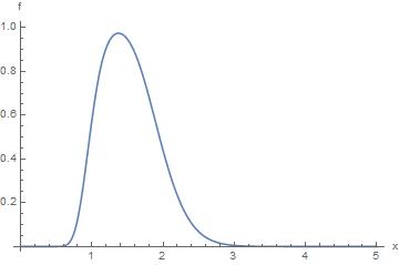
Refer to caption
Refer to caption
Refer to caption
Figure 1. Density f1N(x,t)superscriptsubscript𝑓1𝑁𝑥𝑡f_{1}^{N}(x,t) for N=1𝑁1N=1 (up left), N=2𝑁2N=2 (up right) and N=3𝑁3N=3 (down) at the point t=0.5𝑡0.5t=0.5. Example 3.1.
Refer to caption
Figure 2. Density f1N(x,t)superscriptsubscript𝑓1𝑁𝑥𝑡f_{1}^{N}(x,t) for N=2𝑁2N=2, x𝑥x\in\mathbb{R} and 0t10𝑡10\leq t\leq 1. Example 3.1.
Refer to caption
Refer to caption
Figure 3. Density f1(x,t)subscript𝑓1𝑥𝑡f_{1}(x,t) for t=0.5𝑡0.5t=0.5 (left) and three dimensional plot for x𝑥x\in\mathbb{R} and 0t10𝑡10\leq t\leq 1 (right). Example 3.1.
N𝑁N f1N(x,0.5)f1(x,0.5)L()subscriptnormsuperscriptsubscript𝑓1𝑁𝑥0.5subscript𝑓1𝑥0.5superscriptL\|f_{1}^{N}(x,0.5)-f_{1}(x,0.5)\|_{\mathrm{L}^{\infty}(\mathbb{R})}
111 0.06873430.06873430.0687343
222 0.007434750.007434750.00743475
333 0.003327280.003327280.00332728
Table 1. Error with respect to the exact density function f1(x,t)subscript𝑓1𝑥𝑡f_{1}(x,t) given by (3.1) for N=1𝑁1N=1, N=2𝑁2N=2 and N=3𝑁3N=3, at t=0.5𝑡0.5t=0.5. Example 3.1.
Example 3.2.

Again, consider the homogeneous linear differential equation (b=0𝑏0b=0) with x0Uniform(1,2)similar-tosubscript𝑥0Uniform12x_{0}\sim\text{Uniform}(1,2), but now a𝑎a will not be a Gaussian process. We consider

a(t,ω)=j=12jsin(jπt)ξj(ω),𝑎𝑡𝜔superscriptsubscript𝑗12𝑗𝑗𝜋𝑡subscript𝜉𝑗𝜔a(t,\omega)=\sum_{j=1}^{\infty}\frac{\sqrt{2}}{j}\sin(j\pi t)\xi_{j}(\omega),

where [t0,T]=[0,1]subscript𝑡0𝑇01[t_{0},T]=[0,1] and ξ1,ξ2,subscript𝜉1subscript𝜉2\xi_{1},\xi_{2},\ldots are independent random variables with common density function fξ1(ξ1)=2/(π(1+ξ14))subscript𝑓subscript𝜉1subscript𝜉12𝜋1superscriptsubscript𝜉14f_{\xi_{1}}(\xi_{1})=\sqrt{2}/(\pi(1+\xi_{1}^{4})). These random variables have zero expectation and unit variance, so we have a proper expansion for a𝑎a (its Karhunen-Loève expansion).

We want to approximate the probability density function of the solution process x(t,ω)𝑥𝑡𝜔x(t,\omega) given in (2.14). The assumptions of Theorem 2.8 hold, because fξ1subscript𝑓subscript𝜉1f_{\xi_{1}} is a Lipschitz function on \mathbb{R} (hypothesis H3) and ϕ1(t)=2sin(tπ)>0subscriptitalic-ϕ1𝑡2𝑡𝜋0\phi_{1}(t)=\sqrt{2}\,\sin(t\pi)>0 on (0,1)01(0,1) (hypothesis H4). Hence, (2.16) is a suitable approximation of the density of the process x(t,ω)𝑥𝑡𝜔x(t,\omega) given in (2.14). In Figure 4, we can see f1N(x,t)superscriptsubscript𝑓1𝑁𝑥𝑡f_{1}^{N}(x,t) for N=1𝑁1N=1 (up left), N=2𝑁2N=2 (up right) and N=3𝑁3N=3 (down) at t=0.7𝑡0.7t=0.7. In Figure 5, a three dimensional plot gives f1N(x,t)superscriptsubscript𝑓1𝑁𝑥𝑡f_{1}^{N}(x,t) for N=2𝑁2N=2, x𝑥x\in\mathbb{R} and 0t10𝑡10\leq t\leq 1. In Table 2 we have written the difference between two consecutive orders of truncation N𝑁N at t=0.7𝑡0.7t=0.7. Observe that these differences decrease to 00, which agrees with the theoretical results.

Refer to caption
Refer to caption
Refer to caption
Figure 4. Density f1N(x,t)superscriptsubscript𝑓1𝑁𝑥𝑡f_{1}^{N}(x,t) for N=1𝑁1N=1 (up left), N=2𝑁2N=2 (up right) and N=3𝑁3N=3 (down) at the point t=0.7𝑡0.7t=0.7. Example 3.2.
N𝑁N f1N(x,0.7)f1N+1(x,0.7)L()subscriptnormsuperscriptsubscript𝑓1𝑁𝑥0.7superscriptsubscript𝑓1𝑁1𝑥0.7superscriptL\|f_{1}^{N}(x,0.7)-f_{1}^{N+1}(x,0.7)\|_{\mathrm{L}^{\infty}(\mathbb{R})}
111 0.0107640.0107640.010764
222 0.0001770.0001770.000177
Table 2. Error between two consecutive orders of truncation N𝑁N and N+1𝑁1N+1, for N=1𝑁1N=1 and N=2𝑁2N=2, at t=0.7𝑡0.7t=0.7. Example 3.2.
Refer to caption
Figure 5. Density f1N(x,t)superscriptsubscript𝑓1𝑁𝑥𝑡f_{1}^{N}(x,t) for N=2𝑁2N=2, x𝑥x\in\mathbb{R} and 0t10𝑡10\leq t\leq 1. Example 3.2.
Example 3.3.

Consider the homogeneous linear differential equation (b=0𝑏0b=0) with x0Beta(5,6)similar-tosubscript𝑥0Beta56x_{0}\sim\text{Beta}(5,6), [t0,T]=[0,1]subscript𝑡0𝑇01[t_{0},T]=[0,1] and

a(t,ω)=1+j=12jsin(jπt)ξj(ω),𝑎𝑡𝜔1superscriptsubscript𝑗12𝑗𝑗𝜋𝑡subscript𝜉𝑗𝜔a(t,\omega)=-1+\sum_{j=1}^{\infty}\frac{\sqrt{2}}{j}\sin(j\pi t)\xi_{j}(\omega),

where ξ1,ξ2,subscript𝜉1subscript𝜉2\xi_{1},\xi_{2},\ldots are independent random variables with uniform distribution on (3,3)33(-\sqrt{3},\sqrt{3}) (they have zero expectation and unit variance). Notice that a𝑎a is not a Gaussian process.

The hypotheses of Theorem 2.5 hold, because the density function of a Beta(5,6)Beta56\text{Beta}(5,6) random variable is Lipschitz on \mathbb{R} and 𝔼[ecKa(t,𝝃N)]C𝔼delimited-[]superscripte𝑐subscript𝐾𝑎𝑡subscript𝝃𝑁𝐶\mathbb{E}[\mathrm{e}^{c\,K_{a}(t,\boldsymbol{\xi}_{N})}]\leq C for all n1𝑛1n\geq 1, t[t0,T]𝑡subscript𝑡0𝑇t\in[t_{0},T] and c𝑐c\in\mathbb{R} (see Subsection 2.6). Then (2.16) approximates the density of the process x(t,ω)𝑥𝑡𝜔x(t,\omega) given in (2.14).

In Figure 6, we can see f1N(x,t)superscriptsubscript𝑓1𝑁𝑥𝑡f_{1}^{N}(x,t) for N=1𝑁1N=1 (up left), N=2𝑁2N=2 (up right), N=3𝑁3N=3 (down left) and N=4𝑁4N=4 (down right) at t=0.3𝑡0.3t=0.3. In Figure 7, a three dimensional plot gives f1N(x,t)superscriptsubscript𝑓1𝑁𝑥𝑡f_{1}^{N}(x,t) for N=2𝑁2N=2, x𝑥x\in\mathbb{R} and 0t10𝑡10\leq t\leq 1. To assess analytically the convergence, in Table 3 we show the difference between two consecutive orders of truncation N𝑁N at t=0.3𝑡0.3t=0.3. We observe that these differences decrease to 00, which goes in the direction of our theoretical results.
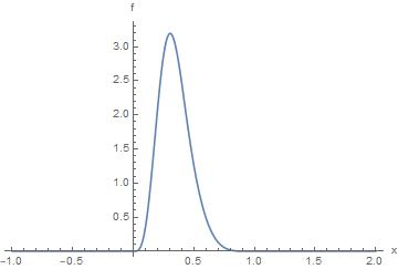
Refer to caption
Refer to caption
Refer to caption
Refer to caption
Figure 6. Density f1N(x,t)superscriptsubscript𝑓1𝑁𝑥𝑡f_{1}^{N}(x,t) for N=1𝑁1N=1 (up left), N=2𝑁2N=2 (up right), N=3𝑁3N=3 (down left) and N=4𝑁4N=4 (down right) at the point t=0.3𝑡0.3t=0.3. Example 3.3.
N𝑁N f1N(x,0.3)f1N+1(x,0.3)L()subscriptnormsuperscriptsubscript𝑓1𝑁𝑥0.3superscriptsubscript𝑓1𝑁1𝑥0.3superscriptL\|f_{1}^{N}(x,0.3)-f_{1}^{N+1}(x,0.3)\|_{\mathrm{L}^{\infty}(\mathbb{R})}
111 0.2253330.2253330.225333
222 0.07996020.07996020.0799602
333 0.02031430.02031430.0203143
Table 3. Error between two consecutive orders of truncation N𝑁N and N+1𝑁1N+1, for N=1𝑁1N=1, N=2𝑁2N=2 and N=3𝑁3N=3, at t=0.3𝑡0.3t=0.3. Example 3.3.
Refer to caption
Figure 7. Density f1N(x,t)superscriptsubscript𝑓1𝑁𝑥𝑡f_{1}^{N}(x,t) for N=2𝑁2N=2, x𝑥x\in\mathbb{R} and 0t10𝑡10\leq t\leq 1. Example 3.3.
Example 3.4.

Consider a complete linear differential equation with x0Normal(0,1)similar-tosubscript𝑥0Normal01x_{0}\sim\text{Normal}(0,1), a(t,ω)=W(t,ω)𝑎𝑡𝜔𝑊𝑡𝜔a(t,\omega)=W(t,\omega) a standard Brownian motion on [0,1]01[0,1] and b(t,ω)𝑏𝑡𝜔b(t,\omega) a standard Brownian bridge on [0,1]01[0,1]:

a(t,ω)=j=12(j12)πsin(t(j12)π)ξj(ω),b(t,ω)=i=12iπsin(tiπ)ηi(ω),formulae-sequence𝑎𝑡𝜔superscriptsubscript𝑗12𝑗12𝜋𝑡𝑗12𝜋subscript𝜉𝑗𝜔𝑏𝑡𝜔superscriptsubscript𝑖12𝑖𝜋𝑡𝑖𝜋subscript𝜂𝑖𝜔a(t,\omega)=\sum_{j=1}^{\infty}\frac{\sqrt{2}}{\left(j-\frac{1}{2}\right)\pi}\sin\left(t\left(j-\frac{1}{2}\right)\pi\right)\xi_{j}(\omega),\quad b(t,\omega)=\sum_{i=1}^{\infty}\frac{\sqrt{2}}{i\pi}\sin\left(ti\pi\right)\eta_{i}(\omega),

where ξ1,ξ2,,η1,η2,subscript𝜉1subscript𝜉2subscript𝜂1subscript𝜂2\xi_{1},\xi_{2},\ldots,\eta_{1},\eta_{2},\ldots are independent and Normal(0,1)Normal01\text{Normal}(0,1) distributed random variables (see Example 5.30 and Exercise 5.12 in [16, p. 204 and p. 216, resp.]).

The hypotheses of Theorem 2.4 hold (see Subsection 2.6). Therefore, the density f1N(x,t)superscriptsubscript𝑓1𝑁𝑥𝑡f_{1}^{N}(x,t) given in (2.5) is an approximation of the density function of the process x(t,ω)𝑥𝑡𝜔x(t,\omega) given in (1.3).

In Figure 8 we have plotted f1N(x,t)superscriptsubscript𝑓1𝑁𝑥𝑡f_{1}^{N}(x,t) for N=1𝑁1N=1, N=2𝑁2N=2 and N=3𝑁3N=3 at t=0.5𝑡0.5t=0.5.

Refer to caption
Refer to caption
Refer to caption
Figure 8. Density f1N(x,t)superscriptsubscript𝑓1𝑁𝑥𝑡f_{1}^{N}(x,t) for N=1𝑁1N=1 (up left), N=2𝑁2N=2 (up right) and N=3𝑁3N=3 (down) at the point t=0.5𝑡0.5t=0.5. Example 3.4.
Example 3.5.

Consider a complete linear differential equation with initial condition x0Gamma(4,9)similar-tosubscript𝑥0Gamma49x_{0}\sim\text{Gamma}(4,9) (444 is the shape and 999 is the rate), domain [t0,T]=[0,1]subscript𝑡0𝑇01[t_{0},T]=[0,1],

a(t,ω)=j=12j3sin(tjπ)ξj(ω),b(t,ω)=i=12i4+6sin(tiπ)ηi(ω),formulae-sequence𝑎𝑡𝜔superscriptsubscript𝑗12superscript𝑗3𝑡𝑗𝜋subscript𝜉𝑗𝜔𝑏𝑡𝜔superscriptsubscript𝑖12superscript𝑖46𝑡𝑖𝜋subscript𝜂𝑖𝜔a(t,\omega)=\sum_{j=1}^{\infty}\frac{\sqrt{2}}{j^{3}}\sin\left(tj\pi\right)\xi_{j}(\omega),\quad b(t,\omega)=\sum_{i=1}^{\infty}\frac{\sqrt{2}}{i^{4}+6}\sin\left(ti\pi\right)\eta_{i}(\omega),

where ξ1,ξ2,,η1,η2,subscript𝜉1subscript𝜉2subscript𝜂1subscript𝜂2\xi_{1},\xi_{2},\ldots,\eta_{1},\eta_{2},\ldots are independent with distribution ξjUniform(3,3)similar-tosubscript𝜉𝑗Uniform33\xi_{j}\sim\text{Uniform}(-\sqrt{3},\sqrt{3}) and ηjNormal(0,1)similar-tosubscript𝜂𝑗Normal01\eta_{j}\sim\text{Normal}(0,1), j1𝑗1j\geq 1.

The assumptions of Theorem 2.4 hold (see Subsection 2.6). Hence, the density f1N(x,t)superscriptsubscript𝑓1𝑁𝑥𝑡f_{1}^{N}(x,t) from (2.5) approximates the density function of the stochastic process x(t,ω)𝑥𝑡𝜔x(t,\omega) given in (1.3).

In Figure 9 we have represented f1N(x,t)superscriptsubscript𝑓1𝑁𝑥𝑡f_{1}^{N}(x,t) for N=1𝑁1N=1 and N=2𝑁2N=2 at t=0.4𝑡0.4t=0.4.

Refer to caption
Refer to caption
Figure 9. Density f1N(x,t)superscriptsubscript𝑓1𝑁𝑥𝑡f_{1}^{N}(x,t) for N=1𝑁1N=1 (left) and N=2𝑁2N=2 (right) at the point t=0.4𝑡0.4t=0.4. Example 3.5.

4. Conclusions

In this paper we have determined approximations for the probability density function of the solution to the randomized non-autonomous complete linear differential equation. This solution is a stochastic process expressed by means of Lebesgue integrals of the data stochastic processes, therefore its probability density function cannot be obtained in an exact manner and approximations for it are required.

The main ideas of this paper can be summarized as follows. Using Karhunen-Loève expansions of the data stochastic processes and truncating them, we obtained a truncation of the solution stochastic process. The Random Variable Transformation technique permitted us to obtain the exact probability density function of the truncation process, which, intuitively, approximates the density function of the solution stochastic process. Theorems 2.4, 2.5, 2.7 and 2.8 give the conditions under which the approximations constructed via these truncations converge uniformly, while Theorems 2.9, 2.10, 2.11, 2.12 and 2.13 give conditions for pointwise convergence. Theorem 2.5, Theorem 2.8, Theorem 2.10, Theorem 2.11 and Theorem 2.13 deal with the non-autonomous homogeneous linear differential equation, which give interesting and particular results when there is no source term in the random differential equation.

It is remarkable that, depending on the way the Random Variable Transformation technique is applied (which variable is essentially isolated when computing the inverse of the transformation mapping), we get different but equivalent expressions for the probability density function of the truncation process. This permitted us to have different hypotheses (theorems) under which the approximating density functions converge. Hence, the generality achieved in terms of applications is notable, as our numerical examples illustrated.

In the numerical experiments we dealt with both Gaussian and non-Gaussian data stochastic processes for which their Karhunen-Loève expansion is available. It was evinced that the convergence to the probability density function of the solution process is achieved quickly.

Acknowledgements

This work has been supported by the Spanish Ministerio de Economía y Competitividad grant MTM2013-41765-P.

Conflicts of interest

None.

References

  • [1] Werner Ebeling and Igor M. Sokolov. Statistical Thermodynamics and Stochastic Theory of Nonequilibrium Systems. Series on Advances in Statistical Mechanics, vol.8. World Scientific, Singapore, 2005. ISBN: 9810213824.
  • [2] Paul H. Wirsching, Thomas L. Paez and Keith Ortiz. Random Vibrations: Theory and Practice. Dover Books on Physics, New York, 2006. ISBN: 0486450155.
  • [3] Linda J.S. Allen. An Introduction to Stochastic Processes with Applications to Biology. Pearson/Prentice Hall, New York, 2010. ISBN: 9780130352187.
  • [4] Bernt Øksendal. Stochastic Differential Equations. An Introduction with Applications. Springer-Verlag, Series: Stochastic Modelling and Applied Probability 23, Heidelberg and New York, 2003.
  • [5] Peter Kloeden and Eckhard Platen. Numerical Solution of Stochastic Differential Equations. Springer-Verlag, Berlin and Heidelberg, 2011.
  • [6] T.T. Soong. Random Differential Equations in Science and Engineering. Academic Press, New York, 1973. ISBN: 0127021507.
  • [7] Ralph C. Smith. Uncertainty Quantification. Theory, Implementation and Applications. SIAM Computational Science & Engineering, SIAM, Philadelphia, 2014. ISBN: 9781611973211.
  • [8] Athanasios Papoulis and S. Unnikrishna Pillai. Probability, Random Variables and Stochastic Processes. McGraw-Hill Europe, 4th edition, 2002. ISBN: 9780071226615.
  • [9] F.A. Dorini, M.S. Cecconello and L.B. Dorini. On the logistic equation subject to uncertainties in the environmental carrying capacity and initial population density. Communications in Nonlinear Science and Numerical Simulation 33 (2016) 160–173. doi:10.1016/j.cnsns.2015.09.009.
  • [10] M.-C. Casabán, J.-C. Cortés, J.-V. Romero and M.-D. Roselló. Probabilistic solution of random SI-type epidemiological models using the Random Variable Transformation technique. Communications in Nonlinear Science and Numerical Simulation 24(1-3) (2014) 86–97. doi:10.1016/j.cnsns.2014.12.016.
  • [11] F.A. Dorini and M. Cristina C. Cunha. Statistical moments of the random linear transport equation. Journal of Computational Physics 227(19) (2008) 8541–8550. doi:10.1016/j.jcp.2008.06.002.
  • [12] A. Hussein and M.M. Selim. Solution of the stochastic radiative transfer equation with Rayleigh scattering using RVT technique. Applied Mathematics and Computation 218(13) (2012) 7193–7203. doi:10.1016/j.amc.2011.12.088.
  • [13] A. Hussein and M.M. Selim. Solution of the stochastic generalized shallow-water wave equation using RVT technique. European Physical Journal Plus (2015) 130:249. doi:10.1140/epjp/i2015-15249-3.
  • [14] A. Hussein and M.M. Selim. A general analytical solution for the stochastic Milne problem using Karhunen-Loève (K-L) expansion. Journal of Quantitative Spectroscopy and Radiative Transfer 125 (2013) 84–92. doi:10.1016/j.jqsrt.2013.03.018.
  • [15] Zhijie Xu, Ramakrishna Tipireddy and Guang Lin. Analytical approximation and numerical studies of one-dimensional elliptic equation with random coefficients. Applied Mathematical Modelling 40(9-10) (2016) 5542-5559. doi:10.1016/j.apm.2015.12.041.
  • [16] Gabriel J. Lord, Catherine E. Powell and Tony Shardlow. An Introduction to Computational Stochastic PDEs. Cambridge Texts in Applied Mathematics, Cambridge University Press, New York, 2014. ISBN: 9780521728522.
  • [17] M.-C. Casabán, J.-C. Cortés, J.-V. Romero and M.-D. Roselló. Determining the first probability density function of linear random initial value problems by the random variable transformation (RVT) technique: a comprehensive study. Abstract and Applied Analysis 2014–ID248512 (2014) 1–25. doi:10.1155/2013/248512.
  • [18] M.-C. Casabán, J.-C. Cortés, J.-V. Romero and M.-D. Roselló. Solving Random Homogeneous Linear Second-Order Differential Equations: A Full Probabilistic Description. Mediterranean Journal of Mathematics 13(6) (2016) 3817–3836. doi:10.1016/10.1007/s00009-016-0716-6.
  • [19] J.-C. Cortés, A. Navarro-Quiles, J.-V. Romero and M.-D. Roselló. Probabilistic solution of random autonomous first-order linear systems of ordinary differential equations. Romanian Reports in Physics 68(4) (2016) 1397–1406.
  • [20] Elias M. Stein and Rami Shakarchi. Real Analysis: Measure Theory, Integration, and Hilbert Spaces. Princeton Lectures in Analysis III, Princeton University Press, 2005. ISBN: 9780691113869.
  • [21] Walter Rudin. Principles of Mathematical Analysis. International Series in Pure & Applied Mathematics, third edition, 1976. ISBN: 9780070542358.
  • [22] David Williams. Probability with Martingales. New York, Cambridge University Press, 1991. ISBN: 9780521406055.
  • [23] Alan J. Weir. Lebesgue integration and measure. Cambridge University Press, 1973. ISBN: 9780521097512.
  • [24] Athreya, Krishna B. and Lahiri, Soumendra N.. Measure theory and probability theory. Springer, 2006. ISBN: 9780387329031.
  • [25] Hale, Jack K.. Ordinary Differential Equations. Malabar: Robert E. Krieger Publishing Company, Second edition, 1980. ISBN: 9780486472119.
  • [26] Pascal Massart. Concentration Inequalities and Model Selection. Ecole d’Eté de Probabilités de Saint-Flour XXXIII - 2003, Springer, 2007. ISBN: 9783540485032.
  • [27] Samuel Karlin. The existence of eigenvalues for integrals operators. Transactions of the American Mathematical Society, Vol. 113, No. 1 (Oct., 1964), pp. 1-17.
  • [28] Roger A. Horn and Charles R. Johnson. Matrix Analysis. Cambridge University Press, second edition, 1985. ISBN: 9780521548236.
  • [29] Sandro Salsa. Partial Differential Equations in Action From Modelling to Theory. Springer, 2009. ISBN: 9788847007512.
  • [30] Tigran Harutyunyan, Avetik Pahlevanyan and Yuri Ashrafyan. On the movement of the zeros of eigenfunctions of the Sturm-Liouville problem. Proceedings of Artsakh State University, (2013), No. 1(27), pp. 12-20.
  • [31] Jordan M. Stoyanov. Counterexamples in Probability. Dover publications, third edition, 2013. ISBN: 9780486499987.
  • [32] D. Xiu. Numerical Methods for Stochastic Computations. A Spectral Method Approach. Cambridge Texts in Applied Mathematics, Princeton University Press, New York, 2010. ISBN: 9780691142128.