A semi-analytical approach to black body radiation

Abstract

We describe a semi-analytical method to calculate the total radiance received form a black body, between two frequencies. As has been done before, the method takes advantage of the fact that the solution simplifies with the use of polylogarithm functions. We then use it to study the amount of radiation from the sun received by bodies at Earths surface.

Keywords: Black body radiation, Available energy, Polylogarithm

1 Introduction

What follows started originally as a question in a second year undergraduate course on Modern Physics. The question was simple: We know the Boltzmann formula for the total radiation of a black body, but what is total radiance between two particular wavelengths. It was posed by the instructor as an assignment, but the students took it to heart, completing a long and interesting path researching what they now know to be Planck integrals and the Polylogarithm functions. Our intention here is to highlight the main points learned, in an effort to make it accessible to other undergraduate students.

A black body is an ideal theoretical object which absorbs all the energy that falls on its surface as light. There is no reflection nor light passing through the black body. Due to the nature of radiation absorption, which can be modelled as the resonance of charge at the surface of the body, black bodies can actually emit all the energy as light, given enough time, again in all wave lengths or frequencies (see e.g. [1]).

Perfect black bodies seldom occur naturally, even black smoke reflects up to $1\%$ of the incident light. The name black body was first introduced by Gustav Kirchhoff in the 1860’s. The emitted light of one of these objects is called black body radiation; despite its name, it constitutes a physical model for studying the emission of electromagnetic radiation of solids or liquids.

This radiation refers, therefore, to the continuous energy emission from the surface of any body, which is transported by means of electromagnetic waves that can travel in the vacuum at the speed of light. The radiant energy emitted from a body at room temperature is small and corresponds to wavelengths greater than those of visible light (lower frequency). With increasing temperature the emitted energy increases and the wavelengths become shorter. This is the reason we see a change in the colour of a body when heated. Bodies do not emit with the same intensity in all frequencies or wavelengths, a good model for this intensity is Planck’s law for black body radiation, which is a function of the body’s temperature[2]. The emitted energy of a solid also depends on the nature of its surface; we can then have a matte or black surface with larger emission power than that of a glossy one. The energy emitted by an incandescent charcoal filament is larger than that of a platinum filament at the same temperature. Therefore, real bodies will emit radiation with varying efficiency (a concept known as emissivity), in these cases the well known black body spectra must be adapted to give more realistic answers (see e.g. Ramírez-Moreno et al. [3], and references therein). The surface of a black body is the limiting case in which all the light from the exterior is absorbed and all the interior energy is emitted[4].

We may find the theoretical model for black body radiation in any introductory text on Modern Physics. The expression for the energy of the radiation in an interval ${\rm d}\nu$ is a rather simple relation and it turns out that this density is proportional to the total radiance emitted by the black body[5]. However, if we are to calculate the total energy between two frequencies $\nu_{1}$ and $\nu_{2}$ we must use special functions or implement some numerical technique.

The importance of radiation absorption and emission has lead to the study of black body radiation for many years and in many fields. A report on an exact solution, written as an infinite series, can be found in the work by S.L. Chang and K.T. Rhee[6]. A very complete discussion of how this solution may be rewritten in terms of polylogarithms is discussed by Seán M. Stewart[7]. Although developed in an independent way, we will build on these ideas and implement the functions numerically for particular ranges in wavelength. The subject of integrating black body radiation in a particular range of wavelength is also known as band emission and has been extensively discussed by the infrared imaging community (see e.g. Vollmer and Möllmann[8] and references therein).

In this work We take data from recent radiation measurements and aim to implement a semi-analytical approach for calculating the fraction of radiation from the Sun that is available at ground level. These estimates may be important for recent applications in renewable energy sources for calculating the total radiance available to solar panels and may be easily adapted for each region for which the radiance map is known (or may be measured).

The paper is organised as follows: after this brief introduction, section 2 presents the semi-analytical technique, in section 3 we apply it to some generic data and our results are summarised in the conclusions.

2 Energy density between two frequencies.

The full description for black body radiation was not realised until 1900 when, almost reluctantly, Max Planck was able to construct an expression that reproduced all of the data (unlike the previous intents by Lord Rayleigh and Sir James Jeans, for low frequencies and Wien and Planck for higher frequencies[9]) .

The details of these developments can be found in many textbooks on modern physics (eg, [1, 10]). The description centres on considering a cavity with metallic walls heated uniformly to temperature $T$. The walls emit electromagnetic radiation in the thermal range of frequencies. Rayleigh and Jeans used classic electromagnetic theory to demonstrate that the radiation in the interior of the cavity must exists as standing waves whose nodes correspond to the metallic surfaces. In the classic theory, the average of total energy only depends on temperature $T$. The number of standing waves in the frequency interval times the average energy of these waves, divided by the volume of the cavity, gives the average energy content per unit volume in the frequency interval between $\nu$ and $\nu+{\rm d}\nu$. This is the required quantity: the energy density $\rho_{T}(\nu)$. By considering that these standing waves contained in the cavity must have discrete energy values, we may write the expression for the spectral energy density:

$$\rho(\nu){\rm d}\nu=\frac{8\pi{\rm h}}{\rm c^{3}}\frac{\nu^{3}}{{\rm e}^{\frac{\rm h\nu}{{\rm k}T}}-1}{\rm d}\nu$$

and then obtain the spectral radiance of the body as a multiple of this density[5]:

$$R(\nu){\rm d}\nu=\frac{c}{4}\rho(\nu){\rm d}\nu$$ (1)

This quantity is defined as the energy radiated per unit length per unit time in a frequency interval ${\rm d}\nu$. We illustrate this radiance for three distinct temperature values $T_{1}<T_{2}<T_{3}$ in figure 1 (throughout this paper we use the usual notation for the Planck constant, ${\rm h}$, the speed of light in the vacuum, ${\rm c}$, and the Boltzmann constant, ${\rm k}$).

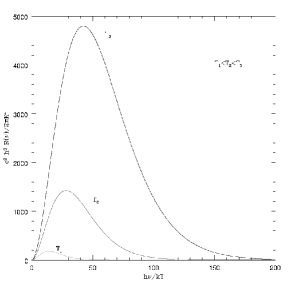
Figure 1: Spectral radiance for a body at three temperature values, $T_{1}<T_{2}<T_{3}$. As— temperature increases, the maximum of the curve moves to higher frequencies and the radiance is significant for a greater interval of frequencies.

2.1 Energy density and polylogarithms

Once we know the expression for the spectral energy density of a black body it is not difficult to integrate the total energy per unit volume available between two specific frequencies, $\nu_{a}$ and $\nu_{b}$:

$$\rho_{ab}(T)\equiv\int_{\nu_{a}}^{\nu_{a}}\rho(\nu){\rm d}\nu=\int_{\nu_{a}}^{\nu_{b}}\frac{\rm 8\pi h}{c^{3}}\frac{\nu^{3}}{{\rm e}^{\frac{\rm h\nu}{{\rm k}T}}-1}{\rm d}\nu$$ (2)

Since the two frequencies between-which we would like to calculate the energy density are constant, the quantity that we have just defined in equation (2) is only a function of the temperature of the black body (i.e. we will treat $\nu_{a}$ and $\nu_{b}$ as parameters). Of particular importance and historical significance is $\rho_{0\infty}(T)\equiv\rho_{T}(T)$ which is the total energy density of the black body, integrated over all frequencies, we will get back to this integral as a specific case of the the general expression between two frequencies.

In order to handle the integral more easily, we suggest using the following adimensional variables :

$$\begin{array}[]{ccccc}\chi=\frac{\rm h\nu}{{\rm k}T}&&{\rm and}&&\rho(\chi){\rm d}\chi=\frac{8\pi{{\rm k}^{4}T^{4}}}{\rm c^{3}h^{3}}\tilde{\rho}(\chi){\rm d}\chi\end{array}$$

using these definitions, we can calculate the total energy density of the black body between two frequencies, $\nu_{a}$ and $\nu_{b}$.

Before we continue, as we shall soon encounter, the spectral range for radiation is commonly given in wavelengths, rather than frequencies. We have written 2 because this form will turn out to be useful for our analytical manipulation. Let us consider for a moment that, instead of a frequency range, we have a wavelength range, which corresponds to the same physical range for the radiation; in this case the energy density of interest is

$$\rho_{ab}(T)=\int_{\lambda_{a}}^{\lambda_{b}}\rho(\lambda){\rm d}\lambda$$

which we would use if the spectral density is a function of wavelength. Now, let us examine this integral, we could split this problem into a couple of integrals:

$$\rho_{ab}(T)=\int_{o}^{\lambda_{b}}\rho(\lambda){\rm d}\lambda-\int_{o}^{\lambda_{a}}\rho(\lambda){\rm d}\lambda$$

if we further consider the specific form for $\rho(\lambda)$, and change from wavelength to frequency, it turns out that[11]

$$\int_{o}^{\lambda_{o}}\rho(\lambda){\rm d}\lambda=\int_{\nu_{o}}^{\infty}\tilde{\rho}(\chi){\rm d}\chi$$

where the specific frequency, $\nu_{o}$, and wavelength, $\lambda_{o}$, are related, in the usual way, through the speed of light in the vacuum: $c=\nu_{o}\lambda_{o}$.

In this way we may do the integral over a wavelength range by using the equivalent frequency, and again splitting the problem into a couple of integrals:

$$\rho_{ab}(T)=\beta\left[\int_{\chi_{b}}^{\infty}\tilde{\rho}(\chi){\rm d}\chi-\int_{\chi_{a}}^{\infty}\tilde{\rho}(\chi){\rm d}\chi\right],$$

notice that all the physical units have been accounted for in the temperature parameter $\beta=\frac{8\pi{\rm k}^{4}T^{4}}{\rm c^{3}h^{3}}$. If we define the following auxiliary function:

$$F(\chi)=\int_{\chi}^{\infty}\frac{\chi^{\prime 3}}{{\rm e}^{\chi^{\prime}}-1}{\rm d}\chi^{\prime}$$ (3)

the required energy density is then:

$$\rho_{ab}(T)=\beta\left[F(\chi_{b})-F(\chi_{a})\right]$$ (4)

with the frequencies written as $\chi_{i}=\frac{\rm h\nu_{i}}{{\rm k}T}$

To solve $F(\chi)$ we study the integrand and notice that it looks like the convergence of a geometric series; this leads us to factorise ${\rm e}^{\chi}$ and write the integrand as:

$$\frac{\chi^{3}}{{\rm e}^{\chi}-1}=\chi^{3}{\rm e}^{-\chi}\cdot\left[\frac{1}{1-{\rm e}^{-\chi}}\right]$$

In this last expression we recognise the geometrical series as the value between brackets. Because we will consider only values $\nu>0$, for which $\chi>0$, we can then rewrite the integrand as follows:

$$\frac{\chi^{3}}{{\rm e}^{\chi}-1}=\sum_{n=0}^{\infty}\chi^{3}{\rm e}^{-(n+1)\chi}$$

The function $F(\chi)$ then becomes:

$$F(\chi)=\sum_{n=0}^{\infty}\int_{\chi}^{\infty}\chi^{\prime 3}{\rm e}^{-(n+1)\chi^{\prime}}{\rm d}\chi^{\prime}$$

We integrate the right hand side of this last expression: first we integrate by parts three times to reduce the exponent of $\chi$, then we evaluate the resulting expressions, noticing that many terms vanish for $\chi\rightarrow\infty$. After cleaning up the expression we can write the result as follows:

$$F(\chi)=\sum_{n=0}^{\infty}\frac{{\rm e}^{-(n+1)\chi}}{n+1}\left[\chi^{3}+\frac{3\chi^{2}}{(n+1)}+\frac{6\chi}{(n+1)^{2}}+\frac{6}{(n+1)^{3}}\right]$$

In this last expression, we can change the index, $(n+1)\rightarrow n$, so that $F$ is written in its most compact form:

$$F(\chi)=\sum_{n=1}^{\infty}\frac{{\rm e}^{-n\chi}}{n}\left[\chi^{3}+\frac{3\chi^{2}}{n}+\frac{6\chi}{n^{2}}+\frac{6}{n^{3}}\right]$$ (5)

To prove convergence of 5 we use the ratio test, which guarantees that a series $\sum_{n=1}^{\infty}S_{n}$ converges when it meets the following condition

$$L=\lim_{n\rightarrow\infty}|\frac{S_{n+1}}{S_{n}}|<1$$

For this particular case we have:

$$\frac{S_{n+1}}{S_{n}}=\frac{\frac{{\rm e}^{(n+1)\chi}}{n+1}}{\frac{{\rm e}^{-n\chi}}{n}}\left[\frac{\chi^{3}+\frac{3\chi^{2}}{n+1}+\frac{6\chi}{(n+1)^{2}}+\frac{6}{(n+1)^{3}}}{\chi^{3}+\frac{3\chi^{2}}{n}+\frac{6\chi}{n^{2}}+\frac{6}{n^{3}}}\right]$$

rearranging terms and taking the limit

$$L=\lim_{n\rightarrow\infty}\frac{n{\rm e}^{-(n+1)\chi}}{(n+1){\rm e}^{-n\chi}}\left[\frac{\chi^{3}+\frac{3\chi^{2}}{n+1}+\frac{6\chi}{(n+1)^{2}}+\frac{6}{(n+1)^{3}}}{\chi+\frac{3\chi^{2}}{n}+\frac{6\chi}{n^{2}}+\frac{6}{n^{3}}}\right]=\frac{1}{{\rm e}^{\chi}}$$

Because we are only interested in cases where $\nu>0$ and therefore $\chi=\frac{\rm h\nu}{{\rm k}T}>0$, $L<1$ and the series converges for all possible values in which we will use our auxiliary function. Thus, we may now write the integrated energy density as:

$$\int_{\nu}^{\infty}\rho{(\nu^{\prime})}d\nu^{\prime}=\beta F(\chi)=\beta\sum_{n=1}^{\infty}\frac{{\rm e}^{-n\chi}}{n}\left[\chi^{3}+\frac{3\chi^{2}}{n}+\frac{\chi}{n^{2}}+\frac{6}{n^{3}}\right]$$ (6)

For any particular frequency $\nu$, written as $\chi=\frac{h\nu}{kT}$, and temperature, $\beta=\frac{8\pi k^{4}T^{4}}{c^{3}h^{3}}$.

To recover the the energy density we need to evaluate $F(\chi)$. For this purpose we must quantify the following four sums:

$$\begin{array}[]{ccc}F_{1}(\chi)=\chi^{3}\sum_{n=1}^{\infty}\frac{({\rm e}^{-\chi})^{n}}{n}&&F_{2}(\chi)=3\chi^{2}\sum_{n=1}^{\infty}\frac{({\rm e}^{-\chi})^{n}}{n^{2}}\\ \\ F_{3}(\chi)=6\chi\sum_{n=1}^{\infty}\frac{({\rm e}^{-\chi})^{n}}{n^{3}}&&F_{4}(\chi)=6\sum_{n=1}^{\infty}\frac{({\rm e}^{-\chi})^{n}}{n^{4}}\end{array}$$

In the first sum, we identify the logarithm series:

$$\ln(1-Y)=(-1)\sum_{(n=1)}^{\infty}\frac{Y^{n}}{n}\;\;\;\;\mbox{with}\;\;\;\;|Y|<1$$

Identifying ${\rm e}^{-\chi}=Y$, because we will always consider cases such that $\chi>0$, $|Y|<1$ and the first sum can be written as:

$$F_{1}(\chi)=-\chi^{3}\ln(1-{\rm e}^{-\chi})$$

To solve the remaining sums, we identify a special function that arises in Quantum Field Theory, the polylogarithm, ${\rm Li}_{m}$ (see e.g. [12, 13] and references therein):

$${\rm Li}_{m}(z)=\frac{(-1)^{m-1}}{(m-2)!}\int_{0}^{1}\frac{\ln^{m-2}(t)\ln(1-tz)}{t}dt=\sum_{n=1}^{\infty}\frac{z^{n}}{n^{m}}$$

Here we will use these functions, known as Nielsen’s Generalised Polylogarithms[14], which allow us to reduce the problem to a family of integrals. By identifying $z={\rm e}^{-\chi}$, we see that each of the three remaining sums may be related to a specific polylogarithm:

$$\begin{array}[]{ccccc}F_{2}(\chi)&=&3\chi^{2}{\rm Li}_{2}({\rm e}^{-\chi})&=&-3\chi^{2}{\displaystyle\int}_{0}^{1}\frac{\ln(1-t{\rm e}^{-\chi})}{t}dt\\ &&\\ F_{3}(\chi)&=&6\chi{\rm Li}_{3}({\rm e}^{-\chi})&=&6\chi^{2}{\displaystyle\int}_{0}^{1}\frac{\ln(t)\ln(1-t{\rm e}^{-\chi})}{t}dt\\ &&\\ F_{4}(\chi)&=&6{\rm Li}_{4}({\rm e}^{-\chi})&=&-3{\displaystyle\int}_{0}^{1}\frac{\ln^{2}(t)\ln(1-t{\rm e}^{-\chi})}{t}dt\end{array}$$ (7)

This is as far as we can go analytically. The possible values for $\chi$ guarantee that all of the integrals in (7) will converge to a specific value, once we have a range of frequencies. All that remains is to apply a numerical algorithm and we may solve many interesting problems. Two particular cases are discussed in the next section.

3 Examples

With the simple relation in 6 we can now recover physical interesting quantities very easily. We now consider two cases for which the formulation developed leads to quick results. The first is a more analytical example which exemplifies the fundamental nature of black body radiation, while the second is a more applied case for which integrating the parts of the spectrum may be interesting.

3.1 The fundamental constants of black body radiation

Consider the relation between spectral radiance and energy density: G

$$R(\nu)d\nu=\frac{c}{4}\rho(\nu)d\nu$$

Due to the fact that we can measure radiance readily, this quantity is of interest in many fields. Using our auxiliary function, the total radiance, $R_{T}$, of a black body can be calculated from it:

$$R_{T}=\int_{0}^{\infty}R(\nu)d\nu=\frac{c}{4}\int_{0}^{\infty}\rho(\nu)d\nu$$

but, we also know that:

$$R_{T}=\sigma T^{4}$$

then

$$R_{T}=\frac{c}{4}\int_{0}^{\infty}\rho(\nu)d\nu=\sigma T^{4}$$

Using our expression for $F$ we can solve the middle integral easily,

$$R_{T}=\frac{c}{4}F(0)=\sigma T^{4}$$

We see from (6) that $F(0)$ is a constant, in fact:

$$F(0)=\beta\sum_{n=1}^{\infty}\frac{6}{n^{4}}=6\beta\sum_{n=1}^{\infty}n^{-4}=6\beta\zeta(4)$$

in the last step, we have used the Riemann zeta function, defined by:

$$\zeta(s)=\sum_{n=1}^{\infty}n^{-s},\ \ \ \ \ \ \ s>1$$

which converges, and for the case ${\rm s=4}$, has a value of (see, e.g. [15]):

$$\zeta(4)=\frac{\pi^{4}}{90}$$

then ${\rm F(0)=\beta\frac{\pi^{4}}{15}}$ and the total energy density can be written:

$$\rho_{T}=\frac{8\pi^{5}{\rm k}^{4}T^{4}}{15{\rm c^{3}h^{3}}}$$

We have found an expression for the total radiance of a black body.

$$R_{T}=\frac{c}{4}\rho_{T}=\frac{2\pi^{5}{\rm k}^{4}}{15{\rm c^{2}h^{3}}}T^{4}$$

this means that we have found an alternative expression for Stefan’s constant in terms of fundamental quantities:

$$\sigma=\frac{2\pi^{5}{\rm k}^{4}}{15{\rm c^{2}h^{3}}}$$

3.2 The total absorbed radiation at Earths surface

With the current interest in alternative energies, the question of how much energy is available from the sun at earths surface becomes very important for any application that aims at taking advantage of this clean source of energy.

As light from the sun reaches the earth, the atmosphere blocks out considerable parts of the spectrum, in figure 2 we have plotted the amount of radiation which eventually reaches the surface of the earth on a given day, in the southwest USA [16]. In Figure 2 (a) we have plotted in red the standard spectra of the sun as it reaches the atmosphere, while the other two lines show the direct components that reach the earth surface, in blue we show the direct beam from the sun plus the circumsolar component in a disk 2.5 degrees around the sun, while the green is just the direct beam radiation. (although this plot is ours, it is intended to reproduce that shown in the web page mentioned above). We can consider this green line to indicate the total light available to us for collection by ground systems. We also plot a black body curve adjusted to a temperature of 5100K, shown in black, which we use to model the direct beam component.

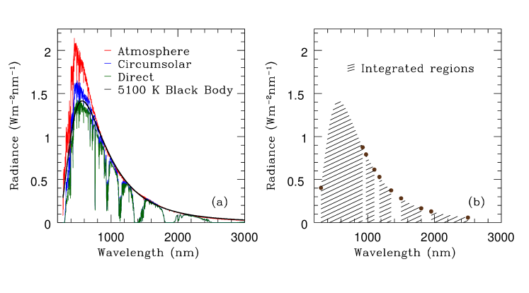
Figure 2: (a) Spectra of the sun: red, as it reaches the atmosphere; blue, direct beam plus circumsolar component in a disk 2.5 degrees around the sun; green, direct beam. In black we plot the corresponding curve of a 5100K black body. (b) Approximation of filtered, direct beam, spectra as it reaches the surface of the earth.

As we can see, the radiation is highly filtered by the atmosphere, so not all wavelengths reach the Earths surface. In Figure 2 (b) we have reproduced the black body fit at 5100K as above, but have now removed part of the spectrum which is naturally filtered. The wavelength intervals (measured in nm) to be integrated are thus: [300.,925.], [975., 1100.], [1175.,1350.], [1500.,1800.] and [1950.,2500.]. To calculate the total radiance available, we will use a modified version of (4) and the relation between spectral radiance and energy density, since we may add each contribution, we can write the total radiance received at the surface:

$$R_{T}=\frac{c}{4}\beta\sum_{i}\left[F(\chi_{b_{i}})-F(\chi_{a_{i}})\right]$$

In this last expression, $\chi_{a_{i}}$ represent the frequencies associated to the initial part of each interval: $\{300.,975.,1175.,1500.,1950.\}$, while $\chi_{b_{i}}$ represent the final part: $\{925.,1100.,1350.,1800.,2500.\}$. Using (6) with the method developed in the past section and a suitable method for numerical integration, we can find the integrated radiance in each of these intervals and thus the total available radiation at the earths surface.

In table 1 we present the value of F for the different wavelengths chosen. If we recall that our temperature parameter $\beta$ is determined by the black body fit to 5100K, then $\beta=2.36289\times 10^{7}$Wm^-2, and this leads us to a total radiation equivalent to:

$$R_{T}=1.24402\times 10^{8}{\rm Wm}^{-2}$$ (8)

$\lambda_{a}$ (nm)	F	$\lambda_{b}$ (nm)	F
300.	0.09554	925.	3.87127
975.	4.09277	1100.	4.55882
1175.	4.78702	1350.	5.20358
1500.	5.46369	1800.	5.81167
1950.	5.92909	2500.	6.1876

Table 1: Auxiliary function, $F$, values for the wavelengths of interest defined in Figure 2

4 Conclusions

We have presented a review of a compact form to calculate the total radiance output from a black body between two wavelengths. Considering modern computational techniques and power, the expressions presented are relatively easy to manage and can lead to quick results.

These results may allow better estimates of the available power for radiance capturing experiments. If we were to model the total radiation at the earths surface by the simple fit to a 5100K black body without considering that there are filtered regions and simply integrate through the whole wavelength range (300 nm to 2500 nm) then the calcultaed radiance obtained in equation 8 would be only slightly more that 87% of the total radiance calculated. Therefore, we beleave that a technique such as the one presented in this work are of special importance if we are to model correctly the available energy.

5 Acknowledgements

The authors would like to acknowledge the generosity of Dr. Christiana Honsberg and Dr. Stuart Bowden at the Solar Power Labs ASU (http://pv.asu.edu/), for making the solar spectra available in an easy to use format at www.pveducation.org. D. Santana and O. Salcido acknowledge the generous support of CONACyT through a grant for postgraduate training. This project was partially supported by a grant from the División de Ciencias Exactas y Naturales of the Universidad de Sonora, grant no: USO315001752.

References

References

- [1] Krane K S 2012 Modern Physics. 3rd ed (John Wiley & Sons, Inc.) ISBN 978-1118061145
- [2] Crepeau J 2008 Josef stefan and his contributions to heat transfer ASME 2008 Heat Transfer Summer Conference vol 3 ed Walsh D American Society of Mechanical Engineers (Two Park Avenue. New York, NY 10016-5990: American Society of Mechanical Engineers) p 669
- [3] Ramírez-Moreno M A, González-Hernández S and Ares de Parga G 2015 Eur. J. Phys. 36 URL http://stacks.iop.org/0143-0807/36/i=6/a=065039
- [4] Poprawski W, Gnutek Z, Radojewska E B and Poprawski R 2015 European Journal of Physics 36 065025 URL http://stacks.iop.org/0143-0807/36/i=6/a=065025
- [5] Zombeck M 2007 Handbook of Space Astronomy and Astrophysics: Third Edition 3rd ed (Cambridge University Press) ISBN 781-0-521-78242-5 URL http://www.astrohandbook.com/ch14/radiation_defs.pdf
- [6] Chang S and Rhee K 1984 International Communications in Heat and Mass Transfer 11 451 – 455 ISSN 0735-1933 URL http://www.sciencedirect.com/science/article/pii/ 0735193384900514
- [7] Stewart S M 2012 Journal of Quantitative Spectroscopy and Radiative Transfer 113 232 – 238 ISSN 0022-4073 URL http://www.sciencedirect.com/science/article/pii/ S0022407311003736
- [8] Vollmer M and Möllmann K P 2011 Infrared Thermal Imaging: Fundamentals, Research and Applications (Wiley-VCH) ISBN 978-3-527-40717-0 URL http://www.wiley.com/WileyCDA/WileyTitle/productCd- 3527407170.html
- [9] Kragh H 2000 Physics World 13 31–35 ISSN 0953-8585
- [10] Eisberg R M and Resnick R 1985 Quantum Physics of Atoms, Molecules, Solids, Nuclei, and Particles (Wiley) ISBN 978-0-471-87373-0
- [11] Michels T E 1968 Planck functions and integrals; methods of computation Tech. rep. National Aeronautics and Space Administration NASA TN D-4446
- [12] Frellesvig H, Tommasini D and Wever C 2016 Journal of High Energy Physics 2016 1–36 ISSN 1029-8479 URL http://dx.doi.org/10.1007/JHEP03(2016)189
- [13] Vollinga J and Weinzierl S 2005 Computer Physics Communications 167 177 – 194 ISSN 0010-4655 URL http://www.sciencedirect.com/science/article/pii/ S0010465505000706
- [14] Kölbig K S 1986 SIAM Journal on Mathematical Analysis 17 1232–1258 URL http://dx.doi.org/10.1137/0517086
- [15] Arfken G B 1985 Mathematical methods for physicists 3rd ed (Academic Press) ISBN 978-0120598205
- [16] Honsberg C and Bowden S Standard Solar Spectra http://www.pveducation.org/pvcdrom/appendices/standard-solar-spectra Accessed: 2017-02-11