On a toy network of neurons interacting through their dendrites

Abstract.

Consider a large number $n$ of neurons, each being connected to approximately $N$ other ones, chosen at random. When a neuron spikes, which occurs randomly at some rate depending on its electric potential, its potential is set to a minimum value $v_{min}$, and this initiates, after a small delay, two fronts on the (linear) dendrites of all the neurons to which it is connected. Fronts move at constant speed. When two fronts (on the dendrite of the same neuron) collide, they annihilate. When a front hits the soma of a neuron, its potential is increased by a small value $w_{n}$. Between jumps, the potentials of the neurons are assumed to drift in $[v_{min},\infty)$, according to some well-posed ODE. We prove the existence and uniqueness of a heuristically derived mean-field limit of the system when $n,N\to\infty$ with $w_{n}\simeq N^{-1/2}$. We make use of some recent versions of the results of Deuschel and Zeitouni [15] concerning the size of the longest increasing subsequence of an i.i.d. collection of points in the plan. We also study, in a very particular case, a slightly different model where the neurons spike when their potential reach some maximum value $v_{max}$, and find an explicit formula for the (heuristic) mean-field limit.

1. Introduction and motivation

Our goal is to establish the existence and uniqueness of the heuristically derived mean-field limits of two closely related toy models of neurons interacting through their dendrites.

1.1. Description of the particle systems

We have $n$ neurons, each has a linear dendrite with length $L>0$ that is endowed with a soma at one of its two extremities. We have some i.i.d. Bernoulli random variables $(\xi_{ij})_{i,j\in\{1,\dots,n\}}$ with parameter $p_{n}\in(0,1)$, as well as some i.i.d. $[0,L]$-valued random variables $(X_{ij})_{i,j\in\{1,\dots,n\}}$ with probability density $H$ on $[0,L]$. If $\xi_{ij}=1$, then the neuron $i$ influences the neuron $j$, and the link is located, on the dendrite of the $j$-th neuron, at distance $X_{ij}$ of its soma.

We have a minimum potential $v_{min}\in{\mathbb{R}}$, an excitation parameter $w_{n}>0$, a regular drift function $F:[v_{min},\infty)\mapsto{\mathbb{R}}$ such that $F(v_{min})\geq 0$, a propagation velocity $\rho>0$ and a delay $\theta\geq 0$.

We denote by $V^{i,n}_{t}$ the electric potential of the $i$-th neuron at time $t\geq 0$. We assume that initially, the random variables $(V^{i,n}_{0})_{i=1,\dots,n}$ are i.i.d. with law $f_{0}\in{\mathcal{P}}([v_{min},\infty))$.

Between jumps (corresponding to spike or excitation events), the membrane potentials of all the neurons satisfy the ODE $(V^{i,n}_{t})^{\prime}=F(V^{i,n}_{t})$. Note that all the membrane potentials remain above $v_{min}$ thanks to the condition $F(v_{min})\geq 0$.

When a neuron spikes (say, the neuron $i$, at time $\tau$), its potential is set to $v_{min}$ (i.e. $V^{i,n}_{\tau}=v_{min})$ and, for all $j$ such that $\xi_{ij}=1$, two fronts start, after some delay $\theta$ (i.e. at time $\tau+\theta$), on the dendrite of the $j$-th neuron, at distance $X_{ij}$ of the soma. Both fronts move with constant velocity $\rho$, one going down to the soma (such a front is called positive front), the other one going away from the soma (such a front is called negative front).

On the dendrite of each neuron, we thus have fronts moving with velocity $\rho$. When a negative front reaches the extremity of the dendrite, it disappears. When a positive front meets a negative front, they both disappear. When finally a positive front hits the soma (say, of the $j$-th neuron at time $\sigma$), the potential of $j$ is increased by $w_{n}$, i.e. $V^{j,n}_{\sigma}=V^{j,n}_{\sigma-}+w_{n}$ and the positive front disappears. Such an occurrence is called an excitation event.

We assume that at time $0$, there is no front on any dendrite. This is not very natural, but considerably simplifies the study.

It remains to describe the spiking events, for which we propose two models.

Soft model. We have an increasing regular rate function $\lambda:[v_{min},\infty)\mapsto{\mathbb{R}}_{+}$. Each neuron (say the $i$-th one) spikes, independently of the others, during $[t,t+dt]$, with probability $\lambda(V^{i,n}_{t})dt$.

Hard model. There is a maximum electric potential $v_{max}>v_{min}$. In such a case, we naturally assume that $f_{0}$ is supported in $[v_{min},v_{max}]$. A neuron spikes each time its potential reaches $v_{max}$. This can happen for two reasons, either due to the drift (because it continuously drives $V^{i,n}_{t}$ to $v_{max}$ at some time $\tau$, i.e. $V^{i,n}_{\tau-}=v_{max}$), or due to an excitation event (we have $V^{i,n}_{\tau-}<v_{max}$, a positive front hits the soma of the $i$-th neuron at time $\tau$ and $V^{i,n}_{\tau}=V^{i,n}_{\tau-}+w_{n}\geq v_{max}$).

Observe that the hard model can be seen as the soft model with the choice $\lambda(v)=\infty{\mathbbm{1}}_{\{v\geq v_{max}\}}$. The soft model is thus a way to regularize the spiking events by randomization. If, as we have in mind, $\lambda$ looks like $\lambda(v)=(\max\{v-v_{0},0\}/(v_{1}-v_{0}))^{p}$ for some $v_{1}>v_{0}>v_{min}$ and some large value of $p\geq 1$, a neuron will never spike when its potential is in $[v_{min},v_{0}]$ and, since $\lambda(v)$ is very small for $v<v_{1}$ and very large for $v>v_{1}$, it will spike with high probability each time its potential is close to $v_{1}$ and only in such a situation.

1.2. Biological background

Although the above particle systems are toy models, they are strongly inspired by biology.

Figure 1. Schematic description of the network organization.

General organization. A neuron is a specialized cell type of the central nervous system. It is composed of sub-cellular domains which serve different functions, see Kandel [23]. More precisely, the neuron is comprised of a dendrite, a soma (otherwise known as the cell body) and an axon. See Figure 1 for a schematic description. The neurons are connected with synapses which are the interface between the axons and the dendrites. On Figure 1, the axon of the neuron $i$ is connected, through synapses, to the dendrites of the neurons $j$ and $k$.

The neurons transmit information using electrical impulses. When the difference of electrical potential across the membrane of the soma of one neuron is high enough, a sequence of action potentials (also called spikes) is produced at the beginning of the axon, at the axon hillock and the potential of the somatic membrane is reset to an equilibrium value. This sequence of action potentials is then transmitted, without alteration (shape or amplitude), to the axon terminals where the excitatory connections (e.g. synapses) with other (target) neurons are located. We ignore inhibitory synapses in this work. It takes some time for the action potential to reach a synapse and to cross it. The action potential propagates in every branch of the axon. When an action potential reaches a synapse, it triggers a local increase of the membrane potential of the dendrite of the target neuron. This electrical activity then propagates along the dendrite in both ways, (see Figure 3 in Gorski et al. [18] for a simulation of this behaviour) i.e. to the soma and to the other dendrite extremity, interacting with the other electrical activity of the dendrite. The dendritic current reaching the soma increases its potential.

Generation of spikes. We need to introduce a little bit of biophysics, see [23]. Consider a small patch of cellular membrane (somatic, dendritic or axonic) which marks the boundary between the extra-cellular space and the intracellular one. This piece of membrane contains different ion channel types which govern the flow of different ion types through them. These ion channels (partly) affect the flow of charges locally, and thus the membrane potential. The ion channels rates of opening and closing depend on the membrane potential $V$ of the small patch under consideration. Hence the time evolution of $V$ is complicated, one needs to introduce a $4$-dimensional ODE system, called the Hodgkin-Huxley equations [20], see also Koch [24], involving other quantities related to ion channels. If $V$ is large enough and if there are enough channels, a specific cascade of opening/closing of ion channels occurs and this produces a spike. In the axon, only one sort of spike is possible. For the dendrite, the situation is more complicated and only some types of neurons have dendrites that are able to produce spikes.

Propagation/annihilation of spikes. The above description is local in space and we considered that the patch of membrane under consideration was isolated. To treat a full membrane, for example a dendrite, a nonlinear PDE is generally used, see e.g. Stuart, Spruston and Haüser [35] or Koch [24], to describe the membrane potential $V(t,x)$ at location $x$ at time $t\geq 0$ (and some other quantities related to the ion channels), with some source terms at the positions of the synapses. Fronts are particular localized solutions of the form $V(t,x)=\psi(x-\rho t)$, see [24]. For tubular geometries, a spike induced in the middle of the membrane will produce two fronts propagating in opposite directions. In the axon, the fronts are produced only at one extremity (the soma) hence yielding only one propagating front.

Two fronts propagating in opposite directions, in a given dendrite, will cancel out when they collide, because after the initiation of a spike, some ion channels deactivate and switch into a refractory state for a small time. Some consequences of this annihilation effect, yet to be confirmed experimentally, were analyzed in Gorski et al. [18].

Instead of solving a nonlinear PDE for the front propagation/annihilation, we consider an abstract model which captures the basic phenomena. This enables us to have some formulas for the number of fronts reaching the soma even when annihilations are considered. Note that the same rationale was used for the axon where we only retained the propagation delay as meaningful. Our last approximation concerns the dynamics of an isolated neuron, at the soma, between the spikes. We replace the $4$-dimensional ODE system for $V$, e.g. the Hodgkin-Huxley equations, by a simpler scalar piecewise deterministic Markov process where the jumps represent the spiking times and the membrane potential evolves as $\dot{V}=F(V)$ between the spikes.

The toy model. We are now in position to explain our toy model. Each action potential of an afferent neuron produces, after a constant delay $\theta$, two fronts in all the dendrites that are connected to the extremities of its axon. In each dendrite, these fronts propagate and interact (by annihilation), and the ones reaching the soma increase its membrane potential by a given amount $w_{n}$. When the somatic membrane potential is high enough, an action potential is created. Observe that in nature, several action potentials reaching a single synapse are required to produce fronts.

Let us stress one more time that the model we consider is highly schematic. Actually, dendrites are not linear segments with constant length, but have a dense branching structure; dendritic spikes are not the only carriers of information; inhibition (that we completely neglect) plays an important role; the delay needed for the information to cross the axon and the synapse is far from being constant; the spatial structure of interaction is much more complicated than mean-field, etc. However, it seems this is one of the first attempts to understand the effect of active dendrites in a neural network.

1.3. Heuristic scales and relevant quantities

(a) Roughly, each neuron is influenced by $N=np_{n}$ others and we naturally consider the asymptotic $N\to\infty$.

(b) Using a recent version by Calder, Esedoglu and Hero [6] of some results of Deuschel and Zeitouni [15] concerning the length of the longest increasing subsequence in a cloud of i.i.d. points in $[0,1]^{2}$, we will deduce the following result. Consider a single linear dendrite with length $L$, as well as a Poisson point process $(T_{i},X_{i})_{i\geq 1}$ on $[0,\infty)\times[0,L]$, with intensity measure $Ng(t){\mathrm{d}}tH(x){\mathrm{d}}x$, $H$ being the repartition density defined in Subsection 1.1 and $g$ being the spiking rate of one typical neuron in the network. For each $i\geq 1$, one positive and one negative front start from $X_{i}$ at time $T_{i}$. Make the fronts move with velocity $\rho>0$, apply the annihilation rules described in Subsection 1.1 and call $L_{N}(t)$ the number of excitation events occurring during $[0,t]$, i.e. the number of fronts hitting the soma before $t$. Under a few assumptions on $H$ and $g$, in probability,

$$\lim_{N\to\infty}\frac{L_{N}(t)}{\sqrt{N}}=\Gamma_{t}(g),$$

where $\Gamma_{t}(g)$ is deterministic and more or less explicit, see Definition 4. Of course, $\Gamma_{t}(g)$ also depends on $H$, but $H$ is fixed in the whole paper so we do not indicate explicitly this dependence.

(c) We want to consider a regime in which each neuron spikes around once per unit of time. This implies that on each dendrite, there are around $N$ fronts starting per unit of time. Due to point (b), even if we are clearly not in a strict Poissonian case, it seems reasonable to think that there will be around $\sqrt{N}$ excitation events per unit of time (for each neuron). Consequently, each neuron will see its potential increased by $w_{n}\sqrt{N}$ per unit of time and we naturally consider the asymptotic $w_{n}\sqrt{N}\to w\in(0,\infty)$. Smaller values of $w_{n}$ would make negligible the influence of the excitation events, while higher values of $w_{n}$ would lead to explosion (infinite frequency of spikes).

One could be surprised by this normalization $N^{-1/2}$ (and not $N^{-1}$ for example) which is the right scaling for the electric current from the dendrite to the soma to be non trivial as the number of synapses goes to infinity.

1.4. Goal of the paper

Of course, the networks presented in Subsection 1.1 are interacting particle systems. However, the influence of a given neuron (say, the one labeled $2$) on another one (say, the one labeled $1$) being small (because the neuron $2$ produces only a proportion $1/N\ll 1$ of the fronts influencing the neuron $1$), we expect that some asymptotic independence should hold true. Such a phenomenon is usually called propagation of chaos. Our aim is to prove that, assuming propagation of chaos, as well as some conditions on the parameters of the models, there is a unique possible reasonable limit process, for each model, in the regime $N=np_{n}\to\infty$ and $w_{n}\sqrt{N}\to w\in(0,\infty)$.

The soft model seems both easier and more realistic from a modeling point of view. However, we keep the hard model because we are able to provide, in a very special case, a rather explicit limit, which is moreover in some sense periodic.

1.5. Informal description of the main result for the soft model

Consider one given neuron in the system (say, the one labeled $1$), call $V_{t}^{1,n}$ its potential at time $t$ and denote by $J_{t}^{1,n}$ (resp. $K_{t}^{1,n}$) its number of spike events (resp. excitation events) before time $t$. We hope that, by a law of large numbers, for $n$ very large, $\kappa^{n}_{t}:=w_{n}K_{t}^{1,n}\simeq wN^{-1/2}K_{t}^{1,n}$ which represents the increase of electric potential before time $t$ due to excitation events, should resemble some deterministic quantity $\kappa_{t}$. The map $t\mapsto\kappa_{t}$ should be non-decreasing, continuous (because $w_{n}\to 0$, even if this is of course not a rigorous argument) and starting from $0$. We thus should have $V_{t}^{1,n}\simeq V_{0}^{1,n}+\int_{0}^{t}F(V_{s}^{1,n})ds+\kappa_{t}+\sum_{s\in[0,t]}(v_{min}-V_{s-}^{1,n}){\mathbbm{1}}_{\Delta J_{s}^{1,n}\neq 0}$, with furthermore $J^{1,n}_{t}$ jumping at rate $\lambda(V^{1,n}_{t})$. Moreover, $\kappa_{t}$ should also be obtained as the approximate value of $w_{n}K_{t}^{1,n}$, where $K_{t}^{1,n}$ is the number of excitation events before time $t$, resulting from the influence of $N=np_{n}$ (informally) almost independent neurons, all behaving like the one under study.

We thus formulate the following nonlinear problem. Fix an initial distribution $f_{0}\in{\mathcal{P}}([v_{min},\infty))$ for $V_{0}$. Can one find a deterministic non-decreasing continuous function $(\kappa_{t})_{t\geq 0}$ starting from $0$ such that, if considering the process $V_{t}=V_{0}+\int_{0}^{t}F(V_{s})ds+\kappa_{t}+\sum_{s\in[0,t]}(v_{min}-V_{s-}){\mathbbm{1}}_{\Delta J_{s}\neq 0}$, with furthermore the counting process $J_{t}$ jumping at rate $\lambda(V_{t})$ (all this can be properly written using Poisson measures), if denoting by $(T_{k})_{k\geq 1}$ its jumping times, if considering an i.i.d. family $(X_{i})_{i=1,\dots,N}$ with density $H$ and an i.i.d. family $((T_{k}^{i})_{k\geq 1})_{i=1,\dots,N}$ of copies of $(T_{k})_{k\geq 1}$, if making start, on a single linear dendrite with length $L$, one positive front and one negative front from $X_{i}$ (for all $i=1,\dots,N$) at each instant $T_{k}^{i}+\theta$ (for all $k\geq 1$), if making the fronts move with velocity $\rho$, if applying the annihilation procedure described in Subsection 1.1 and, if denoting by $K^{N}_{t}$ the resulting number of excitation events occurring during $[0,t]$, one has $\lim_{N\to\infty}wN^{-1/2}K^{N}_{t}=\kappa_{t}$ for all $t\geq 0$?

Under a few conditions on $f_{0}$, $F$, $\lambda$ and $H$, we prove the existence of a unique solution $(\kappa_{t})_{t\geq 0}$ to the above problem. Furthermore, the process $(V_{t})_{t\geq 0}$ solves a nonlinear Poisson-driven stochastic differential equation and $\kappa_{t}=\Gamma_{t}(({\mathbb{E}}[\lambda(V_{s})])_{s\geq 0})$. Our conditions are very general when the delay $\theta$ is positive, and rather restrictive, at least from a mathematical point of view, when $\theta=0$.

1.6. Informal description of the main result for the hard model

Similarly to the soft model, we formulate the following problem. Fix an initial distribution $f_{0}\in{\mathcal{P}}([v_{min},v_{max}])$ for $V_{0}$. Can one find a deterministic non-decreasing continuous function $(\kappa_{t})_{t\geq 0}$ starting from $0$ such that, if considering the process $V_{t}=V_{0}+\int_{0}^{t}F(V_{s})ds+\kappa_{t}+(v_{min}-v_{max})J_{t}$, where $J_{t}=\sum_{s\leq t}{\mathbbm{1}}_{\{V_{s-}=v_{max}\}}$, if denoting by $(T_{k})_{k\geq 1}$ its instants of spike, if considering an i.i.d. family $(X_{i})_{i=1,\dots,N}$ with density $H$ and an i.i.d. family $((T_{k}^{i})_{k\geq 1})_{i=1,\dots,N}$ of copies of $(T_{k})_{k\geq 1}$, if making start, on a single linear dendrite with length $L$, one positive front and one negative front from $X_{i}$ (for all $i=1,\dots,N$) at each instant $T_{k}^{i}+\theta$ (for all $k\geq 1$), if making the fronts move with velocity $\rho$, if applying the annihilation procedure described in Subsection 1.1 and, if denoting by $K^{N}_{t}$ the resulting number of excitation events occurring during $[0,t]$, i.e. the number of fronts hitting the soma before $t$, one has $\lim_{N\to\infty}wN^{-1/2}K^{N}_{t}=\kappa_{t}$ for all $t\geq 0$?

As already mentioned, we restrict our study of the hard model to a special case for which we end up with an explicit formula. Namely, we assume that the delay $\theta=0$, that the continuous repartition density $H$ attains its maximum at $0$, that the drift $F$ is constant and positive and that the initial distribution $f_{0}$ has a regular density (on $[v_{min},v_{max}]$ seen as a torus). We prove that, there is a unique $C^{1}$-function $(\kappa_{t})_{t\geq 0}$ solving the above problem. Furthermore, $(\kappa_{t})_{t\geq 0}$ is explicit, see Theorem 11.

The function $(\kappa^{\prime}_{t})_{t\geq 0}$ is periodic. Observe that $\kappa^{\prime}_{t}$ is proportional to the number of excitation events (concerning a given neuron) during $[t,t+{\mathrm{d}}t]$. This suggests a synchronization phenomenon, or rather some stability of possible synchronization, which is rather natural, since two neurons having initially the same potential spike simultaneously forever in this model. Observe that such a periodic behavior cannot precisely hold true for the particle system (before taking the limit $N\to\infty$) because the dendrites are assumed to be empty at time $0$, so that some time is needed before some (periodic) equilibrium is reached.

1.7. Bibliographical comments

Kac [22] introduced the notion of propagation of chaos as a step toward the mathematical derivation of the Boltzmann equation. Some important steps of the general theory were made by McKean [29] and Sznitman [36], see also Méléard [30]. The main idea is to approximate the time evolution of one particle, interacting with a large number of other particles, by the solution to a nonlinear equation. We mean nonlinear in the sense of McKean, i.e. that the law of the process is involved in its dynamics. Here, our limit process $(V_{t})_{t\geq 0}$ indeed solves a nonlinear stochastic differential equation, at least concerning the soft model, see Theorem 8. This nonlinear SDE is very original: the nonlinearity is given by the functional $\Gamma(g_{(V_{s})_{s\geq 0}})$ quickly described in Subsection 1.3, arising as a scaling limit of the longest subsequence in an i.i.d. cloud of points of which the distribution depends on a function $g_{(V_{s})_{s\geq 0}}$, which depends itself on the law of $(V_{s})_{s\geq 0}$.

The problem of computing the length $L_{N}$ of the longest increasing sequence in a random permutation of $\{1,\dots,N\}$ was introduced by Ulam [37]. Hammersley [19] understood that a clever way to attack the problem is to note that $L_{N}$ is also the length of the longest increasing sequence of a cloud composed of $N$ i.i.d. points uniformly distributed in the square $[0,1]^{2}$, for the usual partial order in ${\mathbb{R}}^{2}$. He also proved the existence of a constant $c$ such that $L_{N}\sim c\sqrt{N}$ as $N\to\infty$. Versik and Kerov [38] and Logan and Shepp [25] showed that $c=2$. Simpler proofs and/or stronger results were then found by Bollobás and Winkler [3], Aldous and Diaconis [1], Cator and Groeneboom [8], etc. Let us also mention the recent work of Basdevant, Gerin, Gouéré and Singh [2].

As already mentioned in Subsection 1.3, we use the results of Calder, Esedoglu and Hero [6], that generalize those of Deuschel and Zeitouni [15] and that concern the limit behavior of the longest ordered increasing sequence of a cloud composed of $N$ i.i.d. points with general smooth distribution $g$ in the square $[0,1]^{2}$ (or in a compact domain). These results strongly rely on the fact that since $g$ is smooth, it is almost constant on small squares. Hence, on any small square, we can more or less apply the results of [38, 25]. Of course, this is technically involved, but the main difficulty in all this work was to understand the constant $2$ (note that the value of the corresponding constant is still unknown in higher dimension).

Of course, a little work is needed: we cannot apply directly the results of [6], because we are not in presence of an i.i.d. cloud. However, as we will see, the situation is rather favorable.

The mean-field theory in networks of spiking neurons has been studied in the computational neuroscience community, see e.g. Renart, Brunel and Wang [33], Ostojic, Brunel and Hakim [31] and the references therein. A mathematical approach of mean-field effects in neuronal activity has also been developed. For instance, in Pakdaman, Thieullen and Wainrib [32] and Riedler, Thieullen and Wainrib [34], a class of stochastic hybrid systems is rigorously proved to converge to some fluid limit equations. In [4], Bossy, Faugeras, and Talay prove similar results and the propagation of chaos property for networks of Hodgkin-Huxley type neurons with an additive white noise perturbation. The mean-field limits of networks of spiking neurons modeled by Hawkes processes has been intensively studied recently by Chevallier, Cáceres, Doumic and Reynaud-Bouret [10], Chevallier [9], Chevallier, Duarte, Löcherbach and Ost [11] and Ditlevsen and Löcherbach [16]. Besides, in [26, 27, 28], Luçon and Stannat obtain asymptotic results for networks of interacting neurons in random environment.

Finally, we conclude this short bibliography of mathematical mean-field models in neuroscience by some papers closer to our setting: models of networks of spiking neurons with soft (see De Masi et al. [14] and Fournier and Löcherbach [17]) or hard (see Cáceres, Carrillo and Perthame [5], Carrillo, Perthame, Salort and Smets [7], Delarue, Inglis, Rubenthaler and Tanré [12, 13] and Inglis and Talay [21]) bounds on the membrane potential have also been studied. In particular, in [21] the authors introduced a model of propagation of membrane potentials along the dendrites but it is very different from ours. In particular, it does not model the annihilation of fronts along the dendrites.

1.8. Perspectives

One important question remains open: does propagation of chaos hold true? This seems very difficult to prove rigorously. Indeed, the dynamics of the membrane potential at the soma depends also on the state of its dendrite and on their laws. Thus, the state space of the dendrite is not a classical $\mathbb{R}^{d}$. Informally, the knowledge of the state of the dendrite is equivalent to knowing the history of the membrane potential during time interval $[t-L/\rho,t]$. Such an intricate dependence is present in many models for which one is able to prove propagation of chaos. However, in the present case, one would have to extend the results of Deuschel and Zeitouni [15] or Calder, Esedoglu and Hero [6] to non-independent (although approximately independent) clouds of random points, in order to understand how many excitation events occur for each neuron, resulting from non-independent stimuli creating fronts on its dendrite. This seems extremely delicate, and we found no notion of approximate independence sufficiently strong so that we can extend the results of [15, 6] but weak enough so that we can apply it to our particle system.

1.9. Plan of the paper

In the next section, we precisely state our main results. In Section 3, we relate deterministically the number of fronts hitting a given soma to the length of the longest increasing (for some specific order) subsequence of the points (time and space) from which these fronts start. In Section 4, which is very technical, we adapt to our context the result of Calder, Esedoglu and Hero [6]. The proofs of our main results concerning the hard and soft models are handled in Sections 5 and 6. We informally discuss the existence and uniqueness/non-uniqueness of stationary solutions for the limit soft model in Section 7. Finally, we present simulations, in Section 8, showing that the particle systems described in Subsection 1.1 indeed seem to be well-approached, when $n$ is large, by the corresponding limiting processes.

Acknowledgment

We warmly thank the referees for their fruitful comments. E. Tanré and R. Veltz have received funding from the European Union’s Horizon 2020 Framework Programme for Research and Innovation under the Specific Grant Agreement No. 785907 (Human Brain Project SGA2).

2. Main result

Here we expose our notation, assumptions and results in details. The length $L>0$, the speed $\rho>0$ and the minimum potential $v_{min}$ are fixed.

2.1. The functional $A$

We first study the number of fronts hitting the soma of a linear dendrite. We recall that a nonnegative measure $\nu$ on $[0,\infty)\times[0,L]$ is Radon if $\nu(B)<\infty$ for all compact subset $B$ of $[0,\infty)\times[0,L]$.

Definition 1.

We introduce the partial order $\preceq$ on $[0,\infty)\times[0,L]$ defined by $(s,x)\preceq(s^{\prime},x^{\prime})$ if $|x-x^{\prime}|\leq\rho(s^{\prime}-s)$. We say that $(s,x)\prec(s^{\prime},x^{\prime})$ if $(s,x)\preceq(s^{\prime},x^{\prime})$ and $(s,x)\neq(s^{\prime},x^{\prime})$.

For a Radon point measure $\nu=\sum_{i\in I}\delta_{M_{i}}$, the set ${\mathcal{S}}_{\nu}=\{M_{i}:i\in I\}$ consisting of distinct points of $[0,\infty)\times[0,L]$, we define $A(\nu)\in{\mathbb{N}}\cup\{\infty\}$ as the length of the longest increasing subsequence of ${\mathcal{S}}_{\nu}$. In other words, $A(\nu)=\sup\{k\geq 0:$ there exist $i_{1},\dots,i_{k}\in I$ such that $M_{i_{1}}\prec\dots\prec M_{i_{k}}\}$. For $t\geq 0$, we introduce $D_{t}=\{(s,x)\in[0,\infty)\times[0,L]:(s,x)\preceq(t,0)\}$ and set $A_{t}(\nu)=A(\nu|_{D_{t}})$.

Note that $(s,x)\preceq(s^{\prime},x^{\prime})$ implies that $s\leq s^{\prime}$. The following fact, crucial to our study, is closely linked with Hammersley’s lines, see e.g. Cator and Groeneboom [8].

Proposition 2.

Consider a Radon point measure $\nu=\sum_{i\in I}\delta_{M_{i}}$, the set ${\mathcal{S}}_{\nu}=\{M_{i}=(t_{i},x_{i}):i\in I\}$ consisting of distinct points of $[0,\infty)\times[0,L]$. Consider a linear dendrite, represented by the segment $[0,L]$, with its soma located at $0$. For each $i\in I$, make start two fronts from $x_{i}$ at time $t_{i}$, one positive front going toward the soma and one negative front going away from the soma. Assume that all the fronts move with velocity $\rho$. When two fronts meet, they disappear. When a front reaches one of the extremities of the dendrite, it disappears.

We assume that

(1) for all $$i,j\in I i\neq j |x_{j}-x_{i}|\neq\rho|t_{j}-t_{i}|$$ with , ,

which implies that no front may start precisely from some (space/time) position where there is already a front. Hence we do not need to prescribe what to do in such a situation.

The number of fronts hitting the soma is given by $A(\nu)$ and the number of fronts hitting the soma before time $t$ is given by $A_{t}(\nu)$.

This proposition is proved in Section 3. The following observation is obvious by definition (although not completely obvious from the point of view of fronts).

Remark 3.

Consider two Radon point measures $\nu$ and $\nu^{\prime}$ on $[0,\infty)\times[0,L]$ such that $\nu\leq\nu^{\prime}$ (i.e. ${\mathcal{S}}_{\nu}\subset{\mathcal{S}}_{\nu^{\prime}}$). Then $A(\nu)\leq A(\nu^{\prime})$ and, for all $t\geq 0$, $A_{t}(\nu)\leq A_{t}(\nu^{\prime})$.

2.2. The functional $\Gamma$

The role of $\Gamma$ was explained roughly in Subsection 1.3, see Section 4 for more details. See Deuschel and Zeitouni [15] for quite similar considerations.

Definition 4.

Fix a continuous function $H:[0,L]\mapsto{\mathbb{R}}_{+}$. For $g:[0,\infty)\mapsto{\mathbb{R}}_{+}$ measurable and $t\geq 0$, we set

$$\Gamma_{t}(g)=\sup_{\beta\in{\mathcal{B}}_{t}}{\mathcal{I}}_{t}(g,\beta)\quad\hbox{where}\quad{\mathcal{I}}_{t}(g,\beta)=\sqrt{\frac{2}{\rho}}\int_{0}^{t}\sqrt{H(\beta(s))g(s)[\rho^{2}-(\beta^{\prime}(s))^{2}]}{\mathrm{d}}s,$$

${\mathcal{B}}_{t}$ being the set of $C^{1}$-functions $\beta:[0,t]\mapsto[0,L]$ such that $\beta(t)=0$ and $\sup_{[0,t]}|\beta^{\prime}(s)|<\rho$.

It is important, in the above definition, to require $H$ to be continuous. Modifying the value of $H$ at one single point can change the value of $\Gamma_{t}(g)$. The following observations are immediate.

Remark 5.

(i) Consider $\beta\in{\mathcal{B}}_{t}$. The condition that $\sup_{[0,t]}|\beta^{\prime}(s)|<\rho$ implies that the map $s\mapsto(s,\beta(s))$ is increasing for the order $\prec$. The conditions that $\beta$ is $[0,L]$-valued and that $\beta(t)=0$ imply that for all $s\in[0,t]$, $(s,\beta(s))\in D_{t}$.

(ii) If $H(0)=\max_{[0,L]}H$, then $\Gamma_{t}(g)=\sqrt{2\rho H(0)}\int_{0}^{t}\sqrt{g(s)}{\mathrm{d}}s$ for all $t\geq 0$.

Concerning (ii), it suffices to note that one maximizes ${\mathcal{I}}_{t}(g,\beta)$ with the choice $\beta\equiv 0$.

2.3. The soft model

We will impose some of the following conditions.

(S1): There are $p\geq 1$ and $C>0$ such that the initial distribution $f_{0}\in{\mathcal{P}}([v_{min},\infty))$ satisfies $\int_{v_{min}}^{\infty}(v-v_{min})^{p}f_{0}({\mathrm{d}}v)<\infty$ and such that the continuous rate function $\lambda:[v_{min},\infty)\mapsto{\mathbb{R}}_{+}$ satisfies $\lambda(v)\leq C(1+(v-v_{min}))^{p}$ for all $v\geq v_{min}$, $C>0$ being a constant. Also, $\lambda$ vanishes on a neighborhood of $v_{min}$, i.e. $\alpha=\inf\{v\geq v_{min}:\lambda(v)>0\}\in(v_{min},\infty)$. The drift $F:[v_{min},\infty)\mapsto{\mathbb{R}}$ is locally Lipschitz continuous, satisfies $F(v_{min})\geq 0$ and $F(v)\leq C(1+(v-v_{min}))$ for all $v\geq v_{min}$. The repartition density $H$ of the connections is continuous on $[0,L]$.

(S2) The initial distribution $f_{0}$ is compactly supported, $f_{0}((\alpha,\infty))>0$, $F(\alpha)\geq 0$ and $\lambda$ is locally Lipschitz continuous on $[v_{min},\infty)$ and positive and non-decreasing on $(\alpha,\infty)$.

Proposition 6.

Assume (S1). Consider $r:[0,\infty)\mapsto{\mathbb{R}}_{+}$ continuous, non-decreasing and such that $r_{0}=0$. Let $V_{0}$ be $f_{0}$-distributed and let $\pi({\mathrm{d}}t,{\mathrm{d}}u)$ be a Poisson measure on $[0,\infty)\times[0,\infty)$ with intensity ${\mathrm{d}}t{\mathrm{d}}u$, independent of $V_{0}$. Let ${\mathcal{F}}_{t}=\sigma(\{V_{0},\pi(A):A\in{\mathcal{B}}([0,t]\times[0,\infty))\})$. There is a pathwise unique càdlàg $({\mathcal{F}}_{t})_{t\geq 0}$-adapted process $(V_{t}^{r})_{t\geq 0}$ solving

(2) $$V^{r}_{t}=V_{0}+\int_{0}^{t}F(V_{s}^{r}){\mathrm{d}}s+r_{t}+\int_{0}^{t}\int_{0}^{\infty}(v_{min}-V^{r}_{s-}){\mathbbm{1}}_{\{u\leq\lambda(V^{r}_{s-})\}}\pi({\mathrm{d}}s,{\mathrm{d}}u).$$

It takes values in $[v_{min},\infty)$ and satisfies ${\mathbb{E}}[\sup_{[0,T]}(V_{t}^{r}-v_{min})^{p}]<\infty$ for all $T>0$. We set $J^{r}_{t}=\sum_{s\leq t}{\mathbbm{1}}_{\{\Delta V^{r}_{s}\neq 0\}}=\int_{0}^{t}\int_{0}^{\infty}{\mathbbm{1}}_{\{u\leq\lambda(V^{r}_{s-})\}}\pi({\mathrm{d}}s,{\mathrm{d}}u)$.

The process $(V^{r}_{t})_{t\geq 0}$ represents the time evolution of the potential of one neuron, assuming that the excitation resulting from the interaction with all the other neurons during $[0,t]$ produces an increase of potential equal to $r_{t}$, and $J^{r}_{t}$ stands for its number of spikes during $[0,t]$. Indeed, between its spike instants, the electric potential $V^{r}_{t}$ evolves as $V^{\prime}=F(V)+r_{t}^{\prime}$. The Poisson integral is precisely designed so that $V^{r}$ is reset to $v_{min}$ (since $V^{r}_{s-}+(v_{min}-V^{r}_{s-})=v_{min}$) at rate $\lambda(V^{r}_{s-})$.

Proposition 7.

Assume (S1) and fix $\theta\geq 0$. Fix a non-decreasing continuous function $r:[0,\infty)\mapsto{\mathbb{R}}_{+}$ with $r_{0}=0$. Consider an i.i.d. family $((J^{r,i}_{t})_{t\geq 0})_{i\geq 1}$ of copies of $(J^{r}_{t})_{t\geq 0}$. For each $i\geq 1$, denote by $(T^{i}_{k})_{k\geq 1}$ the jump instants of $(J^{r,i}_{t})_{t\geq 0}$, written in the chronological order (i.e. $T_{k}^{i}<T_{k+1}^{i}$). Consider an i.i.d. family $(X_{i})_{i\geq 1}$ of random variables with density $H$, independent of the family $((J^{r,i}_{t})_{t\geq 0})_{i\geq 1}$. For $N\geq 1$, let $\nu^{r}_{N}=\sum_{i=1}^{N}\sum_{k\geq 1}\delta_{(T^{i}_{k}+\theta,X_{i})}$. Then for any $t\geq 0$,

$$\lim_{N\to\infty}N^{-1/2}A_{t}(\nu_{N}^{r})=\Gamma_{t}(h_{r}^{\theta})\hbox{ a.s.,}$$

where $h_{r}(t)={\mathbb{E}}[\lambda(V^{r}_{t})]$ and $h_{r}^{\theta}(t)=h_{r}(t-\theta){\mathbbm{1}}_{\{t\geq\theta\}}$.

Let us explain this result. If we have $N$ independent neurons of which the electric potentials evolve as $(V^{r}_{t})_{t\geq 0}$, of which $(J^{r}_{t})_{t\geq 0}$ counts the number of spikes, if all these spikes make start some fronts (after a delay $\theta)$ on the dendrite of another neuron and that these fronts evolve and annihilate as described in Proposition 2, then the number of fronts hitting the soma of the neuron under consideration between $0$ and $t$ equals $A_{t}(\nu_{N}^{r})$. If each of these excitation events makes increase the potential of the neuron by $w_{N}=wN^{-1/2}$ (with $w>0$), then, at the limit, the electric potential of the neuron will be increased, due to excitation, by $w\Gamma_{t}(h_{r}^{\theta})$ during $[0,t]$.

Theorem 8.

Assume (S1) and fix $w>0$ and $\theta\geq 0$.

(i) A non-decreasing continuous $\kappa:[0,\infty)\mapsto{\mathbb{R}}_{+}$ such that $\kappa_{0}=0$ solves $w\Gamma_{t}(h_{\kappa}^{\theta})=\kappa_{t}$ for all $t\geq 0$ if and only if $\kappa=w\Gamma(({\mathbb{E}}[\lambda(V_{s-\theta})]{\mathbbm{1}}_{\{s\geq\theta\}})_{s\geq 0})$, for some $[v_{min},\infty)$-valued càdlàg $({\mathcal{F}}_{t})_{t\geq 0}$-adapted solution $(V_{t})_{t\geq 0}$ to the nonlinear SDE (here $V_{0}$, $\pi$ and $({\mathcal{F}}_{t})_{t\geq 0}$ are as in Proposition 6)

(3) $$V_{t}\!=\!V_{0}+\int_{0}^{t}F(V_{s}){\mathrm{d}}s+w\Gamma_{t}(({\mathbb{E}}[\lambda(V_{s-\theta})]{\mathbbm{1}}_{\{s\geq\theta\}})_{s\geq 0})+\int_{0}^{t}\int_{0}^{\infty}(v_{min}-V_{s-}){\mathbbm{1}}_{\{u\leq\lambda(V_{s-})\}}\pi({\mathrm{d}}s,{\mathrm{d}}u)$$

satisfying ${\mathbb{E}}[\sup_{[0,T]}(V_{t}-v_{min})^{p}]<\infty$ for all $T>0$.

(ii) Assume either that $\theta>0$ or (S2). Then there exists a unique $[v_{min},\infty)$-valued càdlàg $({\mathcal{F}}_{t})_{t\geq 0}$-adapted solution $(V_{t})_{t\geq 0}$ to (3) such that for all $T>0$, ${\mathbb{E}}[\sup_{[0,T]}(V_{t}-v_{min})^{p}]<\infty$.

Observe that if the repartition density $H$ attains its maximum at $0$, then (3) has a simpler form, since $w\Gamma_{t}(({\mathbb{E}}[\lambda(V_{s-\theta})]{\mathbbm{1}}_{\{s\geq\theta\}})_{s\geq 0})=\int_{0}^{(t-\theta)\lor 0}\sqrt{\gamma{\mathbb{E}}[\lambda(V_{s})]}{\mathrm{d}}s$ with $\gamma=2\rho H(0)w^{2}$, see Remark 5. In this case (3) writes:

$$V_{t}\!=\!V_{0}+\int_{0}^{t}F(V_{s}){\mathrm{d}}s+\int_{0}^{(t-\theta)\lor 0}\sqrt{\gamma{\mathbb{E}}[\lambda(V_{s})]}{\mathrm{d}}s+\int_{0}^{t}\int_{0}^{\infty}(v_{min}-V_{s-}){\mathbbm{1}}_{\{u\leq\lambda(V_{s-})\}}\pi({\mathrm{d}}s,{\mathrm{d}}u),$$

where the second term involves the non locally Lipschitz square root.

Consider the $n$-particle system described in Subsection 1.1 (soft model) and denote by $(V^{1,n}_{t})_{t\geq 0}$ the time-evolution of the membrane potential of the first neuron and by $(J_{t}^{1,n})_{t\geq 0}$ the process counting its spikes. Theorem 8 tells us that, if propagation of chaos holds true, under our assumptions, $(V_{t}^{1,n})_{t\geq 0}$ should tend in law (in the regime $N=np_{n}\to\infty$ and $w_{n}=wN^{-1/2}$) to the unique solution $(V_{t})_{t\geq 0}$ of (3). See Subsection 1.5 for more explanations.

Assumption (S1) seems rather realistic. Our assumption that $\lambda$ vanishes in a neighborhood of $v_{min}$ actually implies that a neuron cannot spike again immediately after one spike. Indeed, after being set to $v_{min}$, we observe a refractory period corresponding to the time the potential needs to exceed $\alpha$. In addition, it allows us to consider some time intervals $[a_{k},a_{k+1}]$, in our proof of Proposition 7, such that the restriction of $\nu_{N}^{r}$ to $[a_{k},a_{k+1}]\times[0,L]$ is more or less an i.i.d. cloud of random points. This is crucial in order to use the results of Calder, Esedoglu and Hero [6], who deal with i.i.d. clouds of random points. More precisely, the proof of Proposition 7 (as well as that of Proposition 10 below) relies on Lemma 12, in which we show how to apply [6] (or rather its immediate consequence Lemma 13) to a possibly correlated concatenation of i.i.d. clouds of random points.

The growth condition on $F$ is one-sided and sufficiently general to our opinion, however, it is only here to prevent us from explosion (we mean an infinite number of jumps during a finite time interval) and it should be possible to replace it by weaker condition like $F(v)\leq(v-v_{min})\lambda(v)+C(1+(v-v_{min}))$, at the price of more complicated proofs. So we believe that when $\theta>0$, our assumptions are rather reasonable.

On the contrary, when $\theta=0$, our conditions are restrictive, at least from a mathematical point of view. This comes from two problems when studying the nonlinear SDE (3). First, the term $\Gamma_{t}(({\mathbb{E}}[\lambda(V_{s})])_{s\geq 0})$ involves something like $\int_{0}^{t}\sqrt{{\mathbb{E}}[\lambda(V_{s})]}{\mathrm{d}}s$, and the square root is rather unpleasant. To solve this problem, we use that $f_{0}((\alpha,\infty))>0$ and $F(\alpha)\geq 0$ imply that $s\mapsto{\mathbb{E}}[\lambda(V_{s})]$ is a priori bounded from below on each compact time interval. Since $\alpha$ is thought to be rather close to $v_{min}$, we believe these two conditions are not too restrictive in practice. Second, the coefficients of (3) are only locally Lipschitz continuous, which is always a problem for nonlinear SDEs. Here we roughly solve the problem by assuming that $f_{0}$ is compactly supported, which propagates with time. Again, we believe this is not too restrictive in practice, since $F(v)$ should rather tend to $-\infty$ as $v\to\infty$ and in such a case, it should not be difficult to show that any invariant distribution for (3) has a compact support. However, one may use the ideas of [17] to remove this compact support assumption, here again, at the price of a much more complicated proof.

2.4. The hard model

This case is generally difficult, but under the following quite restrictive assumptions and when $\theta=0$, it has the advantage to be explicitly solvable.

(H1): The initial distribution $f_{0}\in{\mathcal{P}}([v_{min},v_{max}])$ has a density, still denoted by $f_{0}$, continuous on $[v_{min},v_{max}]$. The repartition density $H$ is continuous on $[0,L]$. There is a constant $I>0$ such that the drift $F(v)=I$ for all $v\in[v_{min},v_{max}]$.

(H2): The density $f_{0}$ satisfies $f_{0}(v_{min})=f_{0}(v_{max})$, the repartition density $H$ attains its maximum at $x=0$ and, setting $\sigma=\rho H(0)w^{2}$ the function $G_{0}=\sigma f_{0}+\sqrt{\sigma^{2}f_{0}^{2}+2\sigma If_{0}}$ is Lipschitz continuous on $[v_{min},v_{max}]$.

Note that if the density $f_{0}$ is Lipschitz continuous and bounded from below by a positive constant, then $G_{0}$ is also Lipschitz continuous.

Proposition 9.

Assume only that $f_{0}\in{\mathcal{P}}([v_{min},v_{max}))$ and consider a $f_{0}$-distributed random variable $V_{0}$. For a continuous non-decreasing function $r:[0,\infty)\mapsto{\mathbb{R}}_{+}$ with $r_{0}=0$ there is a unique càdlàg process $(V_{t}^{r},J_{t}^{r})_{t\geq 0}$, with values in $[v_{min},v_{max})\times{\mathbb{N}}$ solving

$$V^{r}_{t}=V_{0}+It+r_{t}+(v_{min}-v_{max})J_{t}^{r},\quad and\quad J_{t}^{r}=\sum_{s\leq t}{\mathbbm{1}}_{\{V_{s-}^{r}=v_{max}\}}.$$

Again, $(V^{r}_{t})_{t\geq 0}$ represents the time-evolution of the potential of one neuron, assuming that the excitation resulting from the interaction with all the other neurons during $[0,t]$ produces, in the asymptotic where there are infinitely many neurons, an increase of potential equal to $r_{t}$. And of course, $J^{r}_{t}$ stands for the number of times the neuron under consideration spikes during $[0,t]$.

Proposition 10.

Assume (H1) and fix a non-decreasing $C^{1}$-function $r:[0,\infty)\mapsto{\mathbb{R}}_{+}$ with $r_{0}=0$. Consider an i.i.d. family $((J^{r,i}_{t})_{t\geq 0})_{i\geq 1}$ of copies of $(J^{r}_{t})_{t\geq 0}$ as introduced in Proposition 9. For each $i\geq 1$, denote by $(T^{i}_{k})_{k\geq 1}$ the jump instants of $(J^{r,i}_{t})_{t\geq 0}$, written in the chronological order. Consider an i.i.d. family $(X_{i})_{i\geq 1}$ of random variables with density $H$, independent of the family $((J^{r,i}_{t})_{t\geq 0})_{i\geq 1}$. For $N\geq 1$, let $\nu^{r}_{N}=\sum_{i=1}^{N}\sum_{k\geq 1}\delta_{(T^{i}_{k},X_{i})}$. For any $t\geq 0$,

$$\lim_{N\to\infty}N^{-1/2}A_{t}(\nu_{N}^{r})=\Gamma_{t}(g_{r})\hbox{ a.s.,}$$

with $\Gamma_{t}$ introduced in Definition 4 and with $g_{r}$ defined on $[0,\infty)$ by

$$g_{r}(t)=\sum_{k\geq 0}f_{0}(k(v_{max}-v_{min})+v_{max}-It-r_{t})(I+r^{\prime}_{t}){\mathbbm{1}}_{\{t\in[a_{k},a_{k+1})\}},$$

with $a_{k}$ uniquely defined by $Ia_{k}+r_{a_{k}}=k(v_{max}-v_{min})$ (observe that $0=a_{0}<a_{1}<a_{2}<\dots$).

Assume that we have $N$ independent neurons, of which the electric potentials evolve as $(V^{r}_{t})_{t\geq 0}$ and that spike as $(J^{r}_{t})_{t\geq 0}$. If all these spikes make start, without delay, some fronts on the dendrite of another neuron and that these fronts evolve and annihilate as described in Proposition 2, then the number of fronts hitting the soma (of the neuron under consideration) equals $A_{t}(\nu_{N}^{r})$. If each of these excitation events makes increase the potential of the neuron by $w_{N}=wN^{-1/2}$ (with $w>0$), then, at the limit, the electric potential of the neuron will be increased, due to excitation, by $w\Gamma_{t}(g_{r})$ during $[0,t]$.

Theorem 11.

Assume (H1)-(H2) and let $w>0$. There exists a unique non-decreasing $C^{1}$-function $\kappa:[0,\infty)\mapsto{\mathbb{R}}_{+}$ such that $\kappa_{0}=0$ and $w\Gamma_{t}(g_{\kappa})=\kappa_{t}$ for all $t\geq 0$. Furthermore,

$$\kappa_{t}=\sum_{k\geq 0}\big{(}k(v_{max}-v_{min})+v_{max}-It-\varphi_{0}^{-1}(t-ka)\big{)}{\mathbbm{1}}_{\{t\in[ka,(k+1)a)\}},$$

where, with $G_{0}$ was defined in (H2), we have set $\varphi_{0}(x)=\int_{x}^{v_{max}}{\mathrm{d}}v/[G_{0}(v)+I]$ on $[v_{min},v_{max}]$ and $a=\varphi_{0}(v_{min})$. Observe that $\varphi_{0}^{-1}$ is defined on $[0,a]$, and that $\kappa^{\prime}$ is periodic with period $a$.

Consider the $n$-particle system described in Subsection 1.1 (hard model), under the conditions (H1)-(H2) and with $\theta=0$. Denote by $(V^{1,n}_{t})_{t\geq 0}$ the time-evolution of the electric potential of the first neuron and by $(J_{t}^{1,n})_{t\geq 0}$ the process counting its spikes. Theorem 11 tells us that, if propagation of chaos holds true, $(V_{t}^{1,n},J^{1,n}_{t})_{t\geq 0}$ should tend in law (in the regime $N=np_{n}\to\infty$ and $w_{n}=wN^{-1/2}$) to $(V_{t}^{\kappa},J_{t}^{\kappa})_{t\geq 0}$ as defined in Proposition 9 and with the above explicit $\kappa$. See Subsection 1.6 for a discussion, in particular concerning the noticeable fact that $\kappa^{\prime}$ is periodic.

The assumptions that $\theta=0$, that $F(v)=I$ and that $H(0)=\max_{[0,L]}H$ are crucial, at least to get an explicit formula. It might be possible to study the case where $F(v)=I-Av$ for some $A>0$ (maybe with the condition $I-Av_{max}>0$), but it does not seem so friendly. On the contrary, we assumed for convenience that $f_{0}(v_{min})=f_{0}(v_{max})$, which guarantees that $\kappa$ is of class $C^{1}$. This assumption seems rather reasonable because the potentials directly jump from $v_{max}$ to $v_{min}$ so are in some sense valued in the torus $[v_{min},v_{max})$. However, it may be possible to relax it.

3. Annihilating fronts and longest subsequences

The goal of this section is to prove Proposition 2. We first introduce a few notation. For $M=(r,y)\in[0,\infty)\times[0,L]$, we denote by $M_{s}=r$ its time coordinate and by $M_{x}=y$ its space coordinate. We recall that $M\preceq N$ if $|M_{x}-N_{x}|\leq\rho(N_{s}-M_{s})$, which means that $N$ belongs to the cone with apex $M$ delimited by the half-lines $\{(r,M_{x}+\rho(r-M_{s})):r\geq M_{s}\}$ and $\{(r,M_{x}-\rho(r-M_{s})):r\geq M_{s}\}$; and that $M\prec N$ if $M\preceq N$ and $M\neq N$. We say that $M\perp N$ if $M$ and $N$ are not comparable, i.e. if neither $M\preceq N$ nor $N\preceq M$. Observe that $M\perp N$ if and only if $|M_{x}-N_{x}|>\rho|M_{s}-N_{s}|$, whence in particular $M_{x}\neq N_{x}$ and $|M_{s}-N_{s}|\leq L/\rho$.

For $M\in[0,\infty)\times[0,L]$, we introduce the four sets, see Figure 2,

$$M^{\downarrow}=\{Q\in[0,\infty)\times[0,L]:Q\prec M\},\quad M^{\uparrow}=\{Q\in[0,\infty)\times[0,L]:M\prec Q\},$$

$$M^{+}\!=\{Q\in[0,\infty)\times[0,L]:Q\perp M,Q_{x}>M_{x}\},\quad M^{-}\!=\{Q\in[0,\infty)\times[0,L]:Q\perp M,Q_{x}<M_{x}\}.$$

Figure 2. We have drawn the four sets $M^{\downarrow}$, $M^{\uparrow}$, $M^{+}$ and $M^{-}$. The two oblique segments have slopes $\rho$ and $-\rho$.

Proof of Proposition 2.

Let $\nu=\sum_{i\in I}\delta_{M_{i}}$ be Radon, the set ${\mathcal{S}}_{\nu}=\{M_{i}=(t_{i},x_{i}):i\in I\}$ consisting of distinct points of $[0,\infty)\times[0,L]$. We assume that $\nu\neq 0$ (because otherwise the result is obvious) and (1). We recall that $A(\nu)\in{\mathbb{N}}\cup\{\infty\}$ and $A_{t}(\nu)\in{\mathbb{N}}$ were introduced in Definition 1. We call $B(\nu)\in{\mathbb{N}}\cup\{\infty\}$ the total number of fronts hitting the soma and $B_{t}(\nu)\in{\mathbb{N}}$ the number of fronts hitting the soma before $t$.

If two fronts start from $M$ (i.e. start from $M_{x}\in[0,L]$ at time $M_{s}\geq 0$), the positive one is, if not previously annihilated, at position $M_{x}-\rho(r-M_{s})$ at time $r\in[M_{s},M_{s}+M_{x}/\rho)$ and hits the soma at time $M_{s}+M_{x}/\rho$; the negative one is, if not previously annihilated, at position $M_{x}+\rho(r-M_{s})$ at time $r\in[M_{s},M_{s}+(L-M_{x})/\rho)$ and disappears at time $M_{s}+(L-M_{x})/\rho$.

We have the two following rules: for two distinct points $M,N\in{\mathcal{S}}_{\nu}$,

(a) if $M\prec N$, i.e. $M\in N^{\downarrow}$ or, equivalently, $N\in M^{\uparrow}$, the fronts starting from $M$ cannot meet those starting from $N$. Indeed, $M\prec N$ and (1) imply that $|M_{x}-N_{x}|<\rho(N_{s}-M_{s})$ and a little study shows that for all $r\geq N_{s}$, $\{M_{x}-\rho(r-M_{s}),M_{x}+\rho(r-M_{s})\}\cap\{N_{x}-\rho(r-N_{s}),N_{x}+\rho(r-N_{s})\}=\emptyset$;

(b) if $M\perp N$ and $M_{x}<N_{x}$ (i.e. if $M\in N^{-}$ or, equivalently, $N\in M^{+}$) the positive front starting from $N$ meets the negative front starting from $M$ if none of these two fronts have been previously annihilated. More precisely, they meet at $[N_{x}+M_{x}+\rho(N_{s}-M_{s})]/2\in[0,L]$ at time $(N_{x}-M_{x}+\rho(N_{s}+M_{s}))/(2\rho)$, which is greater than $M_{s}\lor N_{s}$.

Step 1. Here we prove that $A(\nu)=B(\nu)$.

Figure 3. All the (broken) lines have the same slope $\rho$ (or $-\rho$). The domain in gray is $D_{t}$. The positive fronts are those going down, the negative fronts are those going up. Here we have $G_{1}=\{M_{1},M_{6},M_{12}\}$, $G_{2}=\{M_{2},M_{9}\}$, $G_{3}=\{M_{3},M_{7},M_{8}\}$, $G_{4}=\{M_{5},M_{10},M_{13}\}$ and $G_{5}=\{M_{4},M_{11}\}$. And $P_{1}=M_{6}$, $P_{2}=M_{1}$ and $P_{3}=M_{12}$.

Step 1.1. We introduce $G_{1}$, the set of all minimal (for $\prec$) elements of ${\mathcal{S}}_{\nu}$. See Figure 3. This set is non empty because $\nu\neq 0$. It is also bounded (and thus finite since $\#(G_{1})=\nu(G_{1})$ and since $\nu$ is Radon): fix $M\in G_{1}$ and observe that $G_{1}\subset\{M\}\cup M^{+}\cup M^{-}\subset[0,M_{s}+L/\rho]\times[0,L]$. We thus may write $G_{1}=\{P^{1},\dots,P^{k}\}$, ordered in such a way that $P^{1}_{x}<P^{2}_{x}<\dots<P^{k}_{x}$.

We now show that all the fronts starting in $G_{1}$ annihilate, except the positive one starting from $P^{1}$ (it reaches the soma at time $P^{1}_{s}+P^{1}_{x}/\rho$) and the negative one starting from $P^{k}$ (it reaches the other extremity of the dendrite). See Figure 3.

$\bullet$ We first verify by contradiction that the positive front starting from $P^{1}$ hits the soma. If this is not the case, then, due to the above rules (a)-(b), it has been annihilated by some front starting from some $Q\in{\mathcal{S}}_{\nu}\cap P^{1-}$. This is not possible, because ${\mathcal{S}}_{\nu}\cap P^{1-}=\emptyset$.

Indeed, assume that ${\mathcal{S}}_{\nu}\cap P^{1-}\neq\emptyset$ and consider a minimal (for $\prec$) element $Q$ of ${\mathcal{S}}_{\nu}\cap P^{1-}$. Then $Q$ is minimal in ${\mathcal{S}}_{\nu}$ because else, we could find $M\in{\mathcal{S}}_{\nu}\cap Q^{\downarrow}$, whence $M\in{\mathcal{S}}_{\nu}\cap Q^{\downarrow}\cap(P^{1-})^{c}$ (since $Q$ is minimal in ${\mathcal{S}}_{\nu}\cap P^{1-}$) whence $M\prec P^{1}$ (because $M\prec Q$, $Q\in P^{1-}$ and $M\notin P^{1-}$ implies that $M\prec P^{1}$), which is not possible because $P^{1}$ is minimal. So $Q$ is minimal in ${\mathcal{S}}_{\nu}$, i.e. $Q\in G_{1}$, and we furthermore have $Q_{x}<P^{1}_{x}$. This contradicts the definition of $P^{1}$.

$\bullet$ Similarly, one verifies that the negative front starting from $P^{k}$ hits the other extremity ($x=L$) of the dendrite.

$\bullet$ We finally fix $i\in\{1,\dots,k-1\}$ and show by contradiction that the negative front starting from $P^{i}$ does meet the positive front starting from $P^{i+1}$. Assume for example that the negative front starting at $P^{i}$ is annihilated before it meets the positive front starting from $P^{i+1}$. Then there is a point $Q\in{\mathcal{S}}_{\nu}\cap P^{i+}\cap(P^{i+1-}\cup P^{i+1\downarrow})$. Indeed, $Q$ has to be in $P^{i+}$ so that the positive front starting from $Q$ kills the negative front starting from $P^{i}$, and $Q$ has to be in $P^{i+1-}\cup P^{i+1\downarrow}$ so that the killing occurs before the negative front starting from $P^{i}$ meets the positive front starting from $P^{i+1}$. But ${\mathcal{S}}_{\nu}\cap P^{i+1\downarrow}=\emptyset$, since $P^{i+1}$ is minimal in ${\mathcal{S}}_{\nu}$. Hence $Q\in{\mathcal{S}}_{\nu}\cap P^{i+}\cap P^{i+1-}$, so that ${\mathcal{S}}_{\nu}\cap P^{i+}\cap P^{i+1-}$ is not empty.

We thus may consider a minimal (for $\prec$) element $R\in{\mathcal{S}}_{\nu}\cap P^{i+}\cap P^{i+1-}$. But then $R$ is minimal in ${\mathcal{S}}_{\nu}$ because else, we could find $M\in{\mathcal{S}}_{\nu}\cap R^{\downarrow}$ whence $M\in{\mathcal{S}}_{\nu}\cap R^{\downarrow}\cap(P^{i+}\cap P^{i+1-})^{c}$ (since $R$ is minimal in ${\mathcal{S}}_{\nu}\cap P^{i+}\cap P^{i+1-}$) whence $M\prec P^{i}$ or $M\prec P^{i+1}$ (because $M\prec R$, $R\in P^{i+}\cap P^{i+1-}$ and $M\notin P^{i+}\cap P^{i+1-}$ implies that $M\prec P^{i}$ or $M\prec P^{i+1}$), which is not possible because $P^{i}$ and $P^{i+1}$ are minimal. At the end, we conclude that $R$ is minimal in ${\mathcal{S}}_{\nu}$, i.e. $R\in G_{1}$, with furthermore $P^{i}_{x}<R_{x}<P^{i+1}_{x}$, which contradicts the definition of $P^{i}$ and $P^{i+1}$.

Step 1.2. If ${\mathcal{S}}_{\nu}\setminus G_{1}=\emptyset$, we go directly to the concluding step. Otherwise, we introduce the (finite) set $G_{2}$ of all the minimal elements of ${\mathcal{S}}\setminus G_{1}$. The fronts starting from a point in $G_{2}$ cannot be annihilated by those starting from a point in $G_{1}$ (because as seen in Step 1.1, all the fronts in $G_{1}$ do annihilate together, except one that does hit the soma and one that does hit the other extremity: the fronts starting in $G_{1}$ do not interact with those starting in ${\mathcal{S}}_{\nu}\setminus G_{1}$). And one can show, exactly as in Step 1.1, that all the fronts starting in $G_{2}$ annihilate, except one positive front that hits the soma and one negative front that hits the other extremity.

Step 1.3. If ${\mathcal{S}}_{\nu}\setminus(G_{1}\cup G_{2})=\emptyset$, we go directly to the concluding step. Otherwise, we introduce the (finite) set $G_{3}$ of all the minimal elements of ${\mathcal{S}}\setminus(G_{1}\cup G_{2})$. As previously, the fronts starting from a point in $G_{3}$ cannot be annihilated by those starting from a point in $G_{1}\cup G_{2}$. And one can show, exactly as in Step 1.1, that all the fronts starting in $G_{3}$ annihilate, except one positive front that hits the soma and one negative front that hits the other extremity.

Step 1.4. If ${\mathcal{S}}_{\nu}\setminus(G_{1}\cup G_{2}\cup G_{3})=\emptyset$, etc.

Concluding step. If the procedure stops after a finite number of steps, then there exists $n\in{\mathbb{N}}_{*}$ such that ${\mathcal{S}}_{\nu}=\cup_{k=1}^{n}G_{k}$, where $G_{1}$ is the set of all minimal elements of ${\mathcal{S}}_{\nu}$ and, for all $k=2,\dots,n$, $G_{k}$ is the set of all minimal elements of ${\mathcal{S}}_{\nu}\setminus(\cup_{i=1}^{k-1}G_{i})$. We have seen that for each $k=1,\dots,n$, exactly one front starting from a point in $G_{k}$ hits the soma, so that $B(\nu)=n$. And we also have $A(\nu)=n$. Indeed, choose $Q_{n}\in G_{n}$, there is necessarily $Q_{n-1}\in G_{n-1}$ such that $Q_{n-1}\prec Q_{n}$, …, and there is necessarily $Q_{1}\in G_{1}$ such that $Q_{1}\prec Q_{2}$. We end with an increasing sequence $Q_{1}\prec\dots\prec Q_{n}$ of points of ${\mathcal{S}}_{\nu}$, whence $A(\nu)\geq n$. We also have $A(\nu)\leq n$ because otherwise, we could find a sequence $R_{1}\prec\dots\prec R_{n+1}$ of points of ${\mathcal{S}}_{\nu}$, and ${\mathcal{S}}_{\nu}\setminus(\cup_{k=1}^{n}G_{k})$ would contain at least $R_{n+1}$ and thus would not be empty.

If the procedure never stops, we have $A(\nu)=B(\nu)=\infty$ in which case $A(\nu)=B(\nu)$, as desired.

Step 2. We now fix $t\geq 0$. By Step 1 applied to $\nu|_{D_{t}}$, we know that $B(\nu|_{D_{t}})=A(\nu|_{D_{t}})$, which equals $A_{t}(\nu)$ by definition. To conclude the proof, it thus only remains to check that $B_{t}(\nu)=B(\nu|_{D_{t}})$. This is clear when having a look at figure 3: removing the points $M_{4},M_{11},M_{13}$ would not modify the number of fronts hitting the soma before $t$. Here are the main arguments. We recall that for $M\in[0,\infty)\times[0,L]$, we have $M\in D_{t}$ if and only if $M\preceq(t,0)$ (i.e. $M_{x}\leq\rho(t-M_{s})$).

$\bullet$ A (positive) front hitting the soma does it before time $t$ if and only if it starts from some point $M\in{\mathcal{S}}_{\nu}\cap D_{t}$ (because such a front hits the soma at time $M_{s}+M_{x}/\rho$, which is smaller than $t$ if and only if $M\preceq(t,0)$).

$\bullet$ A positive front starting from some $M\in{\mathcal{S}}_{\nu}\cap D_{t}$ always remains in $D_{t}$ (because $M_{x}\leq\rho(t-M_{s})$ implies that $M_{x}-\rho(r-M_{s})\leq\rho(t-r)$ for all $r\in[M_{s},M_{s}+M_{x}/\rho]$).

$\bullet$ A front starting from some $M\in{\mathcal{S}}_{\nu}\setminus D_{t}$ always remains outside $D_{t}$ (for e.g. the positive front starting from $M$, $M_{x}>\rho(t-M_{s})$ implies that $M_{x}-\rho(r-M_{s})>\rho(t-r)$ for all $r\in[M_{s},M_{s}+M_{x}/\rho]$). ∎

4. Number of fronts in the piecewise i.i.d. case

The goal of this section is to check the following result, relying on [6].

Lemma 12.

Let $H$ be a continuous probability density on $[0,L]$. Fix $0\leq b_{0}<b_{1}<\dots$ and consider, for each $k\geq 0$, a probability density $g_{k}$ on $[b_{k},\infty)$, continuous on $[b_{k},b_{k+1}]$. Consider an i.i.d. family $(X_{i})_{i\geq 1}$ of $[0,L]$-valued random variables with density $H$ and, for each $k\geq 0$, an i.i.d. family $(T_{k}^{i})_{i\geq 1}$ of $[b_{k},\infty)$-valued random variables with density $g_{k}$. We assume that for each $k\geq 0$, the family $(X_{i})_{i\geq 1}$ is independent of the family $(T_{k}^{i})_{i\geq 1}$ (but the families $(X_{i},T_{k}^{i})_{i\geq 1}$ and $(X_{i},T_{\ell}^{i})_{i\geq 1}$, with $k\neq\ell$, are allowed to be correlated in any possible way). For each $N\geq 1$, we set $\nu_{N}=\sum_{i=1}^{N}\sum_{k\geq 0}{\mathbbm{1}}_{\{T^{i}_{k}\leq b_{k+1}\}}\delta_{(T^{i}_{k},X_{i})}$. Then

$$\lim_{N\to\infty}\frac{A_{t}(\nu_{N})}{\sqrt{N}}=\Gamma_{t}(g)\quad\hbox{a.s.}$$

for each $t\geq 0$, where $g(s)=\sum_{k\geq 0}g_{k}(s){\mathbbm{1}}_{\{s\in[b_{k},b_{k+1}]\}}$.

This result will be applied, more or less directly, to prove our two main results, via Propositions 7 and 10. In both cases, we will indeed be able to partition time in a family of intervals $[b_{k},b_{k+1})$ during which the stimuli arrive in an i.i.d. manner on the dendrite under consideration, even if the whole family of those stimuli is not independent. In the case of the soft model, this uses crucially the fact that Assumption (S1) induces a refractory period: a neuron spiking at time $t$ cannot spike again during $(t,t+\delta]$ for some deterministic $\delta>0$ (depending on $t\geq 0$ and on many other parameters).

This section is the most technical of the paper. We have to be very careful, because as already mentioned, $\Gamma_{t}(g)$ is rather sensitive. For example, modifying the density $H$ at one point does of course not affect the empirical measure $\nu_{N}$, while it may drastically modify the value of $\Gamma_{t}(g)$ (recall that $\Gamma_{t}(g)$ depends on $H$, see Definition 4).

In the whole section, the continuous density $H$ on $[0,L]$ is fixed. We first adapt the result of [6].

Lemma 13.

Fix $0\leq a<b$ and a continuous density $h$ on $[a,b]$. Consider an i.i.d. family $(Z_{i})_{i\geq 1}$ of $[a,b]\times[0,L]$-valued random variables with density $h(s)H(x)$. For $N\geq 1$, define $\pi_{N}=\sum_{1}^{N}\delta_{Z_{i}}$. For any bounded open domain $B\subset[0,\infty)\times[0,L]$ with Lipschitz boundary,

$$\lim_{N\to\infty}\frac{A(\pi_{N}|_{B})}{\sqrt{N}}=\Lambda_{B}(h)\quad\hbox{a.s.},$$

where $\Lambda_{B}(h)=\sup_{\beta\in{\mathcal{B}}}{\mathcal{J}}_{B}(h,\beta)$, ${\mathcal{B}}$ being the set of $C^{1}$-functions defined on a closed bounded interval $I_{\beta}\subset{\mathbb{R}}$ into ${\mathbb{R}}$ and satisfying $\sup_{s\in I_{\beta}}|\beta^{\prime}(s)|<\rho$ and, for $\beta\in{\mathcal{B}}$,

$${\mathcal{J}}_{B}(h,\beta)=\sqrt{\frac{2}{\rho}}\int_{I_{\beta}}\sqrt{h(s)H(\beta(s)){\mathbbm{1}}_{\{s\in(a,b),\beta(s)\in(0,L)\}}{\mathbbm{1}}_{\{(s,\beta(s))\in B\}}[\rho^{2}-(\beta^{\prime}(s))^{2}]}{\mathrm{d}}s.$$

Of course, we set $h(s)H(x){\mathbbm{1}}_{\{s\in(a,b),x\in(0,L)\}}=0$ if $(s,x)\notin(a,b)\times(0,L)$, even if $h(s)H(x)$ is not defined.

Proof.

We first recall a $2d$ version of [6, Theorem 1.2], which concerns the length of the longest increasing subsequence (for the usual partial order $\vartriangleleft$ of ${\mathbb{R}}^{2}$) one can find in a cloud of $N$ i.i.d. points with positive continuous density on a regular domain $O\subset{\mathbb{R}}^{2}$. In a second step, we easily deduce the behavior of the length of the longest increasing subsequence (for the same random variables and the same order) included in a subset $G$ of $O$. It only remains to use a diffeomorphism that maps the usual order $\vartriangleleft$ on ${\mathbb{R}}^{2}$ onto our order $\prec$: we study how the density of the random variables is modified in Step 3, and how this modifies the limit functional in Step 4.

For $y=(y_{1},y_{2})$ and $y^{\prime}=(y^{\prime}_{1},y^{\prime}_{2})$ in ${\mathbb{R}}^{2}$, we say that $y{\trianglelefteq}y^{\prime}$ if $y_{1}\leq y_{1}^{\prime}$ and $y_{2}\leq y_{2}^{\prime}$. We say that $y\vartriangleleft y^{\prime}$ if $y{\trianglelefteq}y^{\prime}$ and $y\neq y^{\prime}$.

Step 1. Consider a bounded open subset $O\subset{\mathbb{R}}^{2}$ with Lipschitz boundary, as well as a probability density $\phi$ on ${\mathbb{R}}^{2}$, vanishing outside $O$ and uniformly continuous on $O$. Consider an i.i.d. family $(Y_{i})_{i\geq 1}$ of random variables with density $\phi$. For $N\geq 1$, denote by

$$L_{N}=\sup\{k\geq 1:\exists\;i_{1},\dots,i_{k}\in\{1,\dots,N\}\hbox{ such that }Y_{i_{1}}\vartriangleleft\dots\vartriangleleft Y_{i_{k}}\}.$$

Then $\lim_{N}N^{-1/2}L_{N}=\sup_{\gamma\in{\mathcal{A}}}{\mathcal{K}}(\gamma)$ a.s., where ${\mathcal{K}}(\gamma)=2\int_{0}^{1}\sqrt{\phi(\gamma(r))\gamma_{1}^{\prime}(r)\gamma_{2}^{\prime}(r)}{\mathrm{d}}r$ and ${\mathcal{A}}$ consists of all $C^{1}$-maps $\gamma=(\gamma_{1},\gamma_{2})$ from $[0,1]$ into ${\mathbb{R}}^{2}$ such that $\gamma_{1}^{\prime}(r)\geq 0$ and $\gamma_{2}^{\prime}(r)\geq 0$ for all $r\in[0,1]$ (see [6]).

Step 2. Consider some bounded open $G\subset{\mathbb{R}}^{2}$ with Lipschitz boundary. Adopt the same notation and conditions as in Step 1. For each $N\geq 1$, set

$$L_{N}(G)=\sup\{k\geq 0:\exists\;i_{1},\dots,i_{k}\in\{1,\dots,N\}\hbox{ such that }Y_{i_{1}}\vartriangleleft\dots\vartriangleleft Y_{i_{k}}\hbox{ and }Y_{i_{j}}\in G\hbox{ for all }j\}.$$

Then $\lim_{N}N^{-1/2}L_{N}(G)=\sup_{\gamma\in{\mathcal{A}}}{\mathcal{K}}_{G}(\gamma)$ a.s., with ${\mathcal{K}}_{G}(\gamma)=2\int_{0}^{1}\sqrt{\phi(\gamma(r)){\mathbbm{1}}_{\{\gamma(r)\in G\}}\gamma_{1}^{\prime}(r)\gamma_{2}^{\prime}(r)}{\mathrm{d}}r$.

Indeed, if $c_{G}=\int_{G}\phi(y){\mathrm{d}}y=0$, both quantities equal $0$ (because $\phi\equiv 0$ on $G\cap O$ by continuity, and $\phi{\mathbbm{1}}_{G}=0$ on $O^{c}$ by definition). Else, $\phi_{G}=c_{G}^{-1}\phi{\mathbbm{1}}_{G}$ satisfies the assumptions of Step 1. For each $N\geq 1$, we set $S_{N}=\{i\in\{1,\dots,N\}:Y_{i}\in G\}$. Since the law of the sub-sample $(Y_{i})_{i\in S_{N}}$ knowing $|S_{N}|$ is that of a family of $|S_{N}|$ i.i.d. random variables with density $\phi_{G}$, we have $\lim_{N}|S_{N}|^{-1/2}L_{N}(G)=\sup_{\gamma\in{\mathcal{A}}}2\int_{0}^{1}\sqrt{\phi_{G}(\gamma(r))\gamma_{1}^{\prime}(r)\gamma_{2}^{\prime}(r)}{\mathrm{d}}r$ a.s. But $\lim_{N}N^{-1}|S_{N}|=c_{G}$ a.s., whence the conclusion.

Step 3. We now introduce the $C^{\infty}$-diffeomorphism $\psi(s,x)=(\rho s-x,\rho s+x)$ from ${\mathbb{R}}^{2}$ into itself. For all $i\geq 1$, we set $Y_{i}=\psi(Z_{i})$. The density $\phi$ of $Y_{1}$ is given by $\phi(y)=R(\psi^{-1}(y))/(2\rho)$, where we have set $R(s,x)=h(s)H(x){\mathbbm{1}}_{\{s\in(a,b),x\in(0,L)\}}$ for all $(s,x)\in{\mathbb{R}}^{2}$. This density $\phi$ satisfies the conditions of Step 1, by continuity of $h$ on $[a,b]$ and of $H$ on $[0,L]$, with $O=\psi((a,b)\times(0,L))$.

We next observe that for any $(s,x),(s^{\prime},x^{\prime})\in{\mathbb{R}}^{2}$, we have $(s,x)\prec(s^{\prime},x^{\prime})$ if and only if $\psi(s,x)\vartriangleleft\psi(s^{\prime},x^{\prime})$. Hence, by Definition 1, we have $A(\pi_{N}|_{B})=L_{N}(\psi(B))$ (with the notation of Step 2 and the choice $Y_{i}=\psi(Z_{i})$). Clearly, $\psi(B)$ is a bounded open domain of ${\mathbb{R}}^{2}$. By Step 2, we thus have $\lim_{N}N^{-1/2}A(\pi_{N}|_{B})=\sup_{\gamma\in{\mathcal{A}}}{\mathcal{K}}_{\psi(B)}(\gamma)$ a.s.

Step 4. It remains to verify that $\sup_{\gamma\in{\mathcal{A}}}{\mathcal{K}}_{\psi(B)}(\gamma)=\Lambda_{B}(h)$. Recall that for $\gamma\in{\mathcal{A}}$,

$${\mathcal{K}}_{\psi(B)}(\gamma)=\sqrt{\frac{2}{\rho}}\int_{0}^{1}\sqrt{R(\psi^{-1}(\gamma(r))){\mathbbm{1}}_{\{\gamma(r)\in\psi(B)\}}\gamma_{1}^{\prime}(r)\gamma_{2}^{\prime}(r)}{\mathrm{d}}r.$$

One easily checks that $\gamma\in{\mathcal{A}}$ if and only if $\alpha=\psi^{-1}\circ\gamma\in{\mathcal{C}}$ and that ${\mathcal{K}}_{\psi(B)}(\gamma)={\mathcal{L}}_{B}(\alpha)$, where ${\mathcal{C}}$ is the set of all $C^{1}$-maps $\alpha:[0,1]\mapsto{\mathbb{R}}^{2}$ such that $|\alpha_{2}^{\prime}(r)|\leq\rho\alpha_{1}^{\prime}(r)$ for all $r\in[0,1]$ and

$${\mathcal{L}}_{B}(\alpha)=\sqrt{\frac{2}{\rho}}\int_{0}^{1}\sqrt{R(\alpha(r)){\mathbbm{1}}_{\{\alpha(r)\in B\}}[\rho^{2}(\alpha_{1}^{\prime}(r))^{2}-(\alpha_{2}^{\prime}(r))^{2}]}{\mathrm{d}}r.$$

But $\sup_{\alpha\in\mathring{{\mathcal{C}}}}{\mathcal{L}}_{B}(\alpha)=\sup_{\alpha\in{\mathcal{C}}}{\mathcal{L}}_{B}(\alpha)$, where $\mathring{{\mathcal{C}}}$ consists of the elements of ${\mathcal{C}}$ such that $|\alpha_{2}^{\prime}(r)|<\rho\alpha_{1}^{\prime}(r)$ on $[0,1]$. Indeed, it suffices to approximate $\alpha\in{\mathcal{C}}$ by $\alpha^{n}(r)=(\alpha_{1}(r)+r/n,\alpha_{2}(r))$, that belongs to $\mathring{{\mathcal{C}}}$, and to observe that ${\mathcal{L}}_{B}(\alpha)\leq\liminf_{n}{\mathcal{L}}_{B}(\alpha_{n})$ by the Fatou Lemma and since $R(\alpha(r)){\mathbbm{1}}_{\{\alpha(r)\in B\}}\leq\liminf_{n}R(\alpha_{n}(r)){\mathbbm{1}}_{\{\alpha_{n}(r)\in B\}}$ for each $r\in[0,1]$, because $R{\mathbbm{1}}_{B}=R{\mathbbm{1}}_{O\cap B}$ with $R$ continuous on the open set $O\cap B$.

Finally, one easily verifies that for $\alpha\in\mathring{{\mathcal{C}}}$, the map $\beta=\alpha_{2}\circ\alpha_{1}^{-1}$ (defined on the interval $I_{\beta}=[\alpha_{1}(0),\alpha_{1}(1)]$) belongs to ${\mathcal{B}}$, with furthermore ${\mathcal{L}}_{B}(\alpha)={\mathcal{J}}_{B}(h,\beta)$. And for $\beta\in{\mathcal{B}}$ (defined on $I_{\beta}=[a,b]$), the map $\alpha=(\alpha_{1},\alpha_{2})$ defined on $[0,1]$ by $\alpha_{1}(r)=a+r(b-a)$ and $\alpha_{2}(r)=\beta(a+r(b-a))$ belongs to $\mathring{{\mathcal{C}}}$ and we have ${\mathcal{L}}_{B}(\alpha)={\mathcal{J}}_{B}(h,\beta)$.

All in all, $\sup_{\gamma\in{\mathcal{A}}}{\mathcal{K}}_{\psi(B)}(\gamma)=\sup_{\alpha\in{\mathcal{C}}}{\mathcal{L}}_{B}(\alpha)=\sup_{\alpha\in\mathring{{\mathcal{C}}}}{\mathcal{L}}_{B}(\alpha)=\sup_{\beta\in{\mathcal{B}}}{\mathcal{J}}_{B}(h,\beta)$. ∎

We can now give the

Proof of Lemma 12..

Let us explain the main ideas of the proof. The main tool consists in applying Lemma 13 in any reasonable subset of $[b_{k},b_{k+1}]\times[0,L]$, for any $k\geq 0$, which we do in Step 1 for a sufficiently large family of such subsets. In Step 4, we prove that $\Lambda_{\mathring{D}_{t}}(g)=\lim_{\delta\downarrow 0}\Lambda_{\mathring{D}_{t+\delta}}(g)=\Gamma_{t}(g)$, which is very natural but tedious. The lowerbound $\liminf_{N}N^{-1/2}A_{t}(\nu_{N})\geq\Gamma_{t}(g)$ is proved in Step 2: we consider some $\beta\in{\mathcal{B}}$ such that ${\mathcal{J}}_{\mathring{D}_{t}}(g,\beta)\geq\Lambda_{\mathring{D}_{t}}(g)-\varepsilon$, we introduce a tube $B_{\beta,\delta}$ around the path $\{(s,\beta(s)):s\in[0,t]\}$ and observe that ${\mathcal{J}}_{\mathring{D}_{t}}(g,\beta)={\mathcal{J}}_{\mathring{D}_{t}\cap B_{\beta,\delta}}(g,\beta)$. Using Step 1, we deduce that in each $B_{\beta,\delta}\cap([b_{k},b_{k+1}]\times[0,L])$, we can find an increasing subsequence of points with the correct length, that is, more or less, $N^{1/2}{\mathcal{J}}_{\mathring{D}_{t}\cap B_{\beta,\delta}\cap([b_{k},b_{k+1}]\times[0,L])}(g,\beta)$. We then concatenate these subsequences (with a small loss to be sure the concatenation is fully increasing) and find that, very roughly, $A_{t}(\nu_{N})\geq N^{1/2}\sum_{k\geq 1}{\mathcal{J}}_{\mathring{D}_{t}\cap B_{\beta,\delta}\cap([b_{k},b_{k+1}]\times[0,L])}(g,\beta)\geq{\mathcal{J}}_{\mathring{D}_{t}}(g,\beta)$ as desired. The upperbound is more complicated be uses similar ideas: if one could find an increasing subsequence with length significantly greater than $N^{1/2}{\mathcal{J}}_{\mathring{D}_{t}\cap B_{\beta,\delta}\cap([b_{k},b_{k+1}]\times[0,L])}(g,\beta)$, this would mean that somewhere, in some $[b_{k},b_{k+1}]\times[0,L]$, there would be an increasing subsequence with length significantly greater than established in Lemma 13.

Notation. Changing the value of $g_{k}$ on $(b_{k+1},\infty)$ does clearly not modify the definitions of $g$ and of $\nu_{N}$, since $T^{i}_{k}$ is not taken into account if greater than $b_{k+1}$. Hence we may (and will) assume that for each $k\geq 0$, $g_{k}$ is a density, continuous on $[b_{k},b_{k+1}+1]$ and vanishing outside $[b_{k},b_{k+1}+1]$.

We fix $t>0$ and call $k_{0}$ the integer such that $t\in[b_{k_{0}},b_{k_{0}+1})$. We assume that $k_{0}\geq 1$, the situation being much easier when $k_{0}=0$.

For $\beta\in{\mathcal{B}}$ and $\delta>0$, we define $B_{\beta,\delta}=\{(s,x):s\in I_{\beta},x\in(\beta(s)-\delta,\beta(s)+\delta)\}$. For $k=0,\dots,k_{0}$ and $a\geq 0$, we also introduce $B_{\beta,a,\delta}^{k}=B_{\beta,\delta}\cap((b_{k},b_{k+1}-a\delta)\times{\mathbb{R}})$, with the convention that $(x,y)=\emptyset$ if $x\geq y$. All these sets are open, bounded and have a Lipschitz boundary because $\beta$ is of class $C^{1}$.

Step 1. For each $k=0,\dots,k_{0}$, we may apply Lemma 13, to the family $(T^{i}_{k},X_{i})_{i\geq 1}$. Introducing $\pi_{N}^{k}=\sum_{i=1}^{N}\delta_{(T^{i}_{k},X_{i})}$, we have, for any $\beta\in{\mathcal{B}}$, any $\delta\in(0,1)$, any $a\geq 0$, a.s.

$$\lim_{N}N^{-1/2}A(\pi_{N}^{k}|_{B_{\beta,a,\delta}^{k}\cap\mathring{D}_{t}})=\Lambda_{B_{\beta,a,\delta}^{k}\cap\mathring{D}_{t}}(g_{k}).$$

Observing now that $\nu_{N}|_{B_{\beta,a,\delta}^{k}}=\pi_{N}^{k}|_{B_{\beta,a,\delta}^{k}}$ and $g|_{B_{\beta,a,\delta}^{k}}=g_{k}|_{B_{\beta,a,\delta}^{k}}$, we also have a.s.

$$\lim_{N}N^{-1/2}A(\nu_{N}|_{B_{\beta,a,\delta}^{k}\cap\mathring{D}_{t}})=\Lambda_{B_{\beta,a,\delta}^{k}\cap\mathring{D}_{t}}(g).$$

Step 2. Lowerbound. Here we prove that a.s., $\liminf_{N}N^{-1/2}A_{t}(\nu_{N})\geq\Lambda_{\mathring{D}_{t}}(g)$. For $\varepsilon\in(0,1)$, we can find $\beta\in{\mathcal{B}}$ such that ${\mathcal{J}}_{\mathring{D}_{t}}(g,\beta)\geq\Lambda_{\mathring{D}_{t}}(g)-\varepsilon$. Let $\eta\in(0,1)$ be such that $\sup_{I_{\beta}}|\beta^{\prime}|\leq(1-\eta)\rho$ and let $a=2/(\rho\eta)$.

We first claim that

(4) $$0\leq k<\ell\leq k_{0} (s,x)\in B_{\beta,a,\delta}^{k} (s^{\prime},x^{\prime})\in B_{\beta,a,\delta}^{\ell} (s,x)\prec(s^{\prime},x^{\prime})$$ and and imply that .

It suffices to check that for any $(s,x),(s^{\prime},x^{\prime})\in B_{\beta,\delta}$ with $s^{\prime}\geq s+a\delta$, we have $(s,x)\prec(s^{\prime},x^{\prime})$. This follows from the facts that $|x-\beta(s)|<\delta$, $|x^{\prime}-\beta(s^{\prime})|<\delta$ and $|\beta(s)-\beta(s^{\prime})|\leq(1-\eta)\rho(s^{\prime}-s)$, whence $|x-x^{\prime}|<2\delta+(1-\eta)\rho(s^{\prime}-s)\leq\rho(s^{\prime}-s)$, because $2\delta\leq 2(s^{\prime}-s)/a=\rho\eta(s^{\prime}-s)$.

Hence a.s., $A_{t}(\nu_{N})=A(\nu_{N}|_{D_{t}})\geq\sum_{k=0}^{k_{0}}A(\nu_{N}|_{B_{\beta,a,\delta}^{k}\cap\mathring{D}_{t}})$. Indeed, it suffices to recall Definition 1, to call $S_{N}$ the set of points in the support of $\nu_{N}$ intersected with $\mathring{D}_{t}$, and to observe that thanks to (4), the concatenation of the longest increasing (for $\prec$) subsequence of $S_{N}\cap B_{\beta,a,\delta}^{0}$ with the longest increasing subsequence of $S_{N}\cap B_{\beta,a,\delta}^{1}$ … with the longest increasing subsequence of $S_{N}\cap B_{\beta,a,\delta}^{k_{0}}$ indeed produces an increasing subsequence of $S_{N}$.

Due to Step 1, we conclude that a.s., for all $\delta>0$,

$$\liminf_{N}N^{-1/2}A_{t}(\nu_{N})\geq\sum_{k=0}^{k_{0}}\Lambda_{B_{\beta,a,\delta}^{k}\cap\mathring{D}_{t}}(g)\geq\sum_{k=0}^{k_{0}}{\mathcal{J}}_{B_{\beta,a,\delta}^{k}\cap\mathring{D}_{t}}(g,\beta).$$

But for all $k=0,\dots,k_{0}$, we have $(s,\beta(s))\in B_{\beta,a,\delta}^{k}$ for all $s\in I_{\beta}\cap[b_{k},(b_{k+1}-a\delta)]$, whence

$$\liminf_{N}N^{-1/2}A_{t}(\nu_{N})\geq\sum_{k=0}^{k_{0}}\sqrt{\frac{2}{\rho}}\int_{I_{\beta}\cap(b_{k},b_{k+1}-a\delta)}\sqrt{g(s)H(\beta(s)){\mathbbm{1}}_{\{(s,\beta(s))\in\mathring{D}_{t}\}}[\rho^{2}-(\beta^{\prime}(s))^{2}]}{\mathrm{d}}s.$$

Letting $\delta$ decrease to $0$, we find that a.s.,

$$\liminf_{N}N^{-1/2}A_{t}(\nu_{N})\geq\sqrt{\frac{2}{\rho}}\int_{I_{\beta}\cap[b_{0},b_{k_{0}+1}]}\sqrt{g(s)H(\beta(s)){\mathbbm{1}}_{\{(s,\beta(s))\in\mathring{D}_{t}\}}[\rho^{2}-(\beta^{\prime}(s))^{2}]}{\mathrm{d}}s={\mathcal{J}}_{\mathring{D}_{t}}(g,\beta),$$

the last inequality following from the facts that $g(s){\mathbbm{1}}_{\{(s,\beta(s))\in\mathring{D}_{t}\}}$ vanishes if $s\in[b_{0},b_{k_{0}+1}]^{c}\subset[b_{0},t]^{c}$. Recalling the beginning of the step, $\liminf_{N}N^{-1/2}A_{t}(\nu_{N})\geq\Lambda_{\mathring{D}_{t}}(g)-\varepsilon$ as desired.

Step 3. Upperbound. We next check that a.s., $\limsup_{N}N^{-1/2}A_{t}(\nu_{N})\leq\lim_{\delta\downarrow 0}\Lambda_{\mathring{D}_{t+\delta}}(g)$. We introduce ${\mathcal{B}}_{[0,t]}=\{\beta\in{\mathcal{B}}:I_{\beta}=[0,t]$ and $\beta([0,t])\subset(0,L)\}$.

Step 3.1. Here we prove that for any $\delta\in(0,1)$, there is a finite subset ${\mathcal{B}}^{\delta}_{t}\subset{\mathcal{B}}_{[0,t]}$ such that $A(\nu|_{\mathring{D}_{t}})\leq\max_{\beta\in{\mathcal{B}}_{t}^{\delta}}A(\nu|_{B_{\beta,\delta}\cap\mathring{D}_{t}})$ for all Radon point measures $\nu$ on $[0,\infty)\times[0,L]$.

For all Radon point measures $\nu$ on $[0,\infty)\times[0,L]$, we have $A(\nu|_{\mathring{D}_{t}})\leq\sup_{\beta\in{\mathcal{B}}_{[0,t]}}A(\nu|_{B_{\beta,\delta}\cap{\mathring{D}_{t}}})$. Indeed, consider an increasing subsequence $(t_{1},x_{1})\prec\dots\prec(t_{\ell},x_{\ell})$ of points in the support of $\nu$ intersected with $\mathring{D}_{t}$ such that $\ell=A_{t}(\nu)$. Consider $\beta_{0}:[0,t]\mapsto(0,L)$ of which the graph is the broken line linking $(0,x_{1})$, $(t_{1},x_{1})$, $(t_{2},x_{2})$, …, $(t_{\ell},x_{\ell})$ and $(t,x_{\ell})$. Then $\beta_{0}$ is $\rho$-Lipschitz continuous (because the points are ordered for $\prec$). Hence it is not hard to find $\beta_{\delta}\in{\mathcal{B}}_{[0,t]}$ such that $\sup_{[0,t]}|\beta_{\delta}(s)-\beta_{0}(s)|<\delta$. And $\{(t_{1},x_{1}),\dots,(t_{\ell},x_{\ell})\}\subset B_{\beta_{\delta},\delta}$, whence $A(\nu|_{B_{\beta_{\delta},\delta}\cap\mathring{D}_{t}})\geq\ell=A(\nu|_{\mathring{D}_{t}})$.

Next, ${\mathcal{B}}_{[0,t]}$ is dense, for the uniform convergence topology, in $\bar{\mathcal{B}}_{[0,t]}$, the set of $\rho$-Lipschitz continuous functions from $[0,t]$ into $[0,L]$. We thus may write $\bar{\mathcal{B}}_{[0,t]}=\cup_{\beta\in{\mathcal{B}}_{[0,t]}}{\mathcal{V}}(\beta,\delta)$, where ${\mathcal{V}}(\beta,\delta)=\{\alpha\in\bar{\mathcal{B}}_{[0,t]}:\sup_{[0,t]}|\alpha(s)-\beta(s)|<\delta/2\}$. But $\bar{\mathcal{B}}_{[0,t]}$ is compact (still for the uniform convergence topology), so that there is a finite subset ${\mathcal{B}}^{\delta}_{t}\subset{\mathcal{B}}_{[0,t]}$ such that ${\mathcal{B}}_{[0,t]}\subset\bar{\mathcal{B}}_{[0,t]}=\cup_{\beta\in{\mathcal{B}}^{\delta}_{t}}{\mathcal{V}}(\beta,\delta)$. The conclusion follows, using the previous paragraph, since then for any $\nu$, we have $A(\nu|_{\mathring{D}_{t}})\leq\sup_{\alpha\in{\mathcal{B}}_{[0,t]}}A(\nu|_{B_{\alpha,\delta/2}\cap\mathring{D}_{t}})\leq\sup_{\beta\in{\mathcal{B}}^{\delta}_{t}}A(\nu|_{B_{\beta,\delta}\cap\mathring{D}_{t}})$ because for each $\alpha\in{\mathcal{B}}_{[0,t]}$, we can find $\beta\in{\mathcal{B}}^{\delta}_{t}$ such that $\sup_{[0,t]}|\alpha(s)-\beta(s)|<\delta/2$, which implies that $B_{\alpha,\delta/2}\subset B_{\beta,\delta}$.

Step 3.2. For all $\beta\in{\mathcal{B}}_{[0,t]}$, $\delta\in(0,1)$, $\limsup_{N}N^{-1/2}A(\nu_{N}|_{B_{\beta,\delta}\cap\mathring{D}_{t}})\leq\sum_{k=0}^{k_{0}}\Lambda_{B_{\beta,0,\delta}^{k}\cap\mathring{D}_{t}}(g)$ a.s.

Indeed, recalling that $B_{\beta,\delta}=\cup_{k=0}^{k_{0}}B_{\beta,0,\delta}^{k}$ (up to a Lebesgue-null set in which our random variables a.s. never fall), we a.s. have $A(\nu_{N}|_{B_{\beta,\delta}\cap\mathring{D}_{t}})\leq\sum_{k=0}^{k_{0}}A(\nu_{N}|_{B_{\beta,0,\delta}^{k}\cap\mathring{D}_{t}})$, because the longest increasing sequence of points in the support of $\nu_{N}$ intercepted with $B_{\beta,\delta}\cap\mathring{D}_{t}$ is less long than the concatenation (for $k=0,\dots,k_{0}$) of the longest increasing sequences of points in the support of $\nu_{N}$ intercepted with $B_{\beta,0,\delta}^{k}\cap\mathring{D}_{t}$. The conclusion follows from Step 1.

Step 3.3. Gathering Steps 3.1. and 3.2, we deduce that for all $\delta\in(0,1)$, a.s.,

$$\limsup_{N}N^{-1/2}A_{t}(\nu_{N})= \limsup_{N}N^{-1/2}A(\nu_{N}|_{\mathring{D}_{t}})$$

$$\leq \limsup_{N}N^{-1/2}\sup_{\beta\in{\mathcal{B}}^{\delta}_{t}}A(\nu_{N}|_{B_{\beta,\delta}\cap\mathring{D}_{t}})$$

$$= \sup_{\beta\in{\mathcal{B}}^{\delta}_{t}}\limsup_{N}N^{-1/2}A(\nu_{N}|_{B_{\beta,\delta}\cap\mathring{D}_{t}})$$

$$\leq \sup_{\beta\in{\mathcal{B}}^{\delta}_{t}}\sum_{k=0}^{k_{0}}\Lambda_{B_{\beta,0,\delta}^{k}\cap\mathring{D}_{t}}(g).$$

The first equality is obvious, because all our random variables have densities and thus a.s. never fall in $D_{t}\setminus\mathring{D}_{t}$. The second equality uses that the set ${\mathcal{B}}^{\delta}_{t}$ is finite.

Step 3.4. We prove here the existence of a function $\varphi:(0,1)\mapsto{\mathbb{R}}_{+}$ and $c>0$ such that $\lim_{\delta\to 0}\varphi(\delta)=0$ and, for all $\beta\in{\mathcal{B}}_{[0,t]}$, all $\delta\in(0,1)$,

$$\sum_{k=0}^{k_{0}}\Lambda_{B_{\beta,0,\delta}^{k}\cap\mathring{D}_{t}}(g)\leq\Lambda_{\mathring{D}_{t+c\delta}}(g)+\varphi(\delta).$$

Let $\delta\in(0,1)$ and $\beta\in{\mathcal{B}}_{[0,t]}$. For each $k=0,\dots,k_{0}$, let $\alpha_{k}\in{\mathcal{B}}$ be such that ${\mathcal{J}}_{B_{\beta,0,\delta}^{k}\cap\mathring{D}_{t}}(g,\alpha_{k})\geq\Lambda_{B_{\beta,0,\delta}^{k}\cap\mathring{D}_{t}}(g)-\delta$. It is tedious but not difficult to check that we can choose $\alpha_{k}$ defined on $I_{\alpha_{k}}=[b_{k},b_{k+1}\land t]$ and such that $(s,\alpha_{k}(s))\in B_{\beta,0,\delta}^{k}\cap\mathring{D}_{t}$ for all $s\in I_{\alpha_{k}}$. In particular, $\alpha_{k-1}(b_{k})\in(\beta(b_{k})-\delta,\beta(b_{k})+\delta)$ and $\alpha_{k}(b_{k})\in(\beta(b_{k})-\delta,\beta(b_{k})+\delta)$ for each $k=1,\dots,k_{0}$.

We then define $\alpha$ on $[0,t]$ as the following continuous concatenation of the functions $\alpha_{k}$: we put $\alpha(s)=\alpha_{0}(s)$ on $[b_{0},b_{1})$, $\alpha(s)=\alpha_{1}(s)+\alpha_{0}(b_{1})-\alpha_{1}(b_{1})$ on $[b_{1},b_{2})$, etc, and $\alpha(s)=\alpha_{k_{0}}(s)+\sum_{\ell=1}^{k_{0}}[\alpha_{\ell-1}(b_{\ell})-\alpha_{\ell}(b_{\ell})]$ on $[b_{k_{0}},t]$. The resulting $\alpha$ is $\rho$-Lipschitz continuous on $[0,t]$, satisfies $\alpha^{\prime}(s)=\alpha_{k}^{\prime}(s)$ for all $k=0,\dots,k_{0}$ and all $s\in(b_{k},b_{k+1}\land t)$ and

$$\sup_{k=0,\dots,k_{0}}\sup_{[b_{k},b_{k+1}\land t)}|\alpha(s)-\alpha_{k}(s)|\leq\sum_{\ell=1}^{k_{0}}|\alpha_{\ell-1}(b_{\ell})-\alpha_{\ell}(b_{\ell})|\leq 2k_{0}\delta,$$

since for each $\ell=1,\dots,k_{0}$, both $\alpha_{\ell-1}(b_{\ell})$ and $\alpha_{\ell}(b_{\ell})$ belong to $(\beta(b_{\ell})-\delta,\beta(b_{\ell})+\delta)$.

Finally, we set $\gamma(s)=[\alpha(s)\land(L-\delta)]\lor\delta$ for $s\in[0,t]$. It is $\rho$-Lipschitz continuous, satisfies that $|\gamma^{\prime}(s)|\leq|\alpha^{\prime}(s)|=|\alpha_{k}^{\prime}(s)|$ for all $k=0,\dots,k_{0}$ and almost all $s\in(b_{k},b_{k+1}\land t)$ and

(5) $$\sup_{k=0,\dots,k_{0}}\sup_{[b_{k},b_{k+1}\land t)}|\gamma(s)-\alpha_{k}(s)|\leq 2k_{0}\delta.$$

Indeed, it suffices to note that $x\in(0,L)$ and $|y-x|<2k_{0}\delta$ imply that $|[y\land(L-\delta)]\lor\delta-x|<2k_{0}\delta$ (apply this principle to $x=\alpha_{k}(s)$ and $y=\alpha(s)$).

We have $(s,\gamma(s))\in\mathring{D}_{t+c\delta}$ for all $s\in[0,t]$, with $c=2k_{0}/\rho$, because $\gamma(s)\in(0,L)$ and because for $s\in[b_{k},b_{k+1}\land t)$, $\gamma(s)\leq\alpha_{k}(s)+2k_{0}\delta<\rho(t-s)+2k_{0}\delta=\rho(t+c\delta-s)$. We used that $(s,\alpha_{k}(s))\in\mathring{D}_{t}$, whence $\alpha_{k}(s)<\rho(t-s)$.

We thus may write, using that $(s,\alpha_{k}(s))\in B_{\beta,0,\delta}^{k}\cap\mathring{D}_{t}$ for all $k=0,\dots k_{0}$ and all $s\in[b_{k},b_{k+1}\land t)$,

$$\sum_{k=0}^{k_{0}}\Lambda_{B_{\beta,0,\delta}^{k}\cap\mathring{D}_{t}}(g)\leq \sum_{k=0}^{k_{0}}({\mathcal{J}}_{B_{\beta,0,\delta}^{k}\cap\mathring{D}_{t}}(g,\alpha_{k})+\delta)$$

$$= (k_{0}+1)\delta+\sqrt{\frac{2}{\rho}}\sum_{k=0}^{k_{0}}\int_{b_{k}}^{b_{k+1}\land t}\sqrt{H(\alpha_{k}(s))g(s)[\rho^{2}-(\alpha_{k}^{\prime}(s))^{2}]}{\mathrm{d}}s$$

$$\leq (k_{0}+1)\delta+\sqrt{\frac{2}{\rho}}\sum_{k=0}^{k_{0}}\int_{b_{k}}^{b_{k+1}\land t}\sqrt{H(\alpha_{k}(s))g(s)[\rho^{2}-(\gamma^{\prime}(s))^{2}]}{\mathrm{d}}s,$$

because $|\gamma^{\prime}(s)|\leq|\alpha_{k}^{\prime}(s)|$ for a.e. $s\in[b_{k},b_{k+1}\land t)$. We then set

$$\varphi(\delta)=(k_{0}+1)\delta+\Big{(}\sqrt{2\rho}\int_{0}^{t}\sqrt{g(s)}{\mathrm{d}}s\Big{)}\sup_{x,y\in(0,L),|x-y|\leq 2k_{0}\delta}|\sqrt{H(x)}-\sqrt{H(y)}|,$$

which tends to $0$ as $\delta\to 0$ because $H$ is continuous on $[0,L]$. Recalling (5),

$$\sum_{k=0}^{k_{0}}\Lambda_{B_{\beta,0,\delta}^{k}\cap\mathring{D}_{t}}(g)\leq \varphi(\delta)+\sqrt{\frac{2}{\rho}}\int_{0}^{t}\sqrt{H(\gamma(s))g(s)[\rho^{2}-(\gamma^{\prime}(s))^{2}]}{\mathrm{d}}s$$

$$= \varphi(\delta)+\sqrt{\frac{2}{\rho}}\int_{0}^{t}\sqrt{H(\gamma(s))g(s){\mathbbm{1}}_{\{(s,\gamma(s))\in\mathring{D}_{t+c\delta}\}}[\rho^{2}-(\gamma^{\prime}(s))^{2}]}{\mathrm{d}}s$$

$$= \varphi(\delta)+{\mathcal{J}}_{\mathring{D}_{t+c\delta}}(g,\gamma)$$

$$\leq \varphi(\delta)+\Lambda_{\mathring{D}_{t+c\delta}}(g).$$

There is a little work to prove the last inequality because $\gamma\notin{\mathcal{B}}$. Since $\gamma$ is $\rho$-Lipschitz continuous, it is easily approximated by a family $\gamma_{\ell}$ of elements of ${\mathcal{B}}$ (with $I_{\gamma_{\ell}}=[0,t]$) in such a way that $\gamma_{\ell}$ tends to $\gamma$ uniformly and $\gamma_{\ell}^{\prime}$ tends to $\gamma^{\prime}$ a.e. Using that $H$ is continuous, that $\mathring{D}_{t+c\delta}$ is open and the Fatou lemma, we conclude that ${\mathcal{J}}_{\mathring{D}_{t+c\delta}}(g,\gamma)\leq\liminf_{\ell}{\mathcal{J}}_{\mathring{D}_{t+c\delta}}(g,\gamma_{\ell})\leq\Lambda_{\mathring{D}_{t+c\delta}}(g)$.

Step 3.5. Gathering Steps 3.3 and 3.4, we find that for all $\delta\in(0,1)$, $\limsup_{N}N^{-1/2}A_{t}(\nu_{N})\leq\Lambda_{\mathring{D}_{t+c\delta}(g)}+\varphi(\delta)$ a.s. Letting $\delta$ decrease to $0$ completes the step.

Step 4. Finally, we verify that $\Lambda_{\mathring{D}_{t}}(g)=\lim_{\delta\downarrow 0}\Lambda_{\mathring{D}_{t+\delta}}(g)=\Gamma_{t}(g)$ and this will complete the proof. Recall that $\Gamma_{t}(g)=\sup_{\beta\in{\mathcal{B}}_{t}}{\mathcal{I}}_{t}(g,\beta)$ was introduced in Definition 4, while $\Lambda_{B}(g)=\sup_{\beta\in{\mathcal{B}}}{\mathcal{J}}_{B}(g,\beta)$ was defined in Lemma 13. We will verify the four following inequalities, which is sufficient: $\Gamma_{t}(g)\leq\Lambda_{\mathring{D}_{t}}(g)$, $\Lambda_{\mathring{D}_{t}}(g)\leq\Gamma_{t}(g)$, $\Lambda_{\mathring{D}_{t}}(g)\leq\lim_{\delta\downarrow 0}\Lambda_{\mathring{D}_{t+\delta}}(g)$ and $\lim_{\delta\downarrow 0}\Gamma_{t+\delta}(g)\leq\Gamma_{t}(g)$.

We first check that $\Gamma_{t}(g)\leq\Lambda_{\mathring{D}_{t}}(g)$. We thus fix $\beta\in{\mathcal{B}}_{t}$. For $\ell\geq 1$, we introduce

$$\beta_{\ell}(s)=\frac{\beta(s)+(t-s)/\ell}{1+2\max\{1/(\rho\ell),t/(L\ell)\}},$$

which still belongs to ${\mathcal{B}}_{t}$ (and thus to ${\mathcal{B}}$, with $I_{\beta_{\ell}}=[0,t]$), but additionally satisfies that $(s,\beta_{\ell}(s))\in\mathring{D}_{t}$ (and in particular $\beta_{\ell}(s)\in(0,L)$) for all $s\in(0,t)$, so that ${\mathcal{I}}_{t}(g,\beta_{\ell})={\mathcal{J}}_{\mathring{D}_{t}}(g,\beta_{\ell})\leq\Lambda_{\mathring{D}_{t}}(g)$. And one immediately checks, by dominated convergence and because $H$ is continuous on $[0,L]$, that ${\mathcal{I}}_{t}(g,\beta)=\lim_{\ell}{\mathcal{I}}_{t}(g,\beta_{\ell})$.

We next verify that $\Lambda_{\mathring{D}_{t}}(g)\leq\Gamma_{t}(g)$. Fix $\beta\in{\mathcal{B}}$, defined on some interval $I_{\beta}=[x,y]$. We define $\bar{\beta}$ as the restriction/extension of $\beta$ to $[0,t]$ defined as follows: we set $\bar{\beta}(s)=\beta(s)$ for $s\in[x\lor 0,y\land t]$, $\bar{\beta}(s)=\beta(x\lor 0)$ for $s\in[0,x\lor 0]$ and $\bar{\beta}(s)=\beta(y\land t)$ for $s\in[y\land t,t]$. Clearly, ${\mathcal{J}}_{\mathring{D}_{t}}(g,\beta)\leq{\mathcal{J}}_{\mathring{D}_{t}}(g,\bar{\beta})$. Next, we set $\gamma(s)=(0\lor\bar{\beta}(s))\land L\land(\rho(t-s))$ for all $s\in[0,t]$. We then have ${\mathcal{J}}_{\mathring{D}_{t}}(g,\bar{\beta})={\mathcal{J}}_{\mathring{D}_{t}}(g,\gamma)$, because $\bar{\beta}(s)=\gamma(s)$ and $\bar{\beta}^{\prime}(s)=\gamma^{\prime}(s)$ for all $s\in[0,t]$ such that $(s,\bar{\beta}(s))\in\mathring{D}_{t}$ and since $(s,\bar{\beta}(s))\in\mathring{D}_{t}$ if and only if $(s,\gamma(s))\in\mathring{D}_{t}$. And clearly, ${\mathcal{J}}_{\mathring{D}_{t}}(g,\gamma)\leq{\mathcal{I}}_{t}(g,\gamma)$. Finally, ${\mathcal{I}}_{t}(g,\gamma)\leq\Gamma_{t}(g)$, because even if $\gamma\notin{\mathcal{B}}_{t}$, it is defined from $[0,t]$ into $[0,L]$, vanishes at $t$ and is $\rho$-Lipschitz continuous. Hence we can find a sequence $(\gamma_{\ell})_{\ell\geq 1}$ of elements of ${\mathcal{B}}_{t}$ such that $\gamma_{\ell}\to\gamma$ uniformly and $\gamma_{\ell}^{\prime}\to\gamma^{\prime}$ a.e., which is sufficient to ensure us that ${\mathcal{I}}_{t}(g,\gamma)=\lim_{\ell}{\mathcal{I}}_{t}(g,\gamma_{\ell})$ by dominated convergence.

We obviously have $\Lambda_{\mathring{D}_{t}}(g)\leq\lim_{\delta\downarrow 0}\Lambda_{\mathring{D}_{t+\delta}}(g)$.

It only remains to verify that $\lim_{\delta\downarrow 0}\Gamma_{t+\delta}(g)\leq\Gamma_{t}(g)$. For $\beta\in{\mathcal{B}}_{t+\delta}$, we introduce the function $\beta_{\delta}\in{\mathcal{B}}_{t}$ defined by $\beta_{\delta}(s)=\max\{\beta(s)-\rho\delta,0\}$. It satisfies

$${\mathcal{I}}_{t}(g,\beta_{\delta})\geq\sqrt{\frac{2}{\rho}}\int_{0}^{t}\sqrt{H(\beta_{\delta}(s))g(s)[\rho^{2}-(\beta^{\prime}(s))^{2}]}{\mathrm{d}}s$$

because $|\beta_{\delta}^{\prime}(s)|\leq|\beta^{\prime}(s)|$ a.e. Hence ${\mathcal{I}}_{t}(g,\beta_{\delta})\geq{\mathcal{I}}_{t+\delta}(g,\beta)-\psi_{t}(\delta)$, where

$$\psi_{t}(\delta)= \sqrt{2\rho}\Big{(}\int_{0}^{t}\sqrt{g(s)}{\mathrm{d}}s\Big{)}\sup_{x,y\in[0,L],|x-y|\leq\rho\delta}|\sqrt{H(x)}-\sqrt{H(y)}|+\sqrt{2\rho||H||_{\infty}}\int_{t}^{t+\delta}\sqrt{g(s)}{\mathrm{d}}s,$$

which tends to $0$ as $\delta\downarrow 0$, because $H$ is continuous and $g$ is locally bounded. Furthermore, $\beta_{\delta}$ is $\rho$-Lipschitz continuous, $[0,L]$-valued, and $\beta_{\delta}(t)=0$ (because $\beta(t+\delta)=0$, whence $\beta(t)\leq\delta$ since $\beta$ is $\rho$-Lipschitz continuous). Hence, as a few lines above, we can approximate $\beta_{\delta}$ by a sequence of elements of ${\mathcal{B}}_{t}$ and deduce that $\Gamma_{t}(g)\geq{\mathcal{I}}_{t}(\beta_{\delta})$. Consequently, for all $\beta\in{\mathcal{B}}_{t+\delta}$, we have ${\mathcal{I}}_{t+\delta}(\beta)\leq{\mathcal{I}}_{t}(\beta_{\delta})+\psi_{t}(\delta)\leq\Gamma_{t}(g)+\psi_{t}(\delta)$, whence $\Gamma_{t+\delta}(g)\leq\Gamma_{t}(g)+\psi_{t}(\delta)$. ∎

5. The hard model

We first give the

Proof of Proposition 9.

Let $f_{0}\in{\mathcal{P}}([v_{min},v_{max}))$ and $r:[0,\infty)\mapsto{\mathbb{R}}_{+}$, continuous, non-decreasing and such that $r_{0}=0$. Consider $V_{0}\sim f_{0}$. The process $(V^{r}_{t},J^{r}_{t})_{t\geq 0}$ can be built as follows (and is unique because there is no choice in the construction): set $Z^{0}_{t}=V_{0}+It+r_{t}$ (for all $t\geq 0$) and $S_{0}=\inf\{t\geq 0:Z^{0}_{t}=v_{max}\}$, which is positive and finite, put $V^{r}_{t}=Z^{0}_{t}$ and $J^{r}_{t}=0$ for $t\in[0,S_{0})$; set $Z^{1}_{t}=v_{min}+I(t-S_{0})+(r_{t}-r_{S_{0}})$ (for all $t\geq S_{0}$) and $S_{1}=\inf\{t\geq S_{0}:Z^{1}_{t}=v_{max}\}$, put $V^{r}_{t}=Z_{t}^{1}$ and $J^{r}_{t}=1$ for $t\in[S_{0},S_{1})$; set $Z^{2}_{t}=v_{min}+I(t-S_{1})+(r_{t}-r_{S_{1}})$ (for all $t\geq S_{1}$) and $S_{2}=\inf\{t\geq S_{1}:Z^{2}_{t}=v_{max}\}$, put $V^{r}_{t}=Z_{t}^{2}$ and $J^{r}_{t}=2$ for $t\in[S_{1},S_{2})$, etc.

Observe that

(6) $$V^{r}_{t}=v_{min}+(v_{max}-v_{min})\Big{\{}\frac{V_{0}+It+r_{t}-v_{min}}{v_{max}-v_{min}}\Big{\}}\quad\hbox{and}\quad J_{t}^{r}=\Big{\lfloor}\frac{V_{0}+It+r_{t}-v_{min}}{v_{max}-v_{min}}\Big{\rfloor}$$

for all $t\geq 0$, where $\lfloor x\rfloor$ and $\{x\}$ stand for the integer and fractional part of $x\in[0,\infty)$. ∎

We next handle the

Proof of Proposition 10.

We recall that a non-decreasing $C^{1}$-function $r:[0,\infty)\mapsto{[0,\infty)}$ with $r_{0}=0$ is fixed, as well as the density $f_{0}$ on $[v_{min},v_{max}]$ of $V_{0}$, and that $V_{t}^{r}=V_{0}+It+r_{t}+(v_{min}-v_{max})J^{r}_{t}$, where $J^{r}_{t}=\sum_{s\leq t}{\mathbbm{1}}_{\{V^{r}_{s-}=v_{max}\}}$. We recall that the increasing sequence $(a_{k})_{k\geq 0}$ is defined by $Ia_{k}+r_{a_{k}}=k(v_{max}-v_{min})$.

Step 1. We first observe that for all $k\geq 0$, $V^{r}_{a_{k}}=V_{0}$. This is immediate from (6), since

$$V^{r}_{a_{k}}=v_{min}+(v_{max}-v_{min})\Big{\{}\frac{V_{0}+k(v_{max}-v_{min})-v_{min}}{v_{max}-v_{min}}\Big{\}}=v_{min}+(v_{max}-v_{min})\Big{\{}\frac{V_{0}-v_{min}}{v_{max}-v_{min}}\Big{\}},$$

which equals $V_{0}$ since because $V_{0}\in[v_{min},v_{max})$ a.s.

Step 2. We denote by $0\leq S_{0}<S_{1}<S_{2}<\dots$ the instants of jump of $(J^{r}_{t})_{t\geq 0}$ (so that $S_{k}$ is the $(k+1)$-th instant of jump). Here we prove by induction that for all $k\geq 1$, $S_{k}$ a.s. belongs to $[a_{k},a_{k+1}]$ and that its law has the density

$$h_{k}(s)=f_{0}(k(v_{max}-v_{min})+v_{max}-Is-r_{s})(I+r^{\prime}_{s}){\mathbbm{1}}_{\{s\in[a_{k},a_{k+1}]\}}.$$

To this end, we introduce the function $m(t)=It+r_{t}$ (which increases from $[0,\infty)$ into itself), and its inverse function $m^{-1}:[0,\infty)\mapsto[0,\infty)$. We have $m(a_{k})=k(v_{max}-v_{min})$ for all $k\geq 0$.

First, we have $v_{max}=V^{r}_{S_{0}-}=V_{0}+IS_{0}+r_{S_{0}}=V_{0}+m(S_{0})$, whence $S_{0}=m^{-1}(v_{max}-V_{0})$. But $m^{-1}$ is increasing and $V_{0}\geq v_{min}$, so that $S_{0}\leq m^{-1}(v_{max}-v_{min})=a_{1}$. Thus $S_{0}\in[a_{0},a_{1}]$ a.s. (recall that $a_{0}=0$) and a simple computation shows that its density is given by $h_{0}(s)=f_{0}(v_{max}-m(s))m^{\prime}(s){\mathbbm{1}}_{\{s\in[a_{0},a_{1}]\}}$ as desired.

We next fix $k\geq 1$ and assume that $S_{k-1}\in[a_{k-1},a_{k}]$ a.s. Then we write $v_{max}=V^{r}_{S_{k}-}=v_{min}+I(S_{k}-S_{k-1})+r_{S_{k}}-r_{S_{k-1}}=v_{min}+m(S_{k})-m(S_{k-1})$, so that $m(S_{k})=m(S_{k-1})+v_{max}-v_{min}$. Using that $m(S_{k-1})\in[m(a_{k-1}),m(a_{k})]=[(k-1)(v_{max}-v_{min}),k(v_{max}-v_{min})]$, we conclude that $m(S_{k})$ belongs to $[k(v_{max}-v_{min}),(k+1)(v_{max}-v_{min})]$, which precisely means that $S_{k}\in[a_{k},a_{k+1}]$.

We now write $v_{max}=V_{S_{k}-}^{r}=V^{r}_{a_{k}}+I(S_{k}-a_{k})+r_{S_{k}}-r_{a_{k}}=V^{r}_{a_{k}}+m(S_{k})-m(a_{k})=V_{0}+m(S_{k})-k(v_{max}-v_{min})$ by Step 1, whence $S_{k}=m^{-1}(v_{max}+k(v_{max}-v_{min})-V_{0})$, and a computation shows that the density of $S_{k}$ is given by $h_{k}(s)=f_{0}(k(v_{max}-v_{min})+v_{max}-m(s))m^{\prime}(s){\mathbbm{1}}_{\{s\in[a_{k},a_{k+1}]\}}$.

Step 3. For each $k\geq 0$, $h_{k}$ is continuous on $[a_{k},a_{k+1}]$, since $r$ is of class $C^{1}$ by assumption, since $k(v_{max}-v_{min})+v_{max}-Is-r_{s}$ takes values, during $[a_{k},a_{k+1}]$, in $[v_{min},v_{max}]$ and since $f_{0}$ is continuous on $[v_{min},v_{max}]$ by (H1).

Step 4. We can apply Lemma 12, of which all the assumptions are satisfied, with $b_{k}=a_{k}$. Indeed, recalling the statement, $\nu_{N}^{r}=\sum_{i=1}^{N}\sum_{k\geq 1}\delta_{(T_{k}^{i},X_{i})}$, which can be written as $\nu_{N}^{r}=\sum_{i=1}^{N}\sum_{k\geq 0}\delta_{(S_{k}^{i},X_{i})}=\sum_{i=1}^{n}\sum_{k\geq 0}{\mathbbm{1}}_{\{S_{k}^{i}\leq b_{k+1}\}}\delta_{(S_{k}^{i},X_{i})}$, since $S_{k}^{i}=T^{i}_{k+1}$ a.s. belongs to $[b_{k},b_{k+1}]$. Since the density of $S_{k}^{i}$ is nothing but $h_{k}$ by Step 2 and since $h_{k}$ is continuous on $[b_{k},b_{k+1}]$ by Step 3, we conclude that for all $t\geq 0$, $\lim_{N\to\infty}N^{-1/2}A_{t}(\nu_{N}^{r})=\Gamma_{t}(g_{r})$ a.s., where $g_{r}(t)=\sum_{k\geq 0}h_{k}(t){\mathbbm{1}}_{\{t\in[b_{k},b_{k+1})\}}$, as desired. ∎

We finally give the

Proof of Theorem 11.

We fix $w>0$. By (H2) and Remark 5, $\Gamma_{t}(g)=\sqrt{2\rho H(0)}\int_{0}^{t}\sqrt{g(s)}{\mathrm{d}}s$. We say that $\kappa:[0,\infty)\mapsto[0,\infty)$ is a solution if it is of class $C^{1}$, non-decreasing, if $\kappa_{0}=0$ and if $\kappa_{t}=w\sqrt{2\rho H(0)}\int_{0}^{t}\sqrt{g_{\kappa}(s)}{\mathrm{d}}s$ for all $t\geq 0$, $g_{\kappa}$ being defined in Proposition 10. To be as precise as possible, we indicate in superscript that $(a_{k})_{k\geq 0}$ depends on $\kappa$. For all $k\geq 0$, $a_{k}^{\kappa}$ is thus defined by $Ia_{k}^{\kappa}+\kappa_{a_{k}^{\kappa}}=k(v_{max}-v_{min})$. We always have $a_{0}^{\kappa}=0$. We recall that $\sigma=\rho H(0)w^{2}$, that $G_{0}=\sigma f_{0}+\sqrt{\sigma^{2}f_{0}^{2}+2\sigma If_{0}}:[v_{min},v_{max}]\mapsto{\mathbb{R}}_{+}$ and that $\varphi_{0}(x)=\int_{x}^{v_{max}}{\mathrm{d}}v/[I+G_{0}(v)]:[v_{min},v_{max}]\mapsto[0,a]$, where $a=\varphi_{0}(v_{min})$.

Step 1. For any solution $\kappa$, it holds that $a_{1}^{\kappa}=a$ and $\kappa_{t}=v_{max}-It-\varphi_{0}^{-1}(t)$ on $[0,a]$.

Indeed, we have $\kappa^{\prime}_{t}=w\sqrt{2\rho H(0)g_{\kappa}(t)}=\sqrt{2\sigma f_{0}(v_{max}-It-\kappa_{t})(I+\kappa^{\prime}_{t})}$ on $[0,a_{1}^{\kappa}]$, from which $\kappa^{\prime}_{t}=G_{0}(v_{max}-It-\kappa_{t})$. Thanks to (H2), $G_{0}$ is Lipschitz continuous, so that this ODE has a unique solution such that $\kappa_{0}=0$, given by $\kappa_{t}=v_{max}-It-\varphi_{0}^{-1}(t)$. We also deduce that necessarily, $v_{max}-v_{min}=Ia_{1}^{\kappa}+\kappa_{a_{1}^{\kappa}}=Ia_{1}^{\kappa}+v_{max}-Ia_{1}^{\kappa}-\varphi_{0}^{-1}(a_{1}^{\kappa})$, i.e. $\varphi_{0}^{-1}(a_{1}^{\kappa})=v_{min}$, whence $a_{1}^{\kappa}=a$.

Step 2. For any solution $\kappa$, $a_{2}^{\kappa}=2a$ and $\kappa_{t}=(v_{max}-v_{min})+v_{max}-It-\varphi_{0}^{-1}(t-a)$ on $[a,2a]$.

Indeed, $\kappa^{\prime}_{t}=w\sqrt{2\rho H(0)g_{\kappa}(t)}=\sqrt{2\sigma f_{0}((v_{max}-v_{min})+v_{max}-It-\kappa_{t})(I+\kappa^{\prime}_{t})}$ on $[a,a_{2}^{\kappa}]$. This implies that $\kappa^{\prime}_{t}=G_{0}((v_{max}-v_{min})+v_{max}-It-\kappa_{t})$ on $[a,a_{2}^{\kappa}]$. Since $G_{0}$ is Lipschitz continuous by (H2), this ODE has a unique solution such that $\kappa_{a}=v_{max}-Ia-\varphi_{0}^{-1}(a)=v_{max}-v_{min}-Ia$ (we require that $\kappa$ is continuous and $\kappa_{a-}$ has been determined in Step 1), which is given by $\kappa_{t}=(v_{max}-v_{min})+v_{max}-It-\varphi_{0}^{-1}(t-a)$ (observe that $\varphi_{0}^{-1}(0)=v_{max}$). Also, we deduce that $a_{2}^{\kappa}=2a$, because $2(v_{max}-v_{min})=Ia_{2}^{\kappa}+\kappa_{a_{2}^{\kappa}}=(v_{max}-v_{min})+v_{max}-\varphi_{0}^{-1}(a_{2}^{\kappa}-a)$, i.e. $\varphi_{0}^{-1}(a_{2}^{\kappa}-a)=v_{min}$, whence $a_{2}^{\kappa}-a=a$.

Step 3. Iterating the procedure, we conclude that for any solution, we have $a_{k}^{\kappa}=ka$ for all $k\geq 0$ and $\kappa_{t}=k(v_{max}-v_{min})+v_{max}-It-\varphi_{0}^{-1}(t-ka)$ on $[ka,(k+1)a]$. Thus uniqueness is checked, and we only have to verify that this function is indeed a solution. It is continuous by construction, it is of course $C^{1}$ and non-decreasing on each interval $(ka,(k+1)a)$, because $\kappa_{t}^{\prime}=-I-(\varphi_{0}^{-1})^{\prime}(t-ka)=G_{0}(\varphi_{0}^{-1}(t-ka))\geq 0$. It is actually $C^{1}$ on $[0,\infty)$ because for each $k\geq 1$, we have $\kappa^{\prime}_{ka+}=\kappa^{\prime}_{ka-}$. Indeed, $\kappa^{\prime}_{ka+}=G_{0}(\varphi_{0}^{-1}(0))=G_{0}(v_{max})$, while $\kappa^{\prime}_{ka-}=G_{0}(\varphi_{0}^{-1}(a))=G_{0}(v_{min})$, and the two values coincide because $f_{0}(v_{max})=f_{0}(v_{min})$ by (H2).

Finally, we have $\kappa_{t}=w\sqrt{2\rho H(0)}\int_{0}^{t}\sqrt{g_{\kappa}(s)}{\mathrm{d}}s$ for all $t\geq 0$, since $\kappa$ is continuous, starts from $0$, since $\kappa^{\prime}_{t}=w\sqrt{2\rho H(0)}\sqrt{g_{\kappa}(t)}$ for all $t\in{\mathbb{R}}_{+}\setminus\{ka:k\geq 1\}$ by construction and since both $\kappa^{\prime}$ and $g_{\kappa}$ are continuous. Recalling the definition of $g_{\kappa}$, this last assertion easily follows from the facts that $\kappa\in C^{1}([0,\infty))$, that $f_{0}$ is continuous on $[v_{min},v_{max}]$, that $f_{0}(v_{max})=f_{0}(v_{min})$ and that for all $k\geq 1$, $a_{k}=ka$ and $\kappa^{\prime}_{ka+}=\kappa^{\prime}_{ka-}$. ∎

6. The soft model

We start with the

Proof of Proposition 6.

The existence of a pathwise unique solution $(V^{r}_{t})_{t\geq 0}$ to (2), with values in $[v_{min},\infty)$, is classical and relies on the following main arguments (here the continuity of $\lambda$ is not required, one could assume only that $\lambda:[v_{min},\infty)\mapsto{\mathbb{R}}_{+}$ is measurable and locally bounded).

$\bullet$ Extend $F$ to a locally Lipschitz continuous function on ${\mathbb{R}}$ and $\lambda$ to a locally bounded function on ${\mathbb{R}}$. There is obviously local existence of a pathwise unique solution to (2). The only problem is to check non-explosion (i.e. to check that a.s., $\sup_{[0,T]}|V^{r}_{t}|<\infty$ for all $T>0$).

$\bullet$ Any solution remains in $[v_{min},\infty)$, because (a) $r_{t}$ is non-decreasing, (b) $F$ is locally Lipschitz continuous and $F(v_{min})\geq 0$ and (c) each jump sends the solution to $v_{min}$.

$\bullet$ Since $F(v)\leq C(1+(v-v_{min}))$ and since all the jumps are negative, any solution $(V^{r}_{t})_{t\geq 0}$ satisfies $V^{r}_{t}\leq V_{0}+r_{t}+C\int_{0}^{t}(1+(V^{r}_{s}-v_{min})){\mathrm{d}}s$ for all $t\geq 0$, whence, $\sup_{[0,T]}(V^{r}_{t}-v_{min})\leq(V_{0}-v_{min}+CT+r_{T})e^{CT}$ by the Gronwall lemma.

$\bullet$ The two previous points prevent us from explosion, so that the pathwise unique solution is global. Furthermore, ${\mathbb{E}}[\sup_{[0,T]}(V^{r}_{t}-v_{min})^{p}]<\infty$ because ${\mathbb{E}}[(V_{0}-v_{min})^{p}]<\infty$ by assumption. ∎

We next give the

Proof of Proposition 7.

We recall that a non-decreasing continuous function $r:[0,\infty)\mapsto 0$ with $r_{0}=0$ is fixed, as well as the initial distribution $f_{0}$ on $[v_{min},\infty)$ of $V_{0}$, that $(V^{r}_{t})_{t\geq 0}$ is the unique solution to (2) and that $J^{r}_{t}=\sum_{s\leq t}{\mathbbm{1}}_{\{\Delta V^{r}_{s-}\neq 0\}}$.

Step 1. For $t_{0}\geq 0$ and $v_{0}\geq v_{min}$ we define $(z_{t_{0},v_{0}}(t))_{t\geq t_{0}}$ as the unique solution to $z_{t_{0},v_{0}}(t)=v_{0}+\int_{t_{0}}^{t}F(z_{t_{0},v_{0}}(s)){\mathrm{d}}s+r_{t}-r_{t_{0}}$. It is valued in $[v_{min},\infty)$ because $F(v_{min})\geq 0$ (and $r$ is non-decreasing). For all $t_{0}<t_{1}\leq t$, we have $z_{t_{1},v_{min}}(t)\leq z_{t_{0},v_{min}}(t)$. This follows from the comparison theorem, because $z_{t_{1},v_{min}}(t_{1})=v_{min}\leq z_{t_{0},v_{min}}(t_{1})$ and since $(z_{t_{1},v_{min}}(t))_{t\geq t_{1}}$ and $(z_{t_{0},v_{min}}(t))_{t\geq t_{1}}$ solve the same Volterra equation (with different initial conditions). Also, since $F(v)\leq C(1+(v-v_{min}))$, we have $z_{t_{0},v_{0}}(t)-v_{min}\leq[v_{0}-v_{min}+r_{t}-r_{t_{0}}+C(t-t_{0})]\exp(C(t-t_{0}))$ for all $t\geq t_{0}$, all $v_{0}\geq v_{min}$.

Step 2. By (S1), we have $\lambda(v)=0$ on $[v_{min},\alpha]$, with $\alpha>v_{min}$. We claim that there is an increasing sequence $(a_{k})_{k\geq 0}$ such that $\lim_{k}a_{k}=\infty$ and a.s., for all $k\geq 0$, $J^{r}_{a_{k+1}}-J^{r}_{a_{k}}\in\{0,1\}$.

We introduce the increasing sequence $(a_{k})_{k\geq 0}$ defined recursively by $a_{0}=0$ and, for $k\geq 0$, $a_{k+1}=\inf\{t\geq a_{k}:z_{a_{k},v_{min}}(t)\geq\alpha\}\land(a_{k}+1)$, with the convention that $\inf\emptyset=\infty$.

Fix $k\geq 0$, denote by $\tau_{1}<\tau_{2}$ the first and second instants of jump of $V^{r}$ after $a_{k}$. If $\tau_{1}>a_{k+1}$, then $J^{r}_{a_{k+1}}-J^{r}_{a_{k}}=0$. Otherwise, we have $V^{r}_{\tau_{1}}=v_{min}$ and, during $[\tau_{1},\tau_{2})$, we have $V^{r}_{t}=z_{\tau_{1},v_{min}}(t)$, whence $V^{r}_{t}\leq z_{a_{k},v_{min}}(t)$ by Step 1 and since $\tau_{1}\geq a_{k}$, and thus $V^{r}_{t}\leq\alpha$ during $[\tau_{1},\tau_{2}\land a_{k+1})$. Thus the rate of jump $\lambda(V^{r}_{t})=0$ during $[\tau_{1},\tau_{2}\land a_{k+1})$, so that $\tau_{2}>a_{k+1}$ and $J^{r}_{a_{k+1}}-J^{r}_{a_{k}}=1$.

It remains to verify that $\lim_{k}a_{k}=\infty$. We fix $\eta\in(0,1)$ such that $v_{min}+C\eta e^{C\eta}\leq(v_{min}+\alpha)/2$ and we set $\varepsilon=(\alpha-v_{min})e^{-C\eta}/2$. We claim that for all $k\geq 0$, we have either $a_{k+1}-a_{k}\geq\eta$ or $r_{a_{k+1}}-r_{a_{k}}\geq\varepsilon$. Indeed, if $a_{k+1}-a_{k}<\eta\leq 1$, then $a_{k+1}=\inf\{t\geq a_{k}:z_{a_{k},v_{min}}(t)\geq\alpha\}$, whence $\alpha=z_{a_{k},v_{min}}(a_{k+1})\leq v_{min}+(r_{a_{k+1}}-r_{a_{k}}+C(a_{k+1}-a_{k}))e^{C(a_{k+1}-a_{k})}$ by Step 1. Hence $\alpha\leq v_{min}+(r_{a_{k+1}}-r_{a_{k}})e^{C\eta}+C\eta e^{C\eta}\leq(v_{min}+\alpha)/2+(r_{a_{k+1}}-r_{a_{k}})e^{C\eta}$, whence $r_{a_{k+1}}-r_{a_{k}}\geq\varepsilon$.

One easily concludes that $\lim_{k}a_{k}=\infty$: if $a_{\infty}=\lim_{k}a_{k}<\infty$, then there is $k_{0}$ such that $a_{k+1}-a_{k}<\eta$ (and thus $r_{a_{k+1}}-r_{a_{k}}\geq\varepsilon$) for all $k\geq k_{0}$, whence $r_{a_{\infty}}=\sum_{k\geq 0}(r_{a_{k+1}}-r_{a_{k}})=\infty$. This is not possible since $r$ is ${\mathbb{R}}_{+}$-valued.

Step 3. For $k\geq 0$, let $S_{k}=\inf\{t\geq a_{k}:\Delta V^{r}_{t}\neq 0\}=\inf\{t\geq a_{k}:\Delta J^{r}_{t}=1\}$. The law of $S_{k}$ has a continuous density $g_{k}$ on $[a_{k},\infty)$.

Since $V^{r}_{t}=z_{a_{k},V^{r}_{a_{k}}}(t)$ during $[a_{k},S_{k})$ and since $V^{r}$ jumps, at time $t$, at rate $\lambda(V^{r}_{t-})$, we have $\mathbb{P}(S_{k}\geq t|V^{r}_{a_{k}})=\exp(-\int_{a_{k}}^{t}\lambda(z_{a_{k},V^{r}_{a_{k}}}(s)){\mathrm{d}}s)$ for $t\geq a_{k}$, whence

$$\mathbb{P}(S_{k}\geq t)={\mathbb{E}}\Big{[}\exp\Big{(}-\int_{a_{k}}^{t}\lambda(z_{a_{k},V^{r}_{a_{k}}}(s)){\mathrm{d}}s\Big{)}\Big{]}.$$

But $t\mapsto\lambda(z_{a_{k},V^{r}_{a_{k}}}(t))$ is a.s. continuous on ${\mathbb{R}}_{+}$. Furthermore, ${\mathbb{E}}[\sup_{[a_{k},T]}\lambda(z_{a_{k},V^{r}_{a_{k}}}(t))]<\infty$ for all $T>a_{k}$: by (S1) and Step 1, $\sup_{[a_{k},T]}\lambda(z_{a_{k},V^{r}_{a_{k}}}(t))\leq C(1+\sup_{[0,T]}(z_{a_{k},V^{r}_{a_{k}}}(t)-v_{min})^{p})\leq C(1+[V^{r}_{a_{k}}-v_{min}+r_{T}-r_{a_{k}}+C(T-a_{k}))e^{C(T-a_{k})}]^{p})$, which has a finite expectation because ${\mathbb{E}}[(V^{r}_{a_{k}}-v_{min})^{p}]<\infty$ by Proposition 6. We easily deduce that indeed, $S_{k}$ has the continuous density $g_{k}(t)={\mathbb{E}}[\lambda(z_{a_{k},V^{r}_{a_{k}}}(t))\exp(-\int_{a_{k}}^{t}\lambda(z_{a_{k},V^{r}_{a_{k}}}(s)){\mathrm{d}}s)]$ on $[a_{k},\infty)$.

Step 4. Setting $h_{r}(t)=\sum_{k\geq 0}g_{k}(t){\mathbbm{1}}_{\{t\in[a_{k},a_{k+1})\}}$, it holds that $h_{r}(t)={\mathbb{E}}[\lambda(V^{r}_{t})]$ for a.e. $t\geq 0$.

On the one hand, we have $J^{r}_{t}=\int_{0}^{t}\int_{0}^{\infty}{\mathbbm{1}}_{\{u\leq\lambda(V^{r}_{s-})\}}\pi({\mathrm{d}}s,{\mathrm{d}}u)$, so that ${\mathbb{E}}[J^{r}_{t}]=\int_{0}^{t}{\mathbb{E}}[\lambda(V^{r}_{s})]{\mathrm{d}}s$. On the other hand, since $V^{r}$ has at most one jump in each time interval $[a_{k},a_{k+1})$, one easily checks that $J^{r}_{t}=\sum_{k\geq 0}{\mathbbm{1}}_{\{S_{k}\leq t,S_{k}<a_{k+1}\}}$. Hence ${\mathbb{E}}[J^{r}_{t}]=\sum_{k\geq 0}\mathbb{P}(S_{k}\leq t\land a_{k+1})$, so that ${\mathbb{E}}[J^{r}_{t}]=\int_{0}^{t}(\sum_{k\geq 0}g_{k}(s){\mathbbm{1}}_{\{s\leq a_{k+1}\}}){\mathrm{d}}s=\int_{0}^{t}h_{r}(s){\mathrm{d}}s$. We thus have $\int_{0}^{t}{\mathbb{E}}[\lambda(V^{r}_{s})]{\mathrm{d}}s=\int_{0}^{t}h_{r}(s){\mathrm{d}}s$ for all $t\geq 0$, which completes the step.

Step 5. Observe that for $T_{1}<T_{2}<\dots$ the successive instants of jump of $(V^{r}_{t})_{t\geq 0}$, we have

$$\sum_{\ell\geq 1}\delta_{T_{\ell}+\theta}=\sum_{k\geq 1}\delta_{S_{k}+\theta}{\mathbbm{1}}_{\{S_{k}+\theta<a_{k+1}+\theta\}},$$

because for each $k\geq 1$, $S_{k}$ is the first instant of jump of $(V^{r}_{t})_{t\geq 0}$ after $a_{k}$ and since $(V^{r}_{t})_{t\geq 0}$ has at most one jump during $[a_{k},a_{k+1})$.

Hence, coming back to the notation of the statement,

$$\nu_{N}^{r}=\sum_{i=1}^{N}\sum_{k\geq 1}\delta_{(T_{k}^{i}+\theta,X_{i})}=\sum_{i=1}^{N}\sum_{k\geq 0}{\mathbbm{1}}_{\{S_{k}^{i}+\theta<b_{k+1}\}}\delta_{(S_{k}^{i}+\theta,X_{i})},$$

with $b_{k}=a_{k}+\theta$. We thus can directly apply Lemma 12 to conclude that indeed, for any $t\geq 0$, $\lim_{N\to\infty}N^{-1/2}A_{t}(\nu_{N}^{r})=\Gamma_{t}(h_{r}^{\theta})$ a.s., where $h_{r}^{\theta}(t)=\sum_{k\geq 0}g_{k}(t-\theta){\mathbbm{1}}_{\{t\in[a_{k}+\theta,a_{k+1}+\theta)\}}$ (observe that the density of $S_{k}^{i}+\theta$ is $g_{k}(t-\theta){\mathbbm{1}}_{\{t\geq\theta\}}=g_{k}(t-\theta){\mathbbm{1}}_{\{t\geq a_{k}+\theta\}}$), whence indeed $h_{r}^{\theta}(t)={\mathbb{E}}[\lambda(V^{r}_{t-\theta})]{\mathbbm{1}}_{\{t\geq\theta\}}$ by Step 4. ∎

Before concluding, we need a few preliminaries on the functional $\Gamma$.

Lemma 14.

For any measurable locally bounded $g,\tilde{g}:[0,\infty)\mapsto{\mathbb{R}}_{+}$ and all $t\geq 0$,

$$\Gamma_{t}(g)\leq\sqrt{2\rho||H||_{\infty}}\int_{0}^{t}\sqrt{g(s)}{\mathrm{d}}s,\qquad|\Gamma_{t}(g)-\Gamma_{t}(\tilde{g})|\leq\sqrt{2\rho||H||_{\infty}}\int_{0}^{t}|\sqrt{g(s)}-\sqrt{\tilde{g}(s)}|{\mathrm{d}}s,$$

and, for $0\leq t\leq t+\delta$,

$$0\leq\Gamma_{t+\delta}(g)-\Gamma_{t}(g)\leq \sqrt{2\rho}\Big{(}\int_{0}^{t}\sqrt{g(s)}{\mathrm{d}}s\Big{)}\sup_{x,y\in[0,L],|x-y|\leq\rho\delta}|\sqrt{H(x)}-\sqrt{H(y)}|$$

$$+\sqrt{2\rho||H||_{\infty}}\int_{t}^{t+\delta}\sqrt{g(s)}{\mathrm{d}}s.$$

Proof.

The two first inequalities follow from the facts that for all $\beta\in{\mathcal{B}}_{t}$, we have ${\mathcal{I}}_{t}(g,\beta)\leq\sqrt{2\rho||H||_{\infty}}\int_{0}^{t}\sqrt{g(s)}{\mathrm{d}}s$ and $|{\mathcal{I}}_{t}(g,\beta)-{\mathcal{I}}_{t}(\tilde{g},\beta)|\leq\sqrt{2\rho||H||_{\infty}}\int_{0}^{t}|\sqrt{g(s)}-\sqrt{\tilde{g}(s)}|{\mathrm{d}}s$, both facts being obvious by definition of ${\mathcal{I}}_{t}$, see Definition 4. The last one has already been verified at the end of the proof of Lemma 12. ∎

We finally provide the

Proof of Theorem 8.

Point (i). First assume that we have $\kappa:[0,\infty)\mapsto[0,\infty)$ continuous, non-decreasing, starting from $0$ and such that $\kappa_{t}=w\Gamma_{t}((h_{\kappa}^{\theta}(s))_{s\geq 0})$ for all $t\geq 0$, where $h_{\kappa}^{\theta}(t)={\mathbb{E}}[\lambda(V^{\kappa}_{t-\theta})]{\mathbbm{1}}_{\{t\geq\theta\}}$, $(V^{\kappa}_{t})_{t\geq 0}$ being the unique solution to (2) with $r=\kappa$. Then $(V^{\kappa}_{t})_{t\geq 0}$ is obviously a solution to (3). It is $[v_{min},\infty)$-valued and satisfies ${\mathbb{E}}[\sup_{[0,T]}(V^{\kappa}_{t}-v_{min})^{p}]<\infty$ for all $T>0$ by Proposition 6, and we indeed have $\kappa_{t}=w\Gamma_{t}(({\mathbb{E}}[\lambda(V^{\kappa}_{s-\theta})]{\mathbbm{1}}_{\{s\geq\theta\}})_{s\geq 0})$.

Consider a $[v_{min},\infty)$-valued solution $(V_{t})_{t\geq 0}$ to (3) such that ${\mathbb{E}}[\sup_{[0,T]}(V_{t}-v_{min})^{p}]<\infty$ for all $T>0$ (so that $({\mathbb{E}}[\lambda(V_{s-\theta})]{\mathbbm{1}}_{\{s\geq\theta\}})_{s\geq 0}$ is locally bounded thanks to (S1)) and define $\kappa_{t}=w\Gamma_{t}(({\mathbb{E}}[\lambda(V_{s-\theta})]{\mathbbm{1}}_{\{s\geq\theta\}})_{s\geq 0})$, which is non-decreasing and continuous by Lemma 14 (because $H$ is continuous by (S1)). Then $(V_{t})_{t\geq 0}$ solves (2) with $r=\kappa$, so that $(V_{t})_{t\geq 0}=(V^{\kappa}_{t})_{t\geq 0}$. Consequently, $\kappa_{t}=w\Gamma_{t}(({\mathbb{E}}[\lambda(V^{\kappa}_{s-\theta})]{\mathbbm{1}}_{\{s\geq\theta\}})_{s\geq 0})$ for all $t\geq 0$ as desired.

Point (ii) when $\theta>0$. We first recall, see Definition 4, that for any $g:[0,\infty)\mapsto{\mathbb{R}}_{+}$, any $t\geq 0$, $\Gamma_{t}(g)$ actually depends only on $(g(s))_{s\in[0,t]}$. Moreover, $\Gamma_{t}(g)=0$ if $g(s)=0$ for all $s\in[0,T]$. Consequently, $\kappa_{t}=w\Gamma_{t}(({\mathbb{E}}[\lambda(V_{s-\theta})]{\mathbbm{1}}_{\{s\geq\theta\}})_{s\geq 0})=0$ for all $t\in[0,\theta]$ and (3) rewrites, during $[0,\theta]$,

$$V_{t}=V_{0}+\int_{0}^{t}F(V_{s}){\mathrm{d}}s+\int_{0}^{t}\int_{0}^{\infty}(v_{min}-V_{s-}){\mathbbm{1}}_{\{u\leq\lambda(V_{s-})\}}\pi({\mathrm{d}}s,{\mathrm{d}}u).$$

This equation has a pathwise unique solution, see Proposition 6, which is furthermore $[v_{min},\infty)$-valued and we have ${\mathbb{E}}[\sup_{[0,\theta]}(V_{t}-v_{min})^{p}]<\infty$. This determines ${\mathbb{E}}[\lambda(V_{s})]$ for all $s\in[0,\theta]$, and this quantity is well-defined and bounded, since $\lambda(v)\leq C(1+(v-v_{min}))^{p}$ for all $v\geq v_{min}$.

Hence $\kappa_{t}=w\Gamma_{t}(({\mathbb{E}}[\lambda(V_{s-\theta})]{\mathbbm{1}}_{\{s\geq\theta\}})_{s\geq 0})$ is entirely determined for all $t\in[\theta,2\theta]$. It is furthermore non-decreasing and continuous (by Lemma 14, since $H$ is continuous and since ${\mathbb{E}}[\lambda(V_{s})]$ is bounded on $[0,\theta]$). And (3) rewrites, on $[\theta,2\theta]$,

$$V_{t}=V_{\theta}+\int_{\theta}^{t}F(V_{s}){\mathrm{d}}s+(\kappa_{t}-\kappa_{\theta})+\int_{\theta}^{t}\int_{0}^{\infty}(v_{min}-V_{s-}){\mathbbm{1}}_{\{u\leq\lambda(V_{s-})\}}\pi({\mathrm{d}}s,{\mathrm{d}}u).$$

This equation has a pathwise unique solution, see Proposition 6, which is furthermore $[v_{min},\infty)$-valued and we have ${\mathbb{E}}[\sup_{[\theta,2\theta]}(V_{t}-v_{min})^{p}]<\infty$. This determines ${\mathbb{E}}[\lambda(V_{s})]$ for all $s\in[\theta,2\theta]$ (and this quantity is well-defined and bounded).

Hence $\kappa_{t}=w\Gamma_{t}(({\mathbb{E}}[\lambda(V_{s-\theta})]{\mathbbm{1}}_{\{s\geq\theta\}})_{s\geq 0})$ is entirely determined for all $t\in[2\theta,3\theta]$. It is furthermore non-decreasing and continuous. And (3) rewrites, on $[2\theta,3\theta]$,

$$V_{t}=V_{2\theta}+\int_{2\theta}^{t}F(V_{s}){\mathrm{d}}s+(\kappa_{t}-\kappa_{2\theta})+\int_{2\theta}^{t}\int_{0}^{\infty}(v_{min}-V_{s-}){\mathbbm{1}}_{\{u\leq\lambda(V_{s-})\}}\pi({\mathrm{d}}s,{\mathrm{d}}u).$$

This equation has a pathwise unique solution, see Proposition 6, etc.

Working recursively on the time intervals $[k\theta,(k+1)\theta]$, we see that there is a pathwise unique $(V_{t})_{t\geq 0}$ solving (3), it is $[v_{min},\infty)$-valued and satisfies ${\mathbb{E}}[\sup_{[0,T]}(V_{t}-v_{min})^{p}]<\infty$ for all $T>0$.

Point (ii) when $\theta=0$ under (S2). We fix $T>0$ and work on $[0,T]$.

First, for any solution $(V_{t})_{t\geq 0}$ to (3) such that ${\mathbb{E}}[\sup_{[0,T]}(V_{t}-v_{min})^{p}]<\infty$, there exists $M>0$ such that a.s., $\sup_{[0,T]}V_{t}\leq M$. Indeed, we observe that $K=\sup_{[0,T]}\Gamma_{t}({\mathbb{E}}[\lambda(V_{s})])_{s\geq 0})<\infty$ by Lemma 14 and since $\lambda(v)\leq C(1+(v-v_{min}))^{p}$. Hence, $V_{t}\leq V_{0}+K+C\int_{0}^{t}(1+(V_{s}-v_{min})){\mathrm{d}}s$ by (S1). Since $V_{0}$ is bounded by (S2), the conclusion follows from the Gronwall Lemma.

Next, we prove that for any solution $(V_{t})_{t\geq 0}$ to (3) such that ${\mathbb{E}}[\sup_{[0,T]}(V_{t}-v_{min})^{p}]<\infty$, there exists $c>0$ such that $\inf_{[0,T]}{\mathbb{E}}[\lambda(V_{t})]\geq c$. To this end, we consider $M$ such that a.s., $V_{t}\in(v_{min},M]$ for all $t\in[0,T]$, we set $K=\max_{[v_{min},M]}\lambda$ and we introduce

$$\Omega_{T}=\{V_{0}>\alpha\;\hbox{ and }\;\pi([0,T]\times[0,K])=0\}.$$

By assumption, $\mathbb{P}(\Omega_{T})=e^{-KT}f_{0}((\alpha,\infty))>0$. And on $\Omega_{T}$, $\int_{0}^{T}\int_{0}^{\infty}V_{{s-}}{\mathbbm{1}}_{\{u\leq\lambda(V_{s-})\}}\pi({\mathrm{d}}s,{\mathrm{d}}u)=0$, since $\lambda(V_{s-})\leq K$ a.s. for all $s\in(0,T]$. Consequently, still on $\Omega_{T}$,

$$V_{t}=V_{0}+\int_{0}^{t}F(V_{s}){\mathrm{d}}s+w\Gamma_{t}(({\mathbb{E}}[\lambda(V_{s})])_{s\geq 0})\geq V_{0}+\int_{0}^{t}F(V_{s}){\mathrm{d}}s$$

for all $t\in[0,T]$. Since $V_{0}>\alpha$ and since $F(\alpha)\geq 0$ by (S2), we conclude that, on $\Omega_{T}$, $\inf_{[0,T]}V_{t}>\alpha$ a.s. The conclusion follows, since $\lambda$ is continuous, increasing and strictly positive on $(\alpha,\infty)$: $\inf_{[0,T]}{\mathbb{E}}[\lambda(V_{t})]\geq{\mathbb{E}}[{\mathbbm{1}}_{\Omega_{T}}\lambda(\inf_{[0,T]}V_{t})]>0$.

We now prove uniqueness. For two $[v_{min},\infty)$-valued solutions $(V_{t})_{t\geq 0}$ and $(\tilde{V}_{t})_{t\geq 0}$ to (3) such that ${\mathbb{E}}[\sup_{[0,T]}((V_{t}-v_{min})^{p}+(\tilde{V}_{t}-v_{min})^{p}]<\infty$, we consider $M>0$ such that both $V_{t}$ and $\tilde{V}_{t}$ a.s. belong to $[v_{min},M]$ for all $t\in[0,T]$ and $c>0$ such that both ${\mathbb{E}}[\lambda(V_{t})]\geq c$ and ${\mathbb{E}}[\lambda(\tilde{V}_{t})]\geq c$ for all $t\in[0,T]$. We write ${\mathbb{E}}[|V_{t}-\tilde{V}_{t}|]\leq I^{1}_{t}+I^{2}_{t}+I^{3}_{t}$, where

$$I^{1}_{t}={\mathbb{E}}\Big{[}\int_{0}^{t}|F(V_{s})-{F}(\tilde{V}_{s})|{\mathrm{d}}s\Big{]},\qquad I^{2}_{t}=w|\Gamma_{t}(({\mathbb{E}}[\lambda(V_{s})])_{s\geq 0})-\Gamma_{t}(({\mathbb{E}}[\lambda(\tilde{V}_{s})])_{s\geq 0})|,$$

$$I^{3}_{t}={\mathbb{E}}\Big{[}\int_{0}^{t}\int_{0}^{\infty}|(v_{min}-V_{s-}){\mathbbm{1}}_{\{u\leq\lambda(V_{s-})\}}-(v_{min}-\tilde{V}_{s-}){\mathbbm{1}}_{\{u\leq\lambda(\tilde{V}_{s-})\}}|\pi({\mathrm{d}}s,{\mathrm{d}}u)\Big{]}.$$

Since $F$ is globally Lipschitz on $[v_{min},M]$ by (S1), $I^{1}_{t}\leq C\int_{0}^{t}{\mathbb{E}}[|V_{s}-\tilde{V}_{s}|]{\mathrm{d}}s$. By Lemma 14, $I^{2}_{t}\leq C\int_{0}^{t}|{\mathbb{E}}[\lambda(V_{s})]^{1/2}-{\mathbb{E}}[\lambda(\tilde{V}_{s})]^{1/2}|{\mathrm{d}}s\leq C\int_{0}^{t}|{\mathbb{E}}[\lambda(V_{s})]-{\mathbb{E}}[\lambda(\tilde{V}_{s})]|{\mathrm{d}}s$, since $x\mapsto\sqrt{x}$ is Lipschitz continuous on $[c,\infty)$. Hence $I^{2}_{t}\leq C\int_{0}^{t}{\mathbb{E}}[|V_{s}-\tilde{V}_{s}|]{\mathrm{d}}s$, since $\lambda$ is globally Lipschitz on $[v_{min},M]$ by (S2). Finally, for all $t\in[0,T]$,

$$I^{3}_{t}\leq \int_{0}^{t}{\mathbb{E}}\Big{[}(\lambda(V_{s})\land\lambda(\tilde{V}_{s}))|V_{s}-\tilde{V}_{s}|+|\lambda(V_{s})-\lambda(\tilde{V}_{s})|((V_{s}-v_{min})+(\tilde{V}_{s}-v_{min}))\Big{]}{\mathrm{d}}s$$

$$\leq C\int_{0}^{t}{\mathbb{E}}[|V_{s}-\tilde{V}_{s}|]{\mathrm{d}}s,$$

since $\lambda$ is bounded and globally Lipschitz on $[v_{min},M]$. All in all, ${\mathbb{E}}[|V_{t}-\tilde{V}_{t}|]\leq C\int_{0}^{t}{\mathbb{E}}[|V_{s}-\tilde{V}_{s}|]{\mathrm{d}}s$, and pathwise uniqueness follows from the Gronwall lemma.

To prove existence, we fix $K>0$ and we set $\lambda_{K}=\lambda(\cdot\land K)$. Using a Picard iteration, it is not too difficult to prove existence of a $[v_{min},\infty)$-valued and bounded (by a deterministic constant) solution $(V^{K}_{t})_{t\in[0,T]}$ to

$$V^{K}_{t}=V_{0}+\int_{0}^{t}F(V^{K}_{s}){\mathrm{d}}s+\Gamma_{t}(({\mathbb{E}}[\lambda_{K}(V_{s}^{K})])_{s\geq 0}))+\int_{0}^{t}\int_{0}^{\infty}(v_{min}-V^{K}_{s-}){\mathbbm{1}}_{\{u\leq\lambda_{K}(V_{s-}^{K})\}}\pi({\mathrm{d}}s,{\mathrm{d}}u).$$

The main steps are as follows: we set $V^{K,0}_{t}=V_{0}$ for all $t\in[0,T]$ and, for $k\geq 0$, and $t\in[0,T]$, we consider the unique solution to $V^{K,k+1}_{t}=V_{0}+\int_{0}^{t}F(V^{K,k+1}_{s}){\mathrm{d}}s+\Gamma_{t}(({\mathbb{E}}[\lambda_{K}(V_{s}^{K,k})])_{s\geq 0}))+\int_{0}^{t}\int_{0}^{\infty}(v_{min}-V^{K,k+1}_{s-}){\mathbbm{1}}_{\{u\leq\lambda_{K}(V_{s-}^{K,k+1})\}}\pi({\mathrm{d}}s,{\mathrm{d}}u)$. Using that $V_{0}$ is bounded, that $\lambda_{K}$ is bounded, that $F(v_{min})\geq 0$ and that $F(v)\leq C(1+(v-v_{min}))$, one easily verifies that $V^{K,k}_{t}\geq v_{min}$ a.s. for all $t\in[0,T]$ and all $k\geq 0$ and that, for some constant $M_{K}>0$, $\sup_{[0,T]}\sup_{k\geq 0}V^{K,k}_{t}\leq M_{K}$ a.s. Then, one easily deduces, as a few lines above, that there is $c_{K}>0$ such that $\inf_{[0,T]}\inf_{k\geq 0}{\mathbb{E}}[\lambda(V^{K,k}_{t})]\geq c_{K}$. The conclusion then follows by classical arguments using the same computation as in the proof of uniqueness.

We next prove that there is $M>0$ such that a.s., $\sup_{K\geq 1}\sup_{[0,T]}V^{K}_{t}\leq M$. We start from

$${\mathbb{E}}[V^{K}_{t}]= {\mathbb{E}}[V_{0}]+\int_{0}^{t}{\mathbb{E}}[F(V^{K}_{s})]{\mathrm{d}}s+\Gamma_{t}(({\mathbb{E}}[\lambda_{K}(V^{K}_{s})])_{s\geq 0})+\int_{0}^{t}{\mathbb{E}}[(v_{min}-V^{K}_{s})\lambda_{K}(V^{K}_{s})]{\mathrm{d}}s$$

$$\leq {\mathbb{E}}[V_{0}]+\int_{0}^{t}\Big{(}C{\mathbb{E}}[1+(V^{K}_{s}-v_{min})]+C\sqrt{{\mathbb{E}}[\lambda_{K}(V^{K}_{s})]}+{\mathbb{E}}[(v_{min}-V^{K}_{s})\lambda_{K}(V^{K}_{s})]\Big{)}{\mathrm{d}}s.$$

We used that $F(v)\leq C(1+(v-v_{min}))$ and Lemma 14. But, the value of $C$ (not depending on $K$) being allowed to vary,

$$C\sqrt{{\mathbb{E}}[\lambda_{K}(V^{K}_{s})]}+{\mathbb{E}}[(v_{min}-V^{K}_{s})\lambda_{K}(V^{K}_{s})]\leq C+C{\mathbb{E}}[\lambda_{K}(V^{K}_{s})]-{\mathbb{E}}[(V^{K}_{s}-v_{min})\lambda_{K}(V^{K}_{s})]$$

$$\leq C-{\mathbb{E}}[\lambda_{K}(V^{K}_{s})].$$

For the last inequality, it suffices to note that there is a constant $A>0$ (still denoted by $C$) such that $\phi_{k}(v)=C\lambda_{K}(v)-(v-v_{min})\lambda_{K}(v)\leq A-\lambda_{K}(v)$ for all $v\in[v_{min},\infty)$. Indeed, $\varphi_{K}(v)=\phi_{K}(v)+\lambda_{K}(v)=(v_{min}+C+1-v)\lambda_{K}(v)$ is bounded from above on $[v_{min},\infty)$, because $\varphi_{K}(v)\leq 0$ if $v\geq v_{min}+C+1$ and $\varphi_{K}(v)\leq(v_{min}+C+1)\sup_{[0,v_{min}+C+1]}\lambda$ else.

All in all, we have checked that for all $K\geq 1$, all $t\in[0,T]$,

(7) $${\mathbb{E}}[V^{K}_{t}]\leq{\mathbb{E}}[V_{0}]+\int_{0}^{t}\Big{(}C{\mathbb{E}}[1+(V^{K}_{s}-v_{min})]-{\mathbb{E}}[\lambda_{K}(V^{K}_{s})]\Big{)}{\mathrm{d}}s.$$

In particular, ${\mathbb{E}}[V^{K}_{t}]\leq{\mathbb{E}}[V_{0}]+\int_{0}^{t}C{\mathbb{E}}[1+(V^{K}_{s}-v_{min})]{\mathrm{d}}s$, whence $\sup_{K\geq 1}\sup_{[0,T]}{\mathbb{E}}[V^{K}_{t}]<\infty$ by the Gronwall lemma. But then, we use (7) again to write

$$\int_{0}^{T}{\mathbb{E}}[\lambda_{K}({V^{K}_{s}})]{\mathrm{d}}s\leq{\mathbb{E}}[V_{0}]-{\mathbb{E}}[V^{K}_{T}]+C\int_{0}^{T}{\mathbb{E}}[1+(V^{K}_{s}-v_{min})]{\mathrm{d}}s$$

Since $-{\mathbb{E}}[V^{K}_{T}]\leq-v_{min}$, we find that $\sup_{K\geq 1}\int_{0}^{T}{\mathbb{E}}[\lambda_{K}(V^{K}_{s})]{\mathrm{d}}s<\infty$. By Lemma 14, we conclude that $D=\sup_{K\geq 1}\sup_{[0,T]}\Gamma_{t}(({\mathbb{E}}[\lambda_{K}(V^{K}_{s})])_{s\geq 0})<\infty$. Consequently, for all $K\geq 1$, all $t\in[0,T]$, we have $V^{K}_{t}\leq V_{0}+C\int_{0}^{t}(1+(V^{K}_{s}-v_{min})){\mathrm{d}}s+D$ (because $F(v)\leq C(1+(v-v_{min}))$). Using that $V_{0}$ is bounded and the Gronwall lemma, we deduce that there is a deterministic constant $M$ such that a.s., $\sup_{K\geq 1}\sup_{[0,T]}V^{K}_{t}\leq M$ as desired.

Finally, we conclude the existence proof: for any $K>M$, we a.s. have $\lambda_{K}(V^{K}_{t})=\lambda(V^{K}_{t})$ on $[0,T]$, so that $(V^{K}_{t})_{t\in[0,T]}$ solves (3). Furthermore, $(V^{K}_{t})_{t\in[0,T]}$ is $[v_{min},\infty)$-valued and bounded, whence a fortiori ${\mathbb{E}}[\sup_{[0,T]}(V^{K}_{t}-v_{min})^{p}]<\infty$. ∎

7. On stationary solutions for the limit soft model

The goal of this section is to show, with the help of some numerical computations, that, depending on the parameters, there may generically be $1$ or $3$ stationary solutions for the limit soft model (and sometimes $2$ in some critical cases). In the whole section, we assume that $F(v)=I-v$ for some $I>0$. We also assume for simplicity that $\theta=0$ (no delay), that $v_{min}=0$ and that $H(0)=\max_{[0,1]}H$, so that the nonlinear SDE (3) rewrites

(8) $$V_{t}=V_{0}+\int_{0}^{t}\big{(}I-V_{s}+\sqrt{\gamma{\mathbb{E}}[\lambda(V_{t})]}\big{)}{\mathrm{d}}s-\int_{0}^{t}\int_{0}^{\infty}V_{s-}{\mathbbm{1}}_{\{u\leq\lambda(V_{s-})\}}\pi({\mathrm{d}}s,{\mathrm{d}}u),$$

where $\gamma=2\rho H(0)w^{2}>0$. Finally, although such an explicit form is necessary only at the end of the section, we assume that $\lambda(v)=(v-\alpha)_{+}^{p}$ for some $\alpha>0$ and some $p\in{\mathbb{N}}_{*}$. Assumptions (S1) and (S2) are satisfied (for a large class of initial conditions) if $I\geq\alpha$, but we may also study stationary solutions when $I\in(0,\alpha)$.

Definition 15.

We say that $g\in{\mathcal{P}}([0,\infty))$ is an invariant distribution for (8) if, setting $m=\int_{0}^{\infty}\lambda(v)g({\mathrm{d}}v)$ and $a=I+\sqrt{\gamma m}$, the solution $(V^{a}_{t})_{t\geq 0}$ to

(9) $$V_{t}^{a}=V_{0}+\int_{0}^{t}\big{(}a-V^{a}_{s}){\mathrm{d}}s-\int_{0}^{t}\int_{0}^{\infty}V^{a}_{s-}{\mathbbm{1}}_{\{u\leq\lambda(V^{a}_{s-})\}}\pi({\mathrm{d}}s,{\mathrm{d}}u)$$

starting from some $g$-distributed $V_{0}$ is such that ${\mathcal{L}}(V_{t}^{a})=g$ for all $t\geq 0$.

For $a>0$, we define the constant

$$K_{a}=\int_{0}^{a}\frac{1}{v-a}\exp\Big{(}-\int_{0}^{v}\frac{\lambda(x)}{a-x}{\mathrm{d}}x\Big{)}{\mathrm{d}}v.$$

We clearly have $K_{a}=\infty$ if $a\in(0,\alpha]$, because $\lambda=0$ on $[0,\alpha]$, and $K_{a}\in(0,\infty)$ for all $a>\alpha$ (because $\lambda$ is continuous and $\lambda(a)>0$). As in [17, Proposition 21], we have the following result.

Proposition 16.

Fix $a>0$. The linear SDE (9) has a pathwise unique solution (for any initial condition $V_{0}\geq 0$), and has a unique invariant probability measure $g_{a}\in{\mathcal{P}}([0,\infty))$, given by

$$g_{a}=\delta_{a}\hbox{ if $a\in(0,\alpha]$ and }g_{a}({\mathrm{d}}v)=\frac{1}{K_{a}(v-a)}\exp\Big{(}-\int_{0}^{v}\frac{\lambda(x)}{a-x}{\mathrm{d}}x\Big{)}{\mathbbm{1}}_{\{v\in[0,a)\}}{\mathrm{d}}v\hbox{ if $a>\alpha$.}$$

Furthermore, we have $\int_{0}^{\infty}\lambda(v)g_{a}({\mathrm{d}}v)=K_{a}^{-1}$ (with the convention that $1/\infty=0$ when $a\in(0,\alpha]$).

The conditions are slightly different from those of [17, Proposition 21] (mainly because $\alpha=0$ there), but the extension is straightforward.

Remark 17.

(i) $g\in{\mathcal{P}}([0,\infty))$ is an invariant distribution for (8) if and only if there is $a>0$ such that $g=g_{a}$ and $\varphi_{\gamma}(a)=I$, where $\varphi_{\gamma}(a)=a-\sqrt{\gamma/K_{a}}$.

(ii) For any fixed $\gamma>0$, the function $\varphi_{\gamma}$ is continuous on $[0,\infty)$, one has $\varphi_{\gamma}(0)=0$ and $\lim_{a\to\infty}\varphi_{\gamma}(a)=\infty$, so that for any $I>0$, (8) has at least one invariant distribution $g$, which is non-trivial if $I>\alpha$ (because $g=g_{a}$ for some $a\geq\varphi_{\gamma}(a)=I>\alpha$).

Proof.

Point (i) follows from Definition 15 and Proposition 16. Concerning point (ii), let us first rewrite, using the substitutions $v=au$ and $x=ay$,

$$K_{a}=\int_{0}^{1}\frac{1}{1-u}\exp\Big{(}-\int_{0}^{u}\frac{\lambda(ay)}{1-y}{\mathrm{d}}y\Big{)}{\mathrm{d}}u.$$

It is then easy to prove that $a\mapsto K_{a}$ is continuous (and decreasing) on $(\alpha,\infty)$ and that $\lim_{a\downarrow\alpha}K_{a}=\int_{0}^{1}(1-u)^{-1}{\mathrm{d}}u=\infty$, so that $a\mapsto K_{a}^{-1/2}$ (and thus $\varphi_{\gamma}$) is continuous on $[0,\infty)$. We obviously have $\varphi_{\gamma}(0)=0$, while $\lim_{\infty}\varphi_{\gamma}=\infty$ follows from the fact that $K_{a}\geq e^{-\lambda(1)}a^{-1}$ for all $a\geq 2$. Indeed, since $\lambda$ is non-decreasing and since $\int_{0}^{1/a}(1-y)^{-1}{\mathrm{d}}y\leq\int_{0}^{1/2}(1-y)^{-1}{\mathrm{d}}y=\log 2\leq 1$, we find

$$K_{a}\geq\int_{0}^{1}\exp\Big{(}-\lambda(au)\int_{0}^{u}\frac{{\mathrm{d}}y}{1-y}\Big{)}{\mathrm{d}}u\geq\int_{0}^{1/a}\exp(-\lambda(au)){\mathrm{d}}u\geq\frac{e^{-\lambda(1)}}{a}$$

as desired. ∎

Concerning the uniqueness/non-uniqueness of this invariant distribution, the theoretical computations seem quite involved and we did not succeed. We thus decided to compute numerically $a\mapsto\varphi_{\gamma}(a)$ in a few situations.

Let us first compute a little, recalling that $\lambda(v)=(v-\alpha)_{+}^{p}$ with $p\in{\mathbb{N}}_{*}$. Let us define $g_{p}(x)=x+x^{2}/2+\dots+x^{p}/p$ and observe that $\int_{0}^{z}(1-x)^{-1}x^{p}{\mathrm{d}}x=-\log(1-z)-g_{p}(z)$ for all $z\in[0,1)$. Separating the cases $u\leq\alpha/a$ and $u>\alpha/a$ and using, in the latter case, the substitution $x=(ay-\alpha)/(a-\alpha)$, one verifies that, for all $u\in(0,1)$,

$$\int_{0}^{u}\frac{\lambda(ay)}{1-y}{\mathrm{d}}y=-(a-\alpha)^{p}\Big{[}\log\Big{(}\frac{a}{a-\alpha}(1-u)\Big{)}+g_{p}\Big{(}\frac{au-\alpha}{a-\alpha}\Big{)}\Big{]}{\mathbbm{1}}_{\{u>\alpha/a\}}.$$

Then, a few computations (using the substitution $z=(au-\alpha)/(a-\alpha)$) show that, for all $a>\alpha$,

$$K_{a}= \int_{0}^{\alpha/a}\frac{{\mathrm{d}}u}{1-u}+\int_{\alpha/a}^{1}\frac{{\mathrm{d}}u}{1-u}\Big{(}\frac{a}{a-\alpha}(1-u)\Big{)}^{(a-\alpha)^{p}}\exp\Big{(}(a-\alpha)^{p}g_{p}\Big{(}\frac{au-\alpha}{a-\alpha}\Big{)}\Big{)},$$

(10) $$K_{a}= \log\frac{a}{a-\alpha}+\int_{0}^{1}\frac{{\mathrm{d}}z}{1-z}(1-z)^{(a-\alpha)^{p}}\exp((a-\alpha)^{p}g_{p}(z)).$$

Naive methods to compute $K_{a}$ numerically do not work well, because with $a=\alpha$ (actually, the problem is when $a-\alpha>0$ is very small), one has to approximate $\int_{0}^{1}(1-u)^{-1}{\mathrm{d}}u$: a Monte-Carlo method with i.i.d. uniform random variables $U_{i}$ on $[0,1]$ gives $n^{-1}\sum_{1}^{n}(1-U_{i})^{-1}\simeq 15$ when $n=10^{6}$, while a Riemann approximation gives $\sum_{1}^{n}n^{-1}(1-(i/n))^{-1}\simeq 14.39$ with $n=10^{6}$. Both values are very far from the true one, which is $\infty$. One possibility is to proceed to the substitution $z=1-e^{-r/(a-\alpha)^{p}}$, which gives

(11) $$K_{a}=\log\frac{a}{a-\alpha}+\frac{1}{(a-\alpha)^{p}}\int_{0}^{\infty}\exp(-r+(a-\alpha)^{p}g_{p}(1-e^{-r/(a-\alpha)^{p}})){\mathrm{d}}r.$$

But this expression has other defaults. The numerical computations below use a Monte-Carlo method based on (11) (with exponential random variables with parameter $1$) when $a\in(\alpha,\alpha+1)$ and based on (10) (with uniform random variables on $[0,1]$) when $a\geq\alpha+1$.

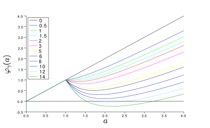
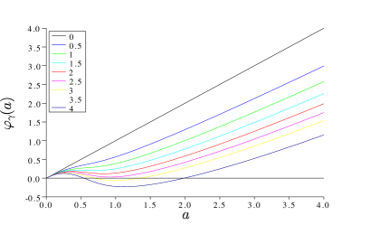
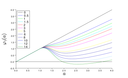
Figure 4. Plots of $a\mapsto\varphi_{\gamma}(a)$ for different values of $\gamma$, when $\lambda(v)=v^{2}$ (up left), $\lambda(v)=(v-1)_{+}^{2}$ (up right), $\lambda(v)=v^{4}$ (down left), $\lambda(v)=(v-1)_{+}^{4}$ (down right),

Let us comment on Figure 4. Recall that for $\gamma>0$ and $I>0$, each stationary solution to (8) corresponds to one solution $a$ to $\varphi_{\gamma}(a)=1$.

$\bullet$ If $\lambda(v)=v^{2}$, for any $\gamma>0$, the equation $\varphi_{\gamma}(a)=I$ (with $I>0$ fixed) seems to have exactly one solution, for all $I>0$.

$\bullet$ If $\lambda(v)=(v-1)_{+}^{2}$, $\lambda(v)=v^{4}$ or $\lambda(v)=(v-1)_{+}^{4}$, it seems that there are $0<\gamma_{1}<\gamma_{2}$ (e.g., $\gamma_{1}\simeq 1.5$ and $\gamma_{2}\simeq 12$ when $\lambda(v)=(v-1)_{+}^{4}$) such that

(a) if $\gamma\in(0,\gamma_{1})$, then for all $I>0$, $\varphi_{\gamma}(a)=I$ has exactly one solution,

(b) if $\gamma\in(\gamma_{1},\gamma_{2})$, then there are $0<J_{\gamma}<I_{\gamma}$ such that, if $I\in(0,J_{\gamma})$, $\varphi_{\gamma}(a)=I$ has exactly one solution, if $I\in(J_{\gamma},I_{\gamma})$, $\varphi_{\gamma}(a)=I$ has exactly three solutions and if $I>I_{\gamma}$, $\varphi_{\gamma}(a)=I$ has exactly one solution,

(c) if $\gamma\in(\gamma_{2},\infty)$, then there is $I_{\gamma}>0$ such that for all $I\in(0,I_{\gamma})$, $\varphi_{\gamma}(a)=I$ has exactly three solutions and if $I>I_{\gamma}$, $\varphi_{\gamma}(a)=I$ has exactly one solution (which is nontrivial).

8. Simulations

In all the simulations below, we have chosen the following values: the minimum potential is $v_{min}=0$, the length of the dendrites is $L=1$, the repartition density is $H(x)=2(1-x)$ on $[0,1]$, the front velocity is $\rho=1$ and the excitation parameter is $w=1$. Concerning the particle systems presented in Subsection 1.1, we consider a fully mean-field interaction, i.e. $p_{n}=1$ and $N=n$.

The code we use to simulate the soft particles system presented in Subsection 1.1 relies on a rejection method. The only difficulty concerns the treatment of the dendrites, that we need to incrementally update with new fronts. This is based on the recent algorithm of Yakupov and Buzdalov [39].

8.1. An isolated dendrite with i.i.d. impulses

We will observe in the next subsections a small temporal shift between the particle system and its mean-field limit. To explain this phenomenon, we consider a single dendrite with length $1$, on which two fronts start from each $X_{i}$ at time $T_{i}$ (for $i=1,\dots,n$), where the family $(T_{i},X_{i})_{i\geq 1}$ is i.i.d. with density ${\mathbbm{1}}_{\{t\in[0,1]\}}{\mathrm{d}}tH(x){\mathrm{d}}x$. The situation is thus very simple and, as seen in Proposition 2, $A_{t}(\sum_{i=1}^{n}\delta_{(T_{i},X_{i})})$ represents the number of fronts hitting the soma of the dendrite before time $t$. By Lemma 12, $Y^{n}_{t}=n^{-1/2}A_{t}(\sum_{i=1}^{n}\delta_{(T_{i},X_{i})})$ goes to $y_{t}=\Gamma_{t}(({\mathbbm{1}}_{\{s\in[0,1]\}})_{s\geq 0})$ as $n\to\infty$. By Remark 5, we have

$$y_{t}=\sqrt{2\rho H(0)}\int_{0}^{t}{\mathbbm{1}}_{\{s\in[0,1]\}}{\mathrm{d}}s=2\min(t,1).$$

We want to show that there is a systematic bias. So, we fix $K=10000$, we simulate $K$ i.i.d. copies $(Y^{i,n}_{t})_{t\in[0,2]}$ of the process $(Y^{n}_{t})_{t\in[0,2]}$, for different values of $n$, namely $n=10000$, $n=40000$ and $n=80000$. On Figure 5, we plot, as a function of time $t\in[0,2]$, the average values $K^{-1}\sum_{i=1}^{K}Y^{i,n}_{t}-y_{t}$. We observe a systematic negative bias, which remains important for large values of $n$. For example at time $1$ we have a bias around $-0.14$ (i.e. $7\%$) when $n=10000$ and $-0.08$ (i.e. $4\%$) when $n=80000$.

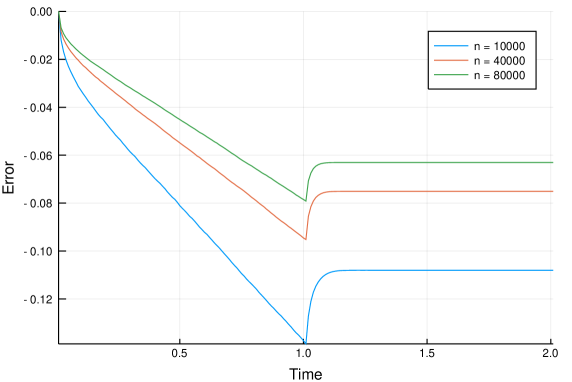
Figure 5. Isolated dendrite.

We see that a few late fronts arrive after time $1$ (while the limiting value stops increasing at time $1$) and this slightly makes decrease the bias.

8.2. The soft model without delay

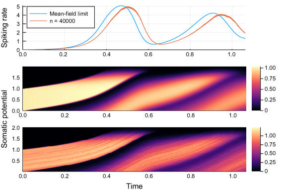
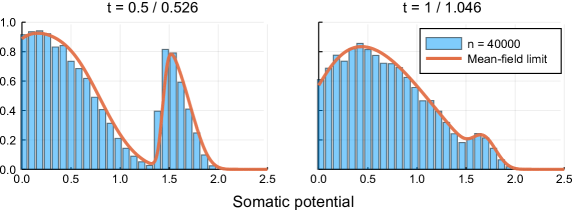
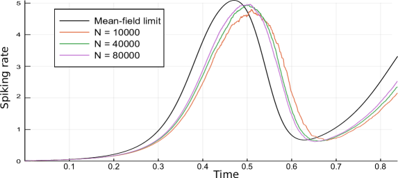
                 6.a                  6.b                  6.c

Figure 6. Soft model, $\theta\!=\!0$, $\lambda(v)\!=\!(v\!-\!0.2)_{+}^{8}$, $F(v)\!=\!1\!-\!0.1v$, $f_{0}(v)\!={\mathbbm{1}}_{[0,1]}(v)$.

Here we consider the soft model with the following parameters: the delay is $\theta=0$, the rate function is $\lambda(v)=\max(v-0.2,0)^{8}$, the drift function is $F(v)=1-0.1v$ and the initial distribution is $f_{0}(v)={\mathbbm{1}}_{\{v\in[0,1]\}}$. On Figure 6.a, we plot on the first picture the maps $t\mapsto n^{-1}\sum_{i=1}^{n}\lambda(V^{i,n}_{t})$, for the particle system (soft model) described in Subsection 1.1 with $n=40000$ particles, as well as $t\mapsto{\mathbb{E}}[\lambda(V_{t})]$, for $(V_{t})_{t\geq 0}$ the unique solution to the nonlinear SDE (3). We observe that the two curves are very similar, but there is a small temporal shift. This is related to what we explained in Subsection 8.1. The second picture represents $(g(t,v))_{t\geq 0,v\geq 0}$, where $g(t,\cdot)$ is the density of the law of $V_{t}$. The third picture represents $(g_{n}(t,v))_{t\geq 0,v\geq 0}$, still with $n=40000$, where $g_{n}(t,\cdot)$ is a smooth version of the empirical measure $n^{-1}\sum_{i=1}^{n}\delta_{V^{i,n}_{t}}$. Here again, the second and third pictures seem rather close, up to a small temporal shift. On Figure 6.b, the first picture represents $v\mapsto g(t,v)$ (with $t=0.5$) and $v\mapsto g_{n}(t,v)$ (with $t=0.526$). So, we took into account the temporal shift to make the histogram fit the continuous curve as well as possible. The second picture is similar, with $t=1$ and $t=1.046$. Finally, Figure 6.c contains a plot of $t\mapsto{\mathbb{E}}[\lambda(V_{t})]$ and of $t\mapsto n^{-1}\sum_{i=1}^{n}\lambda(V^{i,n}_{t})$ for different values of $n$. We see that the temporal shift decreases as $n$ increases, but the convergence seems to be rather slow.

Let us mention that $g(t,v)$ is computed here by solving numerically the PDE associated to the nonlinear SDE (3), using an Euler scheme relying on finite differences in $t$ and in $v$, with a regular grid. There is a source term at $v_{min}=0$ involving the integral $\int_{0}^{\infty}\lambda(v)g(t,v){\mathrm{d}}v$, that is incorporated in the spatial finite difference at the extremity $v=0$ of the space-grid. We take absolute values and normalize at each time step to ensure the positivity of the solution and that its total mass equals $1$. All the figures involving this scheme were compared to a simple interacting particle system (see the next subsection) and we found very similar results.

8.3. The soft model with delay

Here we proceed exactly as in Subsection 8.2, with the same parameters, except that the delay $\theta=0.4$. The results are presented in Figure 7. The unpleasant temporal shift is slightly smaller.

Let us mention that we use here a different scheme to approximate the law $g(t,\cdot)$ of $V_{t}$, based on a simple interacting particle system $(\bar{V}^{i,K}_{t})_{i=1,\dots,K,t\geq 0}$, with $K=10^{6}$ particles. Indeed, the scheme of the previous section was not stable with a nonzero delay. Roughly, each particle solves the same SDE as (3) (with i.i.d. initial conditions and driving Poisson measures), but with the nonlinear term $\int_{0}^{(t-\theta)\lor 0}(\gamma{\mathbb{E}}[\lambda(V_{s})])^{1/2}{\mathrm{d}}s$ replaced by its empirical version $\int_{0}^{(t-\theta)\lor 0}(\gamma K^{-1}\sum_{i=1}^{K}\lambda(\bar{V}_{s}^{i,K}))^{1/2}{\mathrm{d}}s$. Of course, we also have to proceed to a time discretization.

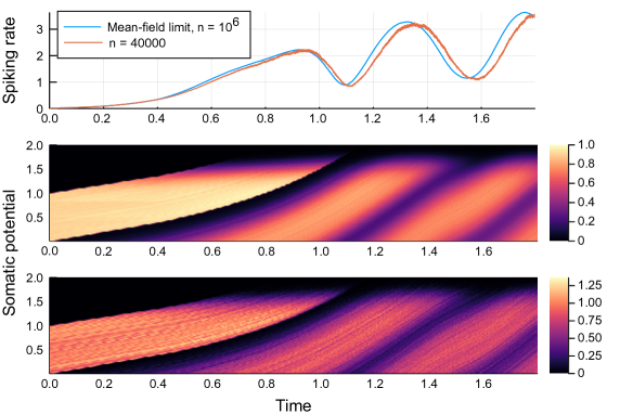
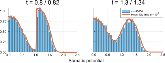
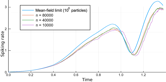
                 7.a                  7.b                  7.c

Figure 7. Soft model, $\theta\!=\!0.4$, $\lambda(v)\!=\!(v\!-\!0.2)_{+}^{8}$, $F(v)\!=\!1\!-\!0.1v$, $f_{0}(v)\!={\mathbbm{1}}_{[0,1]}(v)$.

8.4. The soft model with another rate function

Here again, we proceed exactly as in Subsection 8.2, with the same parameters (in particular $\theta=0$), except that the rate function $\lambda(v)=v^{8}$ does not satisfy our assumptions, since $\alpha=\inf\{v\geq v_{min}:\lambda(v)>0\}=v_{min}$ (recall that $v_{min}=0$). The results are presented in Figure 8 and are not less convincing than those of the previous subsections. It thus seems that our assumption that $\alpha>v_{min}$ is not necessary.

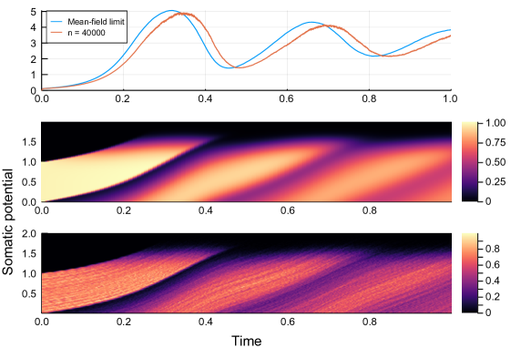
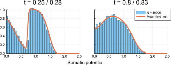
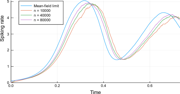
                 8.a                  8.b                  8.c

Figure 8. Soft model, $\theta\!=\!0$, $\lambda(v)\!=\!v^{8}$, $F(v)\!=\!1\!-\!0.1v$, $f_{0}(v)\!={\mathbbm{1}}_{[0,1]}(v)$.

8.5. The hard model

Concerning the hard model, we did not code the particle system described in Subsection 1.1. However, we would like to validate numerically the explicit formula of Theorem 11. We consider the following set of parameters: $F(v)=I=0.5$, $\theta=0$, $v_{min}=0$, $v_{max}=1.2$, and

$$f_{0}(v)=\Big{[}\frac{1}{2v_{max}}+\frac{\pi}{4v_{max}}\sin\frac{\pi v}{v_{max}}\Big{]}{\mathbbm{1}}_{[0,v_{max}]}(v).$$

We compute numerically $(\kappa_{t})_{t\geq 0}$ by solving the ODE $\kappa^{\prime}_{t}=G_{0}(v_{max}-It-\kappa_{t})$ (with $\kappa_{0}=0$), using an Euler scheme, until time $a>0$ such that $\kappa_{a}+Ia=v_{max}$ and by using that $\kappa^{\prime}$ is $a$-periodic, see the proof of Theorem 11. On Figure 9, we plot in red the curve $t\mapsto\kappa^{\prime}_{t}$. Recall that $\kappa^{\prime}_{t}$ represents the excitation rate, i.e. the increase of potential of the neurons, during $[t,t+{\mathrm{d}}t]$, due to excitation.

Next, the hard model can be seen as the soft model with the choice $\lambda(v)=\infty{\mathbbm{1}}_{\{v>v_{max}\}}$, that we approximate by $\lambda(v)=\max(v-0.2,0)^{300}$. We then the mean-field particle system introduced in Subsection 8.3) with $K=200000$ particles, to approximate numerically $t\mapsto{\mathbb{E}}[\lambda(V_{t})]$, $(V_{t})_{t\geq 0}$ being the solution to the nonlinear SDE (3). And we plot, in blue, the approximation of $t\mapsto 2\sqrt{{\mathbb{E}}[\lambda(V_{t})]}$, which also represents the excitation rate, since it is the derivative of $t\mapsto\Gamma_{t}(({\mathbb{E}}[\lambda(V_{s})])_{s\geq 0})=2\int_{0}^{t}\sqrt{{\mathbb{E}}[\lambda(V_{s})]}{\mathrm{d}}s$, see Remark 5 and recall that $H(0)=2$.

The two curves are close to each other and this is rather convincing concerning our explicit formula. However the precision is not high, which is not surprising due to the (numerical) singular behavior of $\lambda$ around $v=v_{max}$.

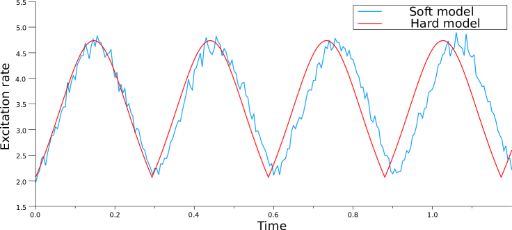
Figure 9. Soft and hard models with $\theta=0$, $F\equiv 0.5$, $v_{max}=1.2$, $\lambda(v)\!=\!(v\!-\!0.2)_{+}^{300}$ and $f_{0}(v)=[\frac{1}{2v_{max}}+\frac{\pi}{4v_{max}}\sin\frac{\pi v}{v_{max}}]{{\mathbbm{1}}_{[0,v_{max}]}(v)}.$

References

- [1] Aldous, D. and Diaconis, P. Hammersley’s interacting particle process and longest increasing subsequences. Probab. Theory Related Fields 103 (1995), 199–213.
- [2] Basdevant, A.L., Gerin, L., Gouéré, J.B. and Singh, A. From Hammersley’s lines to Hammersley’s trees. Probab. Theory Related Fields http://doi.org/10.1007/s00440-017-0772-2 (2017).
- [3] Bollobás, B. and Winkler, P. The longest chain among random points in Euclidean space. Proc. Amer. Math. Soc. 103 (1988), 347–353.
- [4] Bossy, M., Faugeras, O. and Talay, D. Clarification and complement to “Mean-field description and propagation of chaos in networks of Hodgkin-Huxley and FitzHugh-Nagumo neurons” J. Math. Neurosci. 5 (2015), 23 p.
- [5] Cáceres, M., Carrillo, J. and Perthame, B. Analysis of nonlinear noisy integrate & fire neuron models: blow-up and steady states. J. Math. Neurosci. 1 (2011), 33 p.
- [6] Calder, J., Esedoḡlu, S. and Hero, A.O. A Hamilton-Jacobi equation for the continuum limit of nondominated sorting. SIAM J. Math. Anal. 46 (2014), 603–638.
- [7] Carrillo, J., Perthame, B., Salort, D. and Smets, D. Qualitative properties of solutions for the noisy integrate and fire model in computational neuroscience. Nonlinearity 28 (2015), 3365–3388.
- [8] Cator, E. and Groeneboom, P. Hammersley’s process with sources and sinks. Ann. Probab. 33 (2005), 879–903.
- [9] Chevallier, J. Mean-field limit of generalized Hawkes processes. Stochastic Process. Appl. 127 (2017), 3870–3912.
- [10] Chevallier, J., Cáceres, M., Doumic, M. and Reynaud-Bouret, P. Microscopic approach of a time elapsed neural model. Math. Models Methods Appl. Sci. 25 (2015), 2669–2719.
- [11] Chevallier, J., Duarte, A., Löcherbach, E. and Ost, G. Mean field limits for nonlinear spatially extended Hawkes processes with exponential memory kernels. arXiv:1703.05031 (2017).
- [12] Delarue, F., Inglis, J., Rubenthaler, S. and Tanré, E. Global solvability of a networked integrate-and-fire model of McKean-Vlasov type. Ann. Appl. Probab. 25 (2015), 2096–2133.
- [13] Delarue, F., Inglis, J., Rubenthaler, S. and Tanré, E. Particle systems with a singular mean-field self-excitation. Application to neuronal networks. Stochastic Process. Appl. 125 (2015), 2451–2492.
- [14] De Masi, A., Galves, A., Löcherbach, E. and Presutti, E. Hydrodynamic limit for interacting neurons. J. Stat. Phys. 158 (2015), 866–902.
- [15] Deuschel, J.D. and Zeitouni, O. Limiting curves for i.i.d. records. Ann. Probab. 23 (1995), 852–878.
- [16] Ditlevsen, S. and Löcherbach, E. Multi-class oscillating systems of interacting neurons. Stochastic Process. Appl. 127, (2017), 1840–1869.
- [17] Fournier, N. and Löcherbach, E. On a toy model of interacting neurons. Ann. Inst. Henri Poincaré Probab. Stat. 52 (2016), 1844–1876.
- [18] Górski T., Veltz R., Galtier M., Fragnaud H., Telenczuk B. and Destexhe A. Dendritic sodium spikes endow neurons with inverse firing rate response to correlated synaptic activity. J. Comput. Neurosci. 45, (2018), 223–234.
- [19] Hammersley, J.M. A few seedlings of research. Proceedings of the Sixth Berkeley Symposium on Mathematical Statistics and Probability (Univ. California, Berkeley, Calif., 1970/1971), Vol. I: Theory of statistics, Univ. California Press, Berkeley, Calif., 345–394, 1972.
- [20] Hodgkin, A. L. and Huxley, A. F. A quantitative description of membrane current and its application to conduction and excitation in nerve The Journal of Physiology, 117 (1952), 500–544.
- [21] Inglis, J. and Talay, D. Mean-field limit of a stochastic particle system smoothly interacting through threshold hitting-times and applications to neural networks with dendritic component. SIAM J. Math. Anal. 47 (2015), 3884–3916.
- [22] Kac, M. Foundations of kinetic theory. In Proceedings of the Third Berkeley Symposium on Mathematical Statistics and Probability, 1954-1955, vol. III (Berkeley and Los Angeles, 1956), University of California Press, pp. 171–197.
- [23] Kandel, E.R., Principles of neural science. 5th ed. New York: McGraw-Hill, 2013.
- [24] Koch, C. Biophysics of Computation: Information Processing in Single Neurons. Oxford Univ. Press paperback. Computational Neuroscience. New York: Oxford Univ. Press, 2004.
- [25] Logan, B.F. and Shepp, L.A. A variational problem for random Young tableaux. Advances in Math. 26 (1977), 206–222.
- [26] Luçon, E. Quenched limits and fluctuations of the empirical measure for plane rotators in random media Electron. J. Probab. 16 (2011), 792–829.
- [27] Luçon, E. and Stannat, W. Mean field limit for disordered diffusions with singular interactions. Ann. Appl. Probab. 24 (2014), 1946–1993.
- [28] Luçon, E. and Stannat, W. Transition from Gaussian to non-Gaussian fluctuations for mean-field diffusions in spatial interaction. Ann. Appl. Probab. 26 (2016), 3840–3909.
- [29] McKean, H. P. Propagation of chaos for a class of non-linear parabolic equations. Lecture series in differential equations 7 (1967), Catholic University, Washington, 41–57.
- [30] Méléard, S. Asymptotic behaviour of some interacting particle systems; McKean-Vlasov and Boltzmann models. Probabilistic models for nonlinear partial differential equations, 42–95, Lecture Notes in Math., 1627, Fond. CIME, Springer, Berlin, 1996.
- [31] Ostojic, S., Brunel, N. and Hakim, V., Synchronization properties of networks of electrically coupled neurons in the presence of noise and heterogeneities. J. Comput. Neurosci. 26 (2009), 369–392.
- [32] Pakdaman, K., Thieullen, M. and Wainrib, G. Fluid limit theorems for stochastic hybrid systems with application to neuron models. Adv. in Appl. Probab. 42 (2010), 761–794.
- [33] Renart, A., Brunel, N. and Wang, X.-J. Mean-field theory of irregularly spiking neuronal populations and working memory in recurrent cortical networks. Computational Neuroscience: A comprehensive approach., Chapman & Hall/CRC Mathematical Biology and Medicine Series, (2004), 431–490.
- [34] Riedler, M., Thieullen, M. and Wainrib, G., Limit theorems for infinite-dimensional piecewise deterministic Markov processes. Applications to stochastic excitable membrane models. Electron. J. Probab. 17 (2012), 48p.
- [35] Stuart, G., Spruston N. and Häusser M., Dendrites. 3rd ed. Oxford; New York: Oxford University Press, 2015.
- [36] Sznitman, A.-S. Topics in propagation of chaos. In École d’Été de Probabilités de Saint-Flour XIX—1989, vol. 1464 of Lecture Notes in Math. Springer, Berlin, 1991, 165–251.
- [37] Ulam, S.M. Monte Carlo calculations in problems of mathematical physics. Modern mathematics for the engineer: Second series, McGraw-Hill, New York, 261–281, 1961.
- [38] Versik, A.M. and Kerov, S.V. Asymptotic behavior of the Plancherel measure of the symmetric group and the limit form of Young tableaux. Dokl. Akad. Nauk SSSR 233 (1977), 1024–1027.
- [39] Yakupov, I. and Buzdalov, M. Incremental non-dominated sorting with O(N) insertion for the two-dimensional case. In IEEE Congress on Evolutionary Computation (CEC) 1853–1860, 2015.