Randomized Block Cubic Newton Method

Appendix

Abstract

We study the problem of minimizing the sum of three convex functions—a differentiable, twice-differentiable and a non-smooth term—in a high dimensional setting. To this effect we propose and analyze a randomized block cubic Newton (RBCN) method, which in each iteration builds a model of the objective function formed as the sum of the natural models of its three components: a linear model with a quadratic regularizer for the differentiable term, a quadratic model with a cubic regularizer for the twice differentiable term, and perfect (proximal) model for the nonsmooth term. Our method in each iteration minimizes the model over a random subset of blocks of the search variable. RBCN is the first algorithm with these properties, generalizing several existing methods, matching the best known bounds in all special cases. We establish ${\cal O}(1/\epsilon)$, ${\cal O}(1/\sqrt{\epsilon})$ and ${\cal O}(\log(1/\epsilon))$ rates under different assumptions on the component functions. Lastly, we show numerically that our method outperforms the state of the art on a variety of machine learning problems, including cubically regularized least-squares, logistic regression with constraints, and Poisson regression.

1 Introduction

In this paper we develop an efficient randomized algorithm for solving an optimization problem of the form

$$\min_{x\in Q}F(x)\stackrel{{\scriptstyle\mathrm{def}}}{{=}}g(x)+\phi(x)+\psi(x),$$ (1)

where $Q\subseteq\mathbb{R}^{N}$ is a closed convex set, and $g,\phi$ and $\psi$ are convex functions with different smoothness and structural properties. Our aim is to capitalize on these different properties in the design of our algorithm. We assume that $g$ has Lipschitz gradient, $\phi$ has Lipschitz Hessian, while $\psi$ is allowed to be nonsmooth, albeit “simple”.

1.1 Block Structure

Moreover, we assume that the $N$ coordinates of $x$ are partitioned into $n$ blocks of sizes $N_{1},\dots,N_{n}$, with $\sum_{i}N_{i}=N$, and then write $x=(x_{(1)},\dots,x_{(n)})$, where $x_{(i)}\in\mathbb{R}^{N_{i}}$. This block structure is typically dictated by the particular application considered. Once the block structure is fixed, we further assume that $\phi$ and $\psi$ are block separable. That is, $\phi(x)=\sum_{i=1}^{n}\phi_{i}(x_{(i)})$ and $\psi(x)=\sum_{i=1}^{n}\psi_{i}(x_{(i)})$, where $\phi_{i}$ are twice differentiable with Lipschitz Hessians, and $\psi_{i}$ are closed convex (and possibly nonsmooth) functions.

Revealing this block structure, problem (1) takes the form

$$\min_{x\in Q}F(x)\stackrel{{\scriptstyle\mathrm{def}}}{{=}}g(x)+\sum_{i=1}^{n}\phi_{i}(x_{(i)})+\sum_{i=1}^{n}\psi_{i}(x_{(i)}).$$ (2)

We are specifically interested in the case when $n$ is big, in which case it make sense to update a small number of the block in each iteration only.

1.2 Related Work

There has been a substantial and growing volume of research related to second-order and block-coordinate optimization. In this part we briefly mention some of the papers most relevant to the present work.

A major leap in second-order optimization theory was made since the cubic Newton method was proposed by Griewank (1981) and independently rediscovered by Nesterov & Polyak (2006), who also provided global complexity guarantees.

Cubic regularization was equipped with acceleration by Nesterov (2008), adaptive stepsizes by (Cartis et al., 2011a, b) and extended to a universal framework by Grapiglia & Nesterov (2017). The universal schemes can automatically adjust to the implicit smoothness level of the objective. Cubically regularized second-order schemes for solving systems of nonlinear equations were developed by Nesterov (2007) and randomized variants for stochastic optimization were considered by Tripuraneni et al. (2017); Ghadimi et al. (2017); Kohler & Lucchi (2017); Cartis & Scheinberg (2018).

Despite their attractive global iteration complexity guarantees, the weakness of second-order methods in general, and cubic Newton in particular, is their high computational cost per iteration. This issue remains the subject of active research. For successful theoretical results related to the approximation of the cubic step we refer to (Agarwal et al., 2016) and (Carmon & Duchi, 2016).

At the same time, there are many successful attempts to use block coordinate randomization to accelerate first-order (Tseng & Yun, 2009; Richtárik & Takáč, 2014, 2016) and second-order (Qu et al., 2016; Mutnỳ & Richtárik, 2018) methods.

In this work we are addressing the issue of combining block-coordinate randomization with cubic regularization, to get a second-order method with proven global complexity guarantees and with a low cost per iteration.

A powerful advance in convex optimization theory was the advent of composite or proximal first-order methods (see (Nesterov, 2013) as a modern reference). This technique has become available as an algorithmic tool in block coordinate setting as well (Richtárik & Takáč, 2014; Qu et al., 2016). Our aim in this work is the development of a composite cubically regularized second-order method.

1.3 Contributions

We propose a new randomized second-order proximal algorithm for solving convex optimization problems of the form (2). Our method, Randomized Block Cubic Newton (RBCN) (see Algorithm 1) treats the three functions appearing in (1) differently, according to their nature.

Our method is a randomized block method because in each iteration we update a random subset of the $n$ blocks only. This facilitates faster convergence, and is suited to problems where $n$ is very large. Our method is proximal because we keep the functions $\psi_{i}$ in our model, which is minimized in each iteration, without any approximation. Our method is a cubic Newton method because we approximate each $\phi_{i}$ using a cubically-regularized second order model.

We are not aware of any method that can solve (2) via using the most appropriate models of the three functions (quadratic with a constant Hessian for $g$, cubically regularized quadratic for $\phi$ and no model for $\psi$), not even in the case $n=1$.

Our approach generalizes several existing results:

• In the case when $n=1$, $g=0$ and $\psi=0$, RBCN reduces to the cubically-regularized Newton method of Nesterov & Polyak (2006). Even when $n=1$, RBCN can be seen as an extension of this method to composite optimization. For $n>1$, RBCN provides an extension of the algorithm in Nesterov & Polyak (2006) to the randomized block coordinate setting, popular for high-dimensional problems.

• In the special case when $\phi=0$ and $N_{i}=1$ for all $i$, RBCN specializes to the stochastic Newton (SN) method of Qu et al. (2016). Applied to the empirical risk minimization problem (see Section 7), our method has a dual interpretation (see Algorithm 2). In this case, our method reduces to the stochastic dual Newton ascent method (SDNA) also described in (Qu et al., 2016). Hence, RBCN can be seen as an extension of SN and SDNA to blocks of arbitrary sizes, and to the inclusion of the twice differentiable term $\phi$.

• In the case when $\phi=0$ and the simplest over approximation of $g$ is assumed: $0\preceq\nabla^{2}g(x)\preceq LI$, the composite block coordinate gradient method Tseng & Yun (2009) can be applied to solve (1). Our method extends this in two directions: we add twice-differentiable terms $\phi$, and use a tighter model for $g$, using all global curvature information (if available).

We prove high probability global convergence guarantees under several regimes, summarized next:

• Under no additional assumptions on $g$, $\phi$ and $\psi$ beyond convexity (and either boundedness of $Q$, or boundedness of the level sets of $F$ on $Q$), we prove the rate

  $${\cal O}\left(\frac{n}{\tau\epsilon}\right),$$

  where $\tau$ is the mini-batch size (see Theorem 1).

• Under certain conditions combining the properties of $g$ with the way the random blocks are sampled, formalized by the assumption $\beta>0$ (see (12) for the definition of $\beta$), we obtain the rate

  $${\cal O}\left(\frac{n}{\tau\max\{1,\beta\}\sqrt{\epsilon}}\right)$$

  (see Theorem 2). In the special case when $n=1$, we necessarily have $\tau=1$ and $\beta=\mu/L$ (reciprocal of the condition number of $g$) we get the rate ${\cal O}(\tfrac{L}{\mu\sqrt{\epsilon}})$. If $g$ is quadratic and $\tau=n$, then $\beta=1$ and the resulting complexity ${\cal O}(\tfrac{1}{\sqrt{\epsilon}})$ recovers the rate of cubic Newton established by Nesterov & Polyak (2006).

• Finally, if $g$ is strongly convex, the above result can be improved (see Theorem 3) to

  $${\cal O}\left(\frac{n}{\tau\max\{1,\beta\}}\log\frac{1}{\epsilon}\right).$$

1.4 Contents

The rest of the paper is organized as follows. In Section 2 we introduce the notation and elementary identities needed to efficiently handle the block structure of our model. In Section 3 we make the various smoothness and convexity assumptions on $g$ and $\phi_{i}$ formal. Section 4 is devoted to the description of the block sampling process used in our method, along with some useful identities. In Section 5 we describe formally our randomized block cubic Newton (RBCN) method. Section 6 is devoted to the statement and description of our main convergence results, summarized in the introduction. Missing proofs are provided in the supplementary material. In Section 7 we show how to apply our method to the empirical risk minimization problem. Applying RBCN to its dual leads to Algorithm 2. Finally, our numerical experiments on synthetic and real datasets are described in Section 8.

2 Block Structure

To model a block structure, we decompose the space $\mathbb{R}^{N}$ into $n$ subspaces in the following standard way. Let ${\bf U}\in\mathbb{R}^{N\times N}$ be a column permutation of the $N\times N$ identity matrix ${\bf I}$ and let a decomposition ${\bf U}=[{\bf U}_{1},{\bf U}_{2},\dots,{\bf U}_{n}]$ be given, where ${\bf U}_{i}\in\mathbb{R}^{N\times N_{i}}$ are $n$ submatrices, $N=\sum_{i=1}^{n}N_{i}$. Subsequently, any vector $x\in\mathbb{R}^{N}$ can be uniquely represented as $x=\sum_{i=1}^{n}{\bf U}_{i}x_{(i)}$, where $x_{(i)}\stackrel{{\scriptstyle\mathrm{def}}}{{=}}{\bf U}_{i}^{T}x\in\mathbb{R}^{N_{i}}$.

In what follows we will use the standard Euclidean inner product: $\langle x,y\rangle\stackrel{{\scriptstyle\mathrm{def}}}{{=}}\sum_{i}x_{i}y_{i}$, Euclidean norm of a vector: $\|x\|\stackrel{{\scriptstyle\mathrm{def}}}{{=}}\sqrt{\langle x,x\rangle}$ and induced spectral norm of a matrix: $\|{\bf A}\|\stackrel{{\scriptstyle\mathrm{def}}}{{=}}\max_{\|x\|=1}\|{\bf A}x\|$. Using block decomposition, for two vectors $x,y\in\mathbb{R}^{N}$ we have:

$$\langle x,y\rangle=\biggl{\langle}\sum_{i=1}^{n}{\bf U}_{i}x_{(i)},\sum_{j=1}^{n}{\bf U}_{j}y_{(j)}\biggl{\rangle}=\sum_{i=1}^{n}\langle x_{(i)},y_{(i)}\rangle.$$

For a given nonempty subset $S$ of $[n]\stackrel{{\scriptstyle\mathrm{def}}}{{=}}\{1,\dots,n\}$ and for any vector $x\in\mathbb{R}^{N}$ we denote by $x_{[S]}\in\mathbb{R}^{N}$ the vector obtained from $x$ by retaining only blocks $x_{(i)}$ for which $i\in S$ and zeroing all other:

$$x_{[S]}\stackrel{{\scriptstyle\mathrm{def}}}{{=}}\sum_{i\in S}{\bf U}_{i}x_{(i)}=\sum_{i\in S}{\bf U}_{i}{\bf U}_{i}^{T}x.$$

Furthermore, for any matrix ${\bf A}\in\mathbb{R}^{N\times N}$ we write ${\bf A}_{[S]}\in\mathbb{R}^{N\times N}$ for the matrix obtained from ${\bf A}$ by retaining only elements whose indices are both in some coordinate blocks from $S$, formally:

$${\bf A}_{[S]}\stackrel{{\scriptstyle\mathrm{def}}}{{=}}\Biggl{(}\sum_{i\in S}{\bf U}_{i}{\bf U}_{i}^{T}\Biggr{)}{\bf A}\Biggl{(}\sum_{i\in S}{\bf U}_{i}{\bf U}_{i}^{T}\Biggr{)}.$$

Note that these definitions imply that

$$\langle{\bf A}_{[S]}x,y\rangle=\langle{\bf A}x_{[S]},y_{[S]}\rangle,\quad x,y\in\mathbb{R}^{N}.$$

Next, we define the block-diagonal operator, which, up to permutation of coordinates, retains diagonal blocks and nullifies the off-diagonal blocks:

$$\operatorname{blockdiag}({\bf A})\stackrel{{\scriptstyle\mathrm{def}}}{{=}}\sum_{i=1}^{n}{\bf U}_{i}{\bf U}_{i}^{T}{\bf A}{\bf U}_{i}{\bf U}_{i}^{T}=\sum_{i=1}^{n}{\bf A}_{[\{i\}]}.$$

Finally, denote $\mathbb{R}^{N}_{[S]}\stackrel{{\scriptstyle\mathrm{def}}}{{=}}\bigl{\{}x_{[S]}\,|\,x\in\mathbb{R}^{N}\bigr{\}}$. This is a linear subspace of $\mathbb{R}^{N}$ composed of vectors which are zero in blocks $i\notin S$.

3 Assumptions

In this section we formulate our main assumptions about differentiable components of (2) and provide some examples to illustrate the concepts.

We assume that $g:\mathbb{R}^{N}\to\mathbb{R}$ is a differentiable function and all $\phi_{i}:\mathbb{R}^{N_{i}}\to\mathbb{R},\;i\in[n]$ are twice differentiable. Thus, at any point $x\in\mathbb{R}^{N}$ we should be able to compute all the gradients $\{\nabla g(x),\nabla\phi_{1}(x_{(1)}),\dots,\nabla\phi_{n}(x_{(n)})\}$ and the Hessians $\{\nabla^{2}\phi_{1}(x_{(1)}),\dots,\nabla^{2}\phi_{n}(x_{(n)})\}$, or at least their actions on arbitrary vector $h$ of appropriate dimension.

Next, we formalize our assumptions about convexity and level of smoothness. Speaking informally, $g$ is similar to a quadratic, and functions $\phi_{i}$ are arbitrary twice-differentiable and smooth.

Assumption 1 (Convexity)

There is a positive semidefinite matrix ${\bf G}\succeq 0$ such that for all $x,h\in\mathbb{R}^{N}$:

$$g(x+h) \geq g(x)+\langle\nabla g(x),h\rangle+\frac{1}{2}\langle{\bf G}h,h\rangle,$$ (3)

$$\phi_{i}(x_{(i)}+h_{(i)}) \geq\phi_{i}(x_{(i)})+\langle\nabla\phi_{i}(x_{(i)}),h_{(i)}\rangle,\quad i\in[n].$$

In the special case when ${\bf G}=0$, (3) postulates convexity. For positive definite ${\bf G}$, the objective will be strongly convex with the strong convexity parameter $\mu\stackrel{{\scriptstyle\mathrm{def}}}{{=}}\lambda_{\min}({\bf G})>0$.

Note that for all $\phi_{i}$ we only require convexity. However, if we happen to know that any $\phi_{i}$ is strongly convex ($\lambda_{\min}(\nabla^{2}\phi_{i}(y))\geq\mu_{i}>0$ for all $y\in\mathbb{R}^{N_{i}}$), we can move this strong convexity to $g$ by subtracting $\frac{\mu_{i}}{2}\|x_{(i)}\|^{2}$ from $\phi_{i}$ and adding it to $g$. This extra knowledge may in some particular cases improve convergence guarantees for our algorithm, but does not change the actual computations.

Assumption 2 (Smoothness of $\boldsymbol{g}$)

There is a positive semidefinite matrix ${\bf A}\succeq 0$ such that for all $x,h\in\mathbb{R}^{N}$:

$$g(x+h)\leq g(x)+\langle\nabla g(x),h\rangle+\frac{1}{2}\langle{\bf A}h,h\rangle.$$ (4)

The main example of $g$ is a quadratic function $g(x)=\frac{1}{2}\langle{\bf M}x,x\rangle$ with a symmetric positive semidefinite ${\bf M}\in\mathbb{R}^{N\times N}$ for which both (3) and (4) hold with ${\bf G}={\bf A}={\bf M}$.

Of course, any convex $g$ with Lipschitz-continuous gradient with a constant $L\geq 0$ satisfies (3) and (4) with ${\bf G}=0$ and ${\bf A}=L{\bf I}$ (Nesterov, 2004).

Assumption 3 (Smoothness of $\boldsymbol{\phi_{i}}$)

For every $i\in[n]$ there is a nonnegative constant $\mathcal{H}_{i}\geq 0$ such that the Hessian of $\phi_{i}$ is Lipschitz-continuous:

$$\|\nabla^{2}\phi_{i}(x+h)-\nabla^{2}\phi_{i}(x)\|\leq\mathcal{H}_{i}\|h\|,$$ (5)

for all $x,h\in\mathbb{R}^{N_{i}}$.

Examples of functions which satisfy (5) with a known Lipschitz constant of Hessian $\mathcal{H}$ are quadratic: $\phi(t)=\|Ct-t_{0}\|^{2}$ ($\mathcal{H}=0$ for all the parameters), cubed norm: $\phi(t)=(1/3)\|t-t_{0}\|^{3}$ ($\mathcal{H}=2$, see Lemma 5 in (Nesterov, 2008)), logistic regression loss: $\phi(t)=\log(1+\exp(t))$ ($\mathcal{H}=1/(6\sqrt{3})$, see Proposition 1 in the supplementary material).

For a fixed set of indices $S\subset[n]$ denote

$$\phi_{S}(x)\stackrel{{\scriptstyle\mathrm{def}}}{{=}}\sum_{i\in S}\phi_{i}(x_{(i)}),\quad x\in\mathbb{R}^{N}.$$

Then we have:

$$\langle\nabla\phi_{S}(x),h\rangle =\sum_{i\in S}\langle\nabla\phi_{i}(x_{(i)}),h_{(i)}\rangle,\quad x,h\in\mathbb{R}^{N},$$

$$\langle\nabla^{2}\phi_{S}(x)h,h\rangle =\sum_{i\in S}\langle\nabla^{2}\phi_{i}(x_{(i)})h_{(i)},h_{(i)}\rangle,\quad x,h\in\mathbb{R}^{N}.$$

Lemma 1

If Assumption 3 holds, then for all $x,h\in\mathbb{R}^{N}$ we have the following second-order approximation bound:

$$\Bigl{|}\phi_{S}(x+h)-\phi_{S}(x) -\langle\nabla\phi_{S}(x),h\rangle-\frac{1}{2}\langle\nabla^{2}\phi_{S}(x)h,h\rangle\Bigr{|}$$

$$\leq \quad\max_{i\in S}\{\mathcal{H}_{i}\}\cdot\|h_{[S]}\|^{3}.$$ (6)

From now on we denote $\displaystyle\mathcal{H}_{\!F}\stackrel{{\scriptstyle\mathrm{def}}}{{=}}\max\{\mathcal{H}_{1},\mathcal{H}_{2},\dots,\mathcal{H}_{n}\}$.

4 Sampling of Blocks

In this section we summarize some basic properties of sampling $\hat{S}$, which is a random set-valued mapping with values being subsets of $[n]$. For a fixed block-decomposition, with each sampling $\hat{S}$ we associate the probability matrix ${\bf P}\in\mathbb{R}^{N\times N}$ as follows: an element of ${\bf P}$ is the probability of choosing a pair of blocks which contains indices of this element. Denoting by ${\bf E}\in\mathbb{R}^{N\times N}$ the matrix of all ones, we have ${\bf P}=\mathbb{E}\bigl{[}{\bf E}_{[\hat{S}]}\bigr{]}$. Wel restrict our analysis to uniform samplings, defined next.

Assumption 4 (Uniform sampling)

Sampling $\hat{S}$ is uniform, i.e., $\mathbb{P}(i\in\hat{S})=\mathbb{P}(j\in\hat{S})\stackrel{{\scriptstyle\mathrm{def}}}{{=}}p$, for all $i,j\in[n]$.

The above assumpotion means that the diagonal of ${\bf P}$ is constant: ${\bf P}_{ii}=p$ for all $i\in[N]$. It is easy to see that (Corollary 3.1 in (Qu & Richtárik, 2016)):

$$\mathbb{E}\bigl{[}{\bf A}_{[\hat{S}]}\bigr{]}={\bf A}\circ{\bf P},$$ (7)

where $\circ$ denotes the Hadamard product.

Denote $\tau\stackrel{{\scriptstyle\mathrm{def}}}{{=}}\mathbb{E}[|\hat{S}|]=np$ (expected minibatch size). The special uniform sampling defined by picking from all subsets of size $\tau$ uniformly at random is called $\tau$-nice sampling. If $\hat{S}$ is $\tau$-nice, then (see Lemma 4.3 in (Qu & Richtárik, 2016))

$${\bf P}=\frac{\tau}{n}\left((1-\gamma)\operatorname{blockdiag}({\bf E})+\gamma{\bf E}\right),$$ (8)

where $\gamma=(\tau-1)/(n-1)$.

In particular, the above results in the following:

Lemma 2

For the $\tau$-nice sampling $\hat{S}$, we have

$$\mathbb{E}[{\bf A}_{[\hat{S}]}]=\frac{\tau}{n}\left(1-\frac{\tau-1}{n-1}\right)\operatorname{blockdiag}({\bf A})+\frac{\tau(\tau-1)}{n(n-1)}{\bf A}.$$

Proof: Combine (7) and (8).  

5 Algorithm

Due to the problem structure (2) and utilizing the smoothness of the components (see (4) and (5)), for a fixed subset of indices $S\subset[n]$ it is natural to consider the following model of our objective $F$ around a point $x\in\mathbb{R}^{N}$:

$$M_{H,S}(x;y)\stackrel{{\scriptstyle\mathrm{def}}}{{=}}F(x)+\langle(\nabla g(x))_{[S]},y\rangle+\frac{1}{2}\langle{\bf A}_{[S]}y,y\rangle+$$

$$+\langle(\nabla\phi(x))_{[S]},y\rangle+\frac{1}{2}\langle(\nabla^{2}\phi(x))_{[S]}y,y\rangle+\frac{H}{6}\|y_{[S]}\|^{3}+$$

$$+\sum_{i\in S}\Bigl{(}\psi_{i}(x_{(i)}+y_{(i)})-\psi_{i}(x_{(i)})\Bigr{)}.$$ (9)

The above model arises as a combination of a first-order model for $g$ with global curvature information provided by matrix ${\bf A}$, second-order model with cubic regularization (following (Nesterov & Polyak, 2006)) for $\phi$, and perfect model for the non-differentiable terms $\psi_{i}$ (i.e., we keep these terms as they are).

Combining (4) and (1), and for large enough $H$ ($H\geq\max_{i\in S}\mathcal{H}_{i}$ is sufficient), we get the global upper bound

$$F(x+y)\leq M_{H,S}(x;y),\quad x\in\mathbb{R}^{N},\;y\in\mathbb{R}_{[S]}^{N}.$$

Moreover, the value of all summands in $M_{H,S}(x;y)$ depends on the subset of blocks $\{y_{(i)}|i\in S\}$ only, and therefore

$$T_{H,S}(x)\stackrel{{\scriptstyle\mathrm{def}}}{{=}}\mathop{\rm argmin}_{\begin{subarray}{c}y\in\mathbb{R}_{[S]}^{N}\\[2.0pt] \text{subject to}\;x+y\in Q\end{subarray}}M_{H,S}(x;y)$$ (10)

can be computed efficiently for small $|S|$ and as long as $Q$ is simple (for example, affine). Denote the minimum of the cubic model by $M^{*}_{H,S}(x)\stackrel{{\scriptstyle\mathrm{def}}}{{=}}M_{H,S}(x;T_{H,S}(x))$. The RBCN method performs the update $x\leftarrow x+T_{H,S}(x)$, and is formalized as Algorithm 1.

Algorithm 1 RBCN: Randomized Block Cubic Newton

1:  Parameters: sampling distribution $\hat{S}$

2:  Initialization: choose initial point $x^{0}\in Q$

3:  for $k=0,1,2,\dots$ do

4:     Sample $S_{k}\sim\hat{S}$

5:     Find $H_{k}\in(0,\,2\mathcal{H}_{\!F}]$ such that $\qquad F(x^{k}+T_{H_{k},S_{k}}(x^{k}))\leq M^{*}_{H_{k},S_{k}}(x^{k})$

6:     Make the step $x^{k+1}\stackrel{{\scriptstyle\mathrm{def}}}{{=}}x^{k}+T_{H_{k},S_{k}}(x^{k})$

7:  end for

6 Convergence Results

In this section we establish several convergence rates for Algorithm 1 under various structural assumptions: for the general class of convex problems, and for the more specific strongly convex case. We will focus on the family of uniform samplings only, but generalizations to other sampling distributions are also possible.

6.1 Convex Loss

We start from the general situation where the term $g(x)$ and all the $\phi_{i}(x_{(i)})$ and $\psi_{i}(x_{(i)}),i\in[n]$ are convex, but not necessary strongly convex.

Denote by $D$ the maximum distance from an optimum point $x^{*}$ to the initial level set:

$$D\stackrel{{\scriptstyle\mathrm{def}}}{{=}}\sup\Bigl{\{}\|x-x^{*}\|\;\big{|}\;x\in Q,\,F(x)\leq F(x^{0})\Bigr{\}}.$$

Theorem 1

Let Assumptions 1, 2, 3, 4 hold. Let solution $x^{*}\in Q$ of problem (1) exist, and assume the level sets are bounded: $D<+\infty$. Choose required accuracy $\varepsilon>0$ and confidence level $\rho\in(0,1)$. Then after

$$K\geq\frac{2}{\varepsilon}\frac{n}{\tau}\biggl{(}1+\log\frac{1}{\rho}\biggr{)}\max\Bigl{\{}LD^{2}+\mathcal{H}_{\!F}D^{3},\,F(x^{0})-F^{*}\Bigr{\}}$$ (11)

iterations of Algorithm 1, where $L\stackrel{{\scriptstyle\mathrm{def}}}{{=}}\lambda_{\max}({\bf A})$, we have

$$\mathbb{P}\Bigl{(}F(x^{K})-F^{*}\leq\varepsilon\Bigr{)}\;\geq\;1-\rho.$$

Given theoretical result provides global sublinear rate of convergence, with iteration complexity of the order $O\bigl{(}1/\varepsilon\bigr{)}$.

Note that for a case $\phi(x)\equiv 0$ we can put $\mathcal{H}_{\!F}=0$, and Theorem 1 in this situation restates well-known result about convergence of composite gradient-type block-coordinate methods (see, for example, (Richtárik & Takáč, 2014)).

6.2 Strongly Convex Loss

Here we study the case when the matrix ${\bf G}$ from the convexity assumption (3) is strictly positive definite: ${\bf G}\succ 0$, which means that the objective $F$ is strongly convex with a constant $\mu~{}\stackrel{{\scriptstyle\mathrm{def}}}{{=}}~{}\lambda_{\min}({\bf G})~{}>~{}0$.

Denote by $\beta$ a condition number for the function $g$ and sampling distribution $\hat{S}$: the maximum nonnegative real number such that

$$\beta\cdot\mathbb{E}_{S\sim\hat{S}}\bigl{[}{\bf A}_{[S]}\bigr{]}\;\preceq\;\frac{\tau}{n}{\bf G}.$$ (12)

If (12) holds for all nonnegative $\beta$ we put by definition $\beta\equiv+\infty$.

A simple lower bound exists: $\beta\geq\frac{\mu}{L}>0$, where $L=\lambda_{\max}({\bf A})$, as in Theorem 1. However, because (12) depends not only on $g$, but also on sampling distribution $\hat{S}$, it is possible that $\beta>0$ even if $\mu=0$ (for example, $\beta=1$ if $\mathbb{P}(S=[n])=1$ and ${\bf A}={\bf G}\not=0$).

The following theorems describe global iteration complexity guarantees of the order $O\bigl{(}1/\sqrt{\varepsilon}\bigr{)}$ and $O\bigl{(}\log(1/\varepsilon)\bigr{)}$ for Algorithm 1 in the cases $\beta>0$ and $\mu>0$ correspondingly, which is an improvement of general $O\bigl{(}1/\varepsilon\bigr{)}$.

Theorem 2

Let Assumptions 1, 2, 3, 4 hold. Let solution $x^{*}\in Q$ of problem (1) exist, let level sets be bounded: $D<+\infty$, and assume that $\beta$, which is defined by (12), is greater than zero. Choose required accuracy $\varepsilon>0$ and confidence level $\rho\in(0,1)$. Then after

$$K\geq\frac{2}{\sqrt{\varepsilon}}\frac{n}{\tau}\frac{1}{\sigma}\biggl{(}2+\log\frac{1}{\rho}\biggr{)}\sqrt{\max\Bigl{\{}\mathcal{H}_{\!F}D^{3},\,F(x^{0})-F^{*}\Bigr{\}}}$$ (13)

iterations of Algorithm 1, where $\sigma\stackrel{{\scriptstyle\mathrm{def}}}{{=}}\min\{\beta,1\}>0$, we have

$$\mathbb{P}\Bigl{(}F(x^{K})-F^{*}\leq\varepsilon\Bigr{)}\;\geq\;1-\rho.$$

Theorem 3

Let Assumptions 1, 2, 3, 4 hold. Let solution $x^{*}\in Q$ of problem (1) exist, and assume that $\mu\stackrel{{\scriptstyle\mathrm{def}}}{{=}}\lambda_{\min}({\bf G})$ is strictly positive. Then after

$$K\geq\frac{3}{2}\log\biggl{(}\frac{F(x^{0})-F^{*}}{\varepsilon\rho}\biggr{)}\frac{n}{\tau}\frac{1}{\sigma}\sqrt{\max\biggl{\{}\frac{\mathcal{H}_{\!F}D}{\mu},1\biggr{\}}}$$ (14)

iterations of Algorithm 1, we have

$$\mathbb{P}\Bigl{(}F(x^{K})-F^{*}\leq\varepsilon\Bigr{)}\;\geq\;1-\rho.$$

Given complexity estimates show which parameters of the problem directly affect on the convergence of the algorithm.

Bound (13) improves initial estimate (11) by the factor $\sqrt{D_{0}/\varepsilon}$. The cost is additional term $\sigma^{-1}=(\min\{\beta,1\})^{-1}$, which grows up while the condition number $\beta$ becomes smaller.

Opposite and limit case is when the quadratic part of the objective is vanished ($g(x)\equiv 0\Rightarrow\sigma=1$). Algorithm 1 is turned to be a parallelized block-independent minimization of the objective components via cubically regularized Newton steps. Then, the complexity estimate coincides with a known result (Nesterov & Polyak, 2006) in a nonrandomized ($\tau=n,\,\rho\to 1$) setting.

Bound (14) guarantees a linear rate of convergence, which means logarithmic dependence on required accuracy $\varepsilon$ for the number of iterations. The main complexity factor becomes a product of two terms: $\sigma^{-1}\cdot\max\{\mathcal{H}_{F}D/\mu,1\}^{1/2}$. For the case $\phi(x)\equiv 0$ we can put $\mathcal{H}_{F}=0$ and get the stochastic Newton method from (Qu et al., 2016) with its global linear convergence guarantee.

Despite the fact that linear rate is asymptotically better than sublinear, and $O\bigr{(}1/\sqrt{\varepsilon}\bigr{)}$ is asymptotically better than $O\bigl{(}1/\varepsilon\bigr{)}$, we need to take into account all the factors, which may slow down the algorithm. Thus, while $\mu=\lambda_{\min}({\bf G})\to 0$, estimate (13) is becoming better than (14), as well as (11) is becoming better than (13) while $\beta\to 0$.

6.3 Implementation Issues

Let us explain how one step of the method can be performed, which requires the minimization of the cubic model (10), possibly with some simple convex constraints.

The first and the classical approach was proposed in (Nesterov & Polyak, 2006) and, before for trust-region methods, in (Conn et al., 2000). It works with unconstrained ($Q\equiv\mathbb{R}^{N}$) and differentiable case ($\psi(x)\equiv 0)$. Firstly we need to find a root of a special one-dimensional nonlinear equation (this can be done, for example, by simple Newton iterations). After that, we just solve one linear system to produce a step of the method. Then, total complexity of solving the subproblem can be estimated as $O(d^{3})$ arithmetical operations, where $d$ is the dimension of subproblem, in our case: $d=|S|$. Since some matrix factorization is used, the cost of the cubically regularized Newton step is actually similar by efficiency to the classical Newton one. See also (Gould et al., 2010) for detailed analysis. For the case of affine constraints, the same procedure can be applied. Example of using this technique is given by Lemma 3 from the next section.

Another approach is based on finding an inexact solution of the subproblem by the fast approximate eigenvalue computation (Agarwal et al., 2016) or by applying gradient descent (Carmon & Duchi, 2016). Both of these schemes provide global convergence guarantees. Additionally, they are Hessian-free. Thus we need only a procedure of multiplying quadratic part of (9) to arbitrary vector, without storing the full matrix. The latter approach is the most universal one and can be spread to the composite case, by using proximal gradient method or its accelerated variant (Nesterov, 2013).

There are basically two strategies to find parameter $H_{k}$ on every iteration: a constant choice $H_{k}:=\max_{i\in S_{k}}\{\mathcal{H}_{i}\}$ or $H_{k}:=\mathcal{H}_{F}$, if Lipschitz constants of the Hessians are known, or simple adaptive procedure, which performs a truncated binary search and has a logarithmic cost per one step of the method. Example of such procedure can be found in primal-dual Algorithm 2 from the next section.

6.4 Extension of the Problem Class

The randomized cubic model (9), which has been considered and analyzed before, arises naturally from the separable structure (2) and by our smoothness assumptions (4), (5). Let us discuss an interpretation of Algorithm 1 in terms of general problem $\displaystyle\min_{x\in\mathbb{R}^{N}}F(x)$ with twice-differentiable $F$ (omitting non-differentiable component for simplicity). One can state and minimize the model $m_{H,S}(x;y)\equiv F(x)+\langle(\nabla F(x))_{[S]},y\rangle+\frac{1}{2}\langle(\nabla^{2}F(x))_{[S]}y,y\rangle+\frac{H}{6}\|y_{[S]}\|^{3}$ which is a sketched version of the originally proposed Cubic Newton method (Nesterov & Polyak, 2006). For alternative sketched variants of Newton-type methods but without cubic regularization see (Pilanci & Wainwright, 2015).

The latter model $m_{H,S}(x;y)$ is the same as $M_{H,S}(x;y)$ when inequality (4) from the smoothness assumption for $g$ is exact equality, i.e. when the function $g$ is a quadratic with the Hessian matrix $\nabla^{2}g(x)\equiv{\bf A}$. Thus, we may use $m_{H,S}(x;y)$ instead of $M_{H,S}(x;y)$, which is still computationally cheap for small $|S|$. However, this model does not give any convergence guarantees for the general $F$, to the best of our knowledge, unless $S=[n]$. But it can be a workable approach, when the separable structure (2) is not provided.

Note also, that Assumption 3 about Lipschitz-continuity of the Hessian is not too restrictive. Recent result (Grapiglia & Nesterov, 2017) shows that Newton-type methods with cubic regularization and with a standard procedure of adaptive estimation of $\mathcal{H}_{F}$ automatically fit the actual level of smoothness of the Hessian without any additional changes in the algorithm.

Moreover, step (10) of the method as the global minimum of $M_{H,S}(x;y)$ is well-defined and computationally tractable even in nonconvex cases (Nesterov & Polyak, 2006). Thus we can try to apply the method to nonconvex objective as well, but without known theoretical guarantees for $S\not=[n]$.

7 Empirical Risk Minimization

One of the most popular examples of optimization problems in machine learning is empirical risk minimization problem, which in many cases can be formulated as follows:

$$\min_{w\in\mathbb{R}^{d}}\biggl{[}P(w)\equiv\frac{1}{m}\sum_{i=1}^{m}\phi_{i}(b_{i}^{T}w)+\lambda g(w)\biggr{]},$$ (15)

where $\phi_{i}$ are convex loss functions, $g$ is a regularizer, variables $w$ are weights of a model and $m$ is a size of a dataset.

7.1 Constrained Problem Reformulation

Let us consider the case, when the dimension $d$ of problem (15) is very huge and $d\gg m$. This asks us to use some coordinate-randomization technique. Note that formulation (15) does not directly fit our problem setup (2), but we can easily transform it to the following constrained optimization problem, by introducing new variables $\alpha_{i}\equiv b_{i}^{T}w$:

$$\min_{\begin{subarray}{c}w\in\mathbb{R}^{d}\,\\ \alpha\in\mathbb{R}^{m}\end{subarray}}\biggl{[}\frac{1}{m}\sum_{i=1}^{m}\phi_{i}(\alpha_{i})+\lambda g(w)+\sum_{i=1}^{m}\mathbb{I}\{\alpha_{i}=b_{i}^{T}w\}\biggr{]}.$$ (16)

Following our framework, on every step we will sample a random subset of coordinates $S\subset[d]$ of weights $w$, build the cubic model of the objective (assuming that $\phi_{i}$ and $g$ satisfy (4), (5)):

$$M_{H,S}(w,\alpha;y,h)\equiv\lambda\biggl{(}\bigl{\langle}(\nabla g(w))_{[S]},y\bigr{\rangle}+\frac{1}{2}\bigl{\langle}{\bf A}_{[S]}y,y\bigr{\rangle}\biggr{)}+$$

$$+\frac{1}{m}\biggl{(}\sum_{i=1}^{m}\Bigl{(}\phi_{i}^{\prime}(\alpha_{i})h_{i}+\frac{1}{2}\phi_{i}^{\prime\prime}(\alpha_{i})h_{i}^{2}\Bigr{)}+\frac{H}{6}\|h\|^{3}\biggr{)}+P(w)$$

and minimize it by $y$ and $h$ on the affine set:

$$(y^{*},h^{*})\;:=\mathop{\rm argmin}_{\begin{subarray}{c}y\in\mathbb{R}^{d}_{[S]},h\in\mathbb{R}^{m}\\[3.0pt] \text{subject to}\;h={\bf B}y\end{subarray}}M_{H,S}(w,\alpha;y,h),$$ (17)

where rows of matrix ${\bf B}\in\mathbb{R}^{m\times d}$ are $b_{i}^{T}$. Then, updates of the variables are: $w^{+}:=w+y^{*}$ and $\alpha^{+}:=\alpha+h^{*}.$

The following lemma is addressing the issue of how to solve (17), which is required on every step of the method. Its proof can be found in the supplementary material.

Lemma 3

Denote by $\hat{{\bf B}}\in\mathbb{R}^{m\times|S|}$ the submatrix of ${\bf B}$ with row indices from $S$, by $\hat{{\bf A}}\in\mathbb{R}^{|S|\times|S|}$ the submatrix of ${\bf A}$ with elements whose both indices are from $S$, by $b_{1}\in\mathbb{R}^{|S|}$ the subvector of $\nabla g(w)$ with element indices from $S$. Denote vector $b_{2}\equiv\bigr{(}\phi_{i}^{\prime}(\alpha_{i})\bigr{)}_{i=1}^{m}$ and $b\equiv m\lambda b_{1}+\hat{{\bf B}}^{T}b_{2}$. Define the family of matrices ${\bf Z}(\tau):\mathbb{R}_{+}\to\mathbb{R}^{|S|\times|S|}$:

$${\bf Z}(\tau)\stackrel{{\scriptstyle\mathrm{def}}}{{=}}m\lambda\hat{{\bf A}}+\hat{{\bf B}}^{T}\Bigl{(}\operatorname{diag}(\phi_{i}^{\prime\prime}(\alpha_{i}))+\frac{H\tau}{2}{\bf I}\Bigr{)}\hat{{\bf B}}.$$

Then the solution $(y^{*},h^{*})$ of (17) can be found from the equations: ${\bf Z}(\tau^{*})y^{*}_{S}=-b,\;h^{*}=\hat{{\bf B}}y^{*}_{S}$, where $\tau^{*}\geq 0$ satisfies one-dimensional nonlinear equation: $\tau^{*}=\|\hat{{\bf B}}({\bf Z}(\tau^{*}))^{\dagger}b\|$ and $y^{*}_{S}\in\mathbb{R}^{|S|}$ is the subvector of the solution $y^{*}$ with element indices from $S$.

Thus, after we find the root of nonlinear one-dimensional equation, we need to solve $|S|\times|S|$ linear system to compute $y^{*}$. Then, to find $h^{*}$ we do one matrix-vector multiplication with the matrix of size $m\times|S|$ . Matrix ${\bf B}$ usually has a sparse structure when $m$ is big, which also should be used in effective implementation.

7.2 Maximization of the Dual Problem

Another approach to solving optimization problem (15) is to maximize its Fenchel dual (Rockafellar, 1997):

$$\max_{\alpha\in\mathbb{R}^{m}}\biggl{[}D(\alpha)\equiv\frac{1}{m}\sum_{i=1}^{m}-\phi_{i}^{*}(-\alpha_{i})-\lambda g^{*}\Bigl{(}\frac{1}{\lambda m}{\bf B}^{T}\alpha\Bigr{)}\biggr{]},$$ (18)

where $g^{*}$ and $\{\phi_{i}^{*}\}$ are the Fenchel conjugate functions of $g$ and $\{\phi_{i}\}$ respectively, $f^{*}(s)\stackrel{{\scriptstyle\mathrm{def}}}{{=}}\sup_{x}[\,\langle s,x\rangle-f(x)\,]$ for arbitrary $f$. It is know (Bertsekas, 1978), that if $\phi_{i}$ is twice-differentiable in a neighborhood of $y$ and $\nabla^{2}\phi_{i}(y)\succ 0$ in this area, then its Fenchel conjugate $\phi_{i}^{*}$ is also twice-differentiable in some neighborhood of $s=\nabla\phi_{i}(y)$ and it holds: $\nabla^{2}\phi^{*}_{i}(s)=(\nabla^{2}\phi_{i}(y))^{-1}$.

Then, in a case of smooth differentiable $g^{*}$ and twice-differentiable $\phi_{i}^{*},i\in[m]$ we can apply our framework to (18), by doing cubic steps in random subsets of the dual variables $\alpha\in\mathbb{R}^{m}$. The primal $w\in\mathbb{R}^{d}$ corresponded to particular $\alpha$ can be computed from the stationary equation

$$w=\nabla g^{*}\biggl{(}\frac{1}{\lambda m}{\bf B}^{T}\alpha\biggr{)},$$

which holds for solutions of primal (15) and dual (18) problems in a case of strong duality.

Let us assume that the function $g$ is $1$-strongly convex (which is of course true for $\ell_{2}$-regularizer $1/2\|w\|_{2}^{2}$). Then for $G(\alpha)\equiv\lambda g^{*}\Bigl{(}\frac{1}{\lambda m}{\bf B}^{T}\alpha\Bigr{)}$ the uniform bound for the Hessian exists: $\nabla^{2}G(\alpha)\preceq\frac{1}{\lambda m^{2}}{\bf B}^{T}{\bf B}$. As before we build the randomized cubic model and compute its minimizer (setting $Q\equiv\bigcap_{i=1}^{m}\mathop{\rm dom}\phi_{i}^{*}$):

$$M_{H,S}(\alpha,h)\equiv-D(\alpha)+\lambda\left\langle\nabla g^{*}\biggl{(}\frac{1}{\lambda m}{\bf B}^{T}\alpha\biggr{)},h_{[S]}\right\rangle+$$

$$+\frac{1}{2\lambda m^{2}}\bigl{\|}{\bf B}h_{[S]}\|^{2}+\frac{1}{m}\sum_{i\in S}\biggl{[}-\bigl{\langle}\nabla\phi_{i}^{*}(-\alpha_{i}),h_{i}\bigr{\rangle}+$$

$$+\frac{1}{2}\bigl{\langle}\nabla^{2}\phi_{i}^{*}(-\alpha_{i})h_{i},h_{i}\bigr{\rangle}\biggr{]}+\frac{H}{6}\|h_{[S]}\|^{3};\;S\subset[m],$$

$$T_{H,S}(\alpha) \equiv\mathop{\rm argmin}_{\begin{subarray}{c}h\in\mathbb{R}_{[S]}^{m}\\[2.0pt] \text{subject to}\;\alpha+h\in Q\end{subarray}}M_{H,S}(\alpha,h),$$

$$M_{H,S}^{*}(\alpha) \equiv M_{H,S}(\alpha,T_{H,S}(\alpha)).$$

Because in general we may not know exact Lipschitz-constant for the Hessians, we do an adaptive search for estimating $H$. Resulting primal-dual scheme is presented in Algorithm 2. When a small subset of coordinates $S$ is used, the most expensive operations become: computation of the objective at a current point $D(\alpha)$ and the matrix-vector product ${\bf B}^{T}\alpha$. Both of them can be significantly optimized by storing already computed values in memory and updating only changed information on every step.

Algorithm 2 Stochastic Dual Cubic Newton Ascent (SDCNA)

1:  Parameters: sampling distribution $\hat{S}$

2:  Initialization: choose initial $\alpha^{0}\in Q$ and $H_{0}>0$

3:  for $k=0,1,2,\dots$ do

4:     Make a primal update $w^{k}:=\nabla g^{*}\bigl{(}\frac{1}{\lambda m}{\bf B}^{T}\alpha^{k}\bigr{)}$

5:     Sample $S_{k}\sim\hat{S}$

6:     While $M_{H_{k},S_{k}}^{*}(\alpha^{k})>-D(\alpha^{k}+T_{H_{k},S_{k}}(\alpha^{k}))$ do

7:     $\qquad\qquad H_{k}:=1/2\cdot H_{k}$

8:     Make a dual update $\alpha^{k+1}:=\alpha^{k}+T_{H_{k},S_{k}}(x^{k})$

9:     Set $H_{k+1}:=2\cdot H_{k}$

10:  end for

8 Numerical experiments

8.1 Synthetic

We consider the following synthetic regression task:

$$\min_{x\in\mathbb{R}^{N}}\frac{1}{2}\|{\bf A}x-b\|_{2}^{2}+\sum_{i=1}^{N}\frac{c_{i}}{6}|x_{i}|^{3}$$

with randomly generated parameters and for different $N$. On each problem of this type we run Algorithm 1 and evaluate total computational time until reaching $10^{-12}$ accuracy in function residual. Using middle-size blocks of coordinates on each step is the best choice in terms of total computational time, comparing it with small coordinate subsets and with full-coordinate method. This agrees with the provided complexity estimates for the method: an increase of the batch size speeds up convergence rate linearly, but slows down the cost of one iteration cubically. Therefore, the optimum size of the block is on a medium level.

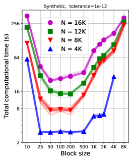
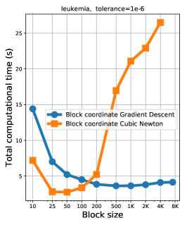
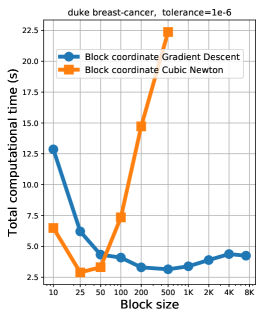
Figure 1: Time it takes to solve a problem for different sampling block sizes. Left: synthetic problem. Center and right: logistic regression for real data.

8.2 Logistic regression

In this experiment we train $\ell_{2}$-regularized logistic regression model for classification task with two classes by its constrained reformulation (16) and compare the Algorithm 1 with the Block coordinate Gradient Descent (see, for example, (Tseng & Yun, 2009)) on the datasets: leukemia ($m=38,d=7129$) and duke breast-cancer ($m=44,d=7129$). We see that using coordinate blocks of size $25-50$ for the Cubic Newton outperforms all other cases of both methods in terms of total computational time. Increasing block size further starts to significantly slow down the method because of high cost of every iteration.

8.3 Poisson regression

In this experiment we train Poisson model for regression task with integer responses by the primal-dual Algorithm 2 and compare it with SDCA (Shalev-Shwartz & Zhang, 2013) and SDNA (Qu et al., 2016) methods on synthetic ($m=1000,d=200$) and real data ($m=319,d=20$). Our approach requires smaller number of epochs to reach given accuracy, but computational efficiency of every step is the same as in SDNA method.

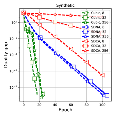
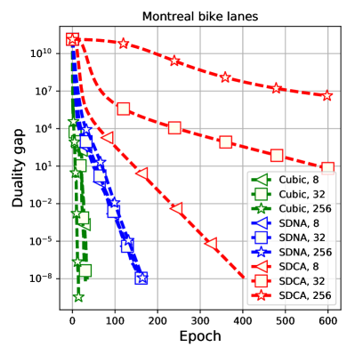
Figure 2: Comparison of Algorithm 2 (marked as Cubic) with SDNA and SDCA methods for minibatch sizes $\tau=8,32,256$, training Poisson regression. Left: synthetic. Right: real data.

In the following set of experiments with Poisson regression we take real datasets: australian ($m=690,d=14$), breast-cancer ($m=683,d=10$), splice ($m=1000,d=60$), svmguide3 ($m=1243,d=21$) and use for response a random vector $y\in(\mathbb{N}\cup\{0\})^{m}$ from the standard Poisson distribution.

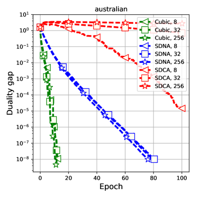
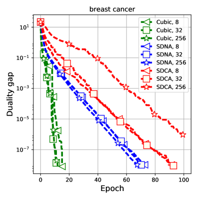
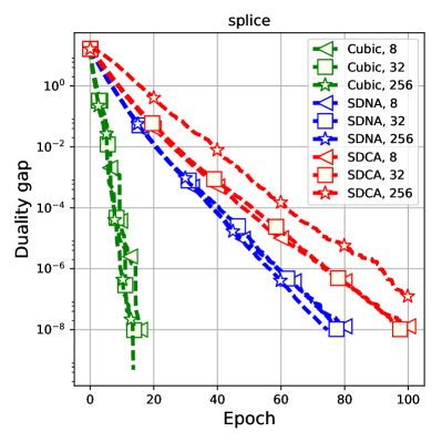
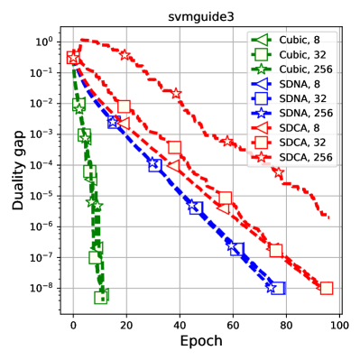
Figure 3: Comparison of Algorithm 2 (marked as Cubic) with SDNA and SDCA methods for minibatch sizes $\tau=8,32,256$, training Poisson regression.

We see that in all the cases our method (Algorithm 2) outperforms state-of-the-art analogues in terms of number of data accesses.

8.4 Experimental setup

In all our experiments we use $\tau$-nice sampling, i.e., subsets of fixed size chosen from all such subset uniformly at random (note that such subsets overlap).

In the experiments with synthetic cubically regularized regression we generate a data in the following way: sample firstly a matrix $U\in\mathbb{R}^{10\times N}$, each entry of which is identically distributed from $\mathcal{N}(0,1)$, then put $A:=U^{T}U\in\mathbb{R}^{N\times N}$, $b:=-U^{T}\xi$, where $\xi\in\mathbb{R}^{10}$ is a normal vector: $\xi_{i}\sim\mathcal{N}(0,1)$ for each $1\leq i\leq 10$, and $c_{j}:=1+|v_{j}|$ where $v_{j}\sim\mathcal{N}(0,1)$ for all $1\leq j\leq N$. Running Algorithm 1 we use for $H_{k}$ the known Lipschitz constants of the Hessians: $H_{k}:=\max_{i\in S_{k}}c_{i}$.

In the experiments with $\ell_{2}$-regularized logistic regression we use the Armijo rule for computing step length in the Block coordinate gradient descent and the constant choice for the parameters $H_{k}$ in Algorithm 1 provided by Proposition 1.

In the experiments with Poisson regression for the methods SDNA and SDCA we use damped Newton method as a computational subroutine to compute one method step, using it until reaching $10^{-12}$ accuracy for the norm of the gradient in the corresponding subproblem and the same accuracy for solving inner cubic subproblem in Algorithm 2. For the synthetic experiment with Poisson regression, we generate data matrix $B\in\mathbb{R}^{m\times d}$ as independent samples from standard normal distribution $\mathcal{N}(0,1)$ and corresponding vector of responses $y\in(\mathbb{N}\cup\{0\})^{m}$ from the standard Poisson distribution (in which mean parameter equals to $1$).

9 Acknowledgments

The work of the first author was partly supported by Samsung Research, Samsung Electronics, the Russian Science Foundation Grant 17-11-01027 and KAUST.

Appendix A Proof of Lemma 1

Proof: Let us show that the Hessian of $\phi_{S}(x)$ is Lipschitz-continuous with a constant $\displaystyle\max_{i\in S}\{\mathcal{H}_{i}\}$. Then (1) will be fulfilled (see Lemma 1 in (Nesterov & Polyak, 2006)). So,

$$\bigl{\|}\nabla^{2}\phi_{S}(x+h)-\nabla^{2}\phi_{S}(x)\bigr{\|}^{2}\;=\;\max_{\|y\|=1}\bigl{\|}\bigl{(}\nabla^{2}\phi_{S}(x+h)-\nabla^{2}\phi_{S}(x)\bigr{)}y\bigr{\|}^{2}$$

$$=\;\max_{\|y\|=1}\sum_{i\in S}\bigl{\|}\bigl{(}\nabla^{2}\phi_{i}(x_{(i)}+h_{(i)})-\nabla^{2}\phi_{i}(x_{(i)})\bigr{)}y_{(i)}\bigr{\|}^{2}$$

$$\overset{\eqref{SmoothnessPhi}}{\leq}\;\max_{\|y\|=1}\sum_{i\in S}\Bigl{(}\mathcal{H}_{i}^{2}\cdot\|h_{(i)}\|^{2}\cdot\|y_{(i)}\|^{2}\Bigr{)}$$

$$=\;\max_{i\in S}\Bigl{\{}\mathcal{H}_{i}^{2}\cdot\|h_{(i)}\|^{2}\Bigr{\}}\;\leq\;\max_{i\in S}\{\mathcal{H}_{i}^{2}\}\cdot\|h_{[S]}\|^{2}.$$

 

Appendix B Auxiliary Results

Lemma 4

Let Assumptions 1, 2, 3, 4 hold. Let minimum of problem (1) exist, and let $x^{*}\in Q$ be its arbitrary solution: $F(x^{*})=F^{*}$.

Then for the random sequence $\{F(x^{k})\}_{k\geq 0}$ generated by Algorithm 1 we have a bound:

$$\mathbb{E}\bigl{[}F(x^{k+1})\,|\,x^{k}\bigr{]}\; \leq\;F(x^{k})\;-\;\frac{\alpha\tau}{n}\Bigl{(}F(x^{k})-F^{*}\Bigr{)}$$

$$-\;\frac{\alpha}{2}\Bigl{\langle}\Bigl{(}\frac{\tau}{n}{\bf G}-\alpha\mathbb{E}\bigl{[}{\bf A}_{[S_{k}]}\bigr{]}\Bigr{)}(x^{k}-x^{*}),x^{k}-x^{*}\Bigr{\rangle}\;+\;\frac{\alpha^{3}\tau}{n}\cdot\frac{\mathcal{H}_{\!F}}{2}\cdot\|x^{k}-x^{*}\|^{3},$$ (19)

for all $\alpha\in[0,1]$.

Proof: From Assumption 1 we have the following bound, ${\bf G}\succeq 0$:

$$\langle\nabla g(x),z\rangle\;\leq\;g(x+z)-g(x)-\frac{1}{2}\langle{\bf G}z,z\rangle,\qquad x,z\in\mathbb{R}^{N}.$$ (20)

Denote $h^{k}\equiv T_{H_{k},S_{k}}(x^{k})$. Then $x^{k+1}=x^{k}+h^{k}$. By a way of choosing $H_{k}$ we have:

$$F(x^{k+1})\quad\leq\quad M^{*}_{H_{k},S_{k}}(x^{k})$$

$$\quad\equiv\quad F(x^{k})\;+\;\langle(\nabla g(x^{k}))_{[S_{k}]},h^{k}\rangle\;+\;\frac{1}{2}\langle{\bf A}_{[S_{k}]}h^{k},h^{k}\rangle\;$$

$$+\;\frac{1}{2}\sum_{i\in S_{k}}\Bigl{(}\langle\nabla\phi_{i}(x_{(i)}^{k}),h_{(i)}^{k}\rangle+\nabla^{2}\phi_{i}(x_{(i)}^{k})h_{(i)}^{k},h_{(i)}^{k}\rangle\Bigr{)}\;+\;\frac{H_{k}}{6}\|h_{[S_{k}]}^{k}\|^{3}\;$$

$$+\;\sum_{i\in S_{k}}\Bigl{(}\psi_{i}(x_{(i)}^{k}+h_{(i)}^{k})\;-\;\psi_{i}(x_{(i)}^{k})\Bigr{)}.$$

At the same time, because $h^{k}$ is a minimizer of the cubic model $M_{H_{k},S_{k}}(x^{k},y)$, we can change $h^{k}$ in the previous bound to arbitrary $y\in\mathbb{R}^{N}$, such that $x^{k}+y\in Q$:

$$F(x^{k+1})\quad\leq\quad F(x^{k})\;+ \;\langle(\nabla g(x^{k}))_{[S_{k}]},y\rangle\;+\;\frac{1}{2}\langle{\bf A}_{[S_{k}]}y,y\rangle\;+\;\sum_{i\in S_{k}}\Bigl{(}\langle\nabla\phi_{i}(x_{(i)}^{k}),y_{(i)}\rangle+\frac{1}{2}\langle\nabla^{2}\phi_{i}(x_{(i)}^{k})y_{(i)},y_{(i)}\rangle\Bigr{)}$$

$$\qquad+\quad\frac{H_{k}}{6}\|y_{[S_{k}]}\|^{3}+\sum_{i\in S_{k}}\Bigl{(}\psi_{i}(x_{(i)}^{k}+y_{(i)})-\psi_{i}(x_{(i)}^{k})\Bigr{)}$$

$$\leq\quad F(x^{k})\;+ \;\langle(\nabla g(x^{k}))_{[S_{k}]},y\rangle\;+\;\frac{1}{2}\langle{\bf A}_{[S_{k}]}y,y\rangle\;+\;\sum_{i\in S_{k}}\Bigl{(}\phi_{i}(x_{(i)}^{k}+y_{(i)})-\phi_{i}(x_{(i)}^{k})\Bigr{)}$$

$$\qquad+\quad\frac{H_{k}+\mathcal{H}_{\!F}}{6}\|y_{[S_{k}]}\|^{3}\;+\;\sum_{i\in S_{k}}\Bigl{(}\psi_{i}(x_{(i)}^{k}+y_{(i)})-\psi_{i}(x_{(i)}^{k})\Bigr{)},$$ (21)

where the last inequality is given by Lemma 1. Note that

$$\mathbb{E}\bigl{[}\|y_{[S_{k}]}\|^{3}\bigr{]}\;\leq\;\mathbb{E}\bigl{[}\|y\|\cdot\|y_{[S_{k}]}\|^{2}\bigr{]}\;=\;\|y\|\cdot\mathbb{E}\Biggl{[}\sum_{i\in S_{k}}\|y_{(i)}\|^{2}\Biggr{]}\;=\;\|y\|\cdot\Biggl{(}\frac{\tau}{n}\sum_{i=1}^{n}\|y_{(i)}\|^{2}\Biggr{)}\;=\;\frac{\tau}{n}\|y\|^{3}.$$

Thus, by taking conditional expectation $\mathbb{E}\bigl{[}\cdot\,|\,x^{k}\bigr{]}$ from (B) we have

$$\mathbb{E}\bigl{[}F(x^{k+1})\,|\,x^{k}\bigr{]}\quad\leq\quad F(x^{k})\;+ \;\frac{\tau}{n}\langle\nabla g(x^{k}),y\rangle\;+\;\frac{1}{2}\langle\mathbb{E}\bigl{[}{\bf A}_{[S_{k}]}\bigr{]}y,y\rangle$$

$$+ \;\frac{\tau}{n}\sum_{i=1}^{n}\Bigl{(}\phi_{i}(x_{(i)}^{k}+y_{(i)})\;+\;\psi_{i}(x_{(i)}^{k}+y_{(i)})\;-\;\phi_{i}(x_{(i)}^{k})\;-\;\psi_{i}(x_{(i)}^{k})\Bigr{)}\;+\;\frac{\tau}{n}\cdot\frac{\mathcal{H}_{\!F}}{2}\|y\|^{3},$$

which is valid for arbitrary $y\in\mathbb{R}^{N}$ such that $x^{k}+y\in Q$. Restricting $y$ to the segment: $y=\alpha(x^{*}-x^{k})$, where $\alpha\in[0,1]$, by convexity of $\phi_{i}$ and $\psi_{i}$ we get:

$$\mathbb{E}\bigl{[}F(x^{k+1})\,|\,x^{k}\bigr{]}\quad\leq\quad F(x^{k})\;+ \;\frac{\alpha\tau}{n}\langle\nabla g(x^{k}),x^{*}-x^{k}\rangle\;+\;\frac{\alpha^{2}}{2}\langle\mathbb{E}\bigl{[}{\bf A}_{S_{k}}\bigr{]}x^{*}-x^{k},x^{*}-x^{k}\rangle$$

$$+ \;\frac{\alpha\tau}{n}\sum_{i=1}^{n}\Bigl{(}\phi_{i}(x^{*}_{(i)})+\psi_{i}(x^{*}_{(i)})-\phi_{i}(x^{k}_{(i)})-\psi_{i}(x^{k}_{(i)})\Bigr{)}\;+\;\frac{\alpha^{3}\tau}{n}\cdot\frac{\mathcal{H}_{\!F}}{2}\|x^{*}-x^{k}\|^{3}.$$

Finally, using inequality (20) for $x\equiv x^{k}$ and $z\equiv x^{*}-x^{k}$ we get the state of the lemma.  

The following technical tool is useful for analyzing a convergence of the random sequence $\xi_{k}\equiv F(x^{k})-F^{*}$ with high probability. It is a generalization of result from (Richtárik & Takáč, 2014).

Lemma 5

Let $\xi_{0}>0$ be a constant and consider a nonnegative nonincreasing sequence of random variables $\{\xi_{k}\}_{k\geq 0}$ with the following property, for all $k\geq 0$:

$$\mathbb{E}\bigl{[}\xi_{k+1}\,|\,\xi_{k}\bigr{]}\;\leq\;\xi_{k}-\frac{\xi_{k}^{p}}{c},$$ (22)

where $c>0$ is a constant and $p\in\{3/2,\,2\}$. Choose confidence level $\rho\in(0,1)$.

Then if we set $0<\varepsilon<\min\{\xi_{0},c^{1/(p-1)}\}$ and

$$K\;\geq\;\frac{c}{\varepsilon^{p-1}}\biggl{(}\frac{1}{p-1}+\log\frac{1}{\rho}\biggr{)}-\frac{c}{\xi_{0}^{p-1}(p-1)},$$ (23)

we have

$$\mathbb{P}(\xi_{K}\leq\varepsilon)\;\geq\;1-\rho.$$ (24)

Proof: Technique of the proof is similar to corresponding one of Theorem 1 from (Richtárik & Takáč, 2014). For a fixed $0<\varepsilon<\min\{\xi_{0},c^{1/(p-1)}\}$ define a new sequence of random variables $\{\xi_{k}^{\varepsilon}\}_{k\geq 0}$ by the following way:

$$\xi_{k}^{\varepsilon}\;=\;\begin{cases}\xi_{k},\;&\text{if}\;\xi_{k}>\varepsilon,\\ 0,\;&\text{otherwise}.\end{cases}$$

It satisfies

$$\xi_{k}^{\varepsilon}\leq\varepsilon\quad\Leftrightarrow\quad\xi_{k}\leq\varepsilon,\qquad k\geq 0,$$

therefore, by Markov inequality:

$$\mathbb{P}(\xi_{k}>\varepsilon)\;=\;\mathbb{P}(\xi_{k}^{\varepsilon}>\varepsilon)\;\leq\;\frac{\mathbb{E}[\xi_{k}^{\varepsilon}]}{\varepsilon},$$

and hence it suffices to show that

$$\theta_{K}\leq\rho\varepsilon,$$

where $\theta_{k}\stackrel{{\scriptstyle\mathrm{def}}}{{=}}\mathbb{E}[\xi_{k}^{\varepsilon}]$. From the conditions of the lemma we get

$$\mathbb{E}\bigl{[}\xi_{k+1}^{\varepsilon}\,|\,\xi_{k}^{\varepsilon}\bigr{]}\;\leq\;\xi_{k}^{\varepsilon}-\frac{(\xi_{k}^{\varepsilon})^{p}}{c},\qquad\mathbb{E}\bigl{[}\xi_{k+1}^{\varepsilon}\,|\,\xi_{k}^{\varepsilon}\bigr{]}\;\leq\;\Bigl{(}1-\frac{\varepsilon^{p-1}}{c}\Bigr{)}\xi_{k}^{\varepsilon},\qquad k\geq 0,$$

and by taking expectations and using convexity of $t\mapsto t^{p}$ for $p>1$ we obtain

$$\theta_{k+1}\quad \leq\quad\theta_{k}-\frac{\theta_{k}^{p}}{c},\qquad k\geq 0,$$ (25)

$$\theta_{k+1}\quad \leq\quad\biggl{(}1-\frac{\varepsilon^{p-1}}{c}\biggr{)}\theta_{k},\qquad k\geq 0.$$ (26)

Consider now two cases, whether $p=2$ or $p=3/2$, and find a number $k_{1}$ for which we get $\theta_{k_{1}}\leq\varepsilon$.

1. $p=2$, then

   $$\frac{1}{\theta_{k+1}}-\frac{1}{\theta_{k}}\;=\;\frac{\theta_{k}-\theta_{k+1}}{\theta_{k+1}\theta_{k}}\;\geq\;\frac{\theta_{k}-\theta_{k+1}}{\theta_{k}^{2}}\;\overset{\eqref{FirstThetaBound}}{\geq}\;\frac{1}{c},$$

   thus we have $\frac{1}{\theta_{k}}\geq\frac{1}{\theta_{0}}+\frac{k}{c}=\frac{1}{\xi_{0}}+\frac{k}{c}$, and choosing $k_{1}\geq\frac{c}{\varepsilon}-\frac{c}{\xi_{0}}$ we obtain $\theta_{k_{1}}\leq\varepsilon$.

2. $p=3/2$, then

   $$\frac{1}{\theta_{k+1}^{1/2}}-\frac{1}{\theta_{k}^{1/2}}\;=\;\frac{\theta_{k}^{1/2}-\theta_{k+1}^{1/2}}{\theta_{k+1}^{1/2}\theta_{k}^{1/2}}\;=\;\frac{\theta_{k}-\theta_{k+1}}{(\theta_{k}^{1/2}+\theta_{k+1}^{1/2})\theta_{k+1}^{1/2}\theta_{k}^{1/2}}\;\geq\;\frac{\theta_{k}-\theta_{k+1}}{2\theta_{k}^{3/2}}\;\overset{\eqref{FirstThetaBound}}{\geq}\;\frac{1}{2c},$$

   thus we have $\frac{1}{\theta_{k}^{1/2}}\geq\frac{1}{\theta_{0}^{1/2}}+\frac{k}{2c}$, and choosing $k_{1}\geq\frac{2c}{\varepsilon^{1/2}}-\frac{2c}{\xi_{0}^{1/2}}$ we get $\theta_{k_{1}}\leq\varepsilon$.

Therefore, for both cases $p\in\{3/2,2\}$ it is enough to choose

$$k_{1}\quad\geq\quad\frac{c}{p-1}\biggl{(}\frac{1}{\varepsilon^{p-1}}-\frac{1}{\xi_{0}^{p-1}}\biggr{)},$$

for which we get $\theta_{k_{1}}\leq\varepsilon$. Finally, letting $k_{2}\geq\frac{c}{\varepsilon^{p-1}}\log\frac{1}{\rho}$ and $K\geq k_{1}+k_{2}$, we have

$$\theta_{K}\;\leq\;\theta_{k_{1}+k_{2}}\;\overset{\eqref{SecondThetaBound}}{\leq}\;\biggl{(}1-\frac{\varepsilon^{p-1}}{c}\biggr{)}^{k_{2}}\theta_{k_{1}}\;\leq\;\exp\biggl{(}-\frac{k_{2}\varepsilon^{p-1}}{c}\biggr{)}\theta_{k_{1}}\;\leq\;\rho\varepsilon.$$

 

Appendix C Proof of Theorem 1

Proof: From bound (4), using ${\bf G}\succeq 0$ and $\mathbb{E}\bigl{[}{\bf A}_{[S_{k}]}\bigr{]}\preceq\frac{\tau L}{n}{\bf I}$ we get, for all $\alpha\in[0,1]$:

$$\mathbb{E}\bigl{[}F(x^{k+1})\,|\,x^{k}\bigr{]}\;\leq\;F(x^{k})-\frac{\alpha\tau}{n}\Bigl{(}F(x^{k})-F^{*}\Bigr{)}\;+\;\frac{\alpha^{2}\tau}{2n}\biggl{(}L\|x^{k}-x^{*}\|^{2}+\alpha\mathcal{H}_{\!F}\|x^{k}-x^{*}\|^{3}\biggr{)}.$$

Thus, for the random sequence $\xi_{k}\equiv F(x^{k})-F^{*}$ we have a bound, for all $\alpha\in[0,1]$:

$$\mathbb{E}\bigl{[}\xi_{k+1}\,|\,\xi_{k}\bigr{]}\;\leq\;\xi_{k}-\frac{\alpha\tau\xi_{k}}{n}+\frac{\alpha^{2}\tau}{2n}D_{0},$$ (27)

where $D_{0}\equiv\max\bigl{\{}LD^{2}+\mathcal{H}_{\!F}D^{3},\,\xi_{0}\bigr{\}}$. Minimum of the right hand side is attained at $\alpha^{*}=\frac{\xi_{k}}{D_{0}}\leq 1$, which substituting to (27) gives: $\mathbb{E}[\xi_{k+1}|\xi_{k}]\;\leq\;\xi_{k}-\frac{\tau\xi_{k}^{2}}{2nD_{0}}$. Applying Lemma 5 complete the proof.  

Appendix D Proof of Theorem 2

Proof: From bound (4), restricting $\alpha$ to the segment$\,[0,\sigma]$ and using (12) we get:

$$\mathbb{E}\bigl{[}\xi_{k+1}\,|\,\xi_{k}\bigr{]}\;\leq\;\xi_{k}-\frac{\alpha\tau\xi_{k}}{n}+\frac{\alpha^{3}\tau}{2n}\mathcal{H}_{\!F}\|x^{k}-x^{*}\|^{3},$$ (28)

where $\xi_{k}\equiv F(x^{k})-F^{*}$ as before. To get the first complexity bound, we rough the right hand side, denoting $D_{0}\equiv\max\bigl{\{}\mathcal{H}_{\!F}D^{3},\xi_{0}\bigr{\}}$:

$$\mathbb{E}\bigl{[}\xi_{k+1}\,|\,\xi_{k}\bigr{]}\;\leq\;\xi_{k}-\frac{\alpha\tau\xi_{k}}{n}+\frac{\alpha^{3}\tau}{2n}\frac{D_{0}}{\sigma^{2}},$$

minimum of which is attained at $\alpha^{*}=\sigma\sqrt{\frac{2}{3}\frac{\xi_{k}}{D_{0}}}\leq\sigma$. Therefore we obtain

$$\mathbb{E}[\xi_{k+1}|\xi_{k}]\;\leq\;\xi_{k}-(2/3)^{3/2}\frac{\tau\sigma\xi_{k}^{3/2}}{nD_{0}},$$

and applying Lemma 5 complete the proof.  

Appendix E Proof of Theorem 3

Proof: Because of strong convexity we know that $\beta>0$ and all the conditions of Theorem 2 are satisfied. Using inequality $F(x^{k})-F^{*}\geq\frac{\mu}{2}\|x^{k}-x^{*}\|^{2}$ for (28), we have for every $\alpha\in[0,\sigma]$:

$$\mathbb{E}\bigl{[}\xi_{k+1}\,|\,\xi_{k}\bigr{]}\;\leq\;\biggl{(}1-\frac{\alpha\tau}{n}+\frac{\alpha^{3}\tau}{n}\frac{\mathcal{H}_{\!F}D}{\mu}\biggr{)}\xi_{k}.$$

Minimum of the right hand side is attained at $\alpha^{*}=\sigma\min\bigl{\{}\sqrt{\frac{\mu}{3\mathcal{H}_{\!F}D}},1\bigr{\}}$, substituting of which and taking total expectation gives a recurrence

$$\mathbb{E}\bigl{[}\xi_{k+1}\bigr{]}\; \leq\;\Biggl{(}\,1-\frac{2\tau\sigma}{3n}\sqrt{\min\Bigl{\{}\frac{\mu}{\mathcal{H}_{\!F}D},1\Bigr{\}}}\,\Biggr{)}\mathbb{E}\bigl{[}\xi_{k}\bigr{]}\;\leq\;\dots\;\leq\;\Biggl{(}\,1-\frac{2\tau\sigma}{3n}\sqrt{\min\Bigl{\{}\frac{\mu}{\mathcal{H}_{\!F}D},1\Bigr{\}}}\,\Biggr{)}^{\!k}\xi_{0}$$

$$\leq\;\exp\Biggl{(}\,-(k+1)\frac{2\tau\sigma}{3n}\sqrt{\min\Bigl{\{}\frac{\mu}{\mathcal{H}_{\!F}D},1\Bigr{\}}}\,\Biggr{)}\xi_{0}.$$

Thus, choosing $K$ large enough, by Markov inequality we have $\mathbb{P}(\xi_{K}>\varepsilon)\;\leq\;\mathbb{E}[\xi_{K}]\varepsilon^{-1}\;\overset{\eqref{Theorem:StronglyConvexLinearRate}}{\leq}\;\rho.$  

Appendix F Proof of Lemma 3

Using notation from the statement of the lemma and multiplying everything by $m$, we can formulate our target optimization subproblem as follows:

$$\min_{\begin{subarray}{c}x\in\mathbb{R}^{|S|},h\in\mathbb{R}^{m}\\ \text{s.t.}\;h=\hat{{\bf B}}x\end{subarray}}\biggl{[}m\lambda\langle b_{1},x\rangle\;+\;\frac{m\lambda}{2}\langle\hat{{\bf A}}x,x\rangle\;+\;\langle b_{2},h\rangle\;+\;\frac{1}{2}\langle{\bf D}h,h\rangle\;+\;\frac{H}{6}\|h\|^{3}\biggr{]},$$ (29)

where ${\bf D}\in\mathbb{R}^{m\times m}$ is a diagonal matrix: ${\bf D}\equiv\operatorname{diag}(\phi_{i}^{\prime\prime}(\alpha_{i}))$. We also denote a subvector of $y$ as $x$ to avoid confusion. The minimum of (29) satisfies the following KKT system:

$$\begin{cases}&m\lambda b_{1}\;+\;m\lambda\hat{{\bf A}}x\;+\;\hat{{\bf B}}^{T}\mu\;=\;0,\\[5.0pt] &b_{2}\;+\;{\bf D}h\;+\;\frac{H}{2}\|h\|h\;-\;\mu\;=\;0,\\[5.0pt] &h\;=\;\hat{{\bf B}}x,\end{cases}$$ (30)

where $\mu\in\mathbb{R}^{m}$ is a vector of slack variables. From the second and the third equations we get:

$$\mu\;=\;b_{2}\;+\;{\bf D}\hat{B}x\;+\;\frac{H}{2}\|\hat{{\bf B}}x\|\hat{{\bf B}}x,$$

plugging of which into the first one gives:

$$\underbrace{\biggl{(}m\lambda\hat{{\bf A}}\;+\;\hat{{\bf B}}^{T}\Bigl{(}{\bf D}+\frac{H}{2}\|\hat{{\bf B}}x\|\Bigr{)}\hat{{\bf B}}\biggr{)}}_{\equiv\;{\bf Z}(\|\hat{{\bf B}}x\|)}\,x\;=\;-\,\underbrace{(m\lambda b_{1}+\hat{{\bf B}}^{T}b_{2})}_{\equiv\;b}.$$

Thus, if we have a solution $\tau^{*}\geq 0$ of the one-dimensional equation:

$$\tau^{*}\;=\;\|\hat{{\bf B}}({\bf Z}(\tau^{*}))^{\dagger}b\|,$$

then we can set

$$x^{*}\;:=\;-({\bf Z}(\tau^{*}))^{\dagger}b,\qquad h^{*}\;:=\;\hat{{\bf B}}x^{*},\qquad\mu^{*}\;:=\;b_{2}+{\bf D}\hat{{\bf B}}x^{*}+\frac{H}{2}\|\hat{{\bf B}}x^{*}\|\hat{{\bf B}}x^{*}.$$

It is easy to check that $(x^{*},h^{*},\mu^{*})$ are solutions of (30) and therefore of (29) as well.

Appendix G Lipschitz Constant of the Hessian of Logistic Loss

Proposition 1

Loss function for logistic regression $\phi(t):=\log(1+\exp(t))$ has Lipschitz-continuous Hessian with constant $\mathcal{H}_{\phi}=1/(6\sqrt{3})$. Thus, it holds, for all $t,s\in\mathbb{R}$:

$$|\phi^{\prime\prime}(t)-\phi^{\prime\prime}(s)|\quad\leq\quad\mathcal{H}_{\phi}|t-s|.$$ (31)

Proof:

To prove (31) it is enough to show: $|\phi^{\prime\prime\prime}(t)|\leq\mathcal{H}_{\phi},$ for all $t\in\mathbb{R}$. Direct calculations give:

$$\phi^{\prime}(t)\;=\;\frac{1}{1+\exp(-t)},\qquad\phi^{\prime\prime}(t)\;=\;\phi^{\prime}(t)\cdot(1-\phi^{\prime}(t)),\qquad\phi^{\prime\prime\prime}(t)\;=\;\phi^{\prime\prime}(t)\cdot(1-2\phi^{\prime}(t)).$$

Let us find extreme values of the function $g(t):=\phi^{\prime\prime\prime}(t)$ for which we have $\displaystyle\lim_{t\to-\infty}g(t)\,=\lim_{t\to+\infty}g(t)=0$.

Stationary points of $g(t)$ are solutions of the equation

$$g^{\prime}(t^{*})\;=\;\phi^{(4)}(t^{*})\;=\;\phi^{\prime\prime}(t^{*})\cdot\bigl{[}(1-2\phi^{\prime}(t^{*}))^{2}-2\phi^{\prime}(t^{*})\cdot(1-\phi^{\prime}(t^{*}))\bigr{]}\;=\;0$$

which consequently should satisfy $\phi^{\prime}(t^{*})=\frac{1}{2}\pm\frac{1}{\sqrt{12}}$ and therefore:

$$g(t^{*})\;=\;\phi^{\prime\prime\prime}(t^{*})\;=\;\biggl{(}\frac{1}{2}+\frac{1}{\sqrt{12}}\biggr{)}\cdot\biggl{(}\frac{1}{2}-\frac{1}{\sqrt{12}}\biggr{)}\cdot\biggl{(}\pm\frac{1}{\sqrt{3}}\biggr{)}\;=\;\pm\frac{1}{6\sqrt{3}},$$

from what we get: $|\phi^{\prime\prime\prime}(t)|\leq 1/(6\sqrt{3})$.

References

- Agarwal et al. (2016) Agarwal, N., Allen-Zhu, Z., Bullins, B., Hazan, E., and Ma, T. Finding approximate local minima for nonconvex optimization in linear time. arXiv preprint arXiv:1611.01146, 2016.
- Bertsekas (1978) Bertsekas, D. P. Local convex conjugacy and Fenchel duality. In Preprints of 7th Triennial World Congress of IFAC, Helsinki, Finland, volume 2, pp. 1079–1084, 1978.
- Carmon & Duchi (2016) Carmon, Y. and Duchi, J. C. Gradient descent efficiently finds the cubic-regularized non-convex newton step. arXiv preprint arXiv:1612.00547, 2016.
- Cartis & Scheinberg (2018) Cartis, C. and Scheinberg, K. Global convergence rate analysis of unconstrained optimization methods based on probabilistic models. Mathematical Programming, 169(2):337–375, 2018.
- Cartis et al. (2011a) Cartis, C., Gould, N. I., and Toint, P. L. Adaptive cubic regularisation methods for unconstrained optimization. part I: motivation, convergence and numerical results. Mathematical Programming, 127(2):245–295, 2011a.
- Cartis et al. (2011b) Cartis, C., Gould, N. I., and Toint, P. L. Adaptive cubic regularisation methods for unconstrained optimization. part II: worst-case function-and derivative-evaluation complexity. Mathematical programming, 130(2):295–319, 2011b.
- Conn et al. (2000) Conn, A. R., Gould, N. I., and Toint, P. L. Trust region methods. SIAM, 2000.
- Ghadimi et al. (2017) Ghadimi, S., Liu, H., and Zhang, T. Second-order methods with cubic regularization under inexact information. arXiv preprint arXiv:1710.05782, 2017.
- Gould et al. (2010) Gould, N. I., Robinson, D. P., and Thorne, H. S. On solving trust-region and other regularised subproblems in optimization. Mathematical Programming Computations, 2(1):21–57, 2010.
- Grapiglia & Nesterov (2017) Grapiglia, G. N. and Nesterov, Y. Regularized Newton methods for minimizing functions with Hölder continuous Hessians. SIAM Journal on Optimization, 27(1):478–506, 2017.
- Griewank (1981) Griewank, A. The modification of Newton’s method for unconstrained optimization by bounding cubic terms. Technical report, Technical Report NA/12, Department of Applied Mathematics and Theoretical Physics, University of Cambridge, 1981.
- Kohler & Lucchi (2017) Kohler, J. M. and Lucchi, A. Sub-sampled cubic regularization for non-convex optimization. arXiv preprint arXiv:1705.05933, 2017.
- Mutnỳ & Richtárik (2018) Mutnỳ, M. and Richtárik, P. Parallel stochastic newton method. Journal of Computational Mathematics, 36(3), 2018.
- Nesterov (2004) Nesterov, Y. Introductory lectures on convex optimization., 2004.
- Nesterov (2007) Nesterov, Y. Modified gauss–newton scheme with worst case guarantees for global performance. Optimisation Methods and Software, 22(3):469–483, 2007.
- Nesterov (2008) Nesterov, Y. Accelerating the cubic regularization of Newton’s method on convex problems. Mathematical Programming, 112(1):159–181, 2008.
- Nesterov (2013) Nesterov, Y. Gradient methods for minimizing composite functions. Mathematical Programming, 140(1):125–161, 2013.
- Nesterov & Polyak (2006) Nesterov, Y. and Polyak, B. T. Cubic regularization of Newton’s method and its global performance. Mathematical Programming, 108(1):177–205, 2006.
- Pilanci & Wainwright (2015) Pilanci, M. and Wainwright, M. J. Randomized sketches of convex programs with sharp guarantees. IEEE Transactions on Information Theory, 61(9):5096–5115, 2015.
- Qu & Richtárik (2016) Qu, Z. and Richtárik, P. Coordinate descent with arbitrary sampling II: expected separable overapproximation. Optimization Methods and Software, 31(5):858–884, 2016.
- Qu et al. (2016) Qu, Z., Richtárik, P., Takáč, M., and Fercoq, O. SDNA: stochastic dual Newton ascent for empirical risk minimization. In International Conference on Machine Learning, pp. 1823–1832, 2016.
- Richtárik & Takáč (2014) Richtárik, P. and Takáč, M. Iteration complexity of randomized block-coordinate descent methods for minimizing a composite function. Mathematical Programming, 144(1-2):1–38, 2014.
- Richtárik & Takáč (2016) Richtárik, P. and Takáč, M. Parallel coordinate descent methods for big data optimization. Mathematical Programming, 156(1-2):433–484, 2016.
- Rockafellar (1997) Rockafellar, R. T. Convex analysis. Princeton landmarks in mathematics, 1997.
- Shalev-Shwartz & Zhang (2013) Shalev-Shwartz, S. and Zhang, T. Stochastic dual coordinate ascent methods for regularized loss minimization. Journal of Machine Learning Research, 14(Feb):567–599, 2013.
- Tripuraneni et al. (2017) Tripuraneni, N., Stern, M., Jin, C., Regier, J., and Jordan, M. I. Stochastic cubic regularization for fast nonconvex optimization. arXiv preprint arXiv:1711.02838, 2017.
- Tseng & Yun (2009) Tseng, P. and Yun, S. A coordinate gradient descent method for nonsmooth separable minimization. Mathematical Programming, 117(1-2):387–423, 2009.