Performance Analysis of Low Latency Multiple Full-Duplex Selective Decode and Forward Relays

Abstract

In order to follow up with mission-critical applications, new features need to be carried to satisfy a reliable communication with reduced latency. With this regard, this paper proposes a low latency cooperative transmission scheme, where multiple full-duplex relays, simultaneously, assist the communication between a source node and a destination node. First, we present the communication model of the proposed transmission scheme. Then, we derive the outage probability closed-form for two cases: asynchronous transmission (where all relays have different processing delay) and synchronous transmissions (where all relays have the same processing delay). Finally, using simulations, we confirm the theoretical results and compare the proposed multi-relays transmission scheme with relay selection schemes.

I Introduction

Future wireless networks, i.e., 5G, open new perspectives and allow the existence of diversified services with the aim of bringing a wide variety of novel applications, among which we distinct mission-critical applications. To ensure the radio communication for such applications, very low latency as well as extreme reliability are required, whence came, the definition of ultra-reliable and low latency communications (URLLC). As one of flexible defined 5G service categories, URLLC needs to be carried in cellular networks in order to enable and support several applications, and targets important sectors namely, health, industry and transportation. However, the requested characteristics or functionalities will not be the same, as each application inquires various performance requirements which makes their setting more conflicting and challenging [1, 2]. In this context, the use of cooperation concept provides spatial and temporal diversity, and constitutes a good alternative to support advanced communications with increased channel capacity [3, 4].

In general, there are various ways of relay processing in cooperative networks, among which we distinct mainly two familiar techniques: amplify-and-forward (AF) and decode-and-forward (DF) [5]. In AF scheme, the relay simply amplifies the received signal and forwards it towards the destination. However, this relaying scheme suffers from noise amplification. In the DF scheme, the relay first decodes the signal received from the source, re-encodes and re-transmits it to the destination. This approach suffers from error propagation when the relay transmits an erroneously decoded data block. Selective DF, where the relay only transmits when it can reliably decode the data packet, has been introduced as an efficient method to reduce error propagation [6]. Overall, all proposed cooperative schemes aim to increase the diversity order of the system, hence, improving the network performance.

Even if the full-duplex (FD) relaying mode generates loop interference from the relay input to the relay output, it still practical to use on cooperative relaying systems due to its spectral efficiency [7, 8]. The FD relay requires the duplication of radio frequency circuits to transmits and receives simultaneously in the same time slot and in the same frequency band. It has been shown that the FD mode still feasible even with the presence of significant loop interference [7], especially with recent advances noted in antenna technology and signal processing techniques. In [9], a novel technique for self-interference cancellation using antenna cancellation was depicted for FD transmissions. In the same context, through passive suppression and active self-interference cancellation mechanisms, an experiment study was proposed in [10]. Hence, these practical growths incite authors to adopt FD communications in their research, thus, get rid of spectral inefficiency caused by half-duplex (HD) relaying mode.

In cooperative systems, one or multiple relays may be used to assist transmission between a source and a destination nodes. The application of the relay selection principle on FD system permits the merging of space diversity as well as the spectral efficiency [11]. Therefore, several works in the literature have considered the relay selection concept applied to their studied multiple relays systems [11, 12, 13]. The best proved relay selection policy for FD cooperative networks is the optimal relay selection (OS) [11, 13]. This scheme takes into consideration the global channel state information (CSI) of the source to relay channels as well as that of the relay to destination channels. So, despite its proved performance, the OS induces more system overhead [11, 14, 15], hence, more system latency. With the aim of reducing the system latency and the implementation complexity, partial relay selection (PS) scheme that requires just the CSI knowledge of one hop, were introduced in [11]. To the best of our knowledge, only few works carried the multiple relays model without relay selection. In [16], the performance of HD multiple decode-and-forward system, were investigated for non identical distributed channels. Recently, FD-AF cooperative system were studied [3]. The authors proposed a forced delayed FD relaying scheme, where an iterative successive interference cancellation model was used to withdraw the accumulation effect between signals at the destination. In this paper, we propose a multiple FD relaying scheme, where non-controlled selective decode and forward (SDF) relays, simultaneously, assist the communication between a source and destination nodes. First, we derive the outage probability closed-form of the proposed system. Then, as a benchmark, we investigate the performances comparison with the OS and the PS relay selection schemes.

The rest of the paper is organized as follows: Section II presents the communication model of the proposed transmission scheme. The outage probability of multiple FD-SDF relays is derived in Section III. In Section IV, Numerical results are shown and discussed. The paper is concluded in Section V.

      Notations

• $x$, $\mathbf{x}$, and $\mathbf{X}$ denote, respectively, a scalar quantity, a column vector, and a matrix.

• $\mathcal{CN}\left(\mu,\sigma\right)$ represents a circularly symmetric complex Gaussian distribution with mean $\mu$ and variance $\sigma$.

• $\delta_{m,n}$ is the Kronecker symbol, i.e., $\delta_{m,n}=1$ for $m=n$ and $\delta_{m,n}=0$ for $m\neq n$.

• $\left(.\right)^{\star}$,$\left(.\right)^{\top}$, and $\left(.\right)^{\mathrm{H}}$ are conjugate, the transpose, and the Hermitian transpose, respectively.

• $\mathbb{C}$ is set of complex number.

• For $\mathbf{x}\in\mathbb{C}^{N\times 1}$, $\mathbf{x}_{f}$ denotes the discrete Fourier transform (DFT) of $\mathbf{x}$, i.e., $\mathbf{x}_{f}=\mathbf{U}_{N}\mathbf{x}$, with $\mathbf{U}_{N}$ is a unitary $N\times N$ matrix whose $\left(m,n\right)$th element is $\left(\mathbf{U}_{N}\right)_{m,n}=\frac{1}{\sqrt{N}}e^{-j(2\pi mn/N)}$, $j=\sqrt{-1}$.

• $\left|.\right|$ denotes the absolute value.

• $\mathbb{{E}}\left\{.\right\}$ is used to denote the statistical expectation.

• $\mathrm{Pr}\left(X\right)$ is the probability of occurrence of the event $X$.

II Communication Model

We consider a multi-relay cooperative system, where a set $\mathcal{R}$ of $N$ FD-relays $(\mathrm{R_{\mathit{k}}})$, $(k=1,...,N)$ assists the communication between a source $(\mathrm{S})$ and a destination $(\mathrm{D})$, as depicted in Fig. 1. Since all relays operate in FD mode, we take into account the residual self-interference (RSI) generated from relay’s input to relay’s output, as well as inter-relay interference (IRI).

The source-destination $\mathrm{S\rightarrow D}$, source-relay $\mathrm{S\rightarrow R_{\mathit{k}}}$, the relay interference $\mathrm{R_{\mathit{k^{\prime}}}\rightarrow R_{\mathit{k}}}$, i.e., RSI $(k=k^{\prime})$ and IRI $(k\neq k^{\prime})$, and relay-destination $\mathrm{R_{\mathit{k}}\rightarrow D}$ channels, are represented by $h_{\mathrm{\mathrm{ab}}},$ with $\mathrm{ab}\,\epsilon\left\{\mathrm{SD},\,\mathrm{SR_{\mathit{k}}},\,\mathrm{R_{\mathit{k^{\prime}}}R_{\mathit{k}}},\,\mathrm{R_{\mathit{k}}D}\right\}$. In this paper, all channels are assumed independent identically distributed (i.i.d.) zero mean circularly symmetric complex Gaussian $\sim\mathcal{CN}(0,\sigma_{\mathrm{ab}}^{2})$. We assume a perfect CSI at the receiver nodes and limited CSI at the transmitter nodes, i.e., the transmitter is only aware of the processing delay at the relay nodes.

In this work, we consider all relays are operating using SDF relaying mode, where the relay transmits only when it can correctly decode the source message. The received signals, at time instance $i$, at relay $\mathrm{R_{\mathit{k}}}$ and destination $\mathrm{D}$ are, respectively, given by

$$y_{\mathrm{\mathrm{R_{\mathit{k}}}}}(i) =\sqrt{P_{\textrm{S}}}h_{\mathrm{SR_{\mathit{k}}}}x_{\mathrm{s}}(i)+\sum_{\mathrm{R}_{\mathit{\mathit{k^{\prime}}}}\in\mathcal{R}_{L}}\sqrt{P_{\mathrm{R}}}h_{\mathrm{R_{\mathit{k^{\prime}}}R_{\mathit{k}}}}x_{\mathrm{s}}(i-\tau_{\mathit{k^{\prime}}})$$ (1)

$$+n_{\mathrm{R_{\mathit{k}}}}(i),$$

$$=\sqrt{P_{\textrm{S}}}h_{\mathrm{SR_{\mathit{k}}}}x_{\mathrm{s}}(i)+\underset{\mathrm{RSI+IRI}}{\underbrace{V_{\mathrm{R}_{\mathit{k}}}(i)}}+n_{\mathrm{R}_{\mathit{k}}}(i),$$

$$y_{\mathrm{D}}(i) =\underset{\mathrm{Direct\,+\,Relayed\,signal}}{\underbrace{\sqrt{P_{\textrm{S}}}h_{\mathrm{SD}}x_{\mathrm{s}}(i)+\sum_{\mathrm{R}_{\mathit{\mathit{k}}}\in\mathcal{R}_{L}}\sqrt{P_{\mathrm{R}}}h_{\mathrm{\mathrm{R}_{\mathit{k}}D}}x_{\mathrm{s}}(i-\tau_{\mathit{k}})}}$$ (2)

$$+\underset{\mathrm{Noise}}{\underbrace{n_{\mathrm{D}}(i)}},$$

where $P_{\textrm{S}}$ and $P_{\mathrm{R}}$ denote, respectively, the transmit power of $\mathrm{S}$ and $\mathrm{R}_{\mathit{\mathit{k}}}$, $x_{\mathrm{s}}(i)$ is the source transmitted signal at channel use $i$ with $\mathbb{{E}}\left[x_{\mathrm{s}}(i)x_{\mathrm{s}}^{\star}(i^{\prime})\right]=\delta_{i,i^{\prime}}$, and $\mathcal{R}_{\mathit{L}}\subset\mathcal{R}$ denotes the set of $L$ relays that correctly decode the source message. $n_{\mathrm{R_{\mathit{k}}}}\sim\mathcal{CN}(0,N_{\mathrm{R}})$ and $n_{\mathrm{D}}\sim\mathcal{CN}(0,N_{\mathrm{D}})$ respectively denote, a zero-mean complex additive white Gaussian noise at the relay $\mathrm{R}_{\mathit{\mathit{k}}}$ and the destination $\mathrm{D}$. Without loss of generality and for the sake of presentation, we assume $N_{\mathrm{D}}=N_{\mathrm{R}}=1$. The processing delay at relay $\mathrm{R}_{\mathit{\mathit{k}}}$ is denoted $\tau_{k}$ , $V_{\mathrm{R}_{\mathit{\mathit{k}}}}(i)$ covers the RSI$+$IRI at a relay $\mathrm{R}_{\mathit{\mathit{k}}}$ after undergoing all known cancellation techniques and practical isolation [8, 17]. $V_{\mathrm{R}_{\mathit{\mathit{k}}}}(i)$ is assumed to be equivalent to a zero mean complex Gaussian random variable $\sim\mathcal{CN}(0,\sigma_{\mathrm{RSI,R_{\mathit{k}}}}^{2}+\sigma_{\mathrm{IRI,R_{\mathit{k}}}}^{2})$, with $\sigma_{\mathrm{RSI,\mathit{k}}}^{2}=\sigma_{\mathrm{R_{\mathit{k}}R_{\mathit{k}}}}^{2}$ and $\sigma_{\mathrm{IRI,\mathit{k}}}^{2}={\displaystyle\sum_{\underset{k^{\prime}\neq k}{\mathrm{R}_{\mathit{\mathit{k^{\prime}}}}\in\mathcal{R}_{L}}}}\sigma_{\mathrm{R_{\mathit{k^{\prime}}}R_{\mathit{k}}}}^{2}$.

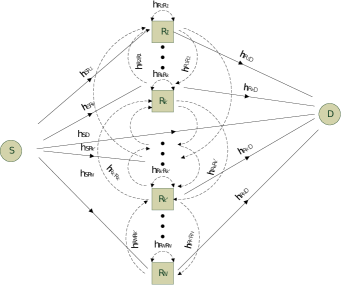
Figure 1: The FD SDF multi-relay system.

From (2), we can see that the destination node will receive the source node transmitted signal $x_{\mathrm{s}}$ at different time instance due to the processing delay $\tau_{k}$ at the relay $\mathrm{R}_{\mathit{k}}$. In order to alleviate the inter-symbol interference (ISI) caused by the delayed signal, equalization is needed at the destination side. For that purpose, we propose a cyclic-prefix (CP) transmission at the source side in order to perform frequency-domain equalization (FDE) at the destination node.

In this paper, we assume that all channel gains change independently from one block to another and remain constant during one block of $T+\tau_{\mathrm{CP}}$ channel uses, where $T$ represents the number of transmitted code-words and $\tau_{\mathrm{CP}}$ the CP length ($\tau_{\mathrm{CP}}\geq\mathit{\underset{k}{\mathrm{max}}\mathrm{(\tau_{\mathit{k}})}}$). Hence, (2) can be rewritten in vector form to jointly take into account the $T+\tau_{\mathrm{CP}}$ received signal as [18]

$$\mathbf{y}_{D}=\boldsymbol{{\mathcal{H}}}\mathbf{x}_{\mathrm{s}}+\mathbf{n},$$ (3)

where $\mathbf{y}_{\mathrm{D}}=\left[y_{\mathrm{D}}\left(0\right),...,y_{\mathrm{D}}\left(T-1\right)\right]^{\top}\in\mathbb{C}^{T\times 1}$, $\mathbf{x}_{\mathrm{s}}=\left[x_{\mathrm{s}}\left(0\right),...,x_{\mathrm{s}}\left(T-1\right)\right]^{\top}\in\mathbb{C}^{T\times 1}$, with $\mathbf{n}=\left[n_{\mathrm{D}}\left(0\right),...,n_{\mathrm{D}}\left(T-1\right)\right]^{\top}\in\mathbb{C}^{T\times 1}$ and $\boldsymbol{{\mathcal{H}}}\in\mathbb{C}^{T\times T}$ is a circulant matrix that can be decomposed as

$$\boldsymbol{{\mathcal{H}}}=\mathbf{U}_{T}^{H}\boldsymbol{{\Lambda}}\mathbf{U}_{T},$$ (4)

where $\boldsymbol{{\Lambda}}$ is a diagonal matrix whose $\left(i,i\right)$-th element is

$$\lambda_{i}=\sqrt{P_{\textrm{S}}}h_{\mathrm{SD}}+{\displaystyle\sum_{\mathrm{R}_{\mathit{\mathit{k}}}\in\mathcal{R}_{L}}}\sqrt{P_{\mathrm{R}}}h_{\mathrm{R_{\mathit{k}}D}}\textrm{e}^{-j\left(2\pi i\frac{\tau_{k}}{T}\right)}.$$ (5)

The signal $\mathbf{y}_{\mathrm{D}}$ can be therefore represented in the frequency domain as

$$\mathbf{y}_{\mathrm{D}_{f}}=\boldsymbol{{\Lambda}}\mathbf{x}_{\mathrm{s}_{f}}+\mathbf{n}_{f}.$$ (6)

At the destination, the instantaneous end-to-end equivalent signal-to-interference and noise ratio (SINR), at frequency bin $i$, is expressed as

$$\gamma_{i}= \lambda_{i}\lambda_{i}^{H}$$ (7)

$$= P_{\textrm{S}}|h_{\mathrm{SD}}|^{2}+\alpha_{L}+A,$$

where $\alpha_{L}=P_{\mathrm{R}}|{\displaystyle\sum_{\mathrm{R}_{\mathit{\mathit{k}}}\in\mathcal{R}_{L}}}h_{\mathrm{R_{\mathit{k}}D}}e^{-j\left(2\pi i\frac{\tau_{k}}{T}\right)}|^{2}$, $A=2\sqrt{P_{\textrm{S}}}\sqrt{P_{\mathrm{R}}}{\displaystyle\sum_{\mathrm{R}_{\mathit{\mathit{k}}}\in\mathcal{R}_{L}}}\left(|h_{\mathrm{SD}}h_{\mathrm{R_{\mathit{k}}D}}^{\text{*}}|\cos\left(2\pi i\frac{\tau_{k}}{T}+\theta_{\mathit{k}}\right)\right)$ and $\theta_{\mathit{k}}=\textrm{angle}\left(h_{\mathrm{SD}}h_{\mathrm{R_{\mathit{k}}D}}^{\text{*}}\right)$.

III Outage Probability

In this section, we derive the proposed transmission scheme outage probability. For that purpose, let’s first introduce the instantaneous SINRs for each link. The received instantaneous SINR of $\mathrm{S}\rightarrow\mathrm{D}$, $\mathrm{S}\rightarrow\mathrm{R_{\mathit{k}}}$ and $\mathrm{R_{\mathit{k}}}\rightarrow\mathrm{D}$ links are, respectively, denoted $\gamma_{\mathrm{SD}}=P_{\textrm{S}}|h_{\mathrm{SD}}|^{2}$, $\gamma_{\mathrm{R_{\mathit{\mathit{k}}}D}}=P_{\mathrm{R}}|h_{\mathrm{R_{\mathit{k}}D}}|^{2}$ and $\gamma_{\mathrm{SR_{\mathit{k}}}}=\frac{P_{\textrm{S}}|h_{\mathrm{\mathrm{SR_{\mathit{k}}}}}|^{2}}{P_{\mathrm{R}}\left(\sigma_{\mathrm{RSI,R_{\mathit{k}}}}^{2}+\sigma_{\mathrm{IRI,R_{\mathit{k}}}}^{2}\right)+1}$. Note that all SINRs are exponentially distributed random variables.

The multiple SDF FD relay system outage probability can be expressed as

$$\mathcal{P}_{out} =P_{out}^{\mathrm{S\rightarrow D}}\underset{\mathrm{R^{{}^{\prime}}}\in\mathit{\mathcal{R}}}{\prod}P_{out}^{\mathrm{S\rightarrow R^{{}^{\prime}}}}$$ (8)

$$+\sum_{L=1}^{N}\mathit{\sum_{\mathcal{R}_{L}}P_{out}^{\mathrm{S}\mathcal{R_{\mathit{L}}}\mathrm{D}}}\underset{\mathrm{R}\in\mathcal{R}_{L}}{\prod}\left(1-P_{out}^{\mathrm{S\rightarrow R}}\right)\underset{\mathrm{R^{{}^{\prime}}}\in\overline{\mathcal{R}}_{L}}{\prod}P_{out}^{\mathrm{S\rightarrow R^{{}^{\prime}}}},$$

where $\mathcal{R}_{L}$ denotes the set of $L$ relays not in outage and $\overline{\mathcal{R}}_{L}\triangleq\mathit{\mathcal{R}}\setminus\mathit{\mathcal{R}}_{L}$. $P_{out}^{\mathrm{S\rightarrow D}}$ and $P_{out}^{\mathrm{S\rightarrow R}}$ denote respectively, the outage probability of $\mathrm{S\rightarrow D}$ link and $\mathrm{S\rightarrow R}$ link, and can be expressed as

$$P_{out}^{\mathrm{S\rightarrow D}}= \mathrm{Pr}(\gamma_{\mathrm{SD}}<\eta)= 1-\textrm{e}^{-\frac{\eta}{P_{\textrm{S}}\sigma_{\mathrm{SD}}^{2}}}$$

$$P_{out}^{\mathrm{S\rightarrow R_{\mathit{k}}}}= \mathrm{Pr}(\gamma_{\mathrm{SR_{\mathit{k}}}}<\eta)= 1-\textrm{e}^{-\frac{\eta\left(P_{\mathrm{R}}\left(\sigma_{\mathrm{RSI,R_{\mathit{k}}}}^{2}+\sigma_{\mathrm{IRI,R_{\mathit{k}}}}^{2}\right)+1\right)}{P_{\textrm{S}}\sigma_{\mathrm{SR}}^{2}}},$$ (9)

where $\eta=2^{r\left(\frac{T+\tau_{CP}}{T}\right)}-1$, with $r$ is the bit rate per channel use. Note that the factor $\frac{T+\tau_{CP}}{T}$ means that the transmission of $T$ useful code-words occupies $T+\tau_{CP}$ channel uses. $P_{out}^{\mathrm{S}\mathcal{R_{\mathit{L}}}\mathrm{D}}$ denotes, the outage probability of a cooperative system where a set $\mathcal{R}_{L}$ of $L$ relays assist the communication between node $\mathrm{S}$ and node $\mathrm{D}$, and it can be derived as follows:

$$P_{out}^{\mathrm{S}\mathcal{R_{\mathit{L}}}\mathrm{D}}=\mathrm{Pr}\left(\frac{1}{T+\tau_{CP}}\sum_{i=0}^{T-1}\log_{2}(1+\gamma_{i})<r\right).$$ (10)

To derive the closed form expression of (10), we consider two cases, i.e., the asynchronous transmission $(\tau_{\mathit{k}}\neq\tau_{\mathit{k^{\prime}}},\,\forall\mathit{k\neq k^{\prime}})$ and the synchronous transmission $(\tau_{\mathit{k}}=\tau_{\mathit{k^{\prime}}}=\tau,\,\forall\mathit{k\neq k^{\prime}})$.

• Asynchronous transmission

In the asynchronous transmission, all relays forward signals to the destination with different delay processing, i.e., $(\tau_{\mathit{k}}\neq\tau_{\mathit{k^{\prime}}},\,\forall\mathit{k\neq k^{\prime}})$. Inspired from [19], we have ${\displaystyle\sum_{i=0}^{T-1}}\log_{2}(1+\gamma_{i})=\sum_{i=0}^{T-1}\log_{2}\left\{\left(1+P_{\textrm{S}}|h_{\mathrm{SD}}|^{2}+\alpha_{L}\right)\times\left(1+\frac{A}{1+P_{\textrm{S}}|h_{\mathrm{SD}}|^{2}+\alpha_{L}}\right)\right\}$, and thereby, we get,

$$\sum_{i=0}^{T-1}\log_{2}(1+\gamma_{i}) =\sum_{i=0}^{T-1}\log_{2}\left(1+P_{\textrm{S}}|h_{\mathrm{SD}}|^{2}+\alpha_{L}\right)$$

$$+\sum_{i=0}^{T-1}\log_{2}\left(1+\frac{A}{1+P_{\textrm{S}}|h_{\mathrm{SD}}|^{2}+\alpha_{L}}\right).$$ (11)

Thanks to arithmetic-geometric mean inequality for complex number, we get $P_{\textrm{S}}|h_{\mathrm{SD}}|^{2}+\alpha_{L}>A$. Thus, using the first Taylor expansion, $\log_{2}\left(1+\frac{A}{1+P_{\textrm{S}}|h_{\mathrm{SD}}|^{2}+\alpha_{L}}\right)\approx\frac{1}{\ln\left(2\right)}\frac{A}{1+P_{\textrm{S}}|h_{\mathrm{SD}}|^{2}+\alpha_{L}}$. Noting that ${\displaystyle\sum_{i=0}^{T-1}}\cos\left(2\pi i\frac{\tau_{k}}{T}+\theta_{k}\right)=0$. Therefore, the second term in (11) vanishes. Thus, (11) can be approximated as

$$\sum_{i=0}^{T-1}\log_{2}(1+\gamma_{i}) \approx\sum_{i=0}^{T-1}\log_{2}\left(1+P_{\textrm{S}}|h_{\mathrm{SD}}|^{2}+\alpha_{L}\right)$$

$$=\sum_{i=0}^{T-1}\log_{2}\left(1+P_{\textrm{S}}|h_{\mathrm{SD}}|^{2}+P_{\mathrm{R}}|h_{\mathrm{R_{\mathit{L}}D}}|^{2}+\alpha_{L-1}\right.$$

$$+\left.\beta_{L}\right)$$

$$=\sum_{i=0}^{T-1}\log_{2}\left(1+P_{\textrm{S}}|h_{\mathrm{SD}}|^{2}+P_{\mathrm{R}}|h_{\mathrm{R_{\mathit{L}}D}}|^{2}+\alpha_{L-1}\right)+$$

$$\sum_{i=0}^{T-1}\log_{2}\left(1+\frac{\beta_{L}}{1+P_{\textrm{S}}|h_{\mathrm{SD}}|^{2}+P_{\mathrm{R}}|h_{\mathrm{R_{\mathit{L}}D}}|^{2}+\alpha_{L-1}}\right),$$ (12)

with $\beta_{L}=2P_{\mathrm{R}}{\displaystyle\sum_{\mathrm{R}_{\mathit{\mathit{k}}}\in\mathcal{R}_{L}}}\left(|h_{\mathrm{R_{\mathit{L}}D}}h_{\mathrm{R_{\mathit{k}}D}}^{\text{*}}|\cos\left(2\pi i\frac{\tau_{L}-\tau_{k}}{T}+\varphi_{L,k}\right)\right)$ and $\varphi_{L,k}=\textrm{angle}\left(h_{\mathrm{R_{\mathit{L}}D}}h_{\mathrm{R_{\mathit{k}}D}}^{\text{*}}\right)$. Noting that $1+P_{\textrm{S}}|h_{\mathrm{SD}}|^{2}+P_{\mathrm{R}}|h_{\mathrm{R_{\mathit{L}}D}}|^{2}+\alpha_{L-1}>P_{\mathrm{R}}|h_{\mathrm{R_{\mathit{L}}D}}|^{2}+\alpha_{L-1}\geq\beta_{L}$ and using the same mathematical manipulations as before, we can easily proof that the second term in (12) vanishes. Repeating the same mathematical manipulations, we found that (12) can be approximated as

$$\sum_{i=0}^{T-1}\log_{2}(1+\gamma_{i})\approx T\log_{2}\left(1+P_{\textrm{S}}|h_{\mathrm{SD}}|^{2}+P_{\mathrm{R}}\sum_{\mathrm{R}_{\mathit{\mathit{k}}}\in\mathcal{R}_{L}}|h_{\mathrm{R_{\mathit{k}}D}}|^{2}\right).$$ (13)

From (13), we can see that using equalization at the destination side, for asynchronous transmission, allows to virtually separate different spatial paths and thereby achieve a full spatial diversity. Therefore, $P_{out}^{\mathrm{S}\mathcal{R_{\mathit{L}}}\mathrm{D}}$ can be derived as

$$P_{out}^{S\mathcal{R_{\mathit{L}}}\mathrm{D}}= \mathrm{Pr}\left(\frac{T}{T+\tau_{CP}}\log_{2}\left(1+\gamma_{\mathrm{SD}}+\sum_{\mathrm{R}_{\mathit{\mathit{k}}}\in\mathcal{R}_{L}}\gamma_{\mathrm{R_{\mathit{\mathit{k}}}D}}\right)<r\right)$$

$$= \mathrm{Pr}\left(\gamma_{\mathrm{SD}}+\sum_{\mathrm{R}_{\mathit{\mathit{k}}}\in\mathcal{R}_{L}}\gamma_{\mathrm{R_{\mathit{\mathit{k}}}D}}<\eta\right)$$

$$= \intop_{0}^{\eta}\mathrm{Pr}\left(\gamma_{\mathrm{SD}}<\eta-y\right)\times f_{{\displaystyle\sum_{\mathrm{R}_{\mathit{\mathit{k}}}\in\mathcal{R}_{L}}}\gamma_{\mathrm{R_{\mathit{\mathit{k}}}D}}}(y)\textrm{d}y.$$ (14)

For simplicity, we consider all relays experience the same $\mathrm{R_{\mathit{k}}}\rightarrow\mathrm{D}$ link quality, i.e., $\sigma_{\mathrm{RD}}^{2}=\sigma_{\mathrm{R_{\mathit{k}}D}}^{2},\>\forall k$. Therefore, ${\displaystyle\sum_{\mathrm{R}_{\mathit{\mathit{k}}}\in\mathcal{R}_{L}}}\gamma_{{}_{\gamma_{\mathrm{R_{\mathit{\mathit{k}}}D}}}}$ follows gamma distribution with parameters $L$ and $\overline{\gamma}_{\mathrm{RD}}=P_{\mathrm{R}}\sigma_{\mathrm{RD}}^{2}$, and with probability distribution function (pdf) $f_{{\displaystyle\sum_{\mathrm{R}_{\mathit{\mathit{k}}}\in\mathcal{R}_{L}}}\gamma_{{}_{\gamma_{\mathrm{R_{\mathit{\mathit{k}}}D}}}}}(x)=\frac{1}{\overline{\gamma}_{\mathrm{RD}}}\textrm{e}^{-\frac{x}{\overline{\gamma}_{\mathrm{RD}}}}\frac{\left(\frac{x}{\overline{\gamma}_{\mathrm{RD}}}\right)^{L-1}}{\left(L-1\right)!}$. So accordingly, after some manipulations, we get the expression of $P_{out}^{\mathrm{S}\mathcal{R_{\mathit{L}}}\mathrm{D}}$ as depicted below:

$$P_{out}^{S\mathcal{R_{\mathit{L}}}D}= \frac{\gamma\left(L,\frac{\eta}{\overline{\gamma}_{\mathrm{RD}}}\right)}{\Gamma(L)}-\frac{\textrm{e}^{-\frac{\eta}{\overline{\gamma}_{\mathrm{SD}}}}}{\Gamma(L)}\times$$

$$\left(\frac{\overline{\gamma}_{\mathrm{SD}}}{\overline{\gamma}_{\mathrm{SD}}-\overline{\gamma}_{\mathrm{RD}}}\right)^{L}\times\gamma\left(L,\eta\frac{\overline{\gamma}_{\mathrm{SD}}-\overline{\gamma}_{\mathrm{RD}}}{\overline{\gamma}_{\mathrm{RD}}\overline{\gamma}_{\mathrm{SD}}}\right),$$ (15)

where $\overline{\gamma}_{\mathrm{SD}}=P_{\textrm{S}}\sigma_{\mathrm{SD}}^{2}$, $\Gamma(L)=\left(L-1\right)!$ is the factorial of $L-1$, and $\gamma(n,x)$ presents the lower incomplete Gamma function which is given by $\intop_{0}^{x}t^{n-1}\textrm{e}^{-t}\textrm{d}t$ [20, 8.350.1]. Thereby, by substituting (9) and (15) into (8), we get the closed form expression of the outage probability for the asynchronous case.

• Synchronous transmission

In the synchronous transmission, all relays forward signals to the destination with the same delay processing. Therefore, $\lambda_{i}$ in (5) can be expressed as $\lambda_{i}=\sqrt{P_{\textrm{S}}}h_{\mathrm{SD}}+\sqrt{P_{\mathrm{R}}}\left({\displaystyle\sum_{\mathrm{R}_{\mathit{\mathit{k}}}\in\mathcal{R}_{L}}}h_{\mathrm{R_{\mathit{k}}D}}\right)\textrm{e}^{-j\left(2\pi i\frac{\tau_{k}}{T}\right)}$. We see clearly that the synchronous transmission is equivalent to one relay system with $\mathrm{R\rightarrow D}$ channel $h_{\mathrm{syn}}={\displaystyle\sum_{\mathrm{R}_{\mathit{\mathit{k}}}\in\mathcal{R}_{L}}}h_{\mathrm{R_{\mathit{k}}D}}\sim\mathcal{CN}(0,{\displaystyle\sum_{\mathrm{R}_{\mathit{\mathit{k}}}\in\mathcal{R}_{L}}}\sigma_{\mathrm{R}_{k}\mathrm{D}}^{2})$ and received instantaneous SINR $\gamma_{\mathrm{syn}}=P_{\mathrm{R}}|h_{\mathrm{syn}}|^{2}$. Thus, synchronous transmission represents the worst scenario where adding more relays does not add any diversity to the system [3].

By referring to the proof in [19], $P_{out}^{\mathrm{S}\mathcal{R_{\mathit{L}}}\mathrm{D}}$ can be derived as

$$P_{out}^{\mathrm{S}\mathcal{R_{\mathit{L}}}\mathrm{D}}\approx \mathrm{Pr}\left(\frac{T}{T+\tau_{\mathrm{CP}}}\log_{2}(1+\gamma_{\mathrm{SD}}+\gamma_{\mathrm{syn}})<r\right)$$ (16)

$$= \mathrm{Pr}\left(\gamma_{\mathrm{SD}}+\gamma_{\mathrm{syn}}<\eta\right)$$

$$= \intop_{0}^{\eta}\mathrm{Pr}\left(\gamma_{\mathrm{SD}}<\eta-y\right)\times f_{\gamma_{\mathrm{syn}}}(y)\textrm{d}y$$

where $f_{\gamma_{\mathrm{syn}}}(y)=\frac{1}{\overline{\gamma}_{\mathrm{\mathrm{syn}}}}\textrm{e}^{-\frac{y}{\overline{\gamma}_{\mathrm{\mathrm{syn}}}}}$ represents the pdf of $\gamma_{\mathrm{syn}}$, with $\overline{\gamma}_{\mathrm{\mathrm{syn}}}=P_{\mathrm{R}}{\displaystyle\sum_{\mathrm{R}_{\mathit{\mathit{k}}}\in\mathcal{R}_{L}}}\sigma_{\mathrm{RD}}^{2}$. Hence, the (16) can be expressed as

$$P_{out}^{\mathrm{S}\mathcal{R_{\mathit{L}}}\mathrm{D}}= \left(1-\textrm{e}^{-\frac{\eta}{\overline{\gamma}_{\mathrm{\mathrm{syn}}}}}\right)-$$ (17)

$$\left(\frac{\overline{\gamma}_{\mathrm{SD}}}{\overline{\gamma}_{\mathrm{SD}}-\overline{\gamma}_{\mathrm{\mathrm{syn}}}}\right)\textrm{e}^{-\bar{\gamma}_{SD}\eta}\times\left(1-\textrm{e}^{-\eta\left(\frac{\overline{\gamma}_{\mathrm{SD}}-\overline{\gamma}_{\mathrm{\mathrm{\mathrm{syn}}}}}{\overline{\gamma}_{\mathrm{\mathrm{\mathrm{syn}}}}\overline{\gamma}_{\mathrm{SD}}}\right)}\right).$$

Finally, by substituting (9) and (17) into (8), we get the closed form expression of synchronous case outage probability.

IV Numerical Results

In this section, using Monte-Carlo simulations, we evaluate the performance of the studied FD Multi-relay system, with non controlled SDF relays. For comparison, we consider two relay selection schemes, i.e., the OS as the high latency relay selection scheme and the PS as the low latency scheme. Note that both considered relay selection schemes require more system overhead than the proposed scheme, and hence, more system latency. For simplicity, we assume all relays experience the same channel quality, i.e., $\sigma_{\mathrm{SR}}^{2}=\sigma_{\mathrm{SR_{\mathit{k}}}}^{2}$, $\sigma_{\mathrm{RD}}^{2}=\sigma_{\mathrm{R_{\mathit{k}}D}}^{2}$, $\sigma_{\mathrm{RSI}}^{2}=\sigma_{\mathrm{RSI,\mathit{k}}}^{2}$, and $\sigma_{\mathrm{IRI}}^{2}=\sigma_{\mathrm{IRI,\mathit{k}}}^{2}$, $\forall k=1,...,N.$ Besides, for all simulations, we assume that $\sigma_{\mathrm{SD}}^{2}=0\mathrm{\,dB}$, $r=\mathrm{2bps/Hz}$, $\mathrm{\mathit{T}=500,}$ and $\mathit{\tau}_{\mathrm{CP}}=10$. For a fair comparison, we set the relay transmit power of the proposed multi-relay scheme to $P_{\mathrm{R}}=\frac{E_{\mathrm{R}}}{L}$ and the relay selection schemes to $E_{\mathrm{R}}$.

Fig. 3 and Fig. 3 illustrate the performances of the investigated system model in section II. They represent, respectively, asynchronous and synchronous cases, where the outage probability of the three relaying schemes, cited above, are plotted versus $\sigma_{\mathrm{IRI}}^{2}$. Moreover, to point out the impact of the number of relays on the system performances, the evaluation is performed for two different number of relays, i.e., $N=5$ and $N=10$, for a fixed value of RSI, i.e., $\sigma_{\mathrm{RSI}}^{2}=0\mathrm{dB}$. First, we notice that the simulation results match perfectly with the theoretical analysis, obtained in section III, for both synchronous and asynchronous cases. From Fig. 3, that represents the best scenario where all relays are asynchronous, we can see clearly that the system performances become better as $N$ increases, mainly due to the additional spatial diversity. Furthermore, depending on the inter-relay-interference level at the relays, i.e., $\sigma_{\mathrm{IRI}}^{2}$, the three considered relaying schemes outperform each other. In term of outage probability, when the system suffers from high IRI, OS scheme offers the best performance gain but at the price of high system overhead. For low IRI, i.e.,$\sigma_{\mathrm{IRI}}^{2}<\sigma_{\mathrm{RSI}}^{2}$, the proposed multi-relay scheme becomes the best choice in term of both outage probability and latency. Note that, due to the distance between the transmit and receive antennas that reduces naturally the IRI, we should consider $\sigma_{\mathrm{IRI}}^{2}<\sigma_{\mathrm{RSI}}^{2}$ for practical scenarios. Now, we turn to the worst scenario where all relays are synchronous. From Fig. 3, we notice that the curves of synchronous case have a very bad slope and saturate at low $\sigma_{\mathrm{IRI}}^{2}$. In fact, in the synchronous case adding more relays does not add any spatial diversity to the system. Even for a such bad scenario, we can see, from Fig. 3, that for $N=5$, the multi-relay transmission scheme outperforms the moderate latency relay selection PS at low $\sigma_{\mathrm{IRI}}^{2}$.

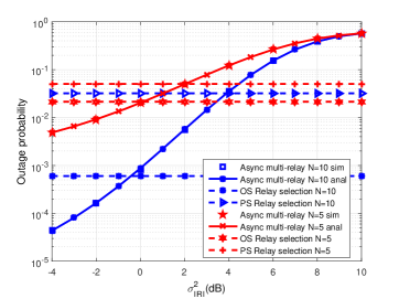
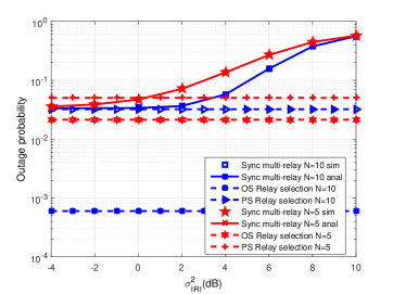
Figure 2: Outage probability versus the IRI of asynchronous case for $\sigma_{\mathit{\mathrm{SR}}}^{2}=8\,\mathrm{dB}$, $\sigma_{\mathrm{RD}}^{2}=10\,\mathrm{dB}$, $\sigma_{\mathrm{RSI}}^{2}=0\mathrm{\,dB}$, and $P_{\textrm{S}}=E_{\textrm{R}}=5\,\mathrm{dB}.$

Figure 3: Outage probability versus the IRI of synchronous case for $\sigma_{\mathrm{SR}}^{2}=8\mathrm{\,dB}$, $\sigma_{\mathrm{RD}}^{2}=10\,\mathrm{dB}$, $\sigma_{\mathrm{RSI}}^{2}=0\mathrm{\,dB}$, and $P_{\textrm{S}}=E_{\textrm{R}}=5\,\mathrm{dB}.$

Now, we focus on the asynchronous scenario and evaluate the outage probability of the studied system versus $\sigma_{\mathrm{SR}}^{2}$. In Fig. 4, we consider the scenario of a strong $\mathrm{R_{\mathit{k}}}\rightarrow\mathrm{D}$ link, i.e., $\sigma_{\mathrm{RD}}^{2}=10\,\mathrm{dB}$, and we can see clearly that the proposed multi-relay system and the OS scheme offer the same performances, while outperforming the PS scheme with the increase of $\sigma_{\mathrm{SR}}^{2}$. In Fig. 5, as the $\mathrm{R_{\mathit{k}}}\rightarrow\mathrm{D}$ link quality decreases, i.e., $\sigma_{\mathrm{RD}}^{2}=0\,\mathrm{dB}$, we start to notice that the OS scheme, provides better performances than the multi-relay system when $\sigma_{\mathrm{SR}}^{2}\geq 4\mathrm{\,dB}$. This is due to the fact that, in OS scheme, the relaying transmit power $E_{\mathrm{R}}$ is fully used by the best $\mathrm{R_{\mathit{k}}}\rightarrow\mathrm{D}$ link while, in multi-relay scheme, the relaying transmit power $E_{\mathrm{R}}$ is shared equally between $L$ relay links, i.e., $P_{\mathrm{R}}=\frac{E_{\mathrm{R}}}{L}$. Even though, the proposed scheme still performs better than the PS scheme.

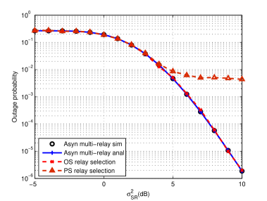
Figure 4: Asynchronous outage probability versus $\sigma_{\mathrm{SR}}^{2}$ for $N=10$, $\sigma_{\mathrm{RD}}^{2}=10\,\mathrm{dB}$, $\sigma_{\mathrm{RSI}}^{2}=\sigma_{\mathrm{IRI}}^{2}=0\mathrm{\,dB}$, and $P_{\textrm{S}}=E_{\textrm{R}}=10\,\mathrm{dB}.$

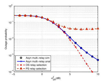
Figure 5: Asynchronous outage probability versus $\sigma_{\mathrm{SR}}^{2}$ for $N=10$, $\sigma_{\mathrm{RD}}^{2}=0\mathrm{\,dB}$, $\sigma_{\mathrm{RSI}}^{2}=\sigma_{\mathrm{IRI}}^{2}=0\mathrm{\,dB}$ and $P_{\textrm{S}}=E_{\textrm{R}}=10\,\mathrm{dB}.$

V Conclusion

In this paper, we proposed a low latency cooperative transmission scheme, where multiple FD-SDF relays, simultaneously, assist the communication between a source node and a destination node. First, the analytical expression of the outage probability were derived for two cases, i.e., asynchronous and synchronous transmissions. Then, using Monte-carlo simulations, we compared the proposed multi-relays transmission scheme with two different relay selection schemes, i.e., the OS scheme requiring the knowledge of global CSI and the PS scheme requiring the knowledge of partial CSI. Simulation results reveal that the proposed multi-relay transmission scheme and relay selection schemes outperform each other in term of outage probability, depending on IRI, number of relays, and channel links quality. As the proposed multiple FD cooperative relaying scheme does not require any central component, thus, getting rid of relay selection signaling messages and thereby, reducing the system latency while increasing the system diversity, we can say that it can be considered as a good candidate for very low latency applications.

References

[1]R. Abreu, P. Mogensen, and K. I. Pedersen, “Pre-scheduled
resources for retransmissions in ultra-reliable and low latency communications”,
in Proc. IEEE WCNC, San Francisco, USA, March 2017.
[2]H. Shariatmadari, S. Iraji, Z. Li, M. A. Uusitalo, and
R. Jäntti, “Optimized transmission and resource allocation strategies
for ultra-reliable communications”, in Proc. IEEE PIMRC,
Valencia, Spain, September 2016.
[3]J. Han, J. Baek, S. Jeon, and J. Seo, “Cooperative networks
with amplify-and-forward multiple-full-duplex relays”, IEEE
Transactions on Wireless Communications, Vol. 13, no. 4, pp. 2137
- 2149, April 2014.
[4]A. F. M. Shahen Shah and Md. Shariful Islam, “A survey
on cooperative communication in wireless networks”, I.J.
Intelligent Systems and Applications, pp. 66-78, June 2014.
[5]J. N. Laneman, D. Tse, and G. W. Wornell, “Cooperative
diversity in wireless networks: Efficient protocols and outage behavior”,
IEEE Trans. Inform. Theory, vol. 50, no. 12, pp. 3062-3080,
December. 2004.
[6]F. Atay Onat, H. Yanikomeroglu, and S. Periyalwar,
“Relay-assisted spatial multiplexing in wireless fixed relay networks”,
IEEE GLOBECOM, San Francisco, USA, Nov.- Dec. 2006.
[7]T. Riihonen, S. Werner, R. Wichman, and E. Zacarias, "On
the feasibility of full-duplex relaying in the presence of loop interference",
in Proc. IEEE SPAWC, Perugia, Italy, June 2009.
[8]T. Riihonen, S. Werner, and R. Wichman, “Optimized
gain control for single-frequency relaying with loop interference”,
IEEE Trans Wireless Commun, vol. 8, no. 6, pp. 2801–2806,
June 2009.
[9]J. I. Choi, M. Jain, K. Srinivasan, P. Levis, and S. Katti,
“Achieving single channel, full duplex wireless communication,”
in Proc. ACM MobiCom, Chicago, Illinois, USA, September
2010.
[10]M. Duarte, C. Dick, and A. Sabharwal, “Experiment-driven
characterization of full-duplex wireless systems,” IEEE
Transactions on Wireless Communications, vol. 11, no. 12, pp. 4296-4307,
May 2012.
[11]I. Krikidis, H. A. Suraweera, P. J. Smith, and C. Yuen,
“Full-duplex relay selection for amplify-and-forward cooperative
networks”, IEEE Transactions on Wireless Communications,
vol. 11, no. 12, pp. 4381-4393, December 2012.
[12]Y. Wang, Y. Xu, N. Li, W. Xie, K. Xu, and X. Xia, “Relay
selection of full-duplex decode-and-forward relaying over Nakagami-m
fading channels”, IET Communications, vol. 10, no. 12,
pp. 170-179, 2016.
[13]S. S. Ikki and M. H. Ahmed, “Performance analysis of
adaptive decode-and-forward cooperative diversity networks with best-relay
selection”, IEEE Transactions on Communications, vol. 58,
no. 1, January 2010.
[14]Z. Ding, I. Krikidis, B. Sharif, and H. V. Poor, “Wireless
information and power transfer in cooperative networks with spatially
random relays”, IEEE Transactions on Wireless Communications,
vol. 13, no. 8, pp. 4440-4453, 2014.
[15]A. Bletsas, A. Khisti, D. P. Reed, and A. Lippman, “A
simple cooperative diversity method based on network path selection”,
IEEE Journal on Selected Areas in Communications, vol. 24,
no. 3, pp. 659-672, March 2006.
[16]N. C. Beaulieu and J. Hu, “ A closed-form expression
for the outage probability of decode-and-forward relaying in dissimilar
Rayleigh fading channels”, IEEE Communications Letters,
vol. 10, no. 12, 2006.
[17]M. Jain, J. Choi, T. Kim, D. Bharadia, S. Seth, K. Srinivasan,
P. Levis, S. Katti, and, P. Sinha, “Practical, real-time,
full duplex wireless”, in Proc. ACMMobiCom,
Las Vegas, Nevada, USA, September 2011.
[18]H. Chafnaji, T. Ait-Idir, H. Yanikomeroglu, and S.
Saoudi, “Turbo packet combining for relaying schemes over multiantenna
broadband channels”, IEEE Transactions on Vehicular Technology,
vol. 61, no. 7, pp. 2965-2977, 2012.
[19]M. G. Khafagy, A. Ismail, M. S. Alouini, and S. Aïssa,
“On the outage performance of full-duplex selective decode-and-forward
relaying,” IEEE Communications Letters, vol. 17, no. 6,
pp. 1180-1183, April 2013.
[20]I. Gradshteyn and I. Ryzhik,“Table of Integrals,
Series and Products”, edition. London:
Academic Press, 2007.