Field theoretical derivation of Lüscher’s formula and calculation of finite volume form factors

Abstract

We initiate a systematic method to calculate both the finite volume energy levels and form factors from the momentum space finite volume two-point function. By expanding the two point function in the volume we extracted the leading exponential volume correction both to the energy of a moving particle state and to the simplest non-diagonal form factor. The form factor corrections are given in terms of a regularized infinite volume 3-particle form factor and terms related to the Lüsher correction of the momentum quantization. We tested these results against second order Lagrangian and Hamiltonian perturbation theory in the sinh-Gordon theory and we obtained perfect agreement.

1 Introduction

Quantum Field Theories play an important role in many branches of physics. On the one hand, they provide the language in which we formulate the fundamental interactions of Nature including the electro-weak and strong interactions. On the other hand, they are frequently used in effective models appearing in particle, solid state or statistical physics. In most of these applications the physical system has a finite size: scattering experiments are performed in a finite accelerator/detector, solid state systems are analyzed in laboratories, even the lattice simulations of gauge theories are performed on finite lattices etc. The understanding of finite size effects are therefore unavoidable and the ultimate goal is to solve QFTs for any finite volume. Fortunately, finite size corrections can be formulated purely in terms of the infinite volume characteristics of the theory, such as the masses and scattering matrices of the constituent particles and the form factors of local operators Luscher ; Luscher:1986pf ; Pozsgay:2007kn ; Pozsgay:2007gx . For a system in a box of finite sizes the leading volume corrections are polynomial in the inverse of these sizes and are related to the quantization of the momenta of the particles Luscher:1986pf . In massive theories the subleading corrections are exponentially suppressed and are due to virtual processes in which virtual particles “travel around the world” Luscher .

The typical observables of an infinite volume QFT (with massive excitations) are the mass spectrum, the scattering matrix, the matrix elements of local operators, i.e. the form factors, and the correlation functions of these operators. The mass spectrum and the scattering matrix is the simplest information, which characterize the QFT on the mass-shell. The form factors are half on-shell half off-shell data, while the correlation functions are completely off-shell information. These can be seen from the Lehmann-Symanzik-Zimmermann (LSZ) reduction formula, which connects the scattering matrix and form factors to correlation functions: The scattering matrix is the amputated momentum space correlation function on the mass-shell, while for form factors only the momenta, which correspond to the asymptotic states are put on shell. Clearly, correlation functions are the most general objects as form factors and scattering matrices can be obtained from them by restriction. Alternatively, however, the knowledge of the spectrum and form factors provides a systematic expansion of the correlation functions as well.

The field of two dimensional integrable models is an adequate testing ground for finite size effects. These theories are not only relevant as toy models, but, in many cases, describe highly anisotropic solid state systems and via the AdS/CFT correspondence, solve four dimensional gauge theories Mussardo:2010mgq ; Samaj:2013yva ; Beisert:2010jr . Additionally, they can be solved exactly and the structure of the solution provides valuable insight for higher dimensional theories. For simplicity we restrict our attention in this paper to a theory with a single massive particle, which does not form any boundstate.

The finite size energy spectrum has been systematically calculated in integrable theories. The leading finite size correction is polynomial in the inverse of the volume and originates from momentum quantization Luscher:1986pf . The finite volume wave-function of a particle has to be periodic, thus when moving the particle around the volume, $L$, it has to pick up the $pL$ translational phase. If the theory were free this phase should be $2\pi n$, in an interacting theory, however, the particle scatters on all the other particles suffering phase shifts, $-i\log S$, which adds to the translational phase and corrects the free quantization condition. These equations are called the Bethe-Yang (BY) equations. The energy of a multiparticle state is simply the sum of infinite volume energies but with the quantized momenta depending on the infinite volume scattering matrix. The exponentially small corrections are related to virtual processes. In the leading process a virtual particle anti-particle pair appears from the vacuum, one of them travels around the world, scatters on the physical particles and annihilates with its pair. Similar process modifies the large volume momentum quantization of the particles BaJa . The total energy contains not only the particles’ energies, but also the contribution of the sea of virtual particles. The next exponential correction contains two virtual particle pairs and a single pair which wraps twice around the cylinder Bombardelli:2013yka . For an exact description all of these virtual processes have to be summed up, which is provided by the Thermodynamic Bethe Ansatz (TBA) equations Zamolodchikov:1989cf . TBA equations can be derived (only for the ground state) by evaluating the Euclidean torus partition function in the limit, when one of the sizes goes to infinity. If this size is interpreted as Euclidean time, then only the lowest energy state, namely the finite volume ground state contributes. If, however, it is interpreted as a very large volume, then the partition function is dominated by the contribution of finite density states. Since the volume eventually goes to infinity the BY equations are almost exact and can be used to derive (nonlinear) TBA integral equations to determine the density of the particles, which minimize the partition function in the saddle point approximation. By careful analytical continuations this exact TBA integral equation can be extended for excited states Dorey:1996re .

The similar program to determine the finite volume matrix elements of local operators, i.e. form factors, is still in its infancy. Since there is a sharp difference between diagonal and non-diagonal form factors they have to be analyzed separately. For nondiagonal form factors the polynomial finite size corrections, besides the already explained momentum quantization, involve also the renormalization of states, to conform with the finite volume Kronecker delta normalization Pozsgay:2007kn . The polynomial corrections for diagonal form factors are much more complicated, as they contain disconnected terms. They were conjectured in Saleur:1999hq ; Pozsgay:2007gx and confirmed in Bajnok:2017bfg . For exponential corrections the situation is the opposite. Exact expressions for the finite volume one-point function can be obtained in terms of the TBA minimizing particle density and the infinite volume form factors by evaluating the one-point function on an Euclidean torus where one of the sizes is sent to infinity Leclair:1999ys . The analytical continuation trick used for the spectrum can be generalized and leads to exact expressions for all finite volume diagonal form factors Pozsgay:2013jua . For non-diagonal form factors, however, not even the leading exponential correction is known for theories without boundstates. In case of boundstates the leading exponential volume correction is in fact the so called $\mu$ term, which originates from a process in which the particle can virtually decay in a finite volume into its constituents. This idea was used to calculate the leading $\mu$ term explicitly for the simplest non-diagonal form factor in Pozsgay:2008bf . As we would like to calculate the leading volume correction coming from virtual particles travelling around the world, i.e. the F-term, we focus on theories without boundstates. The aim of this paper is to initiate research into the calculation of these corrections.

We develop a framework which provides direct access both to excited states’ energy levels and finite volume form factors. The idea is to calculate the Euclidean torus two-point function in the limit, when one of the sizes is sent to infinity. The exact finite volume two-point function then can be used, similarly to the LSZ formula, to extract the information needed: the momentum space two-point function, when continued analytically to imaginary values, has poles exactly at the finite volume energy levels whose residues are the products of finite volume form factors. Of course, the exact determination of the finite-volume two-point function is hopeless in interacting theories, but developing any systematic expansion leads to a systematic expansion of both the energy levels and the form factors. We analyze two such expansions in this paper: in the first, we expand the two-point function in the volume, which leads to the leading exponential corrections. We perform the calculation for a moving one-particle state. In the second expansion, we calculate the same quantities perturbatively in the coupling in the sinh-Gordon theory. By comparing the two approaches in the overlapping domain we find complete agreement.

The paper is organized as follows: In the next section we give an overview of the method and present our main result for the leading exponential volume correction of the simplest nondiagonal form factor. In section 3 we present the details of the calculation in the mirror channel and derive the correction explicitly. In section 4 we specify the results for the sinh-Gordon theory in preparation for a perturbative check. We use Hamiltonian perturbation theory in section 5 to derive the leading finite size correction in the coupling both to the one-particle energy and form factor. Technical details are relegated to Appendix B. We then expand these results in the volume and confirm the previously derived leading exponential finite size corrections. Finally, we finish the main body of the paper with conclusions in section 6. We have several Appendices. Appendix A contains the perturbative expansion of the exact TBA equations. In Appendix C we make a perturbative expansion of the finite volume two point function in the sinh-Gordon theory and extract the leading correction to the finite volume energy and form factors confirming the results of section 4. Appendix D shows the equivalence of the finite volume regularizations of Pozsgay:2010cr with our infinite volume regularizations.

2 Overview of the method and summary of the results

In the following we analyze a relativistic integrable QFT in two dimensions with a single particle of mass $m$ and scattering matrix $S(\theta)$, which satisfies unitarity and crossing symmetry $S(\theta)=S(-\theta)^{-1}=S(i\pi-\theta)$ and does not have any pole in the physical strip. Such theory is the sinh-Gordon theory and the generalization for more species with diagonal scatterings is straightforward. We put this QFT in a finite volume of size $L$ and focus on the finite size energy spectrum and the finite size form factors.

2.1 Finite size energy spectrum

We analyze the energy of an $N$ particle state with rapidities $\theta_{k}$, $k=1,\dots,N$. As explained in the introduction the polynomial corrections come from the quantization of momenta formulated by the Bethe-Yang equations

$$\epsilon^{(0)}(\theta_{j}^{(0)}+i\frac{\pi}{2})=i(2n_{j}+1)\pi\quad;\qquad\epsilon^{(0)}(\theta+i\frac{\pi}{2})=imL\sinh\theta+\sum_{k}\log S(\theta-\theta_{k}^{(0)})$$ (2.1)

where, by the superscript $(0)$, we indicated that only the polynomial volume corrections are kept. Given integers $n_{1},\dots,n_{N}$ the rapidities $\theta_{1}^{(0)},\dots,\theta_{N}^{(0)}$ can be determined leading to the energy formula

$$E_{N}(L)=\sum_{i}m\cosh\theta_{i}^{(0)}+O(e^{-mL})$$ (2.2)

The leading exponential correction was conjectured in BaJa and has two sources. First one has to take into account how the sea of virtual particles changes the quantization condition

$$\epsilon^{(1)}(\theta_{j}^{(1)}+i\frac{\pi}{2})=i(2n_{j}+1)\pi\quad;\qquad\epsilon^{(1)}(\theta)=\epsilon^{(0)}(\theta)+\delta\epsilon(\theta)\,\,\,\,\,\,\,\,\,\,\,\,\,\,\,\,\,\,\,\,\,\,\,\,\,$$

$$\delta\epsilon(\theta)=i\int_{-\infty}^{\infty}\frac{d\theta^{{}^{\prime}}}{2\pi}\frac{S^{\prime}(\theta-\theta^{{}^{\prime}})}{S(\theta-\theta^{{}^{\prime}})}\prod_{k}S(i\frac{\pi}{2}+\theta_{k}^{(0)}-\theta^{{}^{\prime}})e^{-mL\cosh\theta^{{}^{\prime}}}$$ (2.3)

where $S^{\prime}(\theta)$ denotes $\frac{dS(\theta)}{d\theta}$. We then have to add the direct energy contribution of the virtual particles. By expressing all contributions in terms of the leading rapidities, $\theta_{j}^{(0)}$, we have:

$$E_{N}(L) = \sum_{k}m\cosh\theta_{k}^{(0)}+i\sum_{k,j}m\sinh\theta_{k}^{(0)}\left(\bar{\rho}_{N}^{(0)}\right)^{kj}\delta\epsilon(\theta_{j}^{(0)}+i\frac{\pi}{2})$$ (2.4)

$$-m\int_{-\infty}^{\infty}\frac{d\theta}{2\pi}\,\cosh\theta\,\prod_{k}S(\frac{i\pi}{2}+\theta-\theta_{k}^{(0)})e^{-mL\cosh\theta}$$

where $\bar{\rho}_{N}^{(0)}$ is the inverse of the matrix $\rho_{N}^{(0)}$ with entries $\rho_{jk}^{(0)}=-i\partial_{\theta_{j}^{(0)}}\epsilon^{(0)}(\theta_{k}^{(0)}+i\frac{\pi}{2})$.

The exact equations come either from an analytical continuation of the groundstate TBA result Dorey:1996re ; Bajnok:2010ke or from a continuum limit of a solved integrable lattice regularization Teschner:2007ng . The quantization condition for the exact rapidities $\theta_{j}$ is

$$\epsilon(\theta_{j}+i\frac{\pi}{2})=i(2n_{j}+1)\pi$$ (2.5)

where $\epsilon$ satisfies the coupled non-linear integral equation

$$\epsilon(\theta)=mL\cosh\theta+\sum_{j}\log S(\theta-\theta_{j}-\frac{i\pi}{2})+i\int_{-\infty}^{\infty}\frac{d\theta^{{}^{\prime}}}{2\pi}\frac{S^{\prime}(\theta-\theta^{{}^{\prime}})}{S(\theta-\theta^{{}^{\prime}})}\log(1+e^{-\epsilon(\theta^{{}^{\prime}})})$$ (2.6)

and the energy is

$$E_{N}(L)=m\sum_{i}\cosh\theta_{i}-m\int_{-\infty}^{\infty}\frac{d\theta}{2\pi}\,\cosh\theta\,\log(1+e^{-\epsilon(\theta)})$$ (2.7)

In particular, for a moving one-particle state at leading order we obtain

$$-i\epsilon^{(0)}(\theta_{1}^{(0)}+i\frac{\pi}{2})=mL\sinh\theta_{1}^{(0)}+\pi=(2n_{1}+1)\pi$$ (2.8)

and the corresponding energy is

$$E_{1}(L)=m\cosh\theta_{1}^{(0)}+O(e^{-mL})$$ (2.9)

The leading exponential correction of the quantization condition contains an extra term of the form

$$\delta\epsilon\left(\theta_{1}^{(0)}+i\frac{\pi}{2}\right)=i\int_{-\infty}^{\infty}\frac{d\theta^{{}^{\prime}}}{2\pi}S^{\prime}(i\frac{\pi}{2}+\theta_{1}^{(0)}-\theta^{{}^{\prime}})e^{-mL\cosh\theta^{{}^{\prime}}}$$ (2.10)

The one-particle energy (measured from the finite volume vacuum) is KlMe ; JaLu :

$$E_{1}(L)-E_{0}(L) = m\cosh\theta_{1}^{(0)}-$$

$$\frac{m}{\cosh\theta_{1}^{(0)}}\int_{-\infty}^{\infty}\frac{d\theta}{2\pi}\,\cosh(\theta-\theta_{1}^{(0)})\,(S(\frac{i\pi}{2}+\theta-\theta_{1}^{(0)})-1)e^{-mL\cosh\theta}$$

We will reproduce this result from the study of the finite volume two-point function.

2.2 Finite size form factors

Form factors are defined as the matrix elements of local operators sandwiched between finite volume energy eigenstates. These states are normalized to Kronecker-$\delta$ functions

$$\langle n_{1}^{\prime},\dots,n_{M}^{\prime}|n_{1},\dots,n_{N}\rangle_{L}=\delta_{N,M}\prod_{j}\delta_{n_{j}^{\prime}n_{j}}$$ (2.12)

opposed to infinite volume states, which are normalized to Dirac-$\delta$ functions: $\langle\theta^{\prime}|\theta\rangle=\delta(\theta^{\prime}-\theta)$. The finite volume states can be equivalently labeled by the rapidities $|n_{1},\dots,n_{N}\rangle_{L}\equiv|\theta_{1},\dots,\theta_{N}\rangle_{L}$. The space-time dependence of the form factors can be easily calculated

$$\langle\theta_{1}^{\prime},\dots,\theta^{\prime}_{M}|\mathcal{O}(x,t)|\theta_{1},\dots,\theta_{N}\rangle_{L}=e^{i\Delta Et-i\Delta Px}\langle\theta_{1}^{\prime},\dots,\theta^{\prime}_{M}|\mathcal{O}|\theta_{1},\dots,\theta_{N}\rangle_{L}$$ (2.13)

where $\Delta E=E_{M}(L)-E_{N}(L)$ and $\Delta P=P_{M}(L)-P_{N}(L)$ with $P_{N}(L)=\frac{2\pi}{L}\sum_{j}n_{j}$, while we simply abbreviated $\mathcal{O}(0,0)$ by $\mathcal{O}$.

The polynomial finite size corrections purely change the normalization of states and give Pozsgay:2007kn :

$$\langle\theta_{1}^{\prime},\dots,\theta^{\prime}_{M}|\mathcal{O}|\theta_{1},\dots,\theta_{N}\rangle_{L}=\frac{F_{M+N}^{\mathcal{O}}(\theta_{1}^{\prime}+i\pi,\dots,\theta^{\prime}_{M}+i\pi,\theta_{1},\dots,\theta_{N})}{\sqrt{(2\pi)^{-N-M}\mbox{det}\rho_{M}^{(0)}\det\rho_{N}^{(0)}}}+O(e^{-mL})$$ (2.14)

where $F_{M+N}^{\mathcal{O}}$ denotes the infinite volume form factor

$$F_{M+N}^{\mathcal{O}}(\theta_{1}^{\prime},\dots,\theta^{\prime}_{M},\theta_{1},\dots,\theta_{N})=\langle 0|\mathcal{O}|\theta_{1}^{\prime},\dots,\theta^{\prime}_{M},\theta_{1},\dots,\theta_{N}\rangle$$ (2.15)

and all the rapidities can be taken at the leading order values with superscript $(0)$. Since even the leading exponential correction is not known for these form factors we develop a systematic method based on the two-point function to calculate them.

In particular, for the one-particle form factor the formulae simplify as

$$\langle 0|\mathcal{O}|\theta_{1}\rangle_{L}=\frac{F_{1}^{\mathcal{O}}(\theta_{1}^{(0)})}{\sqrt{\rho_{1}^{(0)}/(2\pi)}}+O(e^{-mL})$$ (2.16)

where

$$\rho_{1}^{(0)}=-i\partial_{\theta_{1}^{(0)}}\epsilon^{(0)}(\theta_{1}^{(0)}+i\frac{\pi}{2})=mL\cosh\theta_{1}^{(0)}$$ (2.17)

and the aim of our paper is to calculate the leading exponential corrections to these formulae.

2.3 Finite volume two-point function

Let us focus on the Euclidean finite volume two-point function, which is defined by the path integral

$$\langle\mathcal{O}(x,t)\mathcal{O}\rangle_{L}=\frac{\int[\mathcal{D}\phi]\mathcal{O}(x,t)\mathcal{O}(0,0)e^{-S[\phi]}}{\int[\mathcal{D}\phi]e^{-S[\phi]}}$$ (2.18)

where configurations are periodic in $x$ with $L$ and $t\in\mathbb{R}$. The momentum space form is obtained by its Fourier transform

$$\Gamma(\omega,q)=\frac{1}{L}\int_{-L/2}^{L/2}{\rm d}x\int_{-\infty}^{\infty}{\rm d}t\,{\rm e}^{i(\omega t+qx)}\langle\mathcal{O}(x,t)\mathcal{O}\rangle_{L}$$ (2.19)

where periodicity in $x$ requires that $e^{iqL}=1$. Taking $t$ as Euclidean time the two point function is the vacuum expection value of the time ordered product:

$$\langle\mathcal{O}(x,t)\mathcal{O}\rangle_{L}=\langle 0|T(\mathcal{O}(x,t)\mathcal{O})|0\rangle_{L}=\Theta(t)\langle 0|\mathcal{O}(x,t)\mathcal{O}|0\rangle_{L}+\Theta(-t)\langle 0|\mathcal{O}\mathcal{O}(x,t)|0\rangle_{L}$$ (2.20)

We can insert a complete system of finite volume energy-momentum eigenstates and use the Euclidean version of the space-time dependence (2.13). By performing the integrals we obtain

$$\Gamma(\omega,q)=\sum_{N}|\langle 0|\mathcal{O}|\theta_{1},\dots,\theta_{N}\rangle_{L}|^{2}\left\{\frac{\delta_{q-P_{N}(L)}}{E_{N}(L)-i\omega}+\frac{\delta_{q+P_{N}(L)}}{E_{N}(L)+i\omega}\right\}$$ (2.21)

For a fixed $q$ we can determine the energy levels by searching for poles in the analytically continued $\omega$. For a generic volume and fixed momentum $q$ the energy levels are never degenerate. Thus the poles are located at $\omega=\pm iE_{N}(L)$ with residue

$$\lim_{\omega\to\pm iE_{N}(L)}(E_{N}(L)\pm i\omega)\Gamma(\omega,\pm P_{N}(L))=|\langle 0|\mathcal{O}|\theta_{1},\dots,\theta_{N}\rangle_{L}|^{2}$$ (2.22)

which is nothing but the square of the finite volume form factor.

In order to obtain the exponential corrections of these form factors we have to expand the two point function on the space-time cylinder in $L$. The Euclidean version of this cylinder can be thought of as the large size limit of the torus. On the torus we can exchange the role of the Euclidean time and space and represent the two point function as

$$\langle\mathcal{O}(x,t)\mathcal{O}\rangle_{L}=\Theta(x)\frac{\mbox{Tr}[\mathcal{O}(0,t)e^{-Hx}\mathcal{O}e^{-H(L-x)}]}{\mbox{Tr}[e^{-HL}]}+\Theta(-x)\frac{\mbox{Tr}[\mathcal{O}e^{Hx}\mathcal{O}(0,t)e^{-H(L+x)}]}{\mbox{Tr}[e^{-HL}]}$$ (2.23)

Inserting two complete system of (mirror) states denoted by $|\mu\rangle$ and $|\nu\rangle$ and exploiting the $|\langle\nu|\mathcal{O}|\mu\rangle|=|\langle\mu|\mathcal{O}|\nu\rangle|$ symmetry together with $e^{iqL}=1$ we obtain:

$$Z\Gamma(\omega,q)=\frac{2\pi}{L}\sum_{\mu,\nu}|\langle\nu|\mathcal{O}|\mu\rangle|^{2}e^{-E_{\nu}L}\delta(P_{\mu}-P_{\nu}+\omega)\left\{\frac{1}{E_{\mu}-E_{\nu}-iq}+\frac{1}{E_{\mu}-E_{\nu}+iq}\right\}$$ (2.24)

where $Z=\mbox{Tr}[e^{-HL}]$. Note that the expansion in $\nu$ naturally corresponds to expansions in Lüscher orders. In the bulk of the paper we perform a systematic expansion related to a moving one-particle state. Let us summarize the result we got.

For a one-particle state we focus on the one-particle finite volume pole

$$\Gamma(\omega,q)=\frac{\mathcal{F}(q)^{2}}{E(q)+i\omega}+\dots\quad;\qquad\mathcal{F}(q)=\langle 0|\mathcal{O}|q\rangle$$ (2.25)

where $E(q)$ is the exact finite volume energy with momentum $q$ and $\mathcal{F}(q)$ is the corresponding exact finite volume form factor. We choose the phase of the one-particle state so that $\mathcal{F}(q)$ is real and positive. We used the momentum variable to label the state, which is related to the rapidity as $q=m\sinh\theta_{1}$, such that the corresponding energy is $\mathcal{E}(q)=m\cosh\theta_{1}$. We can expand $\Gamma$ around the large volume Bethe-Yang pole at $\omega=i\mathcal{E}(q)$. At the leading Lüscher order we have first and second order poles

$$\Gamma(\omega,q)=\frac{2\pi F_{1}^{2}}{L\mathcal{E}(q)}\frac{-i}{\omega-i\mathcal{E}(q)}+\frac{\mathcal{L}_{0}(q)}{(\omega-i\mathcal{E}(q))^{2}}+\frac{\mathcal{L}_{1}(q)}{\omega-i\mathcal{E}(q)}+\mathrm{regular}$$ (2.26)

such that the leading exponential corrections of the energy and form factor can be written as

$$E(q)=\mathcal{E}(q)\left\{1+\frac{L}{2\pi F_{1}^{2}}\mathcal{L}_{0}(q)+\dots\right\}\quad;\quad\mathcal{F}(q)=\frac{\sqrt{2\pi}F_{1}}{\sqrt{L\mathcal{E}(q)}}\left\{1+\frac{iL\mathcal{E}(q)}{4\pi F_{1}^{2}}\mathcal{L}_{1}(q)+\dots\right\}$$ (2.27)

We calculate $\Gamma$ in the mirror channel (2.24). The leading order result comes from terms, when $\langle\nu|$ is the vacuum state $\langle 0|$ and $|\mu\rangle$ is a one-particle state. The leading Lüscher corrections, $\mathcal{L}_{0}$ and $\mathcal{L}_{1}$, come from terms when $\langle\nu|$ is a one-particle state and $|\mu\rangle$ is either the vacuum or a two-particle state.

Having performed the calculations we could reproduce the Lüscher correction of the 1-particle energy (2.1). For the form factors we obtained the result

$$\mathcal{F}(q)=\frac{\sqrt{2\pi}}{\sqrt{\rho_{1}^{(1)}}}\left\{F_{1}+\int_{-\infty}^{\infty}d\theta\,F_{3}^{\mathrm{reg}}(\theta+i\pi,\theta,\theta_{1}^{(0)}-i\frac{\pi}{2})e^{-mL\cosh\theta}+\dots\right\}$$ (2.28)

where the density of states at the leading exponential order is

$$\rho_{1}^{(1)}=-i\partial_{\theta^{(1)}}\epsilon^{(1)}(\theta^{(1)}+i\frac{\pi}{2})$$ (2.29)

and the regularized form factor is defined to be

$$F_{3}^{\mathrm{reg}}(\theta,\theta_{1},\theta_{2})=F_{3}(\theta,\theta_{1},\theta_{2})-\frac{iF_{1}}{2\pi}\frac{1-S(\theta_{1}-\theta_{2})}{\theta-\theta_{1}-i\pi}+\frac{iF_{1}}{4\pi}S^{\prime}(\theta_{1}-\theta_{2})$$ (2.30)

In the rest of the paper we derive this result and check it by a second order perturbative calculation in the sinh-Gordon theory.

3 Mirror representation

We perform our calculation starting from the mirror representation (2.24). The denominator has the Hilbert space representation

$$Z=\sum_{\nu}\langle\nu|\nu\rangle{\rm e}^{-E_{\nu}L}$$ (3.1)

and we see that its Lüscher expansion,

$$Z=1+\delta(0)\int{\rm d}u\,{\rm e}^{-mL\cosh u}+\dots$$ (3.2)

is divergent. The divergent constant $\delta(0)$ comes from the continuum normalization. As we will see, this divergence cancels with a similar term from the numerator. However, we need some regularization to make intermediate steps well-defined. In the main text we will use continuum regularization, but as shown in Appendix D, this is completely equivalent to finite volume regularization.

The leading (0th order) term in the Lüscher expansion of $\Gamma(\omega,q)$ is

$$\frac{4\pi}{L}\sum_{\mu}|\langle 0|{\cal O}|\mu\rangle|^{2}\frac{E_{\mu}\,\delta(P_{\mu}+\omega)}{E_{\mu}^{2}+q^{2}}.$$ (3.3)

It is easy to see that this is regular in $\omega$ (around the 1-particle pole) unless $|\mu\rangle$ is a 1-particle state. Indeed, the $n$-particle contribution can be written as

$$\frac{4\pi}{L}\int_{-\infty}^{\infty}{\rm d}\beta_{1}\int_{-\infty}^{\beta_{1}}{\rm d}\beta_{2}\,\cdots\int_{-\infty}^{\beta_{n-1}}{\rm d}\beta_{n}\left|\langle 0|{\cal O}|\beta_{1},\dots\beta_{n}\rangle\right|^{2}\frac{E_{n}(\beta)\delta(P_{n}(\beta)+\omega)}{E_{n}^{2}(\beta)+q^{2}}.$$ (3.4)

After changing the integration variables to the relative rapidities $u_{i}=\beta_{i}-\beta_{1}$, $i=2,\dots,n$ and the global rapidity $\lambda=(\sum_{i=1}^{n}\beta_{i})/n$ this becomes:

$$\frac{4\pi}{L}\int_{-\infty}^{\infty}{\rm d}\lambda\int({\cal D}u)_{n}|F_{n}(u)|^{2}\,\frac{{\cal M}_{n}(u)\cosh\lambda\,\delta({\cal M}_{n}(u)\sinh\lambda+\omega)}{{\cal M}_{n}^{2}(u)\cosh^{2}\lambda+q^{2}},$$ (3.5)

where the matrix element ($n$-particle form factor $F_{n}$) only depends on the relative rapidities and ${\cal M}_{n}(u)$ is the $n$-particle invariant mass. Performing the $\lambda$ integral with the help of the delta function we get

$$\frac{4\pi}{L}\int({\cal D}u)_{n}|F_{n}(u)|^{2}\,\frac{1}{{\cal M}_{n}^{2}(u)+\omega^{2}+q^{2}}.$$ (3.6)

Since ${\cal M}_{n}(u)\geq nm$ there is a singularity at $\omega^{2}+q^{2}=-m^{2}$ only for $n=1$.

Similarly, the first Lüscher correction in (2.24) (i.e. terms where $|\nu\rangle$ is a one-particle state) is regular unless $|\mu\rangle$ is the vacuum or a 2-particle state. As we will see, the $n$-particle contribution can be evaluated (after regularization) by shifting the integration contour for the rapidity integration away from the real axis. Performing the $\beta_{1}$ integration first, we notice that the matrix element (form factor)

$$\langle u|{\cal O}|\beta_{1},\dots,\beta_{n}\rangle$$ (3.7)

has a pole singularity in the variable $\beta_{1}$ at $\beta_{1}=u$ and so the total contribution consists of a residue term plus a shifted integral. As we will see, the shifted integral is not singular in $\omega$ at the 1-particle pole, while the residue term is proportional to

$$\int_{-\infty}^{\infty}{\rm d}\lambda\frac{\delta({\cal M}_{n-1}(u)\sinh\lambda+\omega)}{{\cal M}_{n-1}(u)\cosh\lambda-iq},$$ (3.8)

where $\lambda$ is the global rapidity of the remaining $(n-1)$-particle system, $\lambda=(\sum_{i=2}^{n}\beta_{i})/(n-1)$, ${\cal M}_{n-1}(u)$ is the invariant mass of this remaining system and $u_{i}=\beta_{i}-\beta_{2}$, $i=3,\dots,n$. After performing the $\lambda$ integral, the denominator

$${\cal M}_{n-1}^{2}(u)+\omega^{2}+q^{2}$$ (3.9)

leads to pole singularities only for $n=2$.

The (potentially) singular part of the first Lüscher correction to the 2-point function is of the form

$${\cal L}^{\rm sing}(\omega,q)=\frac{2\pi}{m^{2}L}\int_{\cosh u<2}{\rm d}u\,{\rm e}^{-mL\cosh u}\big{[}J(u,\psi,q)+J(u,\psi,-q)\big{]},$$ (3.10)

where

$$J(u,\psi,q)=-\delta(0)F_{1}^{2}\frac{1}{\cosh\psi(\cosh\psi-i\hat{q})}-F_{1}^{2}\delta(u-\psi)\frac{1}{\cosh\psi(\cosh\psi-i\hat{q})}+j(u,\psi,q)$$ (3.11)

and

$$j(u,\psi,q)=\int_{-\infty}^{\infty}{\rm d}\beta_{1}\int_{-\infty}^{\beta_{1}}{\rm d}\beta_{2}|\langle u|{\cal O}|\beta_{1},\beta_{2}\rangle|^{2}\frac{\delta(\sinh\beta_{1}+\sinh\beta_{2}-\sinh u-\sinh\psi)}{\cosh\beta_{1}+\cosh\beta_{2}-\cosh u-i\hat{q}}.$$ (3.12)

Here we introduced the notations

$$q=m\hat{q},\qquad\qquad\omega=-m\sinh\psi.$$ (3.13)

The first term in (3.11) comes from the combination of the 1-particle contribution to the $0$th order correlation function with the first order term, proportional to $\delta(0)$, coming from the denominator in (2.24) (see (3.6) and (3.2)). The second term comes from (2.24) when $|\mu\rangle$ is the vacuum state and finally the third term is the 2-particle contribution when $|\mu\rangle=|\beta_{1},\beta_{2}\rangle$. Note that we restricted the $u$ integration to the range $\cosh u<2$. This is possible since for $\cosh u>2$ the contribution is subleading to the second Lüscher order, which is O$({\rm e}^{-2mL})$ and which we neglect. This restriction is also necessary for some of our later estimates to be valid.

The matrix element $\langle u|{\cal O}|\beta_{1},\beta_{2}\rangle$ can be represented in terms of the S-matrix $S(\theta)$ and the 3-particle form factor $F_{3}(u,\beta_{1},\beta_{2})$ as Smirnov:1992vz

$$\langle u|{\cal O}|\beta_{1},\beta_{2}\rangle=\delta(u-\beta_{1})F_{1}+S(\beta_{1}-\beta_{2})\delta(u-\beta_{2})F_{1}+F_{3}(u+i\pi-i\epsilon,\beta_{1},\beta_{2}).$$ (3.14)

The integral of its square is divergent and needs to be regularized.

3.1 Regularization

We will use the regularized delta function

$$\delta(x)\rightarrow\frac{i}{2\pi}\left(\frac{1}{x+i\epsilon}-\frac{1}{x-i\epsilon}\right)$$ (3.15)

in (3.14) and take the limit $\epsilon\to 0$ only at the end of the calculation.

The regularized delta function terms can be nicely combined with those coming from the pole terms in the 3-particle form factor and the regularized matrix element becomes

$$\begin{split}\langle u|{\cal O}|\beta_{1},\beta_{2}\rangle^{\rm reg}=\frac{iF_{1}}{2\pi}&\left[\frac{1}{u-\beta_{1}+i\epsilon}-\frac{S(\beta_{1}-\beta_{2})}{u-\beta_{1}-i\epsilon}+\frac{S(\beta_{1}-\beta_{2})}{u-\beta_{2}+i\epsilon}-\frac{1}{u-\beta_{2}-i\epsilon}\right]\\ &+F_{3}^{c}(u+i\pi-i\epsilon,\beta_{1},\beta_{2}).\end{split}$$ (3.16)

Here $F_{3}^{c}$ is the finite part of the form factor, defined by

$$F_{3}(u,\beta_{1},\beta_{2}) =F_{3}^{c}(u,\beta_{1},\beta_{2})+\frac{iF_{1}}{2\pi(u-\beta_{1}-i\pi)}[1-S(\beta_{1}-\beta_{2})]$$ (3.17)

$$+\frac{iF_{1}}{2\pi(u-\beta_{2}-i\pi)}[S(\beta_{1}-\beta_{2})-1].$$ (3.18)

The finite part is obtained by explicitly removing the pole singularities required by the form factor axioms Smirnov:1992vz . $F_{3}^{c}(u,\beta_{1},\beta_{2})$ is finite at $u=\beta_{1}+i\pi$, $u=\beta_{2}+i\pi$. For later use, we now also define the modified form factor $\hat{F}_{3}$:

$$F_{3}(u,\beta_{1},\beta_{2})=\frac{iF_{1}}{2\pi(u-\beta_{1}-i\pi)}[1-S(\beta_{1}-\beta_{2})]+\hat{F}_{3}(u,\beta_{1},\beta_{2}).$$ (3.19)

$F_{3}^{\rm reg}$, defined by (2.30), can be written as

$$F_{3}^{\rm reg}(u,\beta_{1},\beta_{2})=\hat{F}_{3}(u,\beta_{1},\beta_{2})+\frac{iF_{1}}{4\pi}\,S^{\prime}(\beta_{1}-\beta_{2}).$$ (3.20)

Next we introduce the variables $b$, $w$ by

$$\beta_{1}=b+w,\qquad\qquad\beta_{2}=b-w$$ (3.21)

and integrate (3.12) over $b$ using the delta function. This means that after this integration $b$ stands for the solution of

$$\sinh b=\frac{\sinh u+\sinh\psi}{2\cosh w}.$$ (3.22)

We have

$$j(u,\psi,q)=\int_{-\infty}^{\infty}{\rm d}w|\langle u|{\cal O}|b+w,b-w\rangle^{\rm reg}|^{2}\frac{1}{C(C-\cosh u-i\hat{q})},$$ (3.23)

where

$$C=\cosh(b+w)+\cosh(b-w).$$ (3.24)

Next we make use of the analyticity of the form factors and shift the $w$ integral from real $w$ to $w=v+i\gamma$, where $\gamma>0$ is small. We have to pay attention to the following.

• The right hand side of (3.22) must not cross the cut of the arcsinh function (which runs from $i$ to $i\infty$ along the imaginary axis).

• Avoid points where $C=\cosh u+i\hat{q}$.

• Take into account the poles of the regularized matrix elements at $w=\pm(u-b\pm i\epsilon)$.

Problems A) and B) can be easily avoided if $\cosh u<2$ and the parameter $\gamma$ is small enough. The form factor poles can be taken into account explicitly, using the residue theorem. (Only two of the poles lie above the real axis.) After a long computation, we find (up to terms vanishing in the $\epsilon\to 0$ limit):

$$\begin{split}J(u,\psi,q)=&\left(\frac{F_{1}^{2}}{2\pi\epsilon}-\delta(0)F_{1}^{2}\right)\frac{1}{\cosh\psi(\cosh\psi-i\hat{q})}+I(u,\psi,q)\\ &+\frac{F_{1}}{\cosh\psi(\cosh\psi-i\hat{q})}[F_{3}^{c}(u+i\pi,u,\psi)+F_{3}^{c}(u+i\pi,\psi,u)]\\ &+\frac{iF_{1}^{2}}{4\pi}\frac{\sinh(u-\psi)[S(\psi-u)-S(u-\psi)]}{\cosh^{2}\psi(\cosh\psi-i\hat{q})^{2}}\\ &+\frac{iF_{1}^{2}}{4\pi}\frac{1}{\cosh\psi(\cosh\psi-i\hat{q})}\Big{[}\frac{2[S(u-\psi)-S(\psi-u)]}{u-\psi}+\frac{\nu[S^{\prime}(\psi-u)+S^{\prime}(u-\psi)]}{\cosh\psi}\\ &+\frac{\sinh(u-\psi)[S(\psi-u)-S(u-\psi)]}{\nu\cosh\psi}\\ &+\frac{(\sinh\psi+\sinh u)(1+\sinh u\sinh\psi)[S(u-\psi)-S(\psi-u)]}{\nu\cosh^{2}\psi}\Big{]}.\end{split}$$ (3.25)

Here the notation

$$\nu=\cosh\psi+\cosh u$$ (3.26)

is used and $I(u,\psi,q)$ is the shifted integral ($w=v+i\gamma$):

$$I(u,\psi,q)= \int_{-\infty}^{\infty}\frac{{\rm d}v}{C(C-\cosh u-i\hat{q})}S(-2w)\bigg{\{}\frac{iF_{1}}{2\pi}\left[\frac{1-S(2w)}{u-b-w}+\frac{S(2w)-1}{u-b+w}\right]$$ (3.27)

$$+F_{3}^{c}(u+i\pi-b,w,-w)\bigg{\}}^{2}.$$ (3.28)

The (negative) divergent term coming from the denominator is accompanied with a (positive) divergent term coming from the calculation of the numerator. They both multiply the same function. Our main assumption is that the divergences cancel and the remaining finite terms are correct. Indeed, in appendix D we show that our heuristic regularization is completely equivalent to the well-defined finite volume regularization. We will make the substitution

$$\left(\frac{1}{2\pi\epsilon}-\delta(0)\right)\rightarrow\Delta,$$ (3.29)

where $\Delta$ is a finite renormalization constant, which will be fixed later.

3.2 Analytic continuation

(3.25) is our final result for the Fourier space 2-point function for real $\omega$. We need to analytically continue this function towards $\omega\to i{\cal E}(q)$. We will do it in two steps. First we extend it to a small region where $\omega$ is just above the real axis. The explicit terms are analytic, so we have to concentrate on the integral $I(u,\psi,q)$. In this region there is no problem with A) and B), but as we increase the imaginary part of $\omega$, the integration contour will cross the double pole at $w=(u-\psi)/2$ coming from the form factor function squared. We can take into account the effects of this pole explicitly, using the residue theorem. After a second long calculation, we find that adding these new contributions to (3.25) many terms cancel and we have

$$\begin{split}J(u,\psi,q)&=I_{0}(u,\psi,q)+\frac{iF_{1}^{2}}{2\pi}\frac{\sinh(u-\psi)[1-S(u-\psi)]}{\cosh^{2}\psi(\cosh\psi-i\hat{q})^{2}}\\ &+\frac{1}{\cosh\psi(\cosh\psi-i\hat{q})}\Big{\{}F_{1}^{2}\Delta+2F_{1}\hat{F}_{3}(u+i\pi,u,\psi)+\\ &\frac{iF_{1}^{2}}{2\pi}\Big{[}\frac{\nu S^{\prime}(u-\psi)}{\cosh\psi}+\frac{\sinh\psi\cosh u}{\cosh^{2}\psi}[S(u-\psi)-1]\Big{]}\Big{\}},\end{split}$$ (3.30)

where $I_{0}(u,\psi,q)$ is the same integral as (3.28), but with the $w$ integration contour moved back to the real axis. (We are allowed to do this after $\omega$ is already above the contour.)

In the second step we continue $\omega$ further towards $\omega=i{\cal E}(q)$. We can show (for $\cosh u<2$) that $I_{0}(u,\psi,q)$ is analytic in $\omega$ in the vicinity of the imaginary axis, except for a cut starting at $\omega=im$. The cut appears as the consequence of the definition $\omega=-m\sinh\psi$ and the limit $\omega\to i{\cal E}(q)$ in the language of the $\psi$ variable becomes

$$\psi\to-\frac{i\pi}{2}\pm\theta,$$ (3.31)

where $q=m\sinh\theta$. The sign is $\pm$ according to whether we go around the branch point from the right or from the left. Since no pole terms are coming from the integral, we are left with the explicitly evaluated terms in (3.30) and the singular terms of the Lüscher correction can be written

$${\cal L}^{\rm sing}(\omega,q)=\frac{4\pi}{L}\int_{\cosh u<2}{\rm d}u\,{\rm e}^{-mL\cosh u}\left\{\frac{\tilde{R}(\omega,q)}{[\omega^{2}+{\cal E}^{2}(q)]^{2}}+\frac{\tilde{Q}(\omega,q)}{\omega^{2}+{\cal E}^{2}(q)}\right\},$$ (3.32)

where

$$\tilde{R}(\omega,q)=\frac{iF_{1}^{2}}{2\pi}\frac{m^{2}(m^{2}+\omega^{2}-q^{2})}{m^{2}+\omega^{2}}\sinh(u-\psi)[1-S(u-\psi)],$$ (3.33)

$$\tilde{Q}(\omega,q)=F_{1}^{2}\Delta+2F_{1}\hat{F}_{3}(u+i\pi,u,\psi)+\frac{iF_{1}^{2}}{2\pi}\left[\frac{\nu S^{\prime}(u-\psi)}{\cosh\psi}+\frac{\sinh\psi\cosh u}{\cosh^{2}\psi}[S(u-\psi)-1]\right].$$ (3.34)

Finally we calculate the residues of the simple and double poles of the Lüscher term:

$${\cal L}_{0}(q)=\frac{2\pi}{L}\int_{\cosh u<2}{\rm d}u\,{\rm e}^{-mL\cosh u}\,R(i{\cal E}(q),q),$$ (3.35)

$${\cal L}_{1}(q)=\frac{2\pi}{L}\int_{\cosh u<2}{\rm d}u\,{\rm e}^{-mL\cosh u}\,\left[Q(i{\cal E}(q),q)+\frac{{\rm d}R}{{\rm d}\omega}(i{\cal E}(q),q)\right].$$ (3.36)

Here

$$R(\omega,q)=-\frac{1}{2{\cal E}^{2}(q)}\tilde{R}(\omega,q),\qquad\quad Q(\omega,q)=-\frac{i}{{\cal E}(q)}\tilde{Q}(\omega,q)-\frac{i}{2{\cal E}^{3}(q)}\tilde{R}(\omega,q).$$ (3.37)

3.3 Lüscher’s formula

From (2.27) and (3.35) we can now calculate the Lüscher (Klassen-Melzer, Janik-Lukowski, Bajnok-Janik) correction Luscher ; KlMe ; JaLu ; BaJa to the 1-particle energy:

$$E(q)={\cal E}(q)-\frac{m}{2\pi\cosh\theta}\int_{\cosh u<2}{\rm d}u\,{\rm e}^{-mL\cosh u}\,\cosh(u\mp\theta)[\Sigma(u\mp\theta)-1].$$ (3.38)

Here

$$\Sigma(\Theta)=S\left(\frac{i\pi}{2}+\Theta\right).$$ (3.39)

The S-matrix is real analytic and satisfies crossing:

$$[S(\Theta)]^{*}=S(-\Theta^{*}),\qquad\quad S(i\pi-\Theta)=S(\Theta),$$ (3.40)

from which we conclude that for real $\Theta$ $\Sigma(\Theta)$ is real and satisfies

$$\Sigma(\Theta)=\Sigma(-\Theta).$$ (3.41)

Thus $E(q)$ is real and independent of the $\pm$ sign.

(3.42)

3.4 Finite volume form factor

Finally using (2.27) and (3.36) the Lüscher correction to the finite volume form factor can be written as

$${\cal F}(q)=\frac{\sqrt{2\pi}F_{1}}{\sqrt{L{\cal E}(q)}}\{1+\delta\mathcal{F}(q)+\dots\},$$ (3.43)

where

$$\begin{split}\delta\mathcal{F}(q)=\int_{\cosh u<2}{\rm d}u\,&{\rm e}^{-mL\cosh u}\Big{\{}\frac{\Delta}{2}+\frac{1}{F_{1}}F_{3}^{{\rm reg}}(u+i\pi,u,-\frac{i\pi}{2}\pm\theta)\\ -&\frac{1}{4\pi\cosh\theta}\sinh u\,\Sigma^{\prime}(u\mp\theta)\mp\frac{\sinh\theta\sinh u}{4\pi\cosh^{2}\theta}[\Sigma(u\mp\theta)-1]\Big{\}}.\end{split}$$ (3.44)

$\delta\mathcal{F}(q)$ is real and independent of the $\pm$ sign, since using the form factor axioms we can show that

$$\left\{F_{3}^{\rm reg}(u+i\pi,u,-\frac{i\pi}{2}+\theta)\right\}^{*}=F_{3}^{\rm reg}(-u+i\pi,-u,-\frac{i\pi}{2}-\theta)=F_{3}^{\rm reg}(u+i\pi,u,-\frac{i\pi}{2}+\theta).$$ (3.45)

If we require that at infinite energy the interaction can be neglected and the form factor is given by its free field value,

$$\lim_{q\to\infty}\delta\mathcal{F}(q)=0,$$ (3.46)

then this fixes the integration constant to $\Delta=0$.

Finally if we notice that in the first Lüscher approximation (2.29) can be written

$$\rho_{1}^{(1)}(q)=mL\cosh\theta\left\{1+\frac{1}{2\pi}\int_{-\infty}^{\infty}{\rm d}u\,{\rm e}^{-mL\cosh u}\sinh u\left[\frac{\sinh\theta}{\cosh^{2}\theta}\Sigma(u-\theta)+\frac{\Sigma^{\prime}(u-\theta)}{\cosh\theta}\right]\right\}$$ (3.47)

we can rewrite (3.43) in the suggestive form

$${\cal F}(q)=\sqrt{\frac{2\pi}{\rho_{1}^{(1)}(q)}}\left\{F_{1}+\int_{-\infty}^{\infty}{\rm d}u\,{\rm e}^{-mL\cosh u}\,F_{3}^{\rm reg}(u+i\pi,u,-\frac{i\pi}{2}+\theta)\right\}.$$ (3.48)

4 Sinh-Gordon form factors

The classical sinh-Gordon theory is a field theory with a single scalar field $\varphi(x)$ and is defined by the Lagrangian density

$${\cal L}=\frac{1}{2}\partial_{\nu}\varphi\partial_{\nu}\varphi+\frac{m_{0}^{2}}{8\pi b^{2}}\left[\cosh(\sqrt{8\pi}b\varphi)-1\right],$$ (4.1)

where $m_{0}$ is the classical mass and $b$ is a dimensionless coupling constant. It is a super-renormalizable field theory in which only the mass is renormalized. It is also integrable, both classically and quantum-mechanically. Its bootstrap S-matrix and all of its form factors are exactly known Teschner:2007ng ; Fring:1992pt . In the bootstrap description it is a theory of a single neutral particle of (infinite volume) mass $m$ and scattering matrix

$$S(\theta)=\frac{\sinh\theta-i\alpha}{\sinh\theta+i\alpha},\qquad\quad\alpha=\sin\frac{\pi B}{2},\qquad\quad B=\frac{2b^{2}}{1+b^{2}}.$$ (4.2)

This can also be written as

$$S(\theta)=\exp\left\{-i\int_{0}^{\infty}\frac{{\rm d}x}{x}\,K(x)\sin\left(\frac{\theta x}{\pi}\right)\right\},$$ (4.3)

where

$$K(x)=8\,\frac{\sinh\frac{xB}{4}\sinh\frac{x}{2}\left(1-\frac{B}{2}\right)\sinh\frac{x}{2}}{\sinh x}.$$ (4.4)

An important building block of the form factors is the minimal 2-particle form factor Karowski:1978vz ; Fring:1992pt :

$$F(\beta)=\exp\left\{-\frac{1}{2}\int_{0}^{\infty}\frac{{\rm d}x}{x}\,K(x)\frac{\cos\frac{x}{\pi}(i\pi-\beta)}{\sinh x}\right\}.$$ (4.5)

It is also useful to note the following properties of the minimal form factor:

$$F(i\pi-\beta)=F(i\pi+\beta),\qquad F(\beta)=S(\beta)F(-\beta),\qquad F(i\pi+\beta)F(\beta)=\frac{\sinh\beta}{\sinh\beta+i\alpha}.$$ (4.6)

The 3-particle form factor is written as

$$F_{3}(\beta_{1},\beta_{2},\beta_{3})=\frac{2\alpha F_{1}}{\pi F(i\pi)}\,x_{1}x_{2}x_{3}\frac{F(\beta_{1}-\beta_{2})}{x_{1}+x_{2}}\frac{F(\beta_{1}-\beta_{3})}{x_{1}+x_{3}}\frac{F(\beta_{2}-\beta_{3})}{x_{2}+x_{3}},$$ (4.7)

where $x_{j}={\rm e}^{\beta_{j}}$. Removing the singular part we can calculate the subtracted form factor

$$\hat{F}_{3}(u+i\pi,u,-\frac{i\pi}{2}+\theta)=\frac{iF_{1}}{2\pi}[1-\Sigma(w)]\left\{-\frac{1}{2}\,\frac{{\rm e}^{w}-i}{{\rm e}^{w}+i}+\frac{F^{\prime}(\frac{3i\pi}{2}+w)}{F(\frac{3i\pi}{2}+w)}\right\},$$ (4.8)

where $w=u-\theta$. Adding the S-matrix derivative contribution and noting that the odd (in $w$) terms cancel, we find

$$F_{3}^{\rm reg}(u+i\pi,u,-\frac{i\pi}{2}+\theta)=-\frac{\alpha F_{1}}{2\pi}\frac{1}{\cosh w+\alpha}\left\{\frac{1}{\cosh w}+\frac{1}{2\pi}\int_{0}^{\infty}{\rm d}x\,K(x)\frac{\cos\frac{xw}{\pi}}{\cosh\frac{x}{2}}\right\}.$$ (4.9)

The remaining terms in (3.44) give

$$\frac{\alpha}{2\pi\cosh^{2}\theta(\cosh w+\alpha)^{2}}\left\{\alpha\sinh u\sinh\theta+\cosh^{2}\theta-\cosh^{2}w\right\}.$$ (4.10)

We can expand (4.9) and (4.10) in the coupling $\alpha$:

$$\frac{1}{F_{1}}F_{3}^{\rm reg}(u+i\pi,u,-\frac{i\pi}{2}+\theta)=-\frac{\alpha}{2\pi}\frac{1}{\cosh^{2}w}+\frac{\alpha^{2}}{2\pi}\left\{\frac{1}{\cosh^{3}w}+\frac{2}{\pi}\left[\frac{w\sinh w}{\cosh^{3}w}-\frac{1}{\cosh^{2}w}\right]\right\}+{\rm O}(\alpha^{3}),$$ (4.11)

and the remaining terms give

$$\frac{\alpha}{2\pi}\left(\frac{1}{\cosh^{2}w}-\frac{1}{\cosh^{2}\theta}\right)+\frac{\alpha^{2}}{2\pi}\left\{\frac{\sinh u\sinh\theta}{\cosh^{2}\theta\cosh^{2}w}+\frac{2}{\cosh^{2}\theta\cosh w}-\frac{2}{\cosh^{3}w}\right\}+{\rm O}(\alpha^{3}).$$ (4.12)

The perturbative expansion of the full Lüscher correction is

$$\begin{split}\delta\mathcal{F}(q)=\int_{-\infty}^{\infty}&{\rm d}u\,{\rm e}^{-mL\cosh u}\Bigg{\{}-\frac{\alpha}{2\pi\cosh^{2}\theta}+\frac{\alpha^{2}}{2\pi}\Bigg{(}\frac{\sinh u\sinh\theta}{\cosh^{2}\theta\cosh^{2}w}\\ &+\frac{2}{\cosh^{2}\theta\cosh w}-\frac{1}{\cosh^{3}w}+\frac{2}{\pi}\left[\frac{w\sinh w}{\cosh^{3}w}-\frac{1}{\cosh^{2}w}\right]\Bigg{)}\Bigg{\}}+{\rm O}(\alpha^{3}).\end{split}$$ (4.13)

We have checked the form factor (4.13) by direct second order perturbative calculations. These calculations are presented in sect.5 and Appendix C.

5 Hamiltonian perturbation theory

In this section we use time-independent perturbation theory in the finite volume sinh-Gordon theory in order to test the leading Lüscher corrections both to the one-particle energy and form factor.

5.1 Finite volume form of the Hamiltonian

The sinh-Gordon model in a finite volume $L$ is described by a Hamilton operator $H_{L}$ of the following form

$$H_{L}=H_{L}^{0}+V_{L}$$ (5.1)

where $H_{L}^{0}=\intop_{0}^{L}dx\>:\>\frac{1}{2}\pi^{2}+\frac{1}{2}\left(\partial_{x}\varphi\right)^{2}+\frac{1}{2}\mu^{2}\varphi^{2}\>:_{\mu,L}$ is a free Hamiltonian, and

$$V_{L}=\intop_{0}^{L}dx\>:\>\frac{\mu^{2}}{8\pi b^{2}}\left(\cosh\left(\sqrt{8\pi}b\varphi\right)-1\right)-\frac{\mu^{2}}{2}\varphi^{2}\>:_{\mu,L}+\mathcal{O}\left(e^{-mL}\right)$$ (5.2)

contains the interaction. The field operator admits a mode expansion

$$\varphi\left(x,t\right)=\sum_{n\in\mathbb{Z}}\frac{1}{\sqrt{2L\omega_{n}}}\left(a_{n}e^{i\left(k_{n}x-\omega_{n}t\right)}+a_{n}^{\dagger}e^{-i\left(k_{n}x-\omega_{n}t\right)}\right)$$ (5.3)

$$\omega_{n}=\sqrt{\mu^{2}+k_{n}^{2}},\quad k_{n}=\frac{2\pi n}{L}$$ (5.4)

where the ladder operators satisfy the usual bosonic commutation relations $\left[a_{n},a_{m}^{\dagger}\right]=\delta_{n,m}$ and $\left[a_{n},a_{m}\right]=0$. The normal ordering $:\>:_{\mu,L}$ is understood in the sense that these creation operators (creating a particle of mass $\mu$ in the free theory of volume $L$) are arranged to the left of the annihilation operators.

The spectrum of $H_{L}^{0}$ is generated by acting with creation operators on the lowest energy state, the vacuum $\left|0\right\rangle$:

$$\left|N_{n_{1}},N_{n_{2}},\dots,N_{n_{k}}\right\rangle = \frac{1}{\mathcal{N}\left(\left\{N_{n_{i}}\right\}\right)}\prod_{i=1}^{k}\left(a_{n_{i}}^{\dagger}\right)^{N_{n_{i}}}\left|0\right\rangle,\quad n_{i}\in\mathbb{Z}$$ (5.5)

$$H_{L}^{0}\left|N_{n_{1}},N_{n_{2}},\dots,N_{n_{k}}\right\rangle = \sum_{i}N_{n_{i}}\omega_{n_{i}}$$ (5.6)

where we have introduced the symbol

$$\mathcal{N}\left(\left\{N_{n_{i}}\right\}\right)=\sqrt{\prod_{i=1}^{k}N_{n_{i}}!}$$ (5.7)

The exponential corrections to $V_{L}$ indicated in (5.2) are due to the following Rychkov:2014eea . In infinite volume, the sinh-Gordon Hamiltonian is naturally expressed in terms of operators normal ordered with respect to the ladder operators of an infinite volume free theory. As we decrease the volume, we want to keep the UV behaviour of the theory unaffected, which means leaving the coefficients of the bare fields unchanged (instead of the normal ordered ones) in the Hamiltonian density. By temporarily introducing an UV regulator $\Lambda$, normal ordered powers of the field can be expressed in terms of the bare powers by utilizing Wick’s theorem:

$$\varphi^{n}\left(x,t\right)=\sum_{k=0}^{\left\lfloor n/2\right\rfloor}\frac{n!}{2^{k}k!\left(n-2k\right)!}\left(\left\langle 0\left|\varphi^{2}\right|0\right\rangle_{\mu,L}\right)^{k}\>:\>\varphi^{n-2k}\>:_{\mu,L}$$ (5.8)

where $\left|0\right\rangle$ is the ground state of $H_{L}^{0}$. Moreover,

$$\left\langle 0\left|\varphi^{2}\right|0\right\rangle_{\mu,L} = \left[\varphi_{+},\varphi_{-}\right]=\frac{1}{2L}\sum_{n=-N_{\Lambda}}^{N_{\Lambda}}\frac{1}{\omega_{n}}$$ (5.9)

$$\left\langle 0\left|\varphi^{2}\right|0\right\rangle_{\mu,\infty} = \left[\varphi_{+},\varphi_{-}\right]=\frac{1}{4\pi}\intop_{-\Lambda}^{\Lambda}\frac{dk}{\omega_{k}}.$$ (5.10)

Equation (5.8) together with (5.9) and (5.10) can be used to derive the exponential corrections arising from the different normal ordering prescriptions at finite and infinite volume.

After eliminating the cutoff $\Lambda$ we arrive at the following exact form of the finite volume interaction term

$$V_{L}=\intop_{0}^{L}dx\>:\>\frac{\mu^{2}e^{\pi\bar{\rho}b^{2}}}{8\pi b^{2}}\left(\cosh\left(\sqrt{8\pi}b\varphi\right)-1\right)-\frac{\mu^{2}}{2}\varphi^{2}\>:_{\mu,L}+E_{0}\left(L\right)$$ (5.11)

where

$$\bar{\rho}=\frac{2}{\pi}\intop_{-\infty}^{\infty}du\frac{1}{e^{\mu L\cosh u}-1}$$ (5.12)

(the bar indicates that now the bare Lagrangian parameter $\mu$ appears in the exponent) and $E_{0}$ is a (scalar) Casimir term whose value can be calculated exactly but does not affect the masses and form factors, and therefore we now neglect it.

The interaction term (5.11) can be expanded in the coupling $b$ to yield

$$V_{L}=b^{2}V_{L}^{(1)}+b^{4}V_{L}^{(2)}+\mathcal{O}\left(b^{6}\right)$$ (5.13)

$$V_{L}^{(1)}=2\pi\mu^{2}\left(\frac{1}{6}O_{4}+\frac{\bar{\rho}}{4}O_{2}\right)\quad;\qquad V_{L}^{(2)}=4\pi^{2}\mu^{2}\left(\frac{1}{45}O_{6}+\frac{\bar{\rho}}{12}O_{4}+\frac{\bar{\rho}^{2}}{16}O_{2}\right)$$ (5.14)

where

$$O_{n}=\intop_{0}^{L}\>:\>\varphi^{n}\left(x\right)\>:_{\mu,L}dx.$$ (5.15)

5.2 Time-independent perturbation theory

Since $H_{L}$ has a discrete spectrum, one can treat it as a conventional quantum mechanical Hamilton-operator and attempt to approximate the eigenvalues and eigenvectors by means of time-independent perturbation theory. In this framework the corrections of the energies (non-degenerate in the free theory) up to $b^{4}$ can be written in the form

$$E_{n} = E_{n}^{\left(0\right)}+b^{2}E_{n}^{\left(1\right)}+b^{4}E_{n}^{\left(2\right)}+\mathcal{O}\left(b^{6}\right),$$ (5.16)

$$E_{n}^{\left(1\right)} = \left\langle n\left|V_{L}^{(1)}\right|n\right\rangle\equiv V_{nn}^{(1)}$$ (5.17)

$$E_{n}^{\left(2\right)} = V_{nn}^{(2)}+{\sum_{\left|k\right\rangle\in\mathcal{H}}}^{\prime}\frac{\left|V_{kn}^{(1)}\right|^{2}}{E_{nk}^{(0)}}\quad;\qquad E_{nk}^{(0)}=E_{n}^{(0)}-E_{k}^{(0)}\quad;\qquad V_{kn}^{(i)}=\left\langle k\left|V_{L}^{(i)}\right|n\right\rangle$$ (5.18)

In the above, $E_{n}^{\left(0\right)}$ denotes the energy of the $n$th lowest energy state in the free theory, the state vectors $\left|n\right\rangle,\left|m\right\rangle$ are understood to be the eigenvectors of $H_{L}^{0}$, and the sum in (5.18) is for all elements of an eigenbasis of $H_{L}^{0}$, except $\left|n\right\rangle$ itself, which is indicated by $\sum^{\prime}$. Correspondingly, the expansion of the interacting eigenvectors have the form

$$\left|n\left(b\right)\right\rangle= \left|n\right\rangle+b^{2}\left|n\right\rangle^{\left(1\right)}+b^{4}\left|n\right\rangle^{\left(2\right)}+\mathcal{O}\left(b^{6}\right),$$ (5.19)

$$\left|n^{\left(1\right)}\right\rangle= {\sum_{\left|k\right\rangle\in\mathcal{H}}}^{\prime}\frac{V_{kn}^{(1)}}{E_{nk}^{(0)}}\left|k\right\rangle$$ (5.20)

$$\left|n^{\left(2\right)}\right\rangle= {\sum_{\left|k\right\rangle\in\mathcal{H}}}^{\prime}\frac{V_{kn}^{(2)}}{E_{nk}^{(0)}}\left|k\right\rangle+{\sum_{\left|k\right\rangle,\left|l\right\rangle\in\mathcal{H}}}^{\prime\prime}\frac{V_{kl}^{(1)}V_{ln}^{(1)}}{E_{nk}^{(0)}E_{nl}^{(0)}}\left|k\right\rangle-{\sum_{\left|k\right\rangle\in\mathcal{H}}}^{\prime}\frac{V_{nn}^{(1)}V_{kn}^{(1)}}{(E_{nk}^{(0)})^{2}}\left|k\right\rangle$$ (5.21)

$$-\frac{1}{2}{\sum_{\left|k\right\rangle\in\mathcal{H}}}^{\prime}\frac{V_{nk}^{(1)}V_{kn}^{(1)}}{(E_{nk}^{(0)})^{2}}\left|n\right\rangle$$ (5.22)

where by $\sum^{{}^{\prime\prime}}$ we indicated that we leave out from the sum the $|k\rangle=|n\rangle$ and $|l\rangle=|n\rangle$ terms. The vector $\left|n\left(b\right)\right\rangle$ at each order is normalized to $1$.

5.3 Corrections to the one-particle energy

In the following we use perturbation theory to calculate the energy corrections to a one-particle state at leading and next to leading orders.

5.3.1 $\mathcal{O}\left(b^{2}\right)$ correction

For a one-particle state $\left|q\left(b\right)\right\rangle$, having momentum $q=2\pi n_{q}L^{-1}$ in the free theory, the sole first-order ($\mathcal{O}\left(b^{2}\right)$) contribution to the energy difference $E\left(q\right)-E_{0}$ comes from the expectation value

$$\frac{\pi}{2}\mu^{2}b^{2}\bar{\rho}\left\langle n_{q}\left|O_{2}\right|n_{q}\right\rangle.$$ (5.23)

The matrix element is easily evaluated using the mode expansion (5.3), the explicit form of Fock vectors (5.5) and the commutation relations of ladder operators. As a result, one gets

$$E\left(q\right)-E_{0}=\omega_{n_{q}}+b^{2}\frac{\pi\mu^{2}\bar{\rho}}{2\omega_{n_{q}}}+\mathcal{O}\left(b^{4}\right)$$ (5.24)

5.3.2 $\mathcal{O}\left(b^{4}\right)$ correction

The second corrections can be obtained by a longer, but largely straightforward calculation. The general scheme of the computation can be summarized in the following steps.

1. First, observe that due to the absolute square appearing in (5.18) and the fact that $V_{L}$ starts with terms proportional to $b^{2}$, only $V_{L}^{(1)}$ contributes to this order. In addition, $O_{2}$ and $O_{4}$ will only have nonzero matrix elements between states of equal overall momenta. Furthermore, due to normal ordering, the following restrictions apply to the Hilbert space sum in the above formula:

   1. $\left\langle k\left|O_{2}\right|0\right\rangle$ is only nonzero if $\left|k\right\rangle$ is a two-particle state;

   2. $\left\langle k\left|O_{4}\right|0\right\rangle$ is only nonzero if $\left|k\right\rangle$ is a four-particle state;

   3. $\left\langle k\left|O_{2}\right|n_{q}\right\rangle$ is only nonzero if $\left|k\right\rangle$ is a three-particle state (for a one-particle state, $\left|k\right\rangle$ should be equal to $\left|n_{q}\right\rangle$ due to momentum conservation. However, this term is excluded from the sum);

   4. $\left\langle k\left|O_{4}\right|n_{q}\right\rangle$ is only non-zero for $\left|k\right\rangle$ containing either 3 or 5 particles.

2. One then evaluates the relevant matrix elements $\left\langle k_{1},k_{2}\left|O_{2}\right|0\right\rangle$, $\left\langle k_{1},k_{2},k_{3},k_{4}\left|O_{4}\right|0\right\rangle$, $\left\langle k_{1},k_{2},k_{3}\left|O_{2}\right|n_{q}\right\rangle$, $\left\langle k_{1},k_{2},k_{3}\left|O_{4}\right|n_{q}\right\rangle$ and $\left\langle k_{1},k_{2},k_{3},k_{4},k_{5}\left|O_{4}\right|n_{q}\right\rangle$ by commuting creation-annihilation operators. After collecting the symmetry factors arising from the fact that some subsets of $\left\{k_{i}\right\}$ might be equal, these matrix elements turn out to be simply proportional to the symbol $1/\mathcal{N}\left(\left\{k_{i}\right\}\right)$ (which actually comes from normalization), and generally consist of a sum of multiple terms containing a product of momentum-dependent Kronecker-deltas. For example,

   $$\left\langle k_{1},k_{2},k_{3}\left|O_{2}\right|n_{q}\right\rangle=\frac{1}{\mathcal{N}\left(k_{1},k_{2},k_{3}\right)}\left(\frac{\delta_{k_{3},n_{q}}\delta_{k_{1}+k_{2},0}}{\omega_{k_{1}}}+\frac{\delta_{k_{2},n_{q}}\delta_{k_{1}+k_{3},0}}{\omega_{k_{1}}}+\frac{\delta_{k_{1},n_{q}}\delta_{k_{2}+k_{3},0}}{\omega_{k_{2}}}\right)$$

3. Finally, these matrix elements are substituted back to (5.18) and the appropriately restricted sums are reduced by the aid of the Kronecker deltas. Here another symmetry factor arises due to the fact that permutations of the order of different momenta as written inside a Fock vector $\left|k_{1},\dots,k_{i}\right\rangle$ denotes the same vector in the Hilbert space. This symmetry factor actually cancels the $1/\mathcal{N}$s coming from the matrix elements.

This calculation leads to a linear combination of single, double and triple sums. The triple sums fortunately cancel, and we arrive at the following $\mathcal{O}\left(b^{4}\right)$ result:

$$E\left(q\right)-E_{0} = \omega_{n_{q}}+b^{2}\frac{\pi}{2}\frac{\mu^{2}}{\omega_{n_{q}}}\bar{\rho}+b^{4}\left(\frac{\pi^{2}}{4}\frac{\mu^{2}}{\omega_{n_{q}}}\bar{\rho}^{2}-\frac{\pi^{2}}{8}\frac{\mu^{4}}{\omega_{n_{q}}^{3}}\bar{\rho}^{2}\right)-b^{4}\frac{\pi^{2}}{2}\frac{\mu^{4}}{\omega_{n_{q}}}\bar{\rho}\frac{1}{L}\sum_{k\in\mathbb{Z}}\frac{1}{\omega_{k}^{3}}$$ (5.25)

$$-b^{4}\frac{2\pi^{2}}{3}\frac{\mu^{4}}{\omega_{n_{q}}}\frac{1}{L^{2}}\sum_{k_{1},k_{2}\in\mathbb{Z}}D_{1}\left(k_{1},k_{2}\right)+\mathcal{O}\left(b^{6}\right)$$

where

$$D_{1}(k_{1},k_{2})= \;\frac{1}{\omega_{k_{1}}\omega_{k_{2}}\omega_{k_{1}+k_{2}-n_{q}}}\left(\frac{1}{\omega_{k_{1}}+\omega_{k_{2}}+\omega_{k_{1}+k_{2}-n_{q}}+\omega_{n_{q}}}\right.$$ (5.26)

$$\left.+\frac{1}{\omega_{k_{1}}+\omega_{k_{2}}+\omega_{k_{1}+k_{2}-n_{q}}-\omega_{n_{q}}}\right).$$ (5.27)

5.3.3 Extracting Lüscher corrections

The single and double sums appearing in (5.25) can be transformed into integrals by a method well-known from complex analysis. The idea is to introduce a complex function with an infinite number of poles at appropriate positions along the real line, such that one can reproduce a sum by means of a contour integral. In general, for a sum $\sum_{n\in\mathbb{Z}}f\left(n\right)$, one such integral representation is provided by

$$\sum_{n\in\mathbb{Z}}f\left(\frac{2\pi n}{L}\right)=\frac{L}{2\pi}\intop_{C}dz\frac{e^{iLz}}{e^{iLz}-1}f\left(z\right)$$ (5.28)

where the closed contour $C$ moves from $-\infty-i\epsilon$ to $+\infty-i\epsilon$ infinitesimally below the real line, then from $\infty+i\epsilon$ to $-\infty+i\epsilon$ just above the real line (additional care is needed when $f\left(z\right)$ is not holomorphic in the region enclosed by $C$). Then the contour $C$ can be blown up assuming $f\left(z\right)$ is analytic on the complex plane, except possibly a number of poles and branch cuts. If $f\left(z\right)$decays rapidly enough at complex infinity, then the original sum can be turned into another one containing residual terms and integrals corresponding to different poles and branch cuts of $f\left(z\right)$.

For example, the sum $\sum_{n\in\mathbb{Z}}\frac{1}{\omega_{n}^{3}}$ does not lead to additional poles in $f\left(z\right)=\left(\mu^{2}+z^{2}\right)^{-3/2}$. It has, however, two branch points at $z=\pm i\mu$. The two branch cuts lie along the imaginary axis of the $z$ plane. One connects $i\mu$ and $i\infty$, the other starts at $-i\mu$ and goes down to $-i\infty$. Upon deforming the contour, the neighborhood of the branch cut singularities needs careful analysis. The integrals coming from tightening the contour to the lower and upper branch cuts can be mapped onto each other. Then, after a variable change $u\rightarrow\cosh u$ and symmetrization in the integration domain, one gets

$$\sum_{k=-\infty}^{\infty}\frac{1}{\omega_{k}^{3}}=\frac{L}{\pi\mu^{2}}\left(1+\mu L\intop_{-\infty}^{\infty}du\frac{e^{\mu L\cosh u}}{\left(e^{\mu L\cosh u}-1\right)^{2}}\cosh u\right)$$ (5.29)

Transforming the double sum is more complicated. It is advantageous for later purposes to separate the $k_{2}=n_{q}$ part of the sum:

$$\sum_{k_{1},k_{2}\in\mathbb{Z}}D_{1}\left(k_{1},k_{2}\right)=\sum_{k_{1}\in\mathbb{Z}}\sum_{k_{2}\neq n_{q}}D_{1}\left(k_{1},k_{2}\right)+\frac{1}{2\omega_{n_{q}}}\sum_{k_{1}\in\mathbb{Z}}\frac{1}{\omega_{k_{1}}^{3}}+\frac{1}{2\omega_{n_{q}}}\sum_{k_{1}\in\mathbb{Z}}\frac{1}{\omega_{k_{1}}^{2}}\frac{1}{\omega_{k_{1}}+\omega_{n_{q}}}$$ (5.30)

The last term is easily seen to be a special case of the integral formula

$$\sum_{k_{1}\in\mathbb{Z}}\frac{1}{\omega_{k_{1}}^{2}}\frac{1}{A+\omega_{k_{1}}}=\frac{L}{2A\mu}\coth\frac{\mu L}{2}-\frac{L}{2\text{$\pi$}}\intop_{-\infty}^{\infty}du\frac{\coth\left(\frac{\mu L}{2}\cosh u\right)}{A^{2}+\mu^{2}\sinh^{2}u}.$$ (5.31)

After a lengthy calculation, which we spell out in detail in Appendix B, we obtain the following nice representation of the double sum:

$$\sum_{k_{1},k_{2}}D_{1}\left(k_{1},k_{2}\right)=\frac{L^{2}}{\mu^{2}}\left(\frac{1}{8}+3\intop_{-\infty}^{\infty}\frac{du}{2\pi}\frac{e^{\mu L\cosh u}}{\left(e^{\mu L\cosh u}-1\right)^{2}}\frac{1}{\cosh\left(u-\theta\right)}\right)$$ (5.32)

where we introduced $\theta$ as the rapidity variable $q=\mu\sinh\theta$.

We can now give an integral representation of the $\mathcal{O}\left(b^{4}\right)$ one-particle energy, from which all the $\mathcal{O}\left(b^{4}\right)$ Luscher corrections can be read directly:

$$E\left(\theta\right)-E_{0}= \,\mu\cosh\theta+b^{2}\frac{\pi}{2}\frac{\mu}{\cosh\theta}\bar{\rho}+b^{4}\left(\frac{\pi^{2}}{4}\frac{\mu}{\cosh\theta}\bar{\rho}^{2}-\frac{\pi^{2}}{8}\frac{\mu}{\cosh^{3}\theta}\bar{\rho}^{2}\right)$$ (5.33)

$$-b^{4}\pi^{2}\frac{\mu}{\cosh\theta}\bar{\rho}\frac{1}{2\pi}-b^{4}\pi^{2}\frac{\mu}{\cosh\theta}\bar{\rho}\mu L\intop_{-\infty}^{\infty}\frac{du}{2\pi}\frac{e^{\mu L\cosh u}}{\left(e^{\mu L\cosh u}-1\right)^{2}}\cosh u-b^{4}\frac{\pi^{2}}{12}\frac{\mu}{\cosh\theta}$$ (5.34)

$$-b^{4}2\pi^{2}\frac{\mu}{\cosh\theta}\intop_{-\infty}^{\infty}\frac{du}{2\pi}\frac{e^{\mu L\cosh u}}{\left(e^{\mu L\cosh u}-1\right)^{2}}\frac{1}{\cosh\left(u-\theta\right)}+\mathcal{O}\left(b^{6}\right)$$ (5.35)

As a final step we expand this result in the bootstrap parameter $\alpha$

$$\alpha=\sin\frac{\pi b^{2}}{1+b^{2}}\Leftrightarrow b^{2}=\frac{\alpha}{\pi}+\frac{\alpha^{2}}{\pi^{2}}+\mathcal{O}\left(\alpha^{3}\right)$$ (5.36)

up to $\mathcal{O}\left(\alpha^{2}\right)$. The $\mathcal{O}\left(\alpha^{2}\right)$ term arising from the $\mathcal{O}\left(b^{2}\right)$ correction of the energy cancels with another term in (5.35). Using the trigonometric identity

$$\frac{\cosh u}{\cosh\theta}=\frac{1}{\cosh\left(u-\theta\right)}+\frac{\sinh u}{\cosh\theta}\tanh\left(u-\theta\right)$$ (5.37)

and performing an integration by parts, we arrive at

$$E\left(\theta\right)-E_{0}=\; \mu\cosh\theta+\alpha\frac{\mu\bar{\rho}}{2\cosh\theta}-\frac{\alpha^{2}}{12}\frac{\mu}{\cosh\theta}+\frac{\alpha^{2}\mu}{\cosh\theta}\left[\left(1+\tanh^{2}\theta\right)\frac{\bar{\rho}^{2}}{8}\right.$$ (5.38)

$$\left.-\left(\frac{\mu L\bar{\rho}}{2}\cosh\theta+1\right)\bar{\xi_{1}}\left(\theta\right)-\frac{\bar{\rho}}{2}\bar{f_{2}}\left(\theta\right)\right]+\mathcal{O}\left(\alpha^{3}\right)$$ (5.39)

where we introduced the functions

$$\bar{\xi_{1}}\left(\theta\right) = \intop_{-\infty}^{\infty}\frac{du}{\pi}\frac{e^{\mu L\cosh u}}{\left(e^{\mu L\cosh u}-1\right)^{2}}\frac{1}{\cosh\left(u-\theta\right)}$$ (5.40)

$$\bar{f_{k}}\left(\theta\right) = \intop_{-\infty}^{\infty}\frac{du}{\pi}\frac{1}{e^{\mu L\cosh u}-1}\frac{1}{\cosh^{k}\left(u-\theta\right)}$$ (5.41)

However, since the first correction to the physical mass is of order $\alpha^{2}$, in an $\mathcal{O}\left(\alpha^{2}\right)$ formula we can actually omit the bars and arrive at the result from TBA what we calculate in Appendix A.

5.4 Corrections to the form factor $\left\langle 0\left(b\right)\left|\varphi\right|q\left(b\right)\right\rangle$

By an analogous, albeit more cumbersome calculation, we can obtain the coupling-expanded finite volume form factors and extract their first Lüscher correction. Using the eigenstate expansion (5.22), we can expand the form factor as

$$\left\langle 0\left(b\right)\left|\varphi\right|q\left(b\right)\right\rangle= \left\langle 0\left|\varphi\right|q\right\rangle \quad\left(\text{order }b^{0}\right)$$ (5.42)

$$+\left\langle 0^{\left(1\right)}\left|\varphi\right|q\right\rangle+\left\langle 0\left|\varphi\right|q^{\left(1\right)}\right\rangle \quad\left(\text{order }b^{2}\right)$$ (5.43)

$$+\left\langle 0^{\left(2\right)}\left|\varphi\right|q\right\rangle+\left\langle 0^{\left(1\right)}\left|\varphi\right|q^{\left(1\right)}\right\rangle+\left\langle 0\left|\varphi\right|q^{\left(2\right)}\right\rangle \quad\left(\text{order }b^{4}\right)$$ (5.44)

$$+\mathcal{O}\left(b^{6}\right).$$ (5.45)

Note that since we are effectively working in Schrödinger picture, operators are time-independent, and as a consequence, we can use the free field operator (5.3) in calculating these matrix elements.

5.4.1 $\mathcal{O}\left(b^{2}\right)$ correction

The zero order term $\left\langle 0\left|\varphi\right|q\right\rangle$ is easily evaluated and in our normalization its value is

$$\left\langle 0\left|\varphi\right|q\right\rangle=\frac{1}{\sqrt{2L\omega_{n_{q}}}}.$$ (5.46)

The first order contribution comes solely from the $\left\langle 0\left|\varphi\right|q^{\left(1\right)}\right\rangle$ term. It takes the form

$$\left\langle 0\left|\varphi\right|q^{\left(1\right)}\right\rangle=-\frac{1}{\sqrt{2L\omega_{n_{q}}}}\frac{\mu^{2}b^{2}\pi\bar{\rho}}{4\omega_{n_{q}}^{2}}$$ (5.47)

5.4.2 $\mathcal{O}\left(b^{4}\right)$ correction

Following the steps outlined in subsection 5.3.2, an even lengthier calculation leads us to an explicit (volume-exact) order $b^{4}$ correction to the form factor in the form of single, double and triple sums. Again, the triple sums cancel, leading to

$$\left\langle 0\left(b\right)\left|\varphi\right|q\left(b\right)\right\rangle=\; \frac{1}{\sqrt{2L\omega_{n_{q}}}}\Bigl{\{}1-\frac{\mu^{2}b^{2}\pi\bar{\rho}}{4\omega_{n_{q}}^{2}}+N_{0}+\frac{\mu^{4}\pi^{2}b^{4}\bar{\rho}}{8L}\sum_{k}S_{1}\left(k\right)$$ (5.48)

$$+\frac{\mu^{4}\pi^{2}b^{4}}{3L^{2}}\sum_{k_{1},k_{2}}\Bigl{(}\frac{D_{1}\left(k_{1},k_{2}\right)}{\omega_{n_{q}}^{2}}+\frac{D_{2}\left(k_{1},k_{2}\right)}{\omega_{n_{q}}}\Bigr{)}\Bigr{\}}$$ (5.49)

where

$$N_{0} = \frac{\pi^{2}b^{4}\bar{\rho}^{2}}{8}\left(\frac{5\mu^{4}}{4\omega_{n_{q}}^{4}}-\frac{\mu^{2}}{\omega_{n_{q}^{2}}}\right)$$ (5.50)

$$S_{1}\left(k\right) = \frac{1}{\omega_{n_{q}}^{2}\omega_{k}^{3}}+\frac{1}{\omega_{n_{q}}^{2}\omega_{k}^{2}\left(\omega_{n_{q}}+\omega_{k}\right)}+\frac{1}{\omega_{n_{q}}\omega_{k}^{3}\left(\omega_{n_{q}}+\omega_{k}\right)}$$ (5.51)

$$D_{2}\left(k_{1},k_{2}\right) = \frac{1}{\omega_{k_{1}}\omega_{k_{2}}\omega_{k_{1}+k_{2}-n_{q}}}\Bigl{(}\Bigl{(}\frac{1}{\omega_{k_{1}}+\omega_{k_{2}}+\omega_{k_{1}+k_{2}-n_{q}}+\omega_{n_{q}}}\Bigr{)}^{2}$$ (5.52)

$$- \Bigl{(}\frac{1}{\omega_{k_{1}}+\omega_{k_{2}}+\omega_{k_{1}+k_{2}-n_{q}}-\omega_{n_{q}}}\Bigr{)}^{2}\Bigr{)}$$ (5.53)

and $D_{1}\left(k_{1},k_{2}\right)$ was defined in (5.27).

5.4.3 Extracting first Lüscher correction

We proceed with the complex analytical method presented previously to transform the sums to integrals from which the Lüscher corrections can be obtained. The integral representations of some (parts) of these sums are already presented in formulas (5.29), (5.31) and (5.32). The only single sum appearing in $\sum_{k}S_{1}\left(k\right)$ not covered before is a special case of the following sum possessing the integral representation

$$\sum_{k}\frac{1}{\omega_{k}^{3}\left(A+\omega_{k}\right)} = -\frac{L}{2\mu A^{2}}\coth\left(\frac{\mu L}{2}\right)+\frac{LA}{\mu^{2}}\intop_{-\infty}^{\infty}\frac{du}{2\pi}\left[\frac{\mu L\cosh u}{2\sinh^{2}\left(\frac{\mu L}{2}\cosh u\right)\left(A^{2}+\mu^{2}\sinh^{2}u\right)}\right.$$ (5.55)

$$\left.+\frac{2\mu^{2}\cosh^{2}u\coth\left(\frac{\mu L}{2}\cosh u\right)}{\left(A^{2}+\mu^{2}\sinh^{2}u\right)^{2}}\right]$$

The transformations of the double sums $\sum_{k_{1},k_{2}}D_{2}\left(k_{1},k_{2}\right)$ into integrals can be done similarly to the case $\sum_{k_{1},k_{2}}D_{i}\left(k_{1},k_{2}\right)$, which then can be expanded for large volumes. The detailed calculations are relegated to Appendix B and results in

$$\left\langle 0\left(b\right)\left|\varphi\right|q\left(b\right)\right\rangle=\; \frac{1}{\sqrt{2L\mu\cosh\theta}}\left\{1-\alpha\intop\frac{du}{2\pi}\left[\frac{e^{-\mu L\cosh u}}{\cosh^{2}\theta}\right]+\alpha^{2}\left(\frac{1}{48}+\frac{1}{24\cosh^{2}\theta}\right.\right.$$ (5.56)

$$\left.-\frac{1}{4\pi^{2}}\right)+\alpha^{2}\intop_{-\infty}^{\infty}\frac{du}{2\pi}e^{-\mu L\cosh u}\left[\frac{\sinh u\sinh\theta}{\cosh^{2}\theta\cosh^{2}w}+\frac{2}{\cosh^{2}\theta\cosh w}\right.$$ (5.57)

$$\left.-\frac{1}{\cosh^{3}w}+\frac{2}{\pi}\left(\frac{w\sinh w}{\cosh^{3}w}-\frac{1}{\cosh^{2}w}\right)\right]+\dots$$ (5.58)

Finally, expressing the rhs in terms of the physical mass

$$m=\mu-\frac{\alpha^{2}}{12}\mu+\mathcal{O}\left(\alpha^{3}\right)$$ (5.59)

we obtain our final result:

$$\left\langle 0\left(b\right)\left|\varphi\right|q\left(b\right)\right\rangle=\; \frac{1}{\sqrt{2Lm\cosh\theta}}\left\{1-\alpha\intop\frac{du}{2\pi}\left[\frac{e^{-mL\cosh u}}{\cosh^{2}\theta}\right]+\alpha^{2}\left(\frac{1}{48}-\frac{1}{4\pi^{2}}\right)\right.$$ (5.60)

$$+\alpha^{2}\intop_{-\infty}^{\infty}\frac{du}{2\pi}e^{-mL\cosh u}\left[\frac{\sinh u\sinh\theta}{\cosh^{2}\theta\cosh^{2}w}+\frac{2}{\cosh^{2}\theta\cosh w}-\frac{1}{\cosh^{3}w}\right.$$ (5.61)

$$\left.+\frac{2}{\pi}\left(\frac{w\sinh w}{\cosh^{3}w}-\frac{1}{\cosh^{2}w}\right)\right]+\dots$$ (5.62)

which completely agrees with the perturbative expansion of our exact Lüscher correction. We perform an alternative check using Lagrangian perturbation theory in Appendix C.

6 Conclusions

In this paper we initiated a programme to calculate systematically both the finite volume energy levels and the finite volume form factors. Our method can be considered as the finite volume generalization of the LSZ reduction formula as it relates energy levels and form factors to the momentum space finite volume two-point function. We performed two different expansions of this finite volume two-point function: In the first we expanded it in the volume by separating the polynomial and exponential volume corrections. In the second we made a perturbative expansion in the coupling in the sinh-Gordon theory. We performed all calculations explicitly for a moving one-particle state. There we could manage to extract the leading exponential volume correction both to the energy level and to the simplest non-diagonal form factor.

We compared this energy correction to the expansion of the TBA equation and found complete agreement. The correction contains both the effect of the modification of the Bethe-Yang equation by virtual particles and also these particles’ direct contribution to the energy. In the case of the simplest non-diagonal form factor a local operator is sandwiched between the vacuum and a moving one-particle state. Our result for the Lüscher correction is valid for any local operator and has two types of contributions. The first comes from the normalization of the state. Since virtual particles change the Bethe-Yang equations, they also change the finite volume norm of the moving one-particle state. The other correction can be interpreted as the contribution of a virtual particle traveling around the world as displayed on Figure 1. Since the appearing 3-particle form factor is infinite, we had to regularize it by subtracting the kinematical singularity contribution. In addition, a new finite piece appears in our calculation which is related to the derivative of the scattering matrix. It would be very interesting to understand the physical meaning of this extra finite term or to provide its alternative derivation. We tested all of our results against second order Lagrangian and Hamiltonian perturbation theory in the sinh-Gordon theory and we obtained perfect agreement.

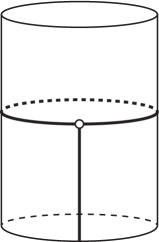
Figure 1: Graphical interpretation of the Lüscher correction is shown. Solid thick line represents the physical particle which arrives from the infinite past and is absorbed by the operator represented by a solid circle. The trajectory of a virtual (mirror) particle is represented by a half solid, half dashed ellipse. The operator emits this virtual particle, which travels around the world and is absorbed by the operator again leading to a 3-particle form factor.

There could be other ways to check our results, or its generalizations for the sine-Gordon theory. As the sine-Gordon theory is the continuum limit of the inhomogenous XXZ spin chain one could calculate the relevant vacuum-one-particle from factor on the lattice and evaluate carefully its continuum limit. The works Boos:2016yql ; Hegedus:2017zkz ; Hegedus:2017muz can be relevant in this direction.

The original purpose of the perturbative calculations was to check our main result (3.43), which gives the first Lüscher correction of the 1-particle form factor. Indeed, the second order form factor formula (4.13) is perfectly reproduced by (5.60) obtained by Hamiltonian perturbation theory. Equivalently we have checked (C.40), analytically for $q=0$ and numerically for $q\not=0$, in Lagrangian perturbation theory. The perturbative calculations actually go beyond the Lüscher approximation because they are exact in the volume. Indeed, the volume-exact second order energy formula (5.38) exactly matches (A.22), obtained from the TBA equations. Our perturbative form factor calculations can be used to check any future result (or conjecture) for a volume-exact 1-particle form factor. For this purpose one can use the formula (C.52), which can be evaluated numerically.

Clearly our novel result for the Lüscher correction of the simplest non-diagonal finite volume form factor is just a first step in calculating exactly the finite size corrections of form factors. We have projects to extend our result for generic non-diagonal form factors and also for their second Lüscher correction. However, in a long term, one should relate the appearing quantities to infinite volume form factors and the TBA densities similarly how it is done for the one-point function Leclair:1999ys and for the diagonal finite volume form factors Pozsgay:2013jua ; Pozsgay:2014gza .

Our results are relevant not only for two-dimensional integrable models, but via the AdS/CFT correspondence they can provide exact information for the string vertex in the $AdS_{5}\times S^{5}$ background Bajnok:2015hla and also on 3-point function in the maximally supersymmetric 4 dimensional gauge theory Komatsu:2017buu . The string vertex describes a process in which a big string splits into two smaller ones. The integrable description decompactifies the strings by cutting the pair of pants worldsheet into several parts Bajnok:2017mdf . Introducing one cut we obtain the decompactified string vertex, two cuts leads to the octagon amplitude, while introducing three cuts splits the worldsheet into two hexagons Basso:2015eqa . To reach an exact description the cut pieces have to be glued back again Basso:2015zoa ; Eden:2015ija . These include the introduction of a pair of virtual (mirror) particle states. Unfortunately the amplitude, as it stands, is divergent and one has to figure out how to regulate it Basso:2017muf . This is exactly what we figured out in the case when the cylinder with a local operator insertion was cut into a square as we started to glue it back by introducing a single pair of virtual particles.

Acknowledgments

This investigation was supported by the Hungarian National Science Fund NKFIH (under K116505) and by a Lendület Grant.

Appendix A Perturbative expansion of the sinh-Gordon TBA equations

In this appendix we expand analytically the sinh-Gordon vacuum and excited state TBA equations in the coupling. As the zeroth order term of the TBA kernel is the Dirac delta function one has to be careful. One can either explicitly subtract this term and then make the expansion, or alternatively it is also possible to shift the integration contour, to take additionally into account the pole of the kernel and expand the shifted equations with the new source term. We performed both calculations and got the same result, which we present now.

The vacuum TBA is an integral equation for the unknown function $Y^{(0)}(u)$ and is of the form

$$Y^{(0)}(u)={\rm e}^{-mL\cosh u}\exp\left\{\frac{1}{2\pi}\int_{-\infty}^{\infty}{\rm d}v\,\sigma(u-v)L^{(0)}(v)\right\},$$ (A.1)

where

$$L^{(0)}=\ln[1+Y^{(0)}]$$ (A.2)

and

$$\sigma(u)=\frac{2\alpha\cosh u}{\sinh^{2}u+\alpha^{2}}.$$ (A.3)

This TBA corresponds to the S-matrix

$$S(\theta)=\frac{\sinh\theta-i\alpha}{\sinh\theta+i\alpha}.$$ (A.4)

We will use the parameter $\alpha$ as our expansion parameter. The solution of (A.1) can be used to calculate the ground state energy, which is given by

$$E^{(0)}=-\frac{m}{2\pi}\int_{-\infty}^{\infty}{\rm d}u\,\cosh uL^{(0)}(u).$$ (A.5)

Similarly, the unknown function in the 1-particle TBA is $Y^{(1)}(u,\gamma)$, which satisfies

$$Y^{(1)}(u,\gamma)=\Sigma(u-\gamma){\rm e}^{-mL\cosh u}\exp\left\{\frac{1}{2\pi}\int_{-\infty}^{\infty}{\rm d}v\,\sigma(u-v)L^{(1)}(v,\gamma)\right\},$$ (A.6)

where

$$L^{(1)}=\ln[1+Y^{(1)}]$$ (A.7)

and

$$\Sigma(u)=\frac{\cosh u-\alpha}{\cosh u+\alpha}.$$ (A.8)

Let us introduce

$$D(\gamma)=mL\sinh\gamma-\frac{1}{2\pi}\int_{-\infty}^{\infty}{\rm d}u\,\tilde{\sigma}(u-\gamma)L^{(1)}(u,\gamma),$$ (A.9)

where

$$\tilde{\sigma}(u)=\frac{2\alpha\sinh u}{\cosh^{2}u-\alpha^{2}}.$$ (A.10)

The exact rapidity $\beta$ is defined to be the solution of the exact Bethe-Yang equation

$$D(\beta)=\frac{2\pi}{L}n=mL\sinh\theta.$$ (A.11)

We have to solve the coupled system (A.6) and (A.11) to calculate the energy of the first excited state with momentum

$$q=m\sinh\theta.$$ (A.12)

It is given by

$$E^{(1)}=m\cosh\beta-\frac{m}{2\pi}\int_{-\infty}^{\infty}{\rm d}u\,\cosh uL^{(1)}(u,\beta).$$ (A.13)

Finally the 1-particle spectrum is given by

$$E(q)=E^{(1)}(q)-E^{(0)}=E_{0}(q)+\alpha E_{1}(q)+\alpha^{2}E_{2}(q)+\dots$$ (A.14)

and the density of states by

$$R(q)=D^{\prime}(\beta)=R_{0}(q)+\alpha R_{1}(q)+\alpha^{2}R_{2}(q)+\dots$$ (A.15)

We can now perturbatively solve the TBA equations and after a long computation we find that the expansion coefficients can be expressed in terms of the following integrals:

$$f_{k}(q)=\frac{1}{\pi}\int_{-\infty}^{\infty}{\rm d}u\,\frac{1}{{\rm e}^{mL\cosh u}-1}\,\frac{1}{\cosh^{k}w},$$ (A.16)

$$g_{k}(q)=\frac{1}{\pi}\int_{-\infty}^{\infty}{\rm d}u\,\frac{1}{{\rm e}^{mL\cosh u}-1}\,\frac{\sinh w}{\cosh^{k}w},$$ (A.17)

$$\xi_{1}(q)=\frac{1}{\pi}\int_{-\infty}^{\infty}{\rm d}u\,\frac{{\rm e}^{mL\cosh u}}{({\rm e}^{mL\cosh u}-1)^{2}}\,\frac{1}{\cosh w},$$ (A.18)

where

$$w=u-\theta.$$ (A.19)

We will also use

$$\rho=2f_{0},$$ (A.20)

which has been introduced earlier in the bulk of the paper.

The expansion coefficients are

$$E_{0}(q)=m\cosh\theta,\qquad\qquad E_{1}(q)=\frac{m\rho}{2\cosh\theta},$$ (A.21)

$$E_{2}(q)=m\left\{-\left(\frac{1}{\cosh\theta}+\frac{mL\rho}{2}\right)\xi_{1}+(1+\tanh^{2}\theta)\frac{\rho^{2}}{8\cosh\theta}-\frac{\rho f_{2}}{2\cosh\theta}\right\}$$ (A.22)

and

$$R_{0}(q)=mL\cosh\theta,\qquad\qquad R_{1}(q)=mL\left\{\frac{\rho}{2\cosh\theta}-\cosh\theta f_{2}\right\},$$ (A.23)

$$R_{2}(q)=4f_{2}-6f_{4}-2\tanh\theta g_{3}+mL\left\{\left(\frac{1}{\cosh\theta}-\frac{1}{2\cosh^{3}\theta}\right)\frac{\rho^{2}}{4}+\cosh\theta f_{2}^{2}-\frac{\rho f_{2}}{\cosh\theta}\right\}.$$ (A.24)

In the Lüscher approximation these coefficients agree with those we get from the $\alpha$-expansion of the formulas (2.10) and (2.1):

$$\overline{E}_{1}(q)=\frac{m\bar{\rho}}{2\cosh\theta}=\frac{m}{\pi\cosh\theta}\int_{-\infty}^{\infty}{\rm d}u\,{\rm e}^{-mL\cosh u},$$ (A.25)

$$\overline{E}_{2}(q)=-\frac{m\bar{\xi}_{1}}{\cosh\theta}=-\frac{m}{\pi\cosh\theta}\int_{-\infty}^{\infty}{\rm d}u\,{\rm e}^{-mL\cosh u}\frac{1}{\cosh w},$$ (A.26)

$$\begin{split}\overline{R}_{1}(q)&=mL\left\{\frac{\bar{\rho}}{2\cosh\theta}-\cosh\theta\bar{f}_{2}\right\}\\ &=-\frac{mL}{\pi}\int_{-\infty}^{\infty}{\rm d}u\,{\rm e}^{-mL\cosh u}\sinh u\left[\tanh\theta\frac{1}{\cosh w}-\frac{\sinh w}{\cosh^{2}w}\right],\end{split}$$ (A.27)

$$\begin{split}\overline{R}_{2}(q)&=4\bar{f}_{2}-6\bar{f}_{4}-2\tanh\theta\bar{g}_{3}\\ &=\frac{mL}{\pi}\int_{-\infty}^{\infty}{\rm d}u\,{\rm e}^{-mL\cosh u}\sinh u\left[\tanh\theta\frac{1}{\cosh^{2}w}-\frac{2\sinh w}{\cosh^{3}w}\right].\end{split}$$ (A.28)

We always use an overline notation to indicate the Lüscher approximation of the same quantity.

Appendix B Details of the Hamiltonian perturbative calculations

In this appendix we explain how we turned the double sums in the Hamiltonian perturbation theory to integrals and how we performed their large volume expansions.

B.1 The double sum in the energy correction

In this part we provide an integral representation for the double sum

$$\sum_{k_{1}\in\mathbb{Z}}\sum_{k_{2}\neq n_{q}}D_{1}\left(k_{1},k_{2}\right)$$ (B.1)

with

$$D_{1}(k_{1},k_{2})= \;\frac{1}{\omega_{k_{1}}\omega_{k_{2}}\omega_{k_{1}+k_{2}-n_{q}}}\left(\frac{1}{\omega_{k_{1}}+\omega_{k_{2}}+\omega_{k_{1}+k_{2}-n_{q}}+\omega_{n_{q}}}\right.$$ (B.2)

$$\left.+\frac{1}{\omega_{k_{1}}+\omega_{k_{2}}+\omega_{k_{1}+k_{2}-n_{q}}-\omega_{n_{q}}}\right)$$ (B.3)

We start by applying the residue method to the $k_{1}$ variable. The analytically continued function $D_{1}\left(z,k_{2}\right)$ contains two pairs of branch cuts on the $z$ plane, starting from $\pm i\mu$ and $q-\frac{2\pi k_{2}}{L}\pm i\mu$, and going away from the real axis towards complex infinity in the imaginary direction. The integrals coming from the cuts below the real axis can be combined nicely to those above the real axis after a change of integration variable. Introducing $\kappa_{2}=2\pi k_{2}L^{-1}$, the resulting integral can be written as

$$\sum_{k_{1}\in\mathbb{Z}}\sum_{k_{2}\neq n_{q}}D_{1}\left(k_{1},k_{2}\right) = \sum_{k_{2}\neq n_{q}}\intop_{1}^{\infty}du\>i\mu\frac{L}{2\pi}\coth\left(\frac{\mu Lu}{2}\right)\left(\Theta_{q,\mu}\left(\kappa_{2}-q,u\right)+\Delta_{q,\mu}\left(\kappa_{2},u\right)\right.$$ (B.4)

$$\left.+\Theta_{q,\mu}\left(\kappa_{2}-q,-u\right)+\Delta_{q,\mu}\left(\kappa_{2},-u\right)\right)$$

where

$$\Theta_{q,\mu}\left(\kappa,u\right)=\frac{\kappa\left(\mu+iqu\right)-\mu q\left(u^{2}-1\right)}{\kappa\mu^{2}\left(\kappa+q+i\mu u\right)\left(iq+\mu u\right)\sqrt{\left(u^{2}-1\right)\left(\mu^{2}+\left(\kappa+i\mu u\right)^{2}\right)}}$$ (B.5)

and

$$\Delta_{q,\mu}\left(\kappa,u\right)=-\frac{\kappa qu+\mu^{2}u+i\mu q-i\kappa\mu}{\mu^{2}\left(\kappa-q\right)\left(q-i\mu u\right)\left(\kappa+i\mu u\right)\sqrt{\left(u^{2}-1\right)\left(\mu^{2}+\kappa^{2}\right)}}$$ (B.6)

We now turn the remaining summation to integration.

We note that in (B.4) both $\Theta_{q,\mu}$ and $\Delta_{q,\mu}$ having $+u$ argument are the contributions of the branch cuts starting from $+i\mu$ and $-i\mu+q-\kappa_{2}$, whereas the terms of $-u$ argument correspond to the other two cuts. Interchanging the $k_{2}$ sum with the integral, the remaining sums to be evaluated have the form

$$S_{\Theta} = \sum_{k_{2}\neq n_{q}}\left[\Theta_{q,\mu}\left(\kappa_{2}-q,u\right)+\Theta_{q,\mu}\left(\kappa_{2}-q,-u\right)\right]$$ (B.7)

$$= \sum_{k_{2}\neq 0}\left[\Theta_{q,\mu}\left(\kappa_{2},u\right)+\Theta_{q,\mu}\left(\kappa_{2},-u\right)\right]$$ (B.8)

$$= \sum_{k_{2}\neq 0}\left[\Theta_{q,\mu}\left(\kappa_{2},u\right)+\Theta_{q,\mu}\left(-\kappa_{2},-u\right)\right]$$ (B.9)

$$= \sum_{k_{2}\neq 0}\frac{2u\left(\mu^{2}+q^{2}\right)\left(\kappa_{2}+i\mu u\right)}{\mu^{2}(q^{2}+\mu^{2}u^{2})\left[(\kappa_{2}+i\mu u)^{2}-q^{2}\right]\sqrt{\left(u^{2}-1\right)\left[\mu^{2}+\left(\kappa_{2}+i\mu u\right)^{2}\right]}}$$ (B.10)

and

$$S_{\Delta} = \sum_{k_{2}\neq n_{q}}\left[\Delta_{q,\mu}\left(\kappa_{2},u\right)+\Delta_{q,\mu}\left(\kappa_{2},-u\right)\right]$$ (B.11)

$$= -\sum_{k_{2}\neq n_{q}}\frac{2i\kappa_{2}q\sqrt{u^{2}-1}}{\mu\omega_{k_{2}}\left(\kappa_{2}^{2}+\mu^{2}u^{2}\right)\left(q^{2}+\mu^{2}u^{2}\right)}$$ (B.12)

$$= \frac{2iq^{2}\sqrt{u^{2}-1}}{\mu\omega_{n_{q}}\left(q^{2}+\mu^{2}u^{2}\right)^{2}}$$ (B.13)

where in the last step we used the antisymmetry of the summand.

We now proceed by obtaining an integral representation of the sum $S_{\Theta}$. Analytically continuing the summand of (B.10) into the complex $\kappa_{2}$ plane, we find a pair of branch cuts and two single poles. However, this time the branch points of the cuts lie at $i\mu\left(\pm 1-u\right)$, and since $u>1$, the upper cut intersects the real axis. The $k_{2}=n_{q}$ terms of the double sum in (5.30) were separated for precisely this reason. Now an integral representation can be achieved by writing $S_{\Theta}$ as a sum of two contour integrals

$$S_{\Theta}=\frac{L}{2\pi}\left[\intop_{C_{1}}dz\frac{e^{iLz}}{e^{iLz}-1}f_{\Theta}\left(z\right)+\intop_{C_{2}}dz\frac{e^{iLz}}{e^{iLz}-1}f_{\Theta}\left(z\right)\right]$$ (B.14)

with

$$f_{\Theta}\left(z\right)=\frac{2u\left(\mu^{2}+q^{2}\right)\left(z+i\mu u\right)}{\mu^{2}\left(z-q+i\mu u\right)\left(z+q+i\mu u\right)\left(q^{2}+\mu^{2}u^{2}\right)\sqrt{\left(u^{2}-1\right)\left[\mu^{2}+\left(z+i\mu u\right)^{2}\right]}}.$$ (B.15)

The closed contours $C_{1}$ and $C_{2}$ are chosen such that $C_{1}$ goes from $-\infty-i\epsilon$ to $-2\pi L^{-1}-i\epsilon$ just below the real axis, then from $-2\pi L^{-1}+i\epsilon$ back to $-\infty+i\epsilon$ just above the real axis, while $C_{2}$ is the mirror image of $C_{1}$ with respect to the imaginary axis except that it is also directed counterclockwise. Now both contours can be blown up such that they are tightened to the cuts. As a result of the deformation, the poles of $f_{\Theta}$ at $z=\pm q-i\mu u$ become encircled in the negative direction which results in additional residual terms. After the variable changes $u\rightarrow\cosh u$, $v\rightarrow\cosh v$, and extending the intagration domain over the real line by symmetrization, we get an integral representation of $S_{\Theta}$ as

$$S_{\Theta} = \frac{2L}{i\mu^{2}}\frac{e^{\mu Lu}}{e^{\mu Lu}-1}\frac{\sqrt{\mu^{2}+q^{2}}u}{\left(q^{2}+\mu^{2}u^{2}\right)\sqrt{u^{2}-1}}+\frac{L}{i\pi\mu}\intop_{-\infty}^{\infty}dv\left(\lambda\left(u,v\right)s\left(u,v\right)+\mathrm{sing}_{\Theta}\left(u,v\right)\right)\quad\quad$$ (B.16)

where

$$\lambda\left(u,v\right) = \frac{e^{\mu L\cosh u}}{e^{\mu L\cosh v}-e^{\mu L\cosh u}}-\frac{e^{\mu L\left(\cosh u+\cosh v\right)}}{e^{\mu L\left(\cosh u+\cosh v\right)}-1},$$ (B.17)

$$s\left(u,v\right) = \frac{\left(\mu^{2}+q^{2}\right)\cosh u\cosh v}{\left(q^{2}+\mu^{2}\cosh^{2}u\right)\left(q^{2}+\mu^{2}\cosh^{2}v\right)},$$ (B.18)

$$\mathrm{sing}_{\Theta}\left(u,v\right) = \frac{2}{\mu L}\frac{1}{u^{2}-v^{2}}\frac{s\left(u,u\right)u}{\sinh u}$$ (B.19)

The term of (B.19) comes from the neighbourhood of the branch-overlapped pole. Note that both $\lambda\left(u,v\right)$ and $\mathrm{sing}_{\Theta}\left(u,v\right)$ are singular along the lines $u=\pm v$; their sum is, however, finite everywhere.

At this stage, we can represent the original double sum as a formula containing the following double integral

$$\sum_{k_{1},k_{2}\in\mathbb{Z}}D_{1}\left(k_{1},k_{2}\right) = L^{2}\intop_{-\infty}^{\infty}\frac{du}{2\pi}\intop_{-\infty}^{\infty}\frac{dv}{2\pi}\coth\left(\frac{\mu L}{2}\cosh u\right)\left(\lambda\left(u,v\right)s\left(u,v\right)+\mathrm{sing}_{\Theta}\left(u,v\right)\right)$$ (B.20)

$$+\left(\text{other terms}\right)$$

Since the double integral is absolutely convergent, we can perform a symmetrization of the integrand as

$$\intop_{-\infty}^{\infty}\intop_{-\infty}^{\infty}dudv\>f\left(u,v\right)=\frac{1}{2}\intop_{-\infty}^{\infty}\intop_{-\infty}^{\infty}dudv\>\left(f\left(u,v\right)+f\left(v,u\right)\right)$$ (B.21)

which leaves the value of the integral unchanged. Upon this transformation, the first term of (B.20) becomes

$$L^{2}\intop_{-\infty}^{\infty}\frac{du}{2\pi}\intop_{-\infty}^{\infty}\frac{dv}{2\pi}\frac{1+e^{\mu L\cosh u}+e^{\mu L\cosh v}-3e^{\mu L\left(\cosh u+\cosh v\right)}}{2\left(e^{\mu L\cosh u}-1\right)\left(e^{\mu L\cosh v}-1\right)}s\left(u,v\right)$$ (B.22)

which can be further simplified as

$$L^{2}\intop_{-\infty}^{\infty}\frac{du}{2\pi}\intop_{-\infty}^{\infty}\frac{dv}{2\pi}\frac{1+e^{\mu L\cosh u}+e^{\mu L\cosh v}-3e^{\mu L\left(\cosh u+\cosh v\right)}}{2\left(e^{\mu L\cosh u}-1\right)\left(e^{\mu L\cosh v}-1\right)}s\left(u,v\right) =$$

$$-\frac{L^{2}}{\mu^{2}}\left(\frac{3}{8}+\intop_{-\infty}^{\infty}\frac{du}{2\pi}\frac{1}{e^{\mu L\cosh u}-1}\frac{\mu\sqrt{\mu^{2}+q^{2}}\cosh u}{q^{2}+\mu^{2}\cosh^{2}u}\right)$$ (B.23)

if we note that

$$\frac{1+e^{\mu L\cosh u}+e^{\mu L\cosh v}-3e^{\mu L\left(\cosh u+\cosh v\right)}}{2\left(e^{\mu L\cosh u}-1\right)\left(e^{\mu L\cosh v}-1\right)}=-\frac{3}{2}-\frac{1}{e^{\mu L\cosh u}-1}-\frac{1}{e^{\mu L\cosh v}-1}$$ (B.24)

We now calculate the integral of the symmetrized second term of the integrand. For brevity, we introduce the function

$$\mathrm{sing}\left(u,v\right)=\coth\left(\frac{\mu L}{2}\cosh u\right)\mathrm{sing}_{\Theta}\left(u,v\right).$$

In this notation, the symmetrized integral has the following form

$$\frac{L^{2}}{2}\intop_{-\infty}^{\infty}\frac{du}{2\pi}\intop_{-\infty}^{\infty}\frac{dv}{2\pi}\left(\mathrm{sing}\left(u,v\right)+\mathrm{sing}\left(v,u\right)\right).$$

Both terms of this integrand are divergent by themselves; their sum, however, is finite everywhere. To perform the integrations, we notice that due to the symmetry of the integrand,

$$\frac{L^{2}}{2}\intop_{-\infty}^{\infty}\frac{du}{2\pi}\intop_{-\infty}^{\infty}\frac{dv}{2\pi}\left(\mathrm{sing}\left(u,v\right)+\mathrm{sing}\left(v,u\right)\right)=\frac{4L^{2}}{2}\intop_{0}^{\infty}\frac{du}{2\pi}\intop_{-u}^{u}\frac{dv}{2\pi}\left(\mathrm{sing}\left(u,v\right)+\mathrm{sing}\left(v,u\right)\right)$$ (B.25)

which we regularize as

$$2L^{2}\lim_{\epsilon\rightarrow 0}\left[\intop_{\epsilon}^{\infty}\frac{du}{2\pi}\intop_{-u+\epsilon}^{u-\epsilon}\frac{dv}{2\pi}\mathrm{sing}\left(u,v\right)+\intop_{\epsilon}^{\infty}\frac{du}{2\pi}\intop_{-u+\epsilon}^{u-\epsilon}\frac{dv}{2\pi}\mathrm{sing}\left(v,u\right)\right] =$$

$$2L^{2}\lim_{\epsilon\rightarrow 0}\left[\intop_{\epsilon}^{\infty}\frac{du}{2\pi}\intop_{-u+\epsilon}^{u-\epsilon}\frac{dv}{2\pi}\mathrm{sing}\left(u,v\right)+2\intop_{0}^{\infty}\frac{du}{2\pi}\intop_{u+\epsilon}^{\infty}\frac{dv}{2\pi}\mathrm{sing}\left(u,v\right)\right]$$ (B.26)

In the last step we made use of the identity

$$\intop_{\epsilon}^{\infty}\frac{du}{2\pi}\intop_{-u+\epsilon}^{u-\epsilon}\frac{dv}{2\pi}=\intop_{-\infty}^{\infty}\frac{dv}{2\pi}\intop_{v+\epsilon}^{\infty}\frac{du}{2\pi},$$ (B.27)

and the fact that $\mathrm{sign}\left(u,v\right)$ is symmetric in $v$ together with the freedom to switch the labeling of integration variables. Now the integrals over $v$ in (B.26) can be performed. Combining the remaining $u$ integrals, we obtain

$$\frac{8L}{\mu}\lim_{\epsilon\rightarrow 0}\left[-\intop_{0}^{\epsilon}\frac{du}{\left(2\pi\right)^{2}}\frac{\tilde{s}\left(u\right)}{\sinh u}\mathrm{arctanh}\left(\frac{u}{u+\epsilon}\right)+\frac{1}{2}\intop_{\epsilon}^{\infty}\frac{du}{\left(2\pi\right)^{2}}\frac{\tilde{s}\left(u\right)}{\sinh u}\ln\left(1-\frac{2\epsilon}{\epsilon+2u}\right)\right]$$ (B.28)

with

$$\tilde{s}\left(u\right)=s\left(u,u\right)\coth\left(\frac{\mu L}{2}\cosh u\right).$$ (B.29)

Both integrands approximate Dirac $\delta$-like peaks centered at $u=0$ in the $\epsilon\rightarrow 0$ limit. Thus, we approximate the regular part $\tilde{s}\left(u\right)$ with its value at the top of the peaks, and integrate analytically the singular part. Finally, taking the $\epsilon\rightarrow 0$ limit, we get

$$\frac{L^{2}}{2}\intop_{-\infty}^{\infty}\frac{du}{2\pi}\intop_{-\infty}^{\infty}\frac{dv}{2\pi}\left(\mathrm{sing}\left(u,v\right)+\mathrm{sing}\left(v,u\right)\right)=\; \frac{L}{\mu\left(\mu^{2}+q^{2}\right)\pi^{2}}\coth\left(\frac{\mu L}{2}\right)\bigg{(}\mathrm{Li}_{2}\left(-2\right)$$ (B.30)

$$+\frac{1}{2}\mathrm{Li}_{2}\left(\frac{1}{4}\right)-\frac{\pi^{2}}{6}+\left(\ln\>2\right)^{2}\bigg{)}$$ (B.31)

where $\mathrm{Li}_{2}\left(x\right)$ is the dilogarithm function

$$\mathrm{Li}_{2}\left(x\right)=\intop_{0}^{\infty}\frac{t}{e^{t}/x-1},\quad x\in\mathbb{C}\setminus\left\{x\in\mathbb{R}\wedge x\geq 1\right\}.$$ (B.32)

Using the above integral representation, the Abel identity

$$\mathrm{Li}_{2}\left(\frac{x}{1-y}\right)+\mathrm{Li}_{2}\left(\frac{y}{1-x}\right)-\mathrm{Li}_{2}\left(\frac{xy}{\left(1-x\right)\left(1-y\right)}\right)=\mathrm{Li}_{2}\left(x\right)+\mathrm{Li}_{2}\left(y\right)+\ln\left(1-x\right)\ln\left(1-y\right)$$ (B.33)

with $x=-1$ and $y=\frac{1}{2}$, and the special value

$$\mathrm{Li}_{2}\left(-1\right)=-\frac{\pi^{2}}{12},$$ (B.34)

we obtain

$$\mathrm{Li}_{2}\left(-2\right)+\frac{1}{2}\mathrm{Li}_{2}\left(\frac{1}{4}\right)-\frac{\pi^{2}}{6}+\left(\ln\>2\right)^{2}=-\frac{\pi^{2}}{4}$$ (B.35)

Putting everything together, the double sum of (5.30) can be written as

$$\sum_{k_{1},k_{2}\in\mathbb{Z}}D_{1}\left(k_{1},k_{2}\right)=C_{1}+C_{2}+C_{\Delta}+C_{r}+C_{ord}+C_{sing}$$ (B.36)

where:

• $C_{1}$ and $C_{2}$ contains the single sums separated in (5.30). Using (5.29) and (5.31),

  $$C_{1} = \frac{L}{\omega_{n_{q}}\mu^{2}}\left(\frac{1}{2\pi}+\mu L\intop_{-\infty}^{\infty}\frac{du}{2\pi}\frac{e^{\mu L\cosh u}}{\left(e^{\mu L\cosh u}-1\right)^{2}}\cosh u\right)$$ (B.37)

  $$C_{2} = \frac{L}{4\omega_{n_{q}}^{2}\mu}\coth\left(\frac{\mu L}{2}\right)-\frac{L}{2\omega_{n_{q}}}\intop_{-\infty}^{\infty}\frac{du}{2\pi}\frac{\coth\left(\frac{\mu L}{2}\cosh u\right)}{\omega_{n_{q}}^{2}+\mu^{2}\sinh^{2}u}$$ (B.38)

• $C_{\Delta}$ stands for the term coming from (B.13)

  $$C_{\Delta}=-\intop_{-\infty}^{\infty}\frac{du}{2\pi}\>\frac{L}{\omega_{n_{q}}}\coth\left(\frac{\mu L\cosh u}{2}\right)\frac{q^{2}\sinh^{2}u}{\left(q^{2}+\mu^{2}\cosh^{2}u\right)^{2}}$$ (B.39)

• $C_{r}$ contains the residual terms emerging from the contour deformation of the integral representation of $S_{\Theta}$ appearing in (B.16)

  $$C_{r}=\intop_{-\infty}^{\infty}\frac{du}{2\pi}\>\frac{L^{2}}{\mu}\coth\left(\frac{\mu L\cosh u}{2}\right)\frac{e^{\mu L\cosh u}}{e^{\mu L\cosh u}-1}\frac{\sqrt{\mu^{2}+q^{2}}\cosh u}{\left(q^{2}+\mu^{2}\cosh^{2}u\right)}$$ (B.40)

• $C_{ord}$ is the symmetrized double integral contribution (B.23)

  $$C_{ord}=-\frac{L^{2}}{\mu^{2}}\left(\frac{3}{8}+\intop_{-\infty}^{\infty}\frac{du}{2\pi}\frac{1}{e^{\mu L\cosh u}-1}\frac{\mu\sqrt{\mu^{2}+q^{2}}\cosh u}{q^{2}+\mu^{2}\cosh^{2}u}\right)$$ (B.41)

• Finally, $C_{sing}$ is the symmetrized singular contribution (B.31)

  $$C_{sing}=-\frac{L}{4\mu\left(\mu^{2}+q^{2}\right)}\coth\left(\frac{\mu L}{2}\right).$$ (B.42)

Combining these terms, significant simplifiactions can be achieved. First of all, notice that $C_{sing}$ is cancelled by a similar term appearing in $C_{2}$. As a next step, we combine $C_{\Delta}$ and the integral part of $C_{2}$, and perform integration by parts. The resulting boundary term cancels the explicit term appearing in $C_{1}$. $C_{r}$ contains an infinite-volume term that can be separated and integrated analytically. Then, the remaining part of the integral in $C_{r}$, the integral part of $C_{ord}$, the integral appearing in $C_{1}$ and the result of the previous integration by parts can be combined beautifully together and lead to the following nice representation of the full double sum:

$$\sum_{k_{1},k_{2}}D_{1}\left(k_{1},k_{2}\right)=\frac{L^{2}}{\mu^{2}}\left(\frac{1}{8}+3\intop_{-\infty}^{\infty}\frac{du}{2\pi}\frac{e^{\mu L\cosh u}}{\left(e^{\mu L\cosh u}-1\right)^{2}}\frac{1}{\cosh\left(u-\theta\right)}\right)$$ (B.43)

where we introduced $\theta$ as the rapidity variable $q=\mu\sinh\theta$.

B.2 Expansion of the form factor

We first provide an integral representation of the double sum $\sum_{k_{1},k_{2}}D_{2}\left(k_{1},k_{2}\right)$ , we then calculate the large volume expansion of the full form factor $\left\langle 0\left(b\right)\left|\varphi\right|q\left(b\right)\right\rangle$.

The transformation of

$$\sum_{k_{1},k_{2}}D_{2}\left(k_{1},k_{2}\right)$$ (B.44)

with

$$D_{2}\left(k_{1},k_{2}\right)=\; \frac{1}{\omega_{k_{1}}\omega_{k_{2}}\omega_{k_{1}+k_{2}-n_{q}}}\bigg{[}\Bigl{(}\frac{1}{\omega_{k_{1}}+\omega_{k_{2}}+\omega_{k_{1}+k_{2}-n_{q}}+\omega_{n_{q}}}\Bigr{)}^{2}$$ (B.45)

$$-\Bigl{(}\frac{1}{\omega_{k_{1}}+\omega_{k_{2}}+\omega_{k_{1}+k_{2}-n_{q}}-\omega_{n_{q}}}\Bigr{)}^{2}\bigg{]}$$ (B.46)

can be started in parallel to the steps done in the case of $D_{1}\left(k_{1},k_{2}\right)$. We first separate the $k_{2}=n_{q}$ terms analogously to (5.30)

$$\sum_{k_{1},k_{2}\in\mathbb{Z}}D_{2}\left(k_{1},k_{2}\right)=\sum_{k_{1}\in\mathbb{Z}}\sum_{k_{2}\neq n_{q}}D_{2}\left(k_{1},k_{2}\right)-\frac{1}{4\omega_{n_{q}}}\sum_{k_{1}\in\mathbb{Z}}\frac{1}{\omega_{k_{1}}^{4}}+\frac{1}{4\omega_{n_{q}}}\sum_{k_{1}\in\mathbb{Z}}\frac{1}{\omega_{k_{1}}^{2}}\frac{1}{\left(\omega_{k_{1}}+\omega_{n_{q}}\right)^{2}}$$ (B.47)

These separated terms can be easily calculated using the derivative of (5.31) with respect to $A$ and the formula

$$\sum_{k\in\mathbb{Z}}\frac{1}{\omega_{k}^{4}}=\frac{2L\coth\left(\frac{\mu L}{2}\right)+\mu L^{2}\mathrm{csch}^{2}\left(\frac{\mu L}{2}\right)}{8\mu^{3}}.$$ (B.48)

Now we turn the sum over $k_{1}$ into an integral. This can be done in a straightforward manner. Using the variable $\kappa_{2}=2\pi k_{2}L^{-1}$, we get

$$\sum_{k_{1}\in\mathbb{Z}}\sum_{k_{2}\neq n_{q}}D_{2}\left(k_{1},k_{2}\right)= \sum_{k_{2}\neq n_{q}}\frac{L}{2\pi}\intop_{-\infty}^{\infty}du\coth\left(\frac{\mu L}{2}\cosh u\right)\left(\Xi\left(k_{2},\omega_{n_{q}},q\right)\right.$$ (B.49)

$$\left.+\Xi\left(k_{2},\omega_{n_{q}},-q\right)-\Xi\left(k_{2},-\omega_{n_{q}},q\right)-\Xi\left(k_{2},-\omega_{n_{q}},-q\right)\right)$$ (B.50)

with

$$\Xi\left(k_{2},A,q\right)=\frac{\left(\sqrt{\mu^{2}+\left(q-\kappa_{2}\right)^{2}}+\sqrt{\mu^{2}+\left(\kappa_{2}+i\mu\cosh u\right)^{2}}-i\mu\sinh u+A\right)^{-2}}{\sqrt{\mu^{2}+\left(q-\kappa_{2}\right)^{2}}\sqrt{\mu^{2}+\left(\kappa_{2}+i\mu\cosh u\right)^{2}}}.$$ (B.51)

By means of equivalent transformations including a shift of the summation variable $\kappa_{2}=\tilde{\kappa}_{2}+q$, symmetrization of the integrand and algebraic manipulations, (B.50) simplifies miraculously to a sum of two terms, plus the same sum with the sign of $q$ switched, each term containing only a single pair of branch cuts:

$$\sum_{\begin{subarray}{c}k_{1}\in\mathbb{Z}\\ k_{2}\neq n_{q}\end{subarray}}D_{2}(k_{1},k_{2})= -\frac{L\omega_{n_{q}}}{16\mu^{2}}\sum_{k_{2}\neq 0}\intop_{-\infty}^{\infty}\frac{du}{2\pi}\bigg{[}\frac{\coth\big{(}\frac{\mu L}{2}\cosh u\big{)}}{\kappa_{2}^{2}(\kappa_{2}-q+i\mu\cosh u)^{2}(q+i\mu\cosh u)^{2}}$$ (B.52)

$$\times\Big{(}\mathcal{G}(\kappa_{2}-q,q)+\mathcal{G}(-\kappa_{2}-i\mu\cosh u,q)\Big{)}+(q\rightarrow-q)\bigg{]}$$ (B.53)

where

$$\mathcal{G}\left(x,q\right) = \frac{4\mu^{2}\left(x+q\right)^{2}-2i\mu P_{1}\left(x,q\right)\cosh u-2P_{2}\left(x,q\right)\left[2\left(x+q\right)\cosh 2u+i\mu\cosh 3u\right]}{\sqrt{\mu^{2}+x^{2}}}\quad\quad$$ (B.54)

$$P_{1}\left(x,q\right) = 4x^{3}+6x^{2}q+x\left(\mu^{2}+4q^{2}\right)-\mu^{2}q$$ (B.55)

$$P_{2}\left(x,q\right) = 2x^{2}q-x\mu^{2}+\mu^{2}q$$

Now we proceed to transform the remaining sum (over $k_{2}$) in these terms.

Let us first examine the sum containing $\mathcal{G}\left(\kappa_{2}-q\right)$. The arising complex function contains the usual set of poles on the real line and a pair of branch cuts starting from $z=\pm i\mu+q$ to complex infinity. It also has one pole of order 3 at $z=0$ and another of order 2 at $z=q-i\mu\cosh u$. The latter is overlapped by the lower branch cut. After the deformation of the contour, the pole of order 3 is encircled in the clockwise direction. Other finite terms come from the overlapped second-order pole which cancel the divergences of the branch cut integral. We obtain

$$-\frac{L\omega_{n_{q}}}{16\mu^{2}}\sum_{k_{2}\neq 0}\intop_{-\infty}^{\infty}\frac{du}{2\pi}\frac{\coth\left(\frac{\mu L}{2}\cosh u\right)\mathcal{G}\left(\kappa_{2}-q,q\right)}{\kappa_{2}^{2}\left(\kappa_{2}-q+i\mu\cosh u\right)^{2}\left(q+i\mu\cosh u\right)^{2}}=I_{1}^{+}\left(q\right)+I_{1}^{-}\left(q\right)+R_{1}\left(q\right)$$ (B.56)

where

$$I_{1}^{-}\left(q\right)=\; -\frac{L^{2}\omega_{n_{q}}}{8\mu^{2}}\intop_{-\infty}^{\infty}\frac{du}{2\pi}\intop\frac{dv}{2\pi}\bigg{[}\coth\Bigl{(}\frac{\mu L}{2}\cosh u\Bigr{)}\frac{e^{\mu L\cosh v}}{e^{\mu L\cosh v}-1}\frac{G\left(\cosh u,\cosh v,q\right)}{\left(\cosh u-\cosh v\right)^{2}}$$ (B.57)

$$+\mathrm{sing}_{1}\left(u,v,q\right)\bigg{]}$$ (B.58)

$$I_{1}^{+}\left(q\right)=\; -\frac{L^{2}\omega_{n_{q}}}{8\mu^{2}}\intop_{-\infty}^{\infty}\frac{du}{2\pi}\intop\frac{dv}{2\pi}\frac{\coth\left(\frac{\mu L}{2}\cosh u\right)}{e^{\mu L\cosh v}-1}\frac{G\left(\cosh u,-\cosh v,q\right)}{\left(\cosh u+\cosh v\right)^{2}}$$ (B.59)

$$R_{1}\left(q\right)=\; \frac{L}{192\mu^{2}}\intop_{-\infty}^{\infty}\frac{du}{2\pi}\frac{\coth\left(\frac{\mu L}{2}\cosh u\right)P_{R1}\left(\cosh u,q\right)}{\left(q-i\mu\cosh u\right)^{4}\left(q+i\mu\cosh u\right)^{2}}$$ (B.60)

with

$$G\left(x,y,q\right) = \frac{-4}{\left(q+i\mu x\right)^{2}\left(q-i\mu y\right)^{2}}\left[\mu^{2}xy\left(-1+x^{2}-xy+y^{2}\right)+q^{2}\left(1-xy-y^{2}+x^{2}\left(-1+2y^{2}\right)\right)\right.$$ (B.61)

$$\left.+i\mu q\left(x-y+y^{3}-2x^{2}y^{3}+x^{3}\left(-1+2y^{2}\right)\right)\right]$$

$$\mathrm{sing}_{1}\left(u,v,q\right)= -2\coth\left(\frac{\mu L}{2}\cosh u\right)\frac{e^{\mu L\cosh u}}{e^{\mu L\cosh u}-1}\left\{\frac{u^{2}+v^{2}}{\left(u^{2}-v^{2}\right)^{2}}\frac{G\left(\cosh u,\cosh u,q\right)}{\sinh^{2}u}\right.$$ (B.62)

$$+\frac{u}{\sinh u}\frac{1}{u^{2}-v^{2}}\left[\left(\frac{\mu L}{e^{\mu L\cosh u}-1}+\frac{\cosh u}{\sinh^{2}u}\right)G(\cosh u,\cosh u,q)\right.$$ (B.63)

$$\left.\left.-\frac{\partial G\left(\cosh u,y,q\right)}{\partial y}\bigg{|}_{y=\cosh u}\right]\right\}$$ (B.64)

and $P_{R1}\left(x,q\right)$ is some complicated polynomial of $x$,$q$,$L$ and $\mu$.

We can immediately calculate the infinite volume limit and first Lüscher correction of (B.56) and its opposite momentum pair. For the infinite volume limit, we can analytically take both integrals in (B.58) and (B.59). For the first Lüscher correction, one integral can be done analytically, and we are led to a formula containing only a single integral, as expected. We note that higher Lüscher corrections seem to be much harder to get in the form of explicit single-integral formulas. In the following, we use the rapidity variable $q=\mu\cosh\theta$.

The term $I_{1}^{+}\left(q\right)+I_{1}^{+}\left(-q\right)$ does not contribute to the infinite volume limit, and gives a first order Lüscher contribution

$$\widetilde{I_{1}^{+}} = \frac{L^{2}}{\pi\mu^{3}}\intop_{-\infty}^{\infty}\frac{du}{2\pi}\frac{e^{-\mu L\cosh u}}{\left(\cosh 2\theta+\cosh 2u\right)^{3}}\bigg{[}-\cosh\theta\Big{(}(3+\cosh 4\theta)\cosh 2u+\cosh 2\theta(3+\cosh 4u)\Big{)}$$ (B.65)

$$+\pi\cosh u(-3+\cosh 4\theta-2\cosh 2\theta\cosh 2u)\sinh^{2}u$$

$$-u\cosh\theta(-3+\cosh 4\theta-2\cosh 2\theta\cosh 2u)\sinh 2u$$

$$-\theta\cosh\theta(-3+\cosh 4u-2\cosh 2\theta\cosh 2u)\sinh 2\theta\bigg{]}$$

The term $I_{1}^{-}\left(q\right)+I_{1}^{-}\left(-q\right)$ has the infinite volume limit

$$I_{1}^{\infty}=\frac{L^{2}\left(\pi^{2}-4\right)\cosh\theta}{8\pi^{2}\mu^{3}}$$ (B.66)

and admits a first Lüscher correction

$$\widetilde{I_{1}^{-}} = \frac{3L^{2}}{\pi\mu^{3}}\intop_{-\infty}^{\infty}\frac{du}{2\pi}\frac{e^{-\mu L\cosh u}}{\left(\cosh 2\theta+\cosh 2u\right)^{3}}\bigg{[}-\cosh\theta\Big{(}\left(3+\cosh 4\theta\right)\cosh 2u+\cosh 2\theta\left(3+\cosh 4u\right)\Big{)}$$ (B.67)

$$-\pi\cosh u\left(-3+\cosh 4\theta-2\cosh 2\theta\cosh 2u\right)\sinh^{2}u$$

$$-u\cosh\theta\left(-3+\cosh 4\theta-2\cosh 2\theta\cosh 2u\right)\sinh 2u$$

$$-\theta\cosh\theta\left(-3+\cosh 4u-2\cosh 2\theta\cosh 2u\right)\sinh 2\theta\bigg{]}$$

The residual part $R_{1}\left(q\right)+R_{1}\left(-q\right)$ contributes to the infinite volume limit with

$$R_{1}^{\infty}=-\frac{L^{2}\cosh\theta}{8\mu^{3}}+\frac{L\left(-1+2\theta\coth 2\theta\right)}{\mu^{4}\pi\sinh^{2}2\theta}$$ (B.68)

while its first Lüscher correction is

$$\widetilde{R_{1}}=\; -\frac{L}{\mu^{4}}\intop_{-\infty}^{\infty}\frac{du}{2\pi}\frac{e^{-\mu L\cosh u}}{\left(\cosh 2u+\cosh 2\theta\right)^{4}}\bigg{[}-16+2\cosh 4\theta+\cosh 6u\cosh 2\theta$$ (B.69)

$$+\cosh 4u(2-4\cosh 4\theta)+\cosh 2u\left(-18\cosh 2\theta+\cosh 6\theta\right)\bigg{]}$$ (B.70)

$$-\frac{L^{2}}{\mu^{3}}\intop_{-\infty}^{\infty}\frac{du}{2\pi}\frac{e^{-\mu L\cosh u}}{(\cosh 2u+\cosh 2\theta)^{4}}2\cosh u\sinh^{2}u$$ (B.71)

$$\times\bigg{[}4\cosh 2u+\cosh 2\theta(4+\cosh 4u-\cosh 4\theta)\bigg{]}$$ (B.72)

To deal with the other sums of (B.52) containing $\mathcal{G}\left(-\kappa_{2}-i\mu\cosh u,q\right)$, it is expedient to desingularize the summand with a small auxiliary parameter $a$, in the following way:

$$-\frac{L\omega_{n_{q}}}{16\mu^{2}}\sum_{k_{2}\neq 0}\intop_{-\infty}^{\infty}\frac{du}{2\pi}\frac{\coth\left(\frac{\mu L}{2}\cosh u\right)\mathcal{G}\left(-\kappa_{2}-i\mu\cosh u,q\right)}{\left(\kappa_{2}-\mu a\right)\left(\kappa_{2}+\mu a\right)\left(\kappa_{2}-q+i\mu\cosh u\right)^{2}\left(q+i\mu\cosh u\right)^{2}}$$ (B.73)

$$= I_{2a}^{+}\left(q\right)+I_{2a}^{-}\left(q\right)+R_{2a}\left(q\right)$$ (B.74)

Here $I_{2a}^{+}\left(q\right)$ contains the upper branch cut integral surrounding a single pole, similar to the one arising in the computation of $D_{1}\left(k_{1},k_{2}\right)$, plus the sum of residues $r_{2a}\left(u,v,q\right)$ of regularized poles at $z=\pm\mu a$. $I_{2a}^{-}\left(q\right)$ denotes the lower, regular branch cut integral, while $R_{2a}\left(q\right)$ is the residual term coming from the pole at $z=q-i\mu\cosh u$. The limit $a\rightarrow 0$ can immediately be taken for $I_{2a}^{-}\left(q\right)$ and $R_{2a}\left(q\right)$, and the corresponding Lüscher- and infinite volume corrections are easily obtained (after the final momentum-combination) as

$$I_{2}^{-,\infty}=-\frac{L^{2}\left(4+\pi^{2}\right)\cosh\theta}{8\mu^{3}\pi^{2}}$$ (B.75)

$$\widetilde{I_{2}^{-}} = 2\widetilde{I_{1}^{+}}$$ (B.76)

$$R_{2}^{\infty}=\frac{L^{2}\cosh\theta}{4\mu^{3}}$$ (B.77)

$$\widetilde{R_{2}}= \,\frac{6L^{2}}{\mu^{3}}\intop_{-\infty}^{\infty}\frac{du}{2\pi}\frac{e^{-\mu L\cosh u}}{\left(\cosh 2u+\cosh 2\theta\right)^{3}}\cosh u\sinh^{2}u$$ (B.78)

$$\times\bigg{[}3+\cosh\left(2\left(u-\theta\right)\right)-\cosh 4\theta+\cosh\left(2\left(u+\theta\right)\right)\bigg{]}.$$ (B.79)

Extracting the finite volume corrections of $I_{2a}^{+}\left(q\right)$ is a harder task. The form of the term is

$$I_{2a}^{+}\left(q\right)=\; \frac{L^{2}\omega_{n_{q}}}{8\mu^{2}}\intop_{-\infty}^{\infty}\frac{du}{2\pi}\intop_{-\infty}^{\infty}\frac{dv}{2\pi}\left[\coth\left(\frac{\mu L}{2}\cosh u\right)\frac{e^{\mu L\cosh u}}{e^{\mu L\cosh u}-e^{\mu L\cosh v}}\right.$$ (B.80)

$$\left.\times\frac{G\left(\cosh u,\cosh v,q\right)}{a^{2}+\left(\cosh u-\cosh v\right)^{2}}+\mathrm{sing}_{2a}\left(u,v,q\right)\right]+r_{2a}\left(q\right)$$ (B.81)

with

$$\mathrm{sing}_{2a}\left(u,v,q\right)=-\frac{2}{a^{2}\mu L}\coth\left(\frac{\mu L}{2}\cosh u\right)\frac{u}{\sinh u}\frac{G\left(\cosh u,\cosh u,q\right)}{u^{2}-v^{2}}$$ (B.82)

To obtain the first Lüscher correction, we apply the symmetrization transformation (B.21) to the double integral appearing in (B.81). The form of the resulting integral is analogous to what we already saw in the case of the one-particle energy. In contrast to that calculation, now the part involving the function $\mathrm{sing}_{2a}\left(u,v,q\right)$ does not contribute to the value of the integral, since a factor $\sinh^{2}u$ coming from $G\left(\cosh u,\cosh u\right)$ assures that the regular part of the integrand at $u=0$ is zero. The symmetrization removes the singularity of the integrand, and one can notice that there is no first order Lüscher term in the resulting integral. This means that any first order Lüscher correction of $I_{2a}^{+}\left(q\right)$ must come solely from the residual term $r_{2a}\left(q\right)$. The complication is that both $r_{2a}\left(q\right)$ and the double integral part of $I_{2a}^{+}\left(q\right)$ are divergent in the $a\rightarrow 0$ limit, even after symmetrization. In the following, we will outline the circumvention of this problem.

In the case of the double integral part, the root of the problem is that even though the series expansion starts with $\mathcal{O}\left(a^{0}\right)$, the integrand becomes divergent at $v\rightarrow\pm u$. At this point, it is convenient to reintroduce the variables $x=\cosh u$, $y=\cosh v$. In terms of these, we can write

$$I_{2a}^{+}-r_{2a}\left(q\right)=\intop_{1}^{\infty}dx\intop_{1}^{\infty}dy\frac{f\left(x,y\right)}{a^{2}+\left(x-y\right)^{2}}$$ (B.83)

and we separate this integral as

$$\intop_{1}^{\infty}dx\intop_{1}^{\infty}dy\frac{f\left(x,y\right)}{a^{2}+\left(x-y\right)^{2}}=J_{1}+J_{2}$$ (B.84)

with

$$J_{1} = \intop_{1}^{\infty}dx\intop_{1}^{\infty}dy\frac{1}{a^{2}+\left(x-y\right)^{2}}\left(f\left(x,y\right)-f\left(x,x\right)-\left(y-x\right)\frac{\partial f}{\partial y}\left(x,y=x\right)\right)$$ (B.85)

$$J_{2} = \intop_{1}^{\infty}dx\intop_{1}^{\infty}dy\frac{1}{a^{2}+\left(x-y\right)^{2}}\left(f\left(x,x\right)+\left(y-x\right)\frac{\partial f}{\partial y}\left(x,y=x\right)\right)$$ (B.86)

Now the integrand of $J_{1}$ remains regular after the $a\rightarrow 0$ limit and the related integrals can be performed analytically. On the other hand, $J_{2}$ can be converted further by returning to the integration measure $\intop_{-\infty}^{\infty}dv$, and shifting the contour corresponding to a change of variables $v=\tilde{v}-i\pi$ . Upon shifting the contour, we have to encircle another pair of poles appearing at $z=-\mathrm{acosh}\left(-ia+x\right)$ and $z=\mathrm{acosh}\left(ia+x\right)$, respectively. We will call their contribution $r_{3a}\left(q\right)$. Aside from the residual terms, the shifted integrals are again finite at $a\rightarrow 0$ and can be evaluated analytically. After momentum combination, these integrals yield the simple infinite-volume contributions

$$J_{1} = -\frac{L^{2}\cosh\theta}{16\mu^{3}}$$ (B.87)

$$J_{2}-r_{3a}\left(q\right) = \frac{L^{2}\cosh\theta}{4\pi^{2}\mu^{3}}$$ (B.88)

All that remains to be done is the evaluation of the $a\rightarrow 0$ limit of the residual contribution $r_{2a}\left(q\right)+r_{3a}\left(q\right)$. These terms can be expressed in terms of the integrals

$$\mathcal{J}_{k}\left(a,q\right)=\intop_{1}^{\infty}dy\>j_{k}\left(a,q,y\right)$$ (B.89)

$$j_{k}\left(a,q,y\right)=\frac{\left(y-1\right)^{k}}{q^{2}+\mu^{2}y^{2}}\frac{1}{\sqrt{1+a^{2}+2iay-y^{2}}}\frac{1}{\sqrt{y^{2}-1}}$$ (B.90)

as follows:

$$r_{2a}\left(q\right)+r_{3a}\left(q\right) = \intop_{1}^{\infty}dy\bigg{[}\frac{1}{a^{2}}\bigg{(}\xi_{22}\left(q\right)\Re\mathrm{e}\left[j_{2}\left(a,q,y\right)\right]+\xi_{21}\left(q\right)\Re\mathrm{e}\left[j_{1}\left(a,q,y\right)\right]\bigg{)}$$ (B.93)

$$+\frac{1}{a}\bigg{(}\xi_{11}\left(q\right)\Im\mathrm{m}\left[j_{1}\left(a,q,y\right)\right]+\xi_{10}\left(q\right)\Im\mathrm{m}\left[j_{0}\left(a,q,y\right)\right]\bigg{)}$$

$$+\xi_{0}\left(q\right)\Re\mathrm{e}\left[j_{0}\left(a,q,y\right)\right]\bigg{]}+\mathcal{O}\left(a\right)$$

Next, we can separate these integrals analogously to (B.84)-(B.86) into a part which can be expanded in $a$ up to $\mathcal{O}\left(a^{0}\right)$ preserving finiteness and another part that needs to be calculated explicitely in the regularization. Fortunately the indefinite integrals $\intop dy\>j_{k}\left(a,q,y\right)$ can be expressed for $k=0,1,2$ in terms of elliptic integrals:

$$\intop dy\>j_{0}\left(a,q,y\right)=\; \frac{2}{q\mu^{2}\cosh^{2}\theta\sqrt{4+a^{2}}}\left\{qF\left(c_{2}\left(a\right)\mid c_{3}\left(a\right)\right)\right.$$ (B.94)

$$\left.+i\mu\left[\Pi\left(c_{1}\left(a,q\right),c_{2}\left(a\right)\mid c_{3}\left(a\right)\right)-\Pi\left(c_{1}\left(a,-q\right),c_{2}\left(a\right)\mid c_{3}\left(a\right)\right)\right]\right\}$$ (B.95)

$$\intop dy\>j_{1}\left(a,q,y\right)=\; -\frac{2}{q\mu^{2}\cosh^{2}\theta\sqrt{4+a^{2}}}\left[\left(i\mu+q\right)\Pi\left(c_{1}\left(a,q\right),c_{2}\left(a\right)\mid c_{3}\left(a\right)\right)\right.$$ (B.96)

$$\left.+\left(-i\mu+q\right)\Pi\left(c_{1}\left(a,-q\right),c_{2}\left(a\right)\mid c_{3}\left(a\right)\right)\right]$$ (B.97)

$$\intop dy\>j_{2}\left(a,q,y\right)=\; \frac{2i}{q\mu^{3}\cosh^{2}\theta\sqrt{4+a^{2}}}\left[\left(\mu-iq\right)^{2}\Pi\left(c_{1}\left(a,q\right),c_{2}\left(a\right)\mid c_{3}\left(a\right)\right)\right.$$ (B.98)

$$\left.-\left(\mu+iq\right)^{2}\Pi\left(c_{1}\left(a,-q\right),c_{2}\left(a\right)\mid c_{3}\left(a\right)\right)\right]$$ (B.99)

These formulas enable us to calculate the definite integrals (B.89) by taking the appropriate limits. In taking these limits, sometimes it is useful to use the identity

$$\Pi\left(n,i\sinh^{-1}\left(\tan z\right)\mid 1-m\right)=\frac{i}{1-n}\left[F\left(z\mid m\right)-n\Pi\left(1-n,z\mid m\right)\right]$$ (B.100)

It should be noted, however, that Newton-Leibniz formula assumes the starting and ending point of the integration lie on the same Riemann sheet of the function. Any possible branch cuts crossed along the line of integration need to be taken care of by hand. In the above formulas,

$$c_{1}\left(a,q\right) = -\frac{a\left(\mu-iq\right)}{\left(2i+a\right)\left(\mu+iq\right)}$$ (B.101)

$$c_{2}\left(a\right) = \sin^{-1}\left(\sqrt{\frac{\left(2i+a\right)\left(1+y\right)}{a\left(-1+y\right)}}\right)$$ (B.102)

$$c_{3}\left(a\right) = \frac{a^{2}}{4+a^{2}}$$ (B.103)

One then needs to make a series expansion of the $\mathcal{J}_{k}$ in $a$, which can be performed by a lengthy calculation. This yields

$$\Re e\mathcal{J}_{0} = \frac{\pi}{4\mu^{2}\cosh^{2}\theta}+\frac{a\left(1+\ln\left(\frac{a}{2\cosh^{2}\theta}\right)\right)}{2\mu^{2}\cosh^{4}\theta}-\frac{a^{2}\pi\left(21-2\sinh^{2}\theta+\sinh^{4}\theta\right)}{64\mu^{2}\cosh^{6}\theta}+\mathcal{O}\left(a^{3}\right)$$

$$\Re e\mathcal{J}_{1} = -\frac{a\left[4\sinh\theta\tan^{-1}\left(\sinh\theta\right)+\sinh^{2}\theta\ln\left(\frac{a}{8}\right)+\ln\left(\frac{2a}{\cosh^{4}\theta}\right)\right]}{4\mu^{2}\cosh^{4}\theta}+\frac{a^{2}\pi\left(12+\text{$\cosh$}^{2}\theta\right)}{64\mu^{2}\cosh^{4}\theta}$$ (B.105)

$$+\mathcal{O}\left(a^{3}\right)$$

$$\Re e\mathcal{J}_{2} = -\frac{a\left[\cosh^{2}\theta-4\sinh\theta\tan^{-1}\left(\sinh\theta\right)+2\left(1-\sinh^{2}\theta\right)\ln\left(\frac{\cosh\theta}{2}\right)\right]}{2\mu^{2}\cosh^{4}\theta}-\frac{a^{2}3\pi}{32\mu^{2}\cosh^{2}\theta}$$ (B.107)

$$+\mathcal{O}\left(a^{3}\right)$$

$$\Im m\mathcal{J}_{0} = \frac{2\tan^{-1}\left(\sinh\theta\right)+\sinh\theta\ln\left(\frac{a}{8}\right)}{2\mu^{2}\sinh\theta\cosh^{2}\theta}-\frac{a\pi}{4\mu^{2}\cosh^{4}\theta}+\mathcal{O}\left(a^{2}\right)$$

$$\Im m\mathcal{J}_{1} = -\frac{\tan^{-1}\left(\sinh\theta\right)+\sinh\theta\ln\left(\frac{\cosh\theta}{2}\right)}{\mu^{2}\sinh\theta\cosh^{2}\theta}+\frac{a\pi}{8\mu^{2}\cosh^{2}\theta}+\mathcal{O}\left(a^{2}\right)$$ (B.108)

The expanded part of (B.93) can be integrated analytically (surprisingly, even the terms containing the Lüscher correction $e^{-\mu L\cosh u}$ possess explicit integral formulas in terms of exponential integrals). As a result, all singular terms cancel, and we arrive at

$$r_{2a}\left(q\right)+r_{3a}\left(q\right)=-\frac{L\left(1-\sinh^{2}\theta\right)}{16\mu^{4}\cosh^{3}\theta}+\frac{e^{-\mu L}L\left(-1+\sinh^{2}\theta+L\mu\cosh^{2}\theta\right)}{8\mu^{4}\cosh^{3}\theta}$$ (B.109)

At this point, we are in the position to collect all contributions of the form factor (5.49). First of all, up to first Lüscher order, the explicit terms in $N_{0}$ do not contribute. The sum $\sum_{k}S_{1}\left(k\right)$ can be transformed using (5.29), (5.31) and (5.55). Since the sum is multiplied by $\bar{\rho}$, we only need to consider its infinite volume part, leading to terms of first Lüscher order. After some cancellations, we find

$$\sum_{k\in\mathbb{Z}}S_{1}\left(k\right)=\frac{2L}{\mu^{4}\pi\cosh^{2}\theta}+\mathcal{O}\left(e^{-\mu L}\right)$$ (B.110)

According to (5.32), the double sum $\sum_{k_{1},k_{2}}D_{1}\left(k_{1},k_{2}\right)$ admits the Lüscher expansion

$$\sum_{k_{1},k_{2}}D_{1}\left(k_{1},k_{2}\right)=\frac{L^{2}}{8\mu^{2}}+\frac{3L^{2}}{\mu^{2}}\intop_{-\infty}^{\infty}\frac{du}{2\pi}\frac{e^{-\mu L\cosh u}}{\cosh\left(u-\theta\right)}+\mathcal{O}\left(e^{-2\mu L}\right)$$ (B.111)

To deal with the nontrivial sum $\sum_{k_{1},k_{2}}D_{2}\left(k_{1},k_{2}\right)$, we first collect the explicit terms (i.e. those that can be expressed without integrals) appearing in the expansion. These terms come from the following places:

• The single sums separated in (B.47) as well as the regularized residual term $r_{2a}\left(q\right)+r_{3a}\left(q\right)$ of (B.109) contain explicit terms proportional to $L$, $Le^{-\mu L}$ and $L^{2}e^{-\mu L}$.

• The residual term $R_{1}^{\infty}$ defined in (B.68) contains terms proportional to $L$ and $L^{2}$.

• The terms coming from the quantities $I_{1}^{\infty}$, $I_{2}^{-,\infty}$, $R_{2}^{\infty}$, $J_{1}$, $J_{2}-r_{3a}\left(q\right)$ (appearing in (B.66), (B.75), (B.77), (B.87) and (B.88), respectively) only contain terms proportional to $L^{2}$.

The above terms combine nicely so that all explicit contributions proportional to $L$, $Le^{-\mu L}$ and $L^{2}e^{-\mu L}$ cancel. All other terms sum up to

$$\sum_{k_{1},k_{2}}D_{2}\left(k_{1},k_{2}\right)=\frac{3L^{2}}{\mu^{3}}\left(\frac{1}{48}-\frac{1}{4\pi^{2}}\right)\cosh\theta+\mathcal{O}\left(e^{-\mu L}\right)$$ (B.112)

We now proceed to combine the various integral contributions into a more transparent form. First, $\widetilde{I_{1}^{-}}$, $\widetilde{I_{1}^{+}}$ and $\widetilde{I_{2}^{-}}$ of (B.67), (B.65) and (B.76) can be combined, and after trigonometric manipulations and the exploitation of the symmetry of the integration domain, we find

$$\widetilde{I_{1}^{+}}+\widetilde{I_{1}^{-}}+\widetilde{I_{2}^{-}}=\frac{3L^{2}\cosh\theta}{\mu^{3}\pi^{2}}\intop_{-\infty}^{\infty}du\left(\frac{w\sinh w}{\cosh^{3}w}-\frac{1}{\cosh^{2}w}\right)e^{-\mu L\cosh u}$$ (B.113)

where

$$w=u-\theta.$$ (B.114)

The integrand of the residual term $\widetilde{R_{1}}$ of (B.72) contains a part proportional in $Le^{-\mu L\cosh u}$. This term can be combined with a similar integrand coming from the first Lüscher correction $\widetilde{Z}$ of the separated single sum $\sum_{k_{1}\in\mathbb{Z}}\frac{1}{\omega_{k_{1}}^{2}}\frac{1}{\left(\omega_{k_{1}}+\omega_{n_{q}}\right)^{2}}$. These can be integrated by parts, yielding an integrand that is proportional to $L^{2}e^{-\mu L\cosh u}$. This resulting integrand can be combined with the remaining part of $\widetilde{R_{1}}$ and also with $\widetilde{R_{2}}$ appearing in (B.79), and the result can be transformed using both trigonometric identities and the symmetry of the integration domain, to the following form

$$\widetilde{R_{1}}+\widetilde{R_{2}}+\widetilde{Z}=\frac{3L^{2}}{2\pi\mu^{3}}\intop_{-\infty}^{\infty}du\left(\frac{\cosh u}{\cosh^{2}w}-\frac{\cosh\theta}{\cosh^{3}w}\right)e^{-\mu L\cosh u}$$ (B.115)

Using the above formulas, we can express the form factor as a function of the S-matrix parameter $\alpha$

$$\left\langle 0\left(b\right)\left|\varphi\right|q\left(b\right)\right\rangle = \frac{1}{\sqrt{2L\mu\cosh\theta}}\bigg{\{}1-\alpha\intop\frac{du}{2\pi}\left[\frac{e^{-\mu L\cosh u}}{\cosh^{2}\theta}\right]+\alpha^{2}\left(\frac{1}{48}+\frac{1}{24\cosh^{2}\theta}-\frac{1}{4\pi^{2}}\right)$$ (B.118)

$$+\alpha^{2}\intop_{-\infty}^{\infty}\frac{du}{2\pi}e^{-\mu L\cosh u}\left[\frac{\sinh u\sinh\theta}{\cosh^{2}\theta\cosh^{2}w}+\frac{2}{\cosh^{2}\theta\cosh w}-\frac{1}{\cosh^{3}w}\right.$$

$$\left.+\frac{2}{\pi}\left(\frac{w\sinh w}{\cosh^{3}w}-\frac{1}{\cosh^{2}w}\right)\right]\bigg{\}}$$

Appendix C Lagrangian perturbation theory

In section 4, we have derived the Lüscher corrections for the sinh-Gordon model up to the second order in the coupling constant $\alpha$. In this appendix, we would like to check these formulas by using Lagrangian perturbation theory.

The theory is defined on a 2-dimensional infinite Euclidean cylinder with coordinates $\boldsymbol{x}=(t,x)$, where the space variable $x$ is periodic as $x\sim x+L$ and the Euclidean time $t$ is infinite. The momentum for a particle on the cylinder is $\boldsymbol{q}=(\omega,q)$ with the spatial component $q=2\pi n/L$ ($n$ is an integer). We will use the measure $\int\frac{{\rm d}^{2}\boldsymbol{q}}{(2\pi)^{2}}=\sum\limits_{n=-\infty}^{\infty}\int_{-\infty}^{\infty}\frac{{\rm d}\omega}{2\pi}$ for Fourier transformation integrals.

The sinh-Gordon Lagrangian density is

$${\cal L}=\frac{1}{2}\partial_{\nu}\varphi\partial_{\nu}\varphi+\frac{\mu^{2}}{8\pi b^{2}}\left[\cosh(\sqrt{8\pi}b\varphi)-1\right]=\frac{1}{2}\partial_{\nu}\varphi\partial_{\nu}\varphi+\frac{\mu^{2}}{2}\varphi^{2}+\lambda\varphi^{4}+\frac{s\lambda^{2}}{\mu^{2}}\varphi^{6}+\dots,$$ (C.1)

where $\lambda=\frac{\pi\mu^{2}b^{2}}{3}$, $s=4/5$ and $\mu$ is a Lagrangian mass parameter. The coupling $b$ is related to the bootstrap parameter $\alpha$ by

$$\alpha=\sin\frac{\pi b^{2}}{1+b^{2}}=\pi b^{2}-\pi b^{4}+\dots~{}~{}.$$ (C.2)

For the moment we leave the parameter $s$ free, in order to see whether the sinh-Gordon model is special among the scalar models with only $\varphi^{4}$ and $\varphi^{6}$ couplings. The Feynman rules for (C.1) are

$$\leavevmode\hbox to57.71pt{\vbox to18.19pt{\text{[drawing]}}}=\frac{1}{L(\boldsymbol{q}^{2}+\mu^{2})},\qquad\leavevmode\hbox to46.32pt{\vbox to46.32pt{\text{[drawing]}}}~{}~{}=-4!L\lambda,\qquad\leavevmode\hbox to57.71pt{\vbox to52.01pt{\text{[drawing]}}}~{}=-6!L\frac{s\lambda^{2}}{\mu^{2}}, \boldsymbol{q} \boldsymbol{q}$$ (C.3)

where $\boldsymbol{q}^{2}=\omega^{2}+q^{2}$.

We now are ready to calculate the 2-point function

$$\Gamma(\boldsymbol{q})=\frac{1}{L}\int{\rm d}^{2}\boldsymbol{x}{\rm e}^{i\boldsymbol{q}\cdot\boldsymbol{x}}\langle\varphi(\boldsymbol{x})\varphi(\boldsymbol{0})\rangle$$ (C.4)

to obtain the exact 1-particle energy and form factor. The former is given by the position of the pole and the latter by using the formula

$${\cal F}^{2}(q)=\lim_{\omega\to iE_{1}(q)}[E_{1}(q)+i\omega]\Gamma(\boldsymbol{q}).$$ (C.5)

The 1-loop corrected propagator can be calculated as

$$\scalebox{0.65}{ \leavevmode\hbox to115.41pt{\vbox to58.51pt{\text{[drawing]}}} }=-\frac{12\lambda Z(\mu)}{L(\boldsymbol{q}^{2}+\mu^{2})^{2}},$$ (C.6)

where $Z(\mu)=\langle\varphi^{2}(0)\rangle_{0}=Z_{\infty}+\frac{1}{4}\zeta(\mu)$ is the amplitude of only the loop part in the above diagram. $Z_{\infty}$ is the contribution of the zero Fourier mode which can be calculated using dimensional regularization in $D=2-2\epsilon$ dimensions:

$$Z_{\infty}(\mu)=\frac{1}{4\pi\epsilon}+\frac{1}{4\pi}[-\gamma+\ln(4\pi)]+\frac{1}{2\pi}\ln\frac{\kappa}{\mu},$$ (C.7)

where $\gamma$ is the Euler constant and $\kappa$ is a mass parameter related to the regularization. $\zeta$ is the contribution from the non-zero Fourier modes. It is responsible for the finite volume effects and is given by

$$\zeta(\mu)=\frac{2}{\pi}\int_{-\infty}^{\infty}\frac{{\rm d}\theta}{{\rm e}^{\mu L\cosh\theta}-1}.$$ (C.8)

We have been brief describing the 1-loop calculation of $Z(\mu)$ because it was obtained by the same methods which we will discuss below for the case of the 2-loop sunset diagram.

There are 4 diagrams responsible for the 2-loop corrections to the propagator:

In the above formulae,

$$Z^{\prime}(\mu)=\frac{\partial Z(\mu)}{\partial\mu^{2}}=Z^{\prime}_{\infty}(\mu)+\frac{1}{4}\zeta^{\prime}(\mu)=-\frac{1}{4\pi\mu^{2}}+\frac{1}{4}\zeta^{\prime}(\mu),$$ (C.11)

which shows that $Z^{\prime}$ is finite. Since the diagrams (a), (c) and (d) all depend on $Z(\mu)$, so we only need to calculate the sunset diagram (b). The loop amplitude of the sunset diagram is $W(\boldsymbol{q}^{2},q;\mu)$ which can be calculated as

$$W(\boldsymbol{q}^{2},q;\mu) =\frac{1}{L^{2}}\sum_{n_{1},n_{2}}\overset{\quad+\infty}{\underset{-\infty\quad}{\iint}}\frac{{\rm d}\omega_{1}}{2\pi}\frac{{\rm d}\omega_{2}}{2\pi}\frac{1}{(\boldsymbol{q}_{1}^{2}+\mu^{2})(\boldsymbol{q}_{2}^{2}+\mu^{2})[(\omega_{1}+\omega_{2}-\omega)^{2}+(q_{1}+q_{2}-q)^{2}+\mu^{2}]},$$ (C.12)

where $q_{1,2}=2\pi n_{1,2}/L$ and ${\rm e}^{iqL}=1$.

Before we perform the calculation for $W(\boldsymbol{q}^{2},q;\mu)$, we would like first to find how the 1-particle energy and form factors are related to the loop corrections. $W(\boldsymbol{q}^{2},q;\mu)$ can also be divided into its infinite volume limit and an $L$-dependent part as $W(\boldsymbol{q}^{2},q;\mu)=w(\boldsymbol{q}^{2};\mu)+\sigma(\boldsymbol{q}^{2},q;\mu)$, where the infinite volume limit part $w(\boldsymbol{q}^{2};\mu)$ depends only on $\boldsymbol{q}^{2}$ due to Euclidean invariance.

The inverse propagator up to two loops is

$$\Gamma^{-1}(\boldsymbol{q})= \;L\bigg{[}\boldsymbol{q}^{2}+\mu^{2}+4\pi\mu^{2}b^{2}Z(\mu)+\pi^{2}b^{4}\bigg{(}-\frac{32\mu^{4}}{3}W(\boldsymbol{q}^{2},q;\mu)+16\mu^{4}Z(\mu)Z^{\prime}(\mu)$$ (C.13)

$$+10s\mu^{2}Z^{2}(\mu)\bigg{)}\bigg{]}.$$ (C.14)

We will use the infinite volume physical mass $m$ instead of the Lagrangian mass parameter $\mu$ in the following, since the former is also used in the bootstrap description. In terms of the physical mass, the infinite volume 1-particle energy is $\mathcal{E}(q)=\sqrt{q^{2}+m^{2}}=m\cosh\theta$ to all orders. Then we can eliminate $\mu^{2}$ by requiring that $m^{2}$ is the pole of 2-point correlation function in the infinite volume limit: $\lim_{L\to\infty}\Gamma^{-1}(i\mathcal{E}(q),q)=0$, which gives us an equation relating $m^{2}$ to $\mu^{2}$. By expanding $\mu^{2}$ as $\mu^{2}=m^{2}+\alpha\mu^{2}_{(1)}+\alpha^{2}\mu^{2}_{(2)}$ and putting it into this equation one can express $\mu^{2}$ as

$$\mu^{2}=m^{2}-4\alpha m^{2}Z_{\infty}(m)+\alpha^{2}\left[(16-10s)m^{2}Z_{\infty}^{2}(m)-\frac{4m^{2}}{\pi}Z_{\infty}(m)+\frac{32m^{4}}{3}w(-m^{2};m)\right].$$ (C.15)

If we put (C.15) back into (C.13), we will find that the 2-loop inverse propagator is finite only if $s=4/5$, which means that the sinh-Gordon model is indeed special. The finite result of the inverse propagator is

$$\Gamma^{-1}(\boldsymbol{q})=L\left[\boldsymbol{q}^{2}+m^{2}+\alpha m^{2}\zeta+\alpha^{2}\left(\frac{32m^{4}}{3}w(-m^{2})-\frac{32m^{4}}{3}W(\boldsymbol{q}^{2},q)+m^{4}\zeta\zeta^{\prime}+\frac{m^{2}\zeta^{2}}{2}\right)\right],$$ (C.16)

where we used some simplified notations that do not display the dependence on $m$ such as $w(-m^{2})=w(-m^{2};m)$, $W(\boldsymbol{q}^{2},q)=W(\boldsymbol{q}^{2},q;m)$ and $\zeta=\zeta(m)$, also remember that $\zeta^{\prime}(m)=\partial\zeta(m)/\partial m^{2}$.

Then the 1-particle energy is just the pole of the above which is

$$E_{1}(q)=\mathcal{E}(q)+\frac{\alpha m^{2}\zeta}{2\mathcal{E}(q)}+\frac{\alpha^{2}}{2\mathcal{E}(q)}\left(m^{4}\zeta\zeta^{\prime}+\frac{m^{2}\zeta^{2}}{2}-\frac{m^{4}\zeta^{2}}{4\mathcal{E}^{2}(q)}-\frac{32m^{4}}{3}\sigma(i\mathcal{E}(q),q)\right).$$ (C.17)

We will write $\sigma(\omega,q)$ instead of $\sigma(\boldsymbol{q}^{2},q)$ from now on. The form factor can be obtained from (C.5) as

$${\cal F}(q)=\frac{1}{\sqrt{2L\mathcal{E}(q)}}\left[1-\frac{\alpha m^{2}\zeta}{4\mathcal{E}^{2}(q)}+\alpha^{2}\left(\frac{3}{32}\frac{m^{4}\zeta^{2}}{\mathcal{E}^{4}(q)}-\frac{E_{1}^{(2)}(q)}{2\mathcal{E}(q)}-\frac{8im^{4}}{3\mathcal{E}(q)}\frac{\partial W}{\partial\omega}(i\mathcal{E}(q),q)\right)\right],$$ (C.18)

where $E_{1}^{(2)}$ denotes the second order part of $E_{1}(q)$ in the $\alpha$ expansion (C.17). We can find the infinite volume form factor from $\lim_{L\to\infty}{\cal F}(q)=\sqrt{2\pi}F_{1}/\sqrt{L\mathcal{E}(q)}$ as

$$F_{1}=\frac{1}{\sqrt{4\pi}}\left(1+\frac{16m^{4}\alpha^{2}}{3}w^{\prime}(-m^{2})\right).$$ (C.19)

Then one can also formulate $\mathcal{F}$ in terms of $F_{1}$ as

$${\cal F}(q)=\frac{\sqrt{2\pi}F_{1}}{\sqrt{L\mathcal{E}(q)}}\left[1-\frac{\alpha m^{2}\zeta}{4\mathcal{E}^{2}(q)}+\alpha^{2}\left(\frac{3}{32}\frac{m^{4}\zeta^{2}}{\mathcal{E}^{4}(q)}-\frac{E_{1}^{(2)}(q)}{2\mathcal{E}(q)}-\frac{8im^{4}}{3\mathcal{E}(q)}\frac{\partial\sigma}{\partial\omega}(i\mathcal{E}(q),q)\right)+\dots\right],$$ (C.20)

By comparing (A.22) to the result of the Lagrangian perturbation theory (C.17), one has

$$\xi_{1}=\frac{16m^{2}}{3}\sigma(i\mathcal{E}(q),q).$$ (C.21)

This is one of the key equations which we will check below. We will do it in two steps. First we will check it in the Lüscher limit, in which $E_{1}^{(2)}(q)$ and the second order part of the form factor $\delta^{(2)}(q)$ will be simplified to

$$\overline{E}_{1}^{(2)}(q)=-\frac{16m^{4}}{3\mathcal{E}(q)}\bar{\sigma}(i\mathcal{E}(q),q),\qquad\bar{\delta}^{(2)}(q)=-\frac{\overline{E}_{1}^{(2)}(q)}{2\mathcal{E}(q)}-\frac{8im^{4}}{3\mathcal{E}(q)}\frac{\partial\bar{\sigma}}{\partial\omega}(i\mathcal{E}(q),q).$$ (C.22)

In the following, we will calculate $W(\boldsymbol{q}^{2},q;m)$ explicitly to get the finite volume corrections on both the 1-particle energy and the form factor. Using the Poisson resummation formula

$$\frac{1}{L}\sum_{\tilde{n}}\tilde{g}\left(\frac{2\pi\tilde{n}}{L}\right)=\sum_{n}g(nL)=\sum_{n}\int\frac{dp}{2\pi}{\rm e}^{inLp}\tilde{g}(p),$$ (C.23)

we can reformulate $W(\boldsymbol{q}^{2},q;m)$ as

$$W(\boldsymbol{q}^{2},q;m)= \sum_{n_{1},n_{2}}\overset{\quad+\infty}{\underset{-\infty\quad}{\iint}}\frac{{\rm d}^{2}\boldsymbol{p}_{1}}{(2\pi)^{2}}\frac{{\rm d}^{2}\boldsymbol{p}_{2}}{(2\pi)^{2}}$$ (C.24)

$$\times\frac{{\rm e}^{iL(n_{1}p_{1}+n_{2}p_{2})}}{(\boldsymbol{p}_{1}^{2}+m^{2})(\boldsymbol{p}_{2}^{2}+m^{2})[(\omega_{1}+\omega_{2}-\omega)^{2}+(p_{1}+p_{2}-q)^{2}+m^{2}]},$$ (C.25)

where $\boldsymbol{p}_{1,2}=(\omega_{1,2},p_{1,2})$. Next we introduce the Schwinger parameters $\alpha,\beta,\gamma$ and exponentiate the propagators $\mathbf{A}$, $\mathbf{B}$ and $\mathbf{C}$ using

$$\frac{1}{\mathbf{A}\mathbf{B}\mathbf{C}}=\int_{0}^{\infty}{\rm d}\alpha\int_{0}^{\infty}{\rm d}\beta\int_{0}^{\infty}{\rm d}\gamma\,{\rm e}^{-\alpha\mathbf{A}-\beta\mathbf{B}-\gamma\mathbf{C}}.$$ (C.26)

Doing the integrals for $\boldsymbol{p}_{1,2}$ we will get a result which depends on $\boldsymbol{q}^{2}$ and $q$. Since we only need the result of $W(\boldsymbol{q}^{2},q;m)$ at a special value of $\boldsymbol{q}^{2}$, namely $\boldsymbol{q}^{2}=-m^{2}$, we define a function $f_{n_{1},n_{2}}^{(\#)}(q)$ $(\#=\left\{\sigma,\partial\sigma\right\})$ which depends only on $q$ as

$$f_{n_{1},n_{2}}^{(\#)}(q)= \int_{0}^{\infty}{\rm d}\alpha{\rm d}\beta{\rm d}\gamma\,p^{(\#)}(\alpha,\beta,\gamma)\exp\left\{B_{n_{1},n_{2}}(q;\alpha,\beta,\gamma)\right\},$$ (C.27)

$$B_{n_{1},n_{2}}= -m^{2}\frac{(\alpha+\beta)(\alpha+\gamma)(\beta+\gamma)}{\Delta}-\frac{L^{2}}{4\Delta}\left[\beta n_{1}^{2}+\alpha n_{2}^{2}+\gamma(n_{1}+n_{2})^{2}\right]$$ (C.28)

$$+\frac{iL\gamma q}{\Delta}(n_{1}\beta-n_{2}\alpha).$$ (C.29)

Here $\Delta=\alpha\beta+\gamma(\alpha+\beta)$, $p^{(\sigma)}=\frac{1}{\Delta}$ and $p^{(\partial\sigma)}=\frac{\alpha\beta\gamma}{\Delta^{2}}$. Then we can rewrite $W(\boldsymbol{q}^{2},q;m)$ and $\partial_{m^{2}}W(\boldsymbol{q}^{2},q;m)$ at the point $\omega=i\mathcal{E}(q)$ as

$$W(-m^{2},q;m)=\frac{1}{16\pi^{2}}\sum_{n_{1},n_{2}}f_{n_{1},n_{2}}^{(\sigma)}(q),\qquad\partial_{m^{2}}W(-m^{2},q;m)=\frac{1}{16\pi^{2}}\sum_{n_{1},n_{2}}f_{n_{1},n_{2}}^{(\partial\sigma)}(q).$$ (C.30)

It can be shown that $f_{n_{1},n_{2}}$ with non-negative indices $n_{1},n_{2}$ is of Lüscher order $n_{1}+n_{2}$. So we can split the summation of $n_{1},n_{2}$ into zero mode $w$ which is its infinite volume limit, and nonzero modes $\sigma$ which represents the finite $L$ corrections as

$$w(-m^{2}) =\frac{1}{16\pi^{2}}f^{(\sigma)}_{0,0},\qquad\sigma(i\mathcal{E}(q),q)=\frac{1}{16\pi^{2}}{\sum_{n_{1},n_{2}}}^{\prime}f^{(\sigma)}_{n_{1},n_{2}}(q),$$ (C.31)

$$w^{\prime}(-m^{2}) =-\frac{1}{16\pi^{2}}f^{(\partial\sigma)}_{0,0},\qquad\frac{\partial\sigma}{\partial\omega}(i\mathcal{E}(q),q)=-\frac{i\mathcal{E}(q)}{8\pi^{2}}{\sum_{n_{1},n_{2}}}^{\prime}f^{(\partial\sigma)}_{n_{1},n_{2}}(q),$$ (C.32)

where the summation with a prime ${\sum\limits_{n_{1},n_{2}}}\!^{\prime}$ means that the term $n_{1}=n_{2}=0$ is left out. One can check that $f_{n_{1},n_{2}}$ has the following symmetry $f_{n_{1},n_{2}}(q)=f_{n_{2},n_{1}}(-q)=f_{-n_{1},-n_{2}}(-q)=f_{n_{1},-n_{1}-n_{2}}(-q)$. With this we can express the primed summation in terms of $f_{n_{1},n_{2}}$ with non-negative indices:

$${\sum_{n_{1},n_{2}}}^{\prime}f_{n_{1},n_{2}}(q)=3\sum_{n=1}^{\infty}\left[f_{n,0}(q)+f_{n,0}(-q)\right]+3\sum_{n,k=1}^{\infty}\left[f_{n,k}(q)+f_{n,k}(-q)\right].$$ (C.33)

Now we are ready to compute the sunset diagram and compare the results of Lagrangian perturbation theory with that of TBA. Sometimes it is more convenient to calculate the integrations of $\left\{\alpha,\beta,\gamma\right\}$ via the Feynman parameters $\left\{x,y,z\right\}$ which are related with the former ones by $\left\{\alpha,\beta,\gamma\right\}=t\left\{x,y,z\right\}$ such that the integral will become

$$\int_{0}^{\infty}{\rm d}\alpha\int_{0}^{\infty}{\rm d}\beta\int_{0}^{\infty}{\rm d}\gamma\,{\cal F}(\alpha,\beta,\gamma)=\int_{0}^{1}{\rm d}x\int_{0}^{1}{\rm d}y\int_{0}^{1}{\rm d}z\,\delta(x+y+z-1)\int_{0}^{\infty}t^{2}{\rm d}t{\cal F}(xt,yt,zt).$$ (C.34)

Then it is easy to get the infinite volume limit of $W$:

$$w(-m^{2})=\frac{1}{64m^{2}},\qquad\qquad w^{\prime}(-m^{2})=\frac{\pi^{2}-12}{256\pi^{2}m^{4}}.$$ (C.35)

So one has the infinite volume form factor by (C.19) as

$$F_{1}=\frac{1}{\sqrt{4\pi}}\left[1+\alpha^{2}\left(\frac{1}{48}-\frac{1}{4\pi^{2}}\right)\right].$$ (C.36)

At the first Lüscher order, we have

$$\bar{\sigma}(i\mathcal{E}(q),q) =\frac{3}{16\pi^{2}}\left[f^{(\sigma)}_{1,0}(q)+f^{(\sigma)}_{1,0}(-q)\right],\quad\frac{\partial\bar{\sigma}}{\partial\omega}(i\mathcal{E}(q),q)=-\frac{3i\mathcal{E}(q)}{8\pi^{2}}\left[f^{(\partial\sigma)}_{1,0}(q)+f^{(\partial\sigma)}_{1,0}(-q)\right].$$ (C.37)

Using (C.22) and comparing with the previous results by TBA method, the above have to satisfy

$$\frac{m^{2}}{\pi}\left[f^{(\sigma)}_{1,0}(q)+f^{(\sigma)}_{1,0}(-q)\right]= \int_{-\infty}^{\infty}{\rm d}u\,{\rm e}^{-mL\cosh u}\frac{1}{\cosh w},$$ (C.38)

$$-\frac{2m^{4}}{\pi}\big{[}f^{(\partial\sigma)}_{1,0}(q)+f^{(\partial\sigma)}_{1,0}(-q)\big{]}= \int_{-\infty}^{\infty}{\rm d}u\,{\rm e}^{-mL\cosh u}\left[\frac{\sinh u\sinh\theta}{\cosh^{2}\theta\cosh^{2}w}+\frac{1}{\cosh^{2}\theta\cosh w}\right.$$ (C.39)

$$\left.-\frac{1}{\cosh^{3}w}+\frac{2}{\pi}\left(\frac{w\sinh w}{\cosh^{3}w}-\frac{1}{\cosh^{2}w}\right)\right].$$ (C.40)

In the above integrals $w=u-\theta$. We have checked the relations (C.38) and (C.40) at zero momentum only. In this case,

$$f^{(\sigma)}_{1,0}(0)=\frac{L}{2m}\int_{0}^{\infty}\frac{{\rm d}\alpha{\rm d}\beta{\rm d}\gamma}{\Delta}\exp\left[-mL\frac{\beta+\gamma}{2\Delta}[1+(\alpha+\beta)(\alpha+\gamma)]\right]=\frac{L}{2m}\int_{1}^{\infty}{\rm d}r{\rm e}^{-mLr}R(r),$$ (C.41)

where

$$R(r)=\int_{0}^{\infty}{\rm d}\alpha{\rm d}\beta{\rm d}\gamma\frac{1}{\Delta}\delta\left(r-\frac{\beta+\gamma}{2\Delta}[1+(\alpha+\beta)(\alpha+\gamma)]\right).$$ (C.42)

After using the delta function a double integral remains, which can be done analytically resulting $R(r)=2\pi\arctan(\sqrt{r^{2}-1})$. Then by integration by parts, we have

$$f^{(\sigma)}_{1,0}(0)=\frac{L}{2m}\int_{1}^{\infty}{\rm d}r{\rm e}^{-mLr}R(r)=\frac{\pi}{m^{2}}\int_{1}^{\infty}{\rm d}r{\rm e}^{-mLr}\frac{1}{r\sqrt{r^{2}-1}}.$$ (C.43)

By an analogous calculation we get

$$f^{(\partial\sigma)}_{1,0}(0)=-\frac{\pi}{2m^{4}}\int_{1}^{\infty}{\rm d}r{\rm e}^{-mLr}\left[\frac{\sqrt{r^{2}-1}}{r^{3}}+\frac{2}{\pi}\left(\frac{{\rm arccosh}(r)}{r^{3}}-\frac{1}{r^{2}\sqrt{r^{2}-1}}\right)\right].$$ (C.44)

Setting $r=\cosh u$, one can see that the above two results are really consistent with (C.38) and (C.40) for $q=0$.

The second step of checking (C.21) is to check the case with full finite volume effects by summing all the nonzero Fourier modes for the 2nd order $\alpha$ expansion. This can be done by rescaling the Schwinger parameters as $\left\{\alpha,\beta,\gamma\right\}\to\frac{L}{2m}(n_{1}+n_{2}\xi)\left\{\alpha,\beta,\gamma\right\}$ where $\xi=(\gamma+i\sqrt{\Delta})/(\beta+\gamma)$. After the rescaling, $f_{n_{1},n_{2}}^{(\sigma)}$ and $f_{n_{1},n_{2}}^{(\partial\sigma)}$ become

$$f^{(\sigma)}_{n_{1},n_{2}} =\frac{L}{2m}\int_{0}^{\infty}{\rm d}\alpha{\rm d}\beta{\rm d}\gamma\,\frac{(n_{1}+\xi n_{2})}{\Delta}A^{n_{1}}B^{n_{2}},$$ (C.45)

$$f^{(\partial\sigma)}_{n_{1},n_{2}} =\frac{L^{2}}{4m^{2}}\int_{0}^{\infty}{\rm d}\alpha{\rm d}\beta{\rm d}\gamma\,\frac{\alpha\beta\gamma(n_{1}+\xi n_{2})^{2}}{\Delta^{2}}A^{n_{1}}B^{n_{2}},$$ (C.46)

where

$$A =\exp\left\{-\frac{mL}{2\Delta}\left[(\alpha+\beta)(\alpha+\gamma)(\beta+\gamma)+(\beta+\gamma)-2i\beta\gamma\tilde{q}\right]\right\},$$ (C.47)

$$B =\exp\left\{-\frac{mL}{2\Delta}\left[(\gamma+i\sqrt{\Delta})(\alpha+\beta)(\alpha+\gamma)+(\gamma-i\sqrt{\Delta})+2i\alpha\gamma\tilde{q}\right]\right\},$$ (C.48)

with $\tilde{q}=q/m=\sinh\theta$. We can now perform the summation of these geometric series and find

$$\sigma(i\mathcal{E}(q),q)= \,\frac{3L}{32\pi^{2}m}\int_{0}^{\infty}{\rm d}\alpha{\rm d}\beta{\rm d}\gamma\,\frac{1}{\Delta}\left[\left(\frac{A}{(1-A)^{2}}+\frac{A}{(1-A)^{2}}\frac{B}{(1-B)}\right.\right.$$ (C.49)

$$\left.\left.+\xi\frac{A}{(1-A)}\frac{B}{(1-B)^{2}}\right)+(q\to-q)\right],$$ (C.50)

$$\frac{\partial\sigma}{\partial\omega}(i\mathcal{E}(q),q)= \,\frac{-3iL^{2}\mathcal{E}(q)}{32\pi^{2}m^{2}}\int_{0}^{\infty}{\rm d}\alpha{\rm d}\beta{\rm d}\gamma\,\frac{\alpha\beta\gamma}{\Delta^{2}}\left[\left(\frac{A(1+A)}{(1-A)^{3}}+\frac{A(1+A)}{(1-A)^{3}}\frac{B}{(1-B)}\right.\right.$$ (C.51)

$$\left.\left.+2\xi\frac{A}{(1-A)^{2}}\frac{B}{(1-B)^{2}}+\xi^{2}\frac{A}{(1-A)}\frac{B(1+B)}{(1-B)^{3}}\right)+(q\to-q)\right].$$ (C.52)

Unfortunately, the integration for Schwinger parameters in the above can not be done analytically. So we can only check (C.21) in the second step numerically. This is achieved by writing (C.21) as the following form:

$$\frac{\pi}{\ell}\int_{-\infty}^{\infty}\frac{{\rm d}u}{\cosh(u-\theta)}\,\frac{{\rm e}^{\ell\cosh u}}{({\rm e}^{\ell\cosh u}-1)^{2}}= \int_{0}^{\infty}{\rm d}\alpha{\rm d}\beta{\rm d}\gamma\,\frac{1}{\Delta}\sum_{[n,k]}\exp\bigg{\{}-\frac{\ell}{2\Delta}\Big{[}(\alpha+\beta)(\alpha+\gamma)(\beta+\gamma)$$ (C.53)

$$+\alpha k^{2}+\beta n^{2}+\gamma(n+k)^{2}\Big{]}\bigg{\}}\cos\bigg{[}\frac{2\pi\nu\gamma}{\Delta}(n\beta-k\alpha)\bigg{]}.$$ (C.54)

Here $\ell=mL$, $\sinh\theta=2\pi\nu/\ell$ with $\nu$ an integer and $\sum_{[n,k]}=\sum_{n=1}^{\infty}+\sum_{n,k=1}^{\infty}$. (C.53) is only valid for integer $\nu$.

Appendix D Equivalence of finite and infinite volume regularizations

In this appendix we show that the heuristic regularization we used in the bulk of the paper is in fact completely equivalent to finite volume regularizations. Finite volume regularization for the finite temperature two-point function was suggested in Pozsgay:2010cr ; Pozsgay:2014gza and implemented for states with small particle numbers. Here, on the one hand, we follow their calculations for the term containing a finite volume one-particle and a two-particle state, while on the other hand, we recover the analogous terms from our infinite volume regularization.

In calculating the finite temperature two-point function

$$\langle\mathcal{O}(x,t)\mathcal{O}\rangle_{L}=\Theta(x)\frac{\mbox{Tr}[\mathcal{O}(0,t)e^{-Hx}\mathcal{O}e^{-H(L-x)}]}{\mbox{Tr}[e^{-HL}]}+\Theta(-x)\frac{\mbox{Tr}[\mathcal{O}e^{Hx}\mathcal{O}(0,t)e^{-H(L+x)}]}{\mbox{Tr}[e^{-HL}]}$$ (D.1)

we need to insert two complete system of states. We focus on the term which contains a one-particle and a two-particle state.

D.1 Finite volume regularization

In the finite volume regularization scheme the space is compactified on the circle of length $R$ with periodic boundary condition. Terms are organized in powers of $R$ and those having positive powers cancel with the corresponding terms from the denominator leading to a finite result in the $R\to\infty$ limit.

The rapidity $u_{n}$ of a finite volume one-particle state satisfies the free quantization condition

$$e^{ip(u_{n})R}=1\quad;\qquad\phi(u_{n})\equiv p(u_{n})R=2\pi n$$ (D.2)

The rapidities $\beta_{1}$, $\beta_{2}$ of a two particle state satisfy the Bethe-Yang equations

$$e^{ip_{1}R}S_{12}\equiv e^{ip(\beta_{1})R}S(\beta_{1}-\beta_{2})=1\quad;\qquad e^{ip_{2}R}S_{21}=1$$ (D.3)

Having taken logarithm the states are labelled by the quantization numbers $n_{1}$ and $n_{2}$:

$$\phi_{1}\equiv p_{1}R-i\log S_{12}=2\pi n_{1}\quad;\qquad\phi_{2}\equiv p_{2}R-i\log S_{21}=2\pi n_{2}$$ (D.4)

The contribution of these one- and two-particle states to the numerator of the two-point function (D.1) has the structure

$$I=\sum_{n,n_{1}<n_{2}}|\langle u|\mathcal{O}|\beta_{1},\beta_{2}\rangle_{R}|^{2}g(u,\beta_{1},\beta_{2})$$ (D.5)

where $u\equiv u_{n}$, $\beta_{i}\equiv\beta_{i}(n_{1},n_{2})$ and we used the finite volume matrix element $\langle u|\mathcal{O}|\beta_{1},\beta_{2}\rangle_{R}$. In the calculation we will be quite general and do not specify $g$. It can be different for the two-point function or for its Fourier transform but the equivalence between the finite and infinite volume regularization will not be sensitive to it. Since for generic volumes the quantized rapidities for one- and two-particle states never agree we can use the finite volume non-diagonal form factor formula (2.14):

$$\langle u|\mathcal{O}|\beta_{1},\beta_{2}\rangle_{R}=\frac{F_{3}(u+i\pi,\beta_{1},\beta_{2})}{\sqrt{\rho_{1}(u)\rho_{2}(\beta_{1},\beta_{2})}}+O(e^{-mR})$$ (D.6)

which is valid up to exponentially small volume corrections negligible in the $R\to\infty$ limit. The relevant quantity we would like to evaluate is then

$$I=\sum_{n,n_{1}<n_{2}}\frac{F_{3}(u+i\pi,\beta_{1},\beta_{2})F_{3}(\beta_{2}+i\pi,\beta_{1}+i\pi,u)}{\rho_{1}(u)\rho_{2}(\beta_{1},\beta_{2})}g(u,\beta_{1},\beta_{2})$$ (D.7)

where the density of states are

$$\rho_{1}(u)=\phi^{\prime}(u)\quad;\qquad\rho_{2}(\beta_{1},\beta_{2})=\frac{\partial\phi_{1}}{\partial\beta_{1}}\frac{\partial\phi_{2}}{\partial\beta_{2}}-\frac{\partial\phi_{1}}{\partial\beta_{2}}\frac{\partial\phi_{2}}{\partial\beta_{1}}$$ (D.8)

We further use that for scalar operators the form factor axioms relate $F_{3}(\beta_{2}+i\pi,\beta_{1}+i\pi,u)$ to $F_{3}(u+i\pi,\beta_{1},\beta_{2})$ as

$$F_{3}(\beta_{2}+i\pi,\beta_{1}+i\pi,u)=F_{3}(u,\beta_{2}-i\pi,\beta_{1}-i\pi)=F_{3}(u+i\pi,\beta_{2},\beta_{1})=S_{21}F_{3}(u+i\pi,\beta_{1},\beta_{2})$$ (D.9)

In the following we turn the sums into integrals. We start with the sum for $n$. We use the following identity

$$\sum_{n}\frac{h(u_{n})}{\rho_{1}(u_{n})}=\sum_{n}\oint_{C_{n}}\frac{du}{2\pi i}\frac{ip^{\prime}(u)R}{1-e^{-ip(u)R}}\frac{h(u)}{\rho_{1}(u)}=\sum_{n}\oint_{C_{n}}\frac{du}{2\pi}\frac{h(u)}{1-e^{-ip(u)R}}$$ (D.10)

where the contour $C_{n}$ is surrounding the $pR=2\pi n$ singularity. We then would like to open the contours into $C_{\pm}$ which lie just above and below the real axis. In doing this contour deformation singularities of the form factor on the real line at $u=\beta_{i}$ have to be taken into account. We will collect these terms later, but now we focus on the shifted integrals. Taking the $R\to\infty$ limit on the upper contour we have $\frac{1}{1-e^{-ip(u)R}}\to 0$, thus this term will not contribute, while on the lower contour we have $\frac{1}{1-e^{-ip(u)R}}\to 1$ and the shifted integral $u\to u-i\eta$ remains. On this shifted $u$-contour the form factor $F_{3}(u+i\pi,\beta_{1},\beta_{2})$ has no singularity for any real $\beta_{i}$, thus the other two summations, in the $R\to\infty$ limit, can be safely turned into integrations $\sum_{n_{1}<n_{2}}\to\frac{1}{2}\int\frac{d\beta_{1}}{2\pi}\frac{d\beta_{2}}{2\pi}\rho_{2}(\beta_{1},\beta_{2})$ leading to the shifted finite integrals

$$I_{-}=\frac{1}{2}\int\frac{du}{2\pi}\frac{d\beta_{1}}{2\pi}\frac{d\beta_{2}}{2\pi}S(\beta_{2}-\beta_{1})F_{3}(u+i\pi-i\eta,\beta_{1},\beta_{2})^{2}g(u-i\eta,\beta_{1},\beta_{2})$$ (D.11)

Now we focus on the singularities coming from the form factor at $u=\beta_{i}$, which can be written (in the normalization used in this appendix) as

$$F_{3}(u+i\pi,\beta_{1},\beta_{2})=\frac{i}{u-\beta_{1}}(1-S_{12})F_{1}+\frac{i}{u-\beta_{2}}(S_{12}-1)F_{1}+F_{3}^{c}(u+i\pi,\beta_{1},\beta_{2})$$ (D.12)

where the connected form factor was defined in eq. (3.18).

Let us start with the singularity at $u=\beta_{1}$. We have simple and double poles:

$$S_{21}F_{3}(u+i\pi,\beta_{1},\beta_{2})^{2} = -\frac{S_{21}(1-S_{12})^{2}F_{1}^{2}}{(u-\beta_{1})^{2}}+$$

$$\frac{2S_{21}i}{(u-\beta_{1})}(1-S_{12})\left(\frac{i}{u-\beta_{2}}(S_{12}-1)F_{1}+F_{3}^{c}(\beta_{1}+i\pi,\beta_{1},\beta_{2})\right)F_{1}+\dots$$

where the dots represents terms regular at $u=\beta_{1}$. Using that at the pole position $1-e^{-ip(\beta_{1})R}=1-S_{12}$, the contribution of the simple pole term at $u=\beta_{1}$ gives

$$-2S_{21}\left(\frac{i}{\beta_{1}-\beta_{2}}(S_{12}-1)F_{1}+F_{3}^{c}(\beta_{1}+i\pi,\beta_{1},\beta_{2})\right)\frac{F_{1}g(\beta_{1},\beta_{1},\beta_{2})}{\rho_{2}(\beta_{1},\beta_{2})}$$ (D.14)

In the double pole term we calculate the derivative $\partial_{u}\frac{g(u,\beta_{1},\beta_{2})}{1-e^{-ip(u)R}}|_{u=\beta_{1}}$ leading to

$$i\frac{(1-S_{21})F_{1}^{2}}{\rho_{2}(\beta_{1},\beta_{2})}\partial_{u}g(u,\beta_{1},\beta_{2})|_{u=\beta_{1}}-\frac{F_{1}^{2}\rho_{1}(\beta_{1})}{\rho_{2}(\beta_{1},\beta_{2})}g(\beta_{1},\beta_{1},\beta_{2})$$ (D.15)

Observe that $\rho_{1}(\beta_{1})=mR\cosh\beta_{1}$ is leading in the volume among all the terms. Its contribution is cancelled by a diagonal one-particle term in the denominator of the two point function (D.1). Similar calculations for the pole at $u=\beta_{2}$ leads to expressions, which can be obtained from the previous ones by the $\beta_{1}\leftrightarrow\beta_{2}$ replacement.

Now we have to turn the remaining summations for $n_{1}<n_{2}$ into integrations. We should be careful with the diagonal terms and use

$$\sum_{n_{1}<n_{2}}f(\beta_{1},\beta_{2}) = \frac{1}{2}\sum_{n_{1},n_{2}}f(\beta_{1},\beta_{2})-\frac{1}{2}\sum_{n_{1}=n_{2}}f(\beta_{1},\beta_{1})$$

$$\to \frac{1}{2}\int\frac{d\beta_{1}}{2\pi}\frac{d\beta_{2}}{2\pi}\rho_{2}(\beta_{1},\beta_{2})f(\beta_{1},\beta_{2})-\frac{1}{2}\int\frac{d\beta_{1}}{2\pi}\rho_{1}(\beta_{1})f(\beta_{1},\beta_{1})$$

Clearly, diagonal terms are supressed in the $R\to\infty$ limit only if the summand is not proportional to $\rho_{1}$. That is, the divergent term in the $R\to\infty$ limit

$$I_{R}=-\frac{F_{1}^{2}}{2}\int\frac{d\beta_{1}}{2\pi}\frac{d\beta_{2}}{2\pi}\left(\rho_{1}(\beta_{1})g(\beta_{1},\beta_{1},\beta_{2})+\rho_{1}(\beta_{2})g(\beta_{2},\beta_{1},\beta_{2})\right)$$ (D.17)

which eventually will be cancelled by a term from the denominator, will lead to a finite diagonal contribution

$$\frac{1}{2}\int\frac{d\beta_{1}}{2\pi}\rho_{1}(\beta_{1})\frac{F_{1}^{2}}{\rho_{2}(\beta_{1},\beta_{2})}\left(\rho_{1}(\beta_{1})g(\beta_{1},\beta_{1},\beta_{2})+\rho_{1}(\beta_{2})g(\beta_{1},\beta_{1},\beta_{2})\right)\to I_{d}=F_{1}^{2}\int\frac{d\beta}{2\pi}g(\beta,\beta,\beta)$$ (D.18)

In the remaining terms we have

$$I_{r}=\int\frac{d\beta_{1}}{2\pi}\frac{d\beta_{2}}{2\pi}F_{1}\Biggl{[}\frac{i}{\beta_{1}-\beta_{2}}(1-S_{12})F_{1}\left(S_{21}g(\beta_{1},\beta_{1},\beta_{2})+g(\beta_{2},\beta_{1},\beta_{2})\right)\,\,\,\,\,\,\,\,\,\,\,\,\,\,\,\,\,\,\,\,\,\,\,\,\,\,\,\,\,$$

$$-S_{21}F_{3}^{c}(\beta_{1}+i\pi,\beta_{1},\beta_{2})g(\beta_{1},\beta_{1},\beta_{2})-F_{3}^{c}(\beta_{2}+i\pi,\beta_{1},\beta_{2})g(\beta_{2},\beta_{1},\beta_{2})\Biggr{]}+$$

$$\int\frac{d\beta_{1}}{2\pi}\frac{d\beta_{2}}{2\pi}i(1-S_{21})F_{1}^{2}\left(\partial_{u}g(u,\beta_{1},\beta_{2})|_{u=\beta_{1}}-S_{12}\partial_{u}g(u,\beta_{1},\beta_{2})|_{u=\beta_{2}}\right)$$ (D.19)

Observe that, since $S(\beta_{1}-\beta_{2})=-1$ for $\beta_{1}=\beta_{2}$, the integrand is not singular at all.

The terms $I=I_{-}+I_{R}+I_{d}+I_{r}$ are the generalizations of the result Pozsgay:2010cr ; Pozsgay:2014gza for generic functions $g(u,\beta_{1},\beta_{2}$). In the following we show how these contributions can be extracted from an infinite volume calculation.

D.2 Infinite volume calculation

Let us calculate directly the contribution of the term having a one-particle and a two-particle state in infinite volume:

$$I=\frac{1}{2}\int\frac{du}{2\pi}\frac{d\beta_{1}}{2\pi}\frac{d\beta_{2}}{2\pi}|\langle u|\phi|\beta_{1},\beta_{2}\rangle|^{2}g(u,\beta_{1},\beta_{2})$$ (D.20)

The crossing relation of form factors is understood in the distributional sense Smirnov:1992vz :

$$\langle u|\phi|\beta_{1},\beta_{2}\rangle=2\pi\delta(u-\beta_{1})F_{1}+S_{21}2\pi\delta(u-\beta_{2})F_{1}+F_{3}(u+i\pi-i\epsilon,\beta_{1},\beta_{2})$$ (D.21)

As we introduced in the bulk of the paper we regulate the $\delta$-functions as

$$2\pi\delta(x)=\frac{i}{x+i\epsilon}-\frac{i}{x-i\epsilon}$$ (D.22)

We will now show that it will be equivalent to the finite volume regularization. Using the definition of the connected form factor (D.12) the pole contributions nicely combine together:

$$\langle u|\phi|\beta_{1},\beta_{2}\rangle= F_{3}^{c}(u+i\pi-i\epsilon,\beta_{1},\beta_{2})+$$

$$F_{1}\left(\frac{i}{u-\beta_{1}+i\epsilon}+\frac{iS_{12}}{u-\beta_{2}+i\epsilon}-\frac{iS_{12}}{u-\beta_{1}-i\epsilon}-\frac{i}{u-\beta_{2}-i\epsilon}\right)$$

In order to make contact with the finite volume calculation we shift the $u$ contour to $-i\eta$, with $\eta>\epsilon$. This is a different contour deformation, what we used in Section 3, but is a completely equivalent regularization. On the shifted contour we can take the $\epsilon\to 0$ limit, which basically kills the $\delta$ functions and we arrive at:

$$\frac{1}{2}\int\frac{du}{2\pi}\frac{d\beta_{1}}{2\pi}\frac{d\beta_{2}}{2\pi}S(\beta_{2}-\beta_{1})F_{3}(u+i\pi-i\eta,\beta_{1},\beta_{2})^{2}g(u-i\eta,\beta_{1},\beta_{2})$$ (D.24)

which is just the same as the surviving $C_{-}$ contour’s contribution $I_{-}$. In the following we compare the remaining terms.

In shifting the contour we should pick up the contributions of the poles at $u=\beta_{1}-i\epsilon$ and at $u=\beta_{2}-i\epsilon$. In the following we focus on the integrand only. It is understood that we integrate the expressions for $\beta_{1}$ and $\beta_{2}$. The pole at $u=\beta_{1}-i\epsilon$ has the structure

$$S(\beta_{2}-\beta_{1})\langle u|\phi|\beta_{1},\beta_{2}\rangle^{2} = -\frac{S_{21}F_{1}^{2}}{(u-\beta_{1}+i\epsilon)^{2}}+\frac{2iS_{21}F_{1}}{u-\beta_{1}+i\epsilon}\times$$

$$\left(F_{3}^{c}(u+i\pi-i\epsilon,\beta_{1},\beta_{2})+\frac{iF_{1}S_{12}}{u-\beta_{2}+i\epsilon}-\frac{iF_{1}S_{12}}{u-\beta_{1}-i\epsilon}-\frac{iF_{1}}{u-\beta_{2}-i\epsilon}\right)$$

The contribution of the double pole is

$$-\frac{1}{2}iS_{21}F_{1}^{2}\partial_{u}g(u,\beta_{1},\beta_{2})|_{u=\beta_{1}-i\epsilon}$$ (D.26)

while the simple pole gives

$$-F_{1}S_{21}\left(F_{3}^{c}(\beta_{1}+i\pi-2i\epsilon,\beta_{1},\beta_{2})+\frac{iF_{1}S_{12}}{\beta_{1}-\beta_{2}}+\frac{F_{1}S_{12}}{2\epsilon}-\frac{iF_{1}}{\beta_{1}-\beta_{2}-2i\epsilon}\right)g(\beta_{1}-i\epsilon,\beta_{1},\beta_{2})$$ (D.27)

We also have similar contributions from the pole at $u=\beta_{2}-i\epsilon$, which can be obtained by the $\beta_{1}\leftrightarrow\beta_{2}$ transformation, (where we do not exchange the last two arguments of $g$ ).

The divergent term in this formalism appears as

$$-\frac{F_{1}^{2}}{2\epsilon}\left(g(\beta_{1},\beta_{1},\beta_{2})+g(\beta_{2},\beta_{1},\beta_{2})\right)$$ (D.28)

which is the analogue of $I_{R}$. This term is cancelled by a diagonal one-particle term in the denominator of the two-point function (D.1). By expanding the function $g$ in $\epsilon$ and combining with the double pole terms we get

$$\frac{iF_{1}^{2}}{2}(1-S_{21})\partial_{u}g(u,\beta_{1},\beta_{2})|_{u=\beta_{1}}+\frac{iF_{1}^{2}}{2}(1-S_{12})\partial_{u}g(u,\beta_{1},\beta_{2})|_{u=\beta_{2}}$$ (D.29)

The contributions of the connected form factors are

$$-F_{1}\left(S_{21}F_{3}^{c}(\beta_{1}+i\pi,\beta_{1},\beta_{2})g(\beta_{1},\beta_{1},\beta_{2})+F_{3}^{c}(\beta_{2}+i\pi,\beta_{1},\beta_{2})g(\beta_{2},\beta_{1},\beta_{2})\right)$$ (D.30)

There are two terms where we should be careful with the $\epsilon$ terms. There we use

$$\frac{1}{\beta_{1}-\beta_{2}\mp 2i\epsilon}=P_{\frac{1}{\beta_{1}-\beta_{2}}}\pm i\pi\delta(\beta_{1}-\beta_{2})$$ (D.31)

The contribution of the $\delta$-function is

$$2\pi F_{1}^{2}\delta(\beta_{1}-\beta_{2})g(\beta_{1},\beta_{1},\beta_{1})$$ (D.32)

which is equivalent to the term $I_{d}$. In the remaining terms the principal value description can be omitted as the full integrand is regular at $\beta_{1}=\beta_{2}$:

$$iF_{1}^{2}\frac{1}{\beta_{1}-\beta_{2}}\left((1-S_{12})g(\beta_{2},\beta_{1},\beta_{2})-(1-S_{21})g(\beta_{1},\beta_{1},\beta_{2})\right)$$ (D.33)

Clearly, summing up the results we completely agree with the integrand of the finite volume regularization.

References

- (1) M. Lüscher, Volume Dependence of the Energy Spectrum in Massive Quantum Field Theories. 1. Stable Particle States, Commun. Math. Phys. 104 (1986) 177.
- (2) M. Lüscher, Volume Dependence of the Energy Spectrum in Massive Quantum Field Theories. 2. Scattering States, Commun. Math. Phys. 105, 153 (1986).
- (3) B. Pozsgay and G. Takács, Form-factors in finite volume I: Form-factor bootstrap and truncated conformal space, Nucl. Phys. B 788, 167 (2008)
- (4) H. Saleur, A Comment on finite temperature correlations in integrable QFT, Nucl. Phys. B 567, 602 (2000)
- (5) B. Pozsgay and G. Takács, Form factors in finite volume. II. Disconnected terms and finite temperature correlators, Nucl. Phys. B 788, 209 (2008)
- (6) G. Mussardo, Statistical field theory : an introduction to exactly solved models in statistical physics, Oxford Graduate Texts, 2009.
- (7) L. Samaj and Z. Bajnok, Introduction to the statistical physics of integrable many-body systems, Cambridge University Press, 2013.
- (8) N. Beisert et al., Review of AdS/CFT Integrability: An Overview, Lett. Math. Phys. 99, 3 (2012) doi:10.1007/s11005-011-0529-2
- (9) Z. Bajnok and R. A. Janik, Four-loop perturbative Konishi from strings and finite size effects for multiparticle states, Nucl. Phys. B 807 (2009) 625
- (10) D. Bombardelli, A next-to-leading Luescher formula, JHEP 1401, 037 (2014)
- (11) A. B. Zamolodchikov, Thermodynamic Bethe Ansatz in Relativistic Models. Scaling Three State Potts and Lee-yang Models, Nucl. Phys. B 342, 695 (1990).
- (12) P. Dorey and R. Tateo, Excited states by analytic continuation of TBA equations, Nucl. Phys. B 482, 639 (1996)
- (13) Z. Bajnok and C. Wu, Diagonal form factors from non-diagonal ones, arXiv:1707.08027 [hep-th].
- (14) A. Leclair and G. Mussardo, Finite temperature correlation functions in integrable QFT, Nucl. Phys. B 552, 624 (1999)
- (15) B. Pozsgay, Form factor approach to diagonal finite volume matrix elements in Integrable QFT, JHEP 1307, 157 (2013)
- (16) B. Pozsgay, Nucl. Phys. B 802 (2008) 435 doi:10.1016/j.nuclphysb.2008.04.021
- (17) B. Pozsgay and G. Takács, Form factor expansion for thermal correlators, J. Stat. Mech. 1011, P11012 (2010)
- (18) B. Pozsgay, I. M. Szécsényi and G. Takács, Exact finite volume expectation values of local operators in excited states, JHEP 1504, 023 (2015)
- (19) J. Teschner, On the spectrum of the Sinh-Gordon model in finite volume, Nucl. Phys. B 799, 403 (2008)
- (20) Z. Bajnok, Review of AdS/CFT Integrability, Chapter III.6: Thermodynamic Bethe Ansatz, Lett. Math. Phys. 99, 299 (2012)
- (21) T. R. Klassen and E. Melzer, On the relation between scattering amplitudes and finite size mass corrections in QFT, Nucl. Phys. B 362 (1991) 329.
- (22) R. A. Janik and T. Lukowski, Wrapping interactions at strong coupling: The Giant magnon, Phys. Rev. D 76 (2007) 126008 [arXiv:0708.2208 [hep-th]].
- (23) F. A. Smirnov, Form-factors in completely integrable models of quantum field theory, Adv. Ser. Math. Phys. 14, 1 (1992).
- (24) M. Karowski and P. Weisz, Exact Form-Factors in (1+1)-Dimensional Field Theoretic Models with Soliton Behavior, Nucl. Phys. B 139, 455 (1978).
- (25) A. Fring, G. Mussardo and P. Simonetti, Form-factors for integrable Lagrangian field theories, the sinh-Gordon theory, Nucl. Phys. B 393, 413 (1993)
- (26) S. Rychkov and L. G. Vitale, Hamiltonian truncation study of the theory in two dimensions, Phys. Rev. D 91 (2015) 085011 doi:10.1103/PhysRevD.91.085011 [arXiv:1412.3460 [hep-th]].
- (27) Z. Bajnok and R. A. Janik, String field theory vertex from integrability, JHEP 1504, 042 (2015)
- (28) S. Komatsu, Lectures on Three-point Functions in N=4 Supersymmetric Yang-Mills Theory, arXiv:1710.03853 [hep-th].
- (29) Z. Bajnok and R. A. Janik, From the octagon to the SFT vertex — gluing and multiple wrapping, JHEP 1706, 058 (2017)
- (30) B. Basso, V. Goncalves and S. Komatsu, Structure constants at wrapping order, JHEP 1705, 124 (2017)
- (31) B. Basso, S. Komatsu and P. Vieira, Structure Constants and Integrable Bootstrap in Planar N=4 SYM Theory, arXiv:1505.06745 [hep-th].
- (32) B. Basso, V. Goncalves, S. Komatsu and P. Vieira, Gluing Hexagons at Three Loops, Nucl. Phys. B 907, 695 (2016)
- (33) B. Eden and A. Sfondrini, Three-point functions in SYM: the hexagon proposal at three loops, JHEP 1602, 165 (2016)
- (34) A. Hegedus, “Exact finite volume expectation values of in the Massive Thirring model from light-cone lattice correlators,” [arXiv:1710.09583 [hep-th]].
- (35) A. Hegedus, “Lattice approach to finite volume form-factors of the Massive Thirring (Sine-Gordon) model,” JHEP 1708 (2017) 059, [arXiv:1705.00319 [hep-th]].
- (36) H. Boos and F. Smirnov, “New results on integrable structure of conformal field theory,” [arXiv:1610.09537 [hep-th]].