Motion of the vitreous humour in a deforming eye – fluid-structure interaction between a nonlinear elastic solid and a nonlinear viscoleastic fluid

Abstract.

We study the motion of vitreous humour in a deforming eyeball. From the mechanical and computational perspective this is a task to solve a fluid-structure interaction problem between a complex viscoelastic fluid (vitreour humour) and a nonlinear elastic solid (sclera and lens). We propose a numerical methodology capable of handling the fluid-structure interaction problem, and we demonstrate its applicability via solving the corresponding governing equations in a realistic geometrical setting and for realistic parameter values. It is shown that the choice of the rheological model for the vitreous humour has a negligible influence on the overall flow pattern in the domain of interest, whilst it is has a significant impact on the mechanical stress distribution in the domain of interest.

1. Introduction

The vitreous humour is a fluid like material that occupies the space between the lens and the retina in the eyeball. It has several functions, some of them being of mechanical nature. In particular, the vitreous humour is essential in the transmission of the mechanical stresses in the eyeball, and it acts as a mechanical damper protecting the eye, see for example Kleinberg et al. [1] and references therein. Consequently, the mechanical properties of the vitreous humour and its motion are important both in the understanding of the physiology and pathology of the eye.

The motion of the vitreous humour can be induced either by motion of the eyeball as the whole or by the deformation of the eyeball. In the latter case the vitreous humour interacts with the deforming sclera and the lens, which from the mechanical point of view constitutes a complicated fluid-structure interaction problem. The complexity of the problem rests in the fact that one needs to deal with an interaction between a non-Newtonian viscoelastic fluid (vitreous humour) and a nonlinear elastic solid (sclera and lens).

We present a numerical methodology that is capable of handling the fluid-structure interaction problem. Then we apply the methodology in numerically solving the governing equations in a setting that resembles the recent experiment by Shah et al. [2]. The numerical experiment shows that the adopted methodology can be used to predict key mechanical quantities such as the mechanical stress at the interface between the vitreous humour and the retina. These quantities are of interest in study of several pathologies such as retinal detachment, which documents the usability of the proposed methodology in answering practically relevant questions.

The main contribution of the current study is twofold. First, the majority of the works focused on the motion of the vitreous humor have been so far focused on the saccadic eye movement (rapid oscillations of the eyeball as the whole), see the early study by David et al. [3] and numerous later studies by Repetto [4], Repetto et al. [5], Meskauskas et al. [6], Meskauskas et al. [7], Bonfiglio et al. [8], Abouali et al. [9], Modarreszadeh and Abouali [10] and Repetto et al. [11] to name a few. In all these works, the geometry of the cavity filled by the vitreous humour is assumed to be fixed. In particular, the cavity is assumed to take either the spherical shape or a perturbed spherical shape. This is perfectly acceptable if the motion of the vitreous humour is induced by the oscillation of the eyeball as the whole, and important conclusion has been drawn in the referred works. However, if the motion of the vitreous humour is induced by the deformation of the sclera, then a completely different approach must be taken. The problem must be solved as a fluid-structure interaction between the deforming sclera/lens and the flowing vitreous humour.

Second, the early works focused on the motion of the vitreous humor predominantly assume that the vitreous humour is an incompressible Navier–Stokes fluid. This is a plausible assumption especially if the motion of pathological (liquefied) vitreous humour is of interest. The physiological vitreous humour is however known to exhibit viscoelastic properties, see the early study by Lee et al. [12] or a more recent study by Sharif-Kashani et al. [13]. Consequently, the impact of complex viscoelastic (non-Newtonian) rheology on the motion of the vitreous humour must be taken into account. Various relatively simple viscoelastic models have been recently studied in this respect. For example, Modarreszadeh and Abouali [10] in their numerical study use the nonlinear viscoelastic model introduced (for polymeric fluids) by Giesekus [14]. On the other hand, yet more complex models have been introduced in order to fit the experimental data. In particular, Sharif-Kashani et al. [13] have described the mechanical response of the vitreous humour using a Burgers-type viscoelastic model, see Burgers [15]. So far, the vitreous humour motion predicted by this advanced model has been investigated neither by analytical nor by numerical methods.

In what follows we address both issues. First, we consider flow of the vitreous humour in a deforming cavity. The deformation of the cavity is induced by the deformation of the sclera, while the deformation of the sclera is caused by an applied load. Second, the mechanical properties of the vitreous humour are in the present study described by a relatively complex Burgers-type viscoleastic rate-type model. Moreover, since we need to solve the problem for the deformation of the sclera, we also need a model for the response of this solid substance. Concerning the mechanical response of the sclera, we assume that it behaves as a (nonlinear) hyperelastic solid.

2. Outline

The mathematical models used for the description of the response of the vitreous humour and sclera are introduced in detail in Section 4. Note that since the experimental data for the vitreous humour are interpreted using one-dimensional spring-dashpot analogues, see Sharif-Kashani et al. [13], we need to provide a three-dimensional variant of the one-dimensional model. This step is not a straightforward one, and in addressing this issue we follow the thermodynamics based approach introduced by Rajagopal and Srinivasa [16].

The numerical methodology for the solution of the arising fluid-structure interaction problem is discussed in Section 6. The numerical methodology is in principle based on the arbitrary Lagrangian–Eulerian method, see for example Donea et al. [17].

Finally, the proposed numerical method is used to solve the governing equations in the geometrical setting that resembles the recent experimental setting studied by Shah et al. [2]. In particular, see Section 7, we focus on comparison of the flow fields and the mechanical stress distributions obtained in two scenarios. In the first scenario we assume that the mechanical response of the vitreous humour is described by the standard Navier–Stokes model, while in the second scenario the vitreous humour is described by the Burgers-type viscoelastic model. It is shown that choice of the rheological model for the vitreous humour has significant impact on the mechanical stress distribution in the domain of interest, whilst the overall flow field remains almost independent on the choice of the rheological model.

3. Problem description

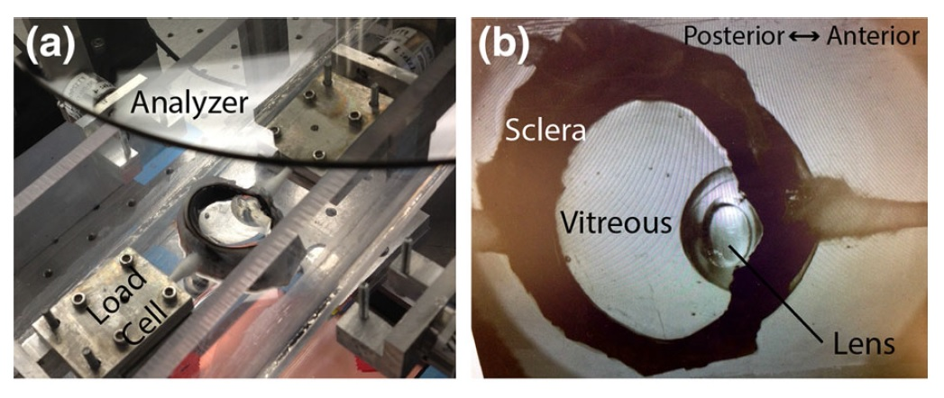
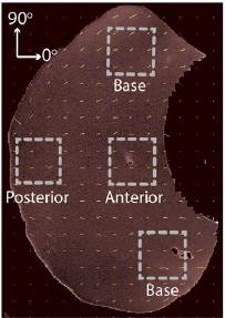
In the experiments from Shah et al. [2] fresh bovine eyes were cut in an anterior-posterior direction to create approximately 2 cm thick samples with an optically clear window to analyze the changes during the experiment, see Figure 1. Placed in an anterior-posterior orientation to the load cells the samples were attached at the sclera and near the lens by cotton swabs fixed via clamps to the load cells, Figure 1. Then the samples were uniaxially stretched by simultaneously moving both load cells in 3 mm increments (up to 12 mm) with 120 s of equilibration time between each loading step, see Figure 2. Mechanical strain was measured from sparse marker arrays on the surface of the vitreous and temporal collagen behavior was estimated from creep compliance rheological tests.

Figure 1. Experiment by Shah et al. [2]. (Reprinted by permission from Springer Customer Service Centre GmbH: Springer Nature, Annals of Biomedical Engineering, Shah et al., On the spatiotemporal material anisotropy of the vitreous body in tension and compression, © 2016.)

Figure 2. Prescribed deformation.

3.1. Geometry

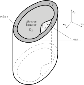
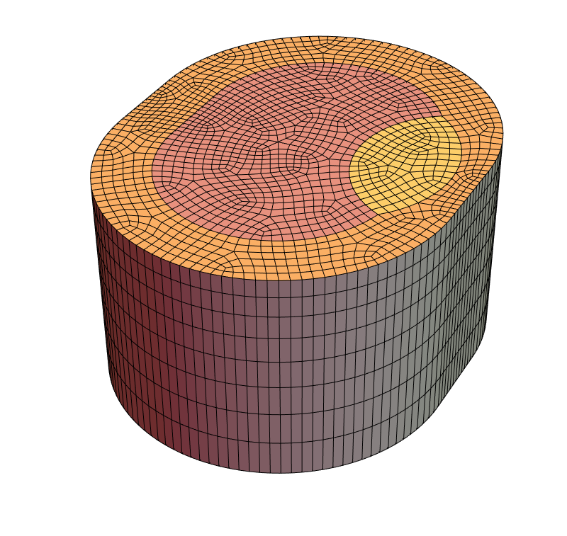
Motivated by these experiments we consider the following problem. The sample is modelled as a 2 cm high cylinder, see Figure 4a, while the cylinder cross-section has the shape similar to that in the experiment by Shah et al. [2], see Figure 3. The domain is composed of three parts, the vitreous humor occupies the cavity $\Omega_{X}$ that is formed by the lens $\Omega_{X}^{1}$ and the sclera $\Omega_{X}^{2}$, see Figure 4a. The thickness of the sclera is around 5 mm around the vitreous and the lens, the exact dimensions used for the mesh generation for the finite element method are available as a supplementary material.

Figure 3. Undeformed vitreous, Shah et al. [2]. (Reprinted by permission from Springer Customer Service Centre GmbH: Springer Nature, Annals of Biomedical Engineering, Shah et al., On the spatiotemporal material anisotropy of the vitreous body in tension and compression, © 2016.)

(a) Domain decomposition in the reference configuration – lens, sclera and vitreous humour.

(b) Surface decomposition in the reference configuration – boundary conditions.

(c) Discretization of the reference configuration using the Gmsh mesh generator, see Geuzaine and Remacle [18]; vitreous humour (red), sclera (brown), lens (yellow). Complete quantitative description of the geometry is available in the supplementary material.

Figure 4. Problem geometry.

3.2. Boundary conditions

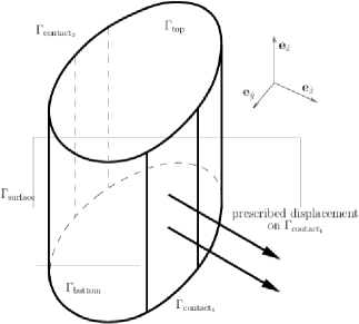
Concerning the boundary conditions, we prescribe boundary conditions that again resemble the experimental setting by Shah et al. [2]. The bottom base of the cylinder $\Gamma_{\mathrm{bottom}}$ that is placed at $z=0$, see Figure 4b, is assumed to be immovable in the direction of the $z$-axis, hence the $z$ component of the displacement vector $\bm{u}$ is fixed to zero. Further, the bottom base is allowed to move freely in the horizontal direction, hence in the direction of $x$ and $y$-axis we prescribe no-traction boundary conditions on $\bm{\varphi}(\Gamma_{\mathrm{bottom}})$, where $\bm{\varphi}$ denotes the deformation between the reference and current configuration. In total, on $\Gamma_{\mathrm{bottom}}$ we set

$$\left.\bm{u}\bullet\bm{e}_{\hat{z}}\right|_{\bm{\varphi}(\Gamma_{\mathrm{bottom}})} =0,$$ (3.1a)

$$\left.\mathbb{T}\bm{n}\bullet\bm{e}_{\hat{x}}\right|_{\bm{\varphi}(\Gamma_{\mathrm{bottom}})} =0,$$ (3.1b)

$$\left.\mathbb{T}\bm{n}\bullet\bm{e}_{\hat{y}}\right|_{\bm{\varphi}(\Gamma_{\mathrm{bottom}})} =0,$$ (3.1c)

where $$\mathbb{T} \bm{n} \Gamma_{\mathrm{top}}$$ denotes the Cauchy stress tensor, and denotes the unit outward normal in the current configuration. The top base of the cylinder is assumed to be traction free, and we set

$$\left.\mathbb{T}\bm{n}\right|_{\bm{\varphi}(\Gamma_{\mathrm{top}})}=\bm{0},$$ (3.1d)

and the same holds for the lateral walls of the cylinder,

$$\left.\mathbb{T}\bm{n}\right|_{\bm{\varphi}(\Gamma_{\mathrm{surface}})}=\bm{0}.$$ (3.1e)

On the vertical strips $$\Gamma_{\mathrm{contact}_{1}} \Gamma_{\mathrm{contact}_{2}} \Gamma_{\mathrm{contact}_{1}} \Gamma_{\mathrm{contact}_{2}} x u_{x}=_{\mathrm{def}}\bm{u}\bullet\bm{e}_{\hat{x}}$$ and we prescribe the displacement corresponding to the experiment by Shah et al. [2]. Both on the anterior part and the posterior part we prescribe the displacement in the -axis direction and we allow the sample to freely move in the other directions

$$\left.\mathbb{T}\bm{n}\bullet\bm{e}_{\hat{y}}\right|_{\bm{\varphi}(\Gamma_{\mathrm{contact}_{12}})} =0,$$ (3.1f)

$$\left.\mathbb{T}\bm{n}\bullet\bm{e}_{\hat{z}}\right|_{\bm{\varphi}(\Gamma_{\mathrm{contact}_{12}})} =0.$$ (3.1g)

On the posterior part $$\Gamma_{\mathrm{contact}_{2}} x u_{x}=0 u_{x} \Gamma_{\mathrm{contact}_{1}} 3\,\mathrm{mm} \nicefrac{{mm}}{{s}}$$ we fix the displacement in the -axis direction . The displacement on the anterior part is increased in four prolongation steps by . One prolongation step takes one second with the corresponding velocity of 3 . Together with 119 s to relax afterwards each prolongation step we have 2 min of equilibration time between each displacement step, see Figure 2 for the plot of the prescribed displacement versus time.

The exact quantitative description of locations of the surface components $\Gamma_{\mathrm{bottom}}$, $\Gamma_{\mathrm{top}}$, $\Gamma_{\mathrm{surface}}$ and $\Gamma_{\mathrm{contact}_{1}}$ and $\Gamma_{\mathrm{contact}_{2}}$ is given in the supplementary material.

4. Constitutive relations

4.1. Vitreous humour

The available experimental data, see Sharif-Kashani et al. [13], indicate that the rheological behaviour of the vitreous humour can be described by an incompressible viscoelastic Burgers-type model, whilst the usage of a complex rheological model is enforced by the presence of multiple relaxation mechanisms. The Burgers-type model is, as many viscoelastic rate-type models, see for example Wineman and Rajagopal [19], motivated by a one-dimensional mechanical spring/dashpot analogue. The one-dimensional mechanical analogue consists of two linear dashpots and two linear springs with an additional dashpot to obtain a more convenient (from the perspective of fitting the experimental data) model than the original Burgers model.

(a) Two Maxwell elements with an additional dashpot in parallel.

(b) Two Kelvin–Voigt elements with an additional dashpot in series.

Figure 5. One dimensional mechanical analogues for a Burgers-type viscoelastic model.

The first possible mechanical analogue for Burgers-type model is shown in Figure 5a. This mechanical analogue consists of two Maxwell-type elements and an additional dashpot in parallel, see Figure 5a. The one-dimensional stress-strain relation for this model has the form

$$\sigma+\left(\frac{\nu_{1}}{\mu_{1}}+\frac{\nu_{2}}{\mu_{2}}\right)\dot{\sigma}+\frac{\nu_{1}\nu_{2}}{\mu_{1}\mu_{2}}\ddot{\sigma}=\left(\nu_{1}+\nu_{2}+\mu_{3}\right)\dot{\epsilon}+\left(\frac{\nu_{1}\left(\nu_{2}+\nu_{3}\right)}{\mu_{1}}+\frac{\nu_{2}\left(\nu_{1}+\nu_{3}\right)}{\mu_{2}}\right)\ddot{\epsilon}+\frac{\nu_{1}\nu_{2}\nu_{3}}{\mu_{1}\mu_{2}}\dddot{\epsilon}$$ (4.1)

where $\sigma$ denotes the stress, $\epsilon$ denotes the strain, and the dot denotes the time derivative. Parameters $\nu_{1}$, $\nu_{2}$, $\nu_{3}$ and $\mu_{1}$, $\mu_{2}$ are material parameters characterising the elastic moduli and viscosities of the individual springs and dashpots respectively.

For numerical simulations we need to generalise the one-dimensional model into a three dimensional setting. Usually, this step is done as follows. First the Cauchy stress tensor $\mathbb{T}$ is for incompressible fluids decomposed to the pressure $p$ and the extra stress tensor $\mathbb{\widehat{\mathbb{S}}}$,

$$\mathbb{T}=-p\mathbb{I}+\mathbb{\widehat{\mathbb{S}}}.$$ (4.2a)

while the evolution equation for $$\mathbb{\widehat{\mathbb{S}}} \sigma \mathbb{\widehat{\mathbb{S}}} \dot{\epsilon} 2\mathbb{D}$$ is obtained from (4.1) by replacing by and by ,

$$\mathbb{\widehat{\mathbb{S}}}+\left(\frac{\nu_{1}}{\mu_{1}}+\frac{\nu_{2}}{\mu_{2}}\right)\accentset{\triangledown}{\mathbb{\widehat{\mathbb{S}}}}+\frac{\nu_{1}\nu_{2}}{\mu_{1}\mu_{2}}\accentset{\triangledown\!\triangledown}{\mathbb{\widehat{\mathbb{S}}}}=2\left(\nu_{1}+\nu_{2}+\mu_{3}\right)\mathbb{D}+2\left(\frac{\nu_{1}\left(\nu_{2}+\nu_{3}\right)}{\mu_{1}}+\frac{\nu_{2}\left(\nu_{1}+\nu_{3}\right)}{\mu_{2}}\right)\accentset{\triangledown}{\mathbb{D}}+2\frac{\nu_{1}\nu_{2}\nu_{3}}{\mu_{1}\mu_{2}}\accentset{\triangledown\!\triangledown}{\mathbb{D}},$$ (4.2b)

where $\mathbb{D}$ denotes the symmetric part of the velocity gradient, $\mathbb{D}=_{\mathrm{def}}\frac{1}{2}\left(\nabla\bm{v}+(\nabla\bm{v})^{\top}\right)$, and the symbol $\accentset{\triangledown}{{\mathbb{A}}}$ denotes the upper convected Oldroyd derivative

$$\accentset{\triangledown}{\mathbb{\widehat{\mathbb{S}}}}=_{\mathrm{def}}\frac{\partial{\mathbb{\widehat{\mathbb{S}}}}}{\partial{t}}+(\bm{v}\cdot\nabla)\mathbb{\widehat{\mathbb{S}}}-(\nabla\bm{v})\mathbb{\widehat{\mathbb{S}}}-\mathbb{\widehat{\mathbb{S}}}(\nabla\bm{v})^{\top}.$$ (4.3)

The second possible mechanical analogue for Burgers-type model is shown in Figure 5b. This mechanical analogue consists of two Kelvin–Voigt-type elements and the additional dashpot in series, see Figure 5b. The corresponding one-dimensional stress-strain relation reads

$$\sigma+\left(\frac{\tilde{\nu}_{1}+\tilde{\nu}_{3}}{\tilde{\mu}_{1}}+\frac{\tilde{\nu}_{2}+\tilde{\nu}_{3}}{\tilde{\mu}_{2}}\right)\dot{\sigma}+\frac{\tilde{\nu}_{1}\tilde{\nu}_{2}+\tilde{\nu}_{1}\tilde{\nu}_{3}+\tilde{\nu}_{2}\tilde{\nu}_{3}}{\tilde{\mu}_{1}\tilde{\mu}_{2}}\ddot{\sigma}=\tilde{\nu}_{3}\dot{\epsilon}+\left(\frac{\tilde{\nu}_{1}\tilde{\nu}_{3}}{\tilde{\mu}_{1}}+\frac{\tilde{\nu}_{2}\tilde{\nu}_{3}}{\tilde{\mu}_{2}}\right)\ddot{\epsilon}+\frac{\tilde{\nu}_{1}\tilde{\nu}_{2}\tilde{\nu}_{3}}{\tilde{\mu}_{1}\tilde{\mu}_{2}}\dddot{\epsilon},$$ (4.4)

where $\tilde{\nu}_{1}$, $\tilde{\nu}_{2}$, $\tilde{\nu}_{3}$ and $\tilde{\mu}_{1}$, $\tilde{\mu}_{2}$ again denote material parameters characterising the elastic moduli and viscosities of the individual springs and dashpots respectively. Application of the same approach as before leads to the following three-dimensional generalisation of the one-dimenisonal model,

$$\mathbb{\widehat{\mathbb{S}}}+\left(\frac{\tilde{\nu}_{1}+\tilde{\nu}_{3}}{\tilde{\mu}_{1}}+\frac{\tilde{\nu}_{2}+\tilde{\nu}_{3}}{\tilde{\mu}_{2}}\right)\accentset{\triangledown}{\mathbb{\widehat{\mathbb{S}}}}+\frac{\tilde{\nu}_{1}\tilde{\nu}_{2}+\tilde{\nu}_{1}\tilde{\nu}_{3}+\tilde{\nu}_{2}\tilde{\nu}_{3}}{\tilde{\mu}_{1}\tilde{\mu}_{2}}\accentset{\triangledown\!\triangledown}{\mathbb{\widehat{\mathbb{S}}}}=2\tilde{\nu}_{3}\mathbb{D}+2\left(\frac{\tilde{\nu}_{1}\tilde{\nu}_{3}}{\tilde{\mu}_{1}}+\frac{\tilde{\nu}_{2}\tilde{\nu}_{3}}{\tilde{\mu}_{2}}\right)\accentset{\triangledown}{\mathbb{D}}+2\frac{\tilde{\nu}_{1}\tilde{\nu}_{2}\tilde{\nu}_{3}}{\tilde{\mu}_{1}\tilde{\mu}_{2}}\accentset{\triangledown\!\triangledown}{\mathbb{D}}.$$ (4.5)

Constitutive relations (4.2b) and (4.5) have the same form

$$\mathbb{S}+c_{1}\accentset{\triangledown}{\mathbb{S}}+c_{2}\accentset{\triangledown\!\triangledown}{\mathbb{S}}=c_{3}\mathbb{D}+c_{4}\accentset{\triangledown}{\mathbb{D}}+c_{5}\accentset{\triangledown\!\triangledown}{\mathbb{D}}$$ (4.6)

where $c_{i}$, $i=1,\dots,5$ denote material parameters. This observation allows one to compare the different sets of material parameters, that is to express $\nu_{1}$, $\nu_{2}$, $\nu_{3}$ and $\mu_{1}$, $\mu_{2}$ in terms of $\tilde{\nu}_{1}$, $\tilde{\nu}_{2}$, $\tilde{\nu}_{3}$ and $\tilde{\mu}_{1}$, $\tilde{\mu}_{2}$ and vice versa. It suffices to solve a system of nonlinear algebraic equations of the type $\frac{\tilde{\nu}_{1}+\tilde{\nu}_{3}}{\tilde{\mu}_{1}}+\frac{\tilde{\nu}_{2}+\tilde{\nu}_{3}}{\tilde{\mu}_{2}}=\frac{\nu_{1}}{\mu_{1}}+\frac{\nu_{2}}{\mu_{2}}$ and so forth.

Moreover, the use of the Oldroyd upper convected derivative (4.3), or for that matter of any objective tensorial derivative, inherently introduces a nonlinearity into the constitutive relations, while the original one-dimensional stress-strain is given by a linear ordinary differential equation. This is potentially a dangerous step, since various nonlinear models can reduce to the same linear one-dimensional stress–strain relation, see for example Karra and Rajagopal [20] for a discussion thereof. Consequently, the choice of the right model for the three dimensional computations is not as straightforward as it may seem.

We resolve the issue of the choice of the model as follows. The one-dimensional spring/dashpot model (4.1), constructed on the basis of the mechanical analogue shown in Figure 5a, has been already successfully generalised into the three dimensional setting via a thermodynamically-based procedure introduced by Rajagopal and Srinivasa [16] for Maxwell/Oldroyd-B type models. This procedure guarantees the compatibility of the given constitutive relation with the laws of thermodynamics, and it has motivated many further theoretical as well as numerical works concerning viscoelastic rate-type fluids, see for example Rao and Rajagopal [21], Sodhi and Rao [22], Málek et al. [23], Řehoř et al. [24], Kwack et al. [25] and Hron et al. [26]. In particular, Burgers-type models constructed via the procedure have been derived and treated numerically in Tůma [27], see also Hron et al. [28], Málek et al. [29, 30] and Narayan et al. [31]. Consequently, in the ongoing numerical simulations, we prefer this well established Burgers-type model to the Burgers-type model constructed from the mechanical analogue shown in Figure 5b.

However, the values of the material parameters have been reported by Sharif-Kashani et al. [13] for the one-dimensional model (4.4), see Table 1. (Sharif-Kashani et al. [13] did not write down a fully three dimensional model.) Therefore, if we want to use the model based on the equivalent one-dimensional model (4.1), we have to first convert the set of parameters $\tilde{\nu}_{1}$, $\tilde{\nu}_{2}$, $\tilde{\nu}_{3}$ and $\tilde{\mu}_{1}$, $\tilde{\mu}_{2}$ to the set $\nu_{1}$, $\nu_{2}$, $\nu_{3}$ and $\mu_{1}$, $\mu_{2}$ via the procedure described above. This gives the parameter values reported in Table 2. In both tables the symbols $\tau_{i}$ and $\tilde{\tau}_{i}$ denote the relaxation time, that is the viscosity divided by the elastic shear modulus, $\tau_{i}=_{\mathrm{def}}\frac{\nu_{i}}{\mu_{i}}$, $i=1,2$ and $\tilde{\tau}_{i}=_{\mathrm{def}}\frac{\tilde{\nu}_{i}}{\tilde{\mu}_{i}}$, $i=1,2$.

Parameter	Description	Units	Value
$\tilde{\nu}_{3}$	viscosity	$\mathrm{Pa}\cdot\mathrm{s}$	$1.057$$\>\times\>$	$10^{3}$
$\tilde{\mu}_{1}$	first elastic shear modulus	$\mathrm{Pa}$	$1.66$$\>\times\>$	$10^{0}$
$\tilde{\mu}_{2}$	second elastic shear modulus	$\mathrm{Pa}$	$1.14$$\>\times\>$	$10^{0}$
$\tilde{\tau}_{1}$	first relaxation time	$\mathrm{s}$	$1.97$$\>\times\>$	$10^{0}$
$\tilde{\tau}_{2}$	second relaxation time	$\mathrm{s}$	$90$$\>\times\>$	$10^{0}$

Table 1. Material parameter values for the vitreous humour as reported in Sharif-Kashani et al. [13], one-dimensional model (4.4).

Parameter	Description	Units	Value		Source	Computation
$\rho$	density	$\nicefrac{\mathrm{kg}}{\mathrm{m^{3}}}$	$1.0053-1.0089$$\>\times\>$	$10^{3}$	Murphy et al. [32]	$1.007$$\>\times\>$	$10^{3}$
$\nu_{3}$	viscosity	$\mathrm{Pa}\cdot\mathrm{s}$	$2.37$$\>\times\>$	$10^{0}$	Sharif-Kashani et al. [13]	$2.37$$\>\times\>$	$10^{0}$
$\mu_{1}$	shear modulus	$\mathrm{Pa}$	$6.45$$\>\times\>$	$10^{-1}$	Sharif-Kashani et al. [13]	$6.45$$\>\times\>$	$10^{-1}$
$\mu_{2}$	shear modulus	$\mathrm{Pa}$	$8.98$$\>\times\>$	$10^{-1}$	Sharif-Kashani et al. [13]	$8.98$$\>\times\>$	$10^{-1}$
$\tau_{1}$	relaxation time	$\mathrm{s}$	$1.60$$\>\times\>$	$10^{3}$	Sharif-Kashani et al. [13]	$1.60$$\>\times\>$	$10^{3}$
$\tau_{2}$	relaxation time	$\mathrm{s}$	$25.06$$\>\times\>$	$10^{0}$	Sharif-Kashani et al. [13]	$25.06$$\>\times\>$	$10^{0}$
$\mu$	shear modulus, sclera	$\mathrm{Pa}$	$330$$\>\times\>$	$10^{3}$	Grytz et al. [33]	$330$$\>\times\>$	$10^{3}$
$\mu$	shear modulus, lens	$\mathrm{Pa}$	$0.19-59.6$$\>\times\>$	$10^{3}$	Wilde et al. [34]	$10$$\>\times\>$	$10^{3}$
$\rho$	density, sclera	$\nicefrac{\mathrm{kg}}{\mathrm{m^{3}}}$	$1.076$$\>\times\>$	$10^{3}$	Su et al. [35]	$1.05$$\>\times\>$	$10^{3}$
$\rho$	density, lens	$\nicefrac{\mathrm{kg}}{\mathrm{m^{3}}}$	$1.104$$\>\times\>$	$10^{3}$	Su et al. [35]	$1.05$$\>\times\>$	$10^{3}$

Table 2. Material parameter values for the vitreous humour, the sclera and the lens. Material parameters for Burgers-type viscoelastic model (4.2b) has been calculated from the experimental data by Sharif-Kashani et al. [13], see Table 1. Symbols $\tau_{i}$ and $\tilde{\tau}_{i}$ denote the relaxation time, that is the viscosity divided by the elastic shear modulus, $\tau_{i}=_{\mathrm{def}}\frac{\nu_{i}}{\mu_{i}}$, $i=1,2$ and $\tilde{\tau}_{i}=_{\mathrm{def}}\frac{\tilde{\nu}_{i}}{\tilde{\mu}_{i}}$, $i=1,2$. Column “Computation” shows the material parameter values used in the reported numerical simulation.

Finally, we note that in (4.2) it is convenient to introduce a decomposition

$$\mathbb{\widehat{\mathbb{S}}}=2\nu_{3}\mathbb{D}+\mathbb{S},$$ (4.7)

that allows one to rewrite (4.2) in an equivalent form as

$$\mathbb{T} =-p\mathbb{I}+2\nu_{3}\mathbb{D}+\mathbb{S},$$ (4.8a)

$$\accentset{\triangledown\!\triangledown}{\mathbb{S}}+\left(\frac{\mu_{1}}{\nu_{1}}+\frac{\mu_{2}}{\nu_{2}}\right)\accentset{\triangledown}{\mathbb{S}}+\frac{\mu_{1}\mu_{2}}{\nu_{1}\nu_{2}}\mathbb{S} =2\left(\frac{\mu_{1}\mu_{2}}{\nu_{2}}+\frac{\mu_{1}\mu_{2}}{\nu_{1}}\right)\mathbb{D}+2(\mu_{1}+\mu_{2})\accentset{\triangledown}{\mathbb{D}}.$$ (4.8b)

Using this reformulation of (4.2), it is straightforward to see that the model indeed provides a generalisation of the standard Navier–Stokes fluid model where $\mathbb{T}=-p\mathbb{I}+2\nu_{3}\mathbb{D}$.

4.2. Sclera and lens

The sclera and the lens are modelled as hyperelastic solids, see Truesdell and Noll [36], with the strain energy density $W$. Following Grytz et al. [33] the response of human sclera is described by the strain energy density in the form

$$W=\frac{1}{2}\mu\left(J^{-2/3}\operatorname{Tr}\mathbb{C}-3\right)+\frac{1}{2}\kappa(\ln J)^{2},$$ (4.9)

where $\mathbb{F}$ denotes the deformation gradient, $J=_{\mathrm{def}}\det\mathbb{F}$, and $\mathbb{C}=_{\mathrm{def}}\mathbb{F}^{\rm T}\mathbb{F}$. Parameter $\mu$ is referred to as the elastic shear modulus, while $\kappa$ is referred to as the elastic bulk modulus. Since both sclera and lens are almost incompressible, we enforce the incompressibility by taking $\kappa=1000\,\mu$ which consequently makes $J\doteq 1$, and thus $\rho\doteq\rho_{0}=const.$ Parameter values for human sclera and lens are shown in Table 2.

5. Full system of governing equations

5.1. Governing equations for the flow of vitreous humour

Vitreous humour is described by the three-dimensional Burgers-type model (4.8). Since this is a fluid-like model, it is convenient to formulate the governing equations in the Eulerian description. The balance of mass and the balance of linear momentum take the form

$$\operatorname{div}\bm{v} =0,$$ (5.1a)

$$\rho\left(\frac{\partial{\bm{v}}}{\partial{t}}+(\bm{v}\cdot\nabla)\bm{v}\right) =\operatorname{div}\mathbb{T},$$ (5.1b)

where $\bm{v}$ denotes the velocity, and where we have already exploited the fact that we are dealing with an incompressible homogenous fluid. The Cauchy stress tensor is given by (4.8).

However, formulation (4.8) is not convenient for numerical treatment. It turns out, see Tůma [27] and Hron et al. [28], that (4.8) can be rewritten as

$$\mathbb{T}=-p\mathbb{I}+2\nu_{3}\mathbb{D}+\mu_{1}(\mathbb{B}_{1}-\mathbb{I})+\mu_{2}(\mathbb{B}_{2}-\mathbb{I}),$$ (5.2a)

where the left Cauchy–Green tensors $$\mathbb{B}_{1} \mathbb{B}_{2}$$ and satisfy

$$\accentset{\triangledown}{{\mathbb{B}}_{1}}+\frac{\mu_{1}}{\nu_{1}}\left(\mathbb{B}_{1}-\mathbb{I}\right) =\mathbb{0},$$ (5.2b)

$$\accentset{\triangledown}{{\mathbb{B}}_{2}}+\frac{\mu_{2}}{\nu_{2}}\left(\mathbb{B}_{2}-\mathbb{I}\right) =\mathbb{0}.$$ (5.2c)

This form is convenient for several reasons. First, the second order differential equation (4.8b) for $\mathbb{S}$ has been replaced by two first order differential equations for $\mathbb{B}_{1}$ and $\mathbb{B}_{2}$, which simplifies time stepping algorithm. Second, quantities $\mathbb{B}_{1}$ and $\mathbb{B}_{2}$ correspond to the “state” of the springs in Figure 5a, which means that it is easy to specify the initial conditions for $\mathbb{B}_{1}$ and $\mathbb{B}_{2}$. Indeed, in the (initial) undeformed state, one has to set $\mathbb{B}_{1}=\mathbb{I}$ and $\mathbb{B}_{2}=\mathbb{I}$, see Hron et al. [28] for details.

5.2. Governing equations for the deformation of the lens and the sclera

The governing equations for the lens and sclera are formulated in the Lagrangian description. The balance of mass and linear momentum take the the form

$$\rho_{0} =J\rho,$$ (5.3a)

$$\rho_{0}\frac{\partial^{2}{\bm{u}}}{\partial{t}^{2}} =\operatorname{Div}\mathbb{P},$$ (5.3b)

where $$\rho \rho_{0} \bm{u} \mathbb{F}=\mathbb{I}+\nabla\bm{u} \mathbb{P} W$$ denotes the density in the current configuration, denotes the density in the reference configuration, and is the displacement, and denotes the deformation gradient. The symbol stands for the first Piola–Kirchhoff stress tensor, which is related to the strain energy density via the formula

$$\mathbb{P}=\frac{\partial{W}}{\partial{\mathbb{F}}},$$ (5.3c)

see for example Truesdell and Noll [36], where the specific strain energy density $$W$$ for the sclera/lens is given by (4.9).

6. Numerical solution of the fluid-structure interaction problem

The overall mechanical response of the eye stems from an interaction of the flowing vitreous humour and the deforming sclera and the lens. In our approach we aim to compute the whole problem on a fixed mesh.

The governing equations for the solid parts (5.3) are formulated in the Lagrangian description, and are solved for in the fixed reference domain $\Omega_{X}^{1}$ and $\Omega_{X}^{2}$ for the unknown displacement $\bm{u}$ and velocity field $\bm{v}$. (Symbol $\Omega_{X}^{1}$ denotes the reference domain occupied by the lens, while $\Omega_{X}^{2}$ denotes the reference domain occupied by the sclera, see Figure 4a.) On the other hand, the governing equations for the vitreous humour (5.1) are formulated in the Eulerian description, that is they hold in the domain that is at the given instant occupied by the fluid, and they must be solved for the unknowns $\bm{v}$, $p$, $\mathbb{B}_{1}$, $\mathbb{B}_{2}$. However the domain occupied by the fluid is changing in time. The problem of moving domain is addressed by the the arbitrary Lagrangian-Eulerian (ALE) method, see for example Donea et al. [17] and Scovazzi and Hughes [37], that is based on the mapping of the changing domain (moving mesh) to the fixed domain $\Omega_{\chi}$. This introduces an additional unknown – the deformation of the mesh $\hat{\bm{u}}$.

Using the ALE method, the fluid-structure interaction is computed using a monolithic approach, where all unknowns fields for the solid and fluid part are solved for simultaneously. This monolithic approach has been successfully applied in the case of interaction between a neo-Hookean solid and a Newtonian fluid in a two-dimensional setting, see for example Razzaq et al. [38], as well as in a three dimensional setting, see for example Hron and Mádlík [39].

6.1. Viscoelastic part

The governing equations for the viscoelastic fluid are mapped by ALE method to a fixed domain $\Omega_{\chi}$. In a two-dimensional setting, the Burgers-type model has been already treated by the ALE method, see Hron et al. [28]. In contrast to Hron et al. [28], here we deal with a fully three dimensional fluid-structure interaction problem, and we need to take into account the interaction with two solid materials. The ALE method leads to the following weak formulation that is used for finite element discretisation of the corresponding equations

$$\int_{\Omega_{\chi}}\hat{J}\operatorname{Tr}\left((\nabla_{\chi}\bm{v})\hat{\mathbb{F}}^{-1}\right)q\ \mathrm{d}\chi =0,$$ (6.1a)

$$\int_{\Omega_{\chi}}\hat{J}\rho\left[\frac{\partial{\bm{v}}}{\partial{t}}+(\nabla_{\chi}\bm{v})\left(\hat{\mathbb{F}}^{-1}\left(\bm{v}-\frac{\partial{\hat{\bm{u}}}}{\partial{t}}\right)\right)\right]\cdot\bm{q}\ \mathrm{d}\chi+\int_{\Omega_{\chi}}\hat{J}\hat{\mathbb{T}}\hat{\mathbb{F}}^{-\rm T}\cdot\nabla_{\chi}\bm{q}\ \mathrm{d}\chi =0,$$ (6.1b)

$$\hat{\mathbb{T}}=-p\mathbb{I}+\nu_{3}\left((\nabla_{\chi}\bm{v})\hat{\mathbb{F}}^{-1}+\hat{\mathbb{F}}^{-\rm T}(\nabla_{\chi}\bm{v})^{\rm T}\right)+\mu_{1}(\mathbb{B}_{1}-\mathbb{I})+\mu_{2}(\mathbb{B}_{2} -\mathbb{I}),$$ (6.1c)

$$\int_{\Omega_{\chi}}\hat{J}\left[\frac{\partial{\mathbb{B}_{1}}}{\partial{t}}+(\nabla_{\chi}\mathbb{B}_{1})\left(\hat{\mathbb{F}}^{-1}\left(\bm{v}-\frac{\partial{\bm{u}}}{\partial{t}}\right)\right)-(\nabla_{\chi}\bm{v})\hat{\mathbb{F}}^{-1}\mathbb{B}_{1}-\mathbb{B}_{1}\hat{\mathbb{F}}^{-\rm T}(\nabla_{\chi}\bm{v})^{\rm T}+\frac{\mu_{1}}{\nu_{1}}(\mathbb{B}_{1}-\mathbb{I})\right]\cdot\mathbb{Q}_{1}\ \mathrm{d}\chi =0,$$ (6.1d)

$$\int_{\Omega_{\chi}}\hat{J}\left[\frac{\partial{\mathbb{B}_{2}}}{\partial{t}}+(\nabla_{\chi}\mathbb{B}_{2})\left(\hat{\mathbb{F}}^{-1}\left(\bm{v}-\frac{\partial{\bm{u}}}{\partial{t}}\right)\right)-(\nabla_{\chi}\bm{v})\hat{\mathbb{F}}^{-1}\mathbb{B}_{2}-\mathbb{B}_{2}\hat{\mathbb{F}}^{-\rm T}(\nabla_{\chi}\bm{v})^{\rm T}+\frac{\mu_{2}}{\nu_{2}}(\mathbb{B}_{2}-\mathbb{I})\right]\cdot\mathbb{Q}_{2}\ \mathrm{d}\chi =0,$$ (6.1e)

$$\int_{\Omega_{\chi}}\nabla_{\chi}\hat{\bm{u}}\cdot\nabla_{\chi}\hat{\bm{t}}\ \mathrm{d}\chi =0.$$ (6.1f)

where $q,\bm{q},\mathbb{Q}_{1},\mathbb{Q}_{2},\bm{t}$ are the admissible test functions, $\hat{\bm{u}}$ is the corresponding ALE displacement, $\hat{}\mathbb{F}$ its deformation gradient $\hat{\mathbb{F}}=\mathbb{I}+\nabla_{\chi}\hat{\bm{u}}$, $\hat{J}=\det{\hat{\mathbb{F}}}$ and $\nabla_{\chi}$ denotes the gradient operator in the ALE frame. As it is apparent from the last equation, the mesh motion is governed by the equation

$$-\Delta_{\chi}\hat{\bm{u}}=\bm{0},$$ (6.2)

which is the standard choice in the ALE method. All points on the boundary $\partial\Omega_{\chi}$ are material points, thus it holds $\frac{\partial{\hat{\bm{u}}}}{\partial{t}}=\bm{v}$. This relation is enforced by employing the method of Lagrange multipliers that is based on finding the extreme points of the Lagrange function

$$L(\bm{\lambda},\hat{\bm{u}},\bm{v})=_{\mathrm{def}}\left(\frac{\partial{\hat{\bm{u}}}}{\partial{t}}-\bm{v}\right)\cdot\bm{\lambda}$$ (6.3)

where $\bm{\lambda}$ denotes the vector of Lagrange multipliers that are defined on $\partial\Omega_{\chi}$ only which does not increase a lot the size of problem. Note that (6.2) implies that $\partial\Omega_{\chi}$ is composed of material points, and thus the transformed Cauchy stress tensor $\hat{J}\hat{\mathbb{T}}\hat{\mathbb{F}}^{-\rm T}$ is, on the boundary $\partial\Omega_{\chi}$, the first Piola-Kirchhoff stress tensor.

6.2. Solid part

The governing equations for the solid parts are solved in $\Omega_{X}^{1}$ and $\Omega_{X}^{2}$, and they take the form

$$\int_{\Omega_{X}^{i}}\left(\frac{\partial{\bm{u}^{i}}}{\partial{t}}-\bm{v}^{i}\right)\cdot\bm{q}_{1}\ \mathrm{d}X =0,$$ (6.4a)

$$\int_{\Omega_{X}^{i}}\rho_{0}^{i}\frac{\partial{\bm{v}^{i}}}{\partial{t}}\cdot\bm{q}_{2}\ \mathrm{d}X+\int_{\Omega_{X}^{i}}\mathbb{P}^{i}\cdot\nabla_{X}\bm{q}_{2}\ \mathrm{d}X =0,$$ (6.4b)

where $i=1,2$, and where $\bm{q}_{1},\bm{q}_{2}$ are admissible test functions, $\bm{u}^{i}$, $\bm{v}^{i}$ and $\mathbb{P}^{i}$ denote the displacement/velocity/first Piola–Kirchhoff stress in the domain occupied by the sclera and the lens respectively, and $\rho_{0}^{i}$ denotes the reference density of the sclera and the lens respectively.

6.3. Interaction between the vitreous body, the sclera and the lens

The interaction between the solids occupying the domains $\Omega_{X}^{1}$ and $\Omega_{X}^{2}$ and the viscoelastic fluid occupying the domain $\Omega_{\chi}$ takes place on the interfaces between the domains. On the interfaces we enforce the continuity of the displacements and the stresses, that is

$$\bm{u}_{i} =\hat{\bm{u}} \mathbb{P}_{i}\bm{N} =\hat{J}\mathbb{T}\hat{\mathbb{F}}^{-\rm T}\bm{N}\quad\text{on}\ \partial\Omega_{\chi}\cap\partial\Omega_{X}^{i}\ (\text{interface\ between\ fluid\ and\ solid}),\quad i=1,2,$$ and (6.5a)

$$\bm{u}_{1} =\bm{u}_{2} \mathbb{P}_{1}\bm{N} =\mathbb{P}_{2}\bm{N}\quad\text{on}\ \partial\Omega_{X}^{1}\cap\partial\Omega_{X}^{2}\ (\text{interface\ between\ two\ solids}),$$ and (6.5b)

where $\bm{N}$ is the unit normal vector to the interface.

6.4. Implementation

Weak forms of the governing equations (5.1) and (5.3) are discretised in space using the finite element method, while the time derivatives are approximated with the backward Euler method. The three-dimensional domains $\Omega_{\chi}$, $\Omega_{X}^{1}$, $\Omega_{X}^{2}$ are approximated by $\Omega_{\chi,h}$, $\Omega_{X,h}^{1}$, $\Omega_{X,h}^{2}$ and discretised by regular hexahedra, see Figure 4c. The velocity $\bm{v}$ is approximated by $H_{1}$ elements, other unknowns $\mathbb{B}_{1}$, $\mathbb{B}_{2}$, $\bm{u}$ and $\hat{\bm{u}}$ are also approximated by $H_{1}$ elements, while the pressure $p$ is approximated by piecewise constant elements $P_{0}$.

The finite element method is implemented in the AceGen/AceFEM system Korelc [40, 41]. AceGen is a code generation system, and AceFEM is a finite element environment that uses the generated code. The provided automatic differentiation feature is used for the computation of the first Piola–Kirchhoff stress tensor (5.3c), and the exact tangent matrix used by the Newton solver to treat the non-linearities. The consequent set of linear equations is solved by conjugate gradient squared iterative solver, see Sonneveld [42], that is a part of the package Intel MKL Pardiso. The linear solver finishes when the relative residuum of the linear system reaches $10^{-4}$ and the stopping criterion for the Newton solver is $10^{-9}$.

7. Results

The numerical code introduced above has been used in solving the boundary value problem described in Section 3. In order to identify the impact of the choice of a rheological model for the vitreous humour on the response of the eye, we have solved the boundary value problem for two rheological models.

In the first numerical experiment, the vitreous humour has been described by the simple Navier–Stokes fluid model, while in the other numerical experiment we have used the Burgers-type model introduced in Section 4.1. (Note that the Navier–Stokes model corresponds to the Burgers-type model with $\mu_{1}=0$ and $\mu_{2}=0$, hence the computation for the Navier–Stokes model is just a special case of the computation for the Burgers-type model.) The comparison of these two rheological models is of interest from the practical point of view, since the Navier–Stokes rheological model corresponds to a pathological vitreous humour, while the Burgers-type model describes a healthy vitreous humour. Using the different rheological models for the vitreous humour, we have compared the quantitative and qualitative characteristics of the obtained numerical solutions.

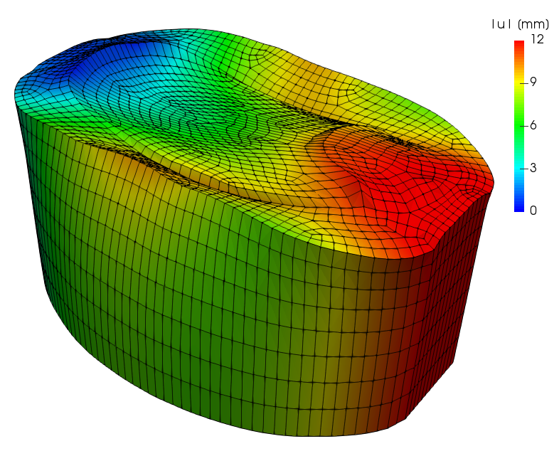
First, given the displacement of the boundary $\Gamma_{\mathrm{contact}_{1}}$, see Figure 2 and Section 3 for details, we have been interested in the overall force response and the overall displacement induced inside the eye. In particular, using the computed solution we have computed the force that is necessary to maintain the prescribed displacement of the boundary, that is

$$F_{x}=\left(-\int_{\Gamma_{\mathrm{contact}_{1}}}\mathbb{P}\bm{N}\mathrm{d}\mathrm{S}\right)\bullet\bm{e}_{\hat{x}},$$ (7.1)

and the displacement $u_{z}$ of a fictitious test particle placed at the top and in the middle of the vitreous. The overall displacement field $\bm{u}$ at the end of the test is shown in Figure 6. The plots of $F_{x}$ and $u_{z}$ are shown in Figure 7. We see that the overall force response is almost independent on the choice of the rheological model. This is an expected result, since the force response must be clearly dominated by the elastic response of the sclera and the lens. The difference between the two rheological models starts to be apparent at the level of displacement field in the vitreous humour, see Figure 7b, although the difference is relatively small.

Figure 6. Solution at $t=480\,\mathrm{s}$, displacement magnitude mapped to the current configuration.

(a) Force $F_{x}$, see (7.1), that is necessary to maintain the prescribed displacement. (Curves for the Navier–Stokes fluid and the Burgers-type fluid overlap.)

(b) Displacement $u_{z}$ of the test particle at top in the middle of the vitreous.

Figure 7. Response to the prescribed displacement of the boundary $\Gamma_{\mathrm{contact}_{1}}$, see Figure 2. Vitreous humour modelled either as the Navier–Stokes fluid of the Burgers-type viscoelastic fluid.

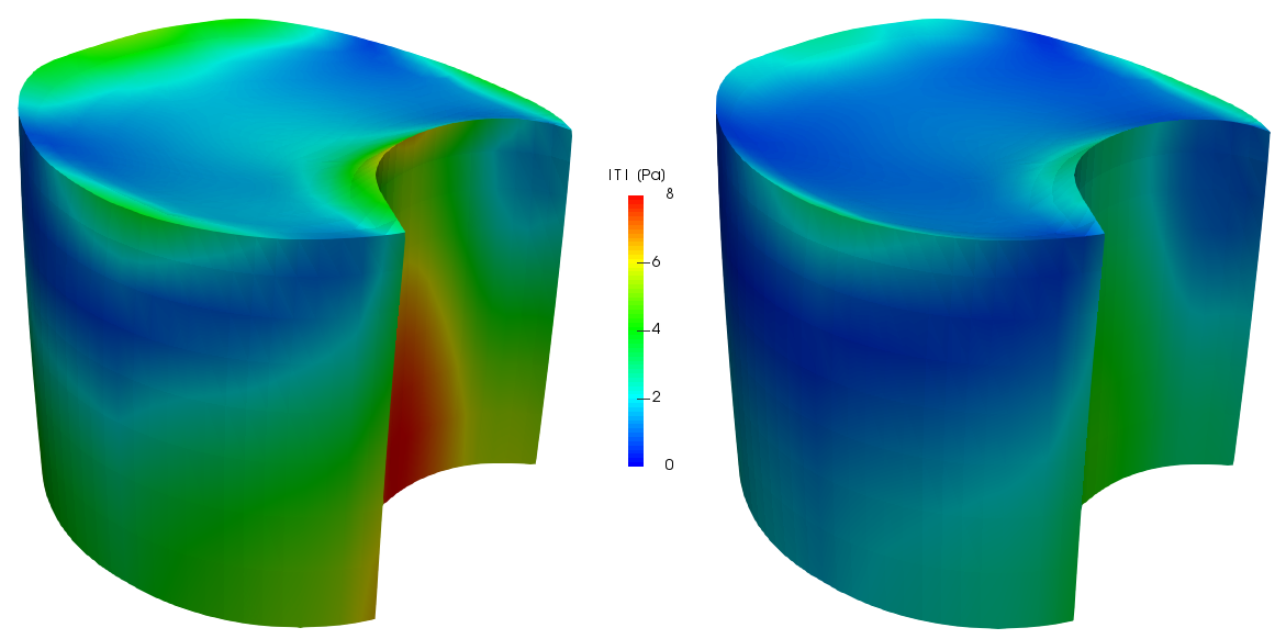
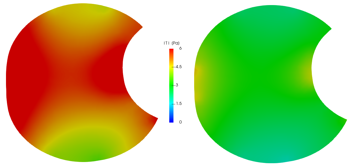
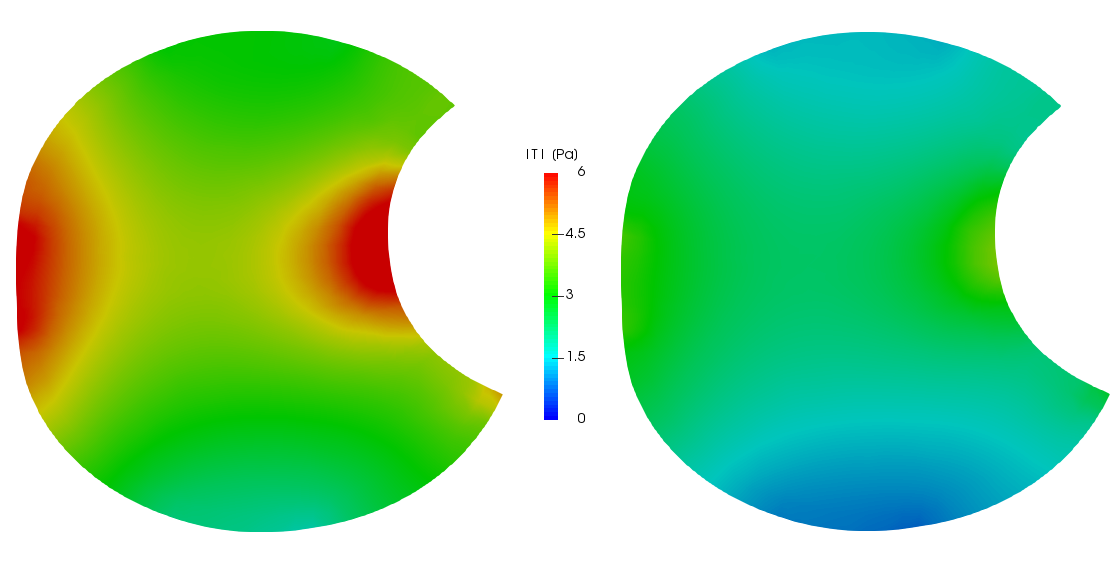
Second, given the displacement of the boundary $\Gamma_{\mathrm{contact}_{1}}$, see Figure 2 and Section 3 for details, we have been interested in the stress distribution in the vitreous humour. The magnitude of the Cauchy stress tensor $\mathbb{T}$ in the vitreous humour is shown in Figure 8. The figure shows that the stress distribution in the vitreous humour is significantly influenced by the choice of the rheological model for the vitreous humour, while the deformation of the domain occupied by the vitreous humour is almost the same. This is clearly apparent from the additional plots showing the stress distribution at given cross-sections of the domain, see Figure 9. We can notice that the magnitude of the Cauchy stress tensor can be as much as two times higher if one compares the results predicted by the Navier–Stokes model and the results predicted by the Burgers-type model.

Figure 8. Magnitude of the Cauchy stress tensor $\mathbb{T}$ at $t=120.5\,\mathrm{s}$ (half of the second prolongation), current configuration. Vitreous humour modelled using the Burgers-type viscoelastic model (left) and the standard Navier–Stokes model (right).

(a) Cross-section with the plane $z=0$.

(b) Cross-section with the plane $z=\frac{h}{2}$.

Figure 9. Magnitude of the Cauchy stress tensor $\mathbb{T}$ at $t=120.5\,\mathrm{s}$ (half of the second prolongation), current configuration, cross-section with the plane $z=0$ and $z=\frac{h}{2}$. Vitreous humour modelled using the Burgers-type viscoelastic model (left) and the standard Navier–Stokes model (right).

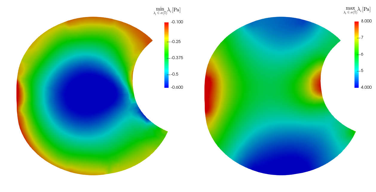
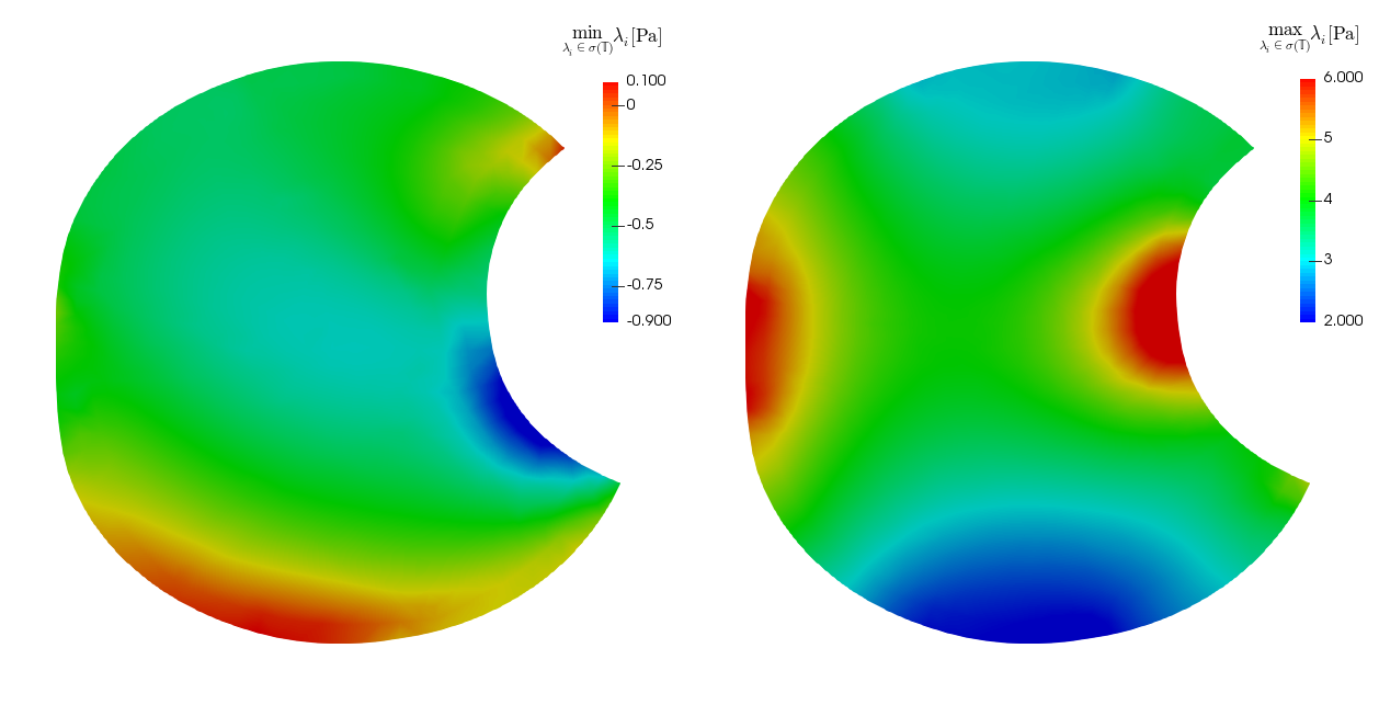
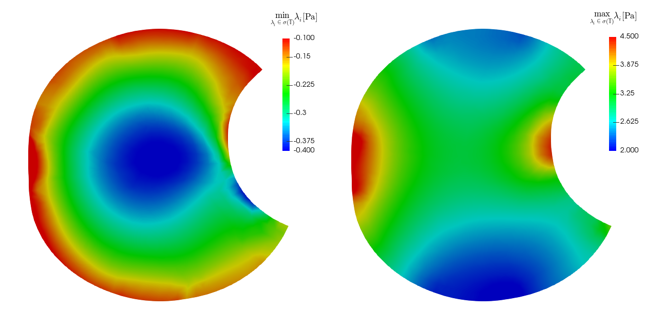
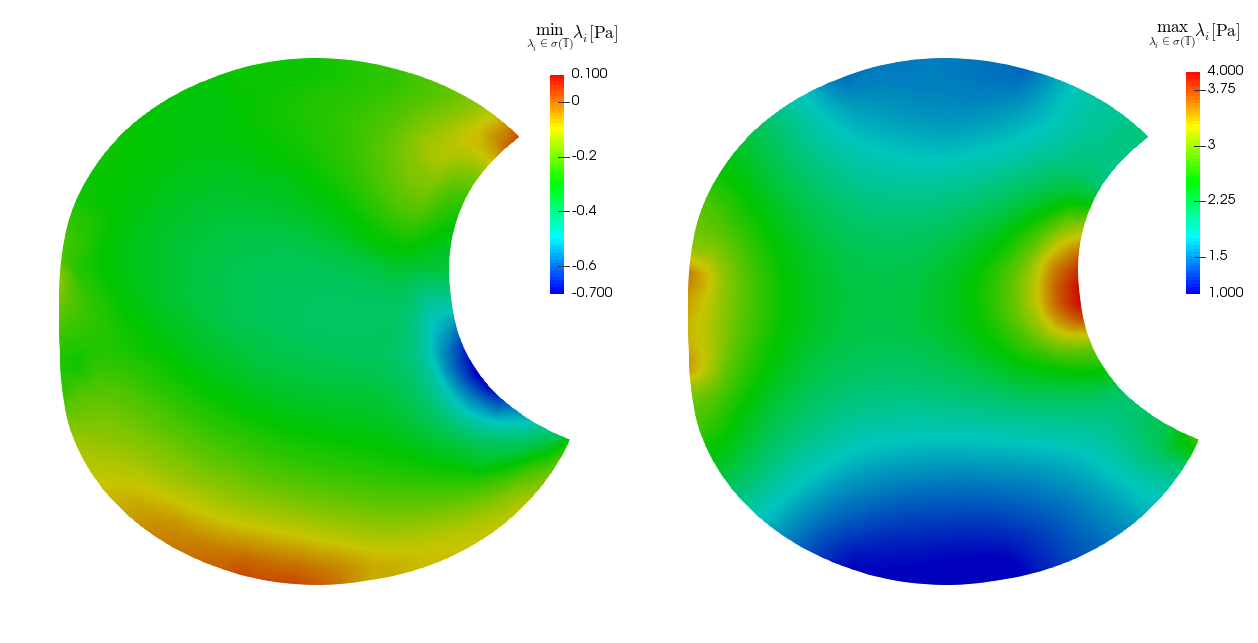
Finally, in Figures 10 and 11 we plot the spatial distribution of the minimal and maximal eigenvalues of the Cauchy stress tensor, which provides us a piece of information concerning the character of the stress at the given spatial point. (Positivity of the eigenvalue implies tension in the direction of the corresponding eigenvector, while the negativity of the eigenvalue implies compression in the direction of the corresponding eigenvector.)

(a) Cross-section with the plane $z=0$.

(b) Cross-section with the plane $z=\frac{h}{2}$.

Figure 10. Eigenvalues of the Cauchy stress tensor $\mathbb{T}$ at $t=120.5\,\mathrm{s}$ (half of the second prolongation), current configuration, cross-section with the plane $z=0$ and $z=\frac{h}{2}$. Vitreous humour modelled using the Burgers-type viscoelastic model.

(a) Cross-section with the plane $z=0$.

(b) Cross-section with the plane $z=\frac{h}{2}$.

Figure 11. Eigenvalues of the Cauchy stress tensor $\mathbb{T}$ at $t=120.5\,\mathrm{s}$ (half of the second prolongation), current configuration, cross-section with the plane $z=0$ and $z=\frac{h}{2}$. Vitreous humour modelled using the Navier-Stokes model.

8. Conclusion

A model for the deformation of an eyeball due to the application of a displacement on the surface of the eyeball has been presented. The model treats the eyeball as a cavity filled by a viscoelastic rate-type fluid (vitreous humour) that is enclosed by a hyperelastic solid (sclera, lens). The model allows one to study the motion of the vitreous humour and the displacement of the sclera and the lens, provided that the eyeball is subject to outer stimuli.

Moreover, besides the model we have also presented a numerical algorithm for solving the corresponding fluid-structure interaction problem. Since the numerical solution is based on the use of the finite element method, it in principle allows one to study the mechanical response of the eye in a patient specific geometry and in scenarios that are beyond the reach of analytical perturbation methods, see for example Ge et al. [43]. The feasibility of the proposed numerical method has been demonstrated by the solution of an initial/boundary value problem for a set of realistic parameter values in a setting that resembles the recent experiment by Shah et al. [2].

The main outcome of the trial computation is twofold. The overall flow pattern in the vitreous humour and the displacement field in the sclera and the lens seem to be, in the given scenario, not too much affected by the choice of the rheological model for the vitreous humour. On the other hand, the stress distribution in the vitreous humour and on the fluid/solid interface is very sensitive to the choice of the rheological properties of the vitreous humour. Given the fact that some eye pathologies such as retinal detachment are thought to be closely linked to mechanical processes, see Kleinberg et al. [1], the presented model can be possibly used to answer clinically relevant questions.

References

- Kleinberg et al. [2011] T. T. Kleinberg, R. T. Tzekov, L. Stein, N. Ravi, S. Kaushal, Vitreous substitutes: A comprehensive review, Survey of Ophthalmology 56 (4) (2011) 300–323, doi:10.1016/j.survophthal.2010.09.001.
- Shah et al. [2016] N. S. Shah, D. C. Beebe, S. P. Lake, B. A. Filas, On the spatiotemporal material anisotropy of the vitreous body in tension and compression, Ann. Biomed. Eng. 44 (10) (2016) 3084–3095, doi:10.1007/s10439-016-1589-3.
- David et al. [1998] T. David, S. Smye, T. Dabbs, T. James, A model for the fluid motion of vitreous humour of the human eye during saccadic movement, Phys. Med. Biol. 43 (6) (1998) 1385–1399, doi:10.1088/0031-9155/43/6/001.
- Repetto [2006] R. Repetto, An analytical model of the dynamics of the liquefied vitreous induced by saccadic eye movements, Meccanica 41 (1) (2006) 101–117, doi:10.1007/s11012-005-0782-5.
- Repetto et al. [2010] R. Repetto, J. H. Siggers, A. Stocchino, Mathematical model of flow in the vitreous humor induced by saccadic eye rotations: effect of geometry, Biomech. Model. Mechanobiol. 9 (1) (2010) 65–76, doi:10.1007/s10237-009-0159-0.
- Meskauskas et al. [2011] J. Meskauskas, R. Repetto, J. H. Siggers, Oscillatory motion of a viscoelastic fluid within a spherical cavity, J. Fluid Mech. 685 (2011) 1–22, doi:10.1017/jfm.2011.263.
- Meskauskas et al. [2012] J. Meskauskas, R. Repetto, J. H. Siggers, Shape change of the vitreous chamber influences retinal detachment and reattachment processes: Is mechanical stress during eye rotations a factor?, Invest. Ophthalmol. Vis. Sci. 53 (10) (2012) 6271–6281, doi:10.1167/iovs.11-9390.
- Bonfiglio et al. [2013] A. Bonfiglio, R. Repetto, J. H. Siggers, A. Stocchino, Investigation of the motion of a viscous fluid in the vitreous cavity induced by eye rotations and implications for drug delivery, Phys. Med. Biol. 58 (6) (2013) 1969–1982, doi:10.1088/0031-9155/58/6/1969.
- Abouali et al. [2012] O. Abouali, A. Modareszadeh, A. Ghaffariyeh, J. Tu, Numerical simulation of the fluid dynamics in vitreous cavity due to saccadic eye movement, Medical Engineering & Physics 34 (6) (2012) 681–692, doi:10.1016/j.medengphy.2011.09.011.
- Modarreszadeh and Abouali [2014] A. Modarreszadeh, O. Abouali, Numerical simulation for unsteady motions of the human vitreous humor as a viscoelastic substance in linear and non-linear regimes, J. Non-Newtonian Fluid Mech. 204 (2014) 22–31, doi:10.1016/j.jnnfm.2013.12.001.
- Repetto et al. [2014] R. Repetto, J. H. Siggers, J. Meskauskas, Steady streaming of a viscoelastic fluid within a periodically rotating sphere, J. Fluid Mech. 761 (2014) 329–347, doi:10.1017/jfm.2014.546.
- Lee et al. [1992] B. Lee, M. Litt, G. Buchsbaum, Rheology of the vitreous body. Part I: Viscoelasticity of human vitreous, Biorheology 29 (5–6) (1992) 521–533.
- Sharif-Kashani et al. [2011] P. Sharif-Kashani, J.-P. Hubschman, D. Sassoon, H. P. Kavehpour, Rheology of the vitreous gel: Effects of macromolecule organization on the viscoelastic properties, J. Biomech. 44 (3) (2011) 419–423, doi:10.1016/j.jbiomech.2010.10.002.
- Giesekus [1982] H. Giesekus, A simple constitutive equation for polymer fluids based on the concept of deformation-dependent tensorial mobility, J. Non-Newton. Fluid Mech. 11 (1-2) (1982) 69–109, doi:10.1016/0377-0257(82)85016-7.
- Burgers [1939] J. M. Burgers, Mechanical considerations – Model systems – Phenomenological theories of relaxation and viscosity, in: First report on viscosity and plasticity, chap. 1, Nordemann Publishing, New York, 5–67, 1939.
- Rajagopal and Srinivasa [2000] K. R. Rajagopal, A. R. Srinivasa, A thermodynamic frame work for rate type fluid models, J. Non-Newton. Fluid Mech. 88 (3) (2000) 207–227, doi:10.1016/S0377-0257(99)00023-3.
- Donea et al. [2004] J. Donea, A. Huerta, J.-P. Ponthot, Rodríguez-Ferrari, Arbitrary Lagrangian–Eulerian methods, in: Encyclopedia of Computational Mechanics, John Wiley & Sons, ISBN 9780470091357, doi:10.1002/0470091355.ecm009, 2004.
- Geuzaine and Remacle [2009] C. Geuzaine, J.-F. Remacle, Gmsh: A 3-D finite element mesh generator with built-in pre- and post-processing facilities, Int. J. Numer. Methods Eng. 79 (11) (2009) 1309–1331, doi:10.1002/nme.2579.
- Wineman and Rajagopal [2000] A. S. Wineman, K. R. Rajagopal, Mechanical response of polymers—an introduction, Cambridge University Press, Cambridge, 2000.
- Karra and Rajagopal [2009] S. Karra, K. R. Rajagopal, Development of three dimensional constitutive theories based on lower dimensional experimental data, Appl. Mat. 54 (2) (2009) 147–176, doi:10.1007/s10492-009-0010-z.
- Rao and Rajagopal [2002] I. J. Rao, K. R. Rajagopal, A thermodynamic framework for the study of crystallization in polymers, Z. Angew. Math. Phys. 53 (3) (2002) 365–406, doi:10.1007/s00033-002-8161-8.
- Sodhi and Rao [2010] J. S. Sodhi, I. J. Rao, Modeling the mechanics of light activated shape memory polymers, Int. J. Eng. Sci. 48 (11) (2010) 1576–1589, doi:10.1016/j.ijengsci.2010.05.003.
- Málek et al. [2015a] J. Málek, K. R. Rajagopal, K. Tůma, On a variant of the Maxwell and Oldroyd-B models within the context of a thermodynamic basis, Int. J. Non-Linear Mech. 76 (2015a) 42–47, doi:10.1016/j.ijnonlinmec.2015.03.009.
- Řehoř et al. [2016] M. Řehoř, V. Průša, K. Tůma, On the response of nonlinear viscoelastic materials in creep and stress relaxation experiments in the lubricated squeeze flow setting, Phys. Fluids 28 (10) 103102, doi:10.1063/1.4964662.
- Kwack et al. [2016] J. Kwack, A. Masud, K. R. Rajagopal, Stabilized mixed three-field formulation for a generalized incompressible Oldroyd-B model, Int. J. Numer. Meth. Fluids 83 (2016) 704–734, doi:10.1002/fld.4287.
- Hron et al. [2017] J. Hron, V. Miloš, V. Průša, O. Souček, K. Tůma, On thermodynamics of viscoelastic rate type fluids with temperature dependent material coefficients, Int. J. Non-Linear Mech. 95 (2017) 193–208, doi:10.1016/j.ijnonlinmec.2017.06.011.
- Tůma [2013] K. Tůma, Identification of rate type fluids suitable for modeling geomaterials, Ph.D. thesis, Charles University, 2013.
- Hron et al. [2014] J. Hron, K. R. Rajagopal, K. Tůma, Flow of a Burgers fluid due to time varying loads on deforming boundaries, J. Non-Newton. Fluid Mech. 210 (2014) 66–77, doi:10.1016/j.jnnfm.2014.05.005.
- Málek et al. [2015b] J. Málek, K. R. Rajagopal, K. Tůma, A thermodynamically compatible model for describing the response of asphalt binders, Int. J. Pavement Eng. 16 (4) (2015b) 297–314, doi:10.1080/10298436.2014.942860.
- Málek et al. [2016] J. Málek, K. R. Rajagopal, K. Tůma, A thermodynamically compatible model for describing asphalt binders: solutions of problems, Int. J. Pavement Eng. 17 (6) (2016) 550–564, doi:10.1080/10298436.2015.1007575.
- Narayan et al. [2016] S. P. A. Narayan, D. N. Little, K. R. Rajagopal, Modelling the nonlinear viscoelastic response of asphalt binders, Int. J. Pavement Eng. 17 (2) (2016) 123–132, doi:10.1080/10298436.2014.925621.
- Murphy et al. [2016] W. Murphy, J. Black, G. Hastings (Eds.), Handbook of Biomaterial Properties, Springer, doi:10.1007/978-1-4939-3305-1, 2016.
- Grytz et al. [2014] R. Grytz, M. A. Fazio, M. J. Girard, V. Libertiaux, L. Bruno, S. Gardiner, C. A. Girkin, J. C. Downs, Material properties of the posterior human sclera, J. Mech. Behav. Biomed. Mater. 29 (2014) 602–617, doi:10.1016/j.jmbbm.2013.03.027.
- Wilde et al. [2012] G. S. Wilde, H. J. Burd, S. J. Judge, Shear modulus data for the human lens determined from a spinning lens test, Exp. Eye Res. 97 (1) (2012) 36–48, doi:10.1016/j.exer.2012.01.011.
- Su et al. [2009] X. Su, C. Vesco, J. Fleming, V. Choh, Density of ocular components of the bovine eye, Optom. Vis. Sci. 86 (10) (2009) 1187–1195, doi:10.1097/OPX.0b013e3181baaf4e.
- Truesdell and Noll [2004] C. Truesdell, W. Noll, The non-linear field theories of mechanics, Springer, Berlin, 3rd edn., 2004.
- Scovazzi and Hughes [2007] G. Scovazzi, T. Hughes, Lecture notes on continuum mechanics on arbitrary moving domains, Tech. Rep., Technical Report SAND-2007-6312P, Sandia National Laboratories, 2007.
- Razzaq et al. [2010] M. Razzaq, J. Hron, S. Turek, Numerical simulation of laminar incompressible fluid-structure interaction for elastic material with point constraints, in: Advances in mathematical fluid mechanics, Springer, Berlin, 451–472, doi:10.1007/978-3-642-04068-9_27, 2010.
- Hron and Mádlík [2007] J. Hron, M. Mádlík, Fluid-structure interaction with applications in biomechanics, Nonlinear Anal.-Real World Appl. 8 (5) (2007) 1431–1458, doi:10.1016/j.nonrwa.2006.05.007.
- Korelc [2002] J. Korelc, Multi-language and multi-environment generation of nonlinear finite element codes, Eng. Comput. 18 (4) (2002) 312–327, doi:10.1007/s003660200028.
- Korelc [2009] J. Korelc, Automation of primal and sensitivity analysis of transient coupled problems, Comp. Mech. 44 (5) (2009) 631–649, doi:10.1007/s00466-009-0395-2.
- Sonneveld [1989] P. Sonneveld, CGS, A fast Lanczos-type solver for nonsymmetric linear systems, SIAM J. Sci. Stat. Comput. 10 (1) (1989) 36–52, doi:10.1137/0910004.
- Ge et al. [2017] P. Ge, W. J. Bottega, J. L. Prenner, H. F. Fine, On the behavior of an eye encircled by a scleral buckle, J. Math. Biol. 74 (1) (2017) 313–332, doi:10.1007/s00285-016-1015-3.