Reinforcement Learning with Wasserstein Distance Regularisation, with Applications to Multipolicy Learning

Abstract

We describe an application of Wasserstein distance to Reinforcement Learning. The Wasserstein distance in question is between the distribution of mappings of trajectories of a policy into some metric space, and some other fixed distribution (which may, for example, come from another policy). Different policies induce different distributions, so given an underlying metric, the Wasserstein distance quantifies how different policies are. This can be used to learn multiple polices which are different in terms of such Wasserstein distances by using a Wasserstein regulariser. Changing the sign of the regularisation parameter, one can learn a policy for which its trajectory mapping distribution is attracted to a given fixed distribution.

Keywords: Reinforcement Learning, Wasserstein distance

1 Introduction and Motivation

Reinforcement learning (RL) is a formalism for to modelling and solving sequential decision problems in which an agent interacts with its environment and receives a scalar reward (Suton and Barto, 1998). In recent times, deep reinforcement learning has been successfully used to solve numerous continuous and discrete control tasks, often in continuous state spaces (Mnih et al., 2015; Silver et al., 2016).

In this paper we consider the classical reinforcement learning problem of an agent that interacts with its environment while trying to maximise its cumulative reward (Burnetas and Katehakis, 1997; Kumar and Varaiya, 2015). We are interested in RL problems modeled as Markov Decision Processes (MDP) $\mathcal{M}=(\mathcal{S},\mathcal{A},\mathcal{T},R,\gamma)$ where $\mathcal{S}$ and $\mathcal{A}$ denote the state and action spaces which could be discrete or continuous, $\gamma\in(0,1]$ is the discount factor, and $\mathcal{T}$ and $R$ are the transition and reward functions respectively. The transition function $\mathcal{T}:\mathcal{S}\times\mathcal{A}\rightarrow\Delta_{\mathcal{S}}$ specifies the dynamics of the MDP and in general is assumed to be unknown. Where given any - possibly infinite- set $\mathcal{X}$, we denote by $\Delta_{\mathcal{X}}$ the set of distributions over $\mathcal{X}$. The reward function $R:\mathcal{S}\times\mathcal{A}\rightarrow\mathbb{R}$ specifies the utility gained by the agent in a given transition. In this paper we consider both finite and infinite horizon MDPs. Due to practical considerations for our experimental results we consider finite horizon problems.

In an MDP, a trajectory $\tau=(s_{0},a_{0},r_{0},s_{1},a_{1},r_{1},\cdots)$ with $s_{i}\in\mathcal{S}$, $a_{i}\in\mathcal{A}$ and $r_{i}\in\mathbb{R}$ for all $i$ is a sequence encoding the visited states, actions taken and rewards obtained during an episode of the agent’s interaction with the environment. All trajectories satisfy $\tau\in\left(\mathcal{S}\times\mathcal{A}\times\mathbb{R}\right)^{H}$, where $H$ is the MDP’s horizon. For ease of notation we set $H=\infty$ in what follows, although all our results hold for finite $H$ and also for cases when the MDPs trajectories can have variable lengths.

Any MDP $\mathcal{M}$ has a corresponding set of trajectories $\Gamma\subset\left(\mathcal{S}\times\mathcal{A}\times\mathbb{R}\right)^{\infty}$ that may be taken. In this paper we consider stochastic policies that map any state in $\mathcal{S}$ to a distribution over actions. Any policy $\pi:\mathcal{S}\rightarrow\Delta_{\mathcal{A}}$ over $\mathcal{M}$ will induce a probability measure over its space of trajectories $\Gamma$. Let $M$ be a metric space endowed with a metric $d:M\times M\rightarrow\mathbb{R}_{+}$. An embedding is a function $f:\Gamma\rightarrow M$ mapping trajectories to points in $M$. For any MDP and policy pair $(\mathcal{M},\pi)$, an embedding $f:\Gamma\rightarrow\mathbb{R}$ induces a distribution $\pi_{M}$ over $M$. Different policies will induce different measures.

The main aim of this paper is to tackle the problem of defining a similarity measure between different policies acting over the same MDP. The central contribution of this work is to propose the use of metric space embeddings for the trajectory distributions induced by a policy and use them as the basis of novel algorithms for policy attraction and policy repulsion. The principal ingredient of our proposed algorithms is the use of a computationally tractable alternative to the Wasserstein distance between the distributions induced by trajectory embeddings. The metric $d:M\times M\rightarrow\mathbb{R}_{+}$ gives us a way to quantify how much individual trajectories differ, and this in turn can be used in the framework of optimal transport (Villani, 2008) to give a measure of how different the behaviour of different policies are.

There are many reasons why we might care about how the behaviour of policies compare against each other. For example, in the control of a telecommunications network, designing for robustness is central, and promotion of diversity is a classical approach (Pióro and Medhi, 2004). A single policy may be quite heavily reliant on certain sub-structures (links, nodes, frequencies, etc.), but due to reliability issues, it may be desirable to have other policies at our disposal which perform well but which behave differently to each other. This way, there are back-up options if the parts of the network go down. That is, in learning the different policies, we wish the trajectory distributions to have a repulsive effect on each other. This becomes especially pertinent with the rise of Software Defined Networking (SDN) (Kreutz et al., 2015), which, in a nutshell, is a paradigm in which the “intelligent” components of network control (broadly speaking, the algorithms for resource allocation) are moved away from the routers into a (logically) centralised software controller. The routers become dumb but very fast machines which take their direction from the centralised controller. This present opportunities for online (Paris et al., 2016) and real-time (Allybokus et al., 2017) control, but naturally places a smaller time horizon for mitigating robustness problems.

Another motivation is the subject of the first of our experiments. Here, we wish to model an agent trying to learn to maneuver through most efficient route between designated start and end points over a hilly terrain (modelled in our experiments as a grid world (Suton and Barto, 1998)). The most efficient route(s) maybe affected by the specifics of the agent itself, merely due to the physics of the scenario (e.g., consider the difference between an off-road 4x4 vehicle and a smaller delivery pod such as those of Starship Technologies (www.starship.xyz)), so the best route for one type of agent may not be exactly the best route for another. However, they may be similar, and this motivates us to consider using a pre-existing good route to influence the learning of the agent; the trajectory distributions have an attractive effect on each other. Within our algorithm, the difference between attractive and the aforementioned repulsive effects is a change of sign in the regularisation factor of the Wasserstein term in an objective function.

Informally stated, our contributions are as follows: We present reinforcement learning algorithms for finding a policy $\pi^{*}$ where the objective function is the standard return plus regulariser that approximates the Wasserstein distance between the distribution of a mapping of trajectories induced by $\pi^{*}$ and some fixed distribution. Thus, the algorithm tries to find a good (in the standard sense) policy $\pi^{*}$ whose trajectories are different or similar to some other, fixed, distribution of trajectories.

It is clear that in the end, the aim of control is not the policy itself but the actual behaviour of the system, which in reinforcement learning is the distribution over trajectories. The Wasserstein distance, also known as the Earth-Mover Distance (EMD) (Villani, 2008; Santambrogio, 2015), exploits an underlying geometry that the the trajectories exist in, which is something that say, Kullback-Leibler (KL) or Total Variation (TV) distance don’t. This is advantageous when a relevant geometry can be defined. It is particularly pertinent to RL because different trajectories means different behaviours, and we would like to quantify how different the behaviours of two policies are in terms of how different are the trajectories that they take. For example, if $\Gamma=\{\tau_{1},\tau_{2},\tau_{3}\}$, and each of three policies $\pi_{i}$ induces Dirac on $\tau_{i}$, then in KL and TV terms, any pair of policies are just as different to each other as any other pair. However, if $\tau_{1}$ and $\tau_{2}$ are very similar in terms of behaviour (as defined by $d(f(\tau_{1}),f(\tau_{2})$), but are both very different to $\tau_{3}$, then this will not be captured by KL and TV, but will be captured by Wasserstein.

Note that whilst the above examples have the fixed distribution coming from the previously-learned policy of the first agent, this is not necessary as the algorithms merely require a distribution as an input (without any qualification on how that distribution was obtained). The usefuleness of the algorithms are, however, particularly clear when the (fixed) input distribution comes from a learned policy as in that case, the behaviours could be quite complex, and knowing a priori how to influence the learning (e.g., through reward-shaping), can be difficult, if not impossible.

2 Entropy-regularised Wasserstein Distance

Let $\mu$ and $\nu$ be two distributions with support $x_{1},\cdots,x_{k_{1}}$ and $y_{1},\cdots,y_{k_{2}}$ with $x_{i}$ and $y_{j}$ elements of a metric space $M$ for all $i,j$. The Wasserstein distance $W(\mu,\nu)$ between $P$ and $Q$ is defined as:

$$W(\mu,\nu):=\min_{\kappa\in\mathbf{K}(\mu,\nu)}\langle\kappa,C\rangle$$ (1)

Where $C\in\mathbb{R}^{k_{1}}\times\mathbb{R}^{k_{2}}$ and satisfies $C_{i,j}=d(x_{i},y_{j})$ and $\mathbb{K}(\mu,\nu)$ denotes the set of couplings - joint distributions having $\mu$ and $\nu$ as left and right marginals respectively. Computing the Wasserstein distance and optimal coupling between two distributions $\mu$ and $\nu$ can be expensive. Instead, as proposed in  Cuturi (2013), a computationally friendlier alternative can be found in the entropy regularised variation of the Wasserstein distance, which for discrete distributions takes the form:

$$W_{\rho}(\mu,\nu):=\min_{\kappa\in\mathbf{K}(\mu,\nu)}\quad\langle\kappa,C\rangle-\rho H(\kappa)$$ (2)

Here $H(\kappa)=-\sum_{i,j}\kappa_{ij}\log\kappa_{ij}$ is the entropy of the coupling $\kappa$, and $\rho>0$ is a regularisation parameter.

More generally for the case of continuous support distributions, and following Genevay et al. (2016), let $\mathcal{X}$ and $\mathcal{Y}$ be two metric spaces. Let $\mathcal{C}(\mathcal{X})$ be the space of real-valued continuous functions on $\mathcal{X}$ and let $\mathcal{M}_{+}^{1}(\mathcal{X})$ be the set of positive Radon measures on $\mathcal{X}$. Let $\mu\in\mathcal{M}_{+}^{1}(\mathcal{X})$ and $\nu\in\mathcal{M}_{+}^{1}(\mathcal{Y})$. Let $\mathbf{K}(\mu,\nu)$ be the set of couplings between $\mu,\nu$:

$$\mathbf{K}(\mu,\nu) :=\{\kappa\in\mathcal{M}^{1}_{+}(\mathcal{X}\times\mathcal{Y})\,;\,\forall(A,B)\subset\mathcal{X}\times\mathcal{Y},\kappa(A\times\mathcal{Y})=\mu(A),\kappa(\mathcal{X}\times B)=\nu(B)\}$$

That is the set of joint distributions $\kappa\in\mathcal{M}_{+}^{1}(\mathcal{X}\times\mathcal{Y})$ whose marginals over $\mathcal{X}$ and $\mathcal{Y}$ agree with $\mu$ and $\nu$ respectively. Given a cost function $c\in\mathcal{C}(\mathcal{X}\times\mathcal{Y})$, the entropy-regularised Wasserstein distance $W_{\rho}(\mu,\nu)$ between $\mu$ and $\nu$ is defined as:

$$W_{\rho}(\mu,\nu):=\min_{\kappa\in\mathbf{K}(\mu,\nu)}\int_{\mathcal{X}\times\mathcal{Y}}c(x,y)d\kappa(x,y)+\rho\mathrm{KL}(\kappa||\mu\otimes\nu)$$ (3)

where $\forall(\kappa,\xi)\in\mathcal{M}^{1}_{+}(\mathcal{X}\times\mathcal{Y})^{2}$, the KL-divergence between $\kappa$ and $\xi$ is defined by

$$\mathrm{KL}(\kappa||\xi)=\int_{\mathcal{X}\times\mathcal{Y}}\left(\log\left(\frac{\mathrm{d}\kappa}{\mathrm{d}\xi}(x,y)\right)-1\right)\mathrm{d}\kappa(x,y).$$

Here $\frac{\mathrm{d}\kappa}{\mathrm{d}\xi}(x,y)$ is the relative density of $\kappa$ with respect to $\xi$, and we define $\mathrm{KL}(\kappa||\xi)=+\infty$ if $\kappa$ doesn’t have a density with respect to $\xi$.

Note, we say the optimal coupling because the above is a strongly-convex problem, unlike the unregularised version. The algorithm in Cuturi (2013) is based on finding the dual variables of the Lagrangian by applying Sinkhorn’s matrix scaling algorithm (Sinkhorn, 1967), which is an iterative procedure with linear convergence.

Stochastic optimisation algorithms were presented in Genevay et al. (2016) for the cases where (i) $\mu,\nu$ are both discrete, (ii) when one is discrete and the other continuous, and (iii) where both are continuous. We give algorithms for all cases, but due to their similarity and lack of space, we defer all but the continuous-continuous case to the Appendix.

3 Algorithm for Continuous-Continuous Measures

Recall $M$ is a metric space and $f:\Gamma\rightarrow M$. Let $\nu$ be a fixed measure over $M$. We parameterise our policy with a vector $\theta\in\Theta$ where $\Theta$ is a parameter space. The objective is:

$$\max_{\theta\in\Theta}\,\,V(\theta)+\lambda W_{\rho}(\mu_{\theta},\nu)$$ (4)

where $V(\theta):=\mathbb{E}_{\pi_{\theta}}\left[\sum_{t\geq 0}\gamma^{t}r(s_{t},a_{t})\,|\,s_{0}\right]\equiv\mathbb{E}_{\tau\sim\pi_{\theta}}\left[R(\tau)\right]$ is the standard objective in RL, $\mu_{\theta}$ is the distribution over $M$ induced by $\pi_{\theta}$ and $\lambda\in\mathbb{R}$ is a regularisation parameter. Note: $\lambda$ can be positive or negative. If it is positive then repulsion is promoted, whilst if it is negative, then attraction is promoted.

In Genevay et al. (2016), a stochastic optimisation algorithm is presented for computing Wasserstein distance between continuous distributions. The dual formulation gives rise to test functions $(u,v)\in\mathcal{H}\times\mathcal{H}$ where $\mathcal{H}$ is a reproducing kernel Hilbert space (RKHS). The type of RKHS we will use will be generated by universal kernels (Micchelli et al., 2006), thereby allowing uniform approximability to continuous functions $u,v$.

Proposition 1 (Dual formulation (Genevay et al., 2016))

$$W_{\rho}(\mu,\nu)=\max_{u\in\mathcal{C}(\mathcal{X}),v\in\mathcal{C}(\mathcal{Y})}\int_{\mathcal{X}}u(x)d\mu(x)+\int_{\mathcal{Y}}v(y)d\nu(y)\,-\rho\int_{\mathcal{X}\times\mathcal{Y}}\exp\left\{\frac{u(x)+v(y)-c(x,y)}{\rho}\right\}d\mu(x)d\nu(y)$$

The solution $\kappa$ of problem (3) can be recovered from a solution to the above by setting $d\kappa(x,y)=\exp\left\{\frac{u(x)+v(y)-c(x,y)}{\rho}\right\}d\mu(x)d\nu(y)$.

Applying Proposition 1 with $\mathcal{X}=\mathcal{Y}=M$, we can write (4) as

$$\max_{u,v\in\mathcal{C}(M)}\,\max_{\theta\in\Theta}\,\mathbb{E}_{\tau\sim\pi_{\theta},y\sim\nu}\left[\lambda\cdot F_{\rho}(f(\tau),y,u,v)+R(\tau)\right]$$

where $F_{\rho}(x,y,u,v):=u(x)+v(y)-\rho\exp\left\{\frac{u(x)+v(y)-c(x,y)}{\rho}\right\}$.

We consider functions $u,v$ to be elements of the RKHS $\mathcal{H}$ generated by $\mathcal{K}$. If $\mathcal{K}$ is a universal kernel over $\mathcal{X}$ ($\equiv M$), the search space for $u,v$ space will be rich enough to capture $\mathcal{C}(\mathcal{X})$ (Steinwart and Christmann, 2008). Under these assumptions the $k$’th step of stochastic gradient ascent operation in the RKHS for $u,v$ takes the form:

$$(u_{k},v_{k})=(u_{k-1},v_{k-1})+\frac{\text{constant}}{\sqrt{k}}\nabla_{u,v}F_{\rho}(x,y,u,v)$$ (5)

where $(x,y)$ are sampled from the product measure of the two measures being compared, in our case, $\mu_{\theta_{k}}$ and $\nu$. The implementation via kernels is through the following result:

Proposition 2 (Genevay et al. (2016))

The iterates $(u_{k},v_{k})$ defined in (5) satisfy $(u_{k},v_{k})=\sum_{i=1}^{k}\alpha_{i}(\kappa(\cdot,x_{i}),\kappa(\cdot,y_{i}))$, where $\alpha_{i}:=\Pi_{B_{r}}\left(\frac{\text{const}}{\sqrt{i}}\left(1-\exp\left\{\frac{u_{i-1}(x_{i})+v_{i-1}(y_{i})-c(x_{i},y_{i})}{\rho}\right\}\right)\right)$, $(x_{i},y_{i})_{i=1}^{k}$ are i.i.d. samples from $\mu\otimes\nu$, and $\Pi_{B_{r}}$ is the projection on the centered ball of radius $r$. If the solutions of (1) are in $\mathcal{H}\times\mathcal{H}$ and if $r$ is large enough, then the iterates $(u_{k},v_{k})$ converge to a solution of (1).

To get Algorithm 1, we note that by standard arguments (see e.g., Sutton and Barto, 1998),

$$\nabla_{\theta}\mathbb{E}_{\tau\sim\pi_{\theta},y\sim\nu}\left[\lambda\cdot F_{\rho}(f(\tau),y,u,v)+R(\tau)\right]$$ (6)

$$=\mathbb{E}_{\tau\sim\pi_{\theta},y\sim\nu}\left[\left(\lambda u(f(\tau))-\lambda\rho\exp\left\{\frac{u(f(\tau))+v(y)-c(f(\tau),y)}{\rho}\right\}+R(\tau)\right)\cdot\sum_{t\geq 0}\nabla_{\theta}\log\pi_{\theta}(a_{t}^{(\tau)}\,|\,s_{t}^{(\tau)})\right].$$ (7)

Algorithm 1 presented below exploits Proposition 2 to perform stochastic gradient decent on the policy parameter $\theta_{i}$ by sampling as a substitute for the expectation in (7). Parameters $(\alpha^{\theta}_{i})_{i}$ define the learning rate. With each iteration, the algorithm is growing its estimate of the functions $u$ and $v$ in the RKHS and evaluating them in lines (1) and (1) using the previous samples $X_{j},Y_{j}$ to define the basis functions $\kappa(\cdot,X_{j}),\kappa(\cdot,Y_{j})$. The variable $Z$ is merely for notational convenience.

1 Input: $\theta_{0},f,M,\lambda,\rho,\nu,(\alpha^{\theta}_{i})_{i}$;

2 Initialise: $u_{0},v_{0},\theta_{0}$;

3 for $i=1,2,\ldots$ do

4       sample $\tau\sim\pi_{\theta_{i-1}}$;

5      

6      $X_{i}\leftarrow f(\tau)$;

7      

8      sample $Y_{i}\sim\nu$;

9      

10      $u_{i-1}(X_{i}):=\sum_{j=1}^{i-1}\alpha_{j}\kappa(X_{i},X_{j})$;

11      

12      $v_{i-1}(Y_{i}):=\sum_{j=1}^{i-1}\alpha_{j}\kappa(Y_{i},Y_{j})$;

13      

14      $Z\leftarrow\exp\left\{\frac{u_{i-1}(X_{i})+v_{i-1}(Y_{i})-c(X_{i},Y_{i})}{\rho}\right\}$;

15      

16      $\theta_{i}\leftarrow\theta_{i-1}+\alpha^{\theta}_{i}\cdot\left[\left(\lambda u_{i-1}(X_{i})-\lambda\rho Z+R(\tau)\right)\cdot\sum_{t\geq 0}\nabla_{\theta}\log\pi_{\theta_{i-1}}(a_{t}^{(\tau)}\,|\,s_{t}^{(\tau)})\right]$;

17      

18      $\alpha_{i}:=\frac{\text{constant}}{\sqrt{i}}\left(1-Z\right)$

Algorithm 1 Stochastic gradient for continuous measures

4 Experiments

4.1 Testing for an Attractive Scenario

We have a 7x10 gridworld with a non-negative integer “height” associated to each cell, Figure 1. An agent starts in the lower-left corner cell and there is an absorbing state on the upper-right corner cell. Each movement incurs a penalty of $-1-z$ where $z$ is the height of the cell moved to. An episode is terminated either by a time-out or reaching the absorbing state.

Figure 1: Gridworld. Darker is cheaper.

The trajectory mapping $f(\tau)$ is a probability distribution of cell visits made by $\tau$, i.e., a count is made of the number of times each cell is visited and this value is normalised by the trajectory length. Thus, $f(\tau)$ is a point in the $7\times 10-1=69$ dimensional probability simplex. We set $\nu$ to be Dirac measure on the unique optimal solution. Policy parameterisation is by radial basis functions centred on each cell.

For this set of experiments, the aim was to test the effectiveness of our algorithms with $\lambda=-1$ against policy gradient without Wasserstein regularisation (by setting $\lambda=0$). Specifically, we wanted to determine if our algorithms got better returns for a given number of episodes (i.e., iterations). In all cases, the entropy regulariser $\rho=1$. We performed three sets of experiments based on the time-out, i.e., maximum length of a trajectory before termination of an episode: 30 steps, 40 steps and 50 steps. If the agent did not reach the absorbing state before the time-out, it would get a penalty. Hence, an optimal trajectory would incur a total cost of $-15$. Each experiment consisted of 12,000 episodes and the result recorded was the return on every 100’th episode. For each time out, we ran five experiments for each of $\lambda=-1$ and $\lambda=0$. As can be seen from Figure 2, $\lambda=-1$ (blue) out-performed $\lambda=0$ (red) in general. Indeed, the former often found a (nearly) optimal policy whereas the latter often did not. Clock execution time was not hindered by $\lambda=-1$, indeed, because good policies were found more quickly, it was usually quicker to complete the experiments.

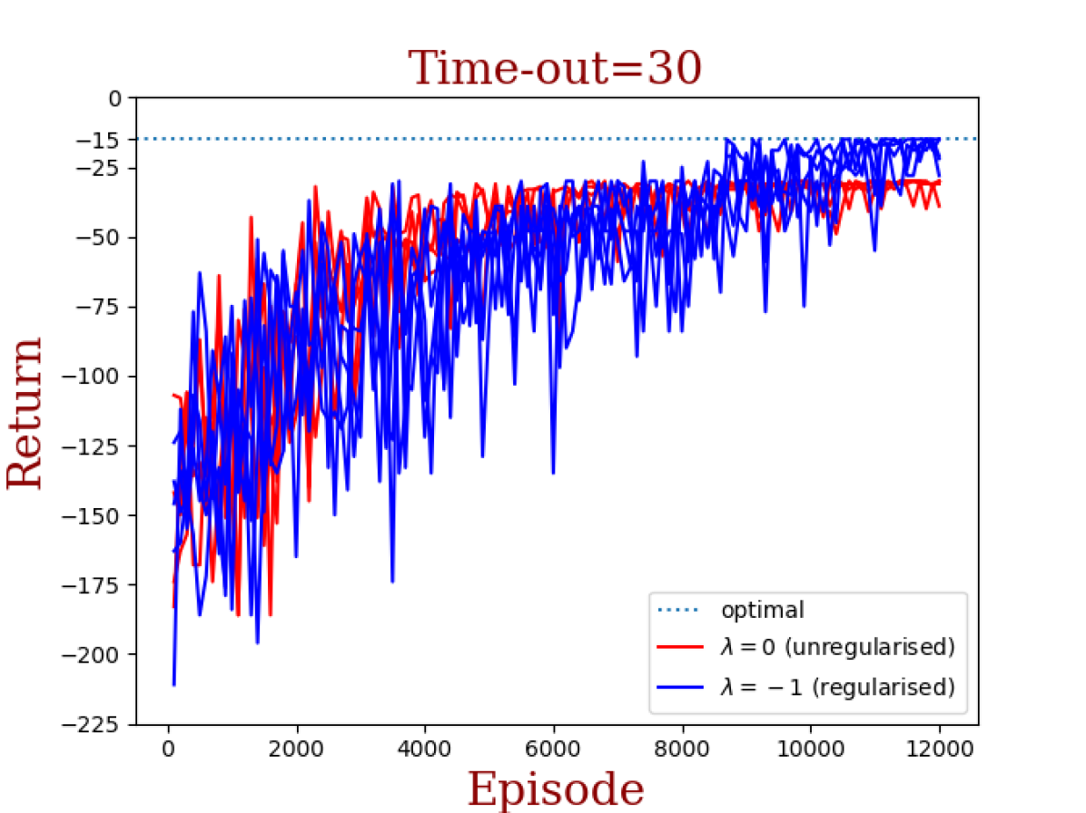
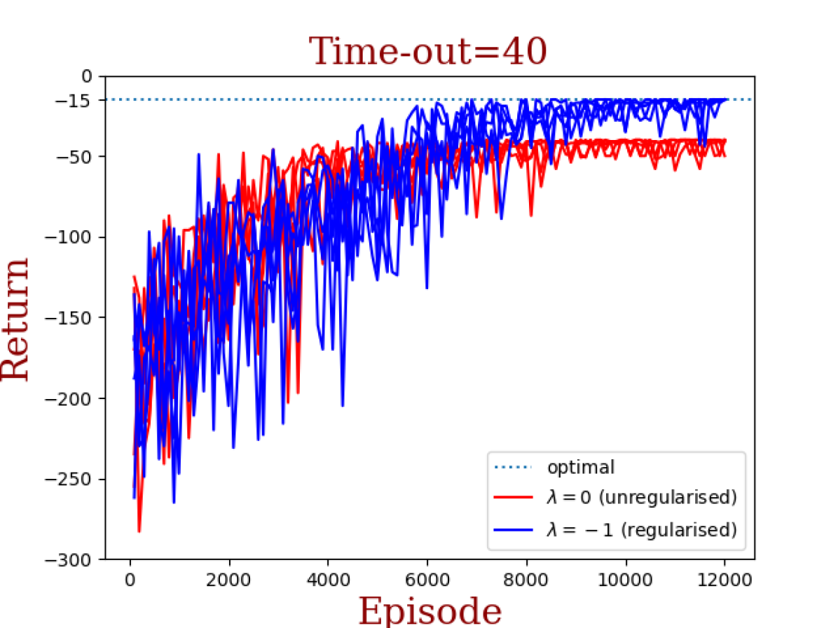
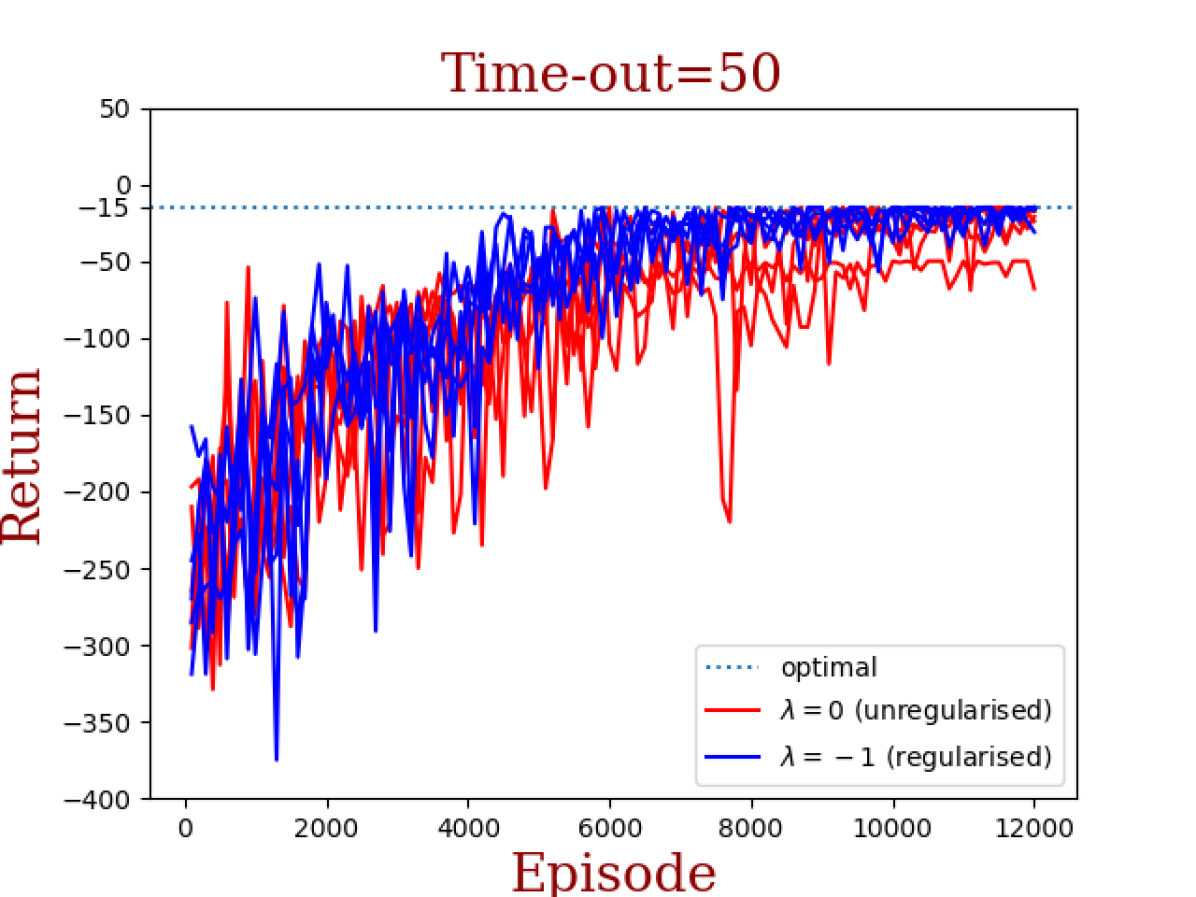
Figure 2: Attractive scenario on gridworld; regularised vs unregularised. Time-out at 30, 40 and 50 steps. Unregularised finds optimal solution more slowly or never finds it.

4.2 Testing for a Repulsive Scenario

The environment is set on a two dimensional plane where there are two goals (marked with a dot). The state space equals the $(x,y)$ positions of the agent and the reward varies in an inversely proportional way to the distance between the agent and the closest goal. The desired objective is to find the two qualitatively distinct optimal policies in an automated way. The algorithm that starts with two randomly initialized neural networks each with two hidden layers of 15 nodes each. The metric mapping is the $x$ position of the agent along the given trajectory. In contrast to the algorithms described in the previous sections, we do not start with a target distribution $\nu$ to repel at the start of the procedure. Instead, the algorithm is able to dynamically guide exploration and find two distinct policies.

The results of our runs are shown in Figure 3. Each iteration represents a policy gradient step in the parameter space of each policy. In order to compute these gradient estimates, and to find the test functions $u,v$, we use 100 rollouts of each policy in each iteration. We use $\rho=0.01$. Good convergence to two distinct policies is achieved after roughly 100 iterations. In the following plots we show, along with sample trajectories from each of the agents at a particular iteration number, images of the test functions $u,v$ and their evolution through time. It can be seen how these modify the reward structure as the algorithm runs to penalise/reward trajectories in opposing ways between the two agents. The images corresponding to iteration 15 are particularly telling as they show how even before the agents commit to a specific direction the test scores produced by our procedure strongly favour diversity.

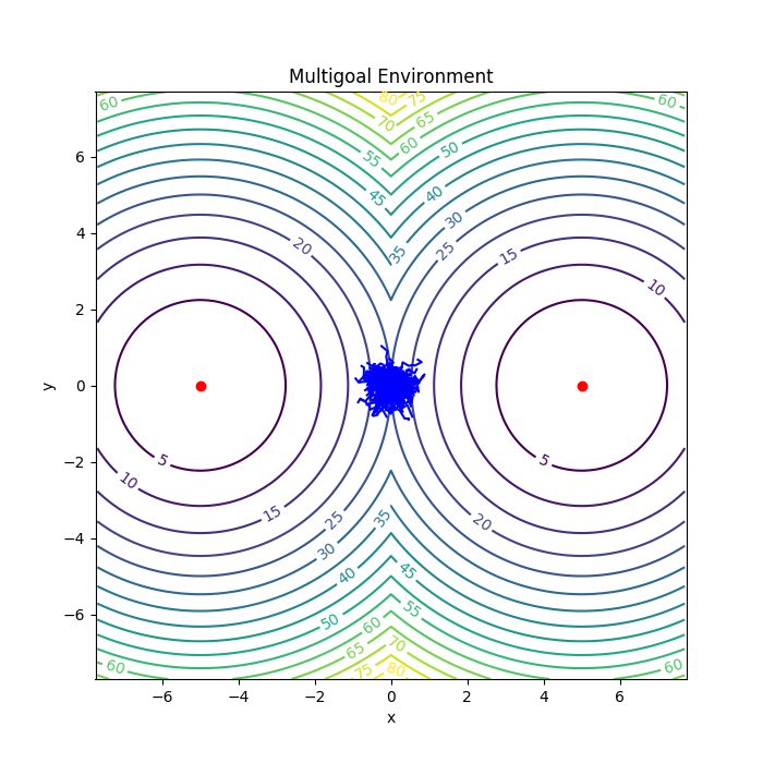
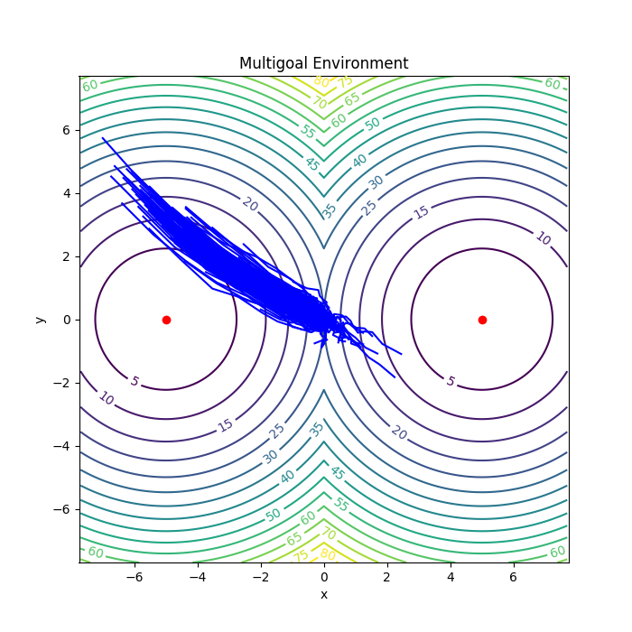
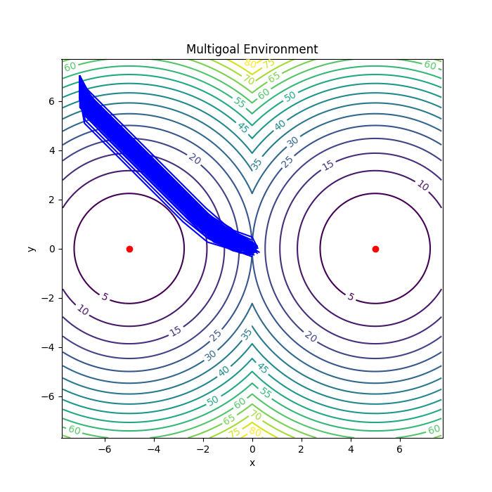
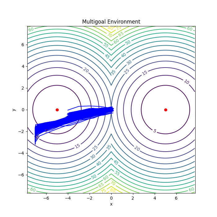
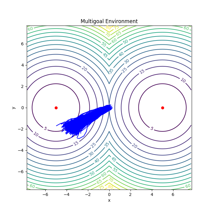
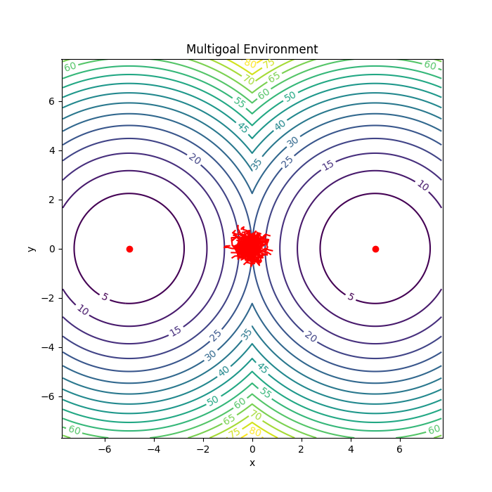
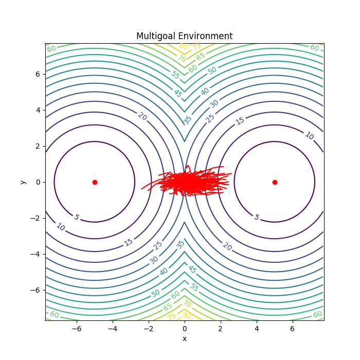
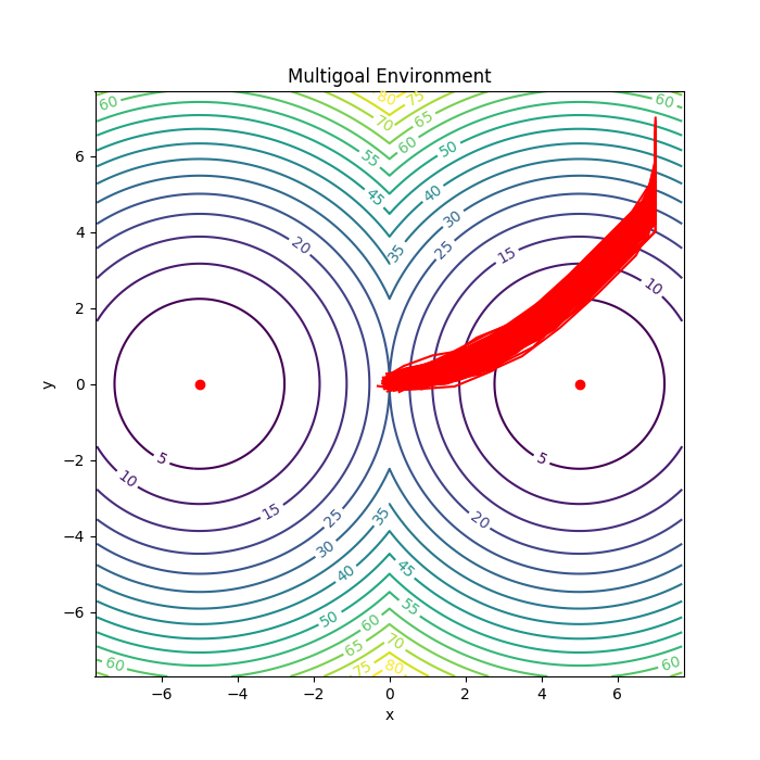
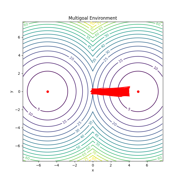
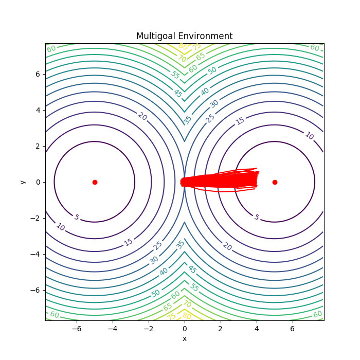
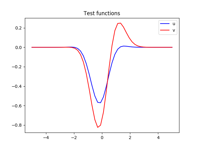
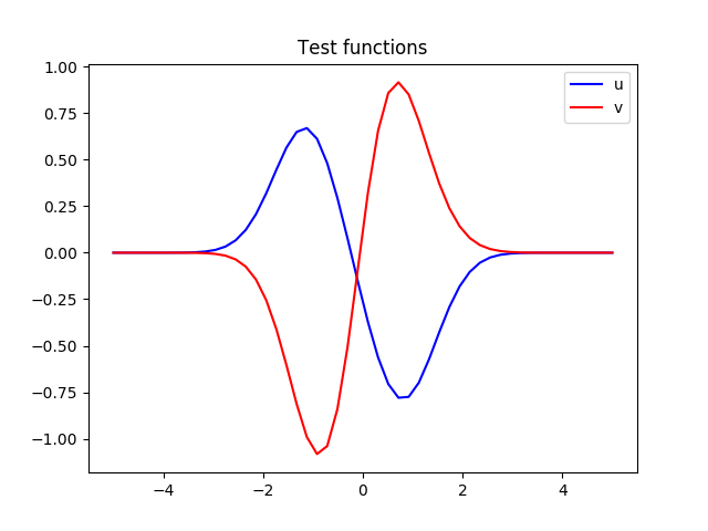
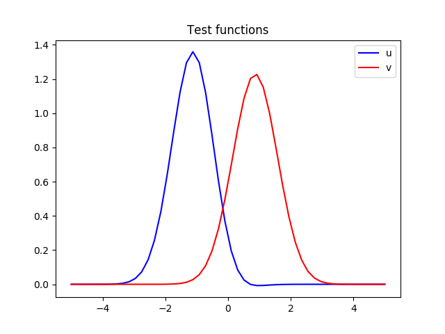
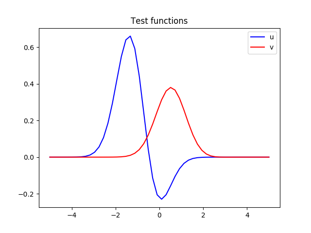
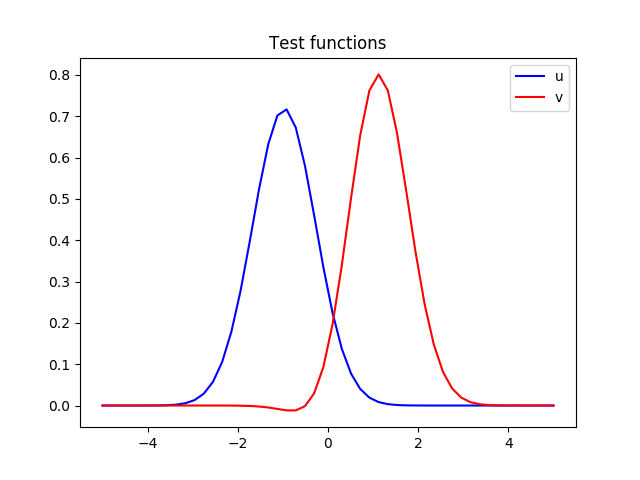
Iteration 0

Iteration 15

Iteration 30

Iteration 60

Iteration 100

Figure 3: Learning two policies by repulsive Wasserstein regularisation.

5 Conclusion, Related Work and Future Work

We have introduced the notion of Wasserstein distance regularisation into reinforcement learning as a means to quantitatively compare the trajectories (i.e., behaviours) of different policies. To the best of our knowledge, this paper is the first such example of this application. Depending on the sign of the regulariser, this technique allows policies to diverge or converge in their behaviour. This has been demonstrated through testing of algorithms presented in this paper. For future work, it would, perhaps, be natural to compare our techniques to those of imitation and inverse reinforcement learning (Abbeel and Ng, 2004; Argall et al., 2009), or techniques like guided policy search (Levine and Koltun, 2013). Direct comparison is not immediate, since our technique obliges the user to define the metric mapping, but we believe this extra demand would pay off in learning rates or through other considerations such as the flexibility it gives the user to decide what the important features of behaviour are, and tailor learning to them.

Appendix A. Wasserstein-regularised RL for (Semi-)Discrete Measures

We discuss Wasserstein distance between probability measures $\mu,\nu$. Suppose $M$ is a metric space, and $\mu=\sum_{i=1}^{n}\mu_{i}\delta_{x_{i}}$, $\nu=\sum_{j=1}^{m}\nu_{j}\delta_{y_{j}}$ are finite discrete measures where $x_{i},y_{j}\in M$. A coupling $\kappa=\kappa(\mu,\nu)$ of $\mu$ and $\nu$ is a measure over $\{x_{1},\ldots,x_{n}\}\times\{y_{1},\ldots y_{m}\}$ that preserves marginals, i.e, $\mu_{i}=\sum_{j}\kappa(\mu_{i},\nu_{j})$ $\forall i$ and $\nu_{j}=\sum_{i}\kappa(\mu_{i},\nu_{j})$ $\forall j$. This then induces a cost of “moving” the mass of $\mu$ to $\nu$, given as the (Frobenius) inner product $\langle\kappa,C\rangle$ where the matrix $C\in\mathbb{R}^{n\times m}$ has $[C]_{ij}=c_{ij}=d(x_{i},y_{j})$, i.e., the cost of moving a unit of measure from $x_{i}$ to $y_{j}$. Minimised over the space of all couplings $\mathbf{K}(\mu,\nu)$, we get the Wasserstein distance, also known as the Earth-Mover Distance (EMD) (Villani, 2008; Santambrogio, 2015).

Let $\mathbb{P}_{n}$ be the $n-1$ dimensional probability simplex. We also have a fixed distribution $\nu=(\nu_{1},\ldots,\nu_{n})\in\mathbb{P}_{n}$ over points $(y_{1},\ldots,y_{n})\in M^{n}$ i.e, with mild abuse of notation, the measure is $\mu=\sum_{j=1}^{n}\nu_{j}\delta_{y_{j}}$. Lastly, we have a cost matrix $C\in\mathbb{R}_{+}^{n\times n}$ Note $f,M,\nu,C$ are inputs to the algorithm.

Gradient-based Optimisation

Following (4) we have:

$$\nabla_{\theta}\left\{V(\theta)+\lambda W_{\rho}(\mu_{\theta},\nu)\right\}=\nabla_{\theta}V(\theta)+\lambda\nabla_{\mu}W_{\rho}(\mu,\nu)|_{\mu=\mu_{\theta}}\cdot\nabla_{\theta}\mu_{\theta}$$

Per the standard policy gradient approach (Sutton and Barto, 1998), we can sample trajectories to get an unbiased estimate of $\nabla_{\theta}V(\theta)$. Indeed, for any function $g:\Gamma\rightarrow\mathbb{R}$,

$$\nabla_{\theta}\mathbb{E}_{\tau\sim\pi_{\theta}}\left[g(\tau)\right]=\mathbb{E}_{\tau\sim\pi_{\theta}}\left[g(\tau)\,\sum_{t\geq 0}\nabla_{\theta}\log\pi_{\theta}(a_{t}\,|,\,s_{t})\right],$$ (8)

meaning we can sample trajectories to obtain unbiased estimates of $\nabla_{\theta}\mu_{\theta}$.

Finally, the term $\nabla_{\mu}W_{\rho}(\mu,\nu)|_{\mu=\mu_{\theta}}$ can be dealt with using the Sinkhorn algorithm itself: In the computation of $W_{\rho}(\mu,\nu)$ for a given pair $\mu,\nu$, the algorithm computes their optimal dual variables $u^{*},v^{*}$, respectively. It can do so because, as mentioned above, the entropy-regularisation makes the optimisation strongly convex and strong duality is exhibited. Then $u^{*}$ is a (sub)gradient of $W_{\rho}(\mu,\nu)$ with respect to $\mu$ (this will be discussed further below). Thus, given an estimate of $\mu_{\theta}$, we can estimate $\nabla_{\mu}W_{\rho}(\mu,\nu)|_{\mu=\mu_{\theta}}$.

Putting it all together, we have derived a simple stochastic gradient algorithm. In Algorithm 2, $(\alpha_{i})_{i}$ is a learning rate.

1 Input: $\theta_{0},f,M,\lambda,\rho,\nu,(\alpha_{i})_{i}$;

2 Initialise: $\theta_{0}$;

3 for $i=1,2,\ldots$ do

4       sample $\tau\sim\pi_{\theta_{i-1}}$;

5       compute estimate $gtv(\tau)$ of $\nabla_{\theta}V(\theta)|_{\theta=\theta_{i-1}}$ using (8);

6       compute estimate $gtm(\tau)$ of $\nabla_{\theta}\mu_{\theta}|_{\theta=\theta_{i-1}}$ using (8);

7       update estimate $\hat{\mu_{\theta}}$ of $\mu_{\theta}$ using $\tau$;

8       compute estimate $gtw$ of $\nabla_{\mu}W_{\rho}(\mu,\nu)|_{\mu=\mu_{\theta_{i-1}}}$ using Sinkhorn  Cuturi (2013) and $\hat{\mu_{\theta}}$;

9       $\theta_{i}\leftarrow\theta_{i-1}+\alpha_{i}\cdot\left(gtv(\tau)+\lambda\cdot gtw\cdot gtm(\tau)\right)$

Algorithm 2 Wasserstein RL for finite discrete measures

Stochastic Alternating Optimisation via Dual Formulation

The dual of the primal problem (2) was studied in Cuturi and Doucet (2014). Applying it, we get the following equivalent of (4):

$$\max_{\theta\in\Theta}\,\max_{u,v\in\mathbb{R}^{n}}\,\lambda\left(\langle u,\mu_{\theta}\rangle+\langle v,\nu\rangle-\rho B(u,v)\right)+V(\theta)$$ (9)

where

$$B(u,v):=\sum_{i,j}\exp\left\{\frac{u_{i}+v_{j}-c_{ij}}{\rho}\right\}.$$

Swapping the order of maximisations:

$$\max_{u,v\in\mathbb{R}^{n}}\,\lambda\left(\langle v,\nu\rangle-B(u,v)\right)+\max_{\theta\in\Theta}\,\lambda\langle u,\mu_{\theta}\rangle+V(\theta).$$

The term $\langle u,\mu_{\theta}\rangle$ is an expectation, and the above can be re-written:

$$\max_{u,v\in\mathbb{R}^{n}}\,\lambda\left(\langle v,\nu\rangle-B(u,v)\right)+\max_{\theta\in\Theta}\mathbb{E}_{\tau\sim\pi_{\theta}}\left[\lambda u(f(\tau))+R(\tau)\right]$$

for an appropriate function $u$.

An iterative algorithm can proceed by alternatively fixing $u,v$ and maximising $\theta$, and vice versa. When $u$ is fixed, we can apply policy gradient (Sutton and Barto, 1998) to the term $\mathbb{E}_{\tau\sim\pi_{\theta}}\left[\lambda u(f(\tau))+R(\tau)\right]$;

$$\nabla_{\theta}\mathbb{E}_{\tau\sim\pi_{\theta}}\left[\lambda u(f(\tau))+R(\tau)\right]=\mathbb{E}_{\tau\sim\pi_{\theta}}\left[\left(\lambda u(f(\tau))+R(\tau)\right)\cdot\sum_{t\geq 0}\nabla_{\theta}\log\pi_{\theta}(a_{t}^{(\tau)}\,|\,s_{t}^{(\tau)})\right]$$

Thus, sampling a trajectory from $\pi_{\theta}$ and using it to compute the bracketed term in (Stochastic Alternating Optimisation via Dual Formulation) gives an unbiased estimate of the true gradient. This can be used to update $\theta$. Further, observe that fixing $\theta$, the expression to be maximised in (9) is differentiable in $u,v$. This provides the means to increase $u,v$. This iterative alternating maximisation procedure is summarised in Algorithm 3.

1 Input: $\theta_{0},f,M,\lambda,\rho,\nu,(\alpha^{\theta}_{i})_{i},(\alpha^{u}_{i})_{i},(\alpha^{v}_{i})_{i}$;

2 Initialise: $u_{0},v_{0},\theta_{0}$;

3 for $i=1,2,\ldots$ do

4       sample $\tau\sim\pi_{\theta_{i-1}}$;

5       $\theta_{i}\leftarrow\theta_{i-1}+\alpha^{\theta}_{i-1}\cdot\left[\left(\lambda u_{i-1}(f(\tau))+R(\tau)\right)\cdot\sum_{t\geq 0}\nabla_{\theta}\log\pi_{\theta_{i-1}}(a_{t}^{(\tau)}\,|\,s_{t}^{(\tau)})\right]$;

6       $u_{i}\leftarrow u_{i-1}+\alpha_{i}^{u}\cdot\lambda\cdot\left(f(\tau)-\nabla_{u}B(u,v)|_{u=u_{i-1},v=v_{i-1}}\right)$;

7       sample $Y\sim\nu$;

8       $v_{i}\leftarrow v_{i-1}+\alpha_{i}^{v}\cdot\lambda\cdot\left(Y-\nabla_{v}B(u,v)|_{u=u_{i-1},v=v_{i-1}}\right)$

Algorithm 3 Stochastic gradient for finite discrete measures, dual formulation

The advantage of this algorithm is that the distributions $\mu_{\theta}$ and $\nu$ do not need to be represented explicitly, they only have to be sampled from.

The above can be generalised to the case $\mu$ is an arbitrary measure $\nu=\sum_{j=1}^{m}\nu_{j}\delta_{y_{j}}$ remains discrete. Starting with the form of the Wasserstein distance given in (3) (which is slightly different to the version defined in (2)), and taking $\nu$ as discrete, it was shown in Genevay et al. (2016) that by writing first-order optimality conditions, one gets:

$$W_{\rho}(\mu,\nu)=\max_{v\in\mathbb{R}^{m}}\mathbb{E}_{X\sim\mu}\left[h(X,v)\right]$$

where

$$h(x,v):=\langle v,\nu\rangle-\rho\log\left(\sum_{j=1}^{m}\exp\left\{\frac{v_{j}-c(x,y_{j})}{\rho}\right\}\nu_{j}\right).$$

Thus, in our case, we would have $f(\tau)\sim\pi_{\theta}$ in place of $X\sim\mu$ above, and our objective would be

$$\max_{\theta}\,\,V(\theta)+\lambda\max_{v\in\mathbb{R}^{m}}\mathbb{E}_{f(\tau)\sim\pi_{\theta}}\left[h(f(\tau),v)\right]=\max_{\theta}\max_{v\in\mathbb{R}^{m}}\,\,+\mathbb{E}_{f(\tau)\sim\pi_{\theta}}\left[R(\tau)+\lambda h(f(\tau),v)\right].$$

Because of the structure of $\nabla_{u}h(u,v)$, we cannot use a sampled vector $Y\sim\nu$ as we did with Algorithm 3, we have to access each element in the vector $\nu$. Hence, this algorithm is useful when $m$ is not too large. With that said, we can use incremental alternating gradient ascent, as summarised in Algorithm 4.

1 Input: $\theta_{0},f,M,\lambda,\rho,\nu,(\alpha^{\theta}_{i})_{i},(\alpha^{v}_{i})_{i}$;

2 Initialise: $v_{0},\theta_{0}$;

3 for $i=1,2,\ldots$ do

4       sample $\tau\sim\pi_{\theta_{i-1}}$;

5       $\theta_{i}\leftarrow\theta_{i-1}+\alpha^{\theta}_{i}\cdot\left[\left(\lambda h_{\rho}(f(\tau),v_{i-1})+R(\tau)\right)\cdot\sum_{t\geq 0}\nabla_{\theta}\log\pi_{\theta_{i-1}}(a_{t}^{(\tau)}\,|\,s_{t}^{(\tau)})\right]$;

6       $v_{i}\leftarrow v_{i-1}+\alpha_{i}^{v}\cdot\lambda\cdot\nabla_{v}h(x,v)|_{x=f(\tau),v=v_{i-1}}$

Algorithm 4 Stochastic gradient for discrete $\nu$, arbitrary $\mu_{\theta}$

References

- Abbeel and Ng (2004) Pieter Abbeel and Andrew Y Ng. Apprenticeship learning via inverse reinforcement learning. In Proceedings of the twenty-first international conference on Machine learning, page 1. ACM, 2004.
- Allybokus et al. (2017) Zaid Allybokus, Konstantin Avrachenkov, Jérémie Leguay, and Lorenzo Maggi. Real-time fair resource allocation in distributed software defined networks. In Teletraffic Congress (ITC 29), 2017 29th International, volume 1, pages 19–27. IEEE, 2017.
- Argall et al. (2009) Brenna D Argall, Sonia Chernova, Manuela Veloso, and Brett Browning. A survey of robot learning from demonstration. Robotics and autonomous systems, 57(5):469–483, 2009.
- Burnetas and Katehakis (1997) Apostolos N Burnetas and Michael N Katehakis. Optimal adaptive policies for markov decision processes. Mathematics of Operations Research, 22(1):222–255, 1997.
- Cuturi (2013) Marco Cuturi. Sinkhorn distances: Lightspeed computation of optimal transport. In Advances in neural information processing systems, pages 2292–2300, 2013.
- Cuturi and Doucet (2014) Marco Cuturi and Arnaud Doucet. Fast computation of wasserstein barycenters. In International Conference on Machine Learning, pages 685–693, 2014.
- Genevay et al. (2016) Aude Genevay, Marco Cuturi, Gabriel Peyré, and Francis Bach. Stochastic optimization for large-scale optimal transport. In Advances in Neural Information Processing Systems, pages 3440–3448, 2016.
- Kreutz et al. (2015) Diego Kreutz, Fernando MV Ramos, Paulo Esteves Verissimo, Christian Esteve Rothenberg, Siamak Azodolmolky, and Steve Uhlig. Software-defined networking: A comprehensive survey. Proceedings of the IEEE, 103(1):14–76, 2015.
- Kumar and Varaiya (2015) Panqanamala Ramana Kumar and Pravin Varaiya. Stochastic systems: Estimation, identification, and adaptive control, volume 75. SIAM, 2015.
- Levine and Koltun (2013) Sergey Levine and Vladlen Koltun. Guided policy search. In International Conference on Machine Learning, pages 1–9, 2013.
- Micchelli et al. (2006) Charles A Micchelli, Yuesheng Xu, and Haizhang Zhang. Universal kernels. Journal of Machine Learning Research, 7(Dec):2651–2667, 2006.
- Mnih et al. (2015) Volodymyr Mnih, Koray Kavukcuoglu, David Silver, Andrei A Rusu, Joel Veness, Marc G Bellemare, Alex Graves, Martin Riedmiller, Andreas K Fidjeland, Georg Ostrovski, et al. Human-level control through deep reinforcement learning. Nature, 518(7540):529–533, 2015.
- Paris et al. (2016) Stefano Paris, Jeremie Leguay, Lorenzo Maggi, Moez Draief, and Symeon Chouvardas. Online experts for admission control in sdn. In Network Operations and Management Symposium (NOMS), 2016 IEEE/IFIP, pages 1003–1004. IEEE, 2016.
- Pióro and Medhi (2004) Michal Pióro and Deep Medhi. Routing, flow, and capacity design in communication and computer networks. Elsevier, 2004.
- Santambrogio (2015) Filippo Santambrogio. Optimal transport for applied mathematicians. Birkäuser, NY, 2015.
- Silver et al. (2016) David Silver, Aja Huang, Chris J Maddison, Arthur Guez, Laurent Sifre, George Van Den Driessche, Julian Schrittwieser, Ioannis Antonoglou, Veda Panneershelvam, Marc Lanctot, et al. Mastering the game of go with deep neural networks and tree search. Nature, 529(7587):484–489, 2016.
- Sinkhorn (1967) Richard Sinkhorn. Diagonal equivalence to matrices with prescribed row and column sums. The American Mathematical Monthly, 74(4):402–405, 1967.
- Steinwart and Christmann (2008) Ingo Steinwart and Andreas Christmann. Support vector machines. Springer Science & Business Media, 2008.
- Suton and Barto (1998) RS Suton and AG Barto. Reinforcement learning: An introduction. cambridge, massachusetts: A bradford book, 1998.
- Sutton and Barto (1998) Richard S Sutton and Andrew G Barto. Reinforcement learning: An introduction, volume 1. MIT press Cambridge, 1998.
- Villani (2008) Cédric Villani. Optimal transport: old and new, volume 338. Springer Science & Business Media, 2008.