SSH model with long-range hoppings: topology, driving and disorder

Abstract

The Su-Schrieffer-Heeger (SSH) model describes a finite one-dimensional dimer lattice with first-neighbour hoppings populated by non-interacting electrons. In this work we study a generalization of the SSH model including longer-range hoppings, what we call the extended SSH model. We show that the presence of odd and even hoppings has a very different effect on the topology of the chain. On one hand, even hoppings break particle-hole and sublattice symmetry, making the system topologically trivial, but the Zak phase is still quantized due to the presence of inversion symmetry. On the other hand, odd hoppings allow for phases with a larger topological invariant. This implies that the system supports more edge states in the band’s gap. We propose how to engineer those topological phases with a high-frequency driving. Finally, we include a numerical analysis on the effect of diagonal and off-diagonal disorder in the edge states properties.

• January 2018

1 Introduction

One of the main tasks condensed matter physics deals with is the understanding of phases of matter. Traditionally, phase transitions were characterised following Landau’s prescription, in terms of an order parameter. Then, the discovery of new phases of matter that did not break any symmetry, nor could be characterised by the usual order parameters, lead to the appearance of topology in condensed matter systems. This new scenario emerged from the merging of physics and topology, and on a more subtle order that lies in the mathematical properties of the electronic wavefunctions. Experimentally, the first developments happened in the study of phase transitions in 2D electronic systems, which displayed a quantised Hall conductance [1]. Then, the discovery of the fractional QHE [2] and of the Spin Hall insulator in HgTe quantum wells [3] lead to the large variety of systems displaying topological properties that have been discovered so far.

Systems with non-trivial topological properties are changing the way electronics is developing. In particular, the discovery of materials with insulating bulk and metallic edges, which are also robust under a wide range of perturbations, will allow for important advances in spintronics [4], magnetism [5] or even further, to the development of topological quantum computers [6, 7, 8, 9]. Understanding how these materials behave in realistic situations is crucial, and the study of the classical toy models with new terms is of the utmost relevance. This work is framed within this context.

The starting point of this study is a canonical model of a 1D topological insulator: the Su-Schrieffer-Heeger (SSH) model [10]. It is a tight-binding model for non-interacting, spinless electrons confined in a dimer chain. It has been extensively studied both theoretically and experimentally [11, 12].

In this work, we analyze the effect of adding arbitrarily long-range hoppings to the SSH model, what we call hereafter the extended SSH model. By examining the symmetries that are preserved or broken in the resulting system, we can conclude that the presence of even and odd hopping terms has different implications on the topological properties. Hoppings to even neighbours break particle-hole and chiral (also known as sublattice) symmetries, but under certain constraints we are able to find gapped configurations with edge states. On the other hand, odd neighbours do not break any fundamental symmetries of the chain, allowing for the appearance of larger values of the topological invariant. More concretely, we study in detail the case with first- and second-neighbour hoppings, as well as first-, second- and third-neighbour hoppings.

We also discuss the feasibility of larger winding number configurations by including an AC driving field. This allows to tune the hopping amplitudes into unconventional configurations. Furthermore, we examine the effect of diagonal and off-diagonal disorder in the previous results. From the topological point of view, diagonal disorder breaks sublattice symmetry, and therefore affects the topological protection, while off-diagonal disorder maintains this symmetry.

The paper is organized as follows: In section 2 we introduce the extended SSH model; in section 3 we include a characterization of its topological properties, considering some relevant concrete examples. Section 4 presents an analysis on the effect of an AC driving field on the system, studying several drives with different shapes; in section 5 we study different types of disorder and check their effect on the edge states of the system. Finally, in section 6 we present our conclusions.

2 Extended SSH model

The Hamiltonian of the dimer chain with hoppings up to $N^{th}$-neighbours is given by:

$$H_{N}=\sum_{|i-j|\leq N}J_{ij}c^{\dagger}_{i}c_{j}+\mathrm{H.c.}\,,\quad J_{ij}=J^{*}_{ij}=J(|x_{i}-x_{j}|)\,,$$ (1)

where $c^{\dagger}_{i}$ creates a fermion in the $i^{th}$ site of the chain, and $J_{ij}=J_{ji}$ is the hopping amplitude connecting the $i^{th}$ and the $j^{th}$ sites. We can group all the sites in two sublattices $A$ and $B$. All the sites with odd indices belong to sublattice $A$ and all the sites with even indices belong to sublattice $B$ (see figure 1 for a schematic). If we restrict the model to nearest-neighbours only ($N=1$), we recover the original SSH model.

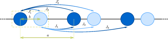
Figure 1: Dimer chain with arbitrarily long-ranged hoppings. For clearness, only hoppings to first, second and third neighbour atoms have been depicted. The unit cell length will be set to $a=1$ hereafter without loss of generality. The intracell parameter is $b$.

We assume hopping amplitudes are decaying functions of the distance between sites and define $n=|i-j|$ as the range of the corresponding hopping $J_{ij}$. Hoppings are denoted as odd or even according to their range. It is important to note that in the case of odd hoppings, for any $n\in\mathbb{N}_{\mathrm{odd}}$ and site $i$, the $(i+n)^{th}$ and $(i-n)^{th}$ sites are located at different distances. On the contrary, for even hoppings, all sites are located at the same distance for any $n\in\mathbb{N}_{\mathrm{even}}$. For the sake of simplicity, we will use the following notation from now on

$$\eqalign{J_{2i-n,2i}\equiv J_{n}\,,\quad J_{2i,2i+n}\equiv J^{\prime}_{n}\,,\quad n\in\mathbb{N}_{\mathrm{odd}}\\ J_{i,i\pm n}\equiv J_{n}\,,\quad n\in\mathbb{N}_{\mathrm{even}}}$$ (2)

For a translationally-invariant system, the Hamiltonian is block-diagonal in the momentum-space basis. Transforming $c_{2j-1}=\frac{1}{\sqrt{M}}\sum_{k}e^{ikj}a_{k}$ and $c_{2j}=\frac{1}{\sqrt{M}}\sum_{k}e^{ikj}b_{k}$, for $j=1,\dots,M$ ($M$ is the number of unit cells in the chain), we can express the Hamiltonian in Equation (1) with periodic boundary conditions as $H_{N}=\sum_{k}\Psi_{k}^{\dagger}\mathcal{H}_{N}\left(k\right)\Psi_{k}$, where we have defined $\Psi_{k}=\left(a_{k},b_{k}\right)^{T}$. The bulk momentum-space Hamiltonian $\mathcal{H}_{N}\left(k\right)$ is a $2\times 2$ matrix with the following structure: even hoppings contribute to diagonal elements, whereas odd hoppings appear in off-diagonal ones,

$$\mathcal{H}_{N}=\sum_{p}\left(\begin{array}[]{cc}2J_{2p}\cos\left(pk\right)&J^{\prime}_{2p-1}e^{ik(p-1)}+J_{2p-1}e^{-ikp}\\ J^{\prime}_{2p-1}e^{-ik(p-1)}+J_{2p-1}e^{ikp}&2J_{2p}\cos\left(pk\right)\end{array}\right)\,,$$ (3)

with $p$ ranging from $1$ to $N/2$ if $N$ is even, or $(N+1)/2$ if $N$ is odd. $\mathcal{H}_{N}$ can be written in the basis of the Pauli matrices $\vec{\sigma}=\{\sigma_{x},\sigma_{y},\sigma_{z}\}$ and the identity $\mathbf{1}$ as $\mathcal{H}_{N}=d_{0}(k)\mathbf{1}+\vec{d}(k)\cdot\vec{\sigma}$. The vector $\vec{d}(k)$ is called the Bloch vector, and its components are

$$d_{0}(k)=\sum_{p}2J_{2p}\cos(pk)\,,$$ (4)

$$d_{x}(k)=\sum_{p}\left[J^{\prime}_{2p-1}\cos\big{(}(p-1)k\big{)}+J_{2p-1}\cos(pk)\right]\,,$$ (5)

$$d_{y}(k)=\sum_{p}\left[J_{2p-1}\sin(pk)-J^{\prime}_{2p-1}\sin\big{(}(p-1)k\big{)}\right]\,,$$ (6)

$$d_{z}(k)=0\,.$$ (7)

The dispersion relation takes the form $E_{\pm}(k)=d_{0}(k)\pm|\vec{d}(k)|$, where “$+$” and “$-$” correspond to the conduction and valence band, respectively. Importantly, the fact that even hoppings of a given range $n$ have the same value in both sublattices makes $d_{z}(k)=0$.

3 Topology in extended SSH models

For one-dimensional topological insulators, the topological invariant that characterizes different topological phases is the Zak phase $\mathcal{Z}$. Equivalently, they can be characterized by the winding of the Bloch vector around the origin as $k$ varies across the first Brillouin zone. This quantity $\mathcal{W}$ is well-defined only when the Bloch vector lays in a plane containing the origin. Both are related to each other as $\mathcal{Z}=\pi\mathcal{W}\ \mathrm{mod}\ 2\pi$. Owing to the bulk-edge correspondence, the bulk topology manifests itself in presence or absence of edge states in a finite system. The number of pairs of edge states a system supports corresponds to $|\mathcal{W}|$. The winding number can be calculated in terms of the Bloch vector components (see A).

The Zak phase is a gauge invariant quantity and as such can be measured [13]. Apart from the SSH model of polyacetylene [10], the Zak phase has also been used to characterized linearly conjugated diatomic polymers [14], photonic systems [15, 16], acoustic systems [17], and recently, water wave states [18].

In the standard SSH model, the winding number can only take two values depending on the ratio between first-neighbour hopping amplitudes: $\mathcal{W}=0$ (trivial phase) if $J^{\prime}_{1}/J_{1}>1$, and $\mathcal{W}=1$ (non-trivial phase) if $J^{\prime}_{1}/J_{1}<1$. Furthermore, since there are only first-neighbour hoppings in the model, it possesses particle-hole symmetry along with time-reversal symmetry and chiral (sublattice) symmetry. Therefore, it belongs to the one-dimensional BDI class of the Atland-Zirnbauer classification of topological insulators and superconductors [19], which admits an infinite number of distinct topological phases.

In the extended SSH model the presence of even hoppings breaks particle-hole as well as chiral symmetry, changing the system Hamiltonian from BDI class to the AI class, which is trivial in 1D. Two clarifications must be made to this statement. First, for sufficiently small even hoppings this model supports edge states in the band’s gap, despite the absence of the aforementioned symmetries. Second, even hoppings preserve space-inversion symmetry when chosen as detailed in equation (1), which ensures that the winding number is still well-defined. Mathematically, terms proportional to the identity matrix (included in $d_{0}$), do not change the eigenstates, and therefore the parallel transport, i.e. the Berry connection, is unaffected. However, the presence of even hoppings does affect the energy bands and the energy levels of a finite system. They may lead to the disappearance of the edge states into the bulk bands without the corresponding change in the winding number, contrary to the expectation for a true topological phase transition. Thus, in general, there is not a one-to-one correspondence between the topological invariant and the number of edge states pairs supported by the chain as long as even hoppings are present, as shown in figure 2.

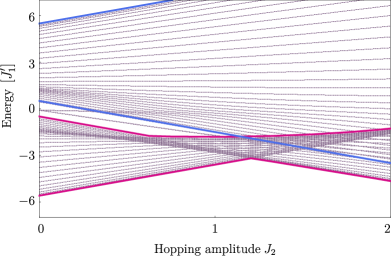
Figure 2: Spectrum for a finite system of $M=30$ and $N=3$, with $J_{1}=2J^{\prime}_{1}$, $J^{\prime}_{3}=0.5J^{\prime}_{1}$, and $J_{3}=2J^{\prime}_{1}$, as a function of $J_{2}$. The blue and fuchsia lines represent the maximum and minimum value for the conduction and valence band, respectively. First- and third-neighbour hoppings are chosen such that the system has $\mathcal{W}=2$, i.e., with two pairs of edge states. Second-neighbour alter the energy spectrum, taking the system to a metallic phase because of the overlapping of the two bands. In the gapped phase, note the different behaviour of each pair of edge states. However, the winding number is the same regardless of the value of the hopping amplitude $J_{2}$. This means that the one-to-one correspondence between $\mathcal{W}$ and the number for edge states is broken.

Regarding long-range odd hoppings, they preserve all the symmetries of the standard SSH model, and permit larger values of the topological invariant. For a given $N$, the maximum winding number possible is $\mathcal{W}_{\mathrm{max}}=\lfloor(N+1)/2\rfloor$, which is also the maximum number of pairs of edge states supported by the chain. However, one difficulty for obtaining these phases with larger invariant is that long-range hopping amplitudes must be chosen in a specific way. We will show in next section how we can achieve this by applying ac driving fields.

In the following lines we will examine in detail two different configurations.

3.1 First and second neighbour hoppings

We now study in more detail the effect of even hoppings by considering the case of first- and second-neighbour hoppings. As explained before, the study of the topology of the system requires the analysis of both bulk and edge properties.

3.1.1 Bulk physics

The momentum-space Hamiltonian in (3) takes the form

$$\mathcal{H}_{2}=\left(\begin{array}[]{cc}2J_{2}\cos\left(k\right)&J^{\prime}_{1}+J_{1}e^{-ik}\\ J^{\prime}_{1}+J_{1}e^{ik}&2J_{2}\cos\left(k\right)\end{array}\right),$$ (8)

whereas Bloch’s vector changes to:

$$d_{0}\left(k\right) = 2J_{2}\cos\left(k\right)\,,$$ (9)

$$d_{x}\left(k\right) = J^{\prime}_{1}+J_{1}\cos\left(k\right)\,,\quad d_{y}\left(k\right)=J_{1}\sin\left(k\right)\,,\quad d_{z}\left(k\right)=0\,$$ (10)

and the energy dispersion is given by $E_{\pm}\left(k\right)=2J_{2}\cos\left(k\right)\pm\sqrt{J_{1}^{{}^{\prime}2}+J_{1}^{2}+2J^{\prime}_{1}J_{1}\cos\left(k\right)}$. This expression makes clear that second-neighbour hoppings break particle-hole symmetry, which translates into an assymetric band structure about $E=0$. Still, the specific value of $J_{2}$ is of utmost importance, as the system properties change drastically. We can distinguish two regimes (see figure 3):

1. When $J_{2}<J^{\prime}_{1}/2$ and $J^{\prime}_{1}/J_{1}>1$ ($\mathcal{W}=0$) or $J_{2}<J_{1}/2$ and $J^{\prime}_{1}/J_{1}<1$ ($\mathcal{W}=1$), the system has insulating properties. This regime corresponds to a gapped phase in which the winding number is still defined by the ratio $J^{\prime}_{1}/J_{1}$ and has a one-to-one correspondence with the number of edge states. It is also significant that the direct gap turns into an indirect gap at $J_{2}=J_{1}/2$ (trivial phase), or $J_{2}=J^{\prime}_{1}/2$ (topological phase), which means that the minimum energy in the conduction band and the maximum energy in the valence band occur at different values of $k$.

2. When $J_{2}\geq J^{\prime}_{1}/2$ and $J^{\prime}_{1}/J_{1}>1$ or $J_{2}\geq J{}_{1}/2$ and $J^{\prime}_{1}/J_{1}<1$, the behaviour is expected to be metallic. In this regime the gap is indirect, but the maximum of the valence band (at $k=0$) is equal or greater to the minimum of the conduction band (at $k=\pi$). This means that the energy bands overlap without crossing, which signals the absence of a topological phase transition.

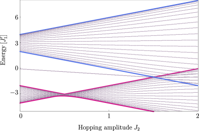
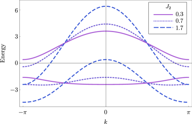
Figure 3: Effect of second-neighbour hoppings on the band structure and energy levels of a finite system. Top: Spectrum for a finite system of $M=20$ and $N=2$, with $J_{1}=2J^{\prime}_{1}$, as a function of $J_{2}$. The blue and fucsia lines represente the maximum and minimum value for the conduction and valence band, respectively. For $J_{2}<1$, the system has two edge states within the band gap. Their energy decreases as $J_{2}$ is increased until they penetrate the bulk bands for $J_{2}\geq J^{\prime}_{1}$. Also, the gap goes from direct to indirect at $J_{2}=0.5J^{\prime}_{1}$ (see main text, section 3.1.1). In the metallic phase, the bands overlap without crossing. Bottom: Bulk band structure for different values of $J_{2}$, given the previous SSH hoppings. Note how particle-hole symmetry is gradually lost as $J_{2}$ is increased, which is reflected in the loss of symmetry about $E=0$ in the energy spectrum. It is also important to notice that the case with $J_{2}=0.3J^{\prime}_{1}$ has a direct gap, with both the minimum of the conduction band and the maximum of the valence band occur at $k=\pi$. However, for $J_{2}=0.7J^{\prime}_{1}$, the gap is indirect (the minimum of the conduction band occurs at $k=\pm\pi$ and the maximum of the valence band at $k=0$). This corresponds to case (i) discussed in the previous section. On the other hand, the maximum of the valence band is greater than the minimum of the conduction band for the configuration with $J_{2}=1.7J^{\prime}_{1}$, although the bands never touch. This is an example of band structure of a system in regime (ii), when the system is expected to have metallic properties.

3.1.2 Edge physics

The topological phase of the SSH chain is characterized by the appearance of two edge modes. If the thermodynamic limit ($M\rightarrow\infty$), edge states will be degenerate at $E=0$, each of them being exponentially located at either the right of left end of the chain. If not, a small splitting of the order of $(J^{\prime}_{1}/J_{1})^{N}$ is expected [20]; edge states hybridize and become an even and odd superposition of the states located at one of the ends. The presence of chiral symmetry, represented by the operator $\mathcal{C}$, ensures that these hybridized edge states have symmetric energies about $E=0$, since they are chiral partners of each other: $|\mathrm{edge_{o}}\mathcal{i}=\mathcal{C}|\mathrm{edge}_{\mathrm{e}}\mathcal{i}\rightarrow E_{\mathrm{o}}=-E_{\mathrm{e}}$, where e and o stands for even and odd parity, respectively. By solving the dispersion relation we get that edge states have associated a complex $k=\pi+i\zeta_{\mathrm{SSH}}$, where $\zeta_{\mathrm{SSH}}$ is the inverse of the localization length. The value of $\zeta_{\mathrm{SSH}}$ is a function of the ratio $J^{\prime}_{1}/J_{1}$ [21]

$$\frac{J^{\prime}_{1}}{J_{1}}\approx e^{-\zeta_{\mathrm{SSH}}}\,.$$ (11)

When second-neighbour hoppings are added, we find the following changes in the behaviour of the edge states:

1. The absence of chiral symmetry implies that $|\mathrm{edge_{o}}\mathcal{i}=\mathcal{C}|\mathrm{edge}_{\mathrm{e}}\mathcal{i}$ does not hold anymore (see figure 4).

   

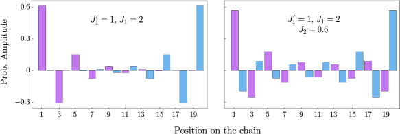
   Figure 4: Wave functions of the hybridized edge states (even parity) of a chain with $M=10$ unit cells, with:
   Left: only first-neighbour hoppings, $J_{1}=2J^{\prime}_{1}$. Edge states in the SSH chain fulfill $|\mathcal{h}\mathrm{edge_{\mathrm{o}}|\mathcal{C}|}\mathrm{edge}_{\mathrm{e}}\mathcal{i}|=1$.
   Right: first- and second-neighbour hoppings, $J_{1}=2J^{\prime}_{1}$ and $J_{2}=0.6J^{\prime}_{1}$. The presence of $J_{2}$ breaks chiral symmetry, and hence $|\mathcal{h}\mathrm{edge_{\mathrm{o}}|\mathcal{C}|}\mathrm{edge}_{\mathrm{e}}\mathcal{i}|=0.8<1$. This quantity becomes smaller as $J_{2}$ is increased.

2. The edge states energy moves away from zero as $J_{2}$ increases. Using numerical analysis, we find that the energy of both edge states varies linearly with $J_{2}$ according to

   $$E=E_{\mathrm{edge}}-2J_{2}\frac{J^{\prime}_{1}}{J_{1}}\,,$$ (12)

   where $E_{\mathrm{edge}}$ is the energy of the edge states in the SSH chain ($J_{2}=0$). This expression holds until the enery bands overlap.

3. Interestingly, we find that the addition of $J_{2}$ modifies the localization length of the edge states, which become less localized as $J_{2}$ is increased. First, knowing that the energy of the edge states depends linearly on $J_{2}$ as shown in equation (12), we can solve the dispersion relation, obtaining a expression for the $k$ associated with the edge states in terms of the hopping amplitudes

   $$k=\pm\arccos(\alpha),\,\alpha=-\frac{J^{\prime}_{1}}{J_{1}}+\frac{J_{1}J^{\prime}_{1}}{4J_{2}^{2}}-\frac{1}{4J_{2}^{2}}\sqrt{4J_{2}^{2}(J_{1}^{2}-J_{1}^{{}^{\prime}2})+J_{1}^{2}J_{1}^{{}^{\prime}2}}\,.$$ (13)

   In order for the state to be localized, we search for a solution $k$ of the form $k=\pi\pm i\zeta$, where $\zeta=1/\lambda_{\mathrm{loc}}$. If we rewrite the previous equation as $\cos(k)=\cos(\pi+i\zeta)=-\cosh(\zeta)=\alpha$, we can give an analytic expression for $\zeta$

   $$\zeta=\frac{1}{\lambda_{\mathrm{loc}}}=\mathrm{arccosh}\left(-\alpha\right)\,.$$ (14)

   In the limit $J_{2}\rightarrow J_{1}/2$ (when the bands overlap and the edge states penetrate the energy bands), for which $\zeta\rightarrow 0$. In the limit $J_{1}\rightarrow J^{\prime}_{1}$, i.e. one-dimensional atomic chain, (when the band gap is closed and the system has metallic behaviour), $\zeta\rightarrow 0$ independently of the value of $J_{2}$. In both cases, localized behaviour is lost, which agrees with the analytic and numerical results previously obtained.

   As can be seen in figure 5, $\zeta$ is affected differently by $J_{2}$ depending on the value of first-neighbour hopping amplitudes. As $J^{\prime}_{1}/J_{1}$ gets closer to one, that is, as we approach the metallic limit, the presence of $J_{2}$ has less impact on $\zeta$.

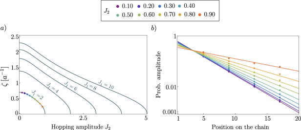
Figure 5: a) Localization length of edge states in a chain with first- and second-neighbour hoppings, given fixed $J^{\prime}_{1}$, as a function of $J_{2}$, in units of $J^{\prime}_{1}$, see equation (14). For each curve, $\zeta$ goes to zero when $J_{2}=J_{1}/2$, which corresponds to the overlapping of the bands. Colored dots in the $J_{1}=2$ curve correspond to the numerical data obtained by fitting the envelope of the edge states in a finite chain with $M=20$ to a exponential function of the form $\sim e^{-\lambda_{\mathrm{loc}}x}$, for different values of $J_{2}$ (see legend).
b) Probability amplitude of edge states wavefunction in logarithmic scale for $J_{1}=2J^{\prime}_{1}$, and $M=20$. Each color corresponds to the values of $J_{2}$ shown in the legend and in figure 5a. Plotmarkers represent the peak values of the edge states wavefunction, whereas continuous lines depict the numerical fitting to an exponential function. In logarithmic scale, they are represented as lines with slope $-\lambda_{\mathrm{loc}}$. As can be seen, the edge states do decay exponentially into the bulk when second-neighbour hoppings are added.

3.2 First- and third-neighbour hoppings

When first- and third-neighbour hoppings are considered, the system preserves time-reversal, particle-hole and chiral symmetry, and thus it belongs to the BDI class, just as the standard SSH model. Therefore, the topological invariant is well-defined and there is a one-to-one correspondence between its value and the number of edge states supported by the system.

The Bloch vector has the following non-zero components, $d_{x}(k)=J^{\prime}_{1}+(J_{1}+J^{\prime}_{3})\cos(k)+J_{3}\cos(2k)$, and $d_{y}(k)=(J_{1}-J^{\prime}_{3})\sin(k)+J_{3}\sin(2k)$, in terms of which the winding number can be calculated. A topological phase diagram is obtained as a function of $J^{\prime}_{3}$ and $J_{3}$ for different first-neighbour hoppings (see figure 6), setting to zero second-neighbour hoppings in order to preserve chiral symmetry. The presence of long-range hoppings enriches the phase map, making possible the existence of configurations with $\mathcal{W}=2$ and $\mathcal{W}=-1$.

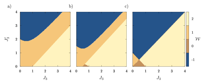
Figure 6: Topological phase diagram of as a function of third-neighbour hoppings, for different $J^{\prime}_{3}$, and $J_{3}$ (expressed in units of $J^{\prime}_{1}$). Second neighbours are set to zero in all of them $J_{2}=0$: a) $J_{1}=2J^{\prime}_{1}$, b) $J_{1}=1.5J^{\prime}_{1}$, c) $J_{1}=J^{\prime}_{1}$. Figures a) and b) fulfill $J^{\prime}_{1}/J_{1}<1$, which corresponds to a SSH topological insulator. Figure c) corresponds to an homogeneous chain ($J^{\prime}_{1}=J_{1}$) which is gapped due to third neighbour hoppings.

Interestingly, dimer chains with $\mathcal{W}=2$ support two pair of edge states. Owing to the presence of chiral symmetry, each pair carries two chiral partners, whose energies are related by $E_{\mathrm{e}}=-E_{\mathrm{o}}$. In the thermodynamic limit, when $M\rightarrow\infty$, these zero modes are located at either the right or left edge of the chain and can be chosen to have support on one of the sublattices, just as those in the SSH model. However, one remarkable distinction from the latter is the fact that each pair has a different spatial dependence, which in turn differ from that of the SSH model edge states. First, the peak of maximum probability amplitude is located at a different site for each pair. Depending on how hopping amplitudes are tuned, pairs can be maximally located at either the first, third, or fifth site of the chain. Moreover, the envelope of the edge states wavefunction decays exponentially into the bulk, but the probability amplitude on each site does not decrease monotonically. The larger the system, the more nicely the envelope fits into a exponential decay (see figure 7).

Figure 7: Absolute value of the edge states wavefunction of a chain with $M=40$ unit cells, and hopping amplitudes $J_{1}=4J^{\prime}_{1}/3$, $J_{2}=0$, $J^{\prime}_{3}=J^{\prime}_{1}/5$, and $J_{3}=J^{\prime}_{1}$ ($\mathcal{W}=2$). The continuous, blue line represents the fitting of the envelope to a exponential function. Each edge state depicted belongs to a different pair, and thus the peak of maximum probability occurs in a different site of the chain.

4 Periodic driving

As we have shown, phases with more than a single pair of edge states are possible, although they require unconventional hopping parameters, such that hopping amplitudes to further neighbours are larger than those to closer neighbours. In a regular system, however, one may expect hopping amplitudes to decrease with increasing distance. One way to overcome this consists in using a periodic driving, which in the high-frequency regime makes the system behave as if it were governed by an effective static Hamiltonian, with the possibility to change the effective hopping amplitudes by tuning the driving parameters [22].

With this purpose in mind, we include in the system Hamiltonian $H_{N}$ a time-dependent term $H_{AC}(t)=E(t)\sum_{j}x_{j}n_{j}$, corresponding to a homogeneous ac field $E(t)$ that couples to the charge (or mass) of the particles. $E(t)$ is a periodic function of time with period $T=2\pi/\omega$. Using a high-frequency expansion, we can derive an effective Hamiltonian $H_{\mathrm{eff}}$ expressed as a power series in $1/\omega$, see appendix B. To lowest order, $H_{\mathrm{eff}}$ is simply the time average of the total Hamiltonian over one period. Thus, the structure of the hoppings is maintained, but the hopping amplitudes become renormalized as

$$J_{ij}\rightarrow J_{ij}\frac{1}{T}\int_{0}^{T}dte^{iA(t)d_{ij}}\equiv J_{ij}f(E_{0}d_{ij}/\omega)\,.$$ (15)

Here $A(t)$ is the vector potential corresponding to the ac field $E(t)=-\partial_{t}A(t)$ and $d_{ij}=x_{i}-x_{j}$ is the distance between the $i^{th}$ and $j^{th}$ sites. We will assume that the decay of hopping amplitudes with distance is exponential, $J_{ij}=J_{0}e^{-d_{ij}/\lambda}$. Below, in table 1 we specify three different driving protocols studied in this work, with the corresponding hopping renormalization they produce.

Driving	Vector potential, $A$	Hopping renormalization, $f$
simple sinusoidal	$-\frac{E_{0}}{\omega}\sin(\omega t)$	$\mathcal{J}_{0}\left(\frac{E_{0}d_{ij}}{\omega}\right)$
double sinusoidal	$-\frac{E_{0}}{\omega}\left[\sin(\omega t)+\sin(3\omega t)\right]$	$\sum_{n}\mathcal{J}_{-3n}\left(\frac{E_{0}d_{ij}}{\omega}\right)\mathcal{J}_{n}\left(\frac{E_{0}d_{ij}}{\omega}\right)$
square-wave	$\left\{\begin{array}[]{l l l}-E_{0}t&\mathrm{if}&0<t<T/2\\ E_{0}(t-T)&\mathrm{if}&T/2<t<T\end{array}\right.$	$2i\left(e^{-iE_{0}Td_{ij}/2}-1\right)/E_{0}Td_{ij}$

Table 1: Different driving protocols with the corresponding hopping renormalization

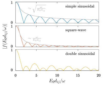
Figure 8: Comparison between the hopping renormalization functions of the different drivings studied. Note how the zeros of $f$ for the square-driving are equally spaced, while its envelope (grey line) decays faster than for the sinusoidal drivings.

For a simple sinusoidal drive with amplitude $E_{0}$ and frequency $\omega$, the hopping renormalization is given by the zeroth-order Bessel function of the first kind $\mathcal{J}_{0}(E_{0}d_{ij}/\omega)$ [23]. This allows to cancel the hoppings to next-nearest neighbours by tuning $E_{0}a/\omega$ to one of the zeros of $\mathcal{J}_{0}$. In this manner, it is possible to recover the chiral symmetry in chains with hoppings up to third neighbours. Nonetheless, it is impossible to zero out all even hoppings with this driving. Interestingly, we obtain winding numbers up to $\mathcal{W}=2$, but only for metallic phases, see figure 9.

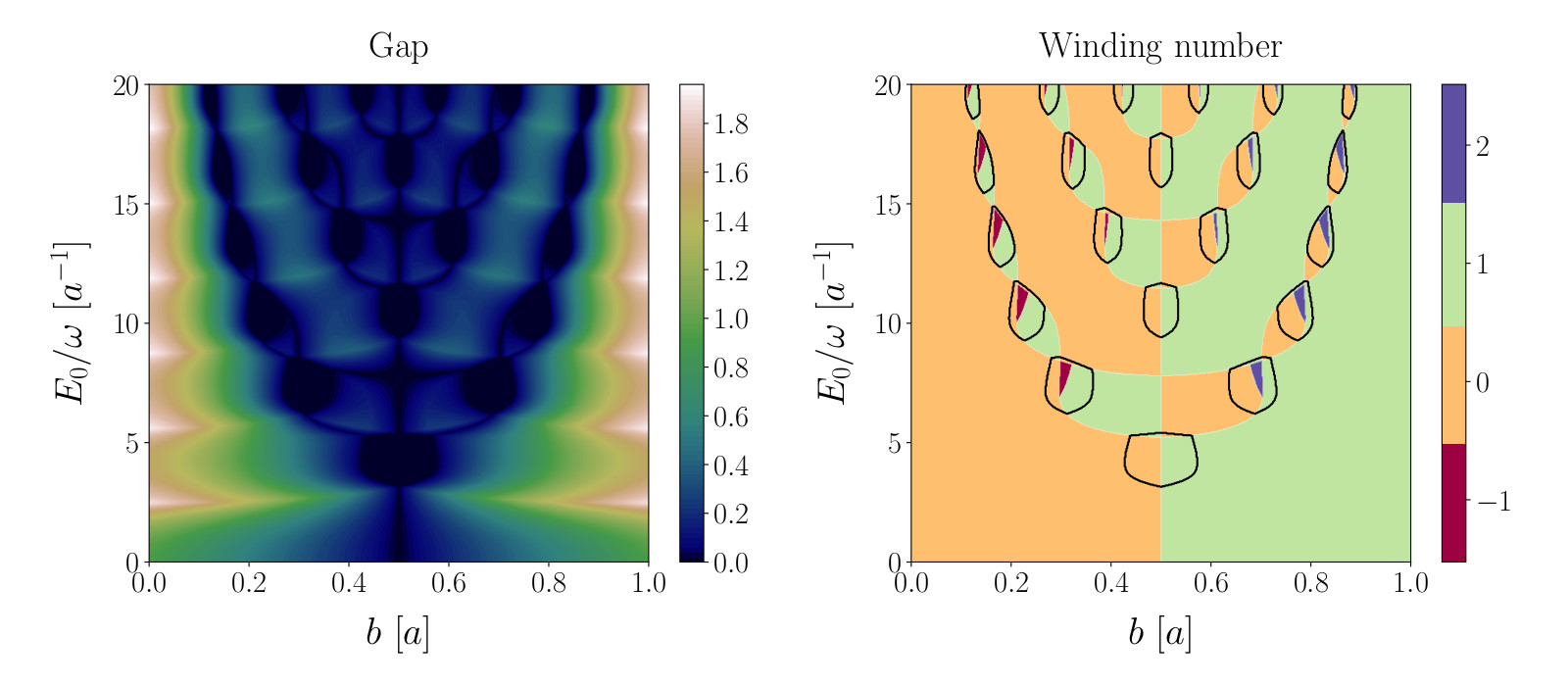
Figure 9: Phase diagram of the extended SSH model with a sinusoidal driving $A(t)=-\frac{E_{0}}{w}\sin(wt)$. Hopping amplitudes decay exponentially with distance. Chosing $\lambda=a$, only hoppings with range up to $N=10$ have a significant contribution. The gap is expressed in units of $J_{0}$. In the plot of the winding number, black curves show the contour level where the gap vanishes.

We can also consider more complicated drivings, such as a combination of two sinusoids with commensurate frequencies $E(t)=E_{0}\left[\cos(\omega t)+\cos(3\omega t)\right]$. As it can be seen in figure 10, with this driving we are able to produce gaped phases with winding numbers larger than 1, although the gap is smaller than in phases with smaller winding number.

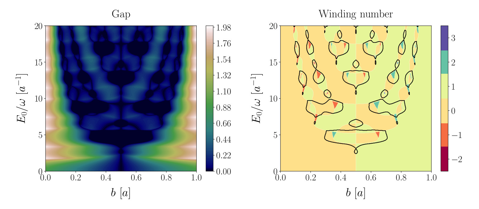
Figure 10: Phase diagram of the extended SSH model with a double sinusoidal driving $A(t)=-\frac{E_{0}}{w}[\sin(wt)+\sin(3w)]$. Hopping amplitudes decay exponentially with distance. Chosing $\lambda=a$, only hoppings with range up to $N=10$ have a significant contribution. The energy gap is expressed in units of $J_{0}$.

An appealing option is to use a square drive. As we show below, with this kind of driving it is possible to zero out all even hoppings simultaneously. Let us consider

$$E(t)=\left\{\begin{array}[]{l l l}E_{0}&\mathrm{if}&0<t<T/2\\ -E_{0}&\mathrm{if}&T/2<t<T\end{array}\right.\,,$$ (16)

which leads to a renormalization function $f$ whose zeros are evenly spaced on the possitive real axis, see figure 8 and table 1. Since the distances for all even hoppings are multiples of the lattice parameter $a$, it is now possible to cancel all of them by tuning $E_{0}/\omega=2a^{-1}$. In this way, we can enforce chiral symmetry on a system with arbitrarily long-range hopping terms. Despite this, with this kind of driving it is not possible to obtain winding numbers larger than 1 if the bare hopping amplitudes decay exponentially with distance.

5 Disorder

The effect of disorder in electronic systems has been an important subject since Anderson’s discussions on localisation [24]. Originally, he studied the propagation of a particle in a random potential, and showed that above certain critical values of disorder, localisation of the wavepackets happened. Strikingly, localisation was extremely dependent on the spatial dimension of the system, and in 1D, they were expected to localise for infinitesimal disorder [25]. Further studies have shown that there are exceptions to localisation in low dimensions, being the random dimer model one of the most well known cases, where inversion symmetry leads $\sqrt{N}$ states which are delocalised and contribute to the conductivity (i.e., they do not have zero measure in the thermodynamical limit [26]). More recent studies, including its effect on the topological phases [27, 28, 29], and on the role played by off-diagonal disorder [30, 31, 32] have also been done.
In this section we numerically study the effect of diagonal and off-diagonal uncorrelated disorder (in the onsite energies and hopping amplitudes, respectively) in the spectrum of both the standard and the extended SSH model. It must be stressed that this is different to the previously mentioned random dimer model, where disorder forms a random bipartite lattice with homogeneous hoppings.
First, we study diagonal disorder by considering the following Hamiltonian

$$H^{\prime}=H_{\mathrm{N}}+H_{\mathrm{diag}}=H_{\mathrm{N}}+\sum_{j=1}^{2M}\epsilon_{j}c^{\dagger}_{j}c_{j}\,,$$ (17)

where the second term shifts the onsite energies differently for each site by an amount $\epsilon_{j}$. We use random numbers following a Gaussian distribution centered at zero, so it is necessary to average the results over several repetitions. The figures included in this section have been obtained by taking the average over 100 repetitions. Diagonal disorder breaks sublattice symmetry and eliminates the zero-energy modes, therefore destroying the topological protection of the edge modes, both in the standard and the extended SSH model (see figure 11).

Figure 11: Effect of diagonal disorder on edge states in the extended SSH model with first- and third-neighbour hoppings, as a function of the diagonal disorder strength $\sigma$. Each pair of edge states has been depicted in a different color from the states in the bands (light purple). The dimer chain has $M=20$ unit cells and hopping amplitudes $J_{1}=1.2J^{\prime}_{1}$, $J_{2}=0$, $J^{\prime}_{3}=0.3J^{\prime}_{1}$, $J_{3}=0.9J^{\prime}_{1}$, which are chosen such that the system has $\mathcal{W}=2$ and preserves sublattice symmetry initially ($\sigma=0$). As can be seen, the absence of sublattice symmetry separates the edge states, destroying the topological phase and leading to the usual exponential localization for arbitrary disorder strength.

On the other hand, off-diagonal disorder refers to random hopping amplitudes,

$$H^{\prime\prime}=H_{\mathrm{N}}+H_{\mathrm{off-diag}}=H_{\mathrm{N}}+\sum_{|i-j|\leq N}\epsilon_{ij}c^{\dagger}_{i}c_{j}+\mathrm{H.c.}\,.$$ (18)

As it was shown in [32], systems with bipartite lattices display anomalous behaviour when off-diagonal disorder is considered. One reason for this is the presence of zero energy modes at the band centre. These states appear when sites in one sublattice couple only to sites of the other one, which is related to the differences observed in the previous section between the effect of adding even and odd neighbour hopping. Importantly, they showed that this type of disorder produces, at large distance and for states at $E=0$, slow decaying localisation of the form $\propto e^{-\lambda\sqrt{r}}$ (which produces a slower random walk behaviour than the usual exponential $e^{-\lambda r}$). Debate about whether these states are truly localised or not can be found in the literature [31].

Figure 12 shows how off-diagonal disorder affects edge states in both the standard and extended SSH model for a configuration with $\mathcal{W}=2$ and first- to third- neighbour hoppings. As expected, the pair of zero-energy modes in a SSH chain is robust under this type of perturbation, until disorder is of the order of the gap $\sigma\propto\Delta$. Then, the intra- and inter-dimer hopping cannot be differentiated, the bands mix and eventually the edge modes separate. However, it is interesting to see how each pair of edge states behaves differently when disorder is increased in the extended-SSH configuration under consideration.

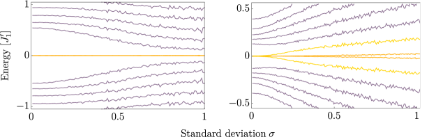
Figure 12: Effect of off-diagonal disorder on edge states in the standard and extended SSH model with first- and third-neighbour hoppings. Each pair of edge states has been depicted in a different color from the states in the bands (light purple).
(a) SSH model: finite chain with $M=20$ and $J_{1}=1.5J^{\prime}_{1}$ , as a function of the off-diagonal disorder strength $\sigma$.
(b) Extended SSH model: finite chain with $M=20$ and hoppings: $J_{1}=1.5J^{\prime}_{1}$, $J_{2}=0$, $J^{\prime}_{3}=0.3J^{\prime}_{1}$, $J_{3}=0.9J^{\prime}_{1}$, as a function of the off-diagonal disorder strength $\sigma$. Hoppings are chosen such that the system has ($\mathcal{W}=2$) initially.

6 Conclusions

In this work, we have studied a generalized model for a dimer chain including long-range hoppings, which naturally occur in physical systems. Although seemingly equal, the effect of hopping processes connecting the same sublattice (even hoppings), and processes connecting different sublattices (odd hoppings) is very different. The former breaks particle-hole symmetry, and changes the topological class from BDI to AI. Nevertheless, the presence of space inversion symmetry forces the topological invariant to have quantized values, and the appearance of edge states protected only by this symmetry. As a consequence, the number of edge states now changes independently of the topological invariant, as they can enter the bulk bands if the hopping amplitudes connecting different sublattices is large enough. On the contrary, hopping between different sublattices preserves the fundamental symmetries, and allows for phases with larger values of the topological invariant and larger numbers of edge-state pairs.

We propose the use of an ac driving to tune the topological properties of the system. Three different drivings are analyzed. Interestingly, we show that with a square-wave driving it is possible to cancel all even hoppings simultaneously, restoring the symmetries of the standard SSH model.

Finally, we have investigated the effect of disorder. In the case of a chain with only odd hoppings, the edge states are robust against off-diagonal disorder, while they loose their protection as long as we introduce even hoppings. We also show that in phases with more than a single pair of edge states, their energies departure from zero at different rates as the strength of diagonal disorder is increased.

Appendix A Topological invariant in 1D systems

For 1D systems, we can define a topological invariant through the Zak phase [33], which is the integration of the Berry connection over the first Brillouin zone (FBZ).

$$\mathcal{Z}_{n}=i\int_{\mathrm{FBZ}}dk\mathcal{h}u_{n}(k)|\partial_{k}u_{n}(k)\mathcal{i}\,,$$ (19)

where $n$ is the band subscript ($n=\pm$) and $|u_{n}(k)\mathcal{i}$ are the Bloch functions. The Zak phase is a particular case of the Berry phase [34], which is the geometric phase acquired by an eigenstate of the system when it is made to evolve cyclically in the parameter space of the problem under consideration. When this concept is applied to the dynamics of electrons in periodic solids, the Berry phase is refered to as the Zak phase and the parameter space, the Brillouin zone, is naturally furnished by the system itself. When $k$ is sweeped across the FBZ $k=0\rightarrow 2\pi$, eigenstates evolves through a closed path, picking up a phase given by (19).
The Zak phase is closely related to the bulk electric polarization, as has been shown in the so-called modern theory of polarization . The bulk electric polarization is given by $P_{\mathrm{bulk}}=\mathcal{Z}/2\pi$. In a neutral chain, $P_{\mathrm{total}}=P_{\mathrm{edge}}+P_{\mathrm{bulk}}=0$. If the bulk polarization is non-zero, there must be accumulation of charge at the edges, thus explaining the relation between a non-zero value of the Zak phase and the presence of edge states.
On the other hand, Bloch functions are eigenstates of the bulk momentum-space Hamiltonian, $\mathcal{H}|u_{n}(k)\mathcal{i}=E_{n}(k)|u_{n}(k)\mathcal{i}$. The Zak phase can be understood as the rotation angle $|u_{n}(k)\mathcal{i}$ undergoes when it is parallel transported along the FBZ. The curvature of the FBZ, reflected in the Berry connection, is responsible for the phase that the Bloch function picks up.

Equivalently, it can be expressed in terms of the winding of the closed curve defined by the Bloch vector as $k=0\rightarrow 2\pi$ around the origin,

$$\mathcal{W}=\frac{\mathcal{Z}}{\pi}=\frac{1}{2\pi}\int_{\mathrm{FBZ}}\frac{d_{x}\partial_{k}d_{y}-d_{y}\partial_{k}d_{x}}{d_{x}^{2}+d_{y}^{2}}dk\,.$$ (20)

In the SSH model, the curve $\gamma=(d_{x}(k),d_{y}(k))=(J^{\prime}_{1}+J_{1}\cos(k),J_{1}\sin(k))$ describes a circunference centered at $(J^{\prime}_{1},0)$ and radius $J_{1}$. Thus, the topology of a system is determined by whether or not the previous curve encloses the origin. In this geometric picture, we can identify topologically equivalent configurations as those whose $\gamma$ can be continuously transformed into one another without passing through the origin. In the extended SSH model, the topological phase diagram is enriched and $\gamma$ displays more complex geometries, giving raise to larger values of the winding.

Appendix B Floquet theory

The starting Hamiltonian is $H(t)=H_{N}+H_{AC}(t)$. For a time-periodic Hamiltonian, $H(t+T)=H(t)$ with $T=2\pi/\omega$, Floquet’s theorem permits us to write the time-evolution operator $U(t_{2},t_{1})$ as

$$U(t_{2},t_{1})=e^{-iK(t_{2})}e^{-iH_{\mathrm{eff}}(t_{2}-t_{1})}e^{iK(t_{1})}\,,$$ (21)

where $H_{\mathrm{eff}}$ is a time independent (effective) Hamiltonian and $K(t)$ is a $T$-periodic Hermitian operator. $H_{\mathrm{eff}}$ governs the long-term dynamics whereas $e^{-iK(t)}$, also known as the micromotion operator, accounts for the fast dynamics occurring within a period. Following several perturbative methods [35, 36], it is possible to find expressions for these operators as power series in $1/\omega$

$$H_{\mathrm{eff}}=\sum\limits_{n=0}^{\infty}\frac{H^{[n]}}{\omega^{n}}\,,\quad K(t)=\sum\limits_{n=0}^{\infty}\frac{K^{[n]}(t)}{\omega^{n}}\,.$$ (22)

The different terms in these expansions have a progressively more complicated dependence on the Fourier components of the original Hamiltonian, ${H^{(q)}=T^{-1}\int_{0}^{T}H(t)e^{i\omega qt}dt}$. The first three of them are:

$$H^{[0]}=H^{(0)}\,,\quad H^{[1]}=\sum\limits_{q\neq 0}\frac{H^{(-q)}H^{(q)}}{q}\,,$$ (23)

$$H^{[2]}=\sum\limits_{q,p\neq 0}\left(\frac{H^{(-q)}H^{(q-p)}H^{(p)}}{qp}-\frac{H^{(-q)}H^{(q)}H^{(0)}}{q^{2}}\right)\,.$$ (24)

Before deriving the effective Hamiltonian, in order to obtain a result that is non-perturbative in the ac field amplitude, it is convenient to transform the original Hamiltonian into the rotating frame with respect to the ac field

$$\tilde{H}(t)=\mathcal{U}^{\dagger}(t)H(t)\mathcal{U}(t)-i\mathcal{U}^{\dagger}(t)\partial_{t}\mathcal{U}(t)\,,$$ (25)

$$\mathcal{U}(t)=e^{-i\int H_{AC}(t)dt}\,.$$ (26)

This leads to

$$\tilde{H}(t)=\sum_{i,j}J_{ij}e^{iA(t)d_{ij}}c^{\dagger}_{i}c_{j}\,.$$ (27)

References

References

- [1] Thouless D J, Kohmoto M, Nightingale M P and den Nijs M 1982 Phys. Rev. Lett. 49(6) 405–408 URL https://link.aps.org/doi/10.1103/PhysRevLett.49.405
- [2] Laughlin R B 1983 Phys. Rev. Lett. 50(18) 1395–1398 URL https://link.aps.org/doi/10.1103/PhysRevLett.50.1395
- [3] König M, Wiedmann S, Brüne C, Roth A, Buhmann H, Molenkamp L W, Qi X L and Zhang S C 2007 318 766–770
- [4] Cinchetti M 2014 Nature Nanotechnology 9 965 URL http://dx.doi.org/10.1038/nnano.2014.284
- [5] Nagaosa T 2013 Nature Nanotechnology 8 899–911 URL http://dx.doi.org/10.1038/nnano.2013.243
- [6] Kitaev A 2003 Annals of Physics 303 2 – 30 ISSN 0003-4916 URL http://www.sciencedirect.com/science/article/pii/S0003491602000180
- [7] Plugge S, Rasmussen A, Egger R and Flensberg K 2017 New Journal of Physics 19 012001 URL http://stacks.iop.org/1367-2630/19/i=1/a=012001
- [8] Li L, Yang C and Chen S 2015 EPL (Europhysics Letters) 112 10004 URL http://stacks.iop.org/0295-5075/112/i=1/a=10004
- [9] Li L, Xu Z and Chen S 2014 Phys. Rev. B 89(8) 085111 URL https://link.aps.org/doi/10.1103/PhysRevB.89.085111
- [10] Su W P, Schrieffer J R and Heeger A J 1980 Phys. Rev. B 22(4) 2099–2111 URL https://link.aps.org/doi/10.1103/PhysRevB.22.2099
- [11] Takayama H, Lin-Liu Y R and Maki K 1980 Phys. Rev. B 21(6) 2388–2393 URL https://link.aps.org/doi/10.1103/PhysRevB.21.2388
- [12] Kivelson S and Heim D E 1982 Phys. Rev. B 26(8) 4278–4292 URL https://link.aps.org/doi/10.1103/PhysRevB.26.4278
- [13] Marcos Atala Monika Aidelsburger J T B D A T K E D and Bloch I 2013 Nature Physics 9 795–800
- [14] Rice M J and Mele E J 1982 Phys. Rev. Lett. 49(19) 1455–1459 URL https://link.aps.org/doi/10.1103/PhysRevLett.49.1455
- [15] Longhi S 2013 Opt. Lett. 38 3716–3719 URL http://ol.osa.org/abstract.cfm?URI=ol-38-19-3716
- [16] Wei Tan Yong Sun H C S Q S 2014 Scientific Reports 4 3842
- [17] Meng Xiao Guancong Ma Z Y P S Z Q Z C T C 2014 Nature Physics 11 240–244
- [18] Zhaoju Yang F G B Z 2016 Scientific Reports 6 29202
- [19] Ryu S, Schnyder A P, Furusaki A and Ludwig A W W 2010 New Journal of Physics 12 065010 URL http://stacks.iop.org/1367-2630/12/i=6/a=065010
- [20] Asbóth J, Oroszlány L and Pályi A 2016 A Short Course on Topological Insulators: Band Structure and Edge States in One and Two Dimensions Lecture Notes in Physics (Springer International Publishing) ISBN 9783319256078 URL https://books.google.es/books?id=RWKhCwAAQBAJ
- [21] Delplace P, Ullmo D and Montambaux G 2011 Phys. Rev. B 84(19) 195452 URL https://link.aps.org/doi/10.1103/PhysRevB.84.195452
- [22] Gómez-León A and Platero G 2013 Phys. Rev. Lett. 110(20) 200403 URL https://link.aps.org/doi/10.1103/PhysRevLett.110.200403
- [23] Grifoni M and Hänggi P 1998 Physics Reports 304 229 – 354 ISSN 0370-1573 URL http://www.sciencedirect.com/science/article/pii/S0370157398000222
- [24] Anderson P W 1958 Phys. Rev. 109(5) 1492–1505 URL https://link.aps.org/doi/10.1103/PhysRev.109.1492
- [25] Abrahams E, Anderson P W, Licciardello D C and Ramakrishnan T V 1979 Phys. Rev. Lett. 42(10) 673–676 URL https://link.aps.org/doi/10.1103/PhysRevLett.42.673
- [26] Dunlap D H, Wu H L and Phillips P W 1990 Phys. Rev. Lett. 65(1) 88–91 URL https://link.aps.org/doi/10.1103/PhysRevLett.65.88
- [27] Bardarson J H, Brouwer P W and Moore J E 2010 Phys. Rev. Lett. 105(15) 156803 URL https://link.aps.org/doi/10.1103/PhysRevLett.105.156803
- [28] Zhang X, Guo H and Feng S 2012 Journal of Physics: Conference Series 400 042078 URL http://stacks.iop.org/1742-6596/400/i=4/a=042078
- [29] Li J, Chu R L, Jain J K and Shen S Q 2009 Phys. Rev. Lett. 102(13) 136806 URL https://link.aps.org/doi/10.1103/PhysRevLett.102.136806
- [30] Pendry J B 1982 Journal of Physics C: Solid State Physics 15 5773 URL http://stacks.iop.org/0022-3719/15/i=28/a=009
- [31] Biswas P, Cain P, Römer R and Schreiber M 2000 physica status solidi (b) 218 205–209 ISSN 1521-3951 URL http://dx.doi.org/10.1002/(SICI)1521-3951(200003)218:1<205::AID-PSSB205>3.0.CO;2-B
- [32] Inui M, Trugman S A and Abrahams E 1994 Phys. Rev. B 49(5) 3190–3196 URL https://link.aps.org/doi/10.1103/PhysRevB.49.3190
- [33] Zak J 1989 Phys. Rev. Lett. 62(23) 2747–2750 URL https://link.aps.org/doi/10.1103/PhysRevLett.62.2747
- [34] V Berry M 1984 392 45–57
- [35] Eckardt A and Anisimovas E 2015 New J. of Phys. 17 093039 URL http://stacks.iop.org/1367-2630/17/i=9/a=093039
- [36] Bukov M, D’Alessio L and Polkovnikov A 2015 Adv. in Phys., vol. 64, No. 2 139–226