Quasi-Optimal Partial Order Reduction

Abstract

A dynamic partial order reduction (DPOR) algorithm is optimal when it always explores at most one representative per Mazurkiewicz trace. Existing literature suggests that the reduction obtained by the non-optimal, state-of-the-art Source-DPOR (SDPOR) algorithm is comparable to optimal DPOR. We show the first program with $\mathop{\mathcal{O}}(n)$ Mazurkiewicz traces where SDPOR explores $\mathop{\mathcal{O}}(2^{n})$ redundant schedules. We furthermore identify the cause of this blow-up as an NP-hard problem. Our main contribution is a new approach, called Quasi-Optimal POR, that can arbitrarily approximate an optimal exploration using a provided constant $k$. We present an implementation of our method in a new tool called Dpu using specialised data structures. Experiments with Dpu, including Debian packages, show that optimality is achieved with low values of $k$, outperforming state-of-the-art tools.

1 Introduction

Dynamic partial-order reduction (DPOR) [10, 1, 19] is a mature approach to mitigate the state explosion problem in stateless model checking of multithreaded programs. DPORs are based on Mazurkiewicz trace theory [13], a true-concurrency semantics where the set of executions of the program is partitioned into equivalence classes known as Mazurkiewicz traces (M-traces). In a DPOR, this partitioning is defined by an independence relation over concurrent actions that is computed dynamically and the method explores executions which are representatives of M-traces. The exploration is sound when it explores all M-traces, and it is considered optimal [1] when it explores each M-trace only once.

Since two independent actions might have to be explored from the same state in order to explore all M-traces, a DPOR algorithm uses independence to compute a provably-sufficient subset of the enabled transitions to explore for each state encountered. Typically this involves the combination of forward reasoning (persistent sets [11] or source sets [1, 4]) with backward reasoning (sleep sets [11]) to obtain a more efficient exploration. However, in order to obtain optimality, a DPOR is forced to compute sequences of transitions (as opposed to sets of enabled transitions) that avoid visiting a previously visited M-trace. These sequences are stored in a data structure called wakeup trees in [1] and known as alternatives in [19]. Computing these sequences thus amounts to deciding whether the DPOR needs to visit yet another M-trace (or all have already been seen).

In this paper, we prove that computing alternatives in an optimal DPOR is an NP-complete problem. To the best our knowledge this is the first formal complexity result on this important subproblem that optimal and non-optimal DPORs need to solve. The program shown in Fig. 1 (a) illustrates a practical consequence of this result: the non-optimal, state-of-the-art SDPOR algorithm [1] can explore here $\mathop{\mathcal{O}}(2^{n})$ interleavings but the program has only $\mathop{\mathcal{O}}(n)$ M-traces.

(a)  $w_{0}$ $w_{1}$ $w_{2}$ count master $x_{0}=7$ $x_{1}=8$ $x_{2}=9$ $c=1$ $i=c$ $c=2$ $x_{i}=0$

Figure 1: (a): Programs; (b): Partially-ordered executions;

The program contains $n\mathrel{:=}3$ writer threads $w_{0},w_{1},w_{2}$, each writing to a different variable. The thread count increments $n-1$ times a zero-initialized counter $c$. Thread master reads $c$ into variable $i$ and writes to $x_{i}$.

The statements $x_{0}=7$ and $x_{1}=8$ are independent because they produce the same state regardless of their execution order. Statements $i=c$ and any statement in the count thread are dependent or interfering: their execution orders result in different states. Similarly, $x_{i}=0$ interferes with exactly one writer thread, depending on the value of $i$.

Using this independence relation, the set of executions of this program can be partitioned into six M-traces, corresponding to the six partial orders shown in Fig. 1 (b). Thus, an optimal DPOR explores six executions ($2n$-executions for $n$ writers). We now show why SDPOR explores $\mathop{\mathcal{O}}(2^{n})$ in the general case. Conceptually, SDPOR is a loop that (1) runs the program, (2) identifies two dependent statements that can be swapped, and (3) reverses them and re-executes the program. It terminates when no more dependent statements can be swapped.

Consider the interference on the counter variable $c$ between the master and the count thread. Their execution order determines which writer thread interferes with the master statement $x_{i}=0$. If $c=1$ is executed just before $i=c$, then $x_{i}=0$ interferes with $w_{1}$. However, if $i=c$ is executed before, then $x_{i}=0$ interferes with $w_{0}$. Since SDPOR does not track relations between dependent statements, it will naively try to reverse the race between $x_{i}=0$ and all writer threads, which results in exploring $\mathop{\mathcal{O}}(2^{n})$ executions. In this program, exploring only six traces requires understanding the entanglement between both interferences as the order in which the first is reversed determines the second.

As a trade-off solution between solving this NP-complete problem and potentially explore an exponential number of redundant schedules, we propose a hybrid approach called Quasi-Optimal POR (QPOR) which can turn a non-optimal DPOR into an optimal one. In particular, we provide a polynomial algorithm to compute alternative executions that can arbitrarily approximate the optimal solution based on a user specified constant $k$. The key concept is a new notion of $k$-partial alternative, which can intuitively be seen as a “good enough” alternative: they revert two interfering statements while remembering the resolution of the last $k-1$ interferences.

The major differences between QPOR and the DPORs of [1] are that: 1) QPOR is based on prime event structures [17], a partial-order semantics that has been recently applied to programs [19, 21], instead of a sequential view to thread interleaving, and 2) it computes $k$-partial alternatives with an $\mathop{\mathcal{O}}(n^{k})$ algorithm while optimal DPOR corresponds to computing $\infty$-partial alternatives with an $\mathop{\mathcal{O}}(2^{n})$ algorithm. For the program shown in Fig. 1 (a), QPOR achieves optimality with $k=2$ because races are coupled with (at most) another race. As expected, the cost of computing $k$-partial alternatives and the reductions obtained by the method increase with higher values of $k$.

Finding $k$-partial alternatives requires decision procedures for traversing the causality and conflict relations in event structures. Our main algorithmic contribution is to represent these relations as a set of trees where events are encoded as one or two nodes in two different trees. We show that checking causality/conflict between events amounts to an efficient traversal in one of these trees.

In summary, our main contributions are:

• Proof that computing alternatives for optimal DPOR is NP-complete (Sec. 4).

• Efficient data structures and algorithms for (1) computing $k$-partial alternatives in polynomial time, and (2) represent and traverse partial orders (Sec. 5).

• Implementation of QPOR in a new tool called Dpu and experimental evaluations against SDPOR in Nidhugg and the testing tool Maple (Sec. 6).

• Benchmarks with $\mathop{\mathcal{O}}(n)$ M-traces where SDPOR explores $\mathop{\mathcal{O}}(2^{n})$ executions (Sec. 6).

Furthermore, in Sec. 6 we show that: (1) low values of $k$ often achieve optimality; (2) even with non-optimal explorations Dpu greatly outperforms Nidhugg; (3) Dpu copes with production code in Debian packages and achieves much higher state space coverage and efficiency than Maple.

Proofs for all our formal results are available in the appendix of this manuscript.

2 Preliminaries

In this section we provide the formal background used throughout the paper.

Concurrent Programs.

We consider deterministic concurrent programs composed of a fixed number of threads that communicate via shared memory and synchronize using mutexes (Fig. 1 (a) can be trivially modified to satisfy this). We also assume that local statements can only modify shared memory within a mutex block. Therefore, it suffices to only consider races of mutex accesses.

Formally, a concurrent program is a structure $P\mathrel{:=}\langle\mathcal{M},\mathcal{L},T,m_{0},l_{0}\rangle$, where $\mathcal{M}$ is the set of memory states (valuations of program variables, including instruction pointers), $\mathcal{L}$ is the set of mutexes, $m_{0}$ is the initial memory state, $l_{0}$ is the initial mutexes state and $T$ is the set of thread statements. A thread statement $t\mathrel{:=}\langle i,f\rangle$ is a pair where $i\in\mathbb{N}$ is the thread identifier associated with the statement and $f\colon\mathcal{M}\to(\mathcal{M}\times\Lambda)$ is a partial function that models the transformation of the memory as well as the effect $\Lambda\mathrel{:=}{\{\texttt{loc}\mathclose{\}}}\cup({\{\texttt{acq},\texttt{rel}\mathclose{\}}}\times\mathcal{L})$ of the statement with respect to thread synchronization. Statements of loc effect model local thread code. Statements associated with $\langle\texttt{acq},x\rangle$ or $\langle\texttt{rel},x\rangle$ model lock and unlock operations on a mutex $x$. Finally, we assume that (1) functions $f$ are PTIME-decidable; (2) acq/rel statements do not modify the memory; and (3) loc statements modify thread-shared memory only within lock/unlock blocks. When (3) is violated, then $P$ has a datarace (undefined behavior in almost all languages), and our technique can be used to find such statements, see Sec. 6.

We use labelled transition systems ($LTS$) semantics for our programs. We associate a program $P$ with the $LTS$ $M_{P}\mathrel{:=}\langle\mathcal{S},{\to},A,s_{0}\rangle$. The set $\mathcal{S}\mathrel{:=}\mathcal{M}\times(\mathcal{L}\to{\{0,1\mathclose{\}}})$ are the states of $M_{P}$, i.e., pairs of the form $\langle m,v\rangle$ where $m$ is the state of the memory and $v$ indicates when a mutex is locked (1) or unlocked (0). The actions in $A\subseteq\mathbb{N}\times\Lambda$ are pairs $\langle i,b\rangle$ where $i$ is the identifier of the thread that executes some statement and $b$ is the effect of the statement. We use the function $p\colon A\to\mathbb{N}$ to retrieve the thread identifier. The transition relation ${\to}\subseteq\mathcal{S}\times A\times\mathcal{S}$ contains a triple $\langle m,v\rangle\mathrel{\raisebox{-1.9pt}{$\xrightarrow{\langle i,b\rangle}$}}\langle m^{\prime},v^{\prime}\rangle$ exactly when there is some thread statement $\langle i,f\rangle\in T$ such that $f(m)=\langle m^{\prime},b\rangle$ and either (1) $b=\texttt{loc}$ and $v^{\prime}=v$, or (2) $b=\langle\texttt{acq},x\rangle$ and $v(x)=0$ and $v^{\prime}=v_{|x\mapsto 1}$, or (3) $b=\langle\texttt{rel},x\rangle$ and $v^{\prime}=v_{|x\mapsto 0}$. Notation $f_{x\mapsto y}$ denotes a function that behaves like $f$ for all inputs except for $x$, where $f(x)=y$. The initial state is $s_{0}\mathrel{:=}\langle m_{0},l_{0}\rangle$.

Furthermore, if $s\mathrel{\raisebox{-1.9pt}{$\xrightarrow{a}$}}s^{\prime}$ is a transition, the action $a$ is enabled at $s$. Let $\mathop{\mathit{enabl}}(s)$ denote the set of actions enabled at $s$. A sequence $\sigma\mathrel{:=}a_{1}\ldots a_{n}\in A^{*}$ is a run when there are states $s_{1},\ldots,s_{n}$ satisfying $s_{0}\mathrel{\raisebox{-1.9pt}{$\xrightarrow{a_{1}}$}}s_{1}\ldots\mathrel{\raisebox{-1.9pt}{$\xrightarrow{a_{n}}$}}s_{n}$. We define $\mathop{\mathit{state}}(\sigma)\mathrel{:=}s_{n}$. We let $\mathop{\mathit{runs}}(M_{P})$ denote the set of all runs and $\mathop{\mathit{reach}}(M_{P})\mathrel{:=}{\{\mathop{\mathit{state}}(\sigma)\in\mathcal{S}\colon\sigma\in\mathop{\mathit{runs}}(M_{P})\mathclose{\}}}$ the set of all reachable states.

Independence.

Dynamic partial-order reduction methods use a notion called independence to avoid exploring concurrent interleavings that lead to the same state. We recall the standard notion of independence for actions in [11]. Two actions $a,a^{\prime}\in A$ commute at a state $s\in\mathcal{S}$ iff

• if $a\in\mathop{\mathit{enabl}}(s)$ and $s\mathrel{\raisebox{-1.9pt}{$\xrightarrow{a}$}}s^{\prime}$, then $a^{\prime}\in\mathop{\mathit{enabl}}(s)$ iff $a^{\prime}\in\mathop{\mathit{enabl}}(s^{\prime})$; and

• if $a,a^{\prime}\in\mathop{\mathit{enabl}}(s)$, then there is a state $s^{\prime}$ such that $s\mathrel{\raisebox{-1.9pt}{$\xrightarrow{a.a^{\prime}}$}}s^{\prime}$ and $s\mathrel{\raisebox{-1.9pt}{$\xrightarrow{a^{\prime}.a}$}}s^{\prime}$.

Independence between actions is an under-approximation of commutativity. A binary relation ${\mathrel{\diamondsuit}}\subseteq A\times A$ is an independence on $M_{P}$ if it is symmetric, irreflexive, and every pair $\langle a,a^{\prime}\rangle$ in $\mathrel{\diamondsuit}$ commutes at every state in $\mathop{\mathit{reach}}(M_{P})$.

In general $M_{P}$ has multiple independence relations, clearly $\emptyset$ is always one of them. We define relation ${\mathrel{\diamondsuit}_{P}}\subseteq A\times A$ as the smallest irreflexive, symmetric relation where $\langle i,b\rangle\mathrel{\diamondsuit}_{P}\langle i^{\prime},b^{\prime}\rangle$ holds if $i\neq i^{\prime}$ and either $b=\texttt{loc}$ or $b=\texttt{acq}\ x$ and $b^{\prime}\not\in{\{\texttt{acq}\ x,\texttt{rel}\ x\mathclose{\}}}$. By construction $\mathrel{\diamondsuit}_{P}$ is always an independence.

Labelled Prime Event Structures.

Prime event structures (pes) are well-known non-interleaving, partial-order semantics [16, 8, 7]. Let $X$ be a set of actions. A pes over $X$ is a structure $\mathcal{E}\mathrel{:=}\langle E,<,\mathrel{\#},h\rangle$ where $E$ is a set of events, ${<}\subseteq E\times E$ is a strict partial order called causality relation, ${\mathrel{\#}}\subseteq E\times E$ is a symmetric, irreflexive conflict relation, and $h\colon E\to X$ is a labelling function. Causality represents the happens-before relation between events, and conflict between two events expresses that any execution includes at most one of them. Fig. 2 (b) shows a pes over $\mathbb{N}\times\Lambda$ where causality is depicted by arrows, conflicts by dotted lines, and the labelling $h$ is shown next to the events, e.g., $1<5$, $8<12$, $2\mathrel{\#}8$, and $h(1)=\langle 0,\texttt{loc}\rangle$. The history of an event $e$, $\left\lceil e\right\rceil\mathrel{:=}{\{e^{\prime}\in E\colon e^{\prime}<e\mathclose{\}}}$, is the least set of events that need to happen before $e$.

The notion of concurrent execution in a pes is captured by the concept of configuration. A configuration is a (partially ordered) execution of the system, i.e., a set $C\subseteq E$ of events that is causally closed (if $e\in C$, then $\left\lceil e\right\rceil\subseteq C$) and conflict-free (if $e,e^{\prime}\in C$, then $\lnot(e\mathrel{\#}e^{\prime})$). In Fig. 2 (b), the set ${\{8,9,15\mathclose{\}}}$ is a configuration, but ${\{3\mathclose{\}}}$ or ${\{1,2,8\mathclose{\}}}$ are not. We let $\mathop{\mathit{conf}}(\mathcal{E})$ denote the set of all configurations of $\mathcal{E}$, and $[e]\mathrel{:=}\left\lceil e\right\rceil\cup{\{e\mathclose{\}}}$ the local configuration of $e$. In Fig. 2 (b), $[11]={\{1,8,9,10,11\mathclose{\}}}$. A configuration represents a set of interleavings over $X$. An interleaving is a sequence in $X^{*}$ that labels any topological sorting of the events in $C$. We denote by $\mathop{\mathit{inter}}(C)$ the set of interleavings of $C$. In Fig. 2 (b), $\mathop{\mathit{inter}}({\{1,8\mathclose{\}}})={\{ab,ba\mathclose{\}}}$ with $a\mathrel{:=}\langle 0,\texttt{loc}\rangle$ and $b\mathrel{:=}\langle 1,\texttt{acq}\ m\rangle$.

The extensions of $C$ are the events not in $C$ whose histories are included in $C$: $\mathop{\mathit{ex}}(C)\mathrel{:=}{\{e\in E\colon e\notin C\land\left\lceil e\right\rceil\subseteq C\mathclose{\}}}$. The enabled events of $C$ are the extensions that can form a larger configuration: $\mathop{\mathit{en}}(C)\mathrel{:=}{\{e\in\mathop{\mathit{ex}}(C)\colon C\cup{\{e\mathclose{\}}}\in\mathop{\mathit{conf}}(\mathcal{E})\mathclose{\}}}$. Finally, the conflicting extensions of $C$ are the extensions that are not enabled: $\mathop{\mathit{cex}}(C)\mathrel{:=}\mathop{\mathit{ex}}(C)\setminus\mathop{\mathit{en}}(C)$. In Fig. 2 (b), $\mathop{\mathit{ex}}({\{1,8\mathclose{\}}})={\{2,9,15\mathclose{\}}}$, $\mathop{\mathit{en}}({\{1,8\mathclose{\}}})={\{9,15\mathclose{\}}}$, and $\mathop{\mathit{cex}}({\{1,8\mathclose{\}}})={\{2\mathclose{\}}}$. See [20] for more information on pes concepts.

Parametric Unfolding Semantics.

We recall the program pes semantics of [19, 20] (modulo notation differences). For a program $P$ and any independence $\mathrel{\diamondsuit}$ on $M_{P}$ we define a pes $\mathcal{U}_{P,\mathrel{\diamondsuit}}$ that represents the behavior of $P$, i.e., such that the interleavings of its set of configurations equals $\mathop{\mathit{runs}}(M_{P})$.

Each event in $\mathcal{U}_{P,\mathrel{\diamondsuit}}$ is defined by a canonical name of the form $e\mathrel{:=}\langle a,H\rangle$, where $a\in A$ is an action of $M_{P}$ and $H$ is a configuration of $\mathcal{U}_{P,\mathrel{\diamondsuit}}$. Intuitively, $e$ represents the action $a$ after the history (or the causes) $H$. Fig. 2 (b) shows an example. Event 11 is $\langle\langle 0,\texttt{acq}\ m\rangle,{\{1,8,9,10\mathclose{\}}}\rangle$ and event 1 is $\langle\langle 0,\texttt{loc}\rangle,\emptyset\rangle$. Note the inductive nature of the name, and how it allows to uniquely identify each event. We define the state of a configuration as the state reached by any of its interleavings. Formally, for $C\in\mathop{\mathit{conf}}(\mathcal{U}_{P,\mathrel{\diamondsuit}})$ we define $\mathop{\mathit{state}}(C)$ as $s_{0}$ if $C=\emptyset$ and as $\mathop{\mathit{state}}(\sigma)$ for some $\sigma\in\mathop{\mathit{inter}}(C)$ if $C\neq\emptyset$. Despite its appearance $\mathop{\mathit{state}}(C)$ is well-defined because all sequences in $\mathop{\mathit{inter}}(C)$ reach the same state, see [20] for a proof.

Definition 1 (Unfolding)

Given a program $P$ and some independence relation $\mathrel{\diamondsuit}$ on $M_{P}\mathrel{:=}\langle\mathcal{S},\to,A,s_{0}\rangle$, the unfolding of $P$ under $\mathrel{\diamondsuit}$, denoted $\mathcal{U}_{P,\mathrel{\diamondsuit}}$, is the pes over $A$ constructed by the following fixpoint rules:

1. Start with a pes $\mathcal{E}\mathrel{:=}\langle E,<,{\mathrel{\#}},h\rangle$ equal to $\langle\emptyset,\emptyset,\emptyset,\emptyset\rangle$.

2. Add a new event $e\mathrel{:=}\langle a,C\rangle$ to $E$ for any configuration $C\in\mathop{\mathit{conf}}(\mathcal{E})$ and any action $a\in A$ if $a$ is enabled at $\mathop{\mathit{state}}(C)$ and $\lnot(a\mathrel{\diamondsuit}h(e^{\prime}))$ holds for every $<$-maximal event $e^{\prime}$ in $C$.

3. For any new $e$ in $E$, update $<$, $\mathrel{\#}$, and $h$ as follows: for every $e^{\prime}\in C$, set $e^{\prime}<e$; for any $e^{\prime}\in E\setminus C$, set $e^{\prime}\mathrel{\#}e$ if $e\neq e^{\prime}$ and $\lnot(a\mathrel{\diamondsuit}h(e^{\prime}))$; set $h(e)\mathrel{:=}a$.

4. Repeat steps 2 and 3 until no new event can be added to $E$; return $\mathcal{E}$.

Step 1 creates an empty pes with only one (empty) configuration. Step 2 inserts a new event $\langle a,C\rangle$ by finding a configuration $C$ that enables an action $a$ which is dependent with all causality-maximal events in $C$. In Fig. 2, this initially creates events 1, 8, and 15. For event $1\mathrel{:=}\langle\langle 0,\texttt{loc}\rangle,\emptyset\rangle$, this is because action $\langle 0,\texttt{loc}\rangle$ is enabled at $\mathop{\mathit{state}}(\emptyset)=s_{0}$ and there is no $<$-maximal event in $\emptyset$ to consider. Similarly, the state of $C_{1}\mathrel{:=}{\{1,8,9,10\mathclose{\}}}$ enables action $a_{1}\mathrel{:=}\langle 0,\texttt{acq}\ m\rangle$, and both $h(1)$ and $h(10)$ are dependent with $a_{1}$ in $\mathrel{\diamondsuit}_{P}$. As a result $\langle a_{1},C_{1}\rangle$ is an event (number 11). Furthermore, while $a_{2}\mathrel{:=}\langle 0,\texttt{loc}\rangle$ is enabled at $\mathop{\mathit{state}}(C_{2})$, with $C_{2}\mathrel{:=}{\{8,9,10\mathclose{\}}}$, $a_{2}$ is independent of $h(10)$ and $\langle a_{2},C_{2}\rangle$ is not an event.

After inserting an event $e\mathrel{:=}\langle a,C\rangle$, Def. 1 declares all events in $C$ causal predecessors of $e$. For any event $e^{\prime}$ in $E$ but not in $[e]$ such that $h(e^{\prime})$ is dependent with $a$, the order of execution of $e$ and $e^{\prime}$ yields different states. We thus set them in conflict. In Fig. 2, we set $2\mathrel{\#}8$ because $h(2)$ is dependent with $h(8)$ and $2\notin[8]$ and $8\notin[2]$.

Thread 0:  Thread 1: Thread 2:

\verbbox@inner[\ttfamily]x := 0 lock(m) lock(m’)lock(m) y := 1 z := 3if (y == 0) unlock(m) unlock(m’) unlock(m)else lock(m’) z := 2

(a)

Figure 2: (a): a program $P$; (b): its unfolding semantics $\mathcal{U}_{P,\mathrel{\diamondsuit}_{P}}$.

3 Unfolding-Based DPOR

This section presents an algorithm that exhaustively explores all deadlock states of a given program (a deadlock is a state where no thread is enabled).

For the rest of the paper, unless otherwise stated, we let $P$ be a terminating program (i.e., $\mathop{\mathit{runs}}(M_{P})$ is a finite set of finite sequences) and $\mathrel{\diamondsuit}$ an independence on $M_{P}$. Consequently, $\mathcal{U}_{P,\mathrel{\diamondsuit}}$ has finitely many events and configurations.

Our POR algorithm (Alg. 1) analyzes $P$ by exploring the configurations of $\mathcal{U}_{P,\mathrel{\diamondsuit}}$. It visits all $\subseteq$-maximal configurations of $\mathcal{U}_{P,\mathrel{\diamondsuit}}$, which correspond to the deadlock states in $\mathop{\mathit{reach}}(M_{P})$, and organizes the exploration as a binary tree.

Explore($C,D,A$) has a global set $U$ that stores all events of $\mathcal{U}_{P,\mathrel{\diamondsuit}}$ discovered so far. The three arguments are: $C$, the configuration to be explored; $D$ (for disabled), a set of events that shall never be visited (included in $C$) again; and $A$ (for add), used to direct the exploration towards a configuration that conflicts with $D$. A call to Explore($C,D,A$) visits all maximal configurations of $\mathcal{U}_{P,\mathrel{\diamondsuit}}$ which contain $C$ and do not contain $D$, and the first one explored contains $C\cup A$.

1 Initially, set $U\mathrel{:=}\emptyset$,

2 and call Explore($\emptyset$, $\emptyset$, $\emptyset$).

3

4Procedure Explore($C,D,A$)

5      Add $\mathop{\mathit{ex}}(C)$ to $U$

6     

7     if $\mathop{\mathit{en}}(C)\subseteq D$   return

8     

9     if $A=\emptyset$ 

10           Choose $e$ from $\mathop{\mathit{en}}(C)\setminus D$

11          

12     else

13           Choose $e$ from $A\cap\mathop{\mathit{en}}(C)$

14          

15     

16     Explore($C\cup{\{e\mathclose{\}}},D,A\setminus{\{e\mathclose{\}}}$)

17      if $\exists J\in\textnormal{{Alt(}}\textnormal{\emph{$C,D\cup{\{e\mathclose{\}}}$}}\textnormal{{)}}$  

18           Explore($C,D\cup{\{e\mathclose{\}}},J\setminus C$)

19      $U\mathrel{:=}U\cap Q_{C,D}$

20     

21

22Function cexp(C)

23      $R\mathrel{:=}\emptyset$

24      foreach event $e\in C$ of type acq 

25           $e_{t}\mathrel{:=}\textnormal{{pt}}(e)$

26           $e_{m}\mathrel{:=}\textnormal{{pm}}(e)$

27           while $\lnot(e_{m}\leq e_{t})$  do

28                $e_{m}\mathrel{:=}\textnormal{{pm}}(e_{m})$

29                if $(e_{m}<e_{t})$  break

30                $e_{m}\mathrel{:=}\textnormal{{pm}}(e_{m})$

31                $\hat{e}\mathrel{:=}\langle h(e),[e_{t}]\cup[e_{m}]\rangle$

32                Add $\hat{e}$ to $R$

33          

34     return R

Algorithm 1 Unfolding-based POR exploration. See text for definitions.

The algorithm first adds $\mathop{\mathit{ex}}(C)$ to $U$. If $C$ is a maximal configuration (i.e., there is no enabled event) then Alg. 1 returns. If $C$ is not maximal but $\mathop{\mathit{en}}(C)\subseteq D$, then all possible events that could be added to $C$ have already been explored and this call was redundant work. In this case the algorithm also returns and we say that it has explored a sleep-set blocked (SSB) execution [1]. Alg. 1 next selects an event enabled at $C$, if possible from $A$ (Alg. 1 and 1) and makes a recursive call (left subtree) that explores all configurations that contain all events in $C\cup{\{e\mathclose{\}}}$ and no event from $D$. Since that call visits all maximal configurations containing $C$ and $e$, it remains to visit those containing $C$ but not $e$. At Alg. 1 we determine if any such configuration exists. Function Alt returns a set of configurations, so-called clues. A clue is a witness that a $\subseteq$-maximal configuration exists in $\mathcal{U}_{P,\mathrel{\diamondsuit}}$ which contains $C$ and not $D\cup{\{e\mathclose{\}}}$.

Definition 2 (Clue)

Let $D$ and $U$ be sets of events, and $C$ a configuration such that $C\cap D=\emptyset$. A clue to $D$ after $C$ in $U$ is a configuration $J\subseteq U$ such that $C\cup J$ is a configuration and $D\cap J=\emptyset$.

Definition 3 (Alt function)

Function Alt denotes any function such that Alt($B,F$) returns a set of clues to $F$ after $B$ in $U$, and the set is non-empty if $\mathcal{U}_{P,\mathrel{\diamondsuit}}$ has at least one maximal configuration $C$ where $B\subseteq C$ and $C\cap F=\emptyset$.

When Alt returns a clue $J$, the clue is passed in the second recursive call (Alg. 1) to “mark the way” (using set $A$) in the subsequent recursive calls at Alg. 1, and guide the exploration towards the maximal configuration that $J$ witnesses. Def. 3 does not identify a concrete implementation of Alt. It rather indicates how to implement Alt so that Alg. 1 terminates and is complete (see below). Different PORs in the literature can be reframed in terms of Alg. 1. SDPOR [1] uses clues that mark the way with only one event ahead ($|J\setminus C|=1$) and can hit SSBs. Optimal DPORs [1, 19] use size-varying clues that guide the exploration provably guaranteeing that any SSB will be avoided.

Alg. 1 is optimal when it does not explore a SSB. To make Alg. 1 optimal Alt needs to return clues that are alternatives [19], which satisfy stronger constraints. When that happens, Alg. 1 is equivalent to the DPOR in [19] and becomes optimal (see [20] for a proof).

Definition 4 (Alternative [19])

Let $D$ and $U$ be sets of events and $C$ a configuration such that $C\cap D=\emptyset$. An alternative to $D$ after $C$ in $U$ is a clue $J$ to $D$ after $C$ in $U$ such that $\forall e\in D:\exists e^{\prime}\in J$, $e\mathrel{\#}e^{\prime}$.

Algorithm 1 removes from $U$ events that will not be necessary for Alt to find clues in the future. The events preserved, $Q_{C,D}\mathrel{:=}C\cup D\cup\mathop{\mathit{\#}}(C\cup D)$, include all events in $C\cup D$ as well as every event in $U$ that is in conflict with some event in $C\cup D$. The preserved events will suffice to compute alternatives [19], but other non-optimal implementations of Alt could allow for more aggressive pruning.

The $\subseteq$-maximal configurations of Fig. 2 (b) are $[7]\cup[17]$, $[14]$, and $[19]$. Our algorithm starts at configuration $C=\emptyset$. After 10 recursive calls it visits $C=[7]\cup[17]$. Then it backtracks to $C={\{1\mathclose{\}}}$, calls Alt(${\{1\mathclose{\}}},{\{2\mathclose{\}}}$), which provides, e.g., $J={\{1,8\mathclose{\}}}$, and visits $C={\{1,8\mathclose{\}}}$ with $D={\{2\mathclose{\}}}$. After 6 more recursive calls it visits $C=[14]$, backtracks to $C=[12]$, calls Alt($[12],{\{2,13\mathclose{\}}}$), which provides, e.g., $J={\{15\mathclose{\}}}$, and after two more recursive calls it visits $C=[12]\cup{\{15\mathclose{\}}}$ with $D={\{2,13\mathclose{\}}}$. Finally, after 4 more recursive calls it visits $C=[19]$.

Finally, we focus on the correctness of Alg. 1, and prove termination and soundness of the algorithm:

Theorem 3.1 (Termination)

Regardless of its input, Alg. 1 always stops.

Theorem 3.2 (Completeness)

Let $\hat{C}$ be a $\subseteq$-maximal configuration of $\mathcal{U}_{P,\mathrel{\diamondsuit}}$. Then Alg. 1 calls Explore($C,D,A$) at least once with $C=\hat{C}$.

4 Complexity

This section presents complexity results about the only non-trival steps in Alg. 1: computing $\mathop{\mathit{ex}}(C)$ and the call to Alt($\cdot,\cdot$). An implementation of Alt($B,F$) that systematically returns $B$ would satisfy Def. 3, but would also render Alg. 1 unusable (equivalent to a DFS in $M_{P}$). On the other hand the algorithm becomes optimal when Alt returns alternatives. Optimality comes at a cost:

Theorem 4.1 ()

Given a finite pes $\mathcal{E}$, some configuration $C\in\mathop{\mathit{conf}}(\mathcal{E})$, and a set $D\subseteq\mathop{\mathit{ex}}(C)$, deciding if an alternative to $D$ after $C$ exists in $\mathcal{E}$ is NP-complete.

Theorem 4.1 assumes that $\mathcal{E}$ is an arbitrary pes. Assuming that $\mathcal{E}$ is the unfolding of a program $P$ under $\mathrel{\diamondsuit}_{P}$ does not reduce this complexity:

Theorem 4.2 ()

Let $P$ be a program and $U$ a causally-closed set of events from $\mathcal{U}_{P,\mathrel{\diamondsuit}_{P}}$. For any configuration $C\subseteq U$ and any $D\subseteq\mathop{\mathit{ex}}(C)$, deciding if an alternative to $D$ after $C$ exists in $U$ is NP-complete.

These complexity results lead us to consider (in next section) new approaches that avoid the NP-hardness of computing alternatives while still retaining their capacity to prune the search.

Finally, we focus on the complexity of computing $\mathop{\mathit{ex}}(C)$, which essentially reduces to computing $\mathop{\mathit{cex}}(C)$, as computing $\mathop{\mathit{en}}(C)$ is trivial. Assuming that $\mathcal{E}$ is given, computing $\mathop{\mathit{cex}}(C)$ for some $C\in\mathop{\mathit{conf}}(\mathcal{E})$ is a linear problem. However, for any realistic implementation of Alg. 1, $\mathcal{E}$ is not available (the very goal of Alg. 1 is to find all of its events). So a useful complexity result about $\mathop{\mathit{cex}}(C)$ necessarily refers to the orignal system under analysis. When $\mathcal{E}$ is the unfolding of a Petri net [14] (see App. 0.A for a formal definition), computing $\mathop{\mathit{cex}}(C)$ is NP-complete:

Theorem 4.3 ()

Let $N$ be a Petri net, $t$ a transition of $N$, $\mathcal{E}$ the unfolding of $N$ and $C$ a configuration of $\mathcal{E}$. Deciding if $h^{-1}(t)\cap\mathop{\mathit{cex}}(C)=\emptyset$ is NP-complete.

Fortunately, computing $\mathop{\mathit{cex}}(C)$ for programs is a much simpler task. Function cexp($C$), shown in Alg. 1, computes and returns $\mathop{\mathit{cex}}(C)$ when $\mathcal{E}$ is the unfolding of some program. We explain cexp($C$) in detail in Sec. 5.3. But assuming that functions pt and pm can be computed in constant time, and relation $<$ decided in $\mathop{\mathcal{O}}(\log|C|)$, as we will show, clearly cexp works in time $\mathop{\mathcal{O}}(n^{2}\log n)$, where $n\mathrel{:=}|C|$, as both loops are bounded by the size of $C$.

5 New Algorithm for Computing Alternatives

This section introduces a new class of clues, called $k$-partial alternatives. These can arbitrarily reduce the number of redundant explorations (SSBs) performed by Alg. 1 and can be computed in polynomial time. Specialized data structures and algorithms for $k$-partial alternatives are also presented.

Definition 5 (k-partial alternative)

Let $U$ be a set of events, $C\subseteq U$ a configuration, $D\subseteq U$ a set of events, and $k\in\mathbb{N}$ a number. A configuration $J$ is a $k$-partial alternative to $D$ after $C$ if there is some $\hat{D}\subseteq D$ such that $|\hat{D}|=k$ and $J$ is an alternative to $\hat{D}$ after $C$.

A $k$-partial alternative needs to conflict with only $k$ (instead of all) events in $D$. An alternative is thus an $\infty$-partial alternative. If we reframe SDPOR in terms of Alg. 1, it becomes an algorithm using singleton 1-partial alternatives. While $k$-partial alternatives are a very simple concept, most of their simplicity stems from the fact that they are expressed within the elegant framework of pes semantics. Defining the same concept on top of sequential semantics (often used in the POR literature [11, 10, 23, 1, 2, 9]), would have required much more complex device.

We compute $k$-partial alternatives using a $comb$ data structure:

Definition 6 (Comb)

Let $A$ be a set. An A-comb $c$ of size $n\in\mathbb{N}$ is an ordered collection of spikes $\langle s_{1},\ldots,s_{n}\rangle$, where each spike $s_{i}\in A^{*}$ is a sequence of elements over $A$. Furthermore, a combination over $c$ is any tuple $\langle a_{1},\ldots,a_{n}\rangle$ where $a_{i}\in s_{i}$ is an element of the spike.

It is possible to compute $k$-partial alternatives (and by extension optimal alternatives) to $D$ after $C$ in $U$ using a comb, as follows:

1. Select $k$ (or $|D|$, whichever is smaller) arbitrary events $e_{1},\ldots,e_{k}$ from $D$.

2. Build a $U$-comb $\langle s_{1},\ldots,s_{k}\rangle$ of size $k$, where spike $s_{i}$ contains all events in $U$ in conflict with $e_{i}$.

3. Remove from $s_{i}$ any event $\hat{e}$ such that either $[\hat{e}]\cup C$ is not a configuration or $[\hat{e}]\cap D\neq\emptyset$.

4. Find combinations $\langle e^{\prime}_{1},\ldots,e^{\prime}_{k}\rangle$ in the comb satisfying $\lnot(e^{\prime}_{i}\mathrel{\#}e^{\prime}_{j})$ for $i\neq j$.

5. For any such combination the set $J\mathrel{:=}[e^{\prime}_{1}]\cup\ldots\cup[e^{\prime}_{k}]$ is a $k$-partial alternative.

Step 3 guarantees that $J$ is a clue. Steps 1 and 2 guarantee that it will conflict with at least $k$ events from $D$. It is straightforward to prove that the procedure will find a $k$-partial alternative to $D$ after $C$ in $U$ when an $\infty$-partial alternative to $D$ after $C$ exists in $U$. It can thus be used to implement Def. 3.

Steps 2, 3, and 4 require to decide whether a given pair of events is in conflict. Similarly, step 3 requires to decide if two events are causally related. Efficiently computing $k$-partial alternatives thus reduces to efficiently computing causality and conflict between events.

5.1 Computing Causality and Conflict for PES events

In this section we introduce an efficient data structure for deciding whether two events in the unfolding of a program are causally related or in conflict.

As in Sec. 3, let $P$ be a program, $M_{P}$ its LTS semantics, and $\mathrel{\diamondsuit}_{P}$ its independence relation (defined in Sec. 2). Additionally, let $\mathcal{E}$ denote the pes $\mathcal{U}_{P,\mathrel{\diamondsuit}_{P}}$ of $P$ extended with a new event $\bot$ that causally precedes every event in $\mathcal{U}_{P,\mathrel{\diamondsuit}_{P}}$.

The unfolding $\mathcal{E}$ represents the dependency of actions in $M_{P}$ through the causality and conflict relations between events. By definition of $\mathrel{\diamondsuit}_{P}$ we know that for any two events $e,e^{\prime}\in\mathcal{E}$:

• If $e$ and $e^{\prime}$ are events from the same thread, then they are either causally related or in conflict.

• If $e$ and $e^{\prime}$ are lock/unlock operations on the same variable, then similarly they are either causally related or in conflict.

This means that the causality/conflict relations between all events of one thread can be tracked using a tree. For every thread of the program we define and maintain a so-called thread tree. Each event of the thread has a corresponding node in the tree. A tree node $n$ is the parent of another tree node $n^{\prime}$ iff the event associated with $n$ is the immediate causal predecessor of the event associated with $n^{\prime}$. That is, the ancestor relation of the tree encodes the causality relations of events in the thread, and the branching of the tree represents conflict. Given two events $e,e^{\prime}$ of the same thread we have that $e<e^{\prime}$ iff $\lnot(e\mathrel{\#}e^{\prime})$ iff the tree node of $e$ is an ancestor of the tree node of $e^{\prime}$.

We apply the same idea to track causality/conflict between acq and rel events. For every lock $l\in\mathcal{L}$ we maintain a separate lock tree, containing a node for each event labelled by either $\langle\texttt{acq},l\rangle$ or $\langle\texttt{rel},l\rangle$. As before, the ancestor relation in a lock tree encodes the causality relations of all events represented in that tree. Events of type acq/rel have tree nodes in both their lock and thread trees. Events for loc actions are associated to only one node in the thread tree.

This idea gives a procedure to decide a causality/conflict query for two events when they belong to the same thread or modify the same lock. But we still need to decide causality and conflict for other events, e.g., loc events of different threads. Again by construction of $\mathrel{\diamondsuit}_{P}$, the only source of conflict/causality for events are the causality/conflict relations between the causal predecessors of the two. These relations can be summarized by keeping two mappings for each event:

Definition 7

Let $e\in E$ be an event of $\mathcal{E}$. We define the thread mapping $\mathit{tmax}\colon E\times\mathbb{N}\to E$ as the only function that maps every pair $\langle e,i\rangle$ to the unique $<$-maximal event from thread $i$ in $[e]$, or $\bot$ if $[e]$ contains no event from thread $i$. Similarly, the lock mapping $\mathit{lmax}\colon E\times\mathcal{L}\to E$ maps every pair $\langle e,l\rangle$ to the unique $<$-maximal event $e^{\prime}\in[e]$ such that $h(e^{\prime})$ is an action of the form $\langle\texttt{acq},l\rangle$ or $\langle\texttt{rel},l\rangle$, or $\bot$ if no such event exists in $[e]$.

The information stored by the thread and lock mappings enables us to decide causality and conflict queries for arbitrary pairs of events:

Theorem 5.1 ()

Let $e,e^{\prime}\in\mathcal{E}$ be two arbitrary events from resp. threads $i$ and $i^{\prime}$, with $i\neq i^{\prime}$. Then $e<e^{\prime}$ holds iff $e\leqslant\mathop{\mathit{tmax}}(e^{\prime},i)$. And $e\mathrel{\#}e^{\prime}$ holds iff there is some $l\in\mathcal{L}$ such that $\mathop{\mathit{lmax}}(e,l)\mathrel{\#}\mathop{\mathit{lmax}}(e^{\prime},l)$.

As a consequence of Theorem 5.1, deciding whether two events are related by causality or conflict reduces to deciding whether two nodes from the same lock or thread tree are ancestors.

5.2 Computing Causality and Conflict for Tree Nodes

This section presents an efficient algorithm to decide if two nodes of a tree are ancestors. The algorithm is similar to a search in a skip list [18].

Let $\langle N,{\lessdot},r\rangle$ denote a tree, where $N$ is a set of nodes, ${\lessdot}\subseteq N\times N$ is the parent relation, and $r\in N$ is the root. Let $d(n)$ be the depth of each node in the tree, with $d(r)=0$. A node $n$ is an ancestor of $n^{\prime}$ if it belongs to the only path from $r$ to $n^{\prime}$. Finally, for a node $n\in N$ and some integer $g\in\mathbb{N}$ such that $g\leq d(n)$ let $q(n,g)$ denote the unique ancestor $n^{\prime}$ of $n$ such that $d(n^{\prime})=g$.

Given two distinct nodes $n,n^{\prime}\in N$, we need to efficiently decide whether $n$ is an ancestor of $n^{\prime}$. The key idea is that if $d(n)=d(n^{\prime})$, then the answer is clearly negative; and if the depths are different and w.l.o.g. $d(n)<d(n^{\prime})$, then we have that $n$ is an ancestor of $n^{\prime}$ iff nodes $n$ and $n^{\prime\prime}\mathrel{:=}q(n^{\prime},d(n))$ are the same node.

To find $n^{\prime\prime}$ from $n^{\prime}$, a linear traversal of the branch starting from $n^{\prime}$ would be expensive for deep trees. Instead, we propose to use a data structure similar to a skip list. Each node stores a pointer to the parent node and also a number of pointers to ancestor nodes at distances $s^{1},s^{2},s^{3},\ldots$, where $s\in\mathbb{N}$ is a user-defined step. The number of pointers stored at a node $n$ is equal to the number of trailing zeros in the $s$-ary representation of $d(n)$. For instance, for $s\mathrel{:=}2$ a node at depth $4$ stores 2 pointers (apart from the pointer to the parent) pointing to the nodes at depth $4-s^{1}=2$ and depth $4-s^{2}=0$. Similarly a node at depth 12 stores a pointer to the ancestor (at depth 11) and pointers to the ancestors at depths 10 and 8. With this algorithm computing $q(n,g)$ requires traversing $\log(d(n)-g)$ nodes of the tree.

5.3 Computing Conflicting Extensions

We now explain how function cexp($C$) in Alg. 1 works. A call to cexp($C$) constructs and returns all events in $\mathop{\mathit{cex}}(C)$. The function works only when the pes being explored is the unfolding of a program $P$ under the independence $\mathrel{\diamondsuit}_{P}$.

Owing to the properties of $\mathcal{U}_{P,\mathrel{\diamondsuit}_{P}}$, all events in $\mathop{\mathit{cex}}(C)$ are labelled by acq actions. Broadly speaking, this is because only the actions from different threads that are co-enabled and are dependent create conflicts in $\mathcal{U}_{P,\mathrel{\diamondsuit}_{P}}$. And this is only possible for acq statements. For the same reason, an event labelled by $a\mathrel{:=}\langle i,\langle\texttt{acq},l\rangle\rangle$ exists in $\mathop{\mathit{cex}}(C)$ iff there is some event $e\in C$ such that $h(e)=a$.

Function cexp exploits these facts and the lock tree introduced in Sec. 5.1 to compute $\mathop{\mathit{cex}}(C)$. Intuitively, it finds every event $e$ labelled by an $\langle\texttt{acq},l\rangle$ statement and tries to “execute” it before the $\langle\texttt{rel},l\rangle$ that happened before $e$ (if there is one). If it can, it creates a new event $\hat{e}$ with the same label as $e$.

Function pt($e$) returns the only immediate causal predecessor of event $e$ in its own thread. For an acq/rel event $e$, function pm($e$) returns the parent node of event $e$ in its lock tree (or $\bot$ if $e$ is the root). So for an acq event it returns a rel event, and for a rel event it returns an acq event.

6 Experimental Evaluation

We implemented QPOR in a new tool called Dpu (Dynamic Program Unfolder, available at https://github.com/cesaro/dpu/releases/tag/v0.5.2). Dpu is a stateless model checker for C programs with POSIX threading. It uses the LLVM infrastructure to parse, instrument, and JIT-compile the program, which is assumed to be data-deterministic. It implements $k$-partial alternatives ($k$ is an input), optimal POR, and context-switch bounding [6].

Dpu does not use data-races as a source of thread interference for POR. It will not explore two execution orders for the two instructions that exhibit a data-race. However, it can be instructed to detect and report data races found during the POR exploration. When requested, this detection happens for a user-provided percentage of the executions explored by POR.

6.1 Comparison to SDPOR

In this section we investigate the following experimental questions: (a) How does QPOR compare against SDPOR? (b) For which values of $k$ do $k$-partial alternatives yield optimal exploration?

We use realistic programs that expose complex thread synchronization patterns including a job dispatcher, a multiple-producer multiple-consumer scheme, parallel computation of $\pi$, and a thread pool. Complex synchronizations patterns are frequent in these examples, including nested and intertwined critical sections or conditional interactions between threads based on the processed data, and provide means to highlight the differences between POR approaches and drive improvement. Each program contains between 2 and 8 assertions, often ensuring invariants of the used data structures. All programs are safe and have between 90 and 200 lines of code. We also considered the SV-COMP’17 benchmarks, but almost all of them contain very simple synchronization patterns, not representative of more complex concurrent algorithms. App. 0.G provides the experimental data of this comparison. On these benchmarks QPOR and SDPOR perform an almost identical exploration, both timeout on exactly the same instances, and both find exactly the same bugs.

Benchmark			Dpu (k=1)		Dpu (k=2)		Dpu (k=3)		Dpu (optimal)		Nidhugg
Name	Th	Confs	Time	SSB	Time	SSB	Time	SSB	Time	Mem	Time	Mem	SSB
Disp(5,2)	8	137	0.8	1K	0.4	43	0.4	0	0.4	37	1.2	33	2K
Disp(5,3)	9	2K	5.4	11K	1.3	595	1.0	1	1.0	37	10.8	33	13K
Disp(5,4)	10	15K	58.5	105K	16.4	6K	10.3	213	10.3	87	109	33	115K
Disp(5,5)	11	151K	TO	-	476	53K	280	2K	257	729	TO	33	-
Disp(5,6)	12	?	TO	-	TO	-	TO	-	TO	1131	TO	33	-
Mpat(4)	9	384	0.5	0	N/A		N/A		0.5	37	0.6	33	0
Mpat(5)	11	4K	2.4	0	N/A		N/A		2.7	37	1.8	33	0
Mpat(6)	13	46K	50.6	0	N/A		N/A		73.2	214	21.5	33	0
Mpat(7)	15	645K	TO	-	TO	-	TO	-	TO	660	359	33	0
Mpat(8)	17	?	TO	-	TO	-	TO	-	TO	689	TO	33	-
MPC(2,5)	8	60	0.6	560	0.4	0			0.4	38	2.0	34	3K
MPC(3,5)	9	3K	26.5	50K	3.0	3K	1.7	0	1.7	38	70.7	34	90K
MPC(4,5)	10	314K	TO	-	TO	-	391	30K	296	239	TO	33	-
MPC(5,5)	11	?	TO	-	TO	-	TO	-	TO	834	TO	34	-
Pi(5)	6	120	0.4	0	N/A		N/A		0.5	39	19.6	35	0
Pi(6)	7	720	0.7	0	N/A		N/A		0.7	39	123	35	0
Pi(7)	8	5K	3.5	0	N/A		N/A		4.0	45	TO	34	-
Pi(8)	9	40K	48.1	0	N/A		N/A		42.9	246	TO	34	-
Pol(7,3)	14	3K	48.5	72K	2.9	1K	1.9	6	1.9	39	74.1	33	90K
Pol(8,3)	15	4K	153	214K	5.5	3K	3.0	10	3.0	52	251	33	274K
Pol(9,3)	16	5K	464	592K	9.5	5K	4.8	15	4.8	73	TO	33	-
Pol(10,3)	17	7K	TO	-	17.2	9K	6.8	21	7.1	99	TO	33	-
Pol(11,3)	18	10K	TO	-	27.2	12K	9.7	28	10.6	138	TO	33	-
Pol(12,3)	19	12K	TO	-	46.3	20K	13.5	36	16.4	184	TO	33	-

Table 1: Comparing QPOR and SDPOR. Machine: Linux, Intel Xeon 2.4GHz. TO: timeout after 8 min. Columns are: Th: nr. of threads; Confs: maximal configurations; Time in seconds, Memory in MB; SSB: Sleep-set blocked executions. N/A: analysis with lower $k$ yielded 0 SSBs.

In Section 6.1, we present a comparison between Dpu and Nidhugg [2], an efficient implementation of SDPOR for multithreaded C programs. We run $k$-partial alternatives with $k\in{\{1,2,3\mathclose{\}}}$ and optimal alternatives. The number of SSB executions dramatically decreases as $k$ increases. With $k=3$ almost no instance produces SSBs (except MPC(4,5)) and optimality is achieved with $k=4$. Programs with simple synchronization patterns, e.g., the Pi benchmark, are explored optimally both with $k=1$ and by SDPOR, while more complex synchronization patterns require $k>1$.

Overall, if the benchmark exhibits many SSBs, the run time reduces as $k$ increases, and optimal exploration is the fastest option. However, when the benchmark contains few SSBs (cf., Mpat, Pi, Poke), $k$-partial alternatives can be slightly faster than optimal POR, an observation inline with previous literature [1]. Code profiling revealed that when the comb is large and contains many solutions, both optimal and non-optimal POR will easily find them, but optimal POR spends additional time constructing a larger comb. This suggests that optimal POR would profit from a lazy comb construction algorithm.

Dpu is faster than Nidhugg in the majority of the benchmarks because it can greatly reduce the number of SSBs. In the cases where both tools explore the same set of executions, Dpu is in general faster than Nidhugg because it JIT-compiles the program, while Nidhugg interprets it. All the benchmark in Sec. 6.1 are data-race free, but Nidhugg cannot be instructed to ignore data-races and will attempt to revert them. Dpu was run with data-race detection disabled. Enabling it will incur in approximatively 10% overhead. In contrast with previous observations [1, 2], the results in Sec. 6.1 show that SSBs can dramatically slow down the execution of SDPOR.

6.2 Evaluation of the Tree-based Algorithms

We now evaluate the efficiency of our tree-based algorithms from Sec. 5 answering: (a) What are the average/maximal depths of the thread/lock sequential trees? (b) What is the average depth difference on causality/conflict queries? (c) What is the best step for branch skip lists? We do not compare our algorithms against others because to the best of our knowledge none is available (other than a naive implementation of the mathematical definition of causality/conflict).

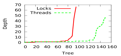
(a) Average depth of the tree nodes

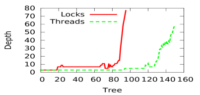
(b) Maximum depth of the trees

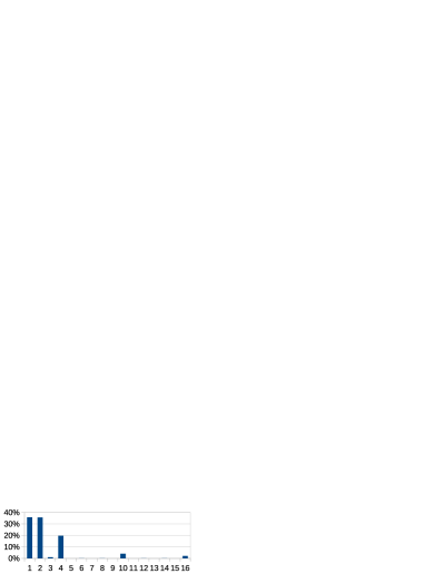
(c) Depth-distance frequency on causality queries

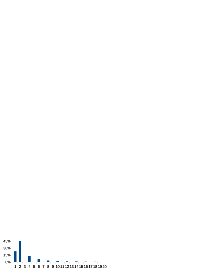
(d) Depth-distance frequency on conflict queries

Figure 3: (a), (b): depths of trees; (c), (d): frequency of depth distances

We run Dpu with an optimal exploration over 15 selected programs from Sec. 6.1, with 380 to 204K maximal configurations in the unfolding. In total, the 15 unfoldings contain 246 trees (150 thread trees and 96 lock trees) with 5.2M nodes. Fig. 3 shows the average depth of the nodes in each tree (subfigure a) and the maximum depth of the trees (subfigure b), for each of the 246 trees.

While the average depth of a node is 22.7, as much as 80% of the trees have a maximum depth of less than 8 nodes, and 90% of them less than 16 nodes. The average of 22.7 is however larger because deeper trees contain proportionally more nodes. The depth of the deepest node of every tree was between 3 and 77.

We next evaluate depth differences in the causality and conflict queries over these trees. Fig. 3 (a) and (b) respectively show the frequency of various depth distances associated to causality and conflict queries made by optimal POR.

Surprisingly, depth differences are very small for both causality and conflict queries. When deciding causality between events, as much as 92% of the queries were for tree nodes separated by a distance between 1 and 4, and 70% had a difference of 1 or 2 nodes. This means that optimal POR, and specifically the procedure that adds $\mathop{\mathit{ex}}(C)$ to the unfolding (which is the main source of causality queries), systematically performs causality queries which are trivial with the proposed data structures. The situation is similar for checking conflicts: 82% of the queries are about tree nodes whose depth difference is between 1 and 4.

Table 2: Comparing DPU with Maple (same machine). LOC: lines of code; Execs: nr. of executions; R: safe or unsafe. Other columns as before. Timeout: 8 min.

These experiments show that most queries on the causality trees require very short walks, which strongly drives to use the data structure proposed in Sec. 5. Finally, we chose a (rather arbitrary) skip step of 4. We observed that other values do not significantly impact the run time/memory consumption for most benchmarks, since the depth difference on causality/conflict requests is very low.

6.3 Evaluation Against the State-of-the-art on System Code

We now evaluate the scalability and applicability of Dpu on five multithreaded programs in two Debian packages:  blktrace [5], a block layer I/O tracing mechanism, and  mafft [12], a tool for multiple alignment of amino acid or nucleotide sequences. The code size of these utilities ranges from 2K to 40K LOC, and mafft is parametric in the number of threads.

We compared Dpu against Maple [24], a state-of-the-art testing tool for multithreaded programs, as the top ranked verification tools from SVCOMP’17 are still unable to cope with such large and complex multithreaded code. Unfortunately we could not compare against Nidhugg because it cannot deal with the (abundant) C-library calls in these programs.

Section 6.1 presents our experimental results. We use Dpu with optimal exploration and the modified version of Maple used in [22]. To test the effectiveness of both approaches in state space coverage and bug finding, we introduce bugs in 4 of the benchmarks (Add,Dnd,Mdl,pla). For the safe benchmark Blk, we perform exhaustive state-space exploration using Maple’s DFS mode. On this benchmark, Dpu outperfors Maple by several orders of magnitude: Dpu explores up to 20K executions covering the entire state space in 10s, while Maple only explores up to 108 executions in 8 min.

For the remaining benchmarks, we use the random scheduler of Maple, considered to be the best baseline for bug finding [22]. First, we run Dpu to retrieve a bound on the number of random executions to answer whether both tools are able to find the bug within the same number of executions. Maple found bugs in all buggy programs (except for one variant in Add) even though Dpu greatly outperforms and is able to achieve much more state space coverage.

6.4 Profiling a Stateless POR

In order to understand the cost of each component of the algorithm, we profile Dpu on a selection of 7 programs from Sec. 6.1. Dpu spends between 30% and 90% of the run time executing the program (65% in average). The remaining time is spent computing alternatives, distributed as follows: adding events to the event structure (15% to 30%), building the spikes of a new comb (1% to 50%), searching for solutions in the comb (less than 5%), and computing conflicting extensions (less than 5%). Counterintuitively, building the comb is more expensive than exploring it, even in the optimal case. Filling the spikes seems to be more memory-intensive than exploring the comb, which exploits data locality.

7 Conclusion

We have shown that computing alternatives in an optimal DPOR exploration is NP-complete. To mitigate this problem, we introduced a new approach to compute alternatives in polynomial time, approximating the optimal exploration with a user-defined constant. Experiments conducted on benchmarks including Debian packages show that our implementation outperforms current verification tools and uses appropriate data structures. Our profiling results show that running the program is often more expensive than computing alternatives. Hence, efforts in reducing the number of redundant executions, even if significantly costly, are likely to reduce the overall execution time.

Appendix 0.A Additional Basic Definitions

In this section we introduce a number of definitions that were excluded from the body of the paper owing to space constraints.

Labelled Transition Systems.

We defined an $LTS$ semantics for programs in Sec. 2 without first providing a general definition of $LTS$s. An $LTS$ [CGP99] is a structure $M\mathrel{:=}\langle\Sigma,\to,A,s_{0}\rangle$, where $\Sigma$ are the states, $A$ the actions, ${\to}\subseteq\Sigma\times A\times\Sigma$ the transition relation, and $s_{0}\in\Sigma$ an initial state. If $s\mathrel{\raisebox{-1.9pt}{$\xrightarrow{a}$}}s^{\prime}$ is a transition, the action $a$ is enabled at $s$ and $a$ can fire at $s$ to produce $s^{\prime}$. We let $\mathop{\mathit{enabl}}(s)$ denote the set of actions enabled at $s$.

A sequence $\sigma\mathrel{:=}a_{1}\ldots a_{n}\in A^{*}$ is a run when there are states $s_{1},\ldots,s_{n}$ satisfying $s_{0}\mathrel{\raisebox{-1.9pt}{$\xrightarrow{a_{1}}$}}s_{1}\ldots\mathrel{\raisebox{-1.9pt}{$\xrightarrow{a_{n}}$}}s_{n}$. We define $\mathop{\mathit{state}}(\sigma)\mathrel{:=}s_{n}$. We let $\mathop{\mathit{runs}}(M)$ denote the set of all runs of $M$, and $\mathop{\mathit{reach}}(M)\mathrel{:=}{\{\mathop{\mathit{state}}(\sigma)\in\Sigma\colon\sigma\in\mathop{\mathit{runs}}(M)\mathclose{\}}}$ the set of all reachable states.

Prime Event Structures.

Let $\mathcal{E}\mathrel{:=}\langle E,{<},{\mathrel{\#}}\rangle$ be a pes. Two events $e,e^{\prime}\in E$ are in immediate conflict if $e\mathrel{\#}e^{\prime}$ but both $\left\lceil e\right\rceil\cup[e]$ and $[e]\cup\left\lceil e^{\prime}\right\rceil$ are free of conflict. Given a set $U\subseteq E$, we denote by $\mathop{\mathit{\#^{i}_{U}}}(e)$ the set of events in $U$ that are in immediate conflict with $e$.

Unfolding semantics of an $LTS$.

In Sec. 2 we defined the unfolding semantics of a program (Def. 1). Now we give a slightly more general definition for $LTS$s instead of programs. The definitions are almost identical, the only differences are found in the first three lines of the definition. In particular the four fixpoint rules are exactly the same. The reason why we give now this definition over $LTS$ is because we will use it to define unfolding semantics for Petri nets in the proof of Theorem 4.3.

Definition 8 (Unfolding of an $LTS$ [19])

Given an $LTS$ $M\mathrel{:=}\langle\Sigma,\to,A,s_{0}\rangle$ and some independence relation ${\mathrel{\diamondsuit}}\subseteq A\times A$ on $M$, the unfolding of $M$ under $\mathrel{\diamondsuit}$, denoted $\mathcal{U}_{M,\mathrel{\diamondsuit}}$, is the pes over $A$ constructed by the following fixpoint rules:

1. Start with a pes $\mathcal{E}\mathrel{:=}\langle E,<,{\mathrel{\#}},h\rangle$ equal to $\langle\emptyset,\emptyset,\emptyset,\emptyset\rangle$.

2. Add a new event $e\mathrel{:=}\langle a,C\rangle$ to $E$ for any configuration $C\in\mathop{\mathit{conf}}(\mathcal{E})$ and any action $a\in A$ such that $a$ is enabled at $\mathop{\mathit{state}}(C)$ and $\lnot(a\mathrel{\diamondsuit}h(e^{\prime}))$ holds for every $<$-maximal event $e^{\prime}$ in $C$.

3. For any new $e$ in $E$, update $<$, $\mathrel{\#}$, and $h$ as follows:

   • for every $e^{\prime}\in C$, set $e^{\prime}<e$;

   • for any $e^{\prime}\in E\setminus C$, set $e^{\prime}\mathrel{\#}e$ if $e\neq e^{\prime}$ and $\lnot(a\mathrel{\diamondsuit}h(e^{\prime}))$;

   • set $h(e)\mathrel{:=}a$.

4. Repeat steps 2 and 3 until no new event can be added to $E$; return $\mathcal{E}$.

Obviously, both Def. 1 and Def. 8 produce the same unfolding when applied to a program. That is, for any program $P$ and independence $\mathrel{\diamondsuit}$ on $M_{P}$, we have that $\mathcal{U}_{P,\mathrel{\diamondsuit}}$ (Def. 1) is equal to $\mathcal{U}_{M_{P},\mathrel{\diamondsuit}}$ (Def. 8).

Petri nets.

A Petri net [Mur89] is a model of a concurrent system. Formally, a net is a tuple $N\mathrel{:=}\langle P,T,F,m_{0}\rangle$, where $P$ and $T$ are disjoint finite sets of places and transitions, $F\subseteq(P\times T)\cup(T\times P)$ is the flow relation, and $m_{0}\colon P\to\mathbb{N}$ is the initial marking. $N$ is called finite if $P$ and $T$ are finite. Places and transitions together are called nodes.

For $x\in P\cup T$, let ${}^{\bullet}x\mathrel{:=}\{y\in P\cup T\colon(y,x)\in F\}$ be the preset, and $x^{\bullet}\mathrel{:=}\{y\in P\cup T\colon(x,y)\in F\}$ the postset of $x$. The state of a net is represented by a marking. A marking of $N$ is a function $m\colon P\to\mathbb{N}$ that assigns tokens to every place. A transition $t$ is enabled at a marking $m$ iff for any $p\in{}^{\bullet}t$ we have $m(p)\geq 1$.

We give semantics to nets using transition systems. We associate $N$ with a transition system $M_{N}\mathrel{:=}\langle\Sigma,{\to},A,m_{0}\rangle$ where $\Sigma\mathrel{:=}P\to\mathbb{N}$ is the set of markings, $A\mathrel{:=}T$ is the set of transitions, and ${\to}\subseteq\Sigma\times A\times\Sigma$ contains a triple $m\mathrel{\raisebox{-1.9pt}{$\xrightarrow{t}$}}m^{\prime}$ exactly when, for any $p\in{}^{\bullet}t$ we have $m(p)\geq 1$, and for any $p\in P$ we have $m^{\prime}(p)=m(p)-|{\{p\mathclose{\}}}\cap{}^{\bullet}t|+|{\{p\mathclose{\}}}\cap t^{\bullet}|$. We call $N$ $k$-safe when for any reachable marking $m\in\mathop{\mathit{reach}}(M_{N})$ we have $m(p)\leq k$, for $p\in P$.

Appendix 0.B General Lemmas

For the rest of this section, we fix an $LTS$ $M\mathrel{:=}\langle\Sigma,A,{\to},s_{0}\rangle$ and an independence relation $\mathrel{\diamondsuit}$ on $M$. We assume that $\mathop{\mathit{runs}}(M)$ is a finite set of finite sequences. Let $\mathcal{U}_{M,\mathrel{\diamondsuit}}\mathrel{:=}\langle E,<,{\mathrel{\#}},h\rangle$ be the unfolding of $M$ under $\mathrel{\diamondsuit}$, which we will abbreviate as $\mathcal{U}$. Note that $\mathcal{U}$ is finite because of our assumption about $\mathop{\mathit{runs}}(M)$. We assume that $\mathcal{U}$ is the input pes provided to Alg. 1. Finally, without loss of generality we assume that $\mathcal{U}$ contains a special event $\bot$ that is a causal predecessor of any other event in $\mathcal{U}$.

Algorithm 1 is recursive, each call to Explore($C,D,A$) yields either no recursive call, if the function returns at Alg. 1, or one single recursive call (Alg. 1), or two (Alg. 1 and Alg. 1). Furthermore, it is non-deterministic, as $e$ is chosen from either the set $\mathop{\mathit{en}}(C)\setminus D$ or the set $A\cap\mathop{\mathit{en}}(C)$, which in general are not singletons. As a result, the configurations explored by it may differ from one execution to the next.

For each run of the algorithm on $\mathcal{U}$ we define the call graph explored by Alg. 1 on that run as a directed graph $\langle B,{\mathrel{\triangleright}}\rangle$ representing the actual exploration of $\mathcal{U}$. Different executions will in general yield different call graphs.

The nodes $B$ of the call graph are 4-tuples of the form $\langle C,D,A,e\rangle$, where $C,D,A$ are the parameters of a recursive call made to the funtion Explore($\cdot,\cdot,\cdot$), and $e$ is the event selected by the algorithm immediately before Alg. 1. More formally, $B$ contains exactly all tuples $\langle C,D,A,e\rangle$ satisfying that

• $C$, $D$, and $A$ are sets of events of the unfolding $\mathcal{U}$;

• during the execution of Explore($\emptyset,\emptyset,\emptyset$), the function Explore($\cdot,\cdot,\cdot$) has been recursively called with $C,D,A$ as, respectively, first, second, and third argument;

• $e\in E$ is the event selected by Explore($C,D,A$) immediately before Alg. 1 if $\mathop{\mathit{en}}(C)\not\subseteq D$. When $\mathop{\mathit{en}}(C)\subseteq D$ we define $e\mathrel{:=}\bot$.

The edge relation of the call graph, ${\mathrel{\triangleright}}\subseteq B\times B$, represents the recursive calls made by Explore($\cdot,\cdot,\cdot$). Formally, it is the union of two disjoint relations ${\mathrel{\triangleright}}\mathrel{:=}{\mathrel{\triangleright_{l}}}\uplus{\mathrel{\triangleright_{r}}}$, defined as follows. We define that

$$\langle C,D,A,e\rangle\mathrel{\triangleright_{l}}\langle C^{\prime},D^{\prime},A^{\prime},e^{\prime}\rangle\text{ ~{} and that ~{} }\langle C,D,A,e\rangle\mathrel{\triangleright_{r}}\langle C^{\prime\prime},D^{\prime\prime},A^{\prime\prime},e^{\prime\prime}\rangle$$

iff the execution of Explore($C,D,A$) issues a recursive call to, respectively, Explore($C^{\prime},D^{\prime},A^{\prime}$) at Alg. 1 and Explore($C^{\prime\prime},D^{\prime\prime},A^{\prime\prime}$) at Alg. 1. Observe that $C^{\prime}$ and $C^{\prime\prime}$ will necessarily be different (as $C^{\prime}=C\cup{\{e\mathclose{\}}}$, where $e\notin C$, and $C^{\prime\prime}=C$), and therefore the two relations are disjoint sets. We distinguish the node

$$b_{0}\mathrel{:=}\langle\emptyset,\emptyset,\emptyset,\bot\rangle$$

as the initial node, also called the root node. Observe that $\langle B,{\mathrel{\triangleright}}\rangle$ is by definition a weakly connected digraph, as there is a path from the node $b_{0}$ to every other node in $B$. We refer to $\mathrel{\triangleright_{l}}$ as the left-child relation and $\mathrel{\triangleright_{r}}$ as the right child relation.

Lemma 1

Let $\langle C,D,A,e\rangle\in B$ be a state of the call graph. We have that

• $D\cap A=\emptyset$; (1)

• event $e$ is such that $e\in\mathop{\mathit{en}}(C)\setminus D$; (2)

• $C$ is a configuration; (3)

• $C\cup A$ is a configuration and $C\cap A=\emptyset$; (4)

• $D\subseteq\mathop{\mathit{ex}}(C)$; (5)

Proof

Proving • ‣ Lemma 1 is immediate, assuming that • ‣ Lemma 1 holds. In Alg. 1, observe both branches of the conditional statement where $e$ is selected. If $e$ is slected by the then branch, clearly $e\in\mathop{\mathit{en}}(C)\setminus D$. If $e$ is selected by the else branch, clearly $e\in\mathop{\mathit{en}}(C)$. But, by • ‣ Lemma 1 $e\notin D$, as $e\in A$ and $A$ is disjoint with $D$. Therefore $e\in\mathop{\mathit{en}}(C)\setminus D$. In both cases • ‣ Lemma 1 holds, what we wanted to prove.

All remaining items, • ‣ Lemmas 1, • ‣ 1, • ‣ 1 and • ‣ 1, will be shown by induction on the length $n\geq 0$ of any path

$$b_{0}\mathrel{\triangleright}b_{1}\mathrel{\triangleright}\ldots\mathrel{\triangleright}b_{n-1}\mathrel{\triangleright}b_{n}$$

on the call graph, starting from the initial node and leading to $b_{n}\mathrel{:=}\langle C,D,A,e\rangle$ For $i\in{\{0,\ldots,n\mathclose{\}}}$ we define $\langle C_{i},D_{i},A_{i},e_{i}\rangle\mathrel{:=}b_{i}$.

We start showing • ‣ Lemma 1. Base case. $n=0$ and $D=A=\emptyset$. The result holds. Step. Assume that $D_{n-1}\cap A_{n-1}=\emptyset$ holds. We have

$$D\cap A=D_{n}\cap A_{n}=D_{n-1}\cap(A_{n-1}\setminus{\{e\mathclose{\}}})=D_{n-1}\cap A_{n-1}=\emptyset$$

because removing event $e$ from $A$ will not increase the number of events shared by $A$ and $D$.

We now show • ‣ Lemma 1, also by induction on $n$. Base case. $n=0$ and $C=\emptyset$. The set $\emptyset$ is a configuration. Step. Assume $C_{n-1}$ is a configuration. If $b_{n-1}\mathrel{\triangleright_{l}}b_{n}$, then $C=C_{n-1}\cup{\{e\mathclose{\}}}$ for some event $e\in\mathop{\mathit{en}}(C)$, as stated in • ‣ Lemma 1. By definition, $C$ is a configuration. If $b_{n-1}\mathrel{\triangleright_{r}}b_{n}$, then $C=C_{n-1}$. In any case $C$ is a configuration.

We show • ‣ Lemma 1, by induction on $n$. Base case. $n=0$. Then $C=\emptyset$ and $A=\emptyset$. Clearly $C\cup A$ is a configuration and $C\cup A=\emptyset$. Step. Assume that $C_{n-1}\cup A_{n-1}$ is a configuration and that $C_{n-1}\cap A_{n-1}=\emptyset$. We have two cases.

• Assume that $b_{n-1}\mathrel{\triangleright_{l}}b_{n}$. If $A_{n-1}$ is empty, then $A$ is empty as well. Clearly $C\cup A$ is a configuration and $C\cap A$ is empty. If $A_{n-1}$ is not empty, then $C=C_{n-1}\cup{\{e\mathclose{\}}}$ and $A=A_{n-1}\setminus{\{e\mathclose{\}}}$, for some $e\in A_{n-1}$, and we have

  $$C\cup A=(C_{n-1}\cup{\{e\mathclose{\}}})\cup(A_{n-1}\setminus{\{e\mathclose{\}}})=C_{n-1}\cup A_{n-1},$$

  so $C\cup A$ is a configuration as well. We also have that $C\cap A=C_{n-1}\cap A_{n-1}$ (recall that $e\notin C$), so $C\cap A$ is empty.

• Assume that $b_{n-1}\mathrel{\triangleright_{r}}b_{n}$ holds. Then we have $C=C_{n-1}$ and also $A=J\setminus C_{n-1}$ for some $J\in\textnormal{{Alt(}}\textnormal{\emph{$C_{n-1},D\cup{\{e\mathclose{\}}}$}}\textnormal{{)}}$. Since $J$ is a clue, from Defs. 3 and 2, we know that $C_{n-1}\cup J$ is a configuration. As a result,

  $$C\cup A=C_{n-1}\cup(J\setminus C_{n-1})=C_{n-1}\cup J,$$

  and therefore $C\cup A$ is a configuration. Finally, by construction of $A$ at Alg. 1, we clearly have $C\cap A=\emptyset$.

We show • ‣ Lemma 1, again, by induction on $n$. Base case. $n=0$ and $D=\emptyset$. Then • ‣ Lemma 1 clearly holds. Step. Assume that • ‣ Lemma 1 holds for $\langle C_{i},D_{i},A_{i},e_{i}\rangle$, with $i\in{\{0,\ldots,n-1\mathclose{\}}}$. We show that it holds for $b_{n}$. As before, we have two cases.

• Assume that $b_{n-1}\mathrel{\triangleright_{l}}b_{n}$. We have that $D=D_{n-1}$ and that $C=C_{n-1}\cup{\{e_{n-1}\mathclose{\}}}$. We need to show that for all $e^{\prime}\in D$ we have $\left\lceil e^{\prime}\right\rceil\subseteq C$ and $e^{\prime}\notin C$. By induction hypothesis we know that $D=D_{n-1}\subseteq\mathop{\mathit{ex}}(C_{n-1})$, so clearly $\left\lceil e^{\prime}\right\rceil\subseteq C_{n-1}\subseteq C$. We also have that $e^{\prime}\notin C_{n-1}$, so we only need to check that $e^{\prime}\neq e_{n-1}$. By • ‣ Lemma 1 applied to $b_{n-1}$ we have that $e_{n-1}\notin D_{n-1}=D$. That means that $e^{\prime}\neq e_{n-1}$.

• Assume that $b_{n-1}\mathrel{\triangleright_{r}}b_{n}$. We have that $D=D_{n-1}\cup{\{e_{n-1}\mathclose{\}}}$, and by hypothesis we know that $D_{n-1}\subseteq\mathop{\mathit{ex}}(C_{n-1})=\mathop{\mathit{ex}}(C)$. As for $e_{n-1}$, by • ‣ Lemma 1 we know that $e_{n-1}\in\mathop{\mathit{en}}(C_{n-1})=\mathop{\mathit{en}}(C)\subseteq\mathop{\mathit{ex}}(C)$. As a result, $D\subseteq\mathop{\mathit{ex}}(C)$.

Lemma 2

Let $b\mathrel{:=}\langle C,D,A,e\rangle$ and $b^{\prime}\mathrel{:=}\langle C^{\prime},D^{\prime},A^{\prime},e^{\prime}\rangle$ be two nodes of the call graph such that $b\mathrel{\triangleright}b^{\prime}$. Then

• $C\subseteq C^{\prime}$ and $D\subseteq D^{\prime}$; (6)

• if $b\mathrel{\triangleright_{l}}b^{\prime}$, then $C\subsetneq C^{\prime}$; (7)

• if $b\mathrel{\triangleright_{r}}b^{\prime}$, then $D\subsetneq D^{\prime}$. (8)

Proof

If $b\mathrel{\triangleright_{l}}b^{\prime}$, then $C^{\prime}=C\cup{\{e\mathclose{\}}}$ and $D^{\prime}=D$. Then all the three statements hold. If $b\mathrel{\triangleright_{r}}b^{\prime}$, then $C^{\prime}=C$ and $D^{\prime}=D\cup{\{e\mathclose{\}}}$. Similarly, all the three statements hold.

Lemma 3

If $C\subseteq C^{\prime}$ are two finite configurations, then $\mathop{\mathit{en}}(C)\cap(C^{\prime}\setminus C)=\emptyset$ iff $C^{\prime}\setminus C=\emptyset$.

Proof

If there is some $e\in\mathop{\mathit{en}}(C)\cap(C^{\prime}\setminus C)$, then $e\notin C$ and $e\in C^{\prime}$, so $C^{\prime}\setminus C$ is not empty. If there is some $e^{\prime}\in C^{\prime}\setminus C$, then there is some $e^{\prime\prime}$ event that is $<$-minimal in $C^{\prime}\setminus C$. As a result, $\left\lceil e^{\prime\prime}\right\rceil\subseteq C$. Since $e^{\prime\prime}\notin C$ and $C\cup{\{e^{\prime\prime}\mathclose{\}}}$ is a configuration (as $C\cup{\{e^{\prime\prime}\mathclose{\}}}\subseteq C^{\prime}$), we have that $e^{\prime\prime}\in\mathop{\mathit{en}}(C)$. Then $\mathop{\mathit{en}}(C)\cap(C^{\prime}\setminus C)$ is not empty.

Appendix 0.C Termination Proofs

Lemma 4

Any path $b_{0}\mathrel{\triangleright}b_{1}\mathrel{\triangleright}b_{2}\mathrel{\triangleright}\ldots$ in the call graph starting from $b_{0}$ is finite.

Proof

By contradiction. Assume that $b_{0}\mathrel{\triangleright}b_{1}\mathrel{\triangleright}\ldots$ is an infinite path in the call graph. For $0\leq i$, let $\langle C_{i},D_{i},A_{i},e_{i}\rangle\mathrel{:=}b_{i}$. Recall that $\mathcal{U}$ has finitely many events, finitely many finite configurations, and no infinite configuration. Now, observe that the number of times that $C_{i}$ and $C_{i+1}$ are related by $\mathrel{\triangleright_{l}}$ rather than $\mathrel{\triangleright_{r}}$ is finite, since every time Explore($\cdot,\cdot,\cdot$) makes a recursive call at Alg. 1 it adds one event to $C_{i}$, as stated by • ‣ Lemma 2. More formally, the set

$$L\mathrel{:=}{\{i\in\mathbb{N}\colon C_{i}\mathrel{\triangleright_{l}}C_{i+1}\mathclose{\}}}$$

is finite. As a result it has a maximum, and its successor $k\mathrel{:=}1+\max_{<}L$ is an index in the path such that for all $i\geq k$ we have $C_{i}\mathrel{\triangleright_{r}}C_{i+1}$, i.e., the function only makes recursive calls at Alg. 1. We then have that $C_{i}=C_{k}$, for $i\geq k$, and by • ‣ Lemma 1, that $D_{i}\subseteq\mathop{\mathit{ex}}(C_{k})$. Since $\mathcal{U}$ is finite, note that $\mathop{\mathit{ex}}(C_{k})$ is finite as well. But, as a result of • ‣ Lemma 2 the sequence

$$D_{k}\subsetneq D_{k+1}\subsetneq D_{k+2}\subsetneq\ldots$$

is an infinite increasing sequence. This is a contradiction, as for sufficiently large $j\geq 0$ we will have that $D_{k+j}$ will be larger than $\mathop{\mathit{ex}}(C_{k})$, yet $D_{k+j}\subseteq\mathop{\mathit{ex}}(C_{k})$.

See 3.1

Proof

The statement of the theorem refers to Alg. 1, but we instead prove it for Alg. 1. Remark that Alg. 1 makes calls to two functions, namely, Remove($\cdot$) and Alt($\cdot,\cdot$). Clearly both of them terminate (the loop in Remove($\cdot$) iterates over a finite set). Since we gave no algorithm to compute Alt($\cdot$), we will assume we employ one that terminates on every input.

Now, observe that there is no loop in Alg. 1. Thus any non-terminating execution of Alg. 1 must perform a non-terminating sequence of recursive calls, which entails the existence of an infinite path in the call graph associated to the execution. Since, by Lemma 4, no infinite path exist in the call graph, Alg. 1 always terminates.

Appendix 0.D Completeness Proofs

Lemma 5

Let $b\mathrel{:=}\langle C,D,A,e\rangle\in B$ be a node in the call graph and $\hat{C}\subseteq E$ an arbitrary maximal configuration of $\mathcal{U}$ such that $C\subseteq\hat{C}$ and $D\cap\hat{C}=\emptyset$. Then exactly one of the following statements holds:

• Either $C$ is a maximal configuration of $\mathcal{U}$, or

• $C$ is not maximal but $\mathop{\mathit{en}}(C)\subseteq D$, or

• $e\in\hat{C}$ and $b$ has a left child, or

• $e\notin\hat{C}$ and $b$ has a right child.

Proof

If $C$ is maximal, then the first statement holds and $b$ has no successor in the call graph, so none of the other three statements hold and we are done.

So assume that $C$ is not maximal. Then $\mathop{\mathit{en}}(C)\neq\emptyset$. Now, if $\mathop{\mathit{en}}(C)\subseteq D$ holds then the second statement is true and none of the others is (as Alg. 1 does not make any recursive call in this case).

So assume also that $\mathop{\mathit{en}}(C)\not\subseteq D$. That implies that $b$ has at least one left child. If $e\in\hat{C}$, then we are done, as the second statement holds and none of the others hold.

So finally, assume that $e\notin\hat{C}$, we need to show that the third statement holds, i.e. that $b$ has right child. By Def. 3 we know that the set of clues returned by the call to Alt($C,D\cup{\{e\mathclose{\}}}$) will be non-empty, as there exists a maximal configuration $\hat{C}$ such that $C\subseteq\hat{C}$ (by hypothesis) and

$$\hat{C}\cap(D\cup{\{e\mathclose{\}}})=(\hat{C}\cap D)\cup(\hat{C}\cap{\{e\mathclose{\}}})=\hat{C}\cap D=\emptyset.$$

This means that Alg. 1 will make a recursive call at line Alg. 1 and $b$ will have a right child. This shows that the last statement holds. And clearly none of the other statements holds in this case.

Lemma 6

For any node $b\mathrel{:=}\langle C,D,\cdot,e\rangle\in B$ in the call graph and any maximal configuration $\hat{C}\subseteq E$ of $\mathcal{U}$, if

$$C\subseteq\hat{C}\text{ and }D\cap\hat{C}=\emptyset,$$

then there is a node $b^{\prime}\mathrel{:=}\langle C^{\prime},\cdot,\cdot,\cdot\rangle\in B$ such that $b\mathrel{\triangleright}^{*}b^{\prime}$ and $\hat{C}=C^{\prime}$.

Proof

The proof works by explicitly constructing a path from $b$ to $b^{\prime}$ using an iterated application of Lemma 5.

Since $C\subseteq\hat{C}$ and $D\cap\hat{C}=\emptyset$, we can apply Lemma 5 to $b$ and $\hat{C}$ and conclude that exactly one of the four statements in that Lemma will be true at $b$. If $C$ is maximal, then necessarily $C=\hat{C}$ and we are done. If $C$ is not maximal, then it must be the case that $\mathop{\mathit{en}}(C)\not\subseteq D$ and $b$ has at least one left child. This is because by Lemma 3 we have that

$$\mathop{\mathit{en}}(C)\cap(\hat{C}\setminus C)=\emptyset\text{ iff }\hat{C}\setminus C=\emptyset.$$

Since $C$ is not maximal $\hat{C}\setminus C\neq\emptyset$ and we see that $\mathop{\mathit{en}}(C)\cap\hat{C}$ must be non-empty. Now, since $\hat{C}$ and $D$ are disjoint, the event(s) in $\mathop{\mathit{en}}(C)\cap\hat{C}$ are not in $D$, and so $\mathop{\mathit{en}}(C)$ contains events which are not contained in $D$.

Since $\mathop{\mathit{en}}(C)\not\subseteq D$ we have that the second statement in Lemma 5 does not hold, and so either the third or the fourth statement have to be hold.

Now, $b$ has a left child and two cases are possible, either $e\in\hat{C}$ or not. If $e\in\hat{C}$ we let $b_{1}\mathrel{:=}\langle C_{1},D_{1},\cdot,e_{1}\rangle$ be the left child of $b$, with $C_{1}\mathrel{:=}C\cup{\{e\mathclose{\}}}$ and $D_{1}\mathrel{:=}D$. If $e\notin\hat{C}$, then only the last statement of Lemma 5 can hold and we know that $b$ has a right child. Let $b_{1}\mathrel{:=}\langle C_{1},D_{1},\cdot,e_{1}\rangle$, with $C_{1}\mathrel{:=}C$ and $D_{1}\mathrel{:=}D\cup{\{e\mathclose{\}}}$ be that child. Observe that in both cases $C_{1}\subseteq\hat{C}$ and $D_{1}\cap\hat{C}=\emptyset$.

If $C_{1}$ is maximal, then necessarily $C_{1}=\hat{C}$, we take $b^{\prime}\mathrel{:=}b_{1}$ and we have finished. If not, we can reapply Lemma 5 at $b_{1}$ and make one more step into one of the children $b_{2}$ of $b_{1}$. If $C_{2}$ is still not maximal (thus different from $\hat{C}$) we need to repeat the argument starting from $b_{2}$ only a finite number $n$ of times until we reach a node $b_{n}\mathrel{:=}\langle C_{n},D_{n},\cdot,\cdot\rangle$ where $C_{n}$ is a maximal configuration. This is because every time we repeat the argument on a non-maximal node $b_{i}$ we advance one step down in the call graph, and by Lemma 4 all paths in the graph starting from the root are finite. So eventually we find a leaf node $b_{n}$ where $C_{n}$ is maximal and satisfies $C_{n}\subseteq\hat{C}$. This implies that $C_{n}=\hat{C}$, and we can take $b^{\prime}\mathrel{:=}b_{n}$.

See 3.2

Proof

We need to show that for every maximal configuration $\hat{C}\subseteq E$ we can find a node $b\mathrel{:=}\langle C,\cdot,\cdot,\cdot\rangle$ in $B$ such that $\hat{C}=C$. This is a direct consequence of Lemma 6. Consider the root node of the tree, $b_{0}\mathrel{:=}\langle C_{0},D_{0},A_{0},\bot\rangle$, where $C_{0}=D_{0}=A_{0}=\emptyset$. Clearly $C_{0}\subseteq\hat{C}$ and $D_{0}\cap\hat{C}=\emptyset$, so Lemma 6 applies to $\hat{C}$ and $b_{0}$, and establishes the existence of the aforementioned node $b$.

Appendix 0.E Complexity Proofs

See 4.1

Proof

We first prove that the problem is in NP. Let us non-deterministically choose a configuration $J\subseteq E$. We then check that $J$ is an alternative to $D$ after $C$:

• $J\cup C$ is a configuration can be checked in linear time: The first condition for $J\cup C$ to be a configuration is that $\forall e\in J\cup C:\left\lceil e\right\rceil\subseteq J\cup C$. Since $J$ is a configuration, this condition holds for all $e\in J$. Similarly, as $C$ is a configuration, it also holds for all $e\in C$. The second condition is that $\forall e_{1},e_{2}\in J\cup C:\lnot(e_{1}\mathrel{\#}e_{2})$. This is true for $e_{1},e_{2}\in J$ and $e_{1},e_{2}\in C$. If $e_{1}\in J\land e_{2}\in C$ (or the converse), we have to effectively check that $\lnot(e_{1}\mathrel{\#}e_{2})$. Checking if two events $e_{1}$ and $e_{2}$ are in conflict is linear on the size of $[e_{1}]\cup[e_{2}]$.

• Every event $e_{1}\in D$ must be in immediate conflict with an event $e_{2}\in J$. Thus, there are at most $|D|\cdot|J|$ checks to perform, each in linear time on the size of $[e_{1}]\cup[e_{2}]$. Hence, this is in $O(n^{2})$.

We now prove that the problem is NP-hard, by reduction from the 3-SAT problem. Let ${\{v_{1},\ldots,v_{n}\mathclose{\}}}$ be a set of Boolean variables. Let $\phi\mathrel{:=}c_{1}\land\ldots\land c_{m}$ be a 3-SAT formula, where each clause $c_{i}\mathrel{:=}l_{i}\lor l^{\prime}_{i}\lor l^{\prime\prime}_{i}$ comprises three literals. A literal is either a Boolean variable $v_{i}$ or its negation $\overline{v_{i}}$.

Formula $\phi$ can be modelled by a PES $\mathcal{E}_{\phi}\mathrel{:=}\langle E,{<},\mathrel{\#},h\rangle$ constructed as follows:

• For each variable $v_{i}$ we create two events $t_{i}$ and $f_{i}$ in $E$, and put them in immediate conflict, as they correspond to the satisfaction of $v_{i}$ and $\overline{v_{i}}$, respectively.

• The set $D$ of events to disable contains one event $d_{j}$ per clause $c_{j}$. Such a $d_{j}$ has to be in immediate conflict with the events modelling the literals in clause $c_{j}$. Hence it is in conflict with 1, 2, or 3 $t$ or $f$ events.

• There is no causality: $<\mathrel{:=}\emptyset$.

• The labelling function shows the correspondence between the events and the elements of formula $\phi$, i.e. $\forall t_{i}\in E:h(t_{i})=v_{i}$, $\forall f_{i}\in E:h(f_{i})=\overline{v_{i}}$ and $\forall d_{j}\in E:h(d_{j})=c_{j}$.

We now show that $\phi$ is satisfiable iff there exists an alternative $J$ to $D$ after $C\mathrel{:=}\emptyset$ in $E$. This alternative is constructed by selecting for each event $d_{j}\in D$ and event $e$ in immediate conflict. By construction of $\mathcal{E}_{\phi}$, $h(e)$ is a literal in clause $h(d_{j})=c_{j}$. Moreover, $C\cup J=J$ must be a configuration. The causal closure is trivially satisfied since ${<}\mathrel{:=}\emptyset$. The conflict-freeness implies that if $t_{i}\in J$ then $f_{i}\not\in J$ and vice-versa. Therefore, formula $\phi$ is satisfiable iff an alternative $J$ to $D$ exists.

The construction of $\mathcal{E}_{\phi}$ is illustrated in Fig. 4 for: ϕ:=⏟(x_1 ∨$\overline{x_{2}}$ ∨x_3)_c_1 ∧⏟($\overline{x_{1}}$ ∨$\overline{x_{2}}$)_c_2 ∧⏟(x_1 ∨$\overline{x_{3}}$)_c_3

Figure 4: Example of encoding a 3-SAT formula.

See 4.2

Proof

Observe that the only difference between the statement of this theorem and that of Theorem 4.1 is that here we assume the PES to be the unfolding of a given program $P$ under the relation $\mathrel{\diamondsuit}_{P}$.

As a result the problem is obviously in NP, as restricting the class of PESs that we have as input cannot make the problem more complex.

However, showing that the problem is NP-hard requires a new encoding, as the (simple) encoding given for Theorem 4.1 generates PESs that may not be the unfolding of any program. Recall that two events in the unfolding of a program are in immediate conflict only if they are lock statements on the same variable. So, in Fig. 4, for instance, since $t_{1}\mathrel{\#}f_{1}$ and $f_{1}\mathrel{\#}d_{2}$, then necessarily we should have $t_{1}\mathrel{\#}d_{2}$, as all the three events should be locks to the same variable.

For this reason we give a new encoding of the 3-SAT problem into our problem. As before, let $V={\{v_{1},\ldots,v_{n}\mathclose{\}}}$ be a set of Boolean variables. Let $\phi\mathrel{:=}c_{1}\land\ldots\land c_{m}$ be a 3-SAT formula, where each clause $c_{i}\mathrel{:=}l_{i}\lor l^{\prime}_{i}\lor l^{\prime\prime}_{i}$ comprises three literals. A literal is either a Boolean variable $v_{i}$ or its negation $\overline{v_{i}}$. As before, for a variable $v$, let $\mathop{\mathit{pos}}(v)$ denote the set of clauses where $v$ appears positively and $\mathop{\mathit{neg}}(v)$ the set of clauses where it appears negated. We assume that every variable only appears either positively or negatively in a clause (or does not appear at all), as clauses where a variable happens both positively and negatively can be removed from $\phi$. As a result $\mathop{\mathit{pos}}(v)\cap\mathop{\mathit{neg}}(v)=\emptyset$ for every variable $v$.

Let us define a program $P_{\phi}$ as follows:

• For each Boolean variable $v_{i}$ we have two threads in $P$, $t_{i}$ corresponding to $v_{i}$ (true), and $f_{i}$ corresponding to $\overline{v_{i}}$ (false). We also have one lock $l_{v_{i}}$.

• Immediately after starting, both threads $t_{i}$ and $f_{i}$ lock on $l_{v_{i}}$. This scheme corresponds to choosing a Boolean value for variable $v_{i}$: the thread that locks first chooses the value of $v_{i}$.

• For each clause $c_{j}\in\phi$, we have a thread $d_{j}$ and a lock $l_{c_{j}}$. The thread contains only one statement which is locking $l_{c_{j}}$.

• For each clause $c_{j}\in\mathop{\mathit{pos}}(v_{i})\cup\mathop{\mathit{neg}}(v_{i})$, the program contains one thread $r_{\langle v_{i},c_{j}\rangle}$ (run for variable $v_{i}$ in clause $c_{j}$). This thread contains only one statement which is locking $l_{c_{j}}$.

• After locking on $l_{v_{i}}$, thread $t_{i}$ starts in a loop all threads $r_{\langle v_{i},c_{j}\rangle}$, for $c_{j}\in\mathop{\mathit{pos}}(v_{i})$. Since we do not have thread creation in our program model, we start a thread as follows: for each thread $r_{\langle v_{i},c_{j}\rangle}$ we create an additional lock that is initially acquired. Immediately after starting, $r_{\langle v_{i},c_{j}\rangle}$ tries to acquire it. When $t_{i}$ wishes to start the thread, it just releases the lock, effectively letting the thread start running.

• Similarly, after locking on $l_{v_{i}}$, thread $f_{i}$ starts in a loop all threads $r_{\langle v_{i},c_{j}\rangle}$, for $c_{j}\in\mathop{\mathit{neg}}(v_{i})$.

When $P_{\phi}$ is unfolded, each statement of the program gives rise to exactly one event in the unfolding. Indeed, by construction, each $t_{i}$ or $f_{i}$ thread starts by a lock event and then causally lead to one $r$ event per clause the variable $v_{i}$ appears in. Any two of them concern different clauses and thus different locks, and they are independent.

Let $C\mathrel{:=}\emptyset$ be an empty configuration, $D\mathrel{:=}{\{d_{1},\ldots,d_{m}\mathclose{\}}}$, and $U$ the set of all events in the unfolding of the program.

We now show that $\phi$ is satisfiable iff there exists an alternative $J$ to $D$ after $C\mathrel{:=}\emptyset$ in $\mathcal{U}_{P_{\phi},\mathrel{\diamondsuit}_{P_{\phi}}}$. This alternative is constructed by selecting for each event $d_{j}\in D$ and event $e$ in immediate conflict. By construction of $P_{\phi}$, it is a $r_{\langle v_{i},c_{j}\rangle}$ where $v_{i}$ is a literal in clause $h(d_{j})=c_{j}$. Moreover, $C\cup J=J$ must be a configuration. In order to satisfy the causal closure, since

$${<}\mathrel{:=}{\{\langle t_{i},r_{\langle v_{i},c_{j}\rangle}\rangle:c_{j}\in\mathop{\mathit{pos}}(v_{i})\mathclose{\}}}\cup{\{\langle f_{i},r_{\langle v_{i},c_{j}\rangle}\rangle:c_{j}\in\mathop{\mathit{neg}}(v_{i})\mathclose{\}}},$$

$J$ must also contain the $t_{i}$ or $f_{i}$ preceding $r_{\langle v_{i},c_{j}\rangle}$. The conflict-freeness implies that if $t_{i}\in J$ then $f_{i}\not\in J$ and vice-versa. Therefore, formula $\phi$ is satisfiable iff an alternative $J$ to $D$ exists.

There are at most $2|V|+|\phi|(|V|+1)$ events, so the construction can be achieved in polynomial time. Therefore our problem is NP-hard.

The construction of $\mathcal{U}_{P_{\phi}}$ is illustrated in Fig. 5 for: ϕ:=⏟(x_1 ∨$\overline{x_{2}}$ ∨x_3)_c_1 ∧⏟($\overline{x_{1}}$ ∨$\overline{x_{2}}$)_c_2 ∧⏟(x_1 ∨$\overline{x_{3}}$)_c_3

Figure 5: Program unfolding encoding a 3-SAT formula.

See 4.3

Proof

Given a Petri net $N\mathrel{:=}\langle P,T,F,m_{0}\rangle$, a transition $t\in T$, an independence relation ${\mathrel{\diamondsuit}}\subseteq T\times T$, the unfolding $\mathcal{E}\mathrel{:=}\mathcal{U}_{M_{N},\mathrel{\diamondsuit}}$ of $N$, and a configuration $C$ of $\mathcal{E}$, we need to prove that deciding whether $h^{-1}(t)\cap\mathop{\mathit{cex}}(C)=\emptyset$ is an NP-complete problem.

We first prove that the problem is in NP. This is achieved using a guess and check non-deterministic algorithm to decide the problem. Let us non-deterministically choose a configuration $C^{\prime}\subseteq C$, in linear time on the input. A linearisation of $C^{\prime}$ is chosen and used to compute the marking $m$ reached. We check that $m$ enables $t$ and that for any $<$-maximal event $e$ of $C$, $\lnot(h(e)\mathrel{\diamondsuit}t)$ holds. Both tests can be done in polynomial time. If both tests succeed then we answer yes, otherwise we answer no.

We now prove that the problem is NP-hard, by reduction from the 3-SAT problem. Let $V={\{v_{1},\ldots,v_{n}\mathclose{\}}}$ be a set of Boolean variables. Let $\phi\mathrel{:=}c_{1}\land\ldots\land c_{m}$ be a 3-SAT formula, where each clause $c_{i}\mathrel{:=}l_{i}\lor l^{\prime}_{i}\lor l^{\prime\prime}_{i}$ comprises three literals. A literal is either a Boolean variable $v_{i}$ or its negation $\overline{v_{i}}$. For a variable $v$, $\mathop{\mathit{pos}}(v)$ denotes the set of clauses where $v$ appears positively and $\mathop{\mathit{neg}}(v)$ the set of clauses where it appears negated.

Given $\phi$, we construct a $3$-safe net $N_{\phi}$, an independence relation $\mathrel{\diamondsuit}$, a configuration $C$ of the unfolding $\mathcal{E}$, and a transition $t$ from $N_{\phi}$ such that $\phi$ is satisfiable iff some event in $\mathop{\mathit{ex}}(C)$ is labelled by $t$ :

• The net contains one place $d_{i}$ per clause $c_{i}$, initially empty.

• For each variable $v_{i}$ are two places $s_{i}$ and $s^{\prime}_{i}$. Places $s_{i}$ initially contain $1$ token while places $s^{\prime}_{i}$ are empty.

• For each variable $v_{i}$, a transition $p_{i}$ takes into account positive values of the variable. It takes a token from $s_{i}$, puts one in $s^{\prime}_{i}$ (to move on to the other possibility for this variable) and puts one token in all places associated with clauses $c_{j}\in\mathop{\mathit{pos}}(v_{i})$. This transition mimics the validation of clauses where the variable appears as positive.

• For each variable $v_{i}$, a transition $n_{i}$ takes into account negative values of the variable. It takes a token from $s^{\prime}_{i}$ and puts one token in all places associated with clauses $c_{j}\in\mathop{\mathit{neg}}(v_{i})$. It also removes one token from all places associated with clauses $c_{j}\in\mathop{\mathit{pos}}(v_{i})$, that have been marked by some $p_{k}$ transition. This transition $n_{i}$ mimics the validation of clauses where the variable appears as negative.

• Finally, a transition $t$ is added that takes a token from all $d_{i}$. Thus, it can only be fired when all clauses are satisfied, i.e. formula $\phi$ is satisfied.

The independence relation $\mathrel{\diamondsuit}$ is the smallest binary, symmetric, irreflexive relation such that $p_{i}\mathrel{\diamondsuit}p_{j}$ exactly when $i\neq j$ and $p_{i}\mathrel{\diamondsuit}n_{j}$ exactly when $i\neq j$. Recall that $p_{i},n_{i}$ correspond to respectively to the positive and negative valuations of variable $v_{i}$. In other words, the dependence relation ${\mathrel{\mathbin{\text{\rotatebox[origin={c}]{45.0}{$\boxplus$}}}}}\mathrel{:=}T\times T\setminus{\mathrel{\diamondsuit}}$ is the reflexive closure of the set

$${\{\langle p_{i},n_{i}\rangle\colon 1\leq i\leq n\mathclose{\}}}\cup{\{\langle t,p_{i}\rangle\colon 1\leq i\leq n\mathclose{\}}}\cup{\{\langle t,n_{i}\rangle\colon 1\leq i\leq n\mathclose{\}}}$$

Relation $\mathrel{\diamondsuit}$ is an independence relation because:

• $\forall i\neq j$, transitions $p_{i}$ and $p_{j}$ do not share any input place ;

• $\forall i\neq j$, the intersection between $p_{i}^{\bullet}$ and ${}^{\bullet}n_{j}$ might not be empty, but $n_{j}$ is always preceded by (and thus enabled after) $p_{j}$ (and not $p_{i}$). So firing $p_{i}$ cannot enable, nor disable, $p_{j}$, and firing $p_{i}$ and $n_{j}$ in any order reaches the same state.

Finally, configuration $C$ contains exactly one event per $p_{i}$ and one per $n_{i}$, hence $2|V|$ events. This is because transition $n_{i}$ is dependent only of $p_{i}$, and independent of (thus concurrent to) any other transition in $C$. Thus formula $\phi$ has a model iff there is an event $e\in\mathop{\mathit{en}}(C)$ labelled by $t$. Indeed, initially only positive transitions $p_{i}$ are enabled that assign a positive value to their corresponding variable $v_{i}$. They add a token in all places $d_{j}$ such that $c_{j}\in\mathop{\mathit{pos}}(v_{i})$. Then, when a negative transition $n_{i}$ fires, it deletes the tokens from these $d_{j}$ that had been created by $p_{i}$ since the variable cannot allow for validating these clauses anymore. It also adds tokens in the $d_{k}$ such that $c_{k}\in\mathop{\mathit{neg}}(v_{i})$ since the clauses involving $\overline{v_{i}}$ now hold. Therefore, the number of tokens in a place $d_{j}$ is the number of variables (or their negation) that validate the associated clause. Formula $\phi$ is satisfied when all clauses hold at the same time, i.e. each clause is validated by at least one variable. Thus all places $d$ must contain at least one token (and enable $t$) for $\phi$ satisfaction.

The construction of $N_{\phi}$ is illustrated in Fig. 6 for: ϕ:=⏟(x_1 ∨$\overline{x_{2}}$ ∨x_3)_c_1 ∧⏟($\overline{x_{1}}$ ∨$\overline{x_{2}}$)_c_2 ∧⏟(x_1 ∨$\overline{x_{3}}$)_c_3

Figure 6: Petri Net encoding a 3-SAT formula.

Appendix 0.F Proofs for Causality Trees

See 5.1

Proof

Firstly, we show that $e<e^{\prime}$ holds iff $e=\mathop{\mathit{tmax}}(e^{\prime},i)\lor e<\mathop{\mathit{tmax}}(e^{\prime},i)$.

• Direction $\Rightarrow$. Assume that $e<e^{\prime}$. This implies that $e\in\lceil e^{\prime}\rceil$ and there must exist $\hat{e}\in[e^{\prime}]$ such that $\hat{e}=tmax(e^{\prime},i)$. Since both $e$ and $\hat{e}$ are events from thread $i$, and both are contained in $[e^{\prime}]$ they cannot be in conflict, but $\lnot(h(e)\mathrel{\diamondsuit}h(\hat{e}))$. Then either $e=\hat{e}$ or $e<\hat{e}$.

• Direction $\Leftarrow$. Let $\hat{e}\mathrel{:=}\mathop{\mathit{tmax}}(e^{\prime},i)$. Since $i\neq i^{\prime}$ we have that $\hat{e}\neq e^{\prime}$, and since $\hat{e}\in[e^{\prime}]$ we have that $\hat{e}<e^{\prime}$. Let $e\in\mathcal{E}$ be any event such that either $e=\hat{e}$ or $e<\hat{e}$. We then have $e\leqslant\hat{e}<e^{\prime}$, so clearly $e<e^{\prime}$.

Now we show that $e\mathrel{\#}e^{\prime}$ holds iff there is some $l\in\mathcal{L}$ such that $\mathop{\mathit{lmax}}(e,l)\mathrel{\#}\mathop{\mathit{lmax}}(e^{\prime},l)$.

• Direction $\Rightarrow$. Assume that $e\mathrel{\#}e^{\prime}$ holds. Then necessary there exist events $e_{1}^{\prime}\in[e]$ and $e_{2}^{\prime}\in[e^{\prime}]$ such that $e_{1}^{\prime}\mathrel{\#^{i}}e_{2}^{\prime}$. Since only lock events touching the same variable are able to create immediate conflicts, we obviously know that $\exists l\in\mathcal{L}:h(e_{1}^{\prime})=h(e_{2}^{\prime})=\langle\texttt{acq},l\rangle$. Since $e_{1}^{\prime}\in[e]$ then $\exists e_{1}\in[e]:\exists e_{1}=\mathop{\mathit{lmax}}(e,l)$. Similarly, $\exists e_{2}\in[e^{\prime}]:e_{2}=\mathop{\mathit{lmax}}(e^{\prime},l)$. Both $e_{1}$ and $e_{2}$ are $<$-maximal events, so $e_{1}^{\prime}<e_{1}$ or $e_{1}^{\prime}=e_{1}$ and $e_{2}<e_{2}^{\prime}$ or $e_{2}=e_{2}^{\prime}$. The conflict is inherited, having $e_{1}^{\prime}\mathrel{\#^{i}}e_{2}^{\prime}$ implies $e_{1}\mathrel{\#}e_{2}$.

• Direction $\Leftarrow$. Assume that there is some $l\in\mathcal{L}$ such that $\mathop{\mathit{lmax}}(e,l)\mathrel{\#}\mathop{\mathit{lmax}}(e^{\prime},l)$ and let $e_{1}\in[e]:e_{1}=\mathop{\mathit{lmax}}(e,l)$ and $e_{2}\in[e^{\prime}]:e_{2}=\mathop{\mathit{lmax}}(e^{\prime},l)$, then $e_{1}\mathrel{\#}e_{2}$. Since $e_{1}\in[e]$, we have $e_{1}<[e]$. Similarly, $e_{2}\in[e^{\prime}]$, i.e., $e_{2}<e^{\prime}$. The conflict is inherited and $e_{1}\mathrel{\#}e_{2}$, so necessarily $e\mathrel{\#}e^{\prime}$.

Appendix 0.G Experiments with the SV-COMP’17 Benchmarks

In this section we present additional experimental results using the SV-COMP’17 benchmarks. In particular we use the benchmarks from the pthread/ folder.

Table 3: Comparing Dpu and Nidhugg on the pthread/ folder of the SV-COMP’17 benchmarks. Machine: Linux, Intel Xeon 2.4GHz. TO: timeout after 8 min. Columns are: Time in seconds, Bug: y if the bug is detected, n if no bug is detected.

All benchmarks were taken from the official repository of the SV-COMP’17. We modified almost all of them to remove the dataraces, using one or more additional mutexes. All benchmarks have between 50 and 170 lines of code. Most of them employ 2 or 3 threads but some of them reach up to 7 threads.

The first remark is that both tools correctly classified every benchmark as buggy or safe. In Dpu we used QPOR with $k=1$ and the exploration was optimal on all benchmarks. That means that Nidhugg and Dpu are doing a very similar exploration of the statespace in these benchmarks. As a result, it is not surprising that both tools timeout on exactly the same benchmarks (5 out of 29). On the other hand most benchmarks in this suite are quite simple for DPOR techniques: the longest run time for Dpu was 2.6s (and 4.5s for Nidhugg).

In general the run times for Nidhugg are slighly better than those of Dpu. We traced this down to two factors. First, while Dpu is in general faster at exploring new program interleavings, it has a slower startup time. Second, when Dpu finds a bug, it does not stop and report it, it continues exploring the state space of the program. This is in contrast to Nidhugg, which stops on the first bug found. We will obviously implement a new mode in Dpu where the tool stops on the first bug found, but for the time being this visibly affects Dpu on bechmarks such as the queue-*-false, where Nidhugg is almost twice faster than Dpu.

References

- [1] Abdulla, P., Aronis, S., Jonsson, B., Sagonas, K.: Optimal dynamic partial order reduction. In: The 41st Annual ACM SIGPLAN-SIGACT Symposium on Principles of Programming Languages (POPL’14). ACM, ACM (2014)
- [2] Abdulla, P.A., Aronis, S., Atig, M.F., Jonsson, B., Leonardsson, C., Sagonas, K.: Stateless model checking for TSO and PSO. In: International Conference on Tools and Algorithms for the Construction and Analysis of Systems (TACAS). pp. 353--367. Springer (2015)
- [3] Abdulla, P.A., Aronis, S., Jonsson, B., Sagonas, K.: Source sets: A foundation for optimal dynamic partial order reduction 64(4), 25:1--25:49
- [4] Abdulla, P.A., Aronis, S., Jonsson, B., Sagonas, K.: Comparing source sets and persistent sets for partial order reduction. In: Models, Algorithms, Logics and Tools - Essays Dedicated to Kim Guldstrand Larsen on the Occasion of His 60th Birthday. pp. 516--536 (2017)
- [5] blktrace: http://brick.kernel.dk/snaps/
- [6] Coons, K.E., Musuvathi, M., McKinley, K.S.: Bounded partial-order reduction. In: OOPSLA. pp. 833--848 (2013)
- [7] Esparza, J.: A false history of true concurrency: From Petri to tools. In: Pol, J.v.d., Weber, M. (eds.) Proc. SPIN, LNCS, vol. 6349, pp. 180--186. Springer (2010)
- [8] Esparza, J., Heljanko, K.: Unfoldings -- A Partial-Order Approach to Model Checking. EATCS Monographs in Theoretical Computer Science, Springer (2008)
- [9] Farzan, A., Holzer, A., Razavi, N., Veith, H.: Con2colic Testing. In: Proceedings of the 2013 9th Joint Meeting on Foundations of Software Engineering. pp. 37--47. ESEC/FSE 2013, ACM, New York, NY, USA (2013)
- [10] Flanagan, C., Godefroid, P.: Dynamic partial-order reduction for model checking software. In: Principles of Programming Languages (POPL). pp. 110--121. ACM (2005). https://doi.org/10.1145/1040305.1040315
- [11] Godefroid, P.: Partial-Order Methods for the Verification of Concurrent Systems -- An Approach to the State-Explosion Problem, LNCS, vol. 1032. Springer (1996)
- [12] MAFFT: http://mafft.cbrc.jp/alignment/software/
- [13] Mazurkiewicz, A.: Trace theory. In: Petri Nets: Applications and Relationships to Other Models of Concurrency, LNCS, vol. 255, pp. 278--324. Springer (1987)
- [14] McMillan, K.L.: Using unfoldings to avoid the state explosion problem in the verification of asynchronous circuits. In: Bochmann, G.v., Probst, D.K. (eds.) Proc. CAV’92. LNCS, vol. 663, pp. 164--177. Springer (1993)
- [15] Nguyen, H.T.T., Rodríguez, C., Sousa, M., Coti, C., Petrucci, L.: Quasi-optimal partial order reduction. CoRR abs/1802.03950 (2018), http://arxiv.org/abs/1802.03950
- [16] Nielsen, M., Plotkin, G., Winskel, G.: Petri nets, event structures and domains, part I. Theoretical Computer Science 13(1), 85--108 (1981)
- [17] Nielsen, M., Plotkin, G.D., Winskel, G.: Petri nets, event structures and domains. In: Proc. of the International Symposium on Semantics of Concurrent Computation. LNCS, vol. 70, pp. 266--284. Springer (1979)
- [18] Pugh, W.: Skip lists: A probabilistic alternative to balanced trees. In: Algorithms and Data Structures, Workshop WADS ’89, Ottawa, Canada, August 17-19, 1989, Proceedings. pp. 437--449 (1989)
- [19] Rodríguez, C., Sousa, M., Sharma, S., Kroening, D.: Unfolding-based partial order reduction. In: Proc. CONCUR. pp. 456--469 (2015)
- [20] Rodríguez, C., Sousa, M., Sharma, S., Kroening, D.: Unfolding-based partial order reduction. CoRR abs/1507.00980 (2015), http://arxiv.org/abs/1507.00980
- [21] Sousa, M., Rodríguez, C., D’Silva, V., Kroening, D.: Abstract interpretation with unfoldings. CoRR abs/1705.00595 (2017), https://arxiv.org/abs/1705.00595
- [22] Thomson, P., Donaldson, A.F., Betts, A.: Concurrency testing using controlled schedulers: An empirical study. TOPC 2(4), 23:1--23:37 (2016)
- [23] Yang, Y., Chen, X., Gopalakrishnan, G., Kirby, R.M.: Efficient stateful dynamic partial order reduction. In: Model Checking Software (SPIN), LNCS, vol. 5156, pp. 288--305. Springer (2008)
- [24] Yu, J., Narayanasamy, S., Pereira, C., Pokam, G.: Maple: A coverage-driven testing tool for multithreaded programs. In: OOPSLA. pp. 485--502 (2012)