Frobenius Additive Fast Fourier Transform

Abstract.

In ISSAC 2017, van der Hoeven and Larrieu showed that evaluating a polynomial $P\in\mathbb{F}_{q}[x]$ of degree $<n$ at all $n$-th roots of unity in $\mathbb{F}_{q^{d}}$ can essentially be computed $d$-time faster than evaluating $Q\in\mathbb{F}_{q^{d}}[x]$ at all these roots, assuming $\mathbb{F}_{q^{d}}$ contains a primitive $n$-th root of unity (vdHL17a, ). Termed the Frobenius FFT, this discovery has a profound impact on polynomial multiplication, especially for multiplying binary polynomials, which finds ample application in coding theory and cryptography. In this paper, we show that the theory of Frobenius FFT beautifully generalizes to a class of additive FFT developed by Cantor and Gao-Mateer (Can, 89; GM, 10). Furthermore, we demonstrate the power of Frobenius additive FFT for $q=2$: to multiply two binary polynomials whose product is of degree $<256$, the new technique requires only 29,005 bit operations, while the best result previously reported was 33,397. To the best of our knowledge, this is the first time that FFT-based multiplication outperforms Karatsuba and the like at such a low degree in terms of bit-operation count.

1. Introduction

Let $\mathbb{F}_{q^{d}}$ be the finite field of $q^{d}$ elements, and let $\xi\in\mathbb{F}_{q^{d}}$ be a primitive $n$-th root of unity. The (discrete) Fourier transform of a polynomial $P\in\mathbb{F}_{q^{d}}[x]$ with degree $<n$ is $(P(1),P(\xi),P(\xi^{2}),\ldots,P(\xi^{n-1}))$, namely, evaluating $P$ at all $n$-th roots of unity. How to efficiently compute the Fourier transform not only is an important problem in its own right but also finds a wide variety of applications. As a result, there is a long line of research aiming to find what is termed “fast” Fourier tranform, or FFT for short, for various situations.

Arguably, one of the most important applications of FFT is fast polynomial multiplication. In particular, the case of $q=2$ has received a lot of attention from the research communities due to its wide-ranging application, e.g., in coding theory and cryptography. Here we obviously need to go to an appropriate extension field $\mathbb{F}_{2^{d}}$ in order to obtain a primitive $n$-th root of unity for any meaningful $n$, and in this case, it is well known that one can use the Kronecker method to efficiently compute binary polynomial multiplication (Can, 89; HvdHL, 16). Such FFT-based techniques have better asymptotic complexity compared with school-book and Karatsuba algorithms. However, it is conventional wisdom that FFT is not suitable for polynomial multiplication of small degrees because of the large hidden constant in the big-$\mathcal{O}$ notation (FH, 15).

We recall that the Frobenius map $x\mapsto x^{q}$ fixes $\mathbb{F}_{q}$ in any of its extension field $\mathbb{F}_{q^{d}}$, and hence $\forall P\in\mathbb{F}_{q}[x],\forall a\in\mathbb{F}_{q^{d}},P(\phi(a))=\phi(P(a))$. In ISSAC 2017, van der Hoeven and Larrieu showed how to use Frobenius map to speed up the Fourier transform of $P\in\mathbb{F}_{q}[x]$ essentially by a factor of $d$ over $Q\in\mathbb{F}_{q^{d}}[x]$ and hence avoid the factor-of-two loss as in the Kronecker method (vdHL17a, ). However, the Frobenius FFT is complicated, especially when the Cooley-Tukey algorithm is used for a (highly) composite $n$. One of the reasons behind might be that the Galois group of $\mathbb{F}_{q^{n}}$ over $\mathbb{F}_{q}$ is generated by the Frobenius map and isomorphic to a cyclic subgroup of the multiplicative group of units of $\mathbb{Z}/n\mathbb{Z}$, whereas the Cooley-Tukey algorithms works by decomposing the additive group $\mathbb{Z}/n\mathbb{Z}$. The complicated interplay between these two group structures can bring a lot of headaches to implementers.

In his seminal work, Cantor showed how to evaluate a polynomial in some additive subgroups of a tower of Artin-Schreier extensions of a finite field and gave an $O(n\lg^{\log_{3}2}(n))$ FFT algorithm based on polynomial division (Can, 89). An Artin-Schreier extension of a finite field $\mathbb{F}_{q}$ of characteristic $p$ is a degree-$p$ Galois extension of $\mathbb{F}_{q}$. In this paper, we restrict our discussion to the case of $p=2$, but most of the results can be extended to the case of general $p$. Based on Cantor’s construction, Gao and Mateer gave a Cooley-Tukey-style algorithm whose complexity is $O(n\lg(n)\lg\lg(n))$ when $d$ is a power of two (GM, 10), using which Chen et al.  achieved competitive performance compared with other state of the art of binary polynomial multiplication (CCK⁺, 17). As will become clear later in this paper, the theory of Frobenius FFT beautifully generalizes to additive FFT developed by Cantor and Gao-Mateer because the group that FFT works on comes from the same Frobenius map.

Frobenius additive FFT is not only interesting in its own right but can be useful in a variety of applications. In particular, many techniques to reduce the number of bit operations (AND and XOR) of binary polynomial multiplications of small degrees were proposed in the literature (Ber, 09; CH, 15; CNH, 13; CHN, 14; vzGS, 05). Although the number of bit operation is not an accurate performance predictor in modern CPU, it is still a useful metric for digital circuit design or “bitslice” software technique in embedded device. However, so far most of the techniques for small degrees were based on Karatsuba algorithm or its generalization to $n$-way split. By applying Frobenius additive Fourier transform instead of Kronecker method, we show that we can break the record for the number of bit operations even at the polynomial size 231. To the best of our knowledge, it is the first time FFT-based method is shown to be competitive in such small degrees. We also implement a code generator to output procedures for multiplying two polynomials, publicly available at

https://github.com/fast-crypto-lab/Frobenius_AFFT

The rest of this paper is organized as follows. In Section 2, we will review the relevant background information. In Section 3, we will define the Frobenius additive Fourier transform and show some of its important properties. In Section 4, we conclude by showing how we apply Frobenius additive FFT to binary polynomial multiplication and achieve a new record.

2. Preliminaries

2.1. Basis of finite field

Let $\mathbb{F}_{2^{d}}$ denote an binary extension field, and let

$$\boldsymbol{v}_{d}=(v_{0},v_{1},\ldots,v_{d-1}).$$

We call $\boldsymbol{v}_{d}$ a basis for $\mathbb{F}_{2^{d}}$ if $v_{0},v_{1},\ldots,v_{d-1}$ are linearly independent over $\mathbb{F}_{2}$. Throughout this paper, we often represent an element $\omega_{i}$ of a binary extension field as

$$\omega_{i}=i_{0}v_{0}+i_{1}v_{1}+\cdots+i_{m-1}v_{m-1},$$

where $i=i_{0}+2i_{1}+2^{2}i_{2}+\cdots+2^{m-1}i_{m-1}$, $i_{j}\in\{0,1\}\forall 0\leq j<m$, with the basis elements $v_{0},v_{1},\ldots,v_{m-1}$ inferred from the context.

In his seminal work, Cantor presented a sequence of explicit and computationally useful bases for binary extension fields (Can, 89).

Definition 2.1.

Given a sequence $u_{0},u_{1},u_{2},\ldots$ of elements from the algebraic closure of $\mathbb{F}_{2}$ satisfying

$$u_{i}^{2}+u_{i}=(u_{0}u_{1}\cdots u_{i-1})+[\text{a sum of monomials of lower degrees}],$$

where each “monomial of a lower degree” has the form $u_{0}^{j_{0}}u_{1}^{j_{1}}\cdots u_{i-1}^{j_{i-1}}$ such that $\forall 0\leq k<i,j_{k}\in\{0,1\}$ and $\exists k,j_{k}=0$. Then a Cantor basis $\boldsymbol{v}_{d}=(v_{0},\ldots,v_{d-1})$ for $\mathbb{F}_{2^{d}}$ is defined as

$$v_{i}=u_{0}^{i_{0}}u_{1}^{i_{1}}\cdots u_{k-1}^{i_{k-1}}$$

where $i=i_{0}+2i_{1}+\cdots+2^{k-1}i^{k-1}$ and $d=2^{k}$.

If we fix $\mathbb{F}_{2^{2^{k}}}=\mathbb{F}_{2}(u_{0},u_{1},\ldots,u_{k-1})$ for $k=1,2,\ldots$, then with Cantor’s construction, we arrive at a tower of Artin-Schreier extensions of $\mathbb{F}_{2}$. For example, the following tower of extension fields of $\mathbb{F}_{2}$ are one such construction:

$$\begin{array}[]{rcl}\mathbb{F}_{4}&:=&\mathbb{F}_{2}[u_{0}]/(u_{0}^{2}+u_{0}+1),\\ \mathbb{F}_{16}&:=&\mathbb{F}_{4}[u_{1}]/(u_{1}^{2}+u_{1}+u_{0}),\\ \mathbb{F}_{256}&:=&\mathbb{F}_{16}[u_{2}]/(u_{2}^{2}+u_{2}+u_{1}u_{0}),\\ \mathbb{F}_{65536}&:=&\mathbb{F}_{256}[u_{3}]/(u_{3}^{2}+u_{3}+u_{2}u_{1}u_{0}),\\ &\vdots&\end{array}$$

In this case, the Cantor basis for, e.g., $\mathbb{F}_{65536}$ is

$$\boldsymbol{v}_{16}=(1,u_{0},u_{1},u_{0}u_{1},u_{2},u_{0}u_{2},u_{1}u_{2},\ldots,u_{0}u_{1}u_{2}u_{3}).$$

In this paper, we will focus on additive Fourier transform with respect to Cantor bases.

2.2. Finite field arithmetic

We will use the bit complexity model for finite field arithmetic unless stated otherwise. We use $M_{q}(d)$ to denote the complexity of multiplication of polynomials of degree $<d$ over $\mathbb{F}_{q}$. Currently, the best known bound for $M_{q}(n)$ is

$$M_{q}(d)=\mathcal{O}(d\log q\log(d\log q)8^{\log^{*}(d\log q)}),$$

where $\log^{*}(\cdot)$ is the iterated logarithm function (HvdHL, 17). It is conventional to assume that $M_{q}(d)/d$ is an increasing function of $d$. We will denote $M(d)$ as the bit complexity to multiply two elements in $\mathbb{F}_{2^{d}}$ represented in Cantor basis. Since we can use modular decomposition technique(vdHL17b, ) (JKR, 12) to convert $\mathbb{F}_{2^{d}}$ to $\mathbb{F}_{2}[x]$ and then perform polynomial multiplication with $\mathcal{O}(d\lg d)$. So $M(d)=\mathcal{O}(M_{2}(d))$. We also assume that $\frac{M(d)}{d}$ is an increasing function in $d$ for Cantor bases. We use $A(d)$ to denote the complexity of addition for two elements in $\mathbb{F}_{2^{d}}$. As usual, the complexity of adding two elements in $\mathbb{F}_{2^{d}}$ is as $O(d)$. Note that in some case, Cantor’s construction allows more efficient multiplication. For example, given $\alpha,\beta\in\mathbb{F}_{2^{2^{k}}}:=\mathbb{F}_{2^{2^{k-1}}}[u_{k-1}]/(u_{k-1}^{2}+u_{k-1}+\zeta)$, if $\alpha$ happens to be in the (proper) subfield $\mathbb{F}_{2^{2^{k-1}}}$, then multiplication of $\alpha$ and $\beta$ can be computed using only two multiplications in $\mathbb{F}_{2^{2^{k-1}}}$. The cost of multiplication become $2M(2^{k-1})$ instead of $M(2^{k})$. As we shall see, we often multiply elements from different extension fields of $\mathbb{F}_{2}$, so Cantor’s trick plays an important role in reducing bit complexity.

2.3. Additive Fourier Transform

Let $\boldsymbol{v}_{d}=(v_{0},v_{1},v_{2},...,v_{d-1})$ be a basis of $\mathbb{F}_{2^{d}}$. Let $n=2^{m}$ and $m\leq d$. Now consider a polynomial $P\in\mathbb{F}_{2^{d}}[x]_{<n}$, where

$$\mathbb{F}_{2^{d}}[x]_{<n}:=\{P\in\mathbb{F}_{2^{d}}[x]:\deg(P)<n\}$$

We will define the additive Fourier transform $\textit{AFT}_{n}(P)$ with respect to a basis $\boldsymbol{v}_{d}$ to be

$$\textit{AFT}_{n}(P)=\big{(}P(\omega_{0}),P(\omega_{1}),P(\omega_{2}),...,P(\omega_{n-1})\big{)}$$

Recall that $\omega_{i}=\sum_{j=0}^{m-1}i_{j}\cdot v_{j}$, $i=\sum_{j=0}^{m-1}i_{j}\cdot 2^{j}$ and $i_{j}\in\{0,1\}$

2.4. Subspace polynomial

Consider a basis $\boldsymbol{v}=(v_{i})_{i=0}^{d-1}$ and all $v_{i}\in\mathbb{F}_{2^{d}}$. Let

$$W_{k}:=\mathrm{span}\{v_{0},v_{1},\ldots,v_{k-1}\}=\{\sum_{j\in S}v_{j}|S\subseteq\{0,1,2,...,k-1\}\}$$

denote an $k$-dimensional subspace in $\mathbb{F}_{2^{d}}$, where $k\leq d$. These $W_{k}$ satisfies

$$\{0\}=W_{0}\subset W_{1}\subset\cdots\subset W_{d}=\mathbb{F}_{2^{d}}$$

and form a sequence of subspaces. We define $W_{0}=\{0\}$ for convenience later.

Definition 2.2.

Given a subspace $W_{k}$ of $\mathbb{F}_{2^{d}}$, the subspace polynomial is defined as

$$s_{k}(x):=\prod_{a\in W_{k}}(x-a)\enspace.$$

Lemma 2.3.

$s_{k}(x)$ is a linearized polynomial:

$$s_{k}(x+y)=s_{k}(x)+s_{k}(y)$$

for all $x,y\in\mathbb{F}_{2^{d}}$

As in (Can, 89) (GM, 10) (LANH, 16), we will consider Cantor bases to construct an efficient algorithm. For the rest of this subsection, we list properties of subspace polynomial with respect to Cantor bases. These properties were proven in (Can, 89) and are necessary for deriving the algorithm later.

Lemma 2.4.

For a Cantor basis $\boldsymbol{v}_{d}$, $s_{k}(v_{k})=1$ for $0\leq k<d$

Given a function $f$, denote $f^{\circ i}$ as $\underbrace{\left(f\circ f\circ\cdots\circ f\right)}_{i\ \text{times}}$, which is function composition $i$ times.

Lemma 2.5.

The subspace polynomial with respect to a Cantor basis can be written as a recursive form:

$$s_{0}(x) =x$$

$$s_{1}(x) =x^{2}+x$$

$$s_{j}(x) =s_{j-1}(x)\cdot s_{j-1}(x-v_{j-1})=s_{j-1}^{2}(x)+s_{j-1}(x)$$

$$=s_{1}(s_{j-1}(x))=s_{1}^{\circ j}(x)$$

Lemma 2.6.

Given $d$ a power of two and a Cantor basis $\boldsymbol{v}_{d}$, then

$$v_{0}=1$$

$$s_{1}(v_{i})=v_{i}^{2}+v_{i}=v_{i-1}+\alpha$$

where $\alpha\in W_{i-1}$ for $i>0$.

Lemma 2.7.

Given a Cantor basis $\boldsymbol{v}_{d}$, $\forall 0\leq j\leq k\leq d$.

$$s_{j}(v_{k})+v_{k-j}\in W_{k-j}$$

Lemma 2.8.

For subspace polynomial $s_{k}(x)$ with respect to a Cantor basis $\boldsymbol{v}_{d}$.

$$s_{k}(x)=\sum_{i=0}^{k}s_{k,i}x^{2^{i}}$$

where $s_{k,i}\in\mathbb{F}_{2}$ for $0\leq i\leq k$.

If k is a power of 2 then

$$s_{k}(x)=x^{2^{k}}+x$$

2.5. Polynomial basis

Here we will introduce polynomial basis proposed in (LCH, 14) and denote it as novel polynomial basis. They propose an additive Fast Fourier transform given a polynomial represented with novel polynomial basis.

Definition 2.9.

Given a basis $\boldsymbol{v}_{d}$ and its subspace polynomials $(s_{0},s_{1},...,s_{d-1})$ and $n=2^{d}$, define its corresponding novel polynomial basis basis to be the polynomials $(X_{k})_{k=0}^{n-1}$

$$X_{k}(x):=\prod\left(s_{i}(x)\right)^{b_{i}}\quad\mbox{ where }k=\sum_{i=0}^{d-1}b_{i}2^{i}\mbox{ with }b_{i}\in\{0,1\}\enspace.$$

and $X_{0}(x)=1$.

Since $\deg(s_{i}(x))=2^{i}$ for all $i$, $\deg(X_{k}(x))=k$ for all $k$.

Thus, given any polynomial $P\in\mathbb{F}_{2^{d}}[x]_{<n}$, it can be represented with novel polynomial basis,

$$P=p_{0}X_{0}(x)+p_{1}X_{1}(x)+p_{2}X_{2}(x)+\ldots+p_{n-1}X_{n-1}(x)$$

where all $p_{i}\in\mathbb{F}_{2^{d}}$.

To perform basis conversion between monomial basis and novel polynomial basis, we can simply recursively divide $s_{k}(x)$. Thus the cost of naive basis conversion is $O(n(\lg(n))^{2})$ additions in $\mathbb{F}_{2^{d}}$. However, more efficient polynomial basis conversion exists with respect to Cantor basis which was proposed in (GM, 10) and (LANH, 16). We show algorithm from (LANH, 16) in Algorithm 1. The algorithm only requires $O(n\lg(n)\lg(\lg(n)))$ additions in $\mathbb{F}_{2^{d}}$. It is easy to see that for polynomial admits coefficients $\mathbb{F}_{2}$, basis conversion from monomial to novel polynomial basis can easily gain a factor of $d$ because addition in $\mathbb{F}_{2}$ cost $A(1)$ instead of $A(d)$.

BasisConversion($f(x)$) :

input :  $f(x)=f_{0}+f_{1}x+...+f_{n-1}x^{n-1}$

output :  $f(x)=g(X)=g_{0}+g_{1}X_{1}(x)+...+g_{n-1}X_{n-1}(x)$

if  Degree($f(x)$) $\leq 1$  then  return $g(X)=f_{0}+X_{1}f_{1}$ ;

Let $k=$ max $\{2^{i}$ :Degree( $s_{2^{i}}(x)$ ) $\leq$ Degree( $f(x)$ )} .

Let $y=s_{k}(x)$.

Let $f(x)=h^{\prime}(y)=q^{\prime}_{0}(x)+q^{\prime}_{1}(x)y+q^{\prime}_{2}(x)y^{2}+\cdots$ where coefficients of $h^{\prime}(y)$ are polynomials $q^{\prime}_{i}(x)$ whose degree $<2^{k}$.

$h(Y)\leftarrow$ BasisConversion( $h^{\prime}(y)$ )

Then we have $h(Y)=q_{0}(x)+q_{1}(x)X_{2^{k}}+q_{2}(x)X_{2^{k+1}}+\cdots$

$g_{i}(X)\leftarrow$ BasisConversion( $q_{i}(x)$) for all $q_{i}(x)$.

return $g_{0}(X)+g_{1}(X)X_{2^{k}}+g_{2}(X)X_{2^{k+1}}+\cdots$

Algorithm 1 Basis conversion: monomial to novel polynomial basis constructed from Cantor basis

2.6. Additive FFT

Given a polynomial $P$ represented in novel polynomial basis, Lin, Chung and Han(LCH, 14) proposed a fast method to compute its additive Fourier transform.

Given a basis $\boldsymbol{v}_{d}$ of finite field $\mathbb{F}_{2^{d}}$, we can construct the polynomial basis accordingly: $(X_{0}(x),X_{1}(x),\ldots,X_{2^{d}-1}(x))$. Then given a polynomial of $P\in\mathbb{F}_{2^{d}}[x]_{<2^{k}}$ represented with novel polynomial basis

$$P(x)=p_{0}X_{0}(x)+p_{1}X_{1}(x)+\ldots+p_{2^{k}-1}X_{2^{k}-1}(x)$$

, we denote $\texttt{AFFT}(k,P(x),\alpha)$ = $(P(\omega_{i}+\alpha))_{i=0}^{2^{k}-1}$, where

$$P(\omega_{i}+\alpha)=\sum_{0\leq j<2^{k}}p_{j}X_{j}(\omega_{i}+\alpha)$$

$k\leq d$ and $\alpha\in\mathbb{F}_{2^{d}}$. Now, let $n_{1}=2^{k-1}$

$$P(\omega_{i}+\alpha)=P(\omega_{n_{1}\cdot i_{1}+i_{2}}+\alpha)$$

$$=\sum_{0\leq j_{2}<n_{1}}\sum_{0\leq j_{1}<2}p_{n_{1}\cdot j_{1}+j_{2}}X_{n_{1}\cdot j_{1}+j_{2}}(\omega_{n_{1}\cdot i_{1}+i_{2}}+\alpha)$$

$$=\sum_{0\leq j_{2}<n_{1}}\Big{(}p_{j_{2}}+s_{k-1}(\omega_{n_{1}\cdot i_{1}+i_{2}}+\alpha)\cdot p_{n_{1}+j_{2}}\Big{)}X_{j_{2}}(\omega_{n_{1}\cdot i_{1}+i_{2}}+\alpha)$$

$$=\sum_{0\leq j_{2}<n_{1}}\Big{(}p_{j_{2}}+s_{k-1}(\omega_{n_{1}\cdot i_{1}}+\alpha)\cdot p_{n_{1}+j_{2}}\Big{)}X_{j_{1}}(\omega_{i_{2}}+(\alpha+\omega_{n_{1}\cdot i_{1}}))$$

We can see that the AFFT with input polynomial degree of $2^{k}-1$ can be computed using two AFFT with input polynomial of degree $2^{k-1}-1$ corresponding to $i_{1}=0$ and $1$. With above derivation, we get the algorithm 2.

AFFT($k,P(x),\alpha$) :

input :  $P(x)=p_{0}X_{0}(x)+p_{1}X_{1}(x)+...+p_{2^{k}-1}X_{2^{k}-1}(x)$ , all $p_{i}\in\mathbb{F}_{2^{d}}$

$\alpha\in\mathbb{F}_{2^{d}}$, $k\leq d$

output :  $(P(\omega_{0}+\alpha),P(\omega_{1}+\alpha),\ldots,P(\omega_{2^{k}-1}+\alpha))$ .

if  $k=0$  then  return $p_{0}$ ;

// Decompose $P(x)=P_{0}(x)+s_{k-1}(x)\cdot P_{1}(x)$.

$P_{0}(x)\leftarrow p_{0}X_{0}(x)+p_{1}X_{1}(x)+\ldots p_{2^{k-1}-1}X_{2^{k-1}-1}(x)$

$P_{1}(x)\leftarrow p_{2^{k-1}}X_{0}(x)+p_{2^{k-1}+1}X_{1}(x)+\ldots p_{2^{k}-1}X_{2^{k-1}-1}(x)$

$Q_{0}(x)\leftarrow P_{0}(x)+s_{k-1}(\alpha)\cdot P_{1}(x)$.

$Q_{1}(x)\leftarrow Q_{0}(x)+s_{k-1}(v_{k-1})\cdot P_{1}(x)$.

return AFFT($k-1,Q_{0}(x),\alpha$)$\|$AFFT($k-1,Q_{1}(x),v_{k-1}+\alpha$)

Algorithm 2 Addtive FFT in novel polynomial basis from (LCH, 14)

Note that if we use Cantor basis, then $s_{k-1}(\omega_{n_{1}})=s_{k-1}(v_{k-1})=1$ by lemma 2.4. Given $P\in\mathbb{F}_{2^{d}}[x]_{<n}$ represented in monomial basis and $n=2^{m}$, its additive Fourier transform $\textit{AFT}_{n}(P)$ can be computed as follow. We first perform basis conversion to get $p_{i}$ such that $P(x)=p_{0}X_{0}(x)+p_{1}X_{1}(x)+\ldots+p_{2^{m}-1}X_{2^{m}-1}(x)$. Then we perform $\texttt{AFFT}(m,P(x),0)$. Thus, to compute $\textit{AFT}_{n}$(P) using AFFT, the maximum depth of recursion is $m$, and the algorithm performs total $\frac{1}{2}n$ multiplications and $n$ additions in each depth of recursion. Therefore the cost of the algorithm is $\frac{1}{2}n\lg(n)(M(d)+2A(d))$ where $n=2^{m}$ is the number of terms.

3. Frobenius Additive Fourier Transform

3.1. Frobenius additive Fourier transform

Let $P$ be a polynomial in $\mathbb{F}_{2}[x]$ and $\boldsymbol{v}_{d}$ be a basis in $\mathbb{F}_{2^{d}}$. We define the Frobenius map $\phi:x\mapsto x^{2}$. Notice that

$$P(\phi(a))=\phi(P(a))$$

for all $a\in\mathbb{F}_{2^{d}}$.

The core idea of the Frobenius Fourier transform is to evaluate a minimal number of points and all other points can be computed by applying Frobenius map $\phi$. This is because we now consider polynomial in $\mathbb{F}_{2}[x]\subset\mathbb{F}_{2^{d}}[x]$. The set of those points is called a cross section (vdHL17a, ). Formally, given a set $W\subseteq\mathbb{F}_{2^{d}}$, a subset $\Sigma\subseteq W$ is called a cross section of $W$ if for every $w\in W$, there exists exactly one $\sigma\in\Sigma$ such that $\phi^{\circ j}(\sigma)=w$ for some $j$. Let $\boldsymbol{v}_{d}$ denote a basis of $\mathbb{F}_{2^{d}}$. Given a polynomial $P\in\mathbb{F}_{2}[x]_{<n}$ where $n=2^{m}$, then the $\textit{AFT}_{n}(P)$ is the evaluation of the points in $W_{m}=\{\omega_{0},\omega_{1},\omega_{2},\ldots,\omega_{2^{m}-1}\}$. To perform Frobenius additive Fourier transform, we partition $W_{m}$ into disjoint orbits by $\phi$. If there exists a subset $\Sigma$ of $W_{m}$ that contains exactly one element in each orbit, that is, $\Sigma$ is a cross section of $W_{m}$, then Frobenius mapping allows us to recover $\textit{AFT}_{n}(P)$ from the evaluations of $P$ at each of the points in $\Sigma$. We denote

$$\{P(\sigma)|\sigma\in\Sigma\}$$

the Frobenius additive Fourier transform (FAFT) of polynomial $P$.

To exactly evaluate a polynomial with the points in cross section and reduce the complexity of algorithm by a factor $d$ for discrete Fourier transform is certainly not easy as can be seen in (vdHL17a, ).

However, when considering the additive Fourier transform proposed by Cantor, we will show that there exists a cross section such that we can naturally use truncated method (as in truncated FFT) to only evaluate those points. In other words, there exists a cross section suited for the structure of additive FFT and let us obtain a fast algorithm.

3.2. Frobenuis map and Cantor basis

Consider the field $\mathbb{F}_{2^{d}}$ with Cantor basis $\boldsymbol{v}_{d}$ for $d$ a power of two. We have $\phi(v_{0})=v_{0}$, and $\phi(v_{i})=v_{i}^{2}=v_{i}+v_{i-1}+\alpha$, where $\alpha\in W_{i-1}$ for $i>0$ from Lemma 2.6. In this section, we will show how to explicitly construct a cross section $\Sigma$ for $\mathbb{F}_{2^{d}}$.

We recall that the Frobenius map $\phi$ on $\mathbb{F}_{2^{d}}$ generates the (cyclic) Galois group $\mathrm{Gal}(\mathbb{F}_{2^{d}}/\mathbb{F}_{2})$ of order $[\mathbb{F}_{2^{d}}:\mathbb{F}_{2}]=d$, which naturally acts on $\mathbb{F}_{2^{d}}$ by taking $\alpha\in\mathbb{F}_{2^{d}}$ to $\phi(\alpha)$. The orbit of $\alpha$ under this action is thus

$$\mathrm{Orb}_{\alpha}=\left\{\sigma(\alpha):\sigma\in\mathrm{Gal}(\mathbb{F}_{2^{d}}/\mathbb{F}_{2})\right\}.$$

Lemma 3.1.

Given a Cantor basis $\boldsymbol{v}_{d}$, $\forall k>0$, $\forall w\in W_{k+1}\setminus W_{k}$,

$$\big{|}\mathrm{Orb}_{w}\big{|}=2^{\lfloor\lg{k}\rfloor+1}.$$

Proof.

Let $\ell=\lfloor\lg{k}\rfloor$. In this case, $2^{\ell}\leq k<2^{\ell+1}$, and $v_{k}=u_{\ell}u_{\ell-1}^{j_{\ell-1}}\cdots u_{0}^{j_{0}}$, $j_{i}\in\{0,1\}\forall 0\leq i<\ell$. Since $w\in W_{k+1}\setminus W_{k}$, we can write

$$w=v_{k}+\alpha=u_{\ell}u_{\ell-1}^{j_{\ell-1}}\cdots u_{0}^{j_{0}}+\alpha$$

for some $\alpha\in W_{k}$. Obviously the splitting field of $w$ is $\mathbb{F}_{2^{2^{\ell+1}}}=\mathbb{F}_{2}(u_{0},u_{1},\ldots,u_{\ell})$, so the stabilizer of $w$ is the subgroup of $\mathrm{Gal}(\mathbb{F}_{2^{d}}/\mathbb{F}_{2})$ generated by $\phi^{2^{\ell+1}}$. It follows immediately from the orbit-stabilizer theorem and Lagrange’s theorem that

$$\big{|}\mathrm{Orb}_{w}\big{|}=2^{\lfloor\lg{k}\rfloor+1}.$$

∎

Moreover, we can further characterize the orbit of $w\in W_{k+1}\setminus W_{k}$ using the following lemma.

Lemma 3.2.

Given a Cantor basis $\boldsymbol{v}_{d}$, $\forall k>0$, consider the orbit of $w\in W_{k+1}\setminus W_{k}$ under the action of $\mathrm{Gal}(\mathbb{F}_{2^{d}}/\mathbb{F}_{2})$. Then for all $j_{i}\in\{0,1\}$, $i=1,2,4,\ldots,2^{\lfloor\lg{k}\rfloor}$, there is precisely one element $w^{\prime}\in\mathrm{Orb}_{w}$ such that $w^{\prime}=v_{k}+j^{\prime}_{1}v_{k-1}+\cdots+j^{\prime}_{k}v_{0}\in W_{k+1}\setminus W_{k}$, $\forall j^{\prime}_{i}\in\{0,1\}$, and $j^{\prime}_{i}=j_{i}$ for $i=1,2,4,\ldots,2^{\lfloor\lg{k}\rfloor}$.

Proof.

Let $\ell$ be a power of two. From Lemma 2.8, we have $\phi^{\circ\ell}(x)=x^{2^{\ell}}=s_{\ell}(x)+x$. From Lemma 2.7, we see that $\phi^{\circ\ell}(w)+w=s_{\ell}(w)\in W_{k-\ell+1}\setminus W_{k-\ell}$. That is, $\phi^{\circ\ell}(w)+w\in v_{k-\ell}+W_{k-\ell}$. Let $\ell=1$, $\phi^{\circ\ell}$ allows us to obtain $w$ and $\phi(w)$, one of which has $j^{\prime}_{1}=0$ while other, $j^{\prime}_{1}=1$ for any $w\in W_{k+1}\setminus W_{k}$. Now let $\ell=2$. We can use $\phi^{\circ\ell}$ to obtain $w$ and $\phi^{\circ 2}(w)$, one of which has $j^{\prime}_{2}=0$ while the other, $j^{\prime}_{2}=1$. Both $w$ and $\phi^{\circ 2}(w)$ have the same $j^{\prime}_{1}$. Similarly for $\phi(w)$ and $\phi^{\circ 2}(\phi(w))$. Let $\ell=4$. We can use $\phi^{\circ\ell}$ to obtain $w$ and $\phi^{\circ 4}(w)$, one of which has $j^{\prime}_{4}=0$ while the other, $j^{\prime}_{4}=1$ and both $w$ and $\phi^{\circ 4}$ have the same $j^{\prime}_{1},j^{\prime}_{2}$. If we continue, we can then obtain all combinations of $j_{i}\in\{0,1\}$, for $i=1,2,4,\ldots,\lfloor\lg{k}\rfloor$. However, as $|\mathrm{Orb}_{w}|=2^{\lfloor\lg{k}\rfloor+1}$, we see that each such combination can appear in $\mathrm{Orb}_{w}$ precisely once due to the pigeonhole principle. ∎

Now we can explicitly construct a cross section. Let $\Sigma_{0}=\{0\}$, and $\forall i>0$, let

$$\Sigma_{i}=\left\{v_{i-1}+j_{1}v_{i-2}+\cdots+j_{i-1}v_{0}:\begin{aligned} &j_{k}=0\text{ if $k$ is a power of 2,}\\ &j_{k}\in\{0,1\}\text{ otherwise.}\end{aligned}\right\}$$

Theorem 3.3.

$\Sigma_{i}$ is a cross section of $W_{i}\setminus W_{i-1}$. That is, $\forall i>0$, $\forall w\in W_{i}\setminus W_{i-1}$, there exists exactly one $\sigma\in\Sigma_{i}$ such that $\phi^{\circ j}(\sigma)=w$ for some $j$.

Proof.

First, any two elements of $\Sigma_{i}$ are in different orbits for any $i$; this is a corollary of Lemma 3.2. Next, we know that $\forall w\in W_{i}\setminus W_{i-1}$, $\big{|}\mathrm{Orb}_{w}\big{|}=2^{2^{\lfloor\lg{(i-1)}\rfloor}+1}$, and $\phi^{\circ j}{w}\in W_{i}\setminus W_{i-1}$, $\forall j$. So each orbit generate by element in $\Sigma_{i}$ has the size $2^{2^{\lfloor\lg{(i-1)}\rfloor}+1}$, and $2^{2^{\lfloor\lg{(i-1)}\rfloor}+1}\cdot|\Sigma_{i}|=2^{i-1}=|W_{i}\setminus W_{i-1}|$. By the pigeonhole principle, each element in $W_{i}\setminus W_{i-1}$ must be in an orbit generate by exactly one element in $\Sigma_{i}$. ∎

3.3. Frobenius additive Fast Fourier transform

With the theorem 3.3, a cross section of $W_{m}$ is

$$\Sigma_{0}\cup\Sigma_{1}\cup\Sigma_{2}\cup\ldots\cup\Sigma_{m}$$

Given $P(x)\in\mathbb{F}_{2}[x]_{<n}$ represented with novel polynomial basis and Cantor basis $\boldsymbol{v}_{d}$ of field $\mathbb{F}_{2^{d}}$ where $n=2^{m}$, instead of computing $\textit{AFT}_{n}(P)=(P(\omega_{0}),P(\omega_{1}),\ldots,P(\omega_{2^{m}-1}))$, we only need to compute $\textit{FAFT}_{n}(P)=\{P(\sigma):\sigma\in\Sigma_{0}\cup\Sigma_{1}\cup\Sigma_{2}\cup\ldots\cup\Sigma_{m}\}$ and then use Frobenius map $\phi$ to get the rest.

Due to the structure of the Additive FFT, we can simply ‘truncate‘ to those points. In the original additive FFT (algorithm 2), each FAFFT calls two FAFFT routines recursively. Those two FAFFT call corresponds to evaluate points in $\alpha+W_{k-1}$ and $\alpha+v_{k-1}+W_{k-1}$. We can omit one call and only compute $\alpha+W_{k-1}$ so we will not evaluate the points not in the cross section $\Sigma$ when $\Sigma\cap(\alpha+v_{k-1}+W_{k-1})=\emptyset$. Then we get the algorithm 3.

It is easy to see that $\texttt{FAFFT}(m,P(x),1,v_{m})$ computes $\{P(x):x\in\Sigma_{m}\}$ because truncation happens when the $v_{m-l}$ component is zero for all points in $\Sigma_{m}$ and $l$ is a power of two. To compute FAFT(P), we call $\texttt{FAFFT}(m,P(x),0,0)$.

FAFFT($k,P(x),l,\alpha$) :

input :  $k\in\mathbb{N}\cup\{0\}$. $P(x)=p_{0}X_{0}(x)+p_{1}X_{1}(x)+...+p_{2^{k}-1}X_{2^{k}-1}(x)$ : $p_{i}\in\mathbb{F}_{2^{2^{\lceil\lg{l}\rceil}}}$ if $l>0$, $p_{i}\in\mathbb{F}_{2}$ otherwise.

$l\in\mathbb{N}\cup\{0\}$

$\alpha\in W_{k+l}\setminus W_{k}$ if $l>0$ , otherwise $\alpha=0$.

output :  $P(\sigma)_{\sigma\in\Sigma}$ where $\Sigma=(\Sigma_{0}\cup\Sigma_{1}\cup\ldots\cup\Sigma_{k+l})\cap(\alpha+W_{k})$,

if  $k=0$  then  return $p_{0}$ ;

Decompose $P(x)=P_{0}(x)+s_{k-1}(x)\cdot P_{1}(x)$.

$Q_{0}(x)\leftarrow P_{0}(x)+s_{k-1}(\alpha)\cdot P_{1}(x)$.

$Q_{1}(x)\leftarrow Q_{0}(x)+P_{1}(x)$.

if  $l=0$  then

       return FAFFT($k-1,Q_{0}(x),l,\alpha$) $\|$ FAFFT($k-1,Q_{1}(x),l+1,v_{k-1}+\alpha$)

      

else if $l$ is a power of two then

       return FAFFT($k-1,Q_{0}(x),l+1,\alpha$)

      

else

       return FAFFT($k-1,Q_{0}(x),l+1,\alpha$) $\|$ FAFFT($k-1,Q_{1}(x),l+1,v_{k-1}+\alpha$)

end if

Algorithm 3 Frobenius Additive FFT in novel polynomial basis.

The Fig. 1 is a graphical illustration of $\texttt{FAFFT}(5,f,0,0)$ routine which computes $\textit{FAFT}_{32}(f)$ where $f=g_{0}X_{0}(x)+g_{1}X_{1}(x)+g_{2}X_{2}(x)+\ldots+g_{31}X_{31}(x)$. It consists of 5 layers corresponding to the recursive depth in the pseudocode. Each grey box is a ‘butterfly unit‘ that performs a multiplication and an addition. A butterfly unit has two inputs $a,b\in\mathbb{F}_{2^{d}}$. For normal butterfly unit with two output $a^{\prime},b^{\prime}$, it performs

$$a^{\prime} \leftarrow a+b\cdot s_{k}(\alpha)$$

$$b^{\prime} \leftarrow a^{\prime}+b$$

while the truncated one only output $a^{\prime}$. In the figure, we denote the $s_{k}(\alpha)$ in each butterfly unit $c_{i,j}$. Initially, the input of butterfly unit, $g_{0},g_{1},\ldots,g_{31}$, are all in $\mathbb{F}_{2}$. But as it goes through layer by layer, because the multiplicands $c_{i,j}$ maybe in extension fields, the bit size of input to the following butterfly unit grows larger. For example, after second layer, the lower half of the input are in $\mathbb{F}_{2^{2}}$ because $c_{3,1}$ are in $(W_{2}\setminus W_{1})\subset\mathbb{F}_{2^{2}}$. Then they go through butterfly unit with $c_{2,2}\in(W_{3}\setminus W_{2})\subset\mathbb{F}_{2^{4}}$ and come to be in $\mathbb{F}_{2^{4}}$.

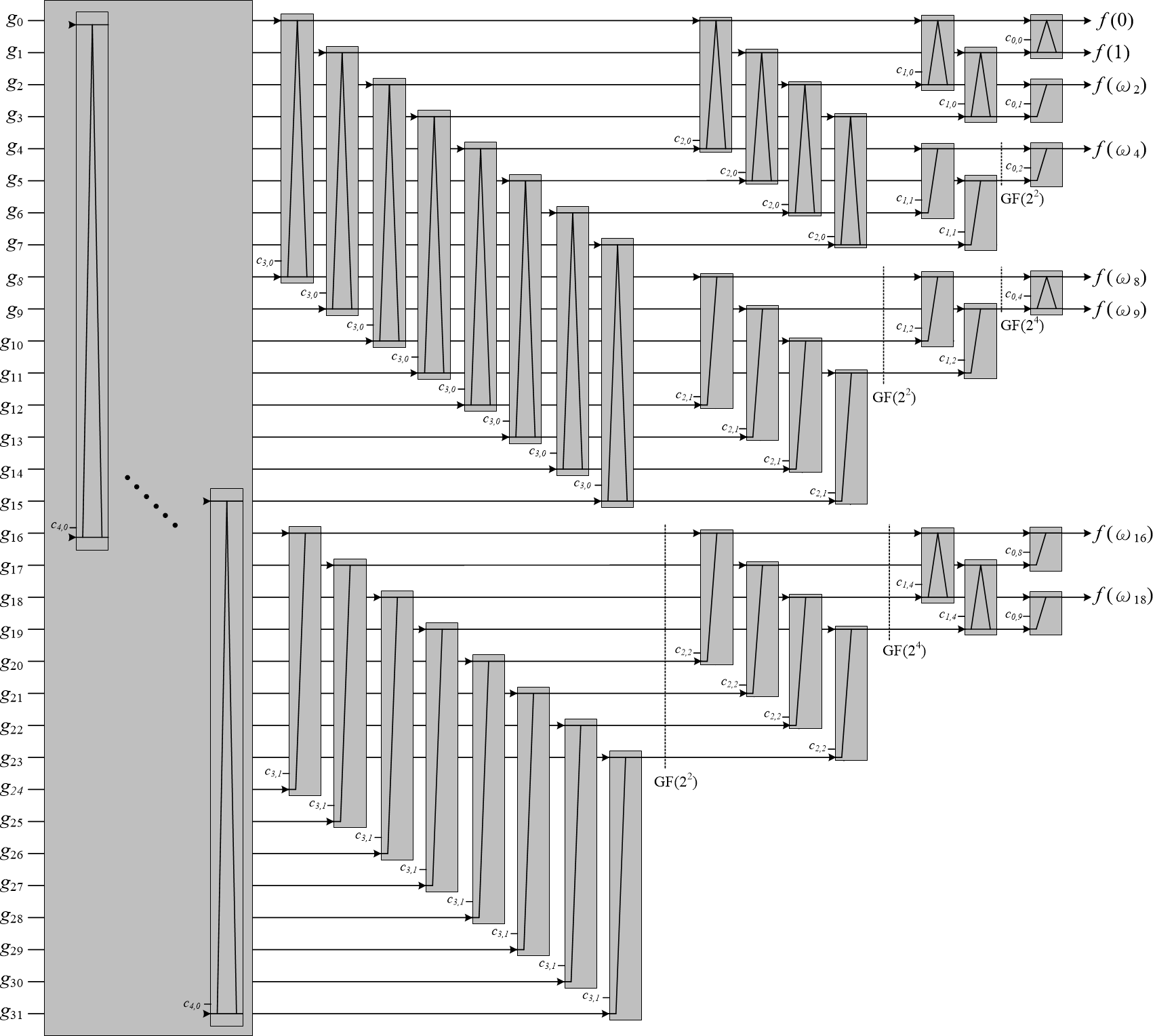
Figure 1. Illustration of the butterfly network with $n=32$. $f(0),f(1)\in\mathbb{F}_{2},f(\omega_{2})\in\mathbb{F}_{2^{2}},f(\omega_{4}),f(\omega_{8}),f(\omega_{9})\in\mathbb{F}_{2^{4}}$ and $f(\omega_{16}),f(\omega_{18})\in\mathbb{F}_{2^{8}}$

3.4. Complexity Analysis

In this section, we analyze the complexity of FAFFT in algorithm 3. Let $F(k,l)$ and $F_{A}(k,l)$ denote the cost of multiplication and addition to compute $\texttt{FAFFT}(k,P(x),l,\alpha)$ for $P(x)\in\mathbb{F}_{2}[x]_{<2^{k}}$ and $\alpha\in W_{k+l}\setminus W_{k}$.

First, it is straightforward to verify that for all $\texttt{FAFFT}(k^{\prime},P^{\prime}(x),l^{\prime},\alpha^{\prime})$ call during recursion:

• $\alpha^{\prime}\in W_{k^{\prime}+l^{\prime}}\setminus W_{k^{\prime}}$ if $l^{\prime}>0$ , otherwise $\alpha^{\prime}=0$

• $P^{\prime}(x)=\sum p^{\prime}_{i}X_{i}(x)$, $p^{\prime}_{i}\in\mathbb{F}_{2^{2^{\lceil\lg{l^{\prime}}\rceil}}}$ if $l^{\prime}>0$, $p^{\prime}_{i}\in\mathbb{F}_{2}$ otherwise.

• $\!\begin{aligned} s_{k-1}(\alpha^{\prime})&\in(W_{l^{\prime}+1}\setminus W_{l^{\prime}})\\ &\in\begin{cases}u_{\lg{l^{\prime}}}+\mathbb{F}_{l^{\prime}}&\text{if }l^{\prime}\text{ is a power of two}\\ \mathbb{F}_{2^{\lceil\lg{l^{\prime}}\rceil}}&\text{ otherwise}\end{cases}\end{aligned}$

Then we have

$$F(k,l)=\begin{cases}F(k-1,l)+F(k-1,l+1)+2^{k-1}(M(1))&\text{if }l=0\\ F(k-1,l+1)+2^{k-1}(M(l))&\text{if }l\text{ is a power of two}\\ 2\cdot F(k-1,l+1)+2^{k-1}(M(2^{\lceil\lg{l}\rceil}))&\text{otherwise}\end{cases}$$

Theorem 3.4.

(multiplication complexity) Given $n=2^{m}$, for $m+l\leq d$, d is a power of two. Then we have

$$F(m,l)\leq\begin{cases}\frac{1}{2}(n\lg n\frac{M(d)}{d})&\text{if }l=0\\ \frac{1}{2}(n\lg n\frac{M(d)}{d}2^{\lceil\lg{l}\rceil})&\text{otherwise}\\ \end{cases}$$

Proof.

We prove by induction. Consider $m=1$, then $F(1,l)=M(l)\leq\frac{M(d)}{d}l$ is correct.

Assume $m=k-1$ and for any $l\leq d-m$,

$$F(m,l)\leq\begin{cases}\frac{1}{2}m2^{m}\frac{M(d)}{d}&\text{if }l=0\\ \frac{1}{2}m2^{m}\frac{M(d)}{d}2^{\lceil\lg{l}\rceil}&\text{otherwise}\\ \end{cases}$$

Then we check three cases: first, $m=k$ and $l=0$:

$$F(k,l) =F(k-1,0)+F(k-1,1)+2^{k-1}\cdot M(1)$$

$$=\frac{1}{2}(k-1)2^{k}\frac{M(d)}{d}+2^{k}\cdot M(1)$$

$$\leq\frac{1}{2}k2^{k}\frac{M(d)}{d}$$

Second, $m=k$ and $l$ is a power of two:

$$F(k,l) =F(k-1,l+1)+\cdot 2^{k-1}\cdot M(l)$$

$$=(k-1)2^{k}\frac{M(d)}{d}l+2^{k-1}\cdot M(l)$$

$$\leq\frac{1}{2}(k-1)2^{k}\frac{M(d)}{d}l+2^{k-1}\frac{M(d)}{d}l$$

$$=\frac{1}{2}k2^{k}\frac{M(d)}{d}l$$

Finally, $l>0$ and is not a power of two:

$$F(k,l) =2\cdot F(k-1,l+1)+2^{k-1}\cdot M(2^{\lceil\lg{l}\rceil})$$

$$=\frac{1}{2}(k-1)2^{k}\frac{M(d)}{d}2^{\lceil\lg{l+1}\rceil}+2^{k-1}\cdot M(2^{\lceil\lg{l}\rceil})$$

$$\leq\frac{1}{2}(k-1)2^{k}\frac{M(d)}{d}2^{\lceil\lg{l}\rceil}+2^{k-1}\cdot\frac{M(2^{\lceil\lg{l}\rceil})}{2^{\lceil\lg{l}\rceil}}2^{\lceil\lg{l}\rceil}$$

$$\leq\frac{1}{2}k2^{k}\frac{M(d)}{d}l$$

Note that we assume $\frac{M(l)}{l}$ is increasing in $l$. We complete the proof.

∎

For the cost of addition, it can be proved follow the same procedure above since each with $2A(d)$ instead of $M(d)$. (Note that $\frac{A(d)}{d}$ is constant)

Theorem 3.5.

(addition complexity) Given $n=2^{m}$, for $m+l\leq d$, d is a power of two. Then we have

$$F_{A}(m,l)\leq\begin{cases}(n\lg n\frac{A(d)}{d})&\text{if }l=0\\ (n\lg n\frac{A(d)}{d}2^{\lceil\lg{l}\rceil})&\text{otherwise}\\ \end{cases}$$

Given $P\in\mathbb{F}_{2}[x]_{<n}$ and $n$ a power of two, to compute $\textit{FAFT}_{n}(P)$, we call $\texttt{FAFFT}(\lg(n),P,0,0)$. Thus, the cost of compute $\textit{FAFT}_{n}(P)$ is $\frac{1}{2}n\lg{(n)}\frac{M(d)}{d}+n\lg{(n)}\frac{A(d)}{d}$. Compare with the additive FFT for $\mathbb{F}_{2^{d}}[x]_{<n}$ whose cost is $\frac{1}{2}(n\lg(n)(M(d)+2A(d))$, we gain a speed-up factor $d$.

3.5. Inverse Frobenius additive FFT

The inverse Frobenius additive FFT is straight forward because for the butterfly unit with two output, it is easy to find its inverse.

However, due to the truncation, it is not obvious how to inverse when $l$ is a power of two. Here we show that it is always invertible. In the algorithm 3, when $l$ is a power of two, it truncates and only compute FAFT  of $Q_{0}(x)=P_{0}(x)+s_{k-1}(\alpha)\cdot P_{1}(x)$. To be able to inverse, we need to recover $P_{0}(x)$ and $P_{1}(x)$ from $Q_{0}(x)$. Note that $s_{k-1}(\alpha)\in(W_{l+1}\setminus W_{l})=v_{l}+W_{l}$ because $\alpha\in W_{k+l+1}\in W_{k+l}$ and lemma 2.7. Since we use Cantor basis, recall the definition 2.1, $v_{l}=u_{\lg{l}}$ when $l$ is a power of two. We can rewrite the equation from the point of $\mathbb{F}_{2^{l}}[u_{\lg{l}}][x]$. Let $s_{k-1}(\alpha)=u_{\lg l}+c$ and $c\in\mathbb{F}_{2^{l}}$,

$$Q_{0}(x)=R_{0}(x)+R_{1}(x)u_{\lg l}=P_{0}(x)+(c+u_{\lg l})\cdot P_{1}(x)$$

where $R_{0}(x),R_{1}(x)\in\mathbb{F}_{2^{l}}[x]$. Then we get

$$P_{0}(x) =R_{0}(x)+R_{1}(x)\cdot c$$

$$P_{1}(x) =R_{1}(x)$$

Thus we can always recover $P_{0}(x)$ and $P_{1}(x)$ from $Q(x)$. The full inverse Frobenius additive FFT algorithm is shown in algorithm 4.

IFAFFT($k,A,l,\alpha$) :

input : $A=P(\sigma)_{\sigma\in\Sigma}$ where $\Sigma=(\Sigma_{0}\cup\Sigma_{1}\cup\ldots\cup\Sigma_{k+l})\cap(\alpha+W_{k})$,

$\alpha\in W_{k+l}\setminus W_{k}$ if $l>0$ , otherwise $\alpha=0$.

output :  $P(x)=p_{0}X_{0}(x)+p_{1}X_{1}(x)+...+p_{2^{k}-1}X_{2^{k}-1}(x)$ : $p_{i}\in\mathbb{F}_{2^{2^{\lceil\lg{l}\rceil}}}$ if $l>0$, $p_{i}\in\mathbb{F}_{2}$ otherwise.

if  $k=0$  then  return the only element in $A$ ;

if $l=0$ then

       Divide the set $A$ to $A_{0}$, $A_{1}$

       $Q_{0}(x)\leftarrow$ IFAFFT($k-1,A_{0},l,\alpha$)

       $Q_{1}(x)\leftarrow$ IFAFFT($k-1,A_{1},l+1,v_{k-1}+\alpha$)

       $P_{1}(x)\leftarrow(Q_{0}(x)+Q_{1}(x))$

      $P_{0}(x)\leftarrow Q_{0}(x)+s_{k-1}(\alpha)\cdot P_{1}(x)$

      

else if $l=2^{\lfloor\lg{(l)}\rfloor}$ then

       $Q(x)\leftarrow$IFAFFT($k-1,A,l+1,\alpha$)

       Let $s_{k-1}(\alpha)=c+u_{\lg(l)}$

       Let $Q(x)=R_{0}(x)+u_{\lg(l)}\cdot R_{1}(x)$

       $P_{0}(x)\leftarrow R_{0}(x)+R_{1}(x)\cdot c$

       $P_{1}(x)\leftarrow R_{1}(x)$

      

else

       Divide the set $A$ to $A_{0}$, $A_{1}$

       $Q_{0}(x)\leftarrow$ IFAFFT($k-1,A_{0},l+1,\alpha$)

       $Q_{1}(x)\leftarrow$ IFAFFT($k-1,A_{1},l+1,v_{k-1}+\alpha$)

       $P_{1}(x)\leftarrow Q_{0}(x)+Q_{1}(x)$

       $P_{0}(x)\leftarrow Q_{0}(x)+s_{k-1}(\alpha)\cdot P_{1}(x)$

      

end if

return $P_{0}(x)+P_{1}(x)\cdot s_{k-1}(x)$

Algorithm 4 Inverse Frobenius Additive FFT in novel polynomial basis.

4. Multiplications in $\mathbb{F}_{2}[x]$

To multiply a polynomial using Frobenius additive FFT is exactly the same as conventional way: applying basis conversion to convert to novel polynomial basis, computing Frobenius additive FFT, pair-wise multiplication, computing the inverse Frobenius additive FFT, then transforming back into the original monomial basis.

4.1. Multiplications of $\mathbb{F}_{2}[x]$ of small degree

The record of minimal bit-operation to multiply polynomial over $\mathbb{F}_{2}[x]$ was set by (Ber, 09) and (CH, 15), which are both based on Karatsuba-like algorithm. Instead of Karatsuba-like algorithm, we use Frobenius additive FFT to perform multiplication in $\mathbb{F}_{2}[x]$. We implement a generator to generate code of binary polynomial multiplication with size $2^{m}$ where each variable is in $\mathbb{F}_{2}$. Since the multiplicands $s_{k}(\alpha)$ in FAFFT can all be precomputed. To reduce the number of bit operations, when multiplying a constant, we transform it into a matrix vector product over $\mathbb{F}_{2}$ and apply common subexpression algorithm as in (Paa, 97). The generated code consists of XOR and AND expressions. The generator will be made public available on Github.

In figure 2, we show the best results of polynomial multiplication over binary field. (Ber, 09) set the record for polynomial size up to 1000 in 2009. (CH, 15) improve the results up to 4.5% for certain size of polynomial. Since our Frobenius Additive FFT works with the polynomial size equal to power of two, we apply it to polynomial multiplication with polynomial size 256, 512, and 1024. We improve the best known results by 19.1%, 29.7%, and 41.1% respectively. To conclude the comparison, we set the record of size 231 to 256, 414 to 512, and 709 to 1024 just by above result. To the best of our knowledge, it is the first time FFT-based method outperforms Karatsuba-like algorithm in such low degree in terms of bit operation count. In addition, for polynomial size 128, our FAFFT costs 11556 bit operations, comparing to the best previous is 11466 from (CH, 15). Our result is only 0.78% slight slower in terms of bit operation count.

Figure 2. Number of bit operations for multiplication of $\mathbb{F}_{2}[x]$

4.1.1. Other FFT-based multiplication using Kronecker method

In (BC, 14), an optimized implementation of additive FFT based on (GM, 10) was presented. They show the cost of multiplication in $\mathbb{F}_{2^{8}}[x]_{<32}$ is 22,292 bit operations. We can use it to multiply polynomials of degree $128$ using Kronecker method. But our Frobenius additive FFT only requires 11556 for size 128, which is about half of their results. The factor $2$ speedup compared with Kronecker method is expected as in (vdHL17a, ) because the total bit length is half when using Frobenius method.

4.1.2. Application to Binary Elliptic Curve Cryptography

There are several polynomial sizes that are in the interest of cryptography engineering community and its number of bit operation of multiplication were studied due to its application in binary elliptic curve(Ber, 09) (CH, 15). These binary elliptic curve includes: Koblitz curve sect233k1, sect233r1 over $\mathbb{F}_{2}[x]/(x^{233}+x^{74}+1)$, curve sect239k1, sect239r1 over $\mathbb{F}_{2}[x]/(x^{239}+x^{158}+1)$, and Edwards curve BBE251 over $\mathbb{F}_{2}[x]/(x^{251}+x^{7}+x^{4}+x^{2}+1)$ according to Standards for Efficient Cryptography Group (SECG) and (Ber, 09). For the corresponding polynomial size $233$, $239$ and $251$, the Frobenius additive FFT method outperforms previous method in terms of number of bit operations. Thus, our FAFFT can potentially applied to these curve in order to accelerate the computation.

4.2. Multiplication of $\mathbb{F}_{2}[x]$ of large degree

Another application is to implement multiplications of $\mathbb{F}_{2}[x]$ of large degree on modern CPU. Here we will implement a variant of the algorithm. The bit operation count is not a good predictor on modern CPU since they operate on 64-bit machine words and there are special instruction PCLMULQDQ designed for carryless multiplication with input size $64$. As in (VDHLL, 17), to implement on modern CPU, we have to take these into account. To be able to use PCLMULQDQ, we change our algorithm to only compute a subset of cross section. The set of point we will use is

$$\{v_{i-1}+v_{i-2}j_{1}+v_{i-3}j_{2}+\ldots+v_{0}j_{i-1}: j_{k}=0\text{ if }k\leq 64,$$

$$j_{k}\in\{0,1\}\text{ otherwise}\}$$

where $64<i\leq 128$. By selecting this subset, we can mostly operate in $\mathbb{F}_{2^{128}}$ and mainly use the PCLMULQDQ instruction which performs carryless multiplication with input size 64. We show the benchmark on Intel Skylake architecture in Table 1 with comparison of other implementations. In the table, for polynomial of size $n$ where $\log_{2}(n/64)=16,17,\ldots,23$, our implementation of variant of FAFFT outperforms previous best results from (VDHLL, 17; CCK⁺, 17; HvdHL, 16; BGTZ, 08).

Table 1. Products in degree $<n$ in $\mathbb{F}_{2}[x]$ on Intel Skylake Xeon E3-1275 v5 @ 3.60GHz ($10^{-3}$ sec.)

$\log_{2}(n/64)$	16	17	18	19	20	21	22	23
This work, $\mathbb{F}_{2^{128}}$	9	20	41	88	192	418	889	1865
FDFT (VDHLL, 17) c	11	24	56	127	239	574	958	2465
ADFT(CCK+, 17)	16	34	74	175	382	817	1734	3666
$\mathbb{F}_{2^{60}}$(HvdHL, 16)b	22	51	116	217	533	885	2286	5301
gf2x a (BGTZ, 08)	23	51	111	250	507	1182	2614	6195

• Version 1.2. Available from http://gf2x.gforge.inria.fr/

• SVN r10663. Available from svn://scm.gforge.inria.fr/svn/mmx

• SVN r10681. Available from svn://scm.gforge.inria.fr/svn/mmx

5. Future Direction

This is the first time FFT-based algorithm that outperforms Karatsuba-like algorithm for binary polynomial multiplication in such low degree. We hope our work can open up a new direction for the community interested in the number bit operation of binary polynomial multiplication in small degree, as there are possible future work such as further reducing bit operations in (BC, 14) or using truncated method to eliminate the ‘jump‘ in the complexity when size is a power of two (vdH, 04).

References

- BC [14] Daniel J. Bernstein and Tung Chou. Faster binary-field multiplication and faster binary-field macs. In Antoine Joux and Amr M. Youssef, editors, Selected Areas in Cryptography - SAC 2014 - 21st International Conference, Montreal, QC, Canada, August 14-15, 2014, Revised Selected Papers, volume 8781 of Lecture Notes in Computer Science, pages 92–111. Springer, 2014.
- Ber [09] Daniel J. Bernstein. Batch binary edwards. In Advances in Cryptology - CRYPTO 2009, 29th Annual International Cryptology Conference, Santa Barbara, CA, USA, August 16-20, 2009. Proceedings, pages 317–336, 2009.
- BGTZ [08] Richard P Brent, Pierrick Gaudry, Emmanuel Thomé, and Paul Zimmermann. Faster multiplication in gf (2)(x). Lecture Notes in Computer Science, 5011:153–166, 2008.
- BYD [17] Michael A. Burr, Chee K. Yap, and Mohab Safey El Din, editors. Proceedings of the 2017 ACM on International Symposium on Symbolic and Algebraic Computation, ISSAC 2017, Kaiserslautern, Germany, July 25-28, 2017. ACM, 2017.
- Can [89] David G. Cantor. On arithmetical algorithms over finite fields. J. Comb. Theory Ser. A, 50(2):285–300, March 1989.
- CCK+ [17] Ming-Shing Chen, Chen-Mou Cheng, Po-Chun Kuo, Wen-Ding Li, and Bo-Yin Yang. Faster multiplication for long binary polynomials. CoRR, abs/1708.09746, 2017.
- CH [15] Murat Cenk and M. Anwar Hasan. Some new results on binary polynomial multiplication. J. Cryptographic Engineering, 5(4):289–303, 2015.
- CHN [14] Murat Cenk, M. Anwar Hasan, and Christophe Nègre. Efficient subquadratic space complexity binary polynomial multipliers based on block recombination. IEEE Trans. Computers, 63(9):2273–2287, 2014.
- CNH [13] Murat Cenk, Christophe Nègre, and M. Anwar Hasan. Improved three-way split formulas for binary polynomial and toeplitz matrix vector products. IEEE Trans. Computers, 62(7):1345–1361, 2013.
- FH [15] Haining Fan and M. Anwar Hasan. A survey of some recent bit-parallel gf ( 2 n ) multipliers. Finite Fields Appl., 32(C):5–43, March 2015.
- GM [10] Shuhong Gao and Todd Mateer. Additive fast fourier transforms over finite fields. IEEE Trans. Inf. Theor., 56(12):6265–6272, December 2010.
- HvdHL [16] David Harvey, Joris van der Hoeven, and Grégoire Lecerf. Fast polynomial multiplication over . In Sergei A. Abramov, Eugene V. Zima, and Xiao-Shan Gao, editors, Proceedings of the ACM on International Symposium on Symbolic and Algebraic Computation, ISSAC 2016, Waterloo, ON, Canada, July 19-22, 2016, pages 255–262. ACM, 2016.
- HvdHL [17] David Harvey, Joris van der Hoeven, and Grégoire Lecerf. Faster polynomial multiplication over finite fields. J. ACM, 63(6):52:1–52:23, 2017.
- JKR [12] Charanjit S. Jutla, Vijay Kumar, and Atri Rudra. On the circuit complexity of composite galois field transformations. Electronic Colloquium on Computational Complexity (ECCC), 19:93, 2012.
- LANH [16] Sian-Jheng Lin, Tareq Y. Al-Naffouri, and Yunghsiang S. Han. Fft algorithm for binary extension finite fields and its application to reed–solomon codes. IEEE Trans. Inf. Theor., 62(10):5343–5358, October 2016.
- LCH [14] Sian-Jheng Lin, Wei-Ho Chung, and Yunghsiang S. Han. Novel polynomial basis and its application to reed-solomon erasure codes. In 55th IEEE Annual Symposium on Foundations of Computer Science, FOCS 2014, Philadelphia, PA, USA, October 18-21, 2014, pages 316–325. IEEE Computer Society, 2014.
- Paa [97] C. Paar. Optimized arithmetic for reed-solomon encoders. In Proceedings of IEEE International Symposium on Information Theory, pages 250–, Jun 1997.
- vdH [04] Joris van der Hoeven. The truncated fourier transform and applications. In Jaime Gutierrez, editor, Symbolic and Algebraic Computation, International Symposium ISSAC 2004, Santander, Spain, July 4-7, 2004, Proceedings, pages 290–296. ACM, 2004.
- [19] Joris van der Hoeven and Robin Larrieu. The frobenius FFT. In Burr et al. [4], pages 437–444.
- [20] Joris van der Hoeven and Grégoire Lecerf. Composition modulo powers of polynomials. In Burr et al. [4], pages 445–452.
- VDHLL [17] Joris Van Der Hoeven, Robin Larrieu, and Grégoire Lecerf. Implementing fast carryless multiplication. working paper or preprint, August 2017.
- vzGS [05] Joachim von zur Gathen and Jamshid Shokrollahi. Efficient fpga-based karatsuba multipliers for polynomials over f. In Bart Preneel and Stafford E. Tavares, editors, Selected Areas in Cryptography, 12th International Workshop, SAC 2005, Kingston, ON, Canada, August 11-12, 2005, Revised Selected Papers, volume 3897 of Lecture Notes in Computer Science, pages 359–369. Springer, 2005.