Detecting and Correcting for Label Shift with Black Box Predictors

Abstract

Faced with distribution shift between training and test set, we wish to detect and quantify the shift, and to correct our classifiers without test set labels. Motivated by medical diagnosis, where diseases (targets), cause symptoms (observations), we focus on label shift, where the label marginal $p(y)$ changes but the conditional $p(\boldsymbol{x}|y)$ does not. We propose Black Box Shift Estimation (BBSE) to estimate the test distribution $p(y)$. BBSE exploits arbitrary black box predictors to reduce dimensionality prior to shift correction. While better predictors give tighter estimates, BBSE works even when predictors are biased, inaccurate, or uncalibrated, so long as their confusion matrices are invertible. We prove BBSE’s consistency, bound its error, and introduce a statistical test that uses BBSE to detect shift. We also leverage BBSE to correct classifiers. Experiments demonstrate accurate estimates and improved prediction, even on high-dimensional datasets of natural images.

1 Introduction

Assume that in August we train a pneumonia predictor. Our features consist of chest X-rays administered in the previous year (distribution $P$) and the labels binary indicators of whether a physician diagnoses the patient with pneumonia. We train a model $f$ to predict pneumonia given an X-ray image. Assume that in the training set $.1\%$ of patients have pneumonia. We deploy $f$ in the clinic and for several months, it reliably predicts roughly $.1\%$ positive.

Fast-forward to January (distribution $Q$): Running $f$ on the last week’s data, we find that $5\%$ of patients are predicted to have pneumonia! Because $f$ remains fixed, the shift must owe to a change in the marginal $p(\boldsymbol{x})$, violating the familiar iid assumption. Absent familiar guarantees, we wonder: Is $f$ still accurate? What’s the real current rate of pneumonia? Shouldn’t our classifier, trained under an obsolete prior, underestimate pneumonia when uncertain? Thus, we might suspect that the real prevalence is greater than $5\%$.

Given only labeled training data, and unlabeled test data, we desire to: (i) detect distribution shift, (ii) quantify it, and (iii) correct our model to perform well on the new data. Absent assumptions on how $p(y,\boldsymbol{x})$ changes, the task is impossible. However, under assumptions about what P and Q have in common, we can still make headway. Two candidates are covariate shift (where $p(y|\boldsymbol{x})$ does not change) and label shift (where $p(\boldsymbol{x}|y)$ does not change). Schölkopf et al. (2012) observe that covariate shift corresponds to causal learning (predicting effects), and label shift to anticausal learning (predicting causes).

We focus on label shift, motivated by diagnosis (diseases cause symptoms) and recognition tasks (objects cause sensory observations). During a pneumonia outbreak, $p(y|\boldsymbol{x})$ (e.g. flu given cough) might rise but the manifestations of the disease $p(\boldsymbol{x}|y)$ might not change. Formally, under label shift, we can factorize the target distribution as

$$q(y,\boldsymbol{x})=q(y)p(\boldsymbol{x}|y).$$

By contrast, under the covariate shift assumption, $q(y,\boldsymbol{x})=q(\boldsymbol{x})p(y|\boldsymbol{x})$, e.g. the distribution of radiologic findings $p(\boldsymbol{x})$ changes, but the conditional probability of pneumonia $p(y|\boldsymbol{x})$ remains constant. To see how this can go wrong, consider: what if our only feature were cough? Normally, cough may not (strongly) indicate pneumonia. But during an epidemic, $\mathbb{P}(\text{pneumonia}|\text{cough})$ might go up substantially. Despite its importance, label shift is comparatively under-investigated, perhaps because given samples from both $p(\boldsymbol{x})$ and $q(\boldsymbol{x})$, quantifying $q(\boldsymbol{x})/p(\boldsymbol{x})$ is more intuitive.

We introduce Black Box Shift Estimation (BBSE) to estimate label shift using a black box predictor $f$. BBSE estimates the ratios $w_{l}=q(y_{l})/p(y_{l})$ for each label $l$, requiring only that the expected confusion matrix is invertible . We estimate $\hat{\boldsymbol{w}}$ by solving a linear system $A\boldsymbol{x}=b$ where $A$ is the confusion matrix of $f$ estimated on training data (from P) and $b$ is the average output of $f$ calculated on test samples (from Q). We make the following contributions:

1. Consistency and error bounds for BBSE.

2. Applications of BBSE to statistical tests for detecting distribution label shift

3. Model correction through importance-weighted Empirical Risk Minimization.

4. A comprehensive empirical validation of BBSE.

Compared to approaches based on Kernel Mean Matching (KMM) (Zhang et al., 2013), EM (Chan & Ng, 2005), and Bayesian inference (Storkey, 2009), BBSE offers the following advantages: (i) Accuracy does not depend on data dimensionality; (ii) Works with arbitrary black box predictors, even biased, uncalibrated, or inaccurate models; (iii) Exploits advances in deep learning while retaining theoretical guarantees: better predictors provably lower sample complexity; and (iv) Due to generality, could be a standard diagnostic / corrective tool for arbitrary ML models.

2 Prior Work

Despite its wide applicability, learning under label shift with unknown $q(y)$ remains curiously under-explored. Noting the difficulty of the problem, Storkey (2009) proposes placing a (meta-)prior over $p(y)$ and inferring the posterior distribution from unlabeled test data. Their approach requires explicitly estimating $p(\boldsymbol{x}|y)$, which may not be feasible in high-dimensional datasets. Chan & Ng (2005) infer $q(y)$ using EM but their method also requires estimating $p(\boldsymbol{x}|y)$. Schölkopf et al. (2012) articulates connections between label shift and anti-causal learning and Zhang et al. (2013) extend the kernel mean matching approach due to (Gretton et al., 2009) to the label shift problem. When $q(y)$ is known, label shift simplifies to the problem of changing base rates (Bishop, 1995; Elkan, 2001). Previous methods require estimating $q(\boldsymbol{x})$, $q(\boldsymbol{x})/p(\boldsymbol{x})$, or $p(\boldsymbol{x}|y)$, often relying on kernel methods, which scale poorly with dataset size and underperform on high-dimensional data.

Covariate shift, also called sample selection bias, is well-studied (Zadrozny, 2004; Huang et al., 2007; Sugiyama et al., 2008; Gretton et al., 2009). Shimodaira (2000) proposed correcting models via weighting examples in ERM by $q(\boldsymbol{x})/p(\boldsymbol{x})$. Later works estimate importance weights from the available data, e.g., Gretton et al. (2009) propose kernel mean matching to re-weight training points.

The earliest relevant work to ours comes from econometrics and addresses the use of non-random samples to estimate behavior. Heckman (1977) addresses sample selection bias, while (Manski & Lerman, 1977) investigates estimating parameters under choice-based and endogenous stratified sampling, cases analogous to a shift in the label distribution. Also related, Rosenbaum & Rubin (1983) introduce propensity scoring to design unbiased experiments. Finally, we note a connection to cognitive science work showing that humans classify items differently depending on other items they appear alongside (Zhu et al., 2010).

Post-submission, we learned of antecedents for our estimator in epidemiology (Buck et al., 1966) and revisited by Forman (2008); Saerens et al. (2002). These papers do not develop our theoretical guarantees or explore the modern ML setting where $\boldsymbol{x}$ is massively higher-dimensional than $y$, bolstering the value of dimensionality reduction.

3 Problem setup

We use $\boldsymbol{x}\in\mathcal{X}=\mathbb{R}^{d}$ and $y\in\mathcal{Y}$ to denote the feature and label variables. For simplicity, we assume that $\mathcal{Y}$ is a discrete domain equivalent to $\{1,2,...,k\}$. Let $P,Q$ be the source and target distributions defined on $\mathcal{X}\times\mathcal{Y}$. We use $p,q$ to denote the probability density function (pdf) or probability mass function (pmf) associated with $P$ and $Q$ respectively. The random variable of interest is clear from context. For example, $p(y)$ is the p.m.f. of $y\sim P$ and $q(\boldsymbol{x})$ is the p.d.f. of $\boldsymbol{x}\sim Q$. Moreover, $p(y=i)$ and $q(y=i)$ are short for $\mathbb{P}_{P}(y=i)$ and $\mathbb{P}_{Q}(y=i)$ respectively, where $\mathbb{P}(S):=\mathbb{E}[\mathbf{1}(S)]$ denotes the probability of an event $S$ and $\mathbb{E}[\cdot]$ denotes the expectation. Subscripts $P$ and $Q$ on these operators make the referenced distribution clear.

In standard supervised learning, the learner observes training data $(\boldsymbol{x}_{1},y_{1}),(\boldsymbol{x}_{2},y_{2}),...,(\boldsymbol{x}_{n},y_{n})$ drawn iid from a training (or source) distribution $P$. We denote the collection of feature vectors by $X\in\mathbb{R}^{n\times d}$ and the label by $\boldsymbol{y}$. Under Domain Adaptation (DA), the learner additionally observes a collection of samples $X^{\prime}=[\boldsymbol{x}^{\prime}_{1};...;\boldsymbol{x}^{\prime}_{m}]$ drawn iid from a test (or target) distribution $Q$. Our objective in DA is to predict well for samples drawn from $Q$.

In general, this task is impossible – $P$ and $Q$ might not share support. This paper considers $3$ extra assumptions:

The label shift (also known as target shift) assumption

$$p(\boldsymbol{x}|y)=q(\boldsymbol{x}|y)\quad\forall\;x\in\mathcal{X},\;y\in\mathcal{Y}.$$

For every $y\in\mathcal{Y}$ with $q(y)>0$ we require $p(y)>0$.

Access to a black box predictor $f:\mathcal{X}\rightarrow\mathcal{Y}$ where the expected confusion matrix $\mathbf{C}_{p}(f)$ is invertible.

$$\mathbf{C}_{P}(f):=p(f(\boldsymbol{x}),y)\in\mathbb{R}^{|\mathcal{Y}|\times|\mathcal{Y}|}$$

We now comment on the assumptions. A.1 corresponds to anti-causal learning. This assumption is strong but reasonable in many practical situations, including medical diagnosis, where diseases cause symptoms. It also applies when classifiers are trained on non-representative class distributions: Note that while visions systems are commonly trained with balanced classes (Deng et al., 2009), the true class distribution for real tasks is rarely uniform.

Assumption A.2 addresses identifiability, requiring that the target label distribution’s support be a subset of training distribution’s. For discrete $\mathcal{Y}$, this simply means that the training data should contain examples from every class.

Assumption A.3 requires that the expected predictor outputs for each class be linearly independent. This assumption holds in the typical case where the classifier predicts class $y_{i}$ more often given images actually belong to $y_{i}$ than given images from any other class $y_{j}$. In practice, $f$ could be a neural network, a boosted decision-tree or any other classifier trained on a holdout training data set. We can verify at training time that the empirical estimated normalized confusion matrix is invertible. Assumption A.3 generalizes naturally to soft-classifiers, where $f$ outputs a probability distribution supported on $\mathcal{Y}$. Thus BBSE can be applied even when the confusion matrix is degenerate.

We wish to estimate $w(y):=q(y)/p(y)$ for every $y\in\mathcal{Y}$ with training data, unlabeled test data and a predictor $f$. This estimate enables DA techniques under the importance-weighted ERM framework, which solves $\min\sum_{i=1}^{n}w_{i}\ell(y_{i},\boldsymbol{x}_{i})$, using $w_{i}=q(\boldsymbol{x}_{i},y_{i})/p(\boldsymbol{x}_{i},y_{i})$. Under the label shift assumption, the importance weight $w_{i}=q(y_{i})/p(y_{i})$. This task isn’t straightforward because we don’t observe samples from $q(y)$.

4 Main results

We now derive the main results for estimating $w(y)$ and $q(y)$. Assumption A.1 has the following implication:

Lemma 1.

Denote by $\hat{y}=f(\boldsymbol{x})$ the output of a fixed function $f:\mathcal{X}\rightarrow\mathcal{Y}$. If Assumption A.1 holds, then

$$q(\hat{y}|y)=p(\hat{y}|y).$$

The proof is simple: recall that $\hat{y}$ depends on $y$ only via $\boldsymbol{x}$. By A.1, $p(\boldsymbol{x}|y)=q(\boldsymbol{x}|y)$ and thus $q(\hat{y}|y)=p(\hat{y}|y)$.

Next, combine the law of total probability and Lemma 1 and we arrive at

$$q(\hat{y})= \sum_{y\in\mathcal{Y}}q(\hat{y}|y)q(y)$$

$$= \sum_{y\in\mathcal{Y}}p(\hat{y}|y)q(y)=\sum_{y\in\mathcal{Y}}p(\hat{y},y)\frac{q(y)}{p(y)}.$$ (1)

We estimate $p(\hat{y}|y)$ and $p(\hat{y},y)$ using $f$ and data from source distribution $P$, and $q(\hat{y})$ with unlabeled test data drawn from target distribution $Q$. This leads to a novel method-of-moments approach for consistent estimation of the shifted label distribution $q(y)$ and the weights $w(y)$.

Without loss of generality, we assume $\mathcal{Y}=\{1,2,...,k\}$. Denote by $\boldsymbol{\nu}_{y},\boldsymbol{\nu}_{\hat{y}},\hat{\boldsymbol{\nu}}_{\hat{y}},\boldsymbol{\mu}_{y},\boldsymbol{\mu}_{\hat{y}},\hat{\boldsymbol{\mu}}_{\hat{y}},\boldsymbol{w}\in\mathbb{R}^{k}$ moments of $p$, $q$, and their plug-in estimates, defined via

$$[\boldsymbol{\nu}_{y}]_{i} =p(y=i) [\boldsymbol{\mu}_{y}]_{i} =q(y=i)$$

$$[\boldsymbol{\nu}_{\hat{y}}]_{i} =p(f(\boldsymbol{x})=i) [\boldsymbol{\mu}_{\hat{y}}]_{i} =q(f(\boldsymbol{x})=i)$$

$$[\hat{\boldsymbol{\nu}}_{\hat{y}}]_{i} =\frac{\sum_{j}\mathbbm{1}\{f(\boldsymbol{x}_{j})=i\}}{n} [\hat{\boldsymbol{\mu}}_{\hat{y}}]_{i} =\frac{\sum_{j}\mathbbm{1}\{f(\boldsymbol{x}_{j}^{\prime})=i\}}{m}$$

and $[\boldsymbol{w}]_{i}=q(y=i)/p(y=i)$. Lastly define the covariance matrices $\mathbf{C}_{\hat{y},y},\mathbf{C}_{\hat{y}|y}$ and $\hat{\mathbf{C}}_{\hat{y},y}$ in $\mathbb{R}^{k\times k}$ via

$$[\mathbf{C}_{\hat{y},y}]_{ij} =p(f(\boldsymbol{x})=i,y=j)$$

$$[\mathbf{C}_{\hat{y}|y}]_{ij} =p(f(\boldsymbol{x})=i|y=j)$$

$$[\hat{\mathbf{C}}_{\hat{y},y}]_{ij} =\frac{1}{n}\sum_{l}\mathbbm{1}\{f(\boldsymbol{x}_{l})=i\text{ and }y_{l}=j\}$$

We can now rewrite Equation (1) in matrix form:

$$\boldsymbol{\mu}_{\hat{y}}={\mathbf{C}}_{\hat{y}|y}\boldsymbol{\mu}_{y}=\mathbf{C}_{\hat{y},y}\boldsymbol{w}$$

Using plug-in maximum likelihood estimates of the above quantities yields the estimators

$$\hat{\boldsymbol{w}}=\hat{\mathbf{C}}_{\hat{y},y}^{-1}\hat{\boldsymbol{\mu}}_{\hat{y}}\text{ and }\hat{\boldsymbol{\mu}}_{y}=\mathrm{diag}(\hat{\boldsymbol{\nu}}_{y})\hat{\boldsymbol{w}},$$

where $\hat{\boldsymbol{\nu}}_{y}$ is the plug-in estimator of $\boldsymbol{\nu}_{y}$.

Next, we establish that the estimators are consistent.

Proposition 2 (Consistency).

If Assumption A.1, A.2, A.3 are true, then as $n,m\rightarrow\infty$, $\hat{\boldsymbol{w}}\overset{\text{a.s.}}{\longrightarrow}\boldsymbol{w}$ and $\hat{\boldsymbol{\mu}}_{y}\overset{\text{a.s.}}{\longrightarrow}\boldsymbol{\mu}_{y}.$

The proof (see Appendix B) uses the First Borel-Cantelli Lemma to show that the probability that the entire sequence of empirical confusion matrices with data size $n+1,...,\infty$ are simultaneously invertible converges to $1$, thereby enabling us to use the continuous mapping theorem after applying the strong law of large numbers to each component.

We now address our estimators’ convergence rates.

Theorem 3 (Error bounds).

Assume that A.3 holds robustly. Let $\sigma_{\min}$ be the smallest eigenvalue of ${\mathbf{C}}_{\hat{y},y}$. There exists a constant $C>0$ such that for all $n>80\log(n)\sigma_{\min}^{-2}$, with probability at least $1-3kn^{-10}-2km^{-10}$ we have

$$\|\hat{\boldsymbol{w}}-\boldsymbol{w}\|_{2}^{2} \leq\frac{C}{\sigma_{\min}^{2}}\left(\frac{\|\boldsymbol{w}\|^{2}\log n}{n}+\frac{k\log m}{m}\right)$$ (2)

$$\|\hat{\boldsymbol{\mu}}_{y}-\boldsymbol{\mu}_{y}\|^{2} \leq\frac{C\|\boldsymbol{w}\|^{2}\log n}{n}+\|\boldsymbol{\nu}_{y}\|_{\infty}^{2}\|\hat{\boldsymbol{w}}-\boldsymbol{w}\|_{2}^{2}$$ (3)

The bounds give practical insights (explored more in Section 7). In (2), the square error depends on the sample size and is proportional to $1/n$ (or $1/m$). There is also a $\|\boldsymbol{w}\|^{2}$ term that reflects how different the source and target distributions are. In addition, $\sigma_{\min}$ reflects the quality of the given classifier $f$. For example, if $f$ is a perfect classifier, then $\sigma_{\min}=\min_{y\in\mathcal{Y}}p(y)$. If $f$ cannot distinguish between certain classes at all, then ${\mathbf{C}}_{\hat{y},y}$ will be low-rank, $\sigma_{\min}=0$, and the technique is invalid, as expected.

We now parse the error bound of $\hat{\boldsymbol{\mu}}_{y}$ in (3). The first term $\|\boldsymbol{w}\|^{2}/n$ is required even if we observe the importance weight $\boldsymbol{w}$ exactly. The second term captures the additional error due to the fact that we estimate $\boldsymbol{w}$ with predictor $f$. Note that $\|\boldsymbol{\nu}_{y}\|_{\infty}^{2}\leq 1$ and can be as small as $1/k^{2}$ when $p(y)$ is uniform. Note that when $f$ correctly classifies each class with the same probability, e.g. $0.5$, then $\|\boldsymbol{\nu}_{y}\|^{2}/\sigma_{\min}^{2}$ is a constant and the bound cannot be improved.

Proof of Theorem 3.

Assumption A.2 ensures that $\boldsymbol{w}<\infty$.

$$\hat{\boldsymbol{w}} =\hat{\mathbf{C}}_{\hat{y},y}^{-1}\hat{\boldsymbol{\mu}}_{\hat{y}}=({\mathbf{C}}_{\hat{y},y}+E_{1})^{-1}(\boldsymbol{\mu}_{\hat{y}}+E_{2})$$

$$=\boldsymbol{w}+[({\mathbf{C}}_{\hat{y},y}+E_{1})^{-1}-{\mathbf{C}}_{\hat{y},y}^{-1}]\boldsymbol{\mu}_{\hat{y}}+({\mathbf{C}}_{\hat{y},y}+E_{1})^{-1}E_{2}$$

By completing the square and Cauchy-Schwartz inequality,

$$\|\hat{\boldsymbol{w}}-\boldsymbol{w}\|^{2} \leq 2\boldsymbol{\mu}_{\hat{y}}^{T}[({\mathbf{C}}_{\hat{y},y}+E_{1})^{-1}$$

$$-{\mathbf{C}}_{\hat{y},y}^{-1}]^{T}[({\mathbf{C}}_{\hat{y},y}+E_{1})^{-1}-{\mathbf{C}}_{\hat{y},y}^{-1}]\boldsymbol{\mu}_{\hat{y}}$$

$$+2E_{2}[({\mathbf{C}}_{\hat{y},y}+E_{1})^{-1}]^{T}({\mathbf{C}}_{\hat{y},y}+E_{1})^{-1}E_{2}.$$

By Woodbury matrix identity, we get that

$$\hat{\mathbf{C}}_{\hat{y},y}^{-1}={\mathbf{C}}_{\hat{y},y}^{-1}+{\mathbf{C}}_{\hat{y},y}^{-1}[E_{1}^{-1}+{\mathbf{C}}_{\hat{y},y}^{-1}]^{-1}{\mathbf{C}}_{\hat{y},y}^{-1}.$$

Substitute into the above inequality and use (1) we get

$$\|\hat{\boldsymbol{w}}-\boldsymbol{w}\|^{2}\leq 2\boldsymbol{w}\left\{[E_{1}^{-1}+{\mathbf{C}}_{\hat{y},y}^{-1}]^{-1}\right\}^{T}[{\mathbf{C}}_{\hat{y},y}^{-1}]^{T}\times$$ (4)

$${\mathbf{C}}_{\hat{y},y}^{-1}[E_{1}^{-1}+{\mathbf{C}}_{\hat{y},y}^{-1}]^{-1}\boldsymbol{w}$$

$$+2E_{2}^{T}[({\mathbf{C}}_{\hat{y},y}+E_{1})^{-1}]^{T}({\mathbf{C}}_{\hat{y},y}+E_{1})^{-1}E_{2}$$

We now provide a high probability bound on the Euclidean norm of $E_{2}$, the operator norm of $E_{1}$, which will give us an operator norm bound of $[E_{1}^{-1}+{\mathbf{C}}_{\hat{y},y}^{-1}]^{-1}$ and $({\mathbf{C}}_{\hat{y},y}+E_{1})^{-1}$ under our assumption on $n$, and these will yield a high probability bound on the square estimation error.

Operator norm of $E_{1}$. Note that $\hat{\mathbf{C}}_{\hat{y},y}=\frac{1}{n}\sum_{i=1}^{n}\boldsymbol{e}_{f(x_{i})}\boldsymbol{e}_{y_{i}}^{T}$, where $\boldsymbol{e}_{y}$ is the standard basis with $1$ at the index of $y\in\mathcal{Y}$ and $0$ elsewhere. Clearly, $\mathbb{E}\boldsymbol{e}_{f(x_{i})}\boldsymbol{e}_{y_{i}}^{T}={\mathbf{C}}_{\hat{y},y}$. Denote $\mathbf{Z}_{i}:=\boldsymbol{e}_{f(x_{i})}\boldsymbol{e}_{y_{i}}^{T}-{\mathbf{C}}_{\hat{y},y}$. Check that $\|\mathbf{Z}_{i}\|_{2}\leq\|\mathbf{Z}_{i}\|_{F}\leq\|\mathbf{Z}_{i}\|_{1,1}\leq 2$, $\max\{\|\mathbb{E}[\mathbf{Z}_{i}\mathbf{Z}_{i}^{T}]\|,\|\mathbb{E}[\mathbf{Z}_{i}^{T}\mathbf{Z}_{i}]\|\}\leq 1$, by matrix Bernstein inequality (Lemma 7) we have for all $t\geq 0$:

$$\mathbb{P}(\|E_{1}\|\geq t/n)\leq 2ke^{-\frac{t^{2}}{n+2t/3}}.$$

Take $t=\sqrt{20n\log n}$ and use the assumption that $n\geq 4\log n/9$ (which holds under our assumption on $n$ since $\sigma_{\min}<1$). Then with probability at least $1-2kn^{-10}$

$$\|E_{1}\|\leq\sqrt{\frac{20\log n}{n}}.$$

Using the assumption on $n$, we have $\|E_{1}\|\leq\sigma_{\min}/2$

$$\|[E_{1}^{-1}+{\mathbf{C}}_{\hat{y},y}^{-1}]^{-1}\|\leq 2\|E_{1}\|\leq\frac{2\sqrt{20\log n}}{\sqrt{n}}.$$

Also, we have $\|({\mathbf{C}}_{\hat{y},y}+E_{1})^{-1}\|\leq\frac{2}{\sigma_{\min}}$.

Euclidean norm of $E_{2}$. Note that $[E_{2}]_{l}=\frac{1}{m}\sum_{i=1}^{m}\mathbf{1}(f(\boldsymbol{x}_{i}^{\prime})=l)-q(f(\boldsymbol{x}_{i}^{\prime})=l)$. By the standard Hoeffding’s inequality and union bound argument, we have that with probability larger than $1-2km^{-10}$

$$\|E_{2}\|=\|\boldsymbol{\mu}_{\hat{y}}-\hat{\boldsymbol{\mu}}_{\hat{y}}\|_{2}\leq\frac{\sqrt{10k\log m}}{\sqrt{m}}$$

Substitute into Equation 4, we get

$$\|\hat{\boldsymbol{w}}-\boldsymbol{w}\|^{2}\leq\frac{80\log n}{\sigma_{\min}^{2}n}\|\boldsymbol{w}\|^{2}+\frac{80k\log m}{\sigma_{\min}^{2}m},$$ (5)

which holds with probability $1-2kn^{-10}-2km^{-10}$. We now turn to $\hat{\boldsymbol{\mu}}_{y}$. Recall that $\hat{\boldsymbol{\mu}}_{y}=\mathrm{diag}(\hat{\boldsymbol{\nu}}_{y})\hat{\boldsymbol{w}}$. Let the estimation error of $\hat{\boldsymbol{\nu}}_{y}$ be $E_{0}.$

$$\hat{\boldsymbol{\mu}}_{y}= \boldsymbol{\mu}_{y}+\mathrm{diag}(E_{0})\boldsymbol{w}+\mathrm{diag}(\boldsymbol{\nu}_{y})(\hat{\boldsymbol{w}}-\boldsymbol{w})$$

$$+\mathrm{diag}(E_{0})(\hat{\boldsymbol{w}}-\boldsymbol{w}).\vspace{-10px}$$

By Hoeffding’s inequality $\|E_{0}\|_{\infty}\leq\sqrt{\frac{20\log n}{n}}$ with probability larger than $1-kn^{-10}$. Combining with (5) yields

$$\|\hat{\boldsymbol{\mu}}_{y}-\boldsymbol{\mu}_{y}\|^{2}\leq\frac{20\|\boldsymbol{w}\|^{2}\log n}{n}+\|\boldsymbol{\nu}_{y}\|_{\infty}^{2}\|\hat{\boldsymbol{w}}-\boldsymbol{w}\|^{2}+O(\frac{1}{n^{2}})$$

which holds with probability $1-3kn^{-10}-2km^{-10}$. ∎

5 Application of the results

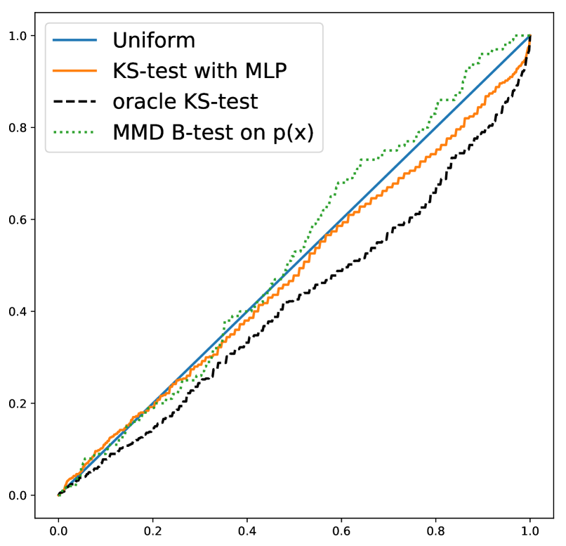
(a) CDF of $p$-value at $\delta=0$

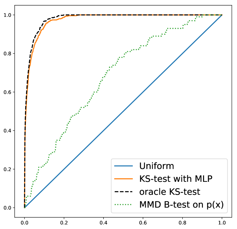
(b) CDF of $p$-value at $\delta=0.6$

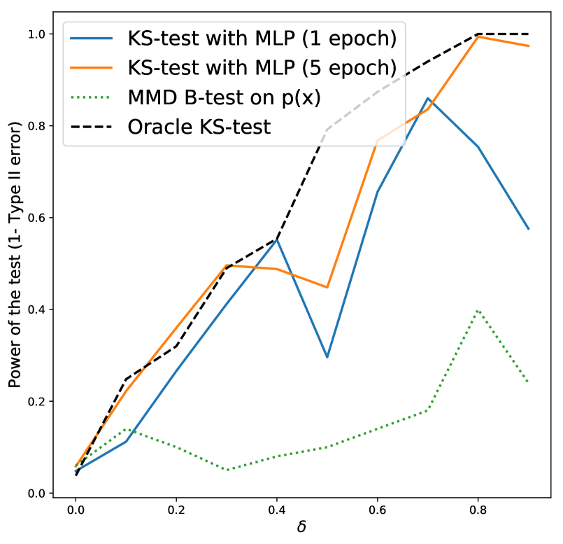
(c) Power at $\alpha=0.05$

Figure 1: Label-shift detection on MNIST. Pane 1(a) illustrates that Type I error is correctly controlled absent label shift. Pane 1(b) illustrates high power under mild label-shift. Pane 1(c) shows increased power for better classifiers. We compare to kernel two-sample tests (Zaremba et al., 2013) and an (infeasible) oracle two sample test that directly tests $p(y)=q(y)$ with samples from each. The proposed test beats directly testing in high-dimensions and nearly matches the oracle.

5.1 Black Box Shift Detection (BBSD)

Formally, detection can be cast as a hypothesis testing problem where the null hypothesis is $\mathbf{H}_{0}:q(y)=p(y)$ and the alternative hypothesis is that $\mathbf{H}_{1}:q(y)\neq p(y).$ Recall that we observe neither $q(y)$ nor any samples from it. However, we do observe unlabeled data from the target distribution and our predictor $f$.

Proposition 4 (Detecting label-shift).

Under Assumption A.1, A.2 and for each classifier $f$ satisfying A.3 we have that $q(y)=p(y)$ if and only if $p(\hat{y})=q(\hat{y})$.

Proof.

Plug $P$ and $Q$ into (1) and apply Lemma 1 with assumption A.1. The result follows directly from our analysis in the proof of Proposition 2 that shows $p(\hat{y},y)$ is invertible under the assumptions A.2 and A.3. ∎

Thus, under weak assumptions, we can test $\mathbf{H}_{0}$ by running two-sample tests on readily available samples from $p(\hat{y})$ and $q(\hat{y})$. Examples include the Kolmogorov-Smirnoff test, Anderson-Darling or the Maximum Mean Discrepancy. In all tests, asymptotic distributions are known and we can almost perfectly control the Type I error. The power of the test ($1$-Type II error) depends on the classifier’s performance on distribution $P$, thereby allowing us to leverage recent progress in deep learning to attack the classic problem of detecting non-stationarity in the data distribution.

One could also test whether $p(x)=q(x)$. Under the label-shift assumption this is implied by $q(y)=p(y)$. The advantage of testing the distribution of $f(\boldsymbol{x})$ instead of $\boldsymbol{x}$ is that we only need to deal with a one-dimensional distribution. Per theory and experiments in (Ramdas et al., 2015) two-sample tests in high dimensions are exponentially harder.

One surprising byproduct is that we can sometimes use this approach to detect covariate-shift, concept-shift, and more general forms of nonstationarity.

Proposition 5 (Detecting general nonstationarity).

For any fixed measurable $f:\mathcal{X}\rightarrow\mathcal{Y}$

$$P=Q\implies p(x)=q(x)\implies p(\hat{y})=q(\hat{y}).$$

This follows directly from the measurability of $f$.

While the converse is not true in general, $p(\hat{y})=q(\hat{y})$ does imply that for every measurable $\mathcal{S}\subset\mathcal{Y}$,

$$q(x\in f^{-1}(\mathcal{S}))=p(x\in f^{-1}(\mathcal{S})).$$

This suggests that testing $\hat{\mathbf{H}}_{0}:p(\hat{y})=q(\hat{y})$ may help us to determine if there’s sufficient statistical evidence that domain adaptation techniques are required.

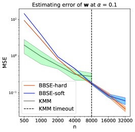
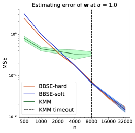
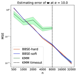
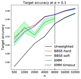
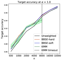
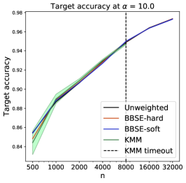
Figure 2: Estimation error (top row) and correction accuracy (bottom row) vs dataset size on MNIST data compared to KMM (Zhang et al., 2013) under Dirichlet shift (left to right) with $\alpha=\{.1,1.0,10.0\}$ (smaller $\alpha$ means larger shift). BBSE confidence interval on $20$ runs, KMM on $5$ runs due to computation; $n=8000$ is largest feasible KMM experiment.

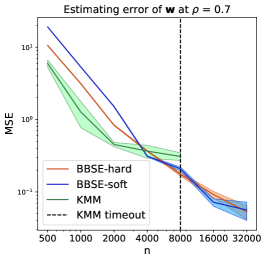
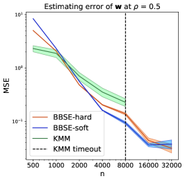
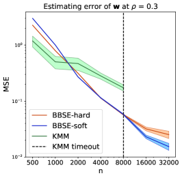
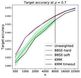
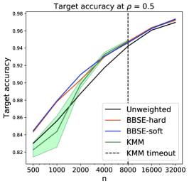
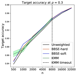
Figure 3: Label-shift estimation and correction on MNIST data with simulated tweak-one shift with parameter $\rho$.

5.2 Black Box Shift Correction (BBSC)

Our estimator also points to a systematic method of correcting for label-shift via importance-weighted ERM. Specifically, we propose the following algorithm:

Algorithm 1 Domain adaptation via Label Shift

0:   Samples from source distribution $X$, $\mathbf{y}$. Unlabeled data from target distribution $X^{\prime}$. A class of classifiers $\mathcal{F}$. Hyperparameter $0<\delta<1/k$.

  1. Randomly split the training data into two $X_{1},X_{2}\in\mathbb{R}^{n/2\times d}$ and $\boldsymbol{y}_{1},\boldsymbol{y}_{2}\mathbb{R}^{n/2}$.

  2. Use $X_{1},\boldsymbol{y}_{1}$ to train the classifier and obtain $f\in\mathcal{F}$.

  3. On the hold-out data set $X_{2},\boldsymbol{y}_{2}$, calculate the confusion matrix $\hat{\mathbf{C}}_{\hat{y},y}$. If ,

  if $\sigma_{\min}\left(\hat{\mathbf{C}}_{\hat{y},y}\right)\leq\delta$ then

     Set $\hat{\boldsymbol{w}}=\boldsymbol{1}$.

  else

     Estimate $\hat{\boldsymbol{w}}=\hat{\mathbf{C}}_{\hat{y},y}^{-1}\hat{\boldsymbol{\mu}}_{\hat{y}}$ .

  end if

  4. Solve the importance weighted ERM on the $X_{1},\boldsymbol{y}_{1}$ with $\max(\hat{\boldsymbol{w}},\boldsymbol{0})$ and obtain $\tilde{f}$. 

   $\tilde{f}$

Note that for classes that occur rarely in the test set, BBSE may produce negative importance weights. During ERM, a flipped sign would cause us to maximize loss, which is unbounded above. Thus, we clip negative weights to $0$.

Owing to its efficacy and generality, our approach can serve as a default tool to deal with domain adaptation. It is one of the first things to try even when the label-shift assumption doesn’t hold. By contrast, the heuristic method of using logistic-regression to construct importance weights (Bickel et al., 2009) lacks theoretical justification that the estimated weights are correct.

Even in the simpler problem of average treatment effect (ATE) estimation, it’s known that using estimated propensity can lead to estimators with large variance (Kang & Schafer, 2007). The same issue applies in supervised learning. We may prefer to live with the biased solution from the unweighted ERM rather than suffer high variance from an unbiased weighted ERM. Our proposed approach offers a consistent low-variance estimator under label shift.

6 Experiments

We experimentally demonstrate the power of BBSE with real data and simulated label shift. We organize results into three categories — shift detection with BBSD, weight estimation with BBSE, and classifier correction with BBSC. BBSE-hard denotes our method where $f$ yields classifications. In BBSE-soft, $f$ outputs probabilities.

Label Shift Simulation To simulate distribution shift in our experiments, we adopt the following protocols: First, we split the original data into train, validation, and test sets. Then, given distributions $p(y)$ and $q(y)$, we generate each set by sampling with replacement from the appropriate split. In knock-out shift, we knock out a fraction $\delta$ of data points from a given class from training and validation sets. In tweak-one shift, we assign a probability $\rho$ to one of the classes, the rest of the mass is spread evenly among the other classes. In Dirichlet shift, we draw $p(y)$ from a Dirichlet distribution with concentration parameter $\alpha$. With uniform $p(y)$, Dirichlet shift is bigger for smaller $\alpha$.

Label-shift detection We conduct nonparametric two-sample tests as described in Section 5.1 using the MNIST handwritten digits data set. To simulate the label-shift, we randomly split the training data into a training set, a validating set and a test set, each with 20,000 data points, and apply knock-out shift on class $y=5$ . Note that $p(y)$ and $q(y)$ differ increasingly as $\delta$ grows large, making shift detection easier. We obtain $f$ by training a two-layer ReLU-activated Multilayer Perceptron (MLP) with 256 neurons on the training set for five epochs. We conduct a two-sample test of whether the distribution of $f(\text{Validation Set})$ and $f(\text{Test Set})$ are the same using the Kolmogorov-Smirnov test. The results, summarized in Figure 1, demonstrate that BBSD (1) produces a $p$-value that distributes uniformly when $\delta=0$ (2) provides more power (less Type II error) than the state-of-the-art kernel two-sample test that discriminates $p(\boldsymbol{x})$ and $q(\boldsymbol{x})$ at $\delta=0.5$, and (3) gets better as we train the black-box predictor even more.

Weight estimation and label-shift correction We evaluate BBSE on MNIST by simulating label shift and datasets of various sizes. Specifically, we split the training data set randomly in two, using first half to train $f$ and the second half to estimate $\boldsymbol{w}$. We use then use the full training set for weighted ERM. As before, $f$ is a two-layer MLP. For fair comparisons with baselines, the full training data set is used throughout (since they do not need $f$ without data splitting). We evaluate our estimator $\hat{\boldsymbol{w}}$ against the ground truth $\boldsymbol{w}$ and by the prediction accuracy of BBSC on the test set. To cover a variety of different types of label-shift, we take $p(y)$ as a uniform distribution and generate $q(y)$ with Dirichlet shift for $\alpha=0.1,1.0,10.0$ (Figure 2).

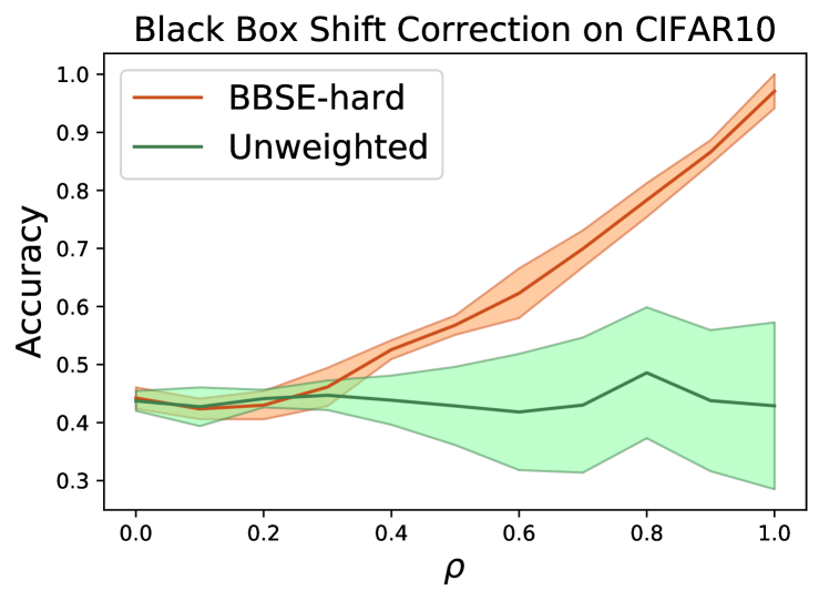
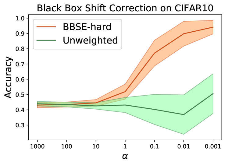
Figure 4: Accuracy of BBSC on CIFAR 10 with (top) tweak-one shift and (bottom) Dirichlet shift.

Label-shift correction for CIFAR10 Next, we extend our experiments to the CIFAR dataset, using the same MLP and this time allowing it to train for 10 epochs. We consider both tweak-one and Dirichlet shift, and compare BBSE to the unweighted classifier under varying degrees of shift (Figure 4). For the tweak-one experiment, we try $\rho\in\{0.0,0.1,...,1.0\}$, averaging results over all 10 choices of the tweaked label, and plotting the variance. For the Dirichlet experiments, we sample $20$ $q(y)$ for every choice of $\alpha$ in the range {1000, 100, …, .001}. Because kernel-based baselines cannot handle datasets this large or high-dimensional, we compare only to unweighted ERM.

Kernel mean matching (KMM) baselines We compare BBSE to the state-of-the-art kernel mean matching (KMM) methods. For the detection experiments (Figure 1), our baseline is the kernel B-test (Zaremba et al., 2013), an extension of the kernel max mean discrepancy (MMD) test due to Gretton et al. (2012) that boasts nearly linear-time computation and little loss in power. We compare BBSE to a KMM approach Zhang et al. (2013), that solves

$$\min_{\boldsymbol{w}}\|\mathbf{C}_{\boldsymbol{x}|y}(\boldsymbol{\nu}_{y}\circ\boldsymbol{w})-\boldsymbol{\mu}_{\boldsymbol{x}}\|_{\mathcal{H}}^{2},$$

where we use operator $\mathbf{C}_{\boldsymbol{x}|y}:=\mathbb{E}[\phi(\boldsymbol{x})|\psi(y)]$ and function $\boldsymbol{\mu}_{x}:=\mathbb{E}_{Q}[\phi(\boldsymbol{x})]$ to denote the kernel embedding of $p(\boldsymbol{x}|y)$ and $p_{Q}(x)$ respectively. Note that under the label-shift assumption, $\mathbf{C}_{\boldsymbol{x}|y}$ is the same for $P$ and $Q$. Also note that since $\mathcal{Y}$ is discrete, $\psi(y)$ is simply the one-hot representation of $y$, so $\boldsymbol{\nu}_{y}$ is the same as our definition before and $\mathbf{C}_{\boldsymbol{x}|y}$, $\boldsymbol{\nu}_{y}$ and $\boldsymbol{\mu}_{\boldsymbol{x}}$ must be estimated from finite data. The proposal involves a constrained optimization by solving a Gaussian process regression with automatic hyperparameter choices through marginal likelihood.

For fair comparison, we used the original authors’ implementations as baselines and also used the median trick to adaptively tune the RBF kernel’s hyperparameter. A key difference is that BBSE matches the distribution of $\hat{y}$ rather than distribution of $\boldsymbol{x}$ like (Zhang et al., 2013) and we learn $f$ through supervised learning rather than by specifying a feature map $\phi$ by choosing a kernel up front.

Note that KMM, like many kernel methods, requires the construction and inversion of an $n\times n$ Gram matrix, which has complexity of $O(n^{3})$. This hinders its application to real-life machine learning problems where $n$ will often be 100s of thousands. In our experiments, we find that the largest $n$ for which we can feasibly run the KMM code is roughly $8,000$ and that is where we unfortunately have to stop for the MNIST experiment. For the same reason, we cannot run KMM for the CIFAR10 experiments. The MSE curves in Figure 2 for estimating $\boldsymbol{w}$ suggest that the convergence rate of KMM is slower than BBSE by a polynomial factor and that BBSE better handles large datasets.

7 Discussion

Constructing the training Set The error bounds on our estimates depend on the norm of the true vector $w(y):=q(y)/p(y)$. This confirms the common sense that absent any assumption on $q(y)$, and given the ability to select class-conditioned examples for annotations one should build a dataset with uniform $p(y)$. Then it’s always possible to apply BBSE successfully at test time to correct $f$.

Sporadic Shift In some settings, $p(y)$ might change only sporadically. In these cases, when no label shift occurs, applying BBSC might damage the classifier. For these cases, we prose to combine detection and estimation, correcting the classifier only when a shift has likely occurred.

Using known predictor In our experiments, $f$ has been trained using a random split of the data set, which makes BBSEto perform worse than baseline when the data set is extremely small. In practice, especially in the context of web services, there could be a natural predictor $f$ that is currently being deployed whose training data were legacy and have little to do with the two distributions that we are trying to distinguish. In this case, we do not lose that factor of $2$ and we do not suffer from the variance in training $f$ with a small amount of data. This could allow us to detect mild shift in distributions in very short period of time. Making it suitable for applications such as financial market prediction.

BBSE with degenerate confusion matrices In practice, sometime confusion matrices will be degenerate. For instance, when a class $i$ is rare under $P$, and the features are only partially predictive, we might find that $p(f(\boldsymbol{x})=i)=0$. In these cases, two straightforward variations on the black box method may still work: First, while our analysis focuses on confusion matrices, it easily extends to any operator $f$, such as soft probabilities. If each class $i$, even if $i$ is never the argmax for any example, so long as $p(\hat{y}=i|y=i)>p(\hat{y}=i|y=j)$ for any $j\neq i$, the soft confusion matrix will be invertible. Even when we produce and operator with an invertible confusion matrix, two options remain: We can merge $c$ classes together, yielding a $(k-c)\times(k-c)$ invertible confusion matrix. While we might not be able to estimate the frequencies of those $c$ classes, we can estimate the others accurately. Another possibility is to compute the pseudo-inverse.

Future Work As a next step, we plan to extend our methodology to the streaming setting. In practice, label distributions tend to shift progressively, presenting a new challenge: if we apply BBSE on trailing windows, then we face a trade-off. Looking far back increases $m$, lowering estimation error, but the estimate will be less fresh. The use of propensity weights $w$ on $y$ makes BBSE amenable to doubly-robust estimates, the typical bias-variance tradeoff, and related techniques, common in covariate shift correction.

Appendix A Additional discussion

In this section we provide a few answers to some questions people may have when using our proposed techniques.

What if the label-shift assumption does not hold?

In many applications, we do not know whether label-shift is a reasonable assumption or not. In particular, whenever there are unobserved variables that affects both $\boldsymbol{x}$ and $y$, then neither label-shift nor covariate-shift is true. However, label shift could still be a good approximation in the in the finite sample environment. Luckily, we can test whether the label-shift assumption is a good approximation in a data-driven fashion via the kernel two-sample tests. In particular, let $\phi:\mathcal{X}\rightarrow\mathcal{F}$ be an arbitrary feature map that (possibly reduces the dimension of $\boldsymbol{x}$) and $k:\mathcal{F}\times\mathcal{F}\rightarrow\mathbb{R}$ be the kernel function that induces a RKHS $\mathcal{H}$. Let $\boldsymbol{w}=[q(y)/p(y)]_{y=1,...,k}$, then

$$\mathbb{E}_{p}\left[\boldsymbol{w}(y)k(\phi(\boldsymbol{x}),\cdot)\right]=\mathbb{E}_{q}\left[k(\phi(\boldsymbol{x}),\cdot)\right].$$

The LHS can be estimated by plugging in $\hat{\boldsymbol{w}}$ and a stochastic approximation of the expectation using labeled data from the source domain and the RHS can be estimated by the sample mean using unlabeled data from the target domain. In particular, if label-shift assumption is true or a good approximation, then

$$\|\frac{1}{n}\sum_{i=1}^{n}\left[\hat{\boldsymbol{w}}(y_{i})k(\phi(\boldsymbol{x}_{i}),\cdot)\right]-\frac{1}{m}\sum_{j=1}^{m}k(\phi(\boldsymbol{x}^{\prime}_{j}),\cdot)\|_{\mathcal{H}}^{2}$$

should be on the same order as the statistical error that we can calculate by $m,n$ and the error of $\hat{\boldsymbol{w}}$ in estimating $\boldsymbol{w}$.

Model selection criterion and the choice of $f$.

Our analysis assumes that $f$ is fixed and given, but in practice, often we need to train $f$ from the same data set. Given a number of choices, one may wonder which blackbox predictor $f$ should we prefer out of a collection of $\mathcal{F}$? Our theoretical results suggest a natural quantity: the smallest singular value of the confusion matrix, for choosing the blackbox predictors. Note that the smallest singular value is a quantity that can be estimated using only labeled data from the source domain. Therefore a practical heuristic to use is to the $f$ that maximizes the smallest singular value of the corresponding $\hat{C}_{f}$. Figure 5 plots the smallest singular value of the confusion matrices as the number of epochs of training $f$ gets larger. The model we use is the same multi-layer perceptron that we used for our experiments and the source distribution is one that we knocks off 80% of the fifth class. This is the same model and data set we used in Figure 1(c). Referring to $\delta=0.8$ in Figure 1(c), we see that the test power of $f$ that is trained for only one epoch is much lower than the $f$ that is trained for five epochs, and the gap in the smallest singular values is predicative of the fact at least qualitatively.

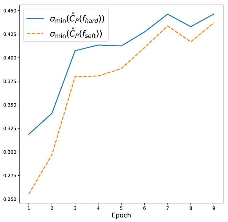
Figure 5: The smallest singular value of the estimated confusion matrix: $\hat{C}_{f}$ under distribution $p$ as a function of the number of epochs we train the classifiers on.

Is data splitting needed?

Recall that we train the model $f$ and estimate $\boldsymbol{w}$ using two independent splits of the labeled data set drawn from the same distribution. In practice, especially when $n$ is large, using the same data to train $f$ and to estimate $\boldsymbol{w}$ will be more data efficient. This comes at a price of a small bias. It is unclear how to quantify that bias but the data-reuse version could be useful in practice as a heuristic.

Appendix B Proofs

We present the proofs of Lemma 1 and Proposition 2 in this Appendix.

Proof of Lemma 1.

By the law of total probability

$$q(\hat{y}|y)=\sum_{y\in\mathcal{Y}}q(\hat{y}|\boldsymbol{x},y)q(\boldsymbol{x}|y)=\sum_{y\in\mathcal{Y}}q(\hat{y}|\boldsymbol{x},y)p(\boldsymbol{x}|y)$$

$$=\sum_{y\in\mathcal{Y}}p_{f}(\hat{y}|\boldsymbol{x})p(\boldsymbol{x}|y)=\sum_{y\in\mathcal{Y}}p(\hat{y}|\boldsymbol{x},y)p(\boldsymbol{x}|y)=p(\hat{y}|y).$$

We applied A.1 to the second equality, and used the conditional independence $\hat{y}\mathchoice{\mathrel{\hbox to0.0pt{$\displaystyle\perp$\hss}\mkern 2.0mu{\displaystyle\perp}}}{\mathrel{\hbox to0.0pt{$\textstyle\perp$\hss}\mkern 2.0mu{\textstyle\perp}}}{\mathrel{\hbox to0.0pt{$\scriptstyle\perp$\hss}\mkern 2.0mu{\scriptstyle\perp}}}{\mathrel{\hbox to0.0pt{$\scriptscriptstyle\perp$\hss}\mkern 2.0mu{\scriptscriptstyle\perp}}}y|x$ under $P$ and $Q$ together with $p(\hat{y}|\boldsymbol{x})$ being determined by $f$, which is fixed. ∎

Proof of Proposition 2.

A.2 ensures that $\boldsymbol{w}<\infty$. By Assumption A.3, ${\mathbf{C}}_{\hat{y},y}$ is invertible. Let $\delta>0$ be its smallest singular value. We bound the probability that $\hat{\mathbf{C}}_{\hat{y},y}$ is not invertible:

$$\mathbb{P}(\hat{\mathbf{C}}_{\hat{y},y}\text{ is not invertible})\leq\mathbb{P}(\sigma_{\min}(\hat{\mathbf{C}}_{\hat{y},y})<\delta/2)$$

$$\leq\mathbb{P}(\|\hat{\mathbf{C}}_{\hat{y},y}-\mathbf{C}_{\hat{y},y}\|_{2}\geq\delta/2)\underset{\mathclap{\overset{\uparrow}{\text{pigeon hole}}}}{\leq}\mathbb{P}(\|\hat{\mathbf{C}}_{\hat{y},y}-\mathbf{C}_{\hat{y},y}\|_{F}\geq\frac{\delta}{2\sqrt{k}})$$

$$\underset{\mathclap{\overset{\uparrow}{\text{pigeon hole}}}}{\leq}\mathbb{P}(\exists(i,j)\in[k]^{2},\text{ s.t.}|[\hat{\mathbf{C}}_{\hat{y},y}]_{i,j}-[\mathbf{C}_{\hat{y},y}]_{i,j}|\geq\frac{\delta}{2k^{1.5}})\underset{\mathclap{\overset{\uparrow}{\text{Hoeffding}}}}{\leq}2e^{-\frac{n\delta^{2}}{4k^{3}}}.$$

By the convergence of geometric series $\sum_{n}\mathbb{P}(\hat{\mathbf{C}}_{\hat{y},y}\text{ is not invertible})<+\infty$. This allows us to invoke the First Borel-Cantelli Lemma, which shows

$$\mathbb{P}(\hat{\mathbf{C}}_{\hat{y},y}\text{ is not invertible}\text{ i.o.})=0.$$ (6)

This ensures that as $n\rightarrow\infty$, $\hat{\mathbf{C}}_{\hat{y},y}$ is invertible almost surely. By the strong law of large numbers (SLLN), as $n\rightarrow\infty$ $\hat{\mathbf{C}}_{\hat{y},y}\overset{\text{a.s.}}{\longrightarrow}\mathbf{C}_{\hat{y},y}$ and $\hat{\boldsymbol{\nu}}_{y}\overset{\text{a.s.}}{\longrightarrow}\boldsymbol{\nu}_{y}$. Similarly, as $m\rightarrow\infty$, $\hat{\boldsymbol{\mu}}_{\hat{y}}\overset{\text{a.s.}}{\longrightarrow}\boldsymbol{\mu}_{\hat{y}}$. Combining these with (6) and applying the continuous mapping theorem with the fact that the inverse of an invertible matrix is a continuous mapping we get that

$$\hat{\boldsymbol{w}}=[\hat{\mathbf{C}}_{\hat{y},y}]^{-1}\hat{\boldsymbol{\mu}}_{\hat{y}}\overset{\text{a.s.}}{\longrightarrow}\boldsymbol{w},\text{ and }\hat{\boldsymbol{\mu}}_{y}=\mathrm{diag}(\hat{\boldsymbol{\nu}}_{y})\hat{\boldsymbol{w}}\overset{\text{a.s.}}{\longrightarrow}\boldsymbol{\mu}_{y}.$$

∎

Appendix C Concentration inequalities

Lemma 6 (Hoeffding’s inequality).

Let $x_{1},...,x_{n}$ be independent random variables bounded by $[a_{i},b_{i}]$. Then $\bar{x}=\frac{1}{n}\sum_{i=1}^{n}x_{i}$ obeys for any $t>0$

$$\mathbb{P}(\left|\bar{x}-\mathbb{E}[\bar{x}]\right|\geq t)\leq 2\exp\left(-\frac{2n^{2}t^{2}}{\sum_{i=1}^{n}(b_{i}-a_{i})^{2}}\right).$$

Lemma 7 (Matrix Bernstein Inequality (rectangular case)).

Let $\mathbf{Z}_{1},...,\mathbf{Z}_{n}$ be independent random matrices with dimension $d_{1}\times d_{2}$ and each satisfy

$$\mathbb{E}\mathbf{Z}_{i}=\mathbf{0}\text{ and }\|\mathbf{Z}_{i}\|\leq R$$

almost surely. Define the variance parameter

$$\sigma^{2}-\max\{\|\sum_{i}\mathbb{E}[\mathbf{Z}_{i}\mathbf{Z}_{i}^{T}]\|,\|\sum_{i}\mathbb{E}[\mathbf{Z}_{i}^{T}\mathbf{Z}_{i}]\|\}.$$

Then for all $t\geq 0$,

$$\mathbb{P}\left(\|\sum_{i}\mathbf{Z}_{i}\|\geq t\right)\leq(d_{1}+d_{2})\cdot e^{\frac{-t^{2}}{\sigma^{2}+Rt/3}}.$$

References

- Bickel et al. (2009) Bickel, S., Brückner, M., & Scheffer, T. (2009). Discriminative learning under covariate shift. Journal of Machine Learning Research, 10(Sep), 2137–2155.
- Bishop (1995) Bishop, C. M. (1995). Neural networks for pattern recognition. Oxford university press.
- Buck et al. (1966) Buck, A., Gart, J., et al. (1966). Comparison of a screening test and a reference test in epidemiologic studies. ii. a probabilistic model for the comparison of diagnostic tests. American Journal of Epidemiology.
- Chan & Ng (2005) Chan, Y. S., & Ng, H. T. (2005). Word sense disambiguation with distribution estimation. In Proceedings of the 19th international joint conference on Artificial intelligence, (pp. 1010–1015). Morgan Kaufmann Publishers Inc.
- Deng et al. (2009) Deng, J., Dong, W., Socher, R., Li, L.-J., Li, K., & Fei-Fei, L. (2009). Imagenet: A large-scale hierarchical image database. In CVPR.
- Elkan (2001) Elkan, C. (2001). The foundations of cost-sensitive learning. In IJCAI.
- Forman (2008) Forman, G. (2008). Quantifying counts and costs via classification. Data Mining and Knowledge Discovery.
- Gretton et al. (2012) Gretton, A., Borgwardt, K. M., Rasch, M. J., Schölkopf, B., & Smola, A. (2012). A kernel two-sample test. Journal of Machine Learning Research, 13(Mar), 723–773.
- Gretton et al. (2009) Gretton, A., Smola, A. J., Huang, J., Schmittfull, M., Borgwardt, K. M., & Schölkopf, B. (2009). Covariate shift by kernel mean matching. Journal of Machine Learning Research.
- Heckman (1977) Heckman, J. J. (1977). Sample selection bias as a specification error (with an application to the estimation of labor supply functions).
- Huang et al. (2007) Huang, J., Gretton, A., Borgwardt, K. M., Schölkopf, B., & Smola, A. J. (2007). Correcting sample selection bias by unlabeled data. In Advances in neural information processing systems.
- Kang & Schafer (2007) Kang, J. D., & Schafer, J. L. (2007). Demystifying double robustness: A comparison of alternative strategies for estimating a population mean from incomplete data. Statistical science, 22(4), 523–539.
- Manski & Lerman (1977) Manski, C. F., & Lerman, S. R. (1977). The estimation of choice probabilities from choice based samples. Econometrica: Journal of the Econometric Society.
- Ramdas et al. (2015) Ramdas, A., Reddi, S. J., Póczos, B., Singh, A., & Wasserman, L. A. (2015). On the decreasing power of kernel and distance based nonparametric hypothesis tests in high dimensions. In AAAI, (pp. 3571–3577).
- Rosenbaum & Rubin (1983) Rosenbaum, P. R., & Rubin, D. B. (1983). The central role of the propensity score in observational studies for causal effects. Biometrika, 70(1), 41–55.
- Saerens et al. (2002) Saerens, M., Latinne, P., & Decaestecker, C. (2002). Adjusting the outputs of a classifier to new a priori probabilities: a simple procedure. Neural computation, 14(1), 21–41.
- Schölkopf et al. (2012) Schölkopf, B., Janzing, D., Peters, J., Sgouritsa, E., Zhang, K., & Mooij, J. (2012). On causal and anticausal learning. In International Coference on International Conference on Machine Learning (ICML-12), (pp. 459–466). Omnipress.
- Shimodaira (2000) Shimodaira, H. (2000). Improving predictive inference under covariate shift by weighting the log-likelihood function. Journal of statistical planning and inference.
- Storkey (2009) Storkey, A. (2009). When training and test sets are different: characterizing learning transfer. Dataset shift in machine learning.
- Sugiyama et al. (2008) Sugiyama, M., Nakajima, S., Kashima, H., Buenau, P. V., & Kawanabe, M. (2008). Direct importance estimation with model selection and its application to covariate shift adaptation. In Advances in neural information processing systems.
- Zadrozny (2004) Zadrozny, B. (2004). Learning and evaluating classifiers under sample selection bias. In Proceedings of the twenty-first international conference on Machine learning, (p. 114). ACM.
- Zaremba et al. (2013) Zaremba, W., Gretton, A., & Blaschko, M. (2013). B-test: A non-parametric, low variance kernel two-sample test. In Advances in neural information processing systems, (pp. 755–763).
- Zhang et al. (2013) Zhang, K., Schölkopf, B., Muandet, K., & Wang, Z. (2013). Domain adaptation under target and conditional shift. In International Conference on Machine Learning, (pp. 819–827).
- Zhu et al. (2010) Zhu, X., Gibson, B. R., Jun, K.-S., Rogers, T. T., Harrison, J., & Kalish, C. (2010). Cognitive models of test-item effects in human category learning. In ICML.