Measurement of the intensity ratio of Auger and conversion electrons for the electron capture decay of ¹²⁵I

Abstract

Auger electrons emitted after nuclear decay have potential application in targeted cancer therapy. For this purpose it is important to know the Auger electron yield per nuclear decay. In this work we describe a measurement of the ratio of the number of conversion electrons (emitted as part of the nuclear decay process) to the number of Auger electrons (emitted as part of the atomic relaxation process after the nuclear decay) for the case of ¹²⁵I. Results are compared with Monte-Carlo type simulations of the relaxation cascade using the BrIccEmis code. Our results indicate that for ¹²⁵I the calculations based on rates from the Evaluated Atomic Data Library (EADL) underestimate the K Auger yields by 20%.

• February 2018

1 Introduction

Low energy (10-1000 eV) electrons have a very small mean free path (of the order of nm) for inelastic excitations. The corresponding high linear energy transfer (LET) values are attractive if one aims to target tumour cells without collateral damage to neighbouring healthy cells. A convenient source of low energy electrons is Auger electron emission after nuclear decay, and their use in tumour therapy has been discussed extensively (Kassis, 2004; Tavares and Tavares, 2010; Cornelissen and Vallis, 2010; Rezaee et al., 2017).

After nuclear decay the atom is often left with inner-shell vacancies and this excited state will decay to the ground state by emission of a number of Auger electrons and X-rays. There are usually few Auger electrons with energies of 20-30 keV and a corresponding range of $\approx 10$ $\mu$m. The vast majority of Auger electrons have much lower energies, below 1 keV down to almost zero energy. The size of a normal mammalian cell is $\approx$ 10 $\mu$m, thus the effects of a specific decay are almost always limited to a single cell. Due to this short range, Auger emitters are expected to be particularly effective when they are located in the nucleus of a tumour cell as then the probability of double-strand breaking of the DNA is very high, preventing the cell from multiplying (Falzone et al., 2017).

To exploit their use in nuclear medicine it is thus imperative to have precise knowledge of the full energy spectrum of the Auger electrons emitted per nuclear decay. Atomic relaxation (the return of an atom with an inner core hole to its ground state) is a complex process with many possible pathways, especially for higher atomic numbers. The problem is most conveniently tackled using Monte Carlo simulations based on decay rates as calculated for isolated atoms (Pomplun et al., 1987; Stepanek, 2000; Nikjoo et al., 2008; Lee et al., 2016). Experimental verification of such results, i.e. the predicted number of Auger electrons produced per nuclear decay is then highly desirable.

The two nuclear decay processes producing inner-shell vacancies are electron capture and internal conversion. The probability of internal conversion involving inner shell electrons is usually known within a percent (Kibédi et al., 2008). By comparing the conversion electron (CE) and Auger intensity one can benchmark the Monte Carlo simulations. Such is the aim of this paper.

¹²⁵I was chosen for the following reasons. It is one of the most extensively studied radioisotope owing to its possible application to cancer therapy (Balagurumoorthy et al., 2012). Very recently, in combination with gold nanorparticles, ¹²⁵I was used for targeted imaging and radionuclide therapy (Clanton et al., 2018). In the present study we used ¹²⁵I to measure the ratio of Auger to conversion electrons. ¹²⁵I decays with a half-life of 59.5 days via electron capture to an excited state of the ¹²⁵Te nucleus. This excited state decays in 93% of the cases to its ground state by the emission of a CE. The half-life of this excited state is 1.48 ns, which is much longer than the time scale for atomic relaxation (femtoseconds). There are thus two separate relaxation cascades contributing to the Auger yield: one after electron capture and the other after emission of a CE. The combined large Auger yield makes ¹²⁵I an attractive candidate for targeted tumour therapy.

2 Experimental Details

¹²⁵I can be prepared as a sub-monolayer source on a Au(111) surface which is stable in air (Huang et al., 1997) and the Te atoms, produced in the decay process, are bound to this surface as well (Pronschinske et al., 2016). Samples with a third of a monolayer of ¹²⁵I on a Au(111) surface were prepared as described by Pronschinske et al. (2015). Au(111) surfaces were obtained by flame annealing Au samples (Arrandee Metal GMBH, Germany) just before the ¹²⁵I deposition. A droplet containing NaI in a NaOH solution (pH $\approx 10$, Perkin Elmer) was put on this surface, and left to react. An approximately 4 mm diameter source with a strength of 4 MBq was obtained.

The measurements were performed with two spectrometers. For energies below 4 keV (LMM Auger and K CE ), the DESA100 SuperCMA (Staib Instruments) was used. The spectrometer was slightly modified by incorporating high-$Z$ metal shielding to prevent X-rays emitted by the sample interacting with the channeltron detector. The second spectrometer was locally-built and measures electrons with higher energies up to 40 keV (the KLL Auger and L CE) (Vos et al., 2000; Went and Vos, 2005). This spectrometer has a smaller opening angle, but it is equipped with a two-dimensional detector, measuring a range of energies simultaneously (17% of the pass energy of 1 keV). For both spectrometers the Auger signal is on top of a background due to the dark count rate of the detector, which did not depend on the electron energy being measured.

As the Auger energies are different from the CE energies, it is essential to understand how the spectrometers efficiency varies with the electron energy $E$. The efficiency of the DESA100 was determined experimentally before (Gergely et al., 1999) and for energies higher than a few times its pass energy, those results indicate an efficiency that scales as $1/E^{1.2}$. Our SIMION electron optics simulations (Dahl, 2000) suggest a somewhat weaker dependence (proportional to $\approx 1/E^{0.8}$). In the analysis presented here a simple $1/E$ dependence was used. As the main LMM Auger line energies differ by less than 20% from the K-CE electron energy the CE to Auger intensity ratio is only affected on a 5% level if a $1/E^{0.8}$ or a $1/E^{1.2}$ dependence is assumed instead of a simple $1/E$ dependence. The high-energy spectrometer uses a lens stack behind a 0.5 mm wide slit. It decelerates the electrons and focuses them at the entrance of an hemispherical analyser. SIMION simulations showed that all electrons transmitted through the slit will enter the analyser. The spectrometer transmission is thus determined solely by the width of the entrance slit and is independent of $E$. The fact that the L-shell CEs have $\approx$ 30% higher energy than the KLL Auger electrons should thus not affect the comparison of their intensities.

3 Results

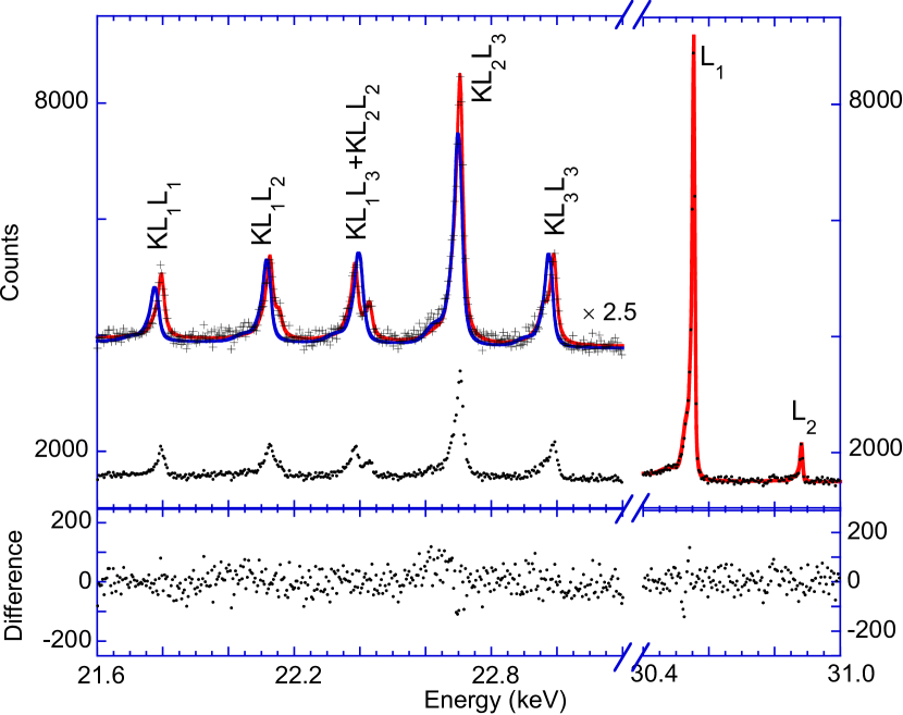
Figure 1: The KLL Auger and L₁, L₂-CE spectrum as measured in a single run. The red line shows a fit of the KLL spectrum with 8 peaks following the approach of Larkins (1977) (residuals in lower panel). The blue line shows a description of the KLL spectrum based on the BrIccEmis calculation(Lee et al., 2016) which was scaled such that the calculated L₁ CE line has the same area as the measured one. The calculated Auger spectrum, normalised in this way, has an area that is smaller than the observed one.

3.1 High-Energy Auger

The KLL Auger spectrum together with the L₁ and L₂-CE line is shown in Fig. 1. The Auger part of the spectrum is similar to those obtained with a magnetic spectrometer by Graham et al. (1962). The KLL Auger spectrum consists of several peaks. There are (at least) two ways to describe this spectrum:
(i) One can characterize each final state in terms of the atomic orbitals they originate from and to the total angular momentum and total spin quantum number of the final state. This leads to 9 possible final states in the intermediate coupling scheme. This approach was followed by Larkins (1977) and works well for two core holes, but becomes cumbersome when more vacancies are present, later in the cascade.
(ii) One can neglect the fine splitting and characterize the final state in terms of L_1,2,3 only. Then there are 6 possible final states but for Te the KL₁L₃ and KL₂L₂ energies are almost identical and experimentally not resolved. This approach is adopted in BrIccEmis (Lee et al., 2016) and remains manageable when one calculates several steps down in the relaxation cascade, when more vacancies are present.

A comparison was made with the peak positions as calculated by Larkins (1977) and the intensity as calculated by Chen et al. (1980), as shown in Fig. 1 as well. The lines were slightly asymmetric and each line was fitted with 4 Gaussians and a very small Shirley-type background (Shirley, 1972). The parameters used for this fit i.e. the energy offset (relative to the main peak), width and relative amplitude were the same for all lines (Auger and CE). The sum of the four Gaussians was convoluted with a Lorentzian, representing the lifetime broadening. For the Auger peak the lifetime broadening was taken to be the sum of the lifetime broadening of the K level and two L levels, for the CE peak just the L lifetime broadening was included. K and L lifetimes were taken from Krause and Oliver (1979). There were clearly 8 different components in the experimental KLL Auger spectrum. In some cases the calculated energies were separated by less than the peak width (determined mainly by lifetime broadening) and these components were taken together. The energy separation of the different components was within 10 eV of those calculated by Larkins (1977) and the relative intensity of the different components was close (within 3% of the intensity of the KL₂L₃ component) to those calculated by Chen et al. (1980). The intensity ratio of the L₁ CE line to the KL₂L₃ Auger line obtained from this fit was $1:0.61\pm 0.01$.

The BrIccEmis program (Lee et al., 2016) was used to describe the data. It uses nuclear decay data from ENSDF (https://www.nndc.bnl.gov/ensdf/), electron capture rates (Schönfeld, 1998), theoretical conversion coefficients (Kibédi et al., 2008) and atomic transition rates from EADL (Perkins et al., 1991). The L₁ CE to KL₂L₃ Auger intensity ratio, as calculated by BrIccEmis, is 1: 0.53 which is clearly lower than the experimentally observed one.

3.2 Low-Energy Auger

The K CEs have an energy of 3.679 keV. This energy is within the range of the LMM Auger transitions and one can again measure the ratio of CE and Auger intensities experimentally. A spectrum is shown in Fig. 2, and the peaks are somewhat sharper than those obtained by Casey and Albridge (1969) using a magnetic spectrometer. The strongest line is the K-CE line. There is some overlap between this line and neighbouring Auger lines. This close proximity makes corrections due to the energy dependence of the analyser efficiency small. It, however, makes it more difficult to assess the exact line shape. Clearly there is again a tail at the low energy side, but the K CE line is broader than the L₁-CE one, shown in Fig 1. This is at least in part due to the larger lifetime broadening of the K hole ($\approx 9.6$ eV versus 3.32 eV for the L₁ hole (Krause and Oliver, 1979)).

An attempt was made to fit the K conversion spectra with the same line shape as the L₁ conversion line (taking into account their different lifetime broadening), but this approach was unsuccessful, likely due to stronger interactions of the lower-energy electrons with their environment. Adjusting the line shape by increasing the intensity extending to lower energies (the tail) to get a better description, and using the same tail for the K CE line and nearby Auger lines (and a theoretical estimate of their lifetimes), we obtain the description of the spectrum based on BrIccEmis shown in Fig. 2. Theory was scaled so that the area of the K-CE line was the same as the experimental K-CE peak area. The Shirley-type background at lower energies is now more pronounced, indicating that the lower energy electrons interact more heavily with the substrate. However, this procedure showed that the Auger intensity (relative to the K-CE intensity) was underestimated by $\approx 20$% in the BrIccEmis calculation. This ratio is affected by uncertainties in the spectrometer response and by the procedures used to specify the line shape. Adjusting the line shape by extending the tail up to 300 eV below the main line (and reducing the contribution of the Shirley background at the same time) improves the agreement somewhat, but the calculated Auger intensity remains at least 10% lower than the experiment.

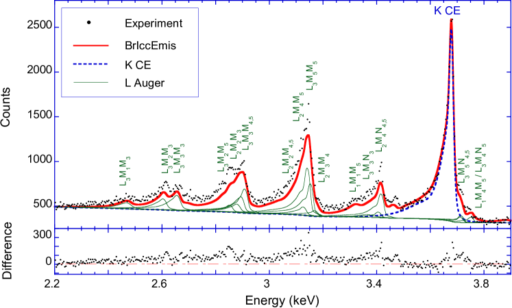
Figure 2: The measured spectrum (dots) of the K-CE and LMM Auger electrons. The solid red line is the calculated spectrum based on BrIccEmis scaled to the K-CE line. The contribution of the conversion electrons (blue, dashed line) and the strongest individual Auger electron contributions (thin green lines) are indicated as well. The lower panel shows the residual of the fit and the non-zero difference indicate that the theory underestimates the Auger intensity, relative to the CE intensity.

4 Conclusion and Discussion

The combined K CE - LMM Auger measurement indicates that the experimental relative Auger intensity is about 15-20%  higher than the calculated one. The same order of magnitude of difference was found for the KLL Auger intensity compared to the L₁-CE intensity, in spite of the fact that the energies involved were rather different and that two different spectrometers were used.

A core hole can either decay by X-ray emission (fluorescence) or by Auger decay. The K fluorescence yield, $\omega_{K}$ is defined as the fraction of K core holes that relaxes by X-ray emission. For the Te K shell, the adopted value based on experimental data $\omega_{K}$ is $\approx 87.5$% (Hubbell et al., 1994; Krause, 1979). The EADL database used by BrIccEmis (Perkins et al., 1991) uses a very similar value (87.9%). Some experimental values for Te are considerably smaller (82.3$\pm 7.3$%, (Singh et al., 1990)). The K-shell Auger yield is equal to (1- $\omega_{K}$). The corresponding Auger yield for the K shell based on theory would be 12.5%, whereas the results of Singh et al. (1990) correspond to an Auger yield of 17.7%, i.e. the measured fluorescence value from Singh would predict a 50% larger Auger yield, a difference much larger than what is required to describe our data. There is thus no experimental evidence that excludes the possibility that $\omega_{K}\approx 85$%, which would describe our data well. For high $Z$ elements, where $\omega_{k}$ approaches 1, the determination of the K Auger yield is thus an accurate way of determining the value of $\omega_{K}$.

	Auger electrons per decay
Transition	BrIccEmis	BrIccEmis	Stepanek	Pomplum
		mod. $\omega_{K}$
KLL	0.130	0.155	0.126	0.134
KXY	0.194	0.232	0.189	0.196
LMM	1.22	1.24	1.22	1.25
LXY	1.86	1.89	1.83	1.88

Table 1: The calculated K and L Auger transition rates based on BrIccEmis with the EADL $\omega_{K}$ value, with a modified $\omega_{K}$ value to reproduce the experimental KLL intensity and those obtained in the literature by Stepanek (2000) and Pomplun et al. (1987). Only the K Auger line intensity depends critically on the $\omega_{K}$ value used.

Besides the aforementioned fluorescence-yield measurements based on results from stable Te isotopes, there are earlier measurements based on coincidences between $\gamma$ and X-rays for the case of the decay of ¹²⁵I (Karttunen et al., 1969), which gave a value of the fluorescence rate of $85.9\pm 2.2$%. It worth noting that the measurement described here, based exclusively on the measurement of electron intensities, agrees with the measurement of Karttunen et al. (1969), which relies solely on X- and $\gamma$-ray intensities.

As the L fluorescence yield is low for Te (9%, Hubbell et al. (1994)), the LMM Auger intensity is not very sensitive to the fluorescence yield. The discrepancy seen for the LMM Auger-K CE intensity ratio can thus not be attributed to uncertainty in this quantity. The LMM Auger is generally the second step in the relaxation cascade, and hence its calculated intensity depends on the processes involved in the first step, e.g., on how the vacancies are distributed over the L₁, L₂ and L₃ shells after the first relaxation step. Moreover the interpretation is hampered both by limited knowledge of the line shapes involved and the exact dependence of the transmission efficiency of the DESA100. Although the analysis here, based on the assumption of identical shape of the K CE and LMM Auger lines, indicates that the LMM Auger intensity (relative to the K CE line) is 10-20% larger than BrIccEmis calculates, it is conceivable that a better understanding of line shapes involved would resolve this issue.

In Table 1 we show the calculated Auger intensities for the K and L initial states per nuclear decay using the BrIccEmis and some calculations from the literature. There is generally a fairly good agreement between the BrIccEmis results and the literature data. In the case of BrIccEmis we used the EADL $\omega_{K}$ value of 87.9% as well as a modified $\omega_{K}$ value of 85.4% which is required to fit the experimental KLL Auger intensity. From this table it is clear that only the K Auger lines are strongly affected by the precise value of the fluorescence rate, whereas the L Auger line intensity is only affected in a very minor way. For medical applications this means that changing the $\omega_{K}$ value from 87.9% to 85.4% increases the effect of Auger decay microns away from the emitter by $\approx 20$%, but at smaller distances (smaller than the range of LMM Auger electrons $\approx 100$ nm) the effects remain largely unchanged.

More generally, we have shown that a comparison of the CE and Auger electron intensity after nuclear decay provides a crucial test of the theory and thus a clear way to improve databases, such as the EADL by Perkins et al. (1991), that are widely used in simulating the effects of ionizing radiation in medical physics.

5 Acknowledgments

This research was made possible by Discovery Grant DP140103317 of the Australian Research Council

References

- (1)
- Balagurumoorthy et al. (2012) Balagurumoorthy, P., Xu, X., Wang, K., Adelstein, S. J. and Kassis, A. I. (2012), ‘Effect of distance between decaying 125I and DNA on Auger-electron induced double-strand break yield’, Int. J. Radiat. Biol. 88, 998–1008.
- Casey and Albridge (1969) Casey, W. R. and Albridge, R. G. (1969), ‘The L- and K- Auger spectra of tellurium’, Z. Physik 219, 216–226.
- Chen et al. (1980) Chen, M., Crasemann, B. and Mark, H. (1980), ‘Relativistic Auger spectra in the intermediate-coupling scheme with configuration interaction’, Phys. Rev. A 21, 442 –448.
- Clanton et al. (2018) Clanton, R., Gonzalez, A., Shankar, S. and Akabani, G. (2018), ‘Rapid synthesis of 125I integrated gold nanoparticles for use in combined neoplasm imaging and targeted radionuclide therapy’, Appl. Radiat. Isot. 131(Supplement C), 49 – 57.
- Cornelissen and Vallis (2010) Cornelissen, B. and Vallis, K. (2010), ‘Targeting the nucleus: An overview of Auger-electron radionuclide therapy’, Curr. Drug Discov. Technol. 7, 263–279.
- Dahl (2000) Dahl, D. A. (2000), ‘Simion for the personal computer in reflection’, Int. J. Mass Spectrom. 200(1), 3 – 25.
- Falzone et al. (2017) Falzone, N., Lee, B., Fernandez-Varea, J., Kartsonaki, C., Stuchbery, A. E., Kibedi, T. and Vallis, K. (2017), ‘Absorbed dose evaluation of Auger electron-emitting radionuclides: impact of input decay spectra on dose point kernels and S -values’, Phys. Med. Biol. 62, 2239.
- Gergely et al. (1999) Gergely, G., Menyhard, M., Sulyok, A., Toth, J., Varga, D. and Tokesi, K. (1999), ‘Determination of the transmission and correction of electron spectrometers, based on backscattering and elastic reflection of electrons’, Appl. Surf. Sci. 144, 101 – 105.
- Graham et al. (1962) Graham, R., Bergström, I. and Brown, F. (1962), ‘Satellites in the K-LL Auger spectra of 53I125 and 52Te125’, Nucl. Phys. 39, 107 – 123.
- Huang et al. (1997) Huang, L., Zeppenfeld, P., Horch, S. and Comsa, G. (1997), ‘Determination of iodine adlayer structures on Au(111) by scanning tunneling microscopy’, The Journal of Chemical Physics 107, 585–591.
- Hubbell et al. (1994) Hubbell, J. H., Trehan, P. N., Singh, N., Chand, B., Mehta, D., Garg, M. L., Garg, R. R., Singh, S. and Puri, S. (1994), ‘A review, bibliography, and tabulation of K, L, and higher atomic shell X-ray fluorescence yields’, J. Phys. Chem. Ref. Data 23, 339–364.
- Karttunen et al. (1969) Karttunen, E., Freund, H. and Fink, R. (1969), ‘The K-fluorescence yield of Te and the total and K-shell conversion coefficients of the 35.48 keV transition in 125I decay’, Nucl. Phys. A 131(2), 343 – 352.
- Kassis (2004) Kassis, A. I. (2004), ‘The amazing world of Auger electrons’, Int. J. Radiat. Biol. 80(11-12), 789–803.
- Kibédi et al. (2008) Kibédi, T., Burrows, T., Trzhaskovskaya, M., Davidson, P. and Nestor, C. (2008), ‘Evaluation of theoretical conversion coefficients using BrIcc’, Nucl. Instrum. Methods Phys. Res., Sect. A 589, 202 – 229.
- Krause (1979) Krause, M. O. (1979), ‘Atomic radiative and radiationless yields for K and L shells’, J. Phys. Chem. Ref. Data 8, 307–327.
- Krause and Oliver (1979) Krause, M. O. and Oliver, J. H. (1979), ‘Natural widths of atomic and levels, X-ray lines and several KLL Auger lines’, J. Phys. Chem. Ref. Data 8, 329–338.
- Larkins (1977) Larkins, F. (1977), ‘Semiempirical Auger-electron energies for elements 10 Z 100’, At. Data Nucl. Data Tables 20, 311 – 387.
- Lee et al. (2016) Lee, B., Nikjoo, H., Ekman, J., Jönsson, P., Stuchbery, A. E. and Kibédi, T. (2016), ‘A stochastic cascade model for Auger-electron emitting radionuclides’, Int. J. Radiat. Biol. 92, 641–653.
- Nikjoo et al. (2008) Nikjoo, D. H., Emfietzoglou, D. and Charlton, D. E. (2008), ‘The Auger effect in physical and biological research’, Int. J. Radiat. Biol. 84, 1011–1026.
- Perkins et al. (1991) Perkins, S., Cullen, D., Chen, M., Hubbell, J., Rathkopf, J. and Scofield, J. (1991), ‘Tables and graphs of atomic subshell and relaxation data derived from the LLNL evaluated atomic data library (EADL), Z = 1-100’, UCRL-50400 30, 1 – 310.
- Pomplun et al. (1987) Pomplun, E., Booz, J. and Charlton, D. (1987), ‘A Monte Carlo simulation of Auger cascades ’, Radiat. Res. 111, 533 – 552.
- Pronschinske et al. (2016) Pronschinske, A., Pedevilla, P., Coughlin, B., Murphy, C., Lucci, F., M.A, P., Gellman, A., Michaelides, A. and Sykes, E. (2016), ‘Atomic-scale picture of the composition, decay, and oxidation of two-dimensional radioactive films’, ACS Nano 10, 2152–2158.
- Pronschinske et al. (2015) Pronschinske, A., Pedevilla, P., Murphy, C. J., Lewis, E., Lucci, F., Brown, G., Pappas, G., Michaelides, A. and Sykes, E. (2015), ‘Enhancement of low-energy electron emission in 2D radioactive films’, Nat. Mater. 14, 904 – 907.
- Rezaee et al. (2017) Rezaee, M., Hill, R. P. and Jaffray, D. A. (2017), ‘The exploitation of low-energy electrons in cancer treatment’, Radiat. Res. 188, 123–143.
- Schönfeld (1998) Schönfeld, E. (1998), ‘Calculation of fractional electron capture probabilities’, Appl. Radiat. Isot. 49, 1353 – 1357.
- Shirley (1972) Shirley, D. A. (1972), ‘High-resolution X-ray photoemission spectrum of the valence bands of gold’, Phys. Rev. B 5, 4709.
- Singh et al. (1990) Singh, S., Rani, R., Mehta, D., Singh, N., Mangal, P. C. and Trehan, P. N. (1990), ‘K X-ray fluorescence cross-section measurements of some elements in the energy range 8–47 keV’, X-Ray Spectrom. 19, 155–158.
- Stepanek (2000) Stepanek, J. (2000), ‘Methods to determine the fluorescence and Auger spectra due to decay of radionuclides or due to a single atomic-subshell ionization and comparisons with experiments’, Med. Phys. 27, 1544–1554.
- Tavares and Tavares (2010) Tavares, A. A. S. and Tavares, J. M. R. S. (2010), ‘99mTc Auger electrons for targeted tumour therapy: A review’, Int. J. Radiat. Biol. 86, 261–270.
- Vos et al. (2000) Vos, M., Cornish, G. P. and Weigold, E. (2000), ‘A high-energy (e,2e) spectrometer for the study of the spectral momentum density of materials’, Rev. Sci. Instrum. 71, 3831–3840.
- Went and Vos (2005) Went, M. R. and Vos, M. (2005), ‘Electron-induced KLL Auger electron spectroscopy of Fe, Cu and Ge’, J. Electron Spectrosc. Relat. Phenom. 148, 107–114.