Random Hinge Forest for Differentiable Learning

Abstract

We propose random hinge forests, a simple, efficient, and novel variant of decision forests. Importantly, random hinge forests can be readily incorporated as a general component within arbitrary computation graphs that are optimized end-to-end with stochastic gradient descent or variants thereof. We derive random hinge forest and ferns, focusing on their sparse and efficient nature, their min-max margin property, strategies to initialize them for arbitrary network architectures, and the class of optimizers most suitable for optimizing random hinge forest. The performance and versatility of random hinge forests are demonstrated by experiments incorporating a variety of of small and large UCI machine learning data sets and also ones involving the MNIST, Letter, and USPS image datasets. We compare random hinge forests with random forests and the more recent backpropagating neural decision forests.

1 Introduction

Random forest (Breiman, 2001) is a popular and widely used ensemble learning algorithm. With constituent models being decision trees, its formulation offers some level of interpretability and intuition. It also tends to generalize well with modest parameter tuning for a variety learning tasks and data sets. However, the recent success of deep artificial neural networks have revealed limitations of random forest and similar greedy learning algorithms. Deep artificial neural networks have exhibited state-of-the-art and even super human performance on some types of tasks. The success of deep neural networks can at least be partly attributed to both its ability to learn parameters in an end-to-end fashion with backpropagation and its ability to scale on very large data sets. By contrast, random forest is limited to fixed features and can plateau on test performance regardless of the training set size. Deep neural networks, however, are difficult to develop, train and even interpret. As a consequence, many researchers shy away from exploring and developing their own network architectures and often use and tweak pre-trained off-the-shelf models (for example (Simonyan & Zisserman, 2014; Ronneberger et al., 2015; He et al., 2016)) for their purposes.

We propose a novel formulation of random forest, the random hinge forest, that addresses its predecessor’s greedy learning limitations. Random hinge forest is a differentiable learning machine for use in arbitrary computation graphs. This enables it to learn in an end-to-end fashion, benefit from learnable feature representations, as well as operate in concert with other computation graph mechanisms. Random hinge forest also addresses some limitations present in other formulations of differentiable decision trees and forests, namely efficiency and numerical stability. We show that random hinge forest evaluation and gradient evaluation are logarithmic in evaluation complexity, compared to exponential complexity like previously described methods, and that random hinge forest is robust to activation/decision function saturation and loss of precision. Lastly, we show that random hinge forest is better than random forest and comparable to the state-of-the-art decision forest, neural decision forest (Kontschieder et al., 2015).

This paper first describes a series of related works and how they are different, then formulates the random hinge tree, ferns and forest. Then a series of experiments and results are presented on UCI data sets and MNIST. We compare the performance of the proposed methods with random forest (Breiman, 2001) and neural decision forest (Kontschieder et al., 2015), discuss the findings and finally conclude the paper.

2 Related Work

The forerunner of this work is random forest which was first described by (Amit & Geman, 1997) and later by (Breiman, 2001). Random forest is an ensemble of random decision trees that are generally aggregated by voting or averaging. Each random tree is trained on a bootstrap-aggregated training sample in a greedy and randomized divide-and-conquer fashion. Random trees learn by optimizing a task-specific gain function as it divides and partitions the training data. Gain functions have been defined for both classification and regression as well as a plethora of specialized tasks such as object localization (Gall & Lempitsky, 2013; Criminisi et al., 2010). Trees are also found as components used in other learning algorithms such as boosting (Friedman, 2001).

The works of (Suárez & Lutsko, 1999; Kontschieder et al., 2015) make partitioning thresholds fuzzy by representing the threshold operation as a differentiable sigmoid. The objective is to make a decision tree that is differentiable for end-to-end optimization. When traversing these fuzzy trees, each decision will result in a degree of membership in the left and right partitioned sets. For example, if the decision produces a value of $0.4$, then the decision results in $0.4$ membership in one partition and $0.6$ membership in the other. When the decision process is taken as a whole, each resulting partition will have a membership that is a generally defined as a path-specific product of these decisions producing, however small, non-zero membership for all partitions. The work of (Kontschieder et al., 2015) also introduces an alternating step for training the predictions and decisions and goes one step further and describes simultaneously optimizing all trees of a forest in an end-to-end fashion. The work (Schulter et al., 2013) globally optimizes a forest against an arbitrary loss function in a gradient boost framework by gradually building the constituent trees up from root to leaf in a breadth-first order.

The work of (Ozuysal et al., 2010) develops a constrained version of a decision tree known as a random fern. A single random fern behaves like a checklist of tests on features that each produce a yes/no answer. Then the combination of yes/no answers is used to look up a prediction. Unlike random forest that are aggregated by averaging or voting, random ferns are aggregated via a semi-naïve Bayes formulation. And unlike greedy learning decision trees, each random fern is trained by picking a random subset of binary features and then binning the training examples in the leaves. These leaves are then normalized to be used in a semi-naïve Bayes aggregation.

Random hinge forest also resembles the models learned by multivariate adaptive regression splines (MARS) (Friedman, 1991). MARS is a learning method that fits a linear combination of hinge functions in a greedy fashion. This is done in two passes where hinge functions are progressively added to fit the training data in the first pass, and then some hinge functions are removed in the second pass to help produce a generalized model.

Lastly, the work of (Krizhevsky et al., 2012) and an abundance of works that follow, all very successfully used rectified linear units (ReLU) as activation functions. This was done for training efficiency and to keep non-linearity. It also, to some extent, helps prevent saturation problems that lead to near-zero gradients with sigmoid activations. To the best knowledge of the author, differentiable decision trees have always relied on sigmoid-like decision functions that resemble the activation functions of artificial neural networks. This reliance of sigmoid decision functions in fuzzy decision trees, the plethora of numerical problems with sigmoid activation functions, and the very successful use of ReLU in (Krizhevsky et al., 2012) provided clues to formulate random hinge forest.

Random hinge forest is different from random forest in that constituent trees are all inferred simultaneously in an end-to-end fashion instead of with greedy optimization per tree. However, the trees of random forest can currently learn decision structures not easily described by random hinge trees as formulated here. And where random trees deliberately choose splitting features that optimize information gain, random hinge trees indirectly adjust learnable splitting features to fit their randomized decision structure. Random hinge forest is also different from the works of (Suárez & Lutsko, 1999; Kontschieder et al., 2015) and fuzzy decision trees in general in that random hinge trees use ReLUs for decision functions instead of sigmoids. This retains the desirable evaluation behavior of decision trees. Where fuzzy decision trees admit a degree of membership to several partitions of the feature space, random hinge trees admit membership to only one partition as with crisp decision trees. This also implies that for a depth $D$ tree, random hinge trees need only evaluate $D$ decisions, while fuzzy trees need to evaluate on the order of $2^{D}$ decisions. Like (Kontschieder et al., 2015), random hinge forest can simultaneously learn all trees in an end-to-end fashion. However, random hinge forest is not limited to probability prediction or leaf purity loss and does not need alternating learning steps for leaf weights and thresholds and can be trained in the usual forward-backward pass done in computation graphs. The work of (Schulter et al., 2013) also builds up trees in an iterative fashion while random hinge forest assume complete trees and a randomized initial state. Both random hinge forest and alternating decision forest aim to optimize global loss functions, but the former can operate as part of a general computation graph. This work also presents the random hinge fern which bares the same decision constraint as random fern, but we have not explored semi-naïve Bayes aggregation. This work also provides a way to train the random hinge fern in an end-to-end fashion which, to the best of our knowledge, has never been done for random ferns.

3 Random Hinge Trees and Ferns

Decision trees represent piecewise constant functions where each piece is disjoint from the rest and represented as a leaf of a decision tree. Each leaf is defined as a conjunction of conditions. Suppose each leaf $\ell\subseteq T$ of vertices $v\in T$ in tree graph $T$ represents a unique path to leaf $\ell$, then the conjunction to a given leaf $\ell$ is defined as an indicator function

$$I_{\ell}(\mathbf{x})=\bigwedge_{(d,v)\in\ell}I(d(\mathbf{x}_{f_{v}}>t_{v}))\vspace{-2.0mm}$$ (1)

Where $d(x)$ represents the direction of traversal where

$$d(x)=\begin{cases}\neg x&\text{the next vertex is the left child}\\ x&\text{otherwise}\end{cases}\vspace{-2.0mm}$$ (2)

and $f_{v},t_{v}$ are the feature index and threshold for the decision at vertex $v$. And since all conjunctions are disjoint, then a decision tree prediction can be represented as a summation over its leaves

$$h_{T}(\mathbf{x})=\sum_{\ell\in T}w_{\ell}I_{\ell}(\mathbf{x})\vspace{-2.0mm}$$ (3)

We additionally abuse notation for $\ell$ and treat it as an integer index where $w_{\ell}$ is an arbitrary task-specific prediction (e.g. a tensor) for leaf $\ell$ stored in component $\ell$ of $w$. Since $I(\mathbf{x}_{f_{v}}>t_{v})$ has a derivative of $0$ almost everywhere, this form is not useful for optimization with gradient-based methods. Past works (Suárez & Lutsko, 1999; Kontschieder et al., 2015) that optimize decision trees with gradient descent approximated $I(\cdot)$ with a sigmoid function so that it would have non-zero derivatives. Sigmoid functions are never zero and thus all the terms of (3) are non-zero when using sigmoids. Efficient implementation of decision trees have an evaluation operation that requires on the order of depth of the tree operations, but such fuzzy approximations may require on the order of the total number of vertices to evaluate.

Random hinge trees draw from the curious Rectified Linear Unit (ReLU) usage of (Krizhevsky et al., 2012) as inspiration. However, ReLU cannot be used in a synonymous manner as the sigmoids from fuzzy decision trees. ReLU is not bounded in $[0,1]$ which is generally used in fuzzy logic. Instead, we imagine a pretend logic where $\text{True}=\{x>0:x\in\mathbb{R}\},\text{False}=\{x<0:x\in\mathbb{R}\}$. The special value $x=0$ is ambiguous and is neither part of the True nor False set. From there, we can define consistent logic operations like $\wedge,\vee,\neg$ as

$$A\wedge B =\min\{A,B\}$$ (4)

$$A\vee B =\max\{A,B\}$$ (5)

$$\neg A =-A$$ (6)

Then we define the binary relation $A>B$ as

$$A>B=\max\{A-B,0\}=\text{ReLU}(A-B)\vspace{-2.0mm}$$ (7)

We could choose other definitions for $A>B$ like, for example, $A>B=A-B$, however this definition would suffer the same efficiency problem as fuzzy decision trees since it is non-zero even when it expresses values in the False set. Additionally, its linear nature may limit the tasks it can solve. By casually substituting this logic and binary relation into (1) (3), we get

$$\hat{I}_{\ell}(\mathbf{x}) =\min_{(d,v)\in\ell}\{\text{ReLU}(d(\mathbf{x}_{f_{v}}-t_{v}))\}$$ (8)

$$h_{T}(\mathbf{x}) =\sum_{\ell\in T}w_{\ell}\hat{I}_{\ell}(\mathbf{x})$$ (9)

$$=\sum_{\ell\in T}w_{\ell}\min_{(d,v)\in\ell}\{\text{ReLU}(d(\mathbf{x}_{f_{v}}-t_{v}))\}$$ (10)

Here $\hat{I}_{\ell}(\cdot)$ denotes this altered indicator function. We note that (8) does not actually use the logical complement $\neg(A>B)=-\text{ReLU}(A-B)\in\{0\}\cup\text{False}$, but instead uses $A<B=\text{ReLU}(B-A)\in\{0\}\cup\text{True}$. The summation over leaves in (10) is differentiable almost everywhere and preserves the efficiency of conventional decision trees in that at most a single term of (10) is ever non-zero. And as this form does not involve any product of sigmoid functions it does not suffer saturation issues nor does it suffer any potential loss of precision from multiplying many values in $(0,1)$. The traversal algorithm used for decision tree prediction can be used with some modification where the decision margin is also tracked during traversal. Such a traversal algorithm is described in algorithm 3 and would result in (10) reducing to $h_{T}(\mathbf{x})=w_{\ell}|r^{*}|$, where $\ell,\ r^{*}$ are the result of the traversal algorithm.

In the context of classification, random hinge tree can be interpreted as a min-max margin classifier. The smallest margin along the path to a leaf is a factor of the output prediction. When this margin is near zero, the tree produces a corresponding prediction near zero indicating uncertainty. This reveals this type of tree to be extremely pessemistic. For regression tasks, a random hinge tree is a piecewise linear model comprised of hinge functions.

The derivatives of $h_{T}(\mathbf{x})$ are simple to derive and are given below

$$\frac{\partial h_{T}}{\partial x_{f}} =\begin{cases}w_{\ell}\text{sgn}(\mathbf{x}_{f_{v^{*}}}-t_{v^{*}})&\begin{array}[]{c}\hat{I}_{\ell}(\mathbf{x})>0\\ f_{v^{*}}=f\end{array}\\ 0&\text{otherwise}\end{cases}$$ (11)

$$\frac{\partial h_{T}}{\partial w_{\ell}} =\hat{I}_{\ell}(\mathbf{x})$$ (12)

However, since only two gradient terms per tree are non-zero, it is inefficient to explicitly calculate the derivatives for all components. Instead the gradient can be efficiently calculated from the results of algorithm 3 where $w_{\ell}\text{sgn}(r^{*})$ gives (11) for gradient component $f_{v^{*}}$ and $|r^{*}|$ gives (12) for gradient component $\ell$. All remaining components thus have partial derivatives of $0$.

Random hinge ferns have a similar formulation as random hinge trees, except that where a depth $D$ hinge tree has $2^{D}-1$ decisions, a random hinge fern has only $D$ decisions. Random hinge ferns and trees both have $2^{D}$ leaves. The traversal algorithm used for evaluating a prediction or gradient is similar, except the output vertex index $v^{*}\in\{0,1,\ldots,D-1\}$.

4 Random Hinge Forest and Optimization

So far, discussions have covered individual trees and removed from learning tasks. A random hinge forest merely amounts to several random hinge trees and, unlike random forest and similar, the proposed machinery outputs the predictions of each individual tree. The machine learning practitioner decides how the predictions should be aggregated. Whether this is in the form of a mean, linear, semi-naïve Bayes, etc… aggregation is left up to the user thus making random hinge forest a generalized learning component of computation graphs. That said, random hinge forest does require some careful initialization and suitable optimizers.

Each random hinge tree of a random hinge forest is initialized with random input feature indices $f_{v}$ and thresholds $t_{v}$. This is similar to using random subsets of features as was done in (Kontschieder et al., 2015) for some experiments. Since the inputs are assumed to be the output of some learnable input transformation and can evolve into any form during the optimization, the feature selection performed in random forests seem less meaningful and we assume that it is not needed in end-to-end learning of random hinge forest. This assumption can actually be problematic and is discussed in section 7. As such, it is still important to carefully pick decision thresholds since, for example, should thresholds be too far from the input features, the min-max margin predictions produced by trees could saturate a softmax sigmoid used in softmax loss calculation, resulting in small gradients that could result in sluggish learning. Likewise, in the spirit of random forests, we do desire a degree of variability between random hinge trees. To allow for arbitrary random initializations of random hinge trees, we use a modified form of batch normalization (Ioffe & Szegedy, 2015) to normalize inputs of random hinge forest. Thus, thresholds can safely be randomly initialized as $t\sim\mathcal{U}(-3,3)$ where thresholds now represent standard deviations from the means of inputs. Our batch normalization keeps a running mean and standard deviation estimate that yields identical computations in forward passes during both training and testing. Consequently, the backward pass treats mean and standard deviation values used in the normalization as constants when calculating gradients. Likewise, the task-specific weights $w_{\ell}$ can be real numbers or even arbitray tensors of real numbers. In the context of classification with a softmax classifier, it makes sense to initialize $w_{\ell}=0$ which would imply a random guess probability prediction by the softmax classifier. However, we found it is best to initialize $w_{\ell}$ to be small random numbers. We use $w_{\ell}\sim\mathcal{N}(\mu=0,\sigma=0.01)$ in this work. This random hinge forest initialization is specified in algorithm 1.

Algorithm 1 InitializeHingeForest

  Input: number of trees $M$, tree depth $D$, number of input features $F$

  Output: decision thresholds $\mathbf{t}\in\mathbb{R}^{M\times(2^{D}-1)}$, feature indices $\mathbf{f}\in\{0,1,\ldots,F-1\}^{M\times(2^{D}-1)}$, leaf weights $\mathbf{w}\in\mathbb{R}^{M\times 2^{D}}$

  for $m=0$ to $M-1$ do

     for $i=0$ to $2^{D}-2$ do

        Sample $\hat{f}\in\{0,1,\ldots,F-1\},\ \hat{w}\sim\mathcal{N}(\mu=0,\sigma=0.01),\ \hat{t}\sim\mathcal{U}(-3,3)$

        Set $\mathbf{f}_{mi}\leftarrow\hat{f},\ \mathbf{w}_{mi}\leftarrow\hat{w},\ \mathbf{t}_{mi}\leftarrow\hat{t}$

     end for

     Sample $\hat{w}\sim\mathcal{N}(\mu=0,\sigma=0.01)$

     Set $i\leftarrow 2^{D}-1,\ \mathbf{w}_{mi}\leftarrow\hat{w}$

  end for

Once random hinge forest is initialized, then a gradient-like method can be used to minimize a task-specific loss function $\mathcal{L}(x,y)$. Namely, the objective is to optimize the loss for the forest parameters $H^{*}=\{(\mathbf{w}_{m}^{*},\mathbf{t}_{m}^{*})\}_{m=1}^{M}$ as well as any other parameters $\theta$ of a computation graph $g(\mathbf{x};H,\theta)$

$$(H^{*},\theta^{*})=\operatornamewithlimits{argmin}_{H,\theta}\left\{\frac{1}{N}\sum_{n=1}^{N}\mathcal{L}(g(\mathbf{x}_{n};H,\theta),y_{n})\right\}\vspace{-2.0mm}$$ (13)

where $N$ is the number of examples in the training set, and $M$ is the number of trees where each tree has leaf weights $\mathbf{w}_{m}^{*}$ and decision thresholds $\mathbf{t}_{m}^{*}$. The feature indices $\mathbf{f}_{m}$ are fixed and not part of the optimization. We use stochastic gradient descent to optimize (13) and backpropagation to calculate the gradient. A generic training algorithm for random hinge forest is illustrated in Figure 1 with details given in algorithm 2.

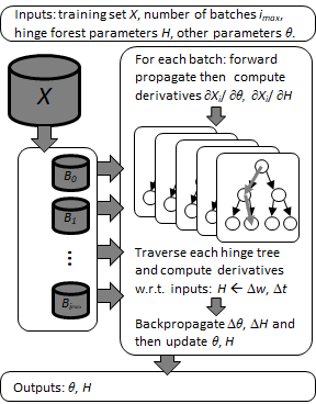
Figure 1: Illustration of random hinge forest backpropagation from algorithm 2.

Algorithm 2 TrainGraphContainingHingeForest

  Input: training set $X=\{\mathbf{x}_{n},y_{n}\}_{n=1}^{N}$, computation graph $g(\mathbf{x};H,\theta)$, batch size $N_{B}$, learning rate $\eta$, max number of gradient steps $i_{\max}$, initial depth $D$ random hinge forest parameters $H=\{(\mathbf{f}_{m},\mathbf{w}_{m},\mathbf{t}_{m})\}_{m=1}^{M}$, initial other parameters $\theta$ {Disclaimer: This is not a realistic procedure for stochastic gradient descent with backpropagation. The derivative calculation is decoupled from the other parameters to demonstrate how random hinge forest learns.}

  Output: learned parameters $H,\theta$

  for $i=0$ to $i_{\max}-1$ do

     Draw mini batch $B\subseteq X$

     Forward propagate $\quad L=\frac{1}{N_{B}}\sum_{(\mathbf{x},y)\in B}\mathcal{L}(g(\mathbf{x};H,\theta),y)$

     Compute derivatives w.r.t. to inputs for $\theta$ {Compute derivatives w.r.t. inputs for $H$}

     for $m=0$ to $M-1$ do

        Set $\Delta\mathbf{w}_{m}=\mathbf{0},\ \Delta\mathbf{t}_{m}=\mathbf{0}$

        for $j=0$ to $N_{B}-1$ do

           Set $\mathbf{z}=\text{input}_{j}$

           Compute $(\ell,r^{*},v^{*})$ = HingeTreeTraversal($D,\mathbf{z},\mathbf{t}_{m},\mathbf{f}_{m}$)

           Set $\Delta\text{input}_{jf_{mv^{*}}}\leftarrow\Delta\text{input}_{jf_{mv^{*}}}+w_{m\ell}\text{sgn}(r^{*})$

           Set $\Delta t_{mv^{*}j}\leftarrow-w_{m\ell}\text{sgn}(r^{*})$

           Set $\Delta w_{m\ell j}\leftarrow|r^{*}|$

        end for

     end for

     Backpropagate $(\Delta\theta,\Delta\mathbf{w},\Delta\mathbf{t})=\nabla L$

     Perform gradient step $\theta\leftarrow\theta-\eta\Delta\theta$

     Perform gradient step $\mathbf{w}\leftarrow\mathbf{w}-\eta\Delta\mathbf{w},\ \mathbf{t}\leftarrow\mathbf{t}-\eta\Delta\mathbf{t}$

  end for

The derivatives (11) (12) produce extremely sparse gradients. Each training example will only result in two non-zero derivatives per tree; one for the decision threshold $t_{v^{*}}$ and one for the weight (or weight tensor) $w_{\ell}$. The consequences of sparse gradients are not explored in this work. But such sparse gradients imply that the tree can be a sluggish learner. And its backpropagated derivatives can make descendants of the computation graph also sluggish. Therefore, it is important to use a suitable mini batch size (i.e. $>1$) and advisable to use an adaptive learning rate gradient optimization algorithm. This work makes use of both AdaGrad (Duchi et al., 2011) and Adam (Kingma & Ba, 2014) for fast convergence. The gradient histories of tree thresholds, weights, and parameters of descendants of the forest will be comparatively small and both AdaGrad and Adam will provide larger learning rates for such parameters with sparse derivatives.

Algorithm 3 HingeTreeTraversal

  Input: tree depth $D$, feature vector $\mathbf{x}\in\mathbb{R}^{F}$, decision thresholds $\mathbf{t}\in\mathbb{R}^{2^{D}-1}$, feature indices $\mathbf{f}\in\{0,1,\ldots,F-1\}^{2^{D}-1}$

  Output: leaf index $\ell\in\{0,1,\ldots,2^{D}-1\}$, signed margin $r^{*}\in\mathbb{R}$, vertex index $v^{*}\in\{0,1,\ldots,2^{D}-2\}$

  Initialize $\ell=0,\ v=0,\ v^{*}=0,\ r^{*}=\mathbf{x}_{\mathbf{f}_{0}}-\mathbf{t}_{0}$

  for $i=0$ to $D-1$ do

     Set $r=\mathbf{x}_{\mathbf{f}_{v}}-\mathbf{t}_{v}$

     if $|r|<|r^{*}|$ then

        Set $r^{*}\leftarrow r,\ v^{*}\leftarrow v$

     end if

     Set $\ell\leftarrow 2\ell+I(r>0)$

     Set $v\leftarrow 2v+I(r>0)+1$

  end for

5 Experiments

Two different sets of experiments were conducted to test and compare random hinge forest and ferns. The first set is run on several generic UCI (Lichman, 2013) data sets to show that both of the proposed solutions can generalize for a variety of learning tasks ranging from relatively small to large. We test configurations that vary the numbers of trees from $\{1,10,50,100\}$ and the tree depths from $\{1,3,5,7,10\}$. The best configuration is reported, and we compare against random forest (Breiman, 2001), configured to $100$ depth $10$ trees. The data sets used in the UCI experiments are summarized in Table 1 and Figure 2(a) depicts the network architecture used. All UCI experiments used AdaGrad (Duchi et al., 2011) with a single dataset-specific learning rate over all configurations.

The second set of experiments compares random hinge forest and ferns to (Kontschieder et al., 2015; Schulter et al., 2013) on the letter (Lichman, 2013), USPS (Hull, 1994), and MNIST (LeCun et al., 1998) data sets. Following the experiments of (Kontschieder et al., 2015; Schulter et al., 2013), the tree number and depth were limited to $100$ and $10$ respectively. The data sets, experiment parameters and architectures used in this experiment are summarized in Table 3 and Figures 2(b) and 2(c). Experiments used the Adam (Kingma & Ba, 2014) optimizer with $\beta_{1}=0.9$, $\beta_{2}=0.999$, and $\eta=0.005$. In contrast to the UCI experiments, these experiments report the best test error over model states since (Kontschieder et al., 2015) does not describe the use of validation sets. Lastly, to maximize our performance over MNIST, we report results for $1000$ trees/ferns.

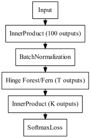
(a) Architecture used for UCI data.

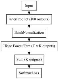
(b) Architecture used for letter and USPS.

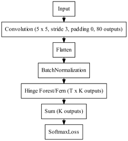
(c) Architecture used for MNIST.

Figure 2: Architectures used for results reported in this work. Here $T$ denotes the number of trees, $K$ denotes the number of class labels. The abalone regression experiment uses $\ell_{2}$ loss instead of the SoftmaxLoss.

Unlike the work of (Kontschieder et al., 2015), random hinge forest does not have learnable representations built into decision nodes. Instead, random hinge forest relies on other layers to produce a pool of learnable feature representations. For both sets of experiments, except for MNIST, we use a pool of $100$ inner product features that are randomly assigned to random hinge forest decision nodes. For MNIST, we use a single layer of $80$ $5\times 5$ convolutions with stride $3$ and no padding, which are then flattened before also being randomly assigned to decision nodes.

Table 1: UCI data set properties. All data sets had given test sets except for iris. Training sets were randomly shuffled and a small portion was kept for validation (and also testing for iris).

Data Set	Training	Validation	Testing	Dimension	Classes/Range
iris	50	50	50	3	3
abalone	2089	1044	1044	8	3
abalone regression	2089	1044	1044	8	$[1,29]$
human activity	5514	1838	2947	561	6
madelon	1500	500	600	500	2
poker	18757	6253	1000000	10	10

Both sets of experiments evaluated results over $10$ runs and the testing performances were averaged. The exception is iris, which does not possess a test set. Instead, iris was shuffled $5$ times and partitioned into $3$ folds, each used in turn as a training, validation, or test fold, totaling $15$ runs per configuration.

All experiments were conducted using an in-house and publicly available cross-platform C++14 framework (bleak). Random hinge forest should also be easily portable to other deep learning frameworks, such as Caffe. All experiments were conducted each using 1 CPU on a Windows 10 workstation running with an Intel Core i7-5930K (3.5 GHz) processor and 32 GB of RAM.

6 Results

The results of the UCI experiments are summarized in Table 2. In the three experiments involving, abalone, abalone regression and human activity, the optimal random hinge forest and ferns configuration amounted to depth 1 hinge trees/ferns, or stumps. This makes reported errors for the two identical owing to the fact that depth 1 ferns and forests are identical learning machines. Importantly, for $5$ out of $6$ experiments, random hinge forest and ferns outperform random forest. On the madelon data set, however, random forest outperformed random hinge forest and ferns by a substantial $11.5\%$. This failure is discussed in Section 7.

The second set of experiments is summarized in Table 3. random hinge forest and ferns both outperform alternating decision forest and neural decision forest on letter, while random hinge forest is only slightly better than alternating decision forest on USPS but worse than neural decision forest. Random hinge forest and ferns are similar in performance to neural decision forest on MNIST although worse than alternating decision forest.

To test the limits of random hinge forest and ferns, we tested each using $1000$ depth $10$ trees/ferns on MNIST, reducing the error to $1.81\ (0.10)$ and $1.90\ (0.06)$, respectively. This greatly outperforms alternating decision forest and neural decision forest. Importantly, despite the large number of trees, it only took $\approx 3.5$ and $\approx 3$ hours to train $1000$-tree/fern random hinge forest and ferns, respectively, over $40000$ mini batches. All other parameters were kept the same. We also experimented with two nested convolutions and random hinge forest stacking, but performance did not exceed that reported for $1000$ trees/ferns.

Lastly, Figure 3 illustrates the effects of varying tree depths and numbers of trees for both random hinge forest and ferns. These plots were each generated from the first run of the UCI madelon data set over tree depths $\{1,5,10\}$ and the first run of the MNIST data set over the number of trees $\{100,1000\}$.

Table 2: Test errors or $R^{2}$ of the best performing models over number of trees $\{1,10,50,100\}$ and depths $\{1,3,5,7,10\}$ compared to Random Forest on UCI data. The best configuration is expressed as $\text{\# trees}/\text{\# depth}$ and test error is reported as misclassification rate (standard deviation). The best performance for each data set is presented in bold.

Data Set	Hinge Forest Test	Config.	Hinge Fern Test	Config.	Random Forest
iris	$\mathbf{2.13}\ (2.66)$	10/5	$2.27\ (2.25)$	10/5	$4.13\ (2.33)$
abalone	$\mathbf{34.4}\ (0.56)$	50/1	$\mathbf{34.4}\ (0.56)$	50/1	$34.8\ (0.40)$
abalone regression ($R^{2}$)	$\mathbf{0.57}\ (0.07)$	100/1	$\mathbf{0.57}\ (0.07)$	100/1	$0.54\ (0.01)$
human activity	$\mathbf{5.52}\ (0.51)$	50/1	$\mathbf{5.52}\ (0.51)$	50/1	$8.23\ (0.50)$
madelon	$40.8\ (1.60)$	10/3	$40.8\ (1.41)$	50/7	$\mathbf{29.3}\ (1.13)$
poker	$\mathbf{32.6}\ (4.80)$	50/3	$33.9\ (4.70)$	100/3	$40.4\ (0.18)$

Table 3: Data set sizes, tree inputs, and classification error of random hinge forest, ferns, alternating decision forest (Schulter et al., 2013) and neural decision forest (Kontschieder et al., 2015). All features for the random hinge forest/ferns were simultaneously learned via backpropagation as part of random hinge forest/fern training. Test errors are expressed as average misclassification rate (standard deviation). The best performance for each data set is presented in bold.

	Letter (Lichman, 2013)	USPS (Hull, 1994)	MNIST (LeCun et al., 1998)
Training	16000	7291	60000
Testing	4000	2007	10000
Classes	26	10	10
Dimension	16	$16\times 16$	$28\times 28$
Features	100 inner product	100 inner product	80 $5\times 5$ convolutions
Batch Size	53	29	53
Random Hinge Forest	$\mathbf{2.56}\ (0.11)$	$5.53\ (0.15)$	$2.79\ (0.11)$
Random Hinge Ferns	$2.78\ (0.12)$	$5.64\ (0.24)$	$2.85\ (0.13)$
Alternating Decision Forest	$3.42\ (0.17)$	$5.59\ (0.16)$	$\mathbf{2.71}\ (0.10)$
Neural Decision Forest	$2.92\ (0.17)$	$\mathbf{5.01}\ (0.24)$	$2.8\ (0.12)$

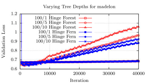
(a) Validation loss evolution for madelon.

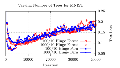
(b) Test loss evolution for MNIST.

Figure 3: Validation/Test loss behaviors for varying tree depth 3(a) and varying numbers of trees 3(b). Deeper trees and more trees both have the potential to generalize better, but can also severely overfit resulting in increasing validation/test losses over training iteration. Legends are to be interpreted as # trees / # depth.

7 Discussion

The UCI experiments demonstrate that random hinge forest and ferns can perform well on both relatively large and tiny data sets for a variety of learning tasks not usually attributed to differentiable learning. While not tabulated, the results over the varying numbers of trees and tree depths were often similar. In all but one case, both random hinge forest and ferns outperform random forest. The exception, i.e., the madelon (Lichman, 2013) dataset, is a synthetic binary classification problem generated from a number of Gaussian distributions as well as an abundance of useless noise features with a few other complexities added. We tried a number of different configurations, quantity of learnable features, weight decay, using Adam instead of AdaGrad, and feature selection, but we consistently obtained misclassification rates of $\approx 40.0$. In all tests, except for when using weight decay, the random hinge forest typically overfit the training data to perfection. Therefore, the most likely cause of poor performance is that inner product features are not suitable learnable features for the madelon data set. Where trees in random forest can deliberately choose split features as they grow, ignoring ones that do not prove useful to their task, hinge trees are assigned randomized learnable split features. Although these may be adjusted to fit its own randomized decision structure, they cannot be rejected. A hypothetical sparse learnable inner product feature might overcome this limitation as this would behave like the decisions used in trees of random forest. We leave this to future work.

The second set of experiments attempts to respect the constraints imposed on alternating decision forest and neural decision forest, where we limit ourselves to no more than $100$ depth $10$ trees. Importantly, while alternating decision forest are flexible enough to be employed with any loss function and neural decision forest can be incorporated within an arbitrary differentiable computation graph, random hinge forest and ferns are the first learnable decision tree machinery that can do both. In terms of performance, random hinge forest and ferns are comparable to alternating decision forest and neural decision forest. Our methods perform best on letter, second to neural decision forest on USPS, and second to alternating decision forest on MNSIT. Though, random hinge forest probably has the same performance as neural decision forest on MNIST. Noteworthy is that we maintain competitive performance on these three data sets with only a pool of $100$ learnable features for letter and USPS and $80$ learnable convolution kernels that produce $5120$ features when flattened on MNIST. By comparison, neural decision forest have a learnable innerproduct decision at every vertex of every decision tree, often resulting in many more parameters than random hinge forest. For instance, neural decision forest uses $\approx 10\times$ more parameters for USPS and about $\approx 17\times$ more parameters for MNIST. random hinge forest use about $10\%$ more parameters than neural decision forest for letter. Additionally, the competitive ferns have approximately half as many parameters as random hinge forest.

Also, random hinge forest and ferns do not require such large mini batch sizes as used for neural decision forest, e.g. 1000 for the MNIST dataset (Kontschieder et al., 2015). The large mini batch size for the latter is likely needed for the prediction node optimization when training, as the histograms have to be adequately populated. However, random hinge forest can predict arbitrary weight vectors and are not limited to probability vectors and average leaf purity over the trees. Thus, random hinge forest can train with small batch sizes which, in combination with its logarithmic gradient calculation complexity, results in faster training and convergence. This efficient formulation, however, does limit random hinge forest to piecewise linear behavior while neural decision forest are naturally non-linear owing to its use of sigmoid decision functions and multiple leaves in prediction. These efficiencies translate into practical improvements. For example, if not for this efficiency, it would be prohibitively expensive to train $1000$ depth $10$ trees with learnable features on a single CPU. With OpenMP/C++11 threads and/or GPU acceleration, this could even be substantially faster.

8 Conclusion

Random hinge forest and ferns are efficient end-to-end learning machines that can be used to solve a variety of learning tasks on both relatively small and large data sets. Their ability to coexist in backpropagating computation graphs enables them to minimize a global loss function, be connected with any other differentiable component, and exploit learnable feature representations not afforded to the original random forest. This flexibility also comes with a robustness that can tolerate a variety of configurations and parameter initializations. We hope that random hinge forest can complement current deep learning machinery and maybe provide a simple means for new or experienced machine learning practitioners to develop and explore their own network architectures.

References

- Amit & Geman (1997) Amit, Yali and Geman, Donald. Shape quantization and recognition with randomized trees. Neural computation, 9(7):1545–1588, 1997.
- Breiman (2001) Breiman, Leo. Random forests. Machine learning, 45(1):5–32, 2001.
- Criminisi et al. (2010) Criminisi, Antonio, Shotton, Jamie, Robertson, Duncan, and Konukoglu, Ender. Regression forests for efficient anatomy detection and localization in ct studies. In International MICCAI Workshop on Medical Computer Vision, pp. 106–117. Springer, 2010.
- Duchi et al. (2011) Duchi, John, Hazan, Elad, and Singer, Yoram. Adaptive subgradient methods for online learning and stochastic optimization. Journal of Machine Learning Research, 12(Jul):2121–2159, 2011.
- Friedman (1991) Friedman, Jerome H. Multivariate adaptive regression splines. The annals of statistics, pp. 1–67, 1991.
- Friedman (2001) Friedman, Jerome H. Greedy function approximation: a gradient boosting machine. Annals of statistics, pp. 1189–1232, 2001.
- Gall & Lempitsky (2013) Gall, Juergen and Lempitsky, Victor. Class-specific hough forests for object detection. In Decision forests for computer vision and medical image analysis, pp. 143–157. Springer, 2013.
- He et al. (2016) He, Kaiming, Zhang, Xiangyu, Ren, Shaoqing, and Sun, Jian. Deep residual learning for image recognition. In Proceedings of the IEEE conference on computer vision and pattern recognition, pp. 770–778, 2016.
- Hull (1994) Hull, Jonathan J. A database for handwritten text recognition research. IEEE Transactions on pattern analysis and machine intelligence, 16(5):550–554, 1994.
- Ioffe & Szegedy (2015) Ioffe, Sergey and Szegedy, Christian. Batch normalization: Accelerating deep network training by reducing internal covariate shift. In International conference on machine learning, pp. 448–456, 2015.
- Kingma & Ba (2014) Kingma, Diederik P and Ba, Jimmy. Adam: A method for stochastic optimization. arXiv preprint arXiv:1412.6980, 2014.
- Kontschieder et al. (2015) Kontschieder, Peter, Fiterau, Madalina, Criminisi, Antonio, and Bulo, Samuel Rota. Deep neural decision forests. In Computer Vision (ICCV), 2015 IEEE International Conference on, pp. 1467–1475. IEEE, 2015.
- Krizhevsky et al. (2012) Krizhevsky, Alex, Sutskever, Ilya, and Hinton, Geoffrey E. Imagenet classification with deep convolutional neural networks. In Advances in neural information processing systems, pp. 1097–1105, 2012.
- LeCun et al. (1998) LeCun, Yann, Bottou, Léon, Bengio, Yoshua, and Haffner, Patrick. Gradient-based learning applied to document recognition. Proceedings of the IEEE, 86(11):2278–2324, 1998.
- Lichman (2013) Lichman, M. UCI machine learning repository, 2013. URL http://archive.ics.uci.edu/ml.
- Ozuysal et al. (2010) Ozuysal, Mustafa, Calonder, Michael, Lepetit, Vincent, and Fua, Pascal. Fast keypoint recognition using random ferns. IEEE transactions on pattern analysis and machine intelligence, 32(3):448–461, 2010.
- Ronneberger et al. (2015) Ronneberger, Olaf, Fischer, Philipp, and Brox, Thomas. U-net: Convolutional networks for biomedical image segmentation. In International Conference on Medical image computing and computer-assisted intervention, pp. 234–241. Springer, 2015.
- Schulter et al. (2013) Schulter, Samuel, Wohlhart, Paul, Leistner, Christian, Saffari, Amir, Roth, Peter M, and Bischof, Horst. Alternating decision forests. In Computer Vision and Pattern Recognition (CVPR), 2013 IEEE Conference on, pp. 508–515. IEEE, 2013.
- Simonyan & Zisserman (2014) Simonyan, Karen and Zisserman, Andrew. Very deep convolutional networks for large-scale image recognition. arXiv preprint arXiv:1409.1556, 2014.
- Suárez & Lutsko (1999) Suárez, Alberto and Lutsko, James F. Globally optimal fuzzy decision trees for classification and regression. IEEE Transactions on Pattern Analysis and Machine Intelligence, 21(12):1297–1311, 1999.