QRkit: Sparse, Composable QR Decompositions for
Efficient and Stable Solutions to Problems in Computer Vision

Abstract

Embedded computer vision applications increasingly require the speed and power benefits of single-precision (32 bit) floating point. However, applications which make use of Levenberg-like optimization can lose significant accuracy when reducing to single precision, sometimes unrecoverably so. This accuracy can be regained using solvers based on QR rather than Cholesky decomposition, but the absence of sparse QR solvers for common sparsity patterns found in computer vision means that many applications cannot benefit. We introduce an open-source suite of solvers for Eigen, which efficiently compute the QR decomposition for matrices with some common sparsity patterns (block diagonal, horizontal and vertical concatenation, and banded). For problems with very particular sparsity structures, these elements can be composed together in ‘kit’ form, hence the name QRkit. We apply our methods to several computer vision problems, showing competitive performance and suitability especially in single precision arithmetic.

1 Introduction

Computer vision applications are increasingly required to run on low-power architectures, where single precision floating point is significantly more efficient than double [3, 25, 34]. However, where such applications depend on Levenberg-like solvers (e.g. bundle adjustment [1, 40, 41], SLAM [8], 3D reconstruction [39], surface fitting [9, 37, 38]), single precision operation can negatively impact accuracy, and may therefore require more solver iterations, or may simply never be accurate enough.

In this paper, we identify an important contributor to such inaccuracy: the use of Cholesky decomposition to solve equations of the form

$$(J^{\top}J+\lambda D^{2})p=J^{\top}b$$ (1)

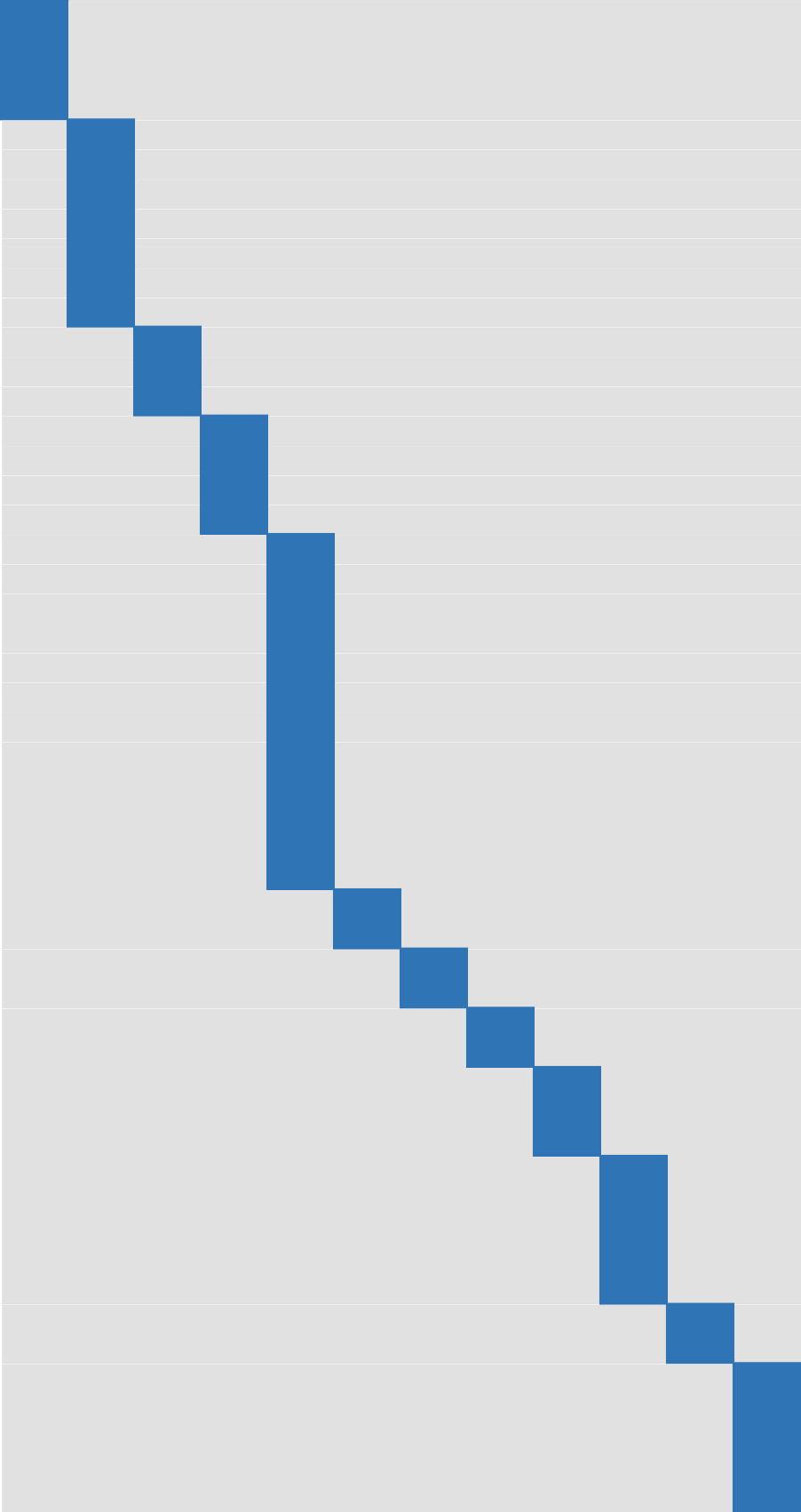
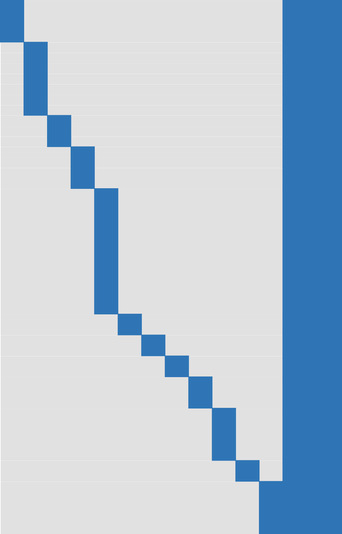
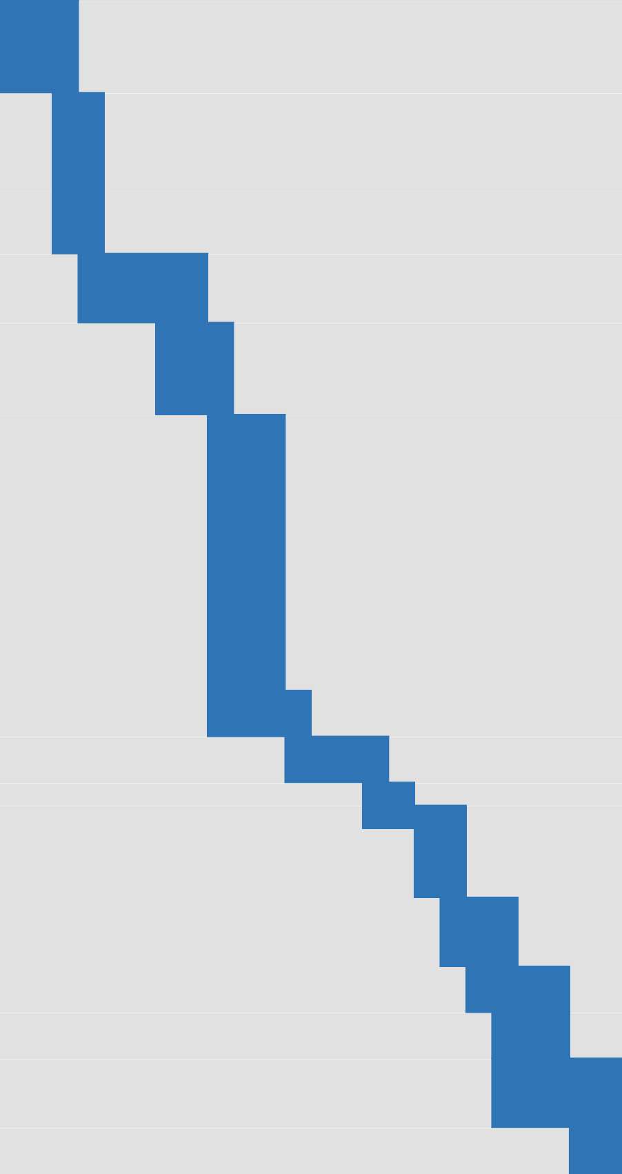
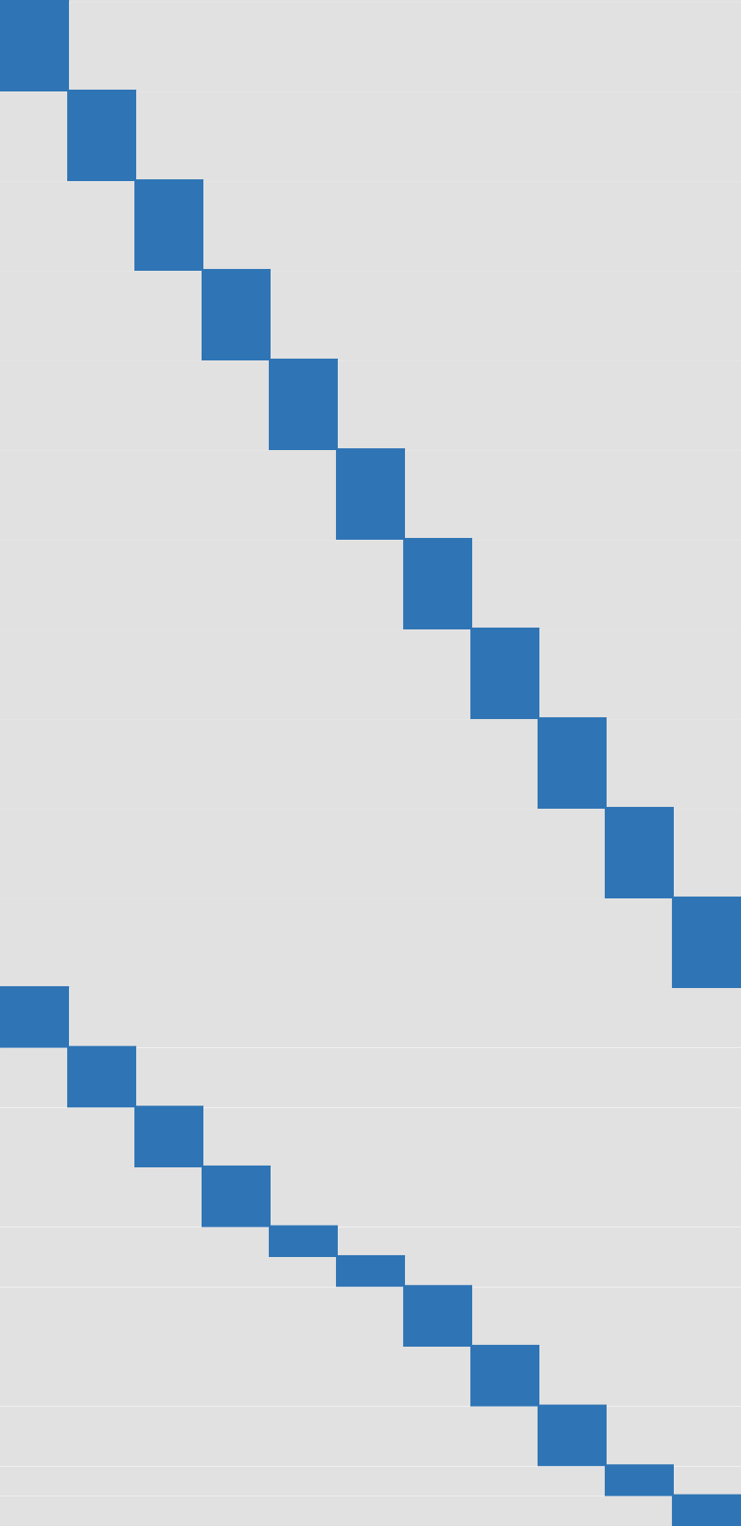
Figure 1: Sparsity patterns. (a) Block diagonal, (b) Horizontal concatenation of [Easy, Dense], including Angular, (c) Banded, (d) Row-permuted banded (includes vertical concatenation of some easier cases).

for unknown vector $p$ given: vector $b$, diagonal matrix $D$, and matrix $J$. Typically $J$ is rectangular and sparse with particular sparsity structures (some are illustrated in Figure 1) that can be exploited in Cholesky decomposition. However, $J^{\top}J$ has a condition number which is the square of $J$, which can adversely affect numerical precision and robustness.

The squaring can be avoided by solving the equivalent least squares system

$$\begin{pmatrix}J\\ \lambda^{\frac{1}{2}}D\end{pmatrix}p=\begin{pmatrix}b\\ 0\end{pmatrix}$$ (2)

using QR decomposition, as is in the classic Levenberg–Marquardt implementation of Moré [31]. In the dense case, this is typically twice as many floating-point operations per iteration than the Cholesky solution, but the reduction in iteration count for a given accuracy can be significant.

In the sparse case, the story is less rosy. There are general-purpose sparse QR implementations, e.g. the SPQR routines in SuiteSparse [12], which make the method competitive with Cholesky for many problems. However, there are no libraries which offer QR solvers which can exploit the particular sparsity structures in typical computer vision problems, so the QR method is unusably slow, even though it may be ultimately more accurate.

The contribution of this paper is to collate from the numerical analysis literature a small collection of special-purpose solvers, with the property that they can be composed in ‘kit’ form to easily build fast solvers for a wide range of computer vision applications. The wider contribution is to allow the use of efficient single-precision optimization routines without catastrophic loss of accuracy.

We structure the paper by first reviewing the properties and use of the QR decomposition. Second, we explain our strategy for building efficient solvers, and present a collection of such solvers. Third, we show results on a range of computer vision benchmarks, for QR-based and Cholesky-based algorithms in both single and double precision.

Notation

Let $\mathbf{e}_{i}$ denote the $i$th column of the $n\times n$ identity matrix. The Kronecker product $A\otimes B$ puts a scaled copy of $B$ at every entry in $A$, for example if $B$ is $p\times q$, then $\mathbf{e}_{i}\otimes B$ is a matrix of size $np\times q$ with structure $[0_{(i-1)p\times q};B;0_{(n-i+1)p\times q}]$. To flag where a QR decomposition is computed numerically, we write $QR={\tt qr}(A)$.

2 Background: QR decomposition

Given a matrix $A$, the QR decomposition finds matrices $Q$ and $R$ such that $Q$ is orthonormal ($Q^{\top}Q=I$), $R$ is upper triangular, and $A=QR$. We generally deal with matrices $A$ in ‘portrait’ orientation, so $m>n$, and with the ‘economy-size’ decomposition where $Q$ has size $m\times n$ and $R$ is $n\times n$. However, we will need access to the orthogonal complement of $Q$, written $Q^{\perp}$, size $(n-m)\times n$, and to the ‘full size’ matrices

$$\mathbf{Q}=\left[Q~{}\middle|~{}Q^{\perp}\right],\qquad{\mathbf{R}}=\left[\begin{matrix}R\\ 0\end{matrix}\right]$$ (3)

which will often be too large to store explicitly. Therefore, as is common in QR decomposition routines, we may store not $Q$ itself, but some C++ object ${\tt Q}$ which behaves like $Q$; that is, it implements the operations of matrix multiplication. Then, to look at $Q$ itself (for example, when debugging small problems), we multiply ${\tt Q}$ by a representation of the $n\times n$ identity matrix.

The rich history of QR decomposition dates back to the early 1950s, when it was introduced independently by Francis [15, 16] and Kublanovskaya [24], who proposed the use of QR decomposition as a solution to the eigenvalue problem. QR decomposition can be carried out using Gram-Schmidt orthogonalization [5], Givens rotations [18] or Householder reflections [23]; all the approaches were summarized later by Gander [17]. The method became popular at the time, exploited by many showing its use for singular value decomposition [19] and solution to least squares problems [19].

Many important methods are based on Householder matrices of the form $H=I-2vv^{T}$, where $v$ is a Householder vector [23] having unit 2-norm. Householder matrices are orthogonal and can be used to zero-out selected columns of a matrix. Householder QR decomposition of $n\times m$ matrix $A$ can be therefore expressed as multiplication by sequence of Householder matrices $H_{m-1},\cdots,H_{0}$, i.e.

$$\mathbf{R}=H_{m-1}\cdots H_{0}A=\mathbf{Q}^{T}A,$$ (4)

where each $H_{k},k\in\{0,\cdots,m-1\}$ is of size $m\times m$.

Bischof et al. [4] and Scheiber et al. [35] introduced the blocked versions of Householder transformation, in order to reduce the burden of inefficient matrix-vector operations on the supercomputing architectures of the time. Given matrices $B,C\in\mathbb{R}^{n\times r}$ and $B_{1},C_{1}\in\mathbb{R}^{r\times r}$ we want to find an orthogonal $\mathbf{Q}\in\mathbb{R}^{n\times n}$ such that

$$B=\left[\begin{matrix}B_{1}\\ B_{2}\end{matrix}\right],\qquad\mathbf{Q}^{T}B=C=\left[\begin{matrix}C_{1}\\ 0\end{matrix}\right].$$ (5)

Using the ‘WY’ representation by Bischof et al. [4], the solution to the problem is represented as

$$\mathbf{Q}=I+WY^{T},\qquad W,Y\in\mathbb{R}^{n\times r},$$ (6)

where $Y$ is lower trapezoidal, i.e., $y_{ij}=0\mathrm{~{}if~{}}i<j$. The submatrix $C_{1}$ is upper triangular and $\mathbf{Q}$ is a rank-1 correction to the identity, and so it can be regarded as a generalization of the Householder matrix [36].

Schreiber et al. [36] show how to modify the WY representation so that only $nr$ storage is required. The matrix $\mathbf{Q}$ from (6) can be expressed as

$$\mathbf{Q}=I+YTY^{T},\qquad Y\in\mathbb{R}^{n\times r},T\in\mathbb{R}^{r\times r},$$ (7)

where $Y$ is lower trapezoidal and $T$ upper triangular. This is usually referred to as a compressed WY representation. For details on computation of blocked Householder representations, we refer the reader to [36].

Later interest in parallel computing motivated researchers to explore parallel QR decomposition algorithms [11, 32], in a thread that continues as a subject of active research [7, 14, 21].

Alongside other methods, QR decomposition has been implemented as a part of the LAPACK package [2] in 1990 and much more recently Davis [12] developed a multifrontal rank-revealing version (SPQR) in the SuiteSparse library.

A very appealing application of QR factorization arises in the field of numerical optimization, in particular solving non-linear least squares problems. It is of particular interest in use together with the Levenberg [27] Marquardt [29] algorithm. This is a popular variant of the Gauss–Newton method for finding the minimum of a function $F(x)$ represented as a sum of squares of generally nonlinear functions

$$F(x)=\|f(x)\|^{2}=\frac{1}{2}\sum_{i=1}^{m}[f_{i}(x)^{2}],$$ (8)

from which comes the above-mentioned instance of (1), with the matrix $J$ being the Jacobian of $f:\mathbb{R}^{n}\mapsto\mathbb{R}^{m}$, and the vector $b=-f(x)$.

There are various strategies for updating the damping parameter $\lambda$. Moré’s implementation employs a trust-region method proposed by Hebden [22].

To reduce the number of matrix factorizations, Lourakis et al. [28] presented an alternative approach to updating the damping factor, better suited for computer vision latent variable problems such as bundle adjustment. Instead of seeking a nearly exact solution for $\lambda$ using Newton’s algorithm in a trust-region framework (as proposed by Conn et al. [10] and Moré [31]), it directly controls the damping factor $\lambda$ with a line-search algorithm [28].

3 Building sparse QR solvers

The general strategy to build efficient solvers [6, 14] is to express the matrix $A$ as some combination of smaller matrices $A_{1..K}$, for whose shape it is easy (i.e. efficient) to store and compute the QR decomposition. Then manipulations of these easy QRs leads to the decomposition of $A$. The composition of these solvers in code is a compile-time declaration in terms of the data types of component solvers. For example, a matrix with four blocks (see Figure 2(a)) might have the top-left block defined as block diagonal, with $p$ component blocks of size $2\times 3$, the top-right as general dense of size $p\times q$, and the bottom-left block expressed as ‘block-banded’. Consulting Figure 2(a), the best way to encode this is as a vertical concatenation of $A_{1}$ and $A_{2}$ followed by horizontal concatenation with $A_{3}$ and a $0$ block, expressed as

$$\left[\left[\begin{matrix}A_{1}\\ A_{2}\end{matrix}\right]~{}\middle|~{}\left[\begin{matrix}A_{3}\\ 0\end{matrix}\right]\right].$$ (9)

4 QRkit

QRkit supports efficient factorization of the sparsity patterns and their compositions that will be described in the following sections.

4.1 Block diagonal

If the matrix $A$ is block diagonal, i.e. $A=\mathtt{blkdiag}(A_{1},...,A_{K})$, then to find matrices $Q,R$ as above, we define $Q_{k}R_{k}={\tt qr}(A_{k})$ for all $k$. Observe that $\mathbf{e}_{j}\otimes Q_{j}$ is orthogonal to $\mathbf{e}_{k}\otimes Q_{k}$ for all $k\neq j$, because the nonzeros don’t overlap, so we can simply write $Q=\mathtt{blkdiag}(Q_{1},...,Q_{K})$, and $R=\mathtt{blkdiag}(R_{1},...,R_{K})$. The class BlockDiagonalQR is templated over the solver type BlockSolver of the individual blocks. For example

 BlockDiagonalQR<DenseQR> slvr;

For the simple block diagonal case, matrix $Q$ is very sparse and can therefore be formed explicitly as well as using a vector of BlockSolvers. The upper triangular factor $R$ exhibits strong sparsity as well and all of its elements are close to the matrix main diagonal. An example of QR factorization of a block diagonal matrix is shown Figure 2(b) and 2(c).

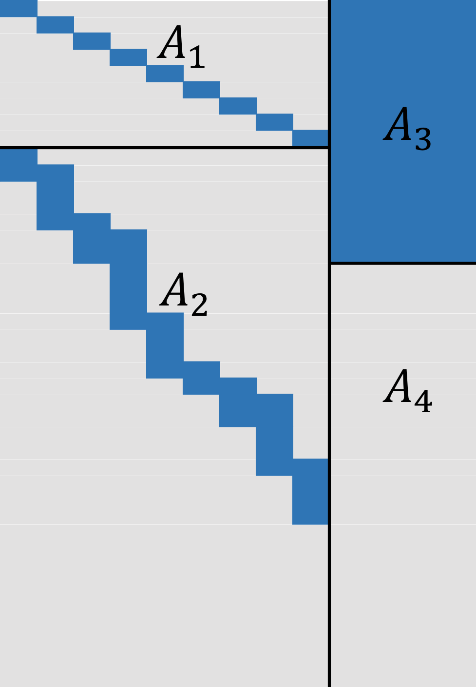
(a) $A$

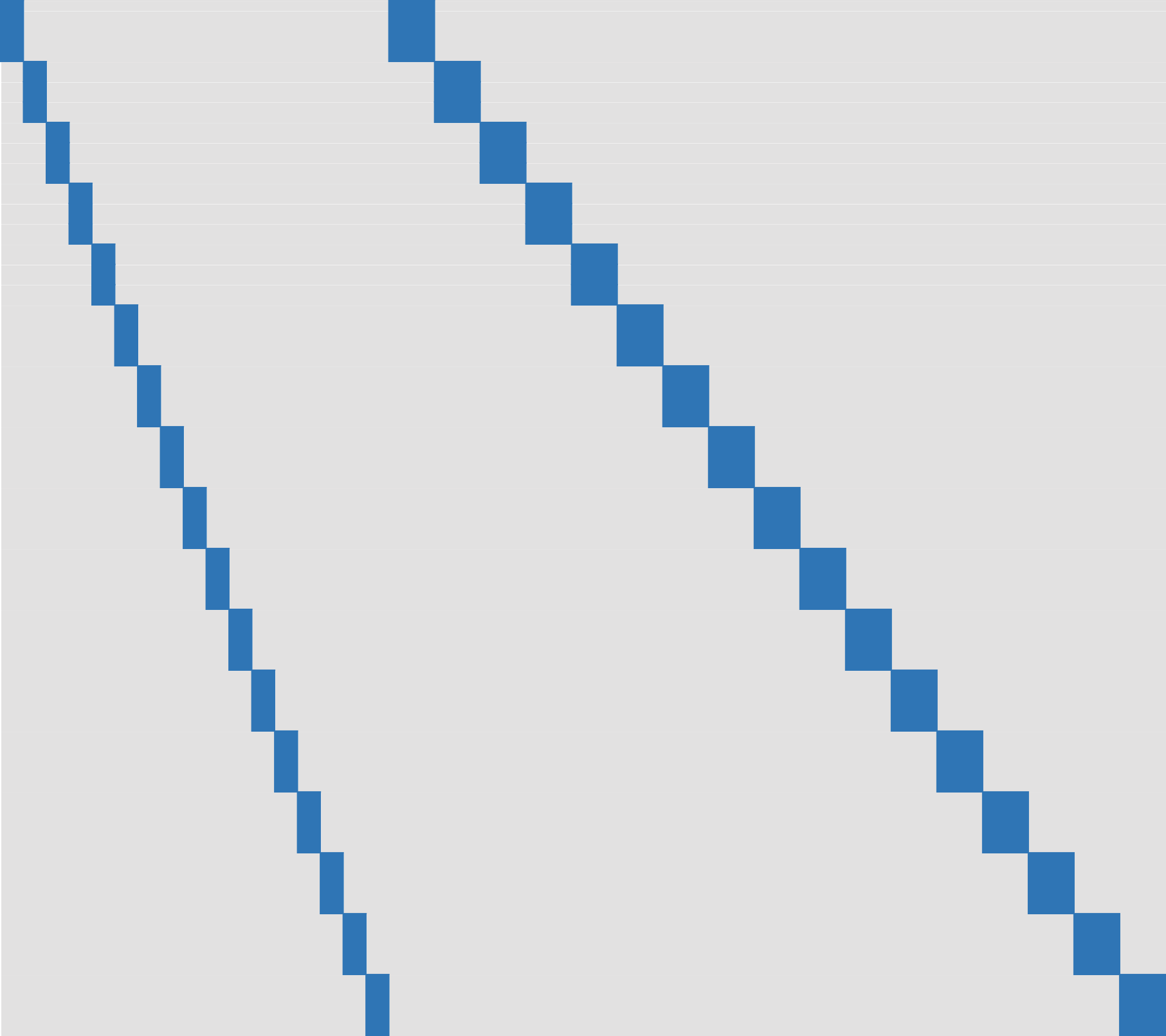
(b) $\mathbf{Q}$

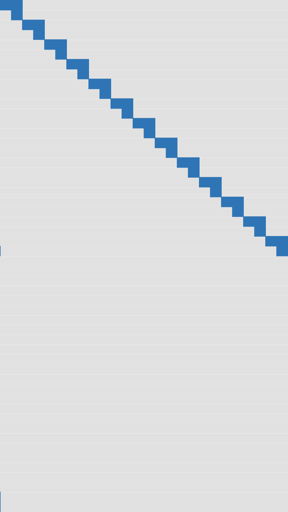
(c) $R$

Figure 2: (a) An example of favorable sparsity patterns in different blocks of matrix $A$. (b-c) Typical sparsity of QR decomposition of a block diagonal matrix (e.g. block $A_{1}$ in $A$). In $\mathbf{Q}$, the left diagonal forms $Q$ and the right diagonal $Q^{\perp}$, and $\mathbf{Q}=\left[Q~{}\middle|~{}Q^{\perp}\right]$.

4.2 Horizontal concatenation

Horizontal concatenation of two or more matrices with different sparsity structure is a common pattern in many applications [1, 9, 38, 40, 41]. The core computational unit is the concatenation of two blocks, with matrix $A_{1}\in\mathbb{R}^{n\times m_{1}}$ and matrix $A_{2}\in\mathbb{R}^{n\times m_{2}}$:

$$A=\left[A_{1}~{}\middle|~{}A_{2}\right]$$ (10)

We assume again that $A_{1}$ has a structure which makes

$$Q_{1}R_{1}={\tt qr}(A_{1})$$

efficient to compute. Rewriting $A$ using full size $\mathbf{Q}_{1}$ gives

$$A =\left[Q_{1}R_{1}~{}\middle|~{}A_{2}\right]$$

$$=\left[\mathbf{Q}_{1}\left[\begin{matrix}R_{1}\\ 0\end{matrix}\right]~{}\middle|~{}\mathbf{Q}_{1}\mathbf{Q}_{1}^{\top}A_{2}\right]$$

$$=\mathbf{Q}_{1}\left[\left[\begin{matrix}R_{1}\\ 0\end{matrix}\right]~{}\middle|~{}\mathbf{Q}_{1}^{\top}A_{2}\right]$$

We now have the product of a unitary matrix $\mathbf{Q}_{1}$ and a matrix whose top $m_{1}$ rows are upper triangular. We now factorize the bottom $n-m_{1}$ rows of $\mathbf{Q}_{1}^{\top}A_{2}$, which, from (3), is ${Q^{\perp}_{1}}^{\top}A_{2}$.

$$Q^{\prime}R^{\prime}={\tt qr}({Q^{\perp}_{1}}^{\top}A_{2})$$ (11)

And following from above,

$$A =\mathbf{Q}_{1}\left[\left[\begin{matrix}R_{1}\\ 0\end{matrix}\right]~{}\middle|~{}\left[\begin{matrix}Q_{1}^{\top}A_{2}\\ Q^{\prime}R^{\prime}\end{matrix}\right]\right]$$

$$=\mathbf{Q}_{1}\left[\left[\begin{matrix}R_{1}\\ 0\end{matrix}\right]~{}\middle|~{}\left[\begin{matrix}I&0\\ 0&\mathbf{Q}^{\prime}\end{matrix}\right]\left[\begin{matrix}Q_{1}^{\top}A_{2}\\ R^{\prime}\\ 0\end{matrix}\right]\right]$$

$$=\mathbf{Q}_{1}\left[\begin{matrix}I&0\\ 0&\mathbf{Q}^{\prime}\end{matrix}\right]\left[\left[\begin{matrix}R_{1}\\ 0\end{matrix}\right]~{}\middle|~{}\left[\begin{matrix}Q_{1}^{\top}A_{2}\\ R^{\prime}\\ 0\end{matrix}\right]\right]$$

An implementation may form the product, or simply store $Q_{1}$ and $Q^{\prime}$ in ${\tt Q}$.

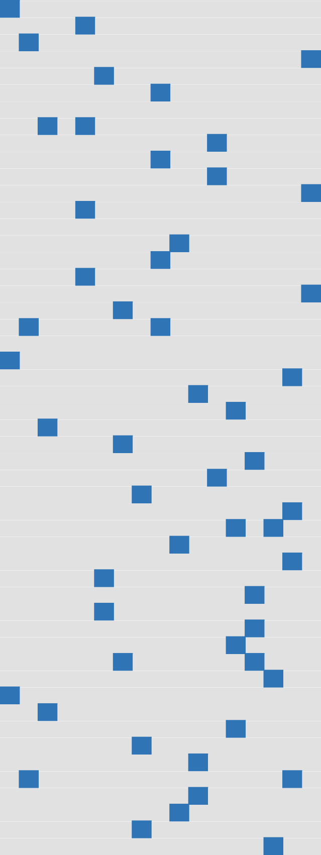
(a) $A$

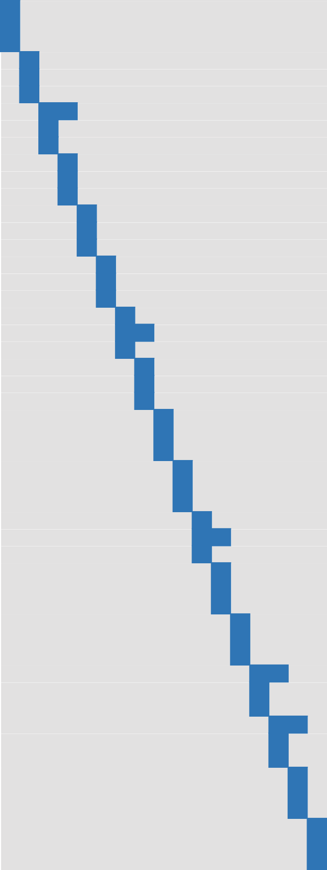
(b) $P_{r}A$

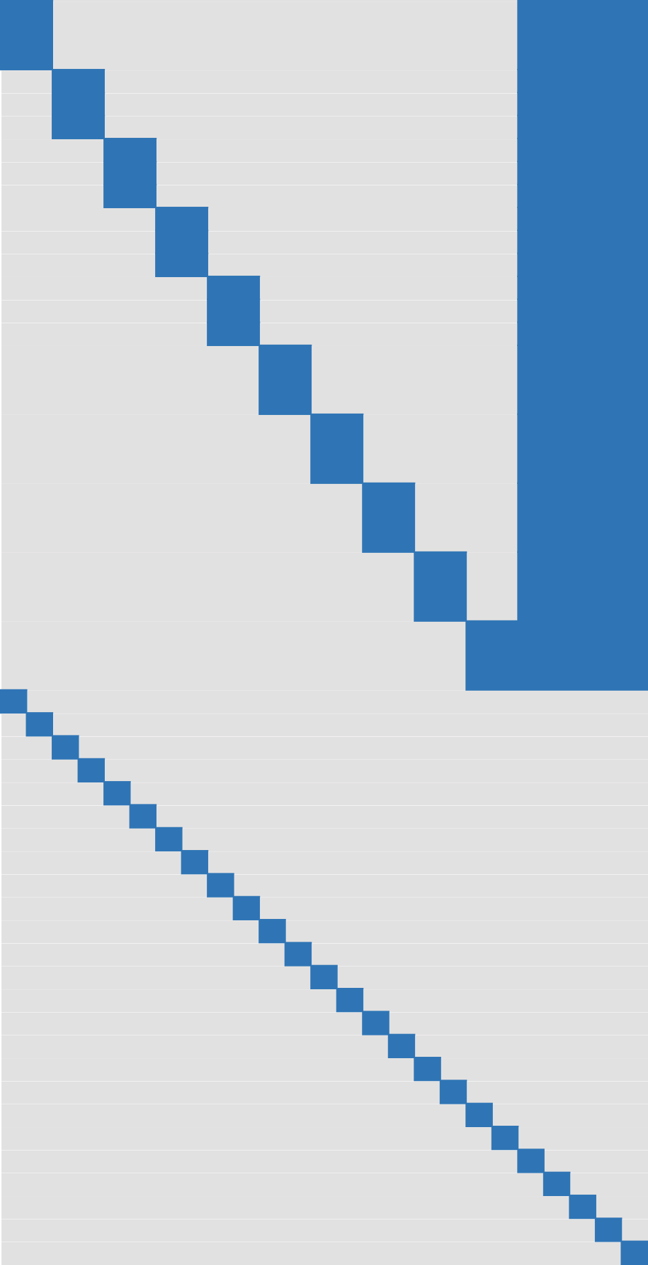
(c) $B$

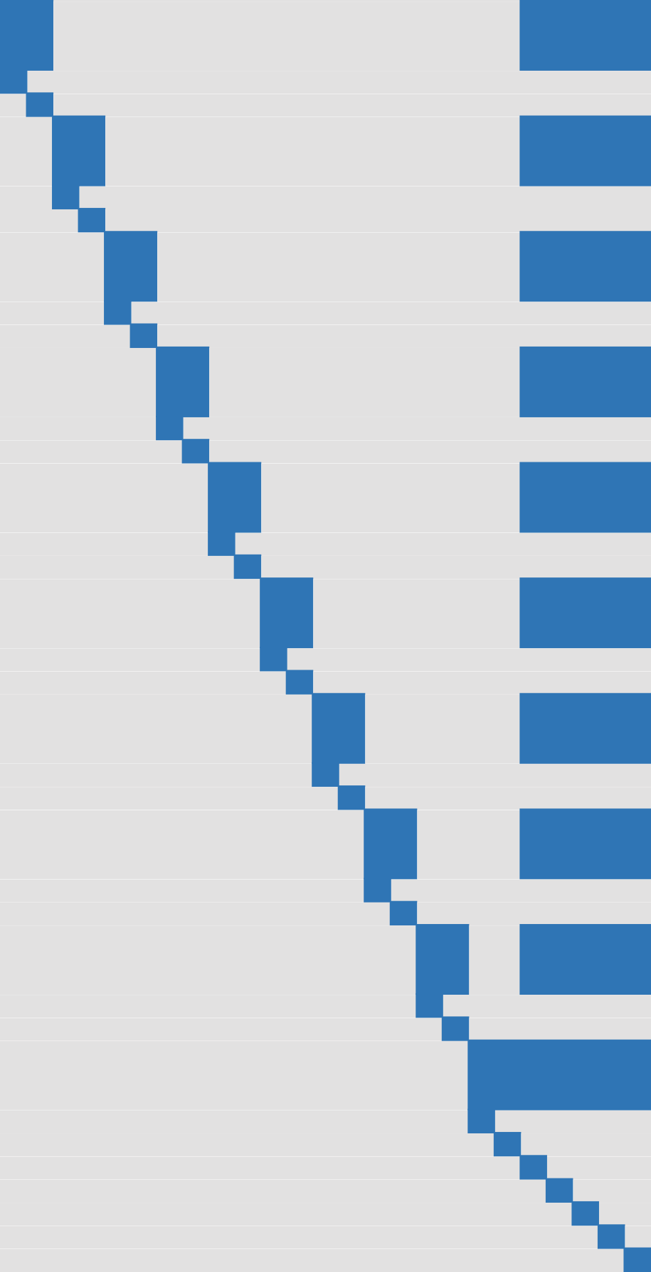
(d) $P_{r}B$

Figure 3: (a-b) Row permutation $P_{r}$ discovering banded structure in the matrix $A$. (c-d) Row permutation $P_{r}$ while solving vertical concatenation of two matrices.

4.3 Row and column permutations

A common sparsity pattern is not always obvious. This can be demonstrated by generating a block diagonal/banded matrix $A\in\mathbb{R}^{n\times m}$ and applying a random permutation $P_{r}\in\{0,1\}^{n\times n}$ to its rows (see Figure 3(a) and 3(b)). Applying this process in reverse to a sparse input matrix $A$, we can search for a row permutation $P_{r}$ that would reorder the rows in order to create an ‘As-Banded-As-Possible’ sparsity pattern [13]. The resulting matrix $A^{\prime}\in\mathbb{R}^{n\times m}$:

$$A^{\prime}=P_{r}A$$ (12)

can be factorized using our efficient solvers.

Another common technique is to permute the columns of $A$ using a permutation matrix $P_{c}\in\{0,1\}^{m\times m}$, obtaining

$$A^{\prime}=AP_{c},$$ (13)

which is often used in order to reduce fill-in during the QR decomposition.

The best practice is to combine both permutations by searching for a row-banded structure in $A$ and reducing the fill-in of the QR decomposition at the same time. The QR solver will then be performing decomposition of

$$A^{\prime}=P_{r}AP_{c}.$$ (14)

4.4 Block banded

Adding new residuals to a block-diagonal optimization problem may create overlaps between the diagonal blocks of the Jacobian and therefore break the block diagonal structure of $A$ described in Section 4.1.

Given block banded $A\in\mathbb{R}^{n\times m}$, such as $A_{2}$ from Figure 2(a), let ${\tt blk_{k}}{(A)}\in\mathbb{R}^{n_{k}\times m_{k}}$ be the $k$th block of $A$. Writing $r_{k}\in\{0,\cdots,\textit{min}(m_{k},m_{k+1})\}$ for the number of overlapping columns of blocks ${\tt blk_{k}}{(A)}$ and ${\tt blk_{k+1}}{(A)}$, we assume $r_{k}\ll m$.

Instead of performing QR factorization of the whole $A$, which would yield Householder vectors of length $n$, we can create block-wise Householder vectors of length $n_{k}+n_{k+1}$ for the $k$th block. Typically $n_{k}+n_{k+1}\ll n$, which results in both faster execution and lower memory consumption. The sparse Householder vectors can be stored as columns of a big sparse matrix as depicted in Figure 4(a).

Exploiting structural zeros in such a way allows us to perform operations on small dense blocks and sequentially combine the partial results, instead of performing operations on the large sparse matrix $A$, which would suffer from both the size of $A$ and the fact that operations for sparse matrices cannot be implemented as efficiently as the dense case.

Striving for better performance, we use the compressed WY representation of Householder QR (see Section 2 for details). Using dense blocks of size $n_{j}\times r$, we factorize $r$ columns of $A$ in the $j$th step as

$$\begin{split}A_{j+1}^{\prime}=Q_{j}^{\top}A_{j}&=(I+Y_{j}T_{j}Y_{j}^{\top})^{\top}A_{j}\\ &=A_{j}+Y_{j}(T_{j}^{\top}(Y_{j}^{\top}A_{j})),\end{split}$$ (15)

where $Y\in\mathbb{R}^{n_{j}\times r}$, $T\in\mathbb{R}^{r\times r}$ and $r<n_{j}$. Factorization of $A$ is expressed as a sequence of $K$ such economy blocked transformations in form

$$A^{\prime}=(I+Y_{k-1}T_{k-1}Y_{k-1}^{\top})^{\top}\cdots(I+Y_{0}T_{0}Y_{0}^{\top})^{\top}A,$$ (16)

where $k\in\{0,\dots,K-1\}$. It can be observed that matrix $Q$ expressed explicitly would be at least $60\%$ dense in this case. On the other hand, representing $Q$ as a series of the economy blocked transformations is extremely sparse. A pictorial example of the factorization is in Figure 4.

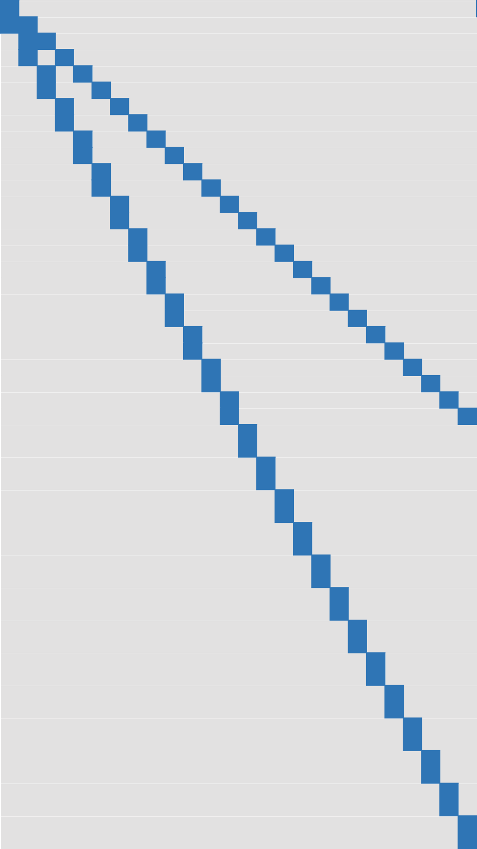
(a) Blocks Y

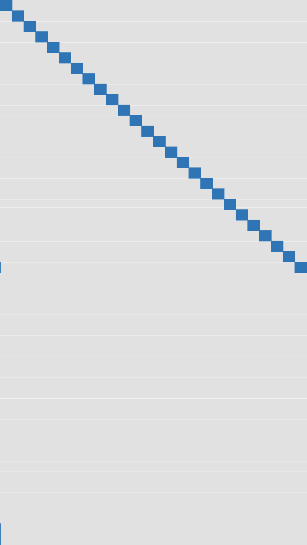
(b) Blocks T

(c) Matrix Q

(d) Matrix R

Figure 4: Sparsity patterns of the QR factorization of a block banded matrix. Matrices of blocks Y and T store, column-wise using sparse representation, the small blocks Y and T that are used to factorize several columns of the input matrix at a time.

4.5 Vertical concatenation

In general, vertical concatenation of two QR decompositions is much harder than the horizontal concatenation discussed in Section 4.2. The main unit is the two-block case, having $A_{1}\in\mathbb{R}^{n_{1}\times m}$ and $A_{2}\in\mathbb{R}^{n_{2}\times m}$ with

$$A=\left[\begin{matrix}A_{1}\\ A_{2}\end{matrix}\right].$$ (17)

Assuming both $A_{1}$ and $A_{2}$ have a favorable sparsity pattern, we can perform their QR decompositions $Q_{1}R_{1}={\tt qr}(A_{1})$ and $Q_{2}R_{2}={\tt qr}(A_{2})$ efficiently and express the result as

$$A=\left[\begin{matrix}Q_{1}R_{1}\\ Q_{2}R_{2}\end{matrix}\right]=\left[\begin{matrix}Q_{1}&0\\ 0&Q_{2}\end{matrix}\right]\left[\begin{matrix}R_{1}\\ R_{2}\end{matrix}\right]=Q^{\prime}R^{\prime}.$$ (18)

It is apparent from (18) that the matrix $R^{\prime}$ is not upper triangular and therefore we do not have a valid QR decomposition of $A$ yet. One possibility would be to use Givens rotations or column-wise Householder reflectors to eliminate the lower block $R_{2}$. However, if $A_{1}$ and $A_{2}$ have known sparsity structure, we can again exploit the known structure of $R^{\prime}$ for greater efficiency. In particular, if $R_{1}$, the upper part of $R$, is output by one of the QRkit sparse solvers, then it is typically very sparse with elements accumulated in the proximity of the diagonal (see Figure 2(c) and 4(d)). We can therefore apply a row permutation matrix $P\in\mathbb{R}^{n_{1}+n_{2}\times m}$ to $R^{\prime}$ that will interleave $R_{1}$ and $R_{2}$ so that they create another block diagonal/banded matrix $PR^{\prime}$, as depicted in Figure 3(c) and 3(d). We have shown in the previous sections how to factorize such matrices efficiently. Following Equation 18, the final QR decomposition of $A$ is expressed as

$$\begin{split}A=Q^{\prime}PR^{\prime}&=\left[\begin{matrix}Q_{1}&0\\ 0&Q_{2}\end{matrix}\right]PR^{\prime}\\ &=\left[\begin{matrix}Q_{1}&0\\ 0&Q_{2}\end{matrix}\right]PQ_{3}\left[\begin{matrix}R_{3}\\ 0\end{matrix}\right]\end{split}$$ (19)

5 Implementation

QRkit is implemented using only the Eigen C++ library [20] without any calls to other external libraries.

5.1 Solver interface

New solver for a specific structure of the input matrix $A$ is defined as composition of our efficient solvers (see Section 4) as follows:

 typedef BlockDiagonalQR<DenseQR> LeftSolver;
 typedef BlockBandedQR<DenseQR> RightSolver;
 HorzCat<LeftSolver, RightSolver> slvr;

A typical use case, solution of the least squares problem $Ax=b$, is represented by the following pseudocode:

 slvr.compute(A);
 qtb = slvr.matrixQ().transpose() * b;
 x = slvr.matrixR().solve(qtb);

where slvr is an efficient solver specified using the definitions above and it therefore knows how to deal with the sparsity pattern of $A$ efficiently.

5.2 Levenberg–Marquardt

In order to solve non-linear optimization problems, we are using QRkit as the core building block of the Levenberg–Marquardt algorithm. The Eigen C++ library already provides an implementation of Levenberg–Marquardt using QR solvers. It is a C++ port of LAPACK Fortran code which implements the Moré method [30].

Moré Levenberg–Marquardt

performs two QR decompositions in each step. Starting from (2), each iteration performs QR decomposition as follows:

$$\begin{split}J&=QR\\ \left[\begin{matrix}R\\ \lambda^{\frac{1}{2}}D\end{matrix}\right]&=Q^{\prime}R^{\prime},\end{split}$$ (20)

where $J\in\mathbb{R}^{n\times m}$, $R\in\mathbb{R}^{n\times m}$ is upper triangular, $D\in\mathbb{R}^{m\times m}$ is identity and $\lambda$ is the damping factor.

Unfortunately, Eigen’s implementation solves the second QR decomposition as a sequence of Givens rotations, which becomes slow as number of columns $m$ increases.

However, the solver described in Section 4.5 is applicable for this vertical concatenation of two matrices with favorable sparsity patterns. If we consider the most general case, where matrix $R$ in (20) has a dense upper triangle, permuting rows of $\lambda^{\frac{1}{2}}D$ into $R$ will create a skewed upper-triangular structure that can be treated with sparsity-aware blocked Householder QR, which is faster than applying Givens transformations.

We should however remind ourselves that for a Jacobian matrix $J$ with favorable sparsity pattern, the upper triangular matrix $R$ of its QR decomposition will still be very sparse, with elements concentrated close to the diagonal (see Figures 2(c) and 4(d)). Row permuting the diagonal matrix $\lambda^{\frac{1}{2}}D$ into such an $R$ will result in a block banded matrix which we know how to solve very efficiently (see Figure 3(c) and 3(d)).

Backtrack Levenberg–Marquardt

Assuming favorable sparsity pattern of the Jacobian $J$, we can reduce the required number of QR factorizations by directly row-permuting the diagonal matrix $\lambda^{\frac{1}{2}}D$ into $J$ and performing a single QR decomposition

$$P_{r}\left[\begin{matrix}J\\ \lambda^{\frac{1}{2}}D\end{matrix}\right]=QR,$$ (21)

where $J\in\mathbb{R}^{n\times m}$, $\lambda$ is the damping factor, $P_{r}$ the row permutation matrix and $D\in\mathbb{R}^{m\times m}$ is the identity matrix for the Levenberg algorithm, or $\mathrm{diag}(J^{\top}J)^{\frac{1}{2}}$ for Levenberg–Marquardt.

We further speed up the Levenberg–Marquardt iterations by adapting the approach of Lourakis et al. [28] described at the end of Section 2.

6 Results

We compare QRkit to some state-of-the-art methods on two common computer vision problems: surface fitting and bundle adjustment. We perform all our experiments using both single and double precision floating point in order to evaluate the impact of differing machine precision on the convergence. We assess accuracy by comparing the optimizers purely on their ability to minimize the objective function in question, not by comparison to any ground truth for these problems, since this is the most direct evaluation of the optimizers’ success.

6.1 Solvers

Each experiment compares several different QR and Cholesky-based solvers described below. The solvers were used as the core part of the Backtrack Levenberg–Marquardt implementation from Section 5, with the exception of SSBA, which is standalone and Moré QR, which operates in two steps.

QRkit

Our new kit of sparse QR factorizations directly implemented as a submodule of the Eigen C++ library.
Eigen Sparse QR Current implementation of Sparse QR solver in the Eigen C++ library. It is a fill-in reducing rank-revealing QR factorization which does not leverage any sparsity structure in the input matrix.
SuiteSparse QR (SPQR) SuiteSparse implementation of multifrontal rank-revealing QR factorization [12] using BLAS [26] and LAPACK [2]. It does not assume any sparsity pattern in advance.
Cholesky Variant of Cholesky factorization, in particular
Eigen::SimplicialLDLT, which is a sparse fill-in reducing LDLT Cholesky factorization without square root.
QRkit + Cholesky A combination of the QRkit block diagonal solver and a Cholesky solver for decomposing block angular matrices. The fast QRkit block diagonal solver is applied on the left block diagonal part, and the generally dense right subblock is consecutively solved using Cholesky.
SSBA Complete bundle adjustment package provided by Zach [41] for large sparse bundle adjustment problems. We compare our methods to SSBA’s Cholesky-based Levenberg–Marquardt bundle optimizer.
Moré QR Same as QRkit, however in each Levenberg–Marquardt iteration, the factorization is done in two steps (see Section 5).

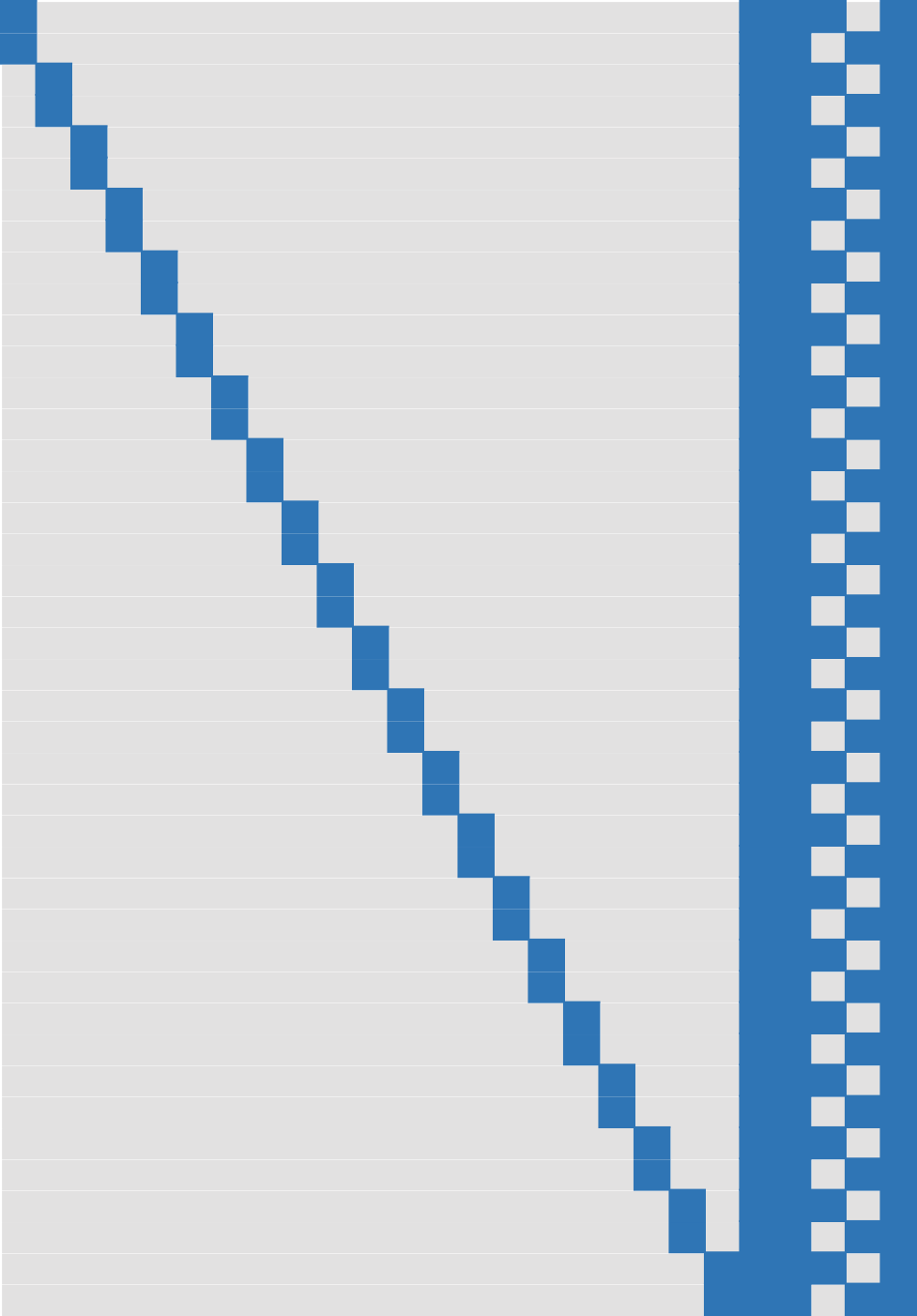
(a) Ellipse fitting

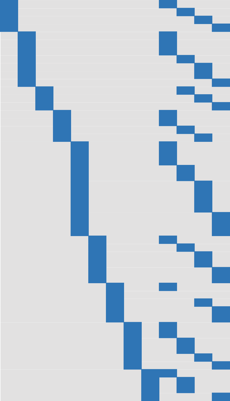
(b) Bundle adjustment

Figure 5: Sparsity patterns of the Jacobian matrix for our benchmark problems.

Figure 6: Performance of different QR factorization methods on the ellipse fitting benchmark.

Problem size	Time [s]
	EigSpQR	SPQR	QRkitBD	QRkitBB
500	0.163	0.016	0.005	0.037
2,000	9.798	0.031	0.017	0.029
10,000	—	0.151	0.098	0.154
100,000	—	1.816	1.036	1.718
500,000	—	9.472	5.342	8.872

Table 1: Timings for different methods on the ellipse fitting benchmark; EigSpQR=Eigen Sparse QR, SPQR=SuiteSparseQR, QRkitBD=QRkit Block Diagonal, QRkitBB=QRkit Block Banded. For Eigen Sparse QR, results are available only up to $N=2000$ as the computation takes too long for bigger problems. The superiority of QRkit is clearly visible.

6.2 Experiments

Surface fitting

is a popular technique for explaining unknown data by fitting a parametric model. In order to show the suitability of QRkit for these problems, we have implemented a simple 2D optimization that fits an ellipse to a set of 2D points. It can be considered a simplification of surface fitting tasks such as human body tracking [33] or hand tracking [37, 38], which have recently received a great deal of interest. The structure of the Jacobian is depicted in Figure 5(a). An efficient solution can be obtained by expressing $J$ as a horizontal concatenation, as described in Section 4.2.

We performed the experiment at different scales. For the number of 2D points $N$, we have performed evaluations for $N$ ranging from $500$ up to $500,000$. Figure 6 shows the comparison of different solvers; the exact timings are then listed in Table 1. We observe that for very small problems ($N\leq 2000$), QRkit performance is comparable to existing methods. As we scale $N$ up to $500,000$, however, QRkit significantly outperforms state-of-the-art implementations, especially when using the block diagonal solver, but also (with a smaller margin) when a block banded solver is used.

Figure 7: Trafalgar (double precision): Convergence comparison of different methods in terms of execution time and number of iterations on the Trafalgar bundle adjustment dataset.

Bundle adjustment

is a simultaneous refinement of 3D coordinates in order to describe geometry of a scene observed by multiple cameras with unknown parameters [1, 40, 41]. The general structure of the Jacobian in a bundle adjustment problem is sketched in Figure 5(b). Its angular structure is efficiently solvable if expressed as a horizontal concatenation (see Section 4.2).

We perform this experiment using standard datasets from GRAIL [1]. In particular, we selected the small version of the and Dubrovnik and Trafalgar Square datasets (the latter we simply call ‘Trafalgar’ below). Each camera is represented by 9 parameters, the 3D points by x,y,z-coordinates and measurements by x,y-coordinates.

Trafalgar consists of 21 cameras capturing 11,315 3D points with a total of 36,455 2D observations. This gives us Jacobian $J\in\mathbb{R}^{n\times m}$ with $n=36455\times 2=72910$ rows and $m=21\times 9+11315\times 3=34134$ columns.

Dubrovnik has only 16 cameras, which capture 22,106 3D points producing 83,718 2D observations. In this case, the Jacobian $J\in\mathbb{R}^{n\times m}$ has $n=83718\times 2=167436$ rows and $m=16\times 9+22106\times 3=66462$ columns.

Figure 8: Trafalgar (single precision): Convergence comparison of different methods in terms of execution time and number of iterations on the Trafalgar bundle adjustment dataset.

Evaluations were performed for both single (32-bit) and double (64-bit) precision floating point. The convergence and execution times in double precision are depicted in Figures 7 and 9. As expected, Cholesky factorization is the fastest here. On the other hand, it does not reach as good an optimum as the Moré QRkit implementation, which suggests better numerical stability of QR for the cost of slower execution. It is worth mentioning that QRkit outperforms the state-of-the-art QR factorization implementation SPQR in terms of execution time and performs on-par with it in terms of convergence (see Table 2).

Results for single precision in terms of convergence and execution times are shown in Figures 8 and 10. It suggests that Cholesky might not be the right choice in this case as it struggles to find a good optimum. On the contrary, QRkit finds an optimum closer to the one achieved in double precision and executes approximately 50% faster. This shows the strong advantage of using QRkit over Cholesky in single precision arithmetic.

Numerical results for both single and double precision are listed in Table 3. In addition, Table 2 displays the minimum energy for each of the methods and both precisions.

Method	Minimum energy
	Trafalgar		Dubrovnik
	Double	Single	Double	Single
Cholesky	1450.34	1517.57	3172.60	3166.51
QRkit	1460.43	1466.59	3171.77	3092.92
QRkit + Chol	1444.10	1494.93	3160.13	3508.25
Moré QRkit	1395.99	1463.50	3128.07	3094.73
SPQR	1436.58	—	3151.63	—
SSBA	1454.19	1531.69	3172.89	3248.25

Table 2: Comparison of the energy minimum found by different methods. The numerical stability of QR is emphasized especially in single precision arithmetic.

Figure 9: Dubrovnik (double precision): Convergence comparison of different methods in terms of execution time and number of iterations on the Dubrovnik bundle adjustment dataset.

Figure 10: Dubrovnik (single precision): Convergence comparison of different methods in terms of execution time and number of iterations on the Dubrovnik bundle adjustment dataset.

Method	Time [s] / Number of iterations
	Trafalgar dataset				Dubrovnik dataset
	Do@1600	Si@1600	Do@1460	Si@1475	Do@3500	Si@3500	Do@3175	Si@3125
Cholesky	2.19 / 5	5.04 / 6	27.05 / 51	—	11.37 / 19	15.93 / 21	73.71 / 112	—
QRkit	12.08 / 5	9.98 / 5	222.25 / 85	138.99 / 51	80.16 / 19	73.22 / 18	551.63 / 116	287.83 / 67
QRkit + Chol	5.98 / 5	5.967 / 6	56.36 / 40	—	58.45 / 19	75.15 / 19	216.05 / 67	—
Moré QRkit	18.14 / 6	12.063 / 6	94.81 / 27	124.70 / 43	123.11 / 21	87.47 / 20	404.27 / 62	298.80 / 55
SPQR	41.28 / 5	—	451.36 / 43	—	282.92 / 19	—	1038.73 / 61	—
SSBA	0.55 / 5	0.38 / 6	6.10 / 41	—	6.99 / 19	4.17 / 21	29.79 / 81	—

Table 3: Timing comparison for different factorization approaches based on both Cholesky and QR, showing the contrast between speed of Cholesky and stability of QR. The header is in the format Precision@Energy, where Do=Double and Si=Single.

7 Conclusions

We presented a new suite of sparsity-aware QR factorizations for the Eigen C++ library. Our QRkit can efficiently deal with matrices that exhibit block diagonal or block banded sparsity patterns and their horizontal or vertical concatenations. QRkit is open source, fully contained in Eigen and does not have any external dependencies. It is therefore a good candidate to become part of the official Eigen release in the near future. We further adapt Eigen’s Levenberg–Marquardt implementation to be able to evaluate our solvers on larger problems.

We performed experiments on a simple surface fitting problem and problems from the standard datasets in bundle adjustment. We show superior performance over the state-of-the-art sparse QR solver SPQR from SuiteSparse. Furthermore, we confirm the better numerical stability of QR over Cholesky decomposition in single precision arithmetic, which holds increasing importance for embedded computer vision applications.

For all tested problems, single precision reached lower energies with QR-based than with Cholesky-based optimizers, regardless of runtime, and for many problems this is a clear advantage of the QR-based methods. These encouraging results motivate us to continue in the proposed direction and revisit the current state-of-the-art in sparse matrix factorization. In order to motivate the community to rethink the abundant use of Cholesky, our future work will show numerous applications of QRkit in latent variable problems.

References

- [1] S. Agarwal, N. Snavely, S. M. Seitz, and R. Szeliski. Bundle adjustment in the large. In Proceedings of the 11th European Conference on Computer Vision: Part II, ECCV’10, pages 29–42, Berlin, Heidelberg, 2010. Springer-Verlag.
- [2] E. Anderson, Z. Bai, J. Dongarra, A. Greenbaum, A. McKenney, J. Du Croz, S. Hammarling, J. Demmel, C. Bischof, and D. Sorensen. LAPACK: A portable linear algebra library for high-performance computers. In Proceedings of the 1990 ACM/IEEE Conference on Supercomputing, Supercomputing ’90, pages 2–11, Los Alamitos, CA, USA, 1990. IEEE Computer Society Press.
- [3] M. Baboulin, A. Buttari, J. Dongarra, J. Kurzak, J. Langou, J. Langou, P. Luszczek, and S. Tomov. Accelerating scientific computations with mixed precision algorithms. Computer Physics Communications, 180(12):2526 – 2533, 2009.
- [4] C. Bischof and C. V. Loan. The WY representation for products of householder matrices. SIAM Journal on Scientific and Statistical Computing, 8(1):s2–s13, 1987.
- [5] Å. Björck. Numerics of Gram-Schmidt orthogonalization. Linear Algebra and its Applications, 197-198(Supplement C):297 – 316, 1994.
- [6] Å. Björck. Numerical Methods in Matrix Computations. Texts in Applied Mathematics. Springer International Publishing, 2014.
- [7] A. Buttari, J. Langou, J. Kurzak, and J. Dongarra. Parallel tiled QR factorization for multicore architectures. Concurrency and Computation: Practice and Experience, 20(13):1573–1590, 2008.
- [8] C. Cadena, L. Carlone, H. Carrillo, Y. Latif, D. Scaramuzza, J. Neira, I. Reid, and J. J. Leonard. Past, present, and future of simultaneous localization and mapping: Toward the robust-perception age. IEEE Transactions on Robotics, 32(6):1309–1332, 2016.
- [9] T. J. Cashman and A. W. Fitzgibbon. What shape are dolphins? Building 3D morphable models from 2D images. IEEE Transactions on Pattern Analysis and Machine Intelligence, 35(1):232–244, 2013.
- [10] A. R. Conn, N. I. M. Gould, and P. L. Toint. Trust-region Methods. Society for Industrial and Applied Mathematics, Philadelphia, PA, USA, 2000.
- [11] M. Cosnard, J. M. Muller, and Y. Robert. Parallel QR decomposition of a rectangular matrix. Numerische Mathematik, 48(2):239–249, 1986.
- [12] T. A. Davis. Algorithm 915, SuiteSparseQR: Multifrontal multithreaded rank-revealing sparse QR factorization. ACM Trans. Math. Softw., 38(1):8:1–8:22, 2011.
- [13] T. A. Davis, J. R. Gilbert, S. I. Larimore, and E. G. Ng. A column approximate minimum degree ordering algorithm. ACM Trans. Math. Softw., 30(3):353–376, 2004.
- [14] J. Demmel, L. Grigori, M. Hoemmen, and J. Langou. Communication-avoiding parallel and sequential QR factorizations. CoRR, abs/0806.2159, 2008.
- [15] J. G. F. Francis. The QR transformation a unitary analogue to the LR transformation - part 1. The Computer Journal, 4(3):265–271, 1961.
- [16] J. G. F. Francis. The QR transformation - part 2. The Computer Journal, 4(4):332–345, 1962.
- [17] W. Gander. Algorithms for the QR decomposition. Seminar für Angewandte Mathematik: Research report. 1980.
- [18] W. Givens. Computation of plane unitary rotations transforming a general matrix to triangular form. Journal of the Society for Industrial and Applied Mathematics, 6(1):26–50, 1958.
- [19] G. H. Golub and C. Reinsch. Singular value decomposition and least squares solutions. Numerische Mathematik, 14(5):403–420, 1970.
- [20] G. Guennebaud, B. Jacob, et al. Eigen v3. http://eigen.tuxfamily.org, 2010.
- [21] B. C. Gunter and R. A. Van De Geijn. Parallel out-of-core computation and updating of the QR factorization. ACM Trans. Math. Softw., 31:60–78, 2005.
- [22] M. D. Hebden. An algorithm for minimization using exact second derivatives. Technical report, Atomic Energy Research Establishment report TP515, Harwell, England, 1973.
- [23] A. S. Householder. A class of methods for inverting matrices. Journal of the Society for Industrial and Applied Mathematics, 6(2):189–195, 1958.
- [24] V. Kublanovskaya. On some algorithms for the solution of the complete eigenvalue problem. USSR Computational Mathematics and Mathematical Physics, 1(3):637 – 657, 1962.
- [25] J. Langou, P. Luszczek, J. Kurzak, A. Buttari, and J. Dongarra. Exploiting the performance of 32 bit floating point arithmetic in obtaining 64 bit accuracy (revisiting iterative refinement for linear systems). In SC 2006 Conference, Proceedings of the ACM/IEEE, pages 50–50, 2006.
- [26] C. L. Lawson, R. J. Hanson, D. R. Kincaid, and F. T. Krogh. Basic linear algebra subprograms for Fortran usage. ACM Trans. Math. Softw., 5(3):308–323, 1979.
- [27] K. Levenberg. A method for the solution of certain non-linear problems in least squares. Quarterly of Applied Mathematics, 2(2):164–168, 1944.
- [28] M. I. A. Lourakis and A. A. Argyros. SBA: A software package for generic sparse bundle adjustment. ACM Trans. Math. Softw., 36(1):2:1–2:30, 2009.
- [29] D. W. Marquardt. An algorithm for least-squares estimation of nonlinear parameters. Journal of the Society for Industrial and Applied Mathematics, 11(2):431–441, 1963.
- [30] J. J. Moré. Levenberg–Marquardt algorithm: implementation and theory. 1977.
- [31] J. J. Moré and D. C. Sorensen. Computing a trust region step. SIAM J. Sci. Stat. Comput., 4(3):553–572, 1983.
- [32] D. P. O’Leary and P. Whitman. Parallel QR factorization by Householder and modified Gram-Schmidt algorithms. Parallel Computing, 16(1):99 – 112, 1990.
- [33] X. Perez-Sala, S. Escalera, and J. González. A survey on model based approaches for 2D and 3D visual human pose recovery. Sensors, 14(3):189–210, 2014.
- [34] A. Roldao-Lopes, A. Shahzad, G. A. Constantinides, and E. C. Kerrigan. More flops or more precision? accuracy parameterizable linear equation solvers for model predictive control. In 2009 17th IEEE Symposium on Field Programmable Custom Computing Machines, pages 209–216, 2009.
- [35] R. Schreiber and B. Parlett. Block reflectors: Theory and computation. SIAM Journal on Numerical Analysis, 25(1):189–205, 1988.
- [36] R. Schreiber and C. van Loan. A storage-efficient WY representation for products of householder transformations. SIAM J. Sci. Stat. Comput., 10(1):53–57, 1989.
- [37] A. Tagliasacchi, M. Schroeder, A. Tkach, S. Bouaziz, M. Botsch, and M. Pauly. Robust Articulated-ICP for real-time hand tracking. Computer Graphics Forum (Proc. Symposium on Geometry Processing), 2015.
- [38] J. Taylor, L. Bordeaux, T. Cashman, B. Corish, C. Keskin, T. Sharp, E. Soto, D. Sweeney, J. Valentin, B. Luff, A. Topalian, E. Wood, S. Khamis, P. Kohli, S. Izadi, R. Banks, A. Fitzgibbon, and J. Shotton. Efficient and precise interactive hand tracking through joint, continuous optimization of pose and correspondences. ACM Trans. Graph., 35(4):143:1–143:12, 2016.
- [39] C. Tomasi and T. Kanade. Shape and motion from image streams under orthography: a factorization method. International Journal of Computer Vision, 9(2):137–154, 1992.
- [40] B. Triggs, P. F. McLauchlan, R. I. Hartley, and A. W. Fitzgibbon. Bundle Adjustment — A Modern Synthesis, pages 298–372. Springer Berlin Heidelberg, Berlin, Heidelberg, 2000.
- [41] C. Zach. Robust bundle adjustment revisited. In Computer Vision–ECCV 2014, pages 772–787. Springer, 2014.