Dark matter: An efficient catalyst for intermediate-mass-ratio-inspiral events

Abstract

Gravitational waves (GWs) can be produced if a stellar compact object, such as a black hole (BH) or neutron star, inspirals into an intermediate-massive black hole (IMBH) of $(10^{3}\sim 10^{5})\,M_{\odot}$. Such a system may be produced in the center of a globular cluster (GC) or a nuclear star cluster (NSC), and is known as an intermediate- or extreme-mass-ratio inspiral (IMRI or EMRI). Motivated by the recent suggestions that dark matter minispikes could form around IMBHs, we study the effect of dynamical friction against DM on the merger rate of IMRIs/EMRIs. We find that the merger timescale of IMBHs with BHs and NSs would be shortened by two to three orders of magnitude. As a result, the event rate of IMRIs/EMRIs are enhanced by orders of magnitude relative to that in the case of no DM minispikes. In the most extreme case where IMBHs are small and the DM minispikes have a steep density profile, all the BH in GCs and NSCs might be exhausted so that the mergers with NSs would dominate the current IMRIs/EMRIs. Our results suggest that the mass function of the IMBHs below $10^{4}\,M_{\odot}$ would bear imprints of the distribution of DM minispikes because these low-mass IMBHs can grow efficiently in the presence of DM minispikes by merging with BHs and NSs. Future space-based GW detectors, like LISA, Taiji, and Tianqin, can measure the IMRI/EMRI rate and hence constrain the distribution of DM around IMBHs.

1 Introduction

Cosmological and astrophysical observations have provided reliable evidence for the existence of dark matter (DM). It is important to understand the distribution of DM in different astrophysical systems. Navarro et al. (1997) first pointed out a universal density profile for DM halos called the NFW profile. Gondolo & Silk (1999) suggested that the adiabatic growth of a supermassive black hole (SMBHs) with a mass $M\sim 10^{6-9}M_{\odot}$ at the center of a galaxy can create a high density cusp of DM called the DM "spike." However, the DM spikes could be removed by astrophysical processes such as galaxy mergers, formation of off-centered seed BHs, and scattering with the surrounding stars (Merritt et al., 2002; Ullio et al., 2001; Merritt, 2004; Bertone et al., 2005).

On the other hand, DM minispikes may exist around an intermediate-massive black hole (IMBH) with a mass of $M\sim 10^{3-5}M_{\odot}$. In particular, it has been shown that spinning IMBHs could have formed minispikes more easily (Ferrer et al., 2017). Although the formation process of IMBHs is still unclear, there is an increasing number of evidence suggesting that they should exist in the centers of globular clusters (GCs) or the nuclear stellar clusters (NSCs) of dwarf galaxies. The active galactic galactic nuclei (AGNs) in dwarf galaxies provide robust evidence supporting the existence of $\approx 10^{5}M_{\odot}$ BHs. Another strong piece of evidence is the ultra-luminous X-ray sources (Farelletal.09; 2010;Feng&Soria2011). The final proof of the existence of IMBHs requires detection of the innermost stellar kinematics in GCs or NSCs, which is still difficult to achieve today. Nevertheless, if minispikes exist around IMBHs, they are less likely to be destroyed by galaxy mergers because their hosts may not have experienced major mergers in the past (Zhao & Silk, 2005; Bertone et al., 2005).

The recent detection of gravitational waves (GWs) opened a new possibility of proving the existence of IMBHs. If a stellar-mass black hole (BH) orbits around an IMBH or SMBH, the two objects form an intermediate-mass-ratio inspiral (IMRI, of a mass ratio of $10^{-2}\sim 10^{-3}$) or an extreme-mass-ratio inspiral (EMRI, with a mass ratio of $10^{-4}\sim 10^{-6}$). Such a system is an ideal source for the space-borne detectors such as LISA (Amaro-Seoane et al., 2013, 2017), Tianqin (Gong et al., 2011), and Taiji (Luo et al., 2016). It was estimated in Miller & Hamilton (2002) that there are 10 IMRIs in the LISA band at any time. Moreover, if the mass of the IMBH is $\lesssim 10^{3}M_{\odot}$, the final merger phase of the IMBH and the stellar BH could be detected by the advanced LIGO (Mandel et al., 2008; Amaro-Seoane et al., 2009).

Detecting IMBHs via GWs would also allow us to test the existence of DM minispikes. For example, Eda et al. (2013) showed that the additional gravitational attraction due to the DM minispike can affect the waveform of an EMRI, and the deviate of the observed waveform from a standard EMRI template is detectable by LISA. Furthermore, Eda et al. (2015) showed that the dynamical friction of the DM could also induce an observable effect on the EMRI waveform. In addition, Yue & Han (2018) considered the combined effect of gravitational pulling, dynamical friction, and the accretion of DM, and showed that the dynamical friction is predominant.

Based on the results of the previous studies, here we calculate the merger times for the IMRIs/EMRIs embedded in DM minispikes (Sec.2). We use them to further derive the event rates in GCs (Sec.3) and the NSCs in dwarf galaxies (Sec.4). We discuss the robustness of our results in Section 5 and provide our conclusions in Section 6.

2 Merger time in DM minispikes

Our DM minispike is the same as that derived in Eda et al. (2015), whose density $\rho$ follows a power-law distribution of

$$\rho(r)=\rho_{\rm sp}\left(\frac{r_{\rm sp}}{r}\right)^{\alpha},$$ (1)

where $r_{\rm sp}$ is a typical scale radius normally related to the influence radius $r_{h}$ of the central massive black hole (MBH) as $r_{\rm sp}\sim 0.2r_{h}$ and $\rho_{\rm sp}$ is the DM density at $r=r_{\rm sp}$. The influence radius can be calculated from the equation $4\pi\int_{0}^{r_{h}}\rho_{\rm DM}r^{2}dr=2M_{\rm BH}$ where $M_{\rm BH}$ denotes the mass of the central MBH. Following the derivation in Eda et al. (2015), we use $r_{\rm sp}\simeq 0.54\,{\rm pc}$ and $\rho_{\rm sp}=226\,M_{\odot}/{\rm pc}^{3}$ throughout this paper. We note that in principle $\rho_{\rm sp}$ and $r_{\rm sp}$ should depend on the mass of the central MBH, but the relationship has not been derived in the literature . Therefore, for simplicity, here we use the same values of $\rho_{\rm sp}$ and $r_{\rm sp}$ for the IMBHs in the mass range of $10^{3-5}M_{\odot}$.

As for the power-law index $\alpha$, it can be derived according to the model of adiabatic growth of massive black holes (MBHs, see Young., 1980). If the initial DM halo, prior to the formation of the MBH, has a NFW profile with an initial power-law index of $\alpha_{\rm ini}=1$ (Navarro et al., 1997), the index after the adiabatic growth of the MBH is $\alpha=(9-2\alpha_{\rm ini})/(4-\alpha_{\rm ini})=7/3$ (Ullio et al., 2001; Quinian et al., 1995). Alternatively, if the initial halo has a uniform density distribution, the final power-law index is $\alpha=1.5$ (Ullio et al., 2001; Quinian et al., 1995). For these reasons, we will assume $1.5<\alpha<7/3$ in the following analysis.

We now consider a binary composed of an IMBH with a mass of $M_{\rm BH}\sim 10^{3-5}M_{\odot}$ and a compact object such as a stellar-mass BH with a mass of $\mu=10M_{\odot}$ or a neutron star (NS) with $\mu=1.4M_{\odot}$. The binary is embedded in the center of the DM minispike. Since the mass of the secondary compact object is much smaller than the central IMBH, the reduced mass of the binary is approximately $\mu$ and the center-of-mass is approximately at the position of the IMBH.

In the Newtonian formalism, the motion of the secondary compact object can be decomposed into a radial component and a tangential one. The equation of motion in the radial direction is $\mu\ddot{r}-\mu r\dot{\theta}^{2}=F$, where $F$ is the gravitational force imposed by the IMBH as well as the DM minispike. Inside the radius of the innermost stable orbit, i.e., $r<r_{\rm ISCO}$, there is no stable orbit for DM particles so that they all fall into the central hole. As a result, the DM has a hollow distribution around the IMBH and this needs to be accounted for in the calculation of the gravitational force. In the end the equation in the radial direction can be written in the form (Eda et al., 2013)

$$\mu\ddot{r}-\mu r\dot{\theta}^{2}=-\frac{G\mu M_{\rm eff}}{r^{2}}-\frac{\mu F}{r^{\alpha-1}},$$ (2)

where

$$M_{\rm eff} =\begin{cases}M_{\rm BH}-M_{\rm DM}(<r_{\rm min}),&\text{$r_{\rm min}<r<r_{\rm sp}$},\\ M_{\rm BH},&\text{$r<r_{\rm min}$},\\ \end{cases}$$ (3)

$$F =\begin{cases}Gr_{\rm min}^{\alpha-3}M_{\rm DM}(<r_{\rm min}),&\text{$r_{\rm min}<r<r_{\rm sp}$},\\ 0,&\text{$r<r_{\rm min}$}.\end{cases}$$ (4)

In the above equations, $r_{\rm min}=r_{\rm ISCO}=6GM_{\rm BH}/c^{2}$ is the radius of the innermost stable circular orbit (ISCO) and $M_{\rm DM}(<r_{\rm min})=4\pi r_{\rm sp}^{\alpha}\rho_{\rm sp}r_{\rm min}^{\alpha-3}/(3-\alpha)$ is the DM contained in $r_{\rm ISCO}$. The first term on the right-hand side of Equation (2) is the effective mass of IMBH corrected by DM. The second is the gravitational effect of DM. For a circular orbit, $\ddot{r}=0$, and

$$\dot{\theta}=\omega_{s}=\sqrt{\frac{GM_{\rm eff}}{r^{3}}+\frac{F}{r^{\alpha}}}$$ (5)

is the orbital frequency.

As the secondary compact object moves in the DM minispike, its orbital energy is lost due to GW radiation and the dynamical friction against the DM background. The equation of energy balance is

$$-\frac{dE_{\rm orbit}}{dt}=\frac{dE_{\rm GW}}{dt}+\frac{dE_{\rm DF}}{dt},$$ (6)

where the terms are explained in as follows. The orbit energy is

$$E_{\rm orbit} =\frac{1}{2}\mu v^{2}-\frac{G\mu M_{\rm eff}}{r}+\frac{1}{2-\alpha}\frac{\mu F}{r^{\alpha-2}}$$ (7)

$$=-\frac{G\mu M_{\rm eff}}{2r}+\frac{4-\alpha}{2(2-\alpha)}\frac{\mu F}{r^{\alpha-2}},$$

where $v$ is the circular velocity of the small body. The rate of energy loss via GWs is

$$\frac{dE_{\rm DF}}{dt}=\frac{32}{5}\frac{G\mu^{2}}{c^{5}}r^{4}\omega_{s}^{6}.$$ (8)

The force due to dynamical friction is $f_{\rm DF}=4\pi G^{2}\mu^{2}\rho_{\rm DM}(r)\ln\Lambda/v^{2}$ and the corresponding energy dissipation rate is

$$\frac{dE_{\rm DF}}{dt}=vf_{\rm DF}=4\pi G^{2}\frac{\mu^{2}\rho_{\rm DM}(r)}{v}\ln\Lambda\,.$$ (9)

where $\ln\Lambda$ is the Coulumb logarithm and we assume $\ln\Lambda=10$. Replacing the terms in Equation (6) using Equations (1), (7), (8), and (9), we find

$$\frac{dr}{dt}= -\left(\frac{GM_{\rm eff}}{2r^{2}}+\frac{4-\alpha}{2}\frac{F}{r^{\alpha-1}}\right)^{-1}$$ (10)

$$\times\left[\frac{32}{5}\frac{G\mu}{c^{5}}r^{4}\omega_{s}^{6}+\frac{4\pi G^{2}\mu\rho_{\rm sp}r_{\rm sp}^{\alpha}\ln\Lambda}{r^{\alpha+1}\omega_{s}}\right],$$

where $\omega_{s}$ is derived in Equation (5). For example, if the DM minispike is absent, $F=0$ and the second term in the brackets vanishes, and hence Equation (10) reduces to

$$\frac{dr}{dt}=-\frac{64}{5}\frac{G^{3}\mu M^{2}}{c^{5}r^{3}},$$ (11)

which is the well-known Peters formula (Peters & Mathews, 1963).

Using Equations (10) or(11), we can derive the merger time from an initial radius of $r$ to the final radius $r_{\rm ISCO}$, which is

$$T_{\rm merge}=\int_{r}^{r_{\rm ISCO}}\frac{dt}{dr}dr.$$ (12)

Figures 1-3 illustrate our results of the merger times for different parameters $\alpha$ and different masses of IMBH. It is clear that the presence of DM minispikes greatly reduces the merger times of IMRIs. We note that $T_{\rm merge}$ is approximately the evolution timescale at $r$ due to GW radiation and DM friction, because the time spent at $r$ is much longer than that at $r_{\rm ISCO}$.

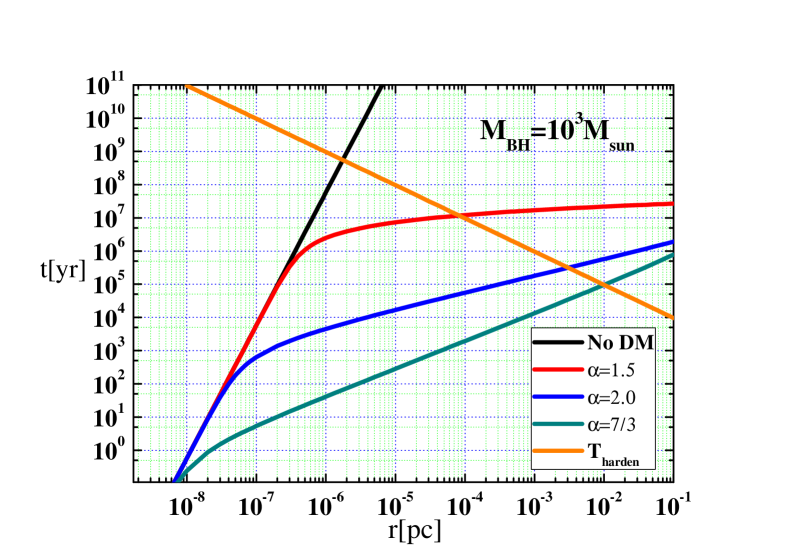
Figure 1: Merger time for an IMRI with $\mu=10\,M_{\odot}$ and $M_{\rm BH}=10^{3}M_{\odot}$ computed using different DM density profiles (the black, red, blue, and green curves), as well as the hardening time due to scattering away DM particles (orange line).

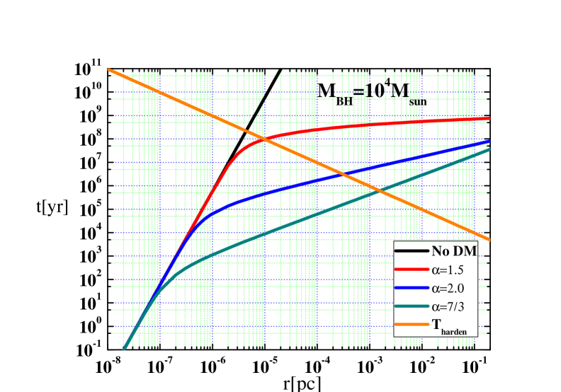
Figure 2: Same as Figure 1 but for $M_{\rm BH}=10^{4}\,M_{\odot}$.

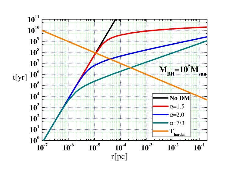
Figure 3: Same as Figure 1 but for $M_{\rm BH}=10^{5}\,M_{\odot}$.

Besides the dynamical friction against the DM background, another competing mechanism that could also extract the orbital energy from the binary of IMBH and stellar BH is “dynamical hardening” (Heggie, 1975; Gürkan et al., 2006; Mandel et al., 2008). According to this mechanism, a stellar interloper could interact with the binary in a complicated way such that by the end of the interaction the interloper is reejected into the background, taking away a fraction of the energy and angular momentum from the binary.

To study the relative efficiency of the dynamical hardening, we adopt the method of Quinlan (1996) and calculate the hardening rate using

$$\frac{da}{dt}=-\frac{GH\rho a^{2}}{\sigma},$$ (13)

where $a$ is the semi-major axis of the binary, $H\sim 15$ is a constant, $\rho$ is the typical density of the background stars, and $\sigma$ is the velocity dispersion of these stars. For simplicity, we assume that $\rho$ is constant, which mimics the core profile observed in the centers of many massive GCs. Moreover, we do not consider a significant eccentricity $e$ for our binaries, i.e., we have $a=r$. Finally, the hardening timescale from the initial radius $r_{i}$ to the final one $r$ is

$$T_{\textrm{harden}}=\int^{r}_{r_{i}}\left(\frac{dt}{dr}\right)_{\textrm{harden}}dr,$$ (14)

where $(dt/dr)_{\textrm{harden}}$ is from Equation (13). We note that the choice of $r_{i}$ is not important for the calculation of $T_{\textrm{harden}}$ because $(dt/dr)_{\textrm{harden}}$ quickly approaches $0$ as $r$ increases. For this reason, we assume $r_{i}=\infty$ in our calculations and the value given by Equation (13) is approximately the hardening timescale at the radius $r$, since the IMRIs/EMRIs evolve much slower at smaller $r$. By solving for the radius where $T_{\textrm{harden}}=T_{\rm merge}$, we can find the transition radius of the two processes. These critical radii are shown in Figures 1-3 as the intersections of the lines of $T_{\rm merge}$ and $T_{\rm harden}$.

For example, if we use the typical parameters for GCs, i.e., $\sigma=10\,{\rm km\,s^{-1}}$, $\rho=nm_{\ast}$ where $n=10^{5.5}\,{\rm pc}^{-3}$ is the number density of stars, and $m_{\ast}=0.5\,M_{\odot}$ is the average mass for a single star (Pryor & Meylan, 1993), we can compute the corresponding $T_{\textrm{harden}}$ ,which are shown in Figures (1)-(3) as the oranges lines. Comparing these results with $T_{\rm merge}$, we find that in general the effect of dynamical hardening is more important at large radius and subsides as the semi-major axis of the binary shrinks.

Since both the DM and dynamical hardening are affecting the evolution, the total shrinking rate due to the two effects combined is

$$\left(\frac{dr}{dt}\right)_{\textrm{total}}=\left(\frac{dr}{dt}\right)_{1}+\left(\frac{dr}{dt}\right)_{2},$$ (15)

where $(dr/dt)_{1}$ is the rate due to GW and DM, which is computed from Equation (10), and $(dr/dt)_{2}$ is the hardening rate from Equation (13). Correspondingly, the total merger time combining the two effects is

$$T=\int_{r_{i}}^{r_{\textrm{ISCO}}}\left(\frac{dt}{dr}\right)_{\textrm{total}}dr=\int_{r_{i}}^{r_{\textrm{ISCO}}}\frac{1}{\left({dr}/{dt}\right)_{1}+\left({dr}/{dt}\right)_{2}}.$$ (16)

Numerically, the value of $T$ is determined mainly at the radius where $T_{\rm merge}\simeq T_{\rm harden}$.

3 Merger rate in GCs

3.1 Merger rate in a single GC

To calculate the merger rate of IMRIs in an GC, besides the merger time $T$ calculated in the previous section, we also need to know the supply rate of compact stellar objects, such as BHs and NSs, to the center where the IMBH presumably resides. On one hand, if this rate is lower than the reciprocal of the merger time ($1/T$), the formation of IMRIs would be limited by the supply rate, and the merger rate, consequently, is equal to it as well. On the other, if the supply rate is higher than $1/T$, we expect two stellar compact objects to arrive at the cluster center around the same time to form a triple system with the IMBH. However, such a triple is almost always unstable and will likely eject the lightest component. The result would be a tighter IMRI, which continues to eject future stellar interlopers via dynamical hardening (see previous section) until the IMRI coalesces. In this case, the average duration between two successive mergers is limited by the merger time $T$, and, consequently, the merger rate is $1/T$.

Following Gair et al. (2017), we relate the supply rate of BHs and NSs to the regrow timescale, $t_{\rm cusp}$, of the stellar cusp around an IMBH. This timescale depends on the size of the core scoured out by the hardening process of the former IMRI and can be calculated approximately by

$$t_{\rm cusp}\approx 6\left(\frac{M}{10^{6}M_{\odot}}\right)^{1.19}q^{0.35}\rm Gyr,$$ (17)

where $M$ is the total mass of the IMRI and $q$ is the mass ratio between the IMBH and the companion compact object (Babak et al., 2017). Correspondingly, supply rate is $1/(2t_{\rm cusp})$, where the factor of $2$ accounts for uncertainties such as the time delay between cusp regeneration and IMRI formation.

Table 1 summarizes our results for the calculation of the merger rate. It is clear that with DM minispikes, the merger rate is significantly enhanced. Figure (4) shows the merger rate of an IMBH with stellar BHs as a function of the mass of the IMBH. We find that the presence of a DM minispikes changes the relation between the merger rate and the IMBH mass.

Table 1: The reciprocal of the merger time, the supply rate of BHs to the vicinity of IMBHs to form IMRIs, the merger rate, and the duty cycle of IMRIs/EMRIs for different dark matter density profiles in a GC.

$M=10^{3}M_{\odot}$	1/T	Supply Rate	Merger Rate	Duty Cycle
No DM	$1.3\times 10^{-9}\textrm{yr}^{-1}$	$1.5\times 10^{-6}\textrm{yr}^{-1}$	$1.3\times 10^{-9}\textrm{yr}^{-1}$	$T_{\textrm{Hubble}}$
$\alpha=1.5$	$6.5\times 10^{-8}\textrm{yr}^{-1}$	$1.5\times 10^{-6}\textrm{yr}^{-1}$	$6.5\times 10^{-8}\textrm{yr}^{-1}$	$T_{\textrm{Hubble}}$
$\alpha=2.0$	$2.1\times 10^{-6}\textrm{yr}^{-1}$	$1.5\times 10^{-6}\textrm{yr}^{-1}$	$1.5\times 10^{-6}\textrm{yr}^{-1}$	$6.7\times 10^{8}\textrm{yr}$
$\alpha=7/3$	$6.6\times 10^{-6}\textrm{yr}^{-1}$	$1.5\times 10^{-6}\textrm{yr}^{-1}$	$1.5\times 10^{-6}\textrm{yr}^{-1}$	$6.7\times 10^{8}\textrm{yr}$

$M=10^{4}M_{\odot}$	1/T	Supply Rate	Merger Rate	Duty Cycle
No DM	$3.3\times 10^{-9}\textrm{yr}^{-1}$	$2.2\times 10^{-7}\textrm{yr}^{-1}$	$3.3\times 10^{-9}\textrm{yr}^{-1}$	$T_{\textrm{Hubble}}$
$\alpha=1.5$	$7.4\times 10^{-9}\textrm{yr}^{-1}$	$2.2\times 10^{-7}\textrm{yr}^{-1}$	$7.4\times 10^{-9}\textrm{yr}^{-1}$	$T_{\textrm{Hubble}}$
$\alpha=2.0$	$2.1\times 10^{-7}\textrm{yr}^{-1}$	$2.2\times 10^{-7}\textrm{yr}^{-1}$	$2.1\times 10^{-7}\textrm{yr}^{-1}$	$4.8\times 10^{9}\textrm{yr}$
$\alpha=7/3$	$1.0\times 10^{-6}\textrm{yr}^{-1}$	$2.2\times 10^{-7}\textrm{yr}^{-1}$	$2.2\times 10^{-7}\textrm{yr}^{-1}$	$4.5\times 10^{9}\textrm{yr}$

$M=10^{5}M_{\odot}$	1/T	Supply Rate	Merger Rate	Duty Cycle
No DM	$8.2\times 10^{-9}\textrm{yr}^{-1}$	$3.2\times 10^{-8}\textrm{yr}^{-1}$	$8.2\times 10^{-9}\textrm{yr}^{-1}$	$T_{\textrm{Hubble}}$
$\alpha=1.5$	$8.3\times 10^{-9}\textrm{yr}^{-1}$	$3.2\times 10^{-8}\textrm{yr}^{-1}$	$8.3\times 10^{-9}\textrm{yr}^{-1}$	$T_{\textrm{Hubble}}$
$\alpha=2.0$	$2.7\times 10^{-8}\textrm{yr}^{-1}$	$3.2\times 10^{-8}\textrm{yr}^{-1}$	$2.7\times 10^{-8}\textrm{yr}^{-1}$	$T_{\textrm{Hubble}}$
$\alpha=7/3$	$1.6\times 10^{-7}\textrm{yr}^{-1}$	$3.2\times 10^{-8}\textrm{yr}^{-1}$	$3.2\times 10^{-8}\textrm{yr}^{-1}$	$T_{\textrm{Hubble}}$

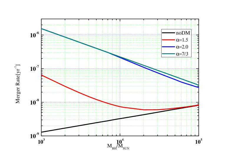
Figure 4: Merger rate of BHs in a GC with different DM density profiles as a function of the mass of the central IMBH.

Since the presence of DM minispikes can enhance the merger rate of IMBHs with stellar BHs, a GC could be quickly deprived of stellar BHs and no longer produce any IMRIs. To quantify this probability, we calculate the duty cycles for the production of IMRIs by our GCs, and the results are given in the last column of Table 1. In our calculations we assume that each GC on average has $1000$ stellar BHs. This number is derived based on the facts that (1) a typical GC has $10^{6}$ stars, (2) about $0.3\%$ of them will turn into BHs if the initial mass function (IMF) for stars is Salpeter and the progenitor stars of BHs are more massive than $30M_{\odot}$, and (3) a large fraction of the newborn BHs will receive natal kicks that are greater than the escape velocity of the GC. As a result, the GCs with a merger rate greater than about $10^{-7}{\rm yr^{-1}}$ would deplete their stellar BHs within a Hubble time. The relevant GCs, according to Figure (4), are those less massive than $2\times 10^{4}M_{\odot}$ and with a DM density profile of $\alpha\geq 2.0$.

Besides depleting the stellar BHs in a cluster, another effect of the high merger rate of IMRIs is to increase the mass of the IMBH on a timescale much shorter than the Hubble time (see Table 1). For example, when $M_{\rm BH}=1000\,M_{\odot}$, the IMBH could grow to $2000M_{\odot}$ in less than $10^{8}{\rm yrs}$ if $\alpha=7/3$, and after $5\,{\rm Gyrs}$ even to $\sim 10^{4}M_{\odot}$. Such a rapid increment in mass would have a strong impact on the structure of the star cluster around the IMBH and hence affect our calculations of the merger rate and duty cycle, but our current model is not capable of capturing this effect yet. Alternatively, if $\alpha<1.5$ or the mass is $M_{\rm BH}>2\times 10^{4}\,M_{\odot}$, the growth time would exceed the Hubble time and we can neglect the accretion of BHs by IMBH in our model. The implication of these results is that we could use IMRIs to constrain the mass function of IMBHs and hence further test the DM models in GCs

After the exhaustion of BHs, the formation of IMRIs/EMRIs with NSs becomes important. Table (2) and Figure (5) show the merger rates for NSs, which are calculated in a way similar to the BH merger rates but using $\mu=1.4\,M_{\odot}$. The maximum mass that we consider here for IMBH-NS mergers is $M_{\rm BH}=1\sim 3\times 10^{4}M_{\odot}$, because more massive IMBHs could not deplete all the BHs in the host clusters. The results for IMBH-NS mergers should be taken with caution because we calculated the hardening rate using Equation (13), which is derived under the assumption that the intruding stars are less massive than the smaller member of the IMRI/EMRI. This assumption may be invalid when the IMRI/EMRI involves an NS. With a Salpeter mass function and the assumption that stars within $10M_{\odot}$ and $30M_{\odot}$ will form NSs, we find that NSs in GCs will not be exhausted in our models.

Table 2: The merger rate of IMRIs or EMRIs with neutron stars for different dark matter density profiles in a GC.

	$M=10^{4}M_{\odot}$	$M=2\times 10^{4}M_{\odot}$	$M=3\times 10^{4}M_{\odot}$
$\alpha=2.0$	$5.9\times 10^{-8}\rm yr^{-1}$	$3.1\times 10^{-8}\rm yr^{-1}$	$2.2\times 10^{-8}\rm yr^{-1}$
$\alpha=7/3$	$3.6\times 10^{-7}\rm yr^{-1}$	$2.0\times 10^{-7}\rm yr^{-1}$	$1.5\times 10^{-7}\rm yr^{-1}$

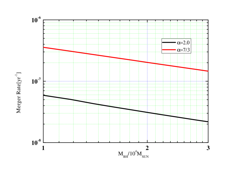
Figure 5: Same as Figure 4 but for IMBH-NS mergers in GCs.

Having derived the merger rate for BHs and NSs, we can study the growth of IMBH during one Hubble time. The results are shown in Figure 6 as a function of the initial masses of the IMBHs. We find that in the presence of DM minispikes, the growth of IMBHs cannot be neglected when the intial masses are small. Alternatively, when there is no minispike, the growth of IMBHs due to the mergers with BHs can be neglected.

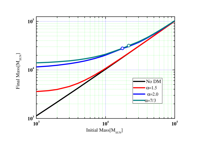
Figure 6: Final masses of IMBHs after 10 Gyr for different initial masses of IMBHs and density profiles of DM cusps in GCs. The circles mark the critical masses below which the IMBHs cannot deplete all the stellar BHs in the clusters. The corresponding initial masses are about $17,600M_{\odot}$ for $\alpha=2.0$ and $21,700M_{\odot}$ for $\alpha=7/3$.

3.2 Merger rate in GCs per $\rm Mpc^{3}$

To derive the merger rate of IMRIs/EMRIs per unit volume, we first calculate the number of GCs in a single galaxy. We adopt the conventional assumption that a fraction of $f_{\rm gc}=0.05$ of stars are in clusters (Kruijssen, 2012; Gnedin et al., 2014), and the mass function of GCs follows a power law $dn/dm_{\rm gc}\propto m_{\rm gc}^{-2}$, where $m_{\rm gc}$ is the cluster mass whose limits are $m_{\rm min}=10^{2}M_{\odot}$ and $m_{\rm max}=10^{7}M_{\odot}$ (Bik et al., 2003; de Grijs et al., 2003). Then given the mass of a galaxy, $\mathcal{M}$, the GC mass function is

$$\frac{dn}{dm_{\rm gc}}=\frac{0.05\mathcal{M}}{\ln(10^{5})m_{\rm gc}^{2}}.$$ (18)

Second, we calculate the number of galaxies per unit volume. According to Baldry et al. (2008), the field galaxy stellar-mass function is

$$\phi_{\mathcal{M}}d\mathcal{M}=e^{-\mathcal{M}/\mathcal{M}_{\ast}}\left[\phi_{1}^{\ast}\left(\frac{\mathcal{M}}{\mathcal{M}_{\ast}}\right)^{\alpha_{1}}+\phi_{2}^{\ast}\left(\frac{\mathcal{M}}{\mathcal{M}_{\ast}}\right)^{\alpha_{2}}\right]\frac{d\mathcal{M}}{\mathcal{M}_{\ast}},$$ (19)

where $\phi_{\mathcal{M}}d\mathcal{M}$ is the number density of galaxies within the mass bin between $\mathcal{M}$ and $\mathcal{M}+d\mathcal{M}$. The best- fitting parameters are

$$\log(\mathcal{M}/M_{\odot}) =10.648$$

$$\phi_{1}^{\ast}/(10^{-3}\rm Mpc^{-3}) =4.26,\alpha_{1}=-0.46$$

$$\phi_{2}^{\ast}/(10^{-3}\rm Mpc^{-3}) =0.58,\alpha_{2}=-1.58.$$ (20)

Third, we derive the number density of GCs as

$$n=\int_{\mathcal{M}_{\rm min}}^{\mathcal{M}_{\rm max}}\left(\int_{m_{\rm min}}^{m_{\rm max}}\frac{dn}{dm_{\rm gc}}dm_{\rm gc}\right)\phi_{\mathcal{M}}d\mathcal{M},$$ (21)

where we choose the integral limits for galaxies to be $\mathcal{M}_{\rm min}=10^{8}M_{\odot}$ and $\mathcal{M}_{\rm max}=10^{12}M_{\odot}$. If we assume IMBHs exist in the GCs whose masses exceed $10^{5}\,M_{\odot}$, we find that a space density of $n=9.4\,{\rm Mpc^{-3}}$ for IMBHs.

As for the mass function of IMBHs, it is poorly observationally constrained. Here we assume a power-law function,

$$\frac{dn}{dM}\propto M^{\beta},$$ (22)

with the index $\beta$ a free parameter. In the later calculations, we consider different values for $\beta$, namely, $-2.0$, $-1.0$, and $-0.5$. The merger rates for BHs and NSs, which we refer to as $\mathcal{R}_{\rm BH}(M)$ and $\mathcal{R}_{\rm NS}(M)$, have been derived in Figures 4 and 5.

Finally, we can calculate the merger rate density using the quantities defined above. When there is no DM minispike, we simply have

$$R_{\rm BH}=\int_{1000M_{\odot}}^{10^{5}M_{\odot}}\mathcal{R}_{\rm BH}(M)\frac{dn}{dM}dM.$$ (23)

Alternatively, if DM minispikes exist, the difference is that the enhanced merger rate could modify the IMBH mass function as we have seen in Section 3.1. In this case, we convert the initial mass of an IMBH into the final mass $M_{f}=f(M_{i})$ according to Figure (6), and calculate the merger rate of BHs with

$$R_{\rm BH}=\int_{M_{\rm min}}^{M_{\rm max}}\mathcal{R}_{\rm BH}(f(M))\frac{dn}{dM}dM.$$ (24)

In the above integration, the maximum mass is chosen to be $M_{\rm max}$=$10^{5}M_{\odot}$. The minimum mass is $M_{\rm min}=1000M_{\odot}$ when $\alpha=1.5$, but when $\alpha=2.0$ and $7/3$, it is chosen to be the maximum mass within which an IMBH could deplete all stellar BHs in the host cluster during one Hubble time. For IMBHs that are below this mass limit, the mergers with NSs become predominant. In this case, we calculate the NS merger rate as

$$R_{\rm NS}=\int_{M_{\rm min}}^{M_{\rm max}}\mathcal{R}_{\rm NS}(f(M))\frac{dn}{dM}dM,$$ (25)

where $M_{\rm min}$ is $1000M_{\odot}$ and $M_{\rm max}$ should be the mass that allows IMBHs to deplete all BHs.

Table 3: The merger rate in GCs per $\rm Mpc^{3}$ of IMRIs or EMRIs with BHs $R_{\rm BH}$ and neutron stars $R_{\rm NS}$ for different dark matter density profiles.

$\beta=-2.0$	No DM	$\alpha=1.5$	$\alpha=2.0$	$\alpha=7/3$
$R_{\rm BH}[\rm Mpc^{-3}yr^{-1}$]	$1.9\times 10^{-8}$	$1.3\times 10^{-7}$	$2.7\times 10^{-8}$	$2.2\times 10^{-8}$
$R_{\rm NS}[\rm Mpc^{-3}yr^{-1}$]	–	–	$4.1\times 10^{-7}$	$2.3\times 10^{-6}$

$\beta=-1.0$	No DM	$\alpha=1.5$	$\alpha=2.0$	$\alpha=7/3$
$R_{\rm BH}[\rm Mpc^{-3}y^{-1}$]	$3.5\times 10^{-8}$	$8.9\times 10^{-8}$	$1.8\times 10^{-7}$	$1.8\times 10^{-7}$
$R_{\rm NS}[\rm Mpc^{-3}yr^{-1}$]	–	–	$2.4\times 10^{-7}$	$1.4\times 10^{-6}$

$\beta=-0.5$	No DM	$\alpha=1.5$	$\alpha=2.0$	$\alpha=7/3$
$R_{\rm BH}[\rm Mpc^{-3}yr^{-1}$]	$4.6\times 10^{-8}$	$7.4\times 10^{-8}$	$2.9\times 10^{-7}$	$3.0\times 10^{-7}$
$R_{\rm NS}[\rm Mpc^{-3}yr^{-1}$]	–	–	$1.2\times 10^{-7}$	$7.9\times 10^{-7}$

Table 3 shows the resulting merger rates for BHs and NSs. We find that when $\alpha\geq 2.0$, the merger rate changes more significantly as the $\beta$ parameter varies. This is because the DM minispikes start to play a role in determining the merger rate by depleting the stellar BHs in the same cluster. It is easy to estimate event rates for LISA based on these merger rate results. Conservatively, if LISA can detect IMRIs as far as 1 Gpc, LISA will see $\sim 10^{2}$ IMRIs per Gpc³ every year. This high rate is due to the assumptions of the presence of a DM minispike and every GC having an IMBH.

When $\beta=-2.0$, we can find an interesting phenomena in which the BH merger rate decreases for steeper DM cusps. This is due to the exhaustion of BH supply. When $\alpha=1.5$, BHs are not exhausted, but as $\alpha$ increases to $2.0$ and $7/3$, BHs are exhausted in the GCs with low-mass IMBHs. As a result, the population of IMRIs becomes smaller when $\alpha$ increases, and the merger rate per unit ${\rm Mpc}^{3}$, correspondingly, decreases.

4 Merger rate in nuclear star clusters

4.1 Merger rate in one NSC

Our method of calculating the IMRI/EMRI rates in NCSs is essentially the same as the one presented in the previous section, except that the physical parameters for NSCs are different. In particular, the velocity dispersion of an NSC and the mass of the central IMBH satisfies the $M_{\rm BH}-\sigma$ relation

$$\textrm{log}\left(\frac{M_{\rm BH}}{M_{\odot}}\right)=8.12+4.24\textrm{log}\left(\frac{\sigma}{200\textrm{km/s}}\right)$$ (26)

(also see Gültekin et al., 2009). The density is much higher than that in GCs and observations suggest that it is $10^{6-7}M_{\odot}\,{\rm pc^{-3}}$ (Phillips et al., 1996; Walcher et al., 2005). In the following calculations, we use the lower limit $10^{6}M_{\odot}\,{\rm pc^{-3}}$ to derive conservative values for the merger rates.

Table 4 summarizes the results of our calculations of the reciprocal of the merger time due to dynamical friction and GW radiation, the supply rate of BHs due to stellar relaxation, and the final merger rate. Moreover, the final merger rate is illustrated in Figure 7. Now the merger rates for $\alpha=2.0$ and $\alpha=7/3$ are the same because both are determined by the supply rate.

Table 4: The same as Table 1 but for NSCs.

$M=10^{3}M_{\odot}$	1/T	Supply Rate	Merger Rate	Duty Cycle
No DM	$4.9\times 10^{-9}\textrm{yr}^{-1}$	$1.5\times 10^{-6}\textrm{yr}^{-1}$	$4.9\times 10^{-9}\textrm{yr}^{-1}$	$T_{\textrm{Hubble}}$
$\alpha=1.5$	$8.5\times 10^{-8}\textrm{yr}^{-1}$	$1.5\times 10^{-6}\textrm{yr}^{-1}$	$8.5\times 10^{-8}\textrm{yr}^{-1}$	$2.4\textrm{Gyr}$
$\alpha=2.0$	$3.7\times 10^{-6}\textrm{yr}^{-1}$	$1.5\times 10^{-6}\textrm{yr}^{-1}$	$1.5\times 10^{-6}\textrm{yr}^{-1}$	$1.3\times 10^{8}\textrm{yr}$
$\alpha=7/3$	$1.4\times 10^{-5}\textrm{yr}^{-1}$	$1.5\times 10^{-6}\textrm{yr}^{-1}$	$1.5\times 10^{-6}\textrm{yr}^{-1}$	$1.3\times 10^{8}\textrm{yr}$

$M=10^{4}M_{\odot}$	1/T	Supply Rate	Merger Rate	Duty Cycle
No DM	$8.0\times 10^{-9}\textrm{yr}^{-1}$	$2.2\times 10^{-7}\textrm{yr}^{-1}$	$3.3\times 10^{-9}\textrm{yr}^{-1}$	$T_{\textrm{Hubble}}$
$\alpha=1.5$	$1.3\times 10^{-8}\textrm{yr}^{-1}$	$2.2\times 10^{-7}\textrm{yr}^{-1}$	$1.3\times 10^{-8}\textrm{yr}^{-1}$	$T_{\textrm{Hubble}}$
$\alpha=2.0$	$3.2\times 10^{-7}\textrm{yr}^{-1}$	$2.2\times 10^{-7}\textrm{yr}^{-1}$	$2.2\times 10^{-7}\textrm{yr}^{-1}$	$9.1\textrm{Gy}$
$\alpha=7/3$	$1.7\times 10^{-6}\textrm{yr}^{-1}$	$2.2\times 10^{-7}\textrm{yr}^{-1}$	$2.2\times 10^{-7}\textrm{yr}^{-1}$	$9.1\textrm{Gy}$

$M=10^{5}M_{\odot}$	1/T	Supply Rate	Merger Rate	Duty Cycle
No DM	$1.3\times 10^{-8}\textrm{yr}^{-1}$	$3.2\times 10^{-8}\textrm{yr}^{-1}$	$1.3\times 10^{-8}\textrm{yr}^{-1}$	$T_{\textrm{Hubble}}$
$\alpha=1.5$	$1.3\times 10^{-8}\textrm{yr}^{-1}$	$3.2\times 10^{-8}\textrm{yr}^{-1}$	$1.3\times 10^{-8}\textrm{yr}^{-1}$	$T_{\textrm{Hubble}}$
$\alpha=2.0$	$3.6\times 10^{-8}\textrm{yr}^{-1}$	$3.2\times 10^{-8}\textrm{yr}^{-1}$	$3.2\times 10^{-8}\textrm{yr}^{-1}$	$T_{\textrm{Hubble}}$
$\alpha=7/3$	$2.1\times 10^{-7}\textrm{yr}^{-1}$	$3.2\times 10^{-8}\textrm{yr}^{-1}$	$3.2\times 10^{-8}\textrm{yr}^{-1}$	$T_{\textrm{Hubble}}$

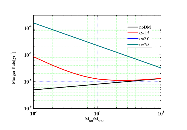
Figure 7: Same as Figure 5 but for NSCs.

As for the merger rate of GCs, we first need to assess the number of BHs in NSCs and to estimate the corresponding depletion timescale. We note that the total mass of an NSC is typically $100$ times that of the central IMBH (see Fig. 5 of Antonini et al., 2015). Following our earlier assumption that the average stellar- mass is $0.5M_{\odot}$, the stellar IMF is a Salpeter function, and only one-third of the newborn stellar BHs are retained, we find that the total number of BHs is $200$ for $M=1000M_{\odot}$, $2000$ for $M=10,000M_{\odot}$, and $20,000$ for $M=10^{5}M_{\odot}$.

With these numbers and not considering the effect of mass growth, we derive the duty cycles of BH mergers in NSCs, and the results are presented in Table 4. We find that the duty cycles are now comparable to one Hubble time when $M_{\rm BH}\geq 10^{4}M_{\odot}$. If we further consider the growth of IMBH due to the mergers, the duty cycles would be even longer because they are decreasing functions of $M_{\rm BH}$.

For those models that have a duty cycle shorter than one Hubble time, we need to consider BH depletion and the subsequent NS mergers. The merger rates are given in Table.(5) and illustrated in Figure 8. Because we find that NS merger rate could be much higher than that in GCs, we also need to consider the possibility of NS depletion. We estimate the total number of NSs in an NSC assuming that the stars in the mass range between $10M_{\odot}$ and $30M_{\odot}$ will turn into NSs. As a result, about $1$ percent of the initial stars would form NSs. Moreover, we assume that half the NSs, due to their large natal kicks, would escape from the NSCs. Then we find about $1000$ NSs for an IMBH of an initial mass $M_{\rm BH}=1000M_{\odot}$, $10^{4}$ for $M_{\rm BH}=10^{4}M_{\odot}$ and $10^{5}$ for $M_{\rm BH}=10^{5}M_{\odot}$. The resulting NS duty cycles are presented in Table 5.

Table 5: The merger rate of IMRIs/EMRIs with NSs for different dark matter density profiles in NSCs.

$M=3000M_{\odot}$	$\alpha=1.5$	$\alpha=2.0$	$\alpha=7/3$
Merger Rate	$8.0\times 10^{-9}\rm yr^{-1}$	$3.1\times 10^{-7}\rm yr^{-1}$	$1.2\times 10^{-6}$
Duty Cycle	$T_{\rm Hubble}$	$3.2\rm Gyr$	$8.3\times 10^{8}\rm yr$

$M=12,000M_{\odot}$	$\alpha=1.5$	$\alpha=2.0$	$\alpha=7/3$
Merger Rate	$6.2\times 10^{-9}\rm yr^{-1}$	$7.3\times 10^{-8}\rm yr^{-1}$	$3.8\times 10^{-7}\rm yr^{-1}$
Duty Cycle	$T_{\rm Hubble}$	$T_{\textrm{Hubble}}$	$T_{\rm Hubble}$

$M=21,000M_{\odot}$	$\alpha=1.5$	$\alpha=2.0$	$\alpha=7/3$
Merger rate	$6.6\times 10^{-9}\rm yr^{-1}$	$4.3\times 10^{-8}\rm yr^{-1}$	$2.4\times 10^{-7}\rm yr^{-1}$
duty cycle	$T_{\rm Hubble}$	$T_{\rm Hubble}$	$T_{\rm Hubble}$

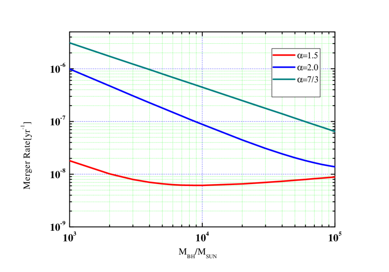
Figure 8: Same as Figure 5 but for IMBH-NS merger NSCs.

Figure 9 shows the final masses of IMBHs as a function of the initial ones. For those IMBHs that could deplete NSs during one Hubble time, the final masses include the contribution from all the stellar BHs and NSs in their host NSCs.

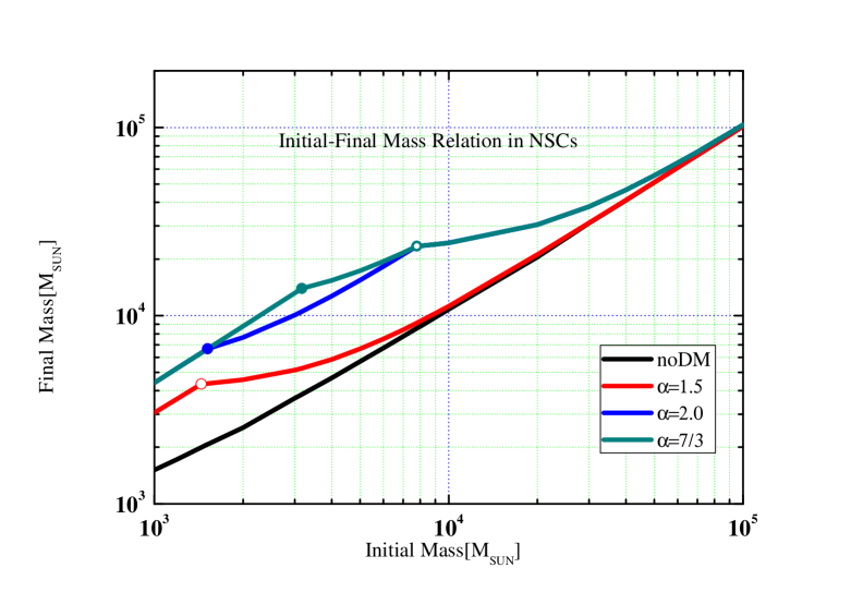
Figure 9: Same as Figure 6 but for the IMBHs in NSCs. The circles, at about $1500M_{\odot}$ when $\alpha=1.5$ and $7800$ when $\alpha=2.0$ and $7/3$, mark the masses with which a IMBH could deplete all the stellar BH in the same cluster. The solid dots are the masses corresponding to NS depletion, which is about $1500M_{\odot}$ when $\alpha=2.0$ and $3200M_{\odot}$ when $\alpha=7/3$.

4.2 Merger rate in nuclear star clusters per $\rm Mpc^{3}$

The calculation of the merger rate per unit ${\rm Mpc^{3}}$ for NSCs is almost the same as the previous calculation for GCs, but with two crucial modifications. (1) For the mass function of IMBHs, we consider two models. The first is suggested by Babak et al. (2017), which is

$$\frac{{\rm d}n}{{\rm d}\log M}=0.005\left(\frac{M}{3\times 10^{6}M_{\odot}}\right)^{-0.3}\rm Mpc^{-3}.$$ (27)

Another model, suggested by Gair et al. (2017), is more conservative,

$$\frac{{\rm d}n}{{\rm d}\log M}=0.002\left(\frac{M}{3\times 10^{6}M_{\odot}}\right)^{0.3}\rm Mpc^{-3}.$$ (28)

In this latter one, the exponent is positive, which significantly reduces the number of IMBHs. (2) When $\alpha\geq 2.0$, to calculate $\mathcal{R}_{\rm NS}$ the $M_{\rm min}$ in the integration of the mass function is determined by the solid dots in Figure 9, because smaller IMBHs in NSCs would have depleted all the NSs. The corresponding merger rates for BHs and NSs per $\rm Mpc^{3}$ are presented in Table6. Again, we find an enhancement of BH and NS merger rates in the presence of DM minispikes.

Table 6: The merger rate per $\rm Mpc^{3}$ of IMRIs or EMRIs with BHs $R_{\rm BH}$ and neutron stars $R_{\rm NS}$ formed by IMBH for different dark matter density profiles.

Barrause 12	no DM	$\alpha=1.5$	$\alpha=2.0$	$\alpha=7/3$
$R_{\rm BH}[\rm Mpc^{-3}{\rm yr}^{-1}$]	$1.0\times 10^{-9}$	$1.8\times 10^{-9}$	$4.3\times 10^{-9}$	$4.3\times 10^{-9}$
$R_{\rm NS}[\rm Mpc^{-3}{\rm yr}^{-1}$]	–	$1.4\times 10^{-10}$	$5.4\times 10^{-9}$	$8.7\times 10^{-9}$

Gair 10	no DM	$\alpha=1.5$	$\alpha=2.0$	$\alpha=7/3$
$R_{\rm BH}[\rm Mpc^{-3}{\rm yr}^{-1}$]	$1.7\times 10^{-11}$	$2.3\times 10^{-11}$	$8.9\times 10^{-11}$	$8.9\times 10^{-11}$
$R_{\rm NS}[\rm Mpc^{-3}{\rm yr}^{-1}$]	–	$5.1\times 10^{-13}$	$3.4\times 10^{-11}$	$7.4\times 10^{-11}$

From the calculations we can also find that the results are sensitive to the BH and NS supply. With DM minispike, the duty cycle of BHs and NSs may be shorter than the Hubble time, as the dramatically increased merger rate can lead to a high efficiency of consumption of compact objects. As a result, the appearance nowadays strongly depends on the total BH and NS supply.

5 Could stellar dynamics deplete the minispikes?

We have shown in Figures 1-3 that dynamical hardening, by ejecting intruding stars, is important for the initial evolution of IMRI/EMRIs, when $a>(10^{-3}\sim 0.1)$ pc. It is worth discussing here whether the same process could eject DM particles and hence deplete the DM minispikes.

The difference between hardening against DM and hardening against stars is that the interloper stars that we considered are gravitationally unbound to the IMBHs but the DM particles are deep in the potential well of the IMBH. The DM particles are more difficult to deplete. To show this more clearly, we calculate the hardening timescale associated with DM using the ejection timescale derived in Sesana et al. (2008) for the stars gravitationally bound to binary MBHs. They showed that it is $\tau=5P_{0}/q^{2}$, where $P_{0}$ is the orbital period of the binary. For example, the pink solid line in Figure 10 illustrates the dependence of this timescale on the IMBH mass.

The fact that the pink line is comparable or above the blue and green curves suggests that dynamical friction against DM is more efficient, so that the shrinking of the binary does not lead to the ejection of most DM particles, at least when $\alpha\geq 2$. In the case where $\alpha=1.5$, the hardening due to DM could be more efficient than the dynamical friction process, which implies that the shrinking of the binary could result in a depletion of the DM minispike. However, a DM minispike could also be replenished due to the self-interaction of DM particles or the adiabatic growth of the central IMBH(Peeebles, 1972),(Young., 1980),(Inpser et al., 1987),(Gondolo & Silk, 1999). Therefore, we conclude with caution that the merger rates calculated earlier in this paper are valid if DM minispike have steep profiles $\alpha\gtrsim 2$.

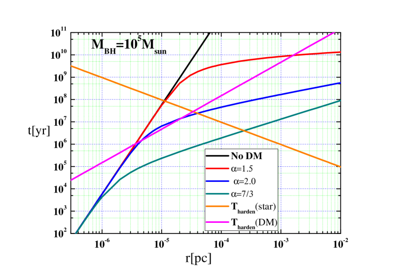
Figure 10: The same as Figure 3 but also showing the hardening timescale due to ejecting DM particles.

Another stellar dynamical effect that might potentially deplete the DM minispike is called "mass segregation". Such an effect normally leads to the formation of a dense cusp, composed of the heaviest stars in the cluster, around an IMBH (Bachcall and Wolf., 1976). If the cusp is mainly stellar BHs (single population), the density would follow a power-law distribution $\rho\propto r^{-7/4}$ (Bachall-Wolf cusp). In the conventional models of star clusters, such a cusp forms at the expense of repelling other less massive stars, as well as DM particles since they are also light in mass.

We think the effect of mass segregation is not important for most of our models because the region of our interest is normally very close to the central IMBH, so that very few stellar BHs would reach there. More precisely, according to Figures 1-3, the region where DM plays a crucial role in triggering the mergers is where we have $T<T_{\rm harden}$. If we define the critical radius where $T=T_{\rm harden}$ as $r_{\rm cri}$, and calculate the number of stellar MBH inside it, we find that the number is relatively small. For example, even if we consider a dense Bachall-Wolf cusp, the number of BHs inside $r_{\rm cri}$ would be

$$N(<r_{\rm cri})=\frac{1}{10M_{\odot}}\int_{0}^{r_{\rm cri}}n_{*}m_{\ast}(r/r_{\rm infl})^{-7/4}dr,$$ (29)

where $r_{\rm infl}=GM/\sigma^{2}$ is the influence radius of the central IMBH, and $n_{*}$ is the number density of stars as in Section 3. Then we find that given the $M_{\rm BH}$ of our interest, the number of stellar BHs inside $r_{\rm cri}$ is $\leq 1$ when $\alpha=1.5$. When $\alpha=2.0$, this number becomes $\sim 0.5$ for $M=1000M_{\odot}$, $\sim 1$ for $M=10^{4}M_{\odot}$, and $\sim 6$ for $M=10^{5}M_{\odot}$.When $\alpha=7/3$, the number is $\sim 2$ for $M=1000M_{\odot}$, $\sim 15$ for $M=10^{4}M_{\odot}$, and $\sim 48$ for $M=10^{5}M_{\odot}$.

Therefore, it seems that only when $\alpha=7/3$ dose the effect of mass segregation become relevant. However, even in this case, if we further compare the timescale for the Bachall-Wolf cusp to regrow and the timescale for the stellar BHs to merger with the central IMBH ($T$ in the previous sections), we find that the latter timescale is typically shorter. For example, according to Equation (17), the growth timescale for the cusp is $3\times 10^{5}\rm yr$ for $M=1000M_{\odot}$, $2\times 10^{6}\rm yr$ for $M=10^{4}M_{\odot}$ and $1.5\times 10^{7}\rm yr$ for $M=10^{5}M_{\odot}$. They are shorter than the merger timescales as shown in Figures 1, 2, and 3. This result indicates that the Bachall-Wolf cusp cannot form in the case of $\alpha=7/3$, so that we do not need to consider the effect of mass segregation on the depletion of DM minispikes.

6 Conclusions

In this paper we study the effect of DM minispikes around IMBHs on the merger rate of IMRIs and EMRIs. We considered IMBHs with a mass between $10^{3}M_{\odot}$ and $10^{5}M_{\odot}$, as well as three typical density profiles for the DM, namely $\alpha=1.5$, $2.0$, and $7/3$.

We find that the presence of DM minispikes significantly reduces the merger timescale of EMRIs and IMRIs due to the effet of dynamical friction. The effect is more significant for small IMBHs ($<10^{4}M_{\odot}$) with steep DM density profiles $\alpha\geq 2.0$, and in the most extreme case the shortening of the timescale can be two to three orders of magnitude.

As a result, the merger rate of stellar-mass BHs with IMBH in a cluster is enhanced by as much as two orders of magnitude, to a degree that all the BHs in the cluster are exhausted. After the BHs are depleted, the mergers with NSs would become important and dominate the current event rate of IMRIs/EMRIs.

The enhancement of the merger rate also modifies the mass function of IMBHs because they can grow a significant amount of mass during one Hubble time. This effect is important for the IMBHs with a mass of $\lesssim 10^{4}M_{\odot}$ and we derived the final mass function in this mass range according to our model.

We conclude that the presence of DM around IMBHs would significantly change the event rate of IMRIs and EMRIs, The effect is not necessarily an enhancement of the merger rate because stellar-mass BHs could be exhausted and the subsequently IMRI/EMRI events are dominated by the mergers with NSs. On the other hand, in the absence of DM minispikes, we predict that there are almost no mergers of IMBHs with NSs.

The above predictions can be tested in the future by space-based GW detectors, such as LISA, Taiji, and Tianqin. These future observations will allow us to better understand the DM physics, the formation and evolution of IMBHs, as well as and stellar dynamical processes in GCs and NSCs.

References

- Amaro-Seoane et al. (2013) Amaro-Seoane P., Aoudia S. , Audley H. et al. 2013, arXiv1305.5720E.
- Amaro-Seoane et al. (2017) Amaro-Seoane P., Audley H., Babak S. et al. 2017, arXiv170200786A.
- Amaro-Seoane et al. (2009) Amaro-Seoane P., Eichhorn P., Porter E. K., and Spurzem R., 2009, MNRAS, 401, 2268.
- Antonini et al. (2015) Antonini F., Barausse E. and Silk J., 2015,arXiv:1506.02050,Accepted for publication in ApJ.
- Bachcall and Wolf. (1976) Bahcall J. N., and Wolf R. A., 1976, ApJ, 209, 214.
- Babak et al. (2017) Babak S., Gair J., Sesana A., Barausse E., Sopuerta C. F., Berry C. P. L., Berti E., Amaro-Seoane P., Petiteau A., 2017, KleinPhys A., Rev. D; 95:103012.
- Baldry et al. (2008) Baldry IK, Glazebrook K, Driver SP. 2008. MNRAS 388:945
- Bertone et al. (2005) Bertone G. and Merritt D., 2005, Phys. Rev.D 72,103502.
- Bertone et al. (2005) Bertone G., Zentner A. R., and Silk J., 2005, Phys. Rev. D 72,103517.
- Bik et al. (2003) Bik, A., Lamers, H. J. G. L. M., Bastian, N., Panagia, N., & Romaniello, M. 2003, A&A, 397, 473
- de Grijs et al. (2003) de Grijs, R., Anders, P., Bastian, N., Lynds, R., Lamers, H. J. G. L. M., & O’Neil, E. J. 2003, MNRAS, 343, 1285
- Eda et al. (2013) Eda K., Itoh Y., Kuroyanagi S., Silk J., 2013, Phys. Rev. Lett. 110, 221101.
- Eda et al. (2015) Eda K., Itoch Y., Kuroyanagi S., and Silk J., 2015, Phys. Rev. D 91, 044045.
- Ferrer et al. (2017) Ferrer F., da Rosa A. M., Will C. M., 2017, Phys. Rev. D 96, 083014.
- Feng & Soria (2011) Feng H., Soria R., 2011, New Astro. Rev. 55, 166.
- Farrel et al. (2009) Farrel S. A., Webb N. A., Barret D., Godet O., and Rodrigues J. M., 2009, Nature, 460, 73.
- Farrel et al. (2010) Farrell S. A., Servillat M., Oates S. R., et al. 2010, X-ray Astronomy.
- Gondolo & Silk (1999) Gondolo P. and Silk J., 1999, Phys. Rev. Lett. 83, 1719 .
- Gair et al. (2017) Gair J. R, Babak S., Sesana A., Amaro-Seoane P., Barausse E., Berry C. P. L., Berti E., Sopuerta C., arXiv:1704.00009.
- Gnedin et al. (2014) Gnedin, O. Y., Ostriker, J. P., & Tremaine, S. 2014, ApJ, 785, 71 .
- Gómez & Rueda, (2017) Gómez L. G., Rueda J. A., 2017, Phys. Rev. D, 96, 063001
- Gong et al. (2011) Gong X., Xu S., Bai S. et al., 2011, Class. Quant. Grav. 28, 094012.
- Gürkan et al. (2006) Gürkan M. A., Fregeau J. M., Rasio F. A., 2006, ApJ, 640, L39.
- Gültekin et al. (2009) Gültekin, K., Richstone, D. O., Gebhardt, K., et al. 2009, ApJ, 698, 198
- Heggie (1975) Heggie D.C.,1975,MNRAS,173.729H.
- Kruijssen (2012) Kruijssen, J. M. D. 2012, MNRAS, 426, 3008
- Matsubayashi et al (2007) Matsubayashi, T., Makino, J., & Ebisuzaki, T. 2007, ApJ, 656, 879.
- Merritt et al. (2002) Merritt D., Milosavljevic M., Verde L., and Jimenez R., 2002, Phys. Rev. Lett.88, 191301.
- Merritt (2004) Merritt D., 2004, Phys. Rev. Lett.92,201304.
- Inpser et al. (1987) Ipser J. R. and Sikivie P., 1987, Phys. Rev. D 35, 3695.
- Luo et al. (2016) Luo J., Chen L.-S., Duan H.-Z. et al., 2016, Class. Quant. Grav. 33,035010.
- Miller & Hamilton (2002) Miller M. C., and Hamilton D. P., 2002, MNRAS, 330, 232.
- Mandel et al. (2008) Mandel I., Brown D. A., Gair J. R. and Miller M. C., 2008, ApJ. 681,1431.
- Navarro et al. (1997) Navarro J. F., Frank C. S., and White S. D. M., 1997, Astrophys.J. 490, 493.
- Peeebles (1972) Peebles P. J. E.,1972, Astrophys. J. 178, 371.
- Phillips et al. (1996) Phillips, A. C., Illingworth, G. D., MacKenty, J. W., & Franx, M. 1996, AJ, 111, 1566
- Peters & Mathews (1963) Peters P. C. and Mathews J., Physical Review 131, 435 (1963).
- Pryor & Meylan (1993) Pryor C., and Meylan G., 1993, in ASP Conf. Ser. 50, Structure and Dynamics of Globular Clusters, ed. Djorgovski S. G. and Meylan G. (San Francisco: ASP), 357.
- Quinian et al. (1995) Quinian G. D., Hernauist L., and Sigurdsson S., 1995, ApJ. 440, 554.
- Quinlan (1996) Quinlan C. D., 1996, New Astronomy, 1, 35.
- Rodríguez et al, (2017) Rodríguez J. F., Rueda, J. A. Ruffini, R. 2018, JCAP 02, 030.
- Sesana et al. (2008) Sesana A., Haardt F., Madau P., 2008, ApJ, 686, 432.
- Ullio et al. (2001) Ullio P., Zhao H. S., and Kamionkowski M., 2001, Phys. Rev. D 64, 043504.
- Walcher et al. (2005) Walcher, C. J., van der Marel, R. P., McLaughlin, D., et al. 2005, ApJ, 618, 237
- Young. (1980) Young. P. 1980, ApJ, 242,1232.
- Yue & Han (2018) Yue X-J. and Han W-B., 2018, Phys. Rev. D, 97, 064003.
- Zhao & Silk (2005) Zhao H. S. and Silk J., 2005, Phys. Rev. Lett. 95,011031.