The Spectrum of the Universe
Abstract
The cosmic background (CB) radiation, encompassing the sum of emission from all sources outside our own Milky Way galaxy across the entire electromagnetic spectrum, is a fundamental phenomenon in observational cosmology. Many experiments have been conceived to measure it (or its constituents) since the extragalactic Universe was first discovered; in addition to estimating the bulk (cosmic monopole) spectrum, directional variations have also been detected over a wide range of wavelengths. Here we gather the most recent of these measurements and discuss the current status of our understanding of the CB from radio to -ray energies. Using available data in the literature we piece together the sky-averaged intensity spectrum, and discuss the emission processes responsible for what is observed. We examine the effect of perturbations to the continuum spectrum from atomic and molecular line processes and comment on the detectability of these signals. We also discuss how one could in principle obtain a complete census of the CB by measuring the full spectrum of each spherical harmonic expansion coefficient. This set of spectra of multipole moments effectively encodes the entire statistical history of nuclear, atomic and molecular processes in the Universe.
1 Introduction
If you look at the sky with relatively wide angular resolution, concentrating on radiation coming from beyond Earth’s atmosphere, past the Solar System and outside the Milky Way galaxy, you would only see diffuse anisotropies on top of a homogeneous, isotropic background. This is known as the “cosmic background” (CB). The sources contributing to this background can range from astronomically small objects, such as atoms, nuclei and dust grains, to stars, galaxies and galaxy clusters, and are created by processes like nuclear fusion, gravitational collapse and thermal radiation. As the CB is composed of photons ranging from hundreds of thousands to nearly fourteen billion years old, its all-sky energy encodes the history of structure formation, energy distribution and expansion in the Universe. It is an important tool in cosmology today, and a huge amount of effort has been put into measuring, interpreting and predicting its spectrum.
The CB can be observed over some 17 orders of magnitude in frequency ( to Hz), which has required a plethora of detection techniques to measure and many different theoretical models to interpret, hence we tackle this by splitting the spectrum into sections, or wavebands. Astronomers traditionally work in radio, microwave, infrared, optical, ultraviolet, X-ray and -ray wavebands, each section unique in its radiation detection methods, units and jargon, although the same physical quantity (namely the isotropic photon background) is being described. To construct the entire CB it will therefore be necessary to perform a survey across effectively the whole astronomical discipline and to understand exactly how each measurement has been made, while translating the results into something mutually comparable.
Historically (Trimble, 2006), the study of the CB took off in earnest with the discovery of the diffuse microwave component in 1965 (Penzias & Wilson, 1965; Dicke et al., 1965), although the first cosmic sources of X-rays were known slightly earlier than that (Giacconi et al., 1962) and distant radio sources had been detected a couple of decades earlier still, although their interpretation was a long and complicated story (see e.g. Sullivan, 2009, for a review), with direct detections of the radio background coming in the late 1960s (Bridle, 1967). Moreover, it had been known since the early 20th century that we could see optical photons from well beyond our own Galaxy. Emission from the Galaxy is highly anisotropic, being concentrated into a band across the sky (the Milky Way), which is visible in many wavebands. The study of our own Galaxy, and the objects within it, is of course an interesting topic in its own right, but here we are focusing on more distant (‘cosmic’ or ‘cosmological’) radiation, and so we assume that the Galactic contributions have been removed.
Efforts to gather the necessary data into one coherent survey of the CB were first carried out by Longair & Sunyaev (1972). At that time, the shape of the background spectrum was largely speculative, with only a few rough measurements available in selected wavebands, along with upper limits at other wavelengths and theoretical ideas for what the backgrounds might be from various physical processes. Other studies tended to focus on one part of the electromagnetic spectrum, but about 20 years after Longair & Sunyaev’s seminal work, Ressell & Turner (1990) compiled an updated plot of the background intensity, showing the dramatic progress that had already been made. Rather than constructing their plot mostly from theoretical considerations, Ressell and Turner had enough physical data available to them that they could simply convert the units and put all the empirical information together. Though a significant improvement on what had come before, their work showed that there was still much uncertainty at key wavelengths. These results were later updated by Scott (2000), and there have also been various compilations focusing on individual wavebands of the background, primarily in the optical/infrared (e.g., Longair, 2001; Hauser & Dwek, 2001; Lagache et al., 2005; Driver et al., 2016), and the X-ray/-ray (e.g., Boldt, 1987; Fabian & Barcons, 1992; Hasinger, 1996; Bowyer, 2001; Ajello et al., 2015) regimes, or carried out in the context of modelling studies (e.g., Bond et al., 1986; Gilli et al., 2007; Franceschini et al., 2008; Finke et al., 2010; Gilmore et al., 2012; Khaire & Srianand, 2018). These earlier CB studies either include measurements that are now quite out of date, or lack information from the wider range of frequencies available. Some other recent reviews cover a range of wavelengths, but are less comprehensive than this one (e.g., Dwek & Krennrich, 2013; Cooray, 2016; Franceschini & Rodighiero, 2017).
Because of the numerous applications of the CB in astronomy, astrophysics and cosmology, it is useful to compile an up-to-date picture of its intensity distribution. Here we combine the most recent published data in order to present a single, coherent plot of the background radiation spectrum. At the same time we explore some implications coming from picking apart the constituents of this spectrum. We will begin in Section 2 with a brief discussion of what it means to measure the CB, what units are commonly adopted and various conversion factors between them. In Section 3 we present the sky-averaged CB intensity in the different wavebands, and discuss some of the emission processes responsible for the observed features. In Section 4 we discuss perturbations to the CB contiuum spectrum from line emission processes, while in Section 5 we consider a more complete picture of the background sky by considering higher-order multipole moments. We summarize our results in Section 6. Our goal is to present the current status of the spectrum of the Universe, along with a summary of our understanding of its origin and the implications it has for astrophysics and cosmology.
2 Units and definitions
It is first necessary to define exactly what we mean by the CB. A measurement of background radiation sounds rather ambiguous. Where was the telescope pointed? What do we do about anisotropies? What about units? Larger detectors and bandwidths will receive more energy per second, larger beamwidths will see more of the sky simultaneously, so how do we interpret the numbers?
2.1 Units
We will report our findings in SI units of frequency in hertz and specific intensity in W m-2 sr-1 Hz-1. This is the power a detector would receive per unit area, per solid angle observed on the sky, per unit frequency of light being detected. So, for example, multiplying by (the solid angle of the entire sky) and by the area of a detector’s surface and its frequency bandwidth would give the amount of power that an ideal detector receives.
It is convenient to multiply by because gives the contribution per unit logarithmic scale. In addition, since is proportional to the energy density per unit frequency, plotting will give a qualitative view of how the energy density is distributed across the spectrum. In other words, if two features have equal width in , then the one that is higher in contains more energy density.
In the astronomical literature units vary wildly between waveband specializations. Here we give some key conversion factors necessary to obtain the desired intensity unit, W m-2 sr-1 Hz-1.
2.1.1 Frequency
Frequency, wavelength and energy are all interchangeable. The wavelength is extensively used when discussing microwave through ultraviolet frequencies, but for radio waves the frequency tends to be used, and when it comes to high-energy photons frequency is usually expressed as photon energy . We convert wavelength to frequency via
| (1) |
where is the speed of light, and we convert energy to frequency with
| (2) |
where is Planck’s constant. One also sometimes encounters the wavenumber, which is the frequency given in inverse length units
| (3) |
2.1.2 Intensity
If the specific intensity per unit wavelength is , we need to use
| (4) |
to convert to specific intensity per unit frequency.
In radio astronomy, it is common to find the specific intensity given as a “brightness temperature” , which is defined as the temperature of a perfect blackbody emitting at the observed intensity in the Rayleigh-Jeans (i.e., low energy) regime, i.e.,
| (5) |
where is the Boltzmann constant.
Low-energy astronomers also like to use the jansky (Jy) to represent specific flux (which is the specific intensity integrated over the solid angle of the region in the sky of interest), where
| (6) |
2.1.3 Energy
The erg is a commonly used quantity in several sub-branches of astronomy, while in high-energy astronomy energy is generally given in electron-volts (eV). In order to convert ergs to joules we use
| (7) |
and in order to convert electron-volts to joules we use
| (8) |
where is a unitless number whose magnitude is the electron charge.
2.1.4 Solid angle
For measuring radiation coming from the sky the solid angle is important. This is often given in square degrees, , which can be converted to steradians through
| (9) |
2.2 Redshift
In cosmology, distances are frequently referred to in terms of “redshift”. The redshift of a source is a measure of how much the observed wavelengths are stretched by the expansion of the Universe:
| (10) |
Here is the frequency of a photon that has been emitted by the source, and is the frequency that same photon is observed to have on Earth.
The evolutionary history of redshift, or equivalently expansion, is governed by the now conventional vacuum-energy (or ) dominated cold dark matter (CDM) model, in which the Universe is flat on cosmological scales, the energy density of the Universe is composed of (mostly cold dark) matter and vacuum energy with fractions and , respectively, and the local expansion rate per unit length is (Planck Collaboration XIII, 2016). Because the expansion is so well understood, a measurement of the spectral shift of a source tells us how distant the source is through a monotonic function:
| (11) |
Redshifts are relatively easy to measure (from spectral lines) and then distances are determined using the above equation. As a result of the finite speed of light, distant objects are observed as they were long ago. Because of this, cosmologists use redshift as a proxy for both distance and cosmic epoch.
2.3 Spherical harmonics
In general we could describe the sky by giving the spectral intensity in every direction. The natural way to do this is to decompose the sky into spherical harmonics, i.e., the specific intensity as a function of polar angle and azimuthal angle can be written as
| (12) |
where are the usual spherical harmonics.
Each term in the expansion has a physical meaning. Noting that , it follows that is just the intensity averaged over the sky. The three terms () are related to the dipole moment of the intensity. For large , the th components of the spherical harmonic expansion correspond to the intensity contribution from angular scales of approximately .
In what follows, we will be looking at the term, i.e., the average value of the intensity per unit frequency in the sky, after subtraction of all the light from the Milky Way, our Solar System and the atmosphere. This gives the average spectrum of radiation from the extragalactic Universe. We shall return to a discussion of angular dependence later – but it is worth noting for now that since the Universe is close to homogeneous on large scales then any deviations from the average spectrum are relatively small.
2.4 Dividing the CB
As we have previously mentioned, it is convenient to split the electromagnetic spectrum into sections. Following astronomical convention, these are the radio, microwave, infrared, optical, ultraviolet, X-ray and -ray waveband ranges; as such, we will denote the various sections of the CB as the cosmic radio, microwave, infrared, optical, ultraviolet, X-ray and -ray backgrounds, or the CRB, CMB, CIB, COB, CUB, CXB and CGB, respectively. Table 1 lists these ranges in units of frequency, wavelength and energy.
| Part of CB | Frequency range | Wavelength range | Energy range |
|---|---|---|---|
| Cosmic radio background (CRB) | Hz | mm | 40eV |
| Cosmic microwave background (CMB) | –Hz | 0.3–30 mm | 0.04–4 meV |
| Cosmic infrared background (CIB) | –Hz | 3–300m | 4–400 meV |
| Cosmic optical background (COB) | –Hz | 0.3–3m | 0.4–4 eV |
| Cosmic ultraviolet background (CUB) | –Hz | 30–300 nm | 4–40 eV |
| Cosmic X-ray background (CXB) | –Hz | 0.03–30 nm | 0.04–40 keV |
| Cosmic -ray background (CGB) | Hz | 0.03 nm | keV |
3 The cosmic background
We are now in a position to discuss the spectrum of the Universe. We will go over each division of the CB in some detail, discussing which physical processes are contributing to each frequency range and presenting the current estimates of from available data. We will also describe some of the measurement approaches that are used to constrain the CB spectrum. Most astronomical imaging experiments are not sensitive to the average value of the image; in other words they are effectively differential measurements, which cannot directly determine the monopole amplitude. There are some absolute measurements of the amplitude of the CB, but these are the exception, and, as we will see below, most determinations are more indirect.
3.1 The cosmic radio background (CRB)
[Hz, mm]
The radio portion of the spectrum includes all frequencies below around Hz. The current theoretical picture of the CRB is that it is mainly the sum of synchrotron emission emitted by charged particles moving through diffuse galactic and inter-galactic magnetic fields, along with emission from active galactic nuclei (AGN) and Hi line emission, combined with the low energy end of the CMB (Singal et al., 2010). The energy released by synchrotron radiation is proportional to the square of the magnetic field strength, but since magnetic fields on the scales of galaxies are quite small (of order T, e.g., Widrow, 2002), the photons emitted have relatively low energies (see Section 3.2 for details on the CMB contribution).
There is a lower limit to the frequencies of the CRB that we can observe due to the plasma frequency of the Earth’s atmosphere and our Milky Way Galaxy, given by
| (13) |
where is the electron number density and the electron mass. This frequency is the rate at which free electrons in a plasma oscillate; if the frequency of a propagating electromagnetic wave is less than the plasma frequency, it will be exponentially attenuated on scales much shorter than the wavelength (Chabert & Braithwaite, 2011). The Earth’s ionosphere has a plasma frequency on the order of 10 MHz, limiting all ground based observations of the CRB, while the interstellar medium (ISM) has a plasma frequency of about 1 MHz, limiting even space-based observations (Lacki, 2010).
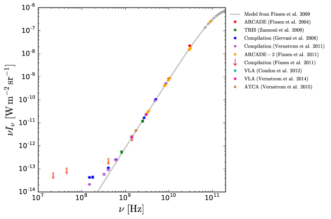
The data in this waveband come from a combination of ground and balloon-borne instruments. In our compilation (see Fig. 1) we include measurements of the absolute intensity of the sky from the Absolute Radiometer for Cosmology, Astrophysics and Diffuse Emission (ARCADE) experiment (Fixsen et al., 2004) and its successor, ARCADE-2 (Fixsen et al., 2011), which measured the CRB between 3 and 90 GHz by subtracting a model of Galactic emission. Also reported by these authors are four absolute measurements performed between 1980 and 1990 at 0.022, 0.045, 0.408 and 1.42 GHz, to which the same Galactic foreground model was subtracted to obtain the CRB. We consider the latter four measurements as upper limits because these observations were taken much closer to the Galactic plane than later dedicated background experiments.
In addition, the TRIS experiment, a set of three ground based radiometers, measured the CRB at 0.6, 0.8 and 2.5 GHz (Zannoni et al., 2008). We also use two studies that employed a compilation of radio galaxy counts to estimate the total value of the CRB (Gervasi et al., 2008; Vernstrom et al., 2011, and references therein). We give further derived detections of the CRB obtained with the Karl G. Jansky Very Large Array (VLA) at 1.4 and 3 GHz (Condon et al., 2012; Vernstrom et al., 2014) and by the Australian Telescope Compact (ATCA, Vernstrom et al., 2015) at 1.75 GHz.
The values we report here were converted from brightness temperature (see Eq. 5). We note that the CRB value reported by Vernstrom et al. (2011) includes only the contribution from galaxies (and would have missed any genuinely diffuse emission). It is therefore necessary to add the CMB temperature, experimentally found to be K (Fixsen, 2009, as discussed in the next sub-section), to obtain the total intensity.
Figure 1 shows the CRB (i.e., the CB at radio frequencies). For comparison, we have plotted the low-energy end of a blackbody spectrum with temperature . We can see very good agreement in the shape of the curve with that of a blackbody over much of the radio region, and as expected, at lower frequencies the data lie slightly higher due to the contributions from galaxies. There is some debate regarding the robustness of the excess radiation seen by the ARCADE-2 experiment (e.g., Subrahmanyan & Cowsik, 2013), in particular at the higher frequencies. Subtracting from the brightness temperatures obtained from each experiment shows that ARCADE-2 obtained excess values that were significantly higher than those observed by TRIS or those calculated via galaxy counts (see Vernstrom et al. 2011 and Singal et al. 2017 for more detailed discussions).
3.2 The cosmic microwave background
(CMB)
[–Hz,
–30 mm]
The CMB is dramatically the highest amplitude part of the CB. It is also the most thoroughly studied portion of the spectrum (possibly the most thoroughly studied phenomenon in cosmology), and its origin is now very well understood. The CMB is the blackbody radiation left over from the hot early phase of the Universe. It was last scattered by matter about 400,000 years after the Big Bang, when the temperature cooled enough to allow protons to combine with electrons and form neutral atoms, transforming the Universe from optically thick to optically thin. The temperature of the Universe at this time was about 3000 K. Today we see the temperature to be 2.7255 K, owing to the fact that scales have redshifted by a factor of about 1100 since the last-scattering epoch (see e.g., Scott & Smoot, 2016). A great deal of physics can be discerned from studying the possible spectral distortions and spatial variations (or anisotropies) in the CMB (e.g., Samtleben et al., 2007). These anisotropies currently provide the tightest constraints on the parameters that statistically describe our Universe (Planck Collaboration XIII, 2016).
Blackbody radiation from the CMB follows the Planck intensity function,
| (14) |
For a blackbody with K, the peak (in ) is at about GHz, or mm. Given the precise mathematical form of this part of the CB, we can integrate to obtain the energy density of the CMB, J m eV cm-3, or the number density of CMB photons, cm-3.
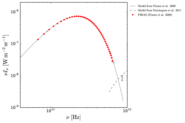
The CMB spectrum has been measured to great precision by the Far InfraRed Absolute Spectrophotometer (FIRAS) instrument aboard the COsmic Background Explorer (COBE) satellite (Fixsen et al., 1996), with a spectrum shown to be very close to that of a blackbody. There are also earlier measurements that have provided a useful supplement to those from COBE-FIRAS, particularly at lower frequencies (e.g., Halpern et al., 1988; Gush et al., 1990; Mather et al., 1990; Levin et al., 1992; Staggs et al., 1996, as well as those in the radio, as already discussed); however, we have not incorporated these into our analysis, since the measurements from FIRAS span the same frequency range and provide smaller error bars. On the high frequency side, additional measurements at high resolution provide estimates of the resolved (i.e., broken up into discrete sources) fraction of the background at sub-millimetre wavelengths, and in particular, recent observations using the Atacama Large Millimeter/sub-millimeter Array (ALMA) have resolved close to 100 of the CMB-subtracted background into extragalactic sources (Carniani et al., 2015; Fujimoto et al., 2016; Aravena et al., 2016). However, due to the fact that the contribution to the CMB from extragalactic sources is several orders of magnitude smaller than the thermal radiation leftover from the Big Bang, we have not incorporated these measurements into our compilation.
The CMB measurements from FIRAS are plotted in Fig. 2, along with a blackbody function (Eq. 14) with a temperature of . Error bars are present, but in many cases are much smaller than the points themselves. Agreement between the measurements and a Planck spectrum is one of the strongest pieces of evidence for the hot Big Bang model, since the photon spectrum is expected to naturally relax to a state of thermal equilibrium in a model in which the early Universe was hot and dense; there is no other explanation for this nearly perfect blackbody shape.
3.3 The cosmic infrared background (CIB)
[–Hz,
–300 m]
The CIB contains approximately half of the total energy density of the radiation emitted by stars through the history of the Universe (although with roughly a factor of 40 less total energy density than contained in the CMB) and is tightly linked to the history of galaxy formation. This radiation is primarily emitted by dust that has been heated by the stars contained within galaxies (e.g., Lagache et al., 2005). At the long wavelength end we see the energy output of the oldest, most redshifted galaxies, which are key to understanding the beginnings of galaxy evolution.
This portion of the CB is extremely difficult to measure through absolute intensity measurements. Objects in our Solar System (such as planets, asteroids and dust) contribute a huge amount of unwanted ‘zodiacal’ emission, and dust emission from our own Milky Way Galaxy provides orders of magnitude of foreground emission to subtract from the measurements (e.g., Whittet, 1992). One approach to deal with this difficulty is to count the number of resolvable galaxies and measure their flux, extrapolate the data to take into account fainter undetected sources, then sum over the whole sky (as was done by Vernstrom et al., 2011, with radio galaxies). This gives a lower estimate, since it deals with only the contributions to the CIB from individually identified sources. Upper bounds, on the other hand, can be obtained through an entirely different approach. The spectra of -ray-emitting objects (such as a particular class of AGN called “blazars”) should have a deficit of high-energy photons, which interact with low energy CIB photons via pair production (see de Jager & Harding, 1992, for details). However, such upper limits depend of how the intrinsic spectra of blazars are modelled, as well as details of the distribution of sources responsible for producing the CIB photons, and hence there is not complete agreement on how tight the limits are. With these complications in mind we will report only a few representative results on upper or lower bounds to the CIB.
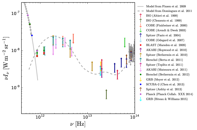
In the far- to mid-IR range (comprising 500–100 m) we use measurements taken by adding up sources detected by the Herschel Space Observatory’s Photodetector Array Camera and Spectrometer (PACS, Berta et al., 2011) and Spectral and Photometric Imaging REceiver (SPIRE, Béthermin et al., 2012), and the Balloon-borne Large Aperture Submillimeter Telescope (BLAST, Marsden et al., 2009). There have also been estimates of the CIB at 450 and 850 m made using the Submillimeter Common-User Bolometer Array-2 (SCUBA-2), a camera mounted on the James Clerk Maxwell Telescope (JCMT, Chen et al., 2013). In addition, we include two absolute measurements of the CIB at 140 and 240 m, made with the Diffuse InfraRed Background Experiment (DIRBE) aboard COBE (Odegard et al., 2007). We also have estimates using galaxy counts from the Far-Infrared Surveyor (FIS) aboard the Akari satellite at 65, 90, 140 and 160 m (Matsuura et al., 2011), and more recently from the Planck satellite between 350 and 1400 m (Planck Collaboration XXX, 2014). The CIB values determined in most of these papers had the CMB subtracted, since the scientific motivation was to study excess intensity over the CMB blackbody as opposed to the total intensity; for our purposes we have added a blackbody with back into the results.
Moving on to the mid-infrared (100–5 m), further analyses of DIRBE data at 4.9 m, and at 60 and 100 m by Arendt & Dwek (2003) and Finkbeiner et al. (2000), respectively, have yielded more robust background estimates than the earlier studies. Additionally, the Spitzer Space Telescope was used to observe the infrared sky at 3.6, 4.5, 5.8 and 8.0 m with the InfraRed Array Camera (IRAC), from which the CIB intensity was estimated by summing up detected sources (Fazio et al., 2004; Ashby et al., 2013). The Multiband Imaging Photometer for Spitzer (MIPS), with wavebands centred at 24, 70 and 160 m, was used in a similar fashion to obtain additional CIB measurements (Béthermin et al., 2010). Spitzer’s final instrument, the InfraRed Spectrograph (IRS), was employed by Teplitz et al. (2011) to estimate the CIB at 16 m. To fill in the gap between IRAC and MIPS, we present further CIB lower estimates from the Infrared Space Observatory ISOCAM at 7, 12 and 15 m (Altieri et al., 1999; Clements et al., 1999), and Akari’s InfraRed Camera (IRC, Hopwood et al., 2010).
Upper bounds found from -ray spectra of blazars have been derived using many different observations and detailed modelling approaches. Here we are primarily interested in obtaining upper limits in the mid-IR range, where dust contamination prevents absolute measurements from being obtained. For this, Meyer et al. (2012) derived an upper limit of 24 at 8 m, while Biteau & Williams (2015) obtained a limit of 16 at 16 m. There are many other -ray-derived background limits that could be used (e.g., Dwek & Krennrich, 2013), but for the sake of clarity we will only include the two above.
The total CIB is shown in Fig. 3, with the CMB blackbody shown again for comparison. There have been many attempts to build models for the infrared/optical background. We have plotted one example of such models, which was constructed by adding up the spectral energy distributions of a set of galaxy types, weighted by appropriate fractions (Domínguez et al., 2011). There is a clear local maximum here, despite the constraints only coming from upper and lower bounds in some regions. The peak lies at around 2– Hz (100–150 m) and contains an energy density of approximately .
3.4 The cosmic optical background (COB)
[–Hz,
–3 m]
The optical background is perhaps the second most important portion of the CB (at least for beings with eyes like ours) after the CMB, since it is dominated by the emission coming directly from stars. From this radiation we can infer much about the history of cosmic star formation. Because of this, it is a highly studied region of the CB – in addition to the fact that astronomy has traditionally been dominated by optical wavelengths, driven by the fact that ground-based telescopes can easily study optical photons.
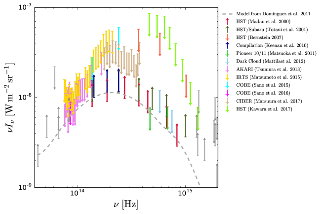
Since the Milky Way’s dust emission continues to be a confusing foreground well into optical wavelengths, direct estimates of the COB are also challenging. The best measurements tend therefore to be sums over sources. For instance, Madau & Pozzetti (2000) achieved lower bounds on the COB with the Hubble Space Telescope’s (HST) Hubble Deep Field survey in seven optical bandpasses (0.36–2.2 m) by counting galaxies. In addition, Totani et al. (2001) included in the galaxy counts sources observed in the Subaru Deep Field by the ground-based Subaru Telescope. An attempt to obtain absolute background estimates using HST observations between 0.3 and 0.8 m was carried out by Bernstein (2007), and more recently between 0.2 and 0.7 m by Kawara et al. (2017), which we treat here as upper limits. Lastly, Keenan et al. (2010) calculated the COB contribution from galaxies using galaxy counts from a wide range of studies dating back to 1999 (including their own observations in the near-IR band with Subaru).
There have been many additional attempts to determine the COB spectrum via direct detection, i.e., by attempting to subtract Galactic and zodiacal emission from rocket or satellite data. We have taken data obtained by the IRC mounted aboard the Akari satellite (Tsumura et al., 2013) and by the Near Infra-Red Spectrometer (NIRS) on the InfraRed Telescope in Space (IRTS, Matsumoto et al., 2015), each of which was designed to study 1.5–4.0 m radiation. More recently than these experiments was the Cosmic Infrared Background Explorer (CIBER), primarily designed to measure fluctuations around 1 m, but which provided an estimate of the averaged power using models of the fractional level of fluctuations (Matsuura et al., 2017). There has also been renewed interest in eliminating systematic effects from the DIRBE observations; re-analyses were performed at 1.25, 2.2 and 3.5 m (Sano et al., 2015, 2016). A further approach to remove zodiacal contamination involved using background light measurements from Pioneer 10 and 11 Imaging Photopolarimeter (IPP) data (Matsuoka et al., 2011); the instruments observed the sky when the spacecraft were about 5 AU from the Sun, where zodiacal light contributions were smaller. Lastly, we incorporate a measurement at 400 and 520 nm using the “dark cloud” technique (Mattila et al., 2012), where the difference in intensity between a high latitude dark nebula and its surroundings is taken to be solely due to the COB.
These results are combined in Fig. 4. Following the trough seen in the CIB, there is another peak here at about Hz (1 m), containing a similar total energy density to that from the CIB peak (i.e., around ). There is some tension between the lower limits from galaxy counts, the “dark cloud” measurement and the analysis of Pioneer 10 and 11 data. Systematic effects are difficult to control in direct measurement techniques, and it seems likely that the estimates from galaxy counts are close to the true background levels. We also show in Fig. 4 the model from Domínguez et al. (2011), which carries over to optical frequencies. In 2002 a similar study, adding up the spectra of 200,000 galaxies, suggested that the average optical colour of the Universe is turquoise; however, this was quickly corrected (due to a coding error) to a slightly off-white colour, corresponding to what one might call ‘beige’ (Baldry et al., 2002). Other attempts at modelling the optical and IR backgrounds have made use of evolutionary models constrained by existing data or integration over galaxy luminosity functions, which find broadly similar curves to the one plotted in Figs. 3 and 4 (e.g., Franceschini et al., 2008; Inoue et al., 2013; Stecker et al., 2016).
3.5 The cosmic ultraviolet
background (CUB)
[–Hz,
–300 nm]
The next frequency range corresponds to the CUB, encompassing – Hz. The origin of this background is largely the light of hot, young stars and interstellar nebulae, including scattering by dust (as opposed to absorption and re-emission), with contributions from hot inter-cluster gas (but the level of this is still under some debate, see e.g., Henry et al., 2015). It should not come as a surprise that the CUB remains the most poorly studied portion of the CB to date because of neutral hydrogen’s efficiency at absorbing UV light (thus rendering the ISM nearly opaque at these frequencies, e.g., Bowyer et al., 2000), and because of the fact that one must leave the Earth’s atmosphere to study these wavelengths. As a result, the available data contains levels of systematic uncertainty that are hard to quantify, and it seems best to treat measurements as upper (or sometimes lower) limits on the CUB. The upper limits come from photon flux counts carried out between 1970 and 1990, which were actually measuring the total UV background, including Galactic and zodiacal contributions, while the few available lower limits come from the usual galaxy counts (which do not go particularly faint). There is plenty of room for improvement here.
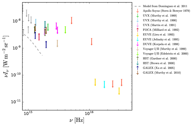
At the low end of the frequency range there have been several estimates of the CUB derived from galaxy counts using the Space Telescope Imaging Spectrograph (STIS) on HST (Gardner et al., 2000; Brown et al., 2000) and the GALaxy Evolution eXplorer satellite (GALEX, Xu et al., 2005), which we give as lower limits to the total CUB, since these estimates lack the diffuse contribution from inter-cluster gas. We also include an earlier estimate using a balloon-borne UV-imaging telescope centred at 200 nm (Milliard et al., 1992). For upper limits where Galactic emission must be subtracted, GALEX has also provided the most recent estimate of the CUB (Murthy et al., 2010). Prior to this, we include contributions from the following experiments: the Ultraviolet Spectrometer (UVS) aboard the Voyager spacecraft (Murthy et al., 1999; Edelstein et al., 2000); the Diffuse Ultraviolet Experiment (DUVE, Korpela et al., 1998); and a series of UV instruments flown aboard the Space Shuttle Columbia in 1986 (Murthy et al., 1989, 1990; Martin et al., 1991). At the high frequency end of the range (tens of nanometres), estimates have been taken from measurements made on the Apollo- Soyuz mission by the Extreme UltraViolet Telescope (EUVT, Stern & Bowyer, 1979), covering 9–59 nm. Lastly we report findings on the total diffuse UV background (so again, upper limits on the CUB) from the Extreme UltraViolet Explorer’s (EUVE) Deep Survey (DS) telescope at 10, 17 and 24 nm (Lieu et al., 1993; Jelinsky et al., 1995).
Figure 5 displays the current status on the CUB, showing a general decline in intensity from beginning to end, with no interesting features visible due to the lack of constraining data at these wavelengths.
3.6 The cosmic X-ray background (CXB)
[–Hz,
–30 nm]
As we move to even higher energies we arrive at the CXB, spanning the range from to Hz. It is now generally believed that the astrophysical processes producing the CXB are dominated by the accretion disks around AGN (e.g., Comastri et al., 1995), which are hot enough to emit thermal bremsstrahlung photons observed in the X-ray range. This source of radiation is negligible at lower frequencies, where we largely see thermal energy (leftover from the early Universe and from warm dust) and nuclear energy (released in the form of photons from nuclear reactions in the cores of stars); however, at X-ray and -ray frequencies gravitational energy is the dominant mechanism sourcing the spectrum through accretion of gas.
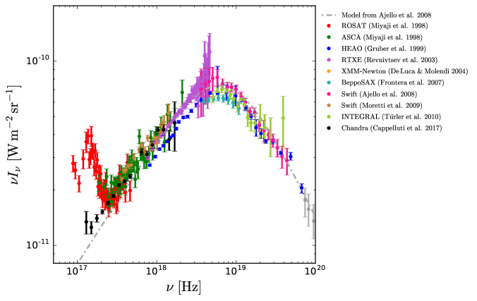
There have been lots of measurements of the CXB within the past couple of decades, and it contains yet another peak in the CB spectrum, with important astronomical and cosmological implications. Between 1 and 10 keV (electron-volts being the primary unit used by X-ray astronomers) we will use a joint data analysis from Miyaji et al. (1998) that combined observations form two Proportion Sensitive Proportional Counters (PSPC) on ROSAT and two Gas Imaging Spectrometers (GIS) on the Advanced Satellite for Cosmology and Astrophysics (ASCA), plus data from Swift’s X-Ray Telescope (XRT, Moretti et al., 2009), and XMM-Newton’s European Photon Imaging Camera (EPIC, De Luca & Molendi, 2004). There also exist CXB observations from Chandra’s Advanced CCD Imaging Spectrometer (ACIS), described by Hickox & Markevitch (2006) and later updated by Cappelluti et al. (2017); we use the latter work here (although they are largely consistent with each other). Next, between 3 and 20 keV, we include the Revnivtsev et al. (2003) CXB results obtained from the Rossi X-ray Timing Explorer (RXTE) using the Proportion Counter Array (PCA), and between 16 and 45 keV results from the BeppoSAX Phoswich Detection System (PDS, Frontera et al., 2007).
Moving into the hard X-ray portion of the spectrum, the CXB has been observed from 15 to 180 keV by the INTErnational Gamma-Ray Astrophysics Laboratory (INTEGRAL) via the Imager on-Board the INTEGRAL Satellite (IBIS, Türler et al., 2010), and another instrument of Swift’s, the Burst Array Telescope (BAT, Ajello et al., 2008). Lastly we have earlier measurements made across almost the entire CXB spectrum by a single telescope, namely the High Energy Astrophysics Observatory (HEAO), where Gruber et al. (1999) (and references therein) determine the CXB between 3 and 275 keV using a combination of HEAO’s Low Energy Detector (LED), Medium Energy Detector (MED) and High Energy Detector (HED).
Similar to the COB and CIB, there has been much interest in resolving the sources responsible for producing the CXB, using the high angular resolution offered by current-generation X-ray telescope. For instance, observations using XMM-Newton have been able to resolve into discrete sources nearly 100 of the low-energy end of the CXB, but the fraction drops to about 50 at the mid range (Worsley et al., 2005; Xue et al., 2012), and at high energies, observations with NuSTAR have only managed to resolve about 30 of the CXB (Harrison et al., 2016). While detecting the X-ray emitters that contribute to the CXB is astrophysically interesting, we have not included these measurements in our compilation, since the absolute value of the CXB is much more attainable in this frequency range than in the infrared to ultraviolet range (due to much less foreground contamination).
In Fig. 6 we have plotted all of the above data. A fourth maximum in the CB is seen to peak at about Hz (20 keV), with an energy density that is more than two orders of magnitude below that of the CIB and COB. There is broad consensus between each CXB evaluation; however, some of the measurements with small uncertainties do not appear to be in full agreement with the others, particularly at lower energies where foreground subtraction is more difficult. Presumably systematic errors (from calibration and foreground removal, for example), would reconcile these measurements; however, we have not made any attempt here to assess these effects, or to bring the measurements into better agreement. Nevertheless, it is clear that a simple thermal Bremsstrahlung spectrum broadly fits the data – this can be modelled as a double power law of the form
| (15) |
for specific parameters and . We have taken best-fit values for this model from Ajello et al. (2008) and plotted the resulting curve along with the data in Fig. 6.
3.7 The cosmic -ray
Background (CGB)
[Hz, nm]
The final portion of the CB is the CGB, which encompasses all frequencies greater than Hz. The primary contributors to the CGB are quasars/blazars (Inoue, 2014) and supernova explosions (Ruiz-Lapuente et al., 2001). Quasars and blazars emit jets of ultra-relativistic charged particles along the rotational axis of their accretion disks; photons can reach enormous energies by Compton scattering off these electrons, which we see if the jet is pointing close to our line of sight. Supernovae explosions, on the other hand, occur when a massive star exhausts its fuel at the end of its lifetime, resulting in a cataclysmic core collapse and the release of a huge amount of energy, including -rays. With about 100 supernovae occurring per year per redshift per square degree (Ruiz-Lapuente et al., 2001), their contribution to the CGB is believed to be small compared to that of quasars and blazars, but not negligible.
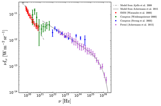
A high-energy cutoff occurs due to pair-production interactions between CGB photons and CIB photons (this is the same effect used to derive CIB upper limits, see de Jager & Harding, 1992). This cutoff is generally thought to be around 300 GeV, or Hz (Ajello et al., 2015), and gives a limit to the CGB – most higher energy photons are expected to have been converted into particles during their long intergalactic journey to the Earth.
For this highest energy part of the CB we incorporate data from the Gamma-Ray Spectrometer (GRS) aboard the Solar Maximum Mission (SMM) for energies between 0.3 and 2.7 MeV (Watanabe et al., 2000), and from the COMPton TELescope (COMPTEL) on the Compton Gamma-Ray Observatory between 1 MeV and 20 MeV (Weidenspointner et al., 2000). There have also been important measurements of the CGB from Compton’s Energetic Gamma-Ray Experiment Telescope (EGRET), which had an effective waveband of 30 MeV to 20 GeV (Strong et al., 2004). Compton’s successor was the Fermi Gamma-Ray Telescope, which was able to make major improvements in the high-energy spectrum between 0.1 and 500 GeV using its Large Array Telescope (LAT, Ackermann et al., 2015). Despite these improvements, we still use the COMPTEL and EGRET data, since they bridge the gap nicely between the 2.7 MeV SMM measurement and the 0.1 GeV Fermi measurement.
Figure 7 shows the CGB estimates obtained using the experiments mentioned above. The high-energy cutoff is clearly observed in the Fermi data, since the slope is seen to become steeper at around Hz (40 GeV). Although there is broad agreement on the shape, not all estimates are consistent within the uncertainties, again pointing to systematic effects between experiments. Given Fermi’s greater resolution and ability to resolve -ray point sources compared with Compton, it is expected to be able to isolate extragalactic sources more easily and so separate these out from the Galactic background signal. In Fig. 7 we indicate with a solid line a simple power-law model with an exponential cutoff (Ackermann et al., 2015), which approximately describes the data.
3.8 The complete cosmic background
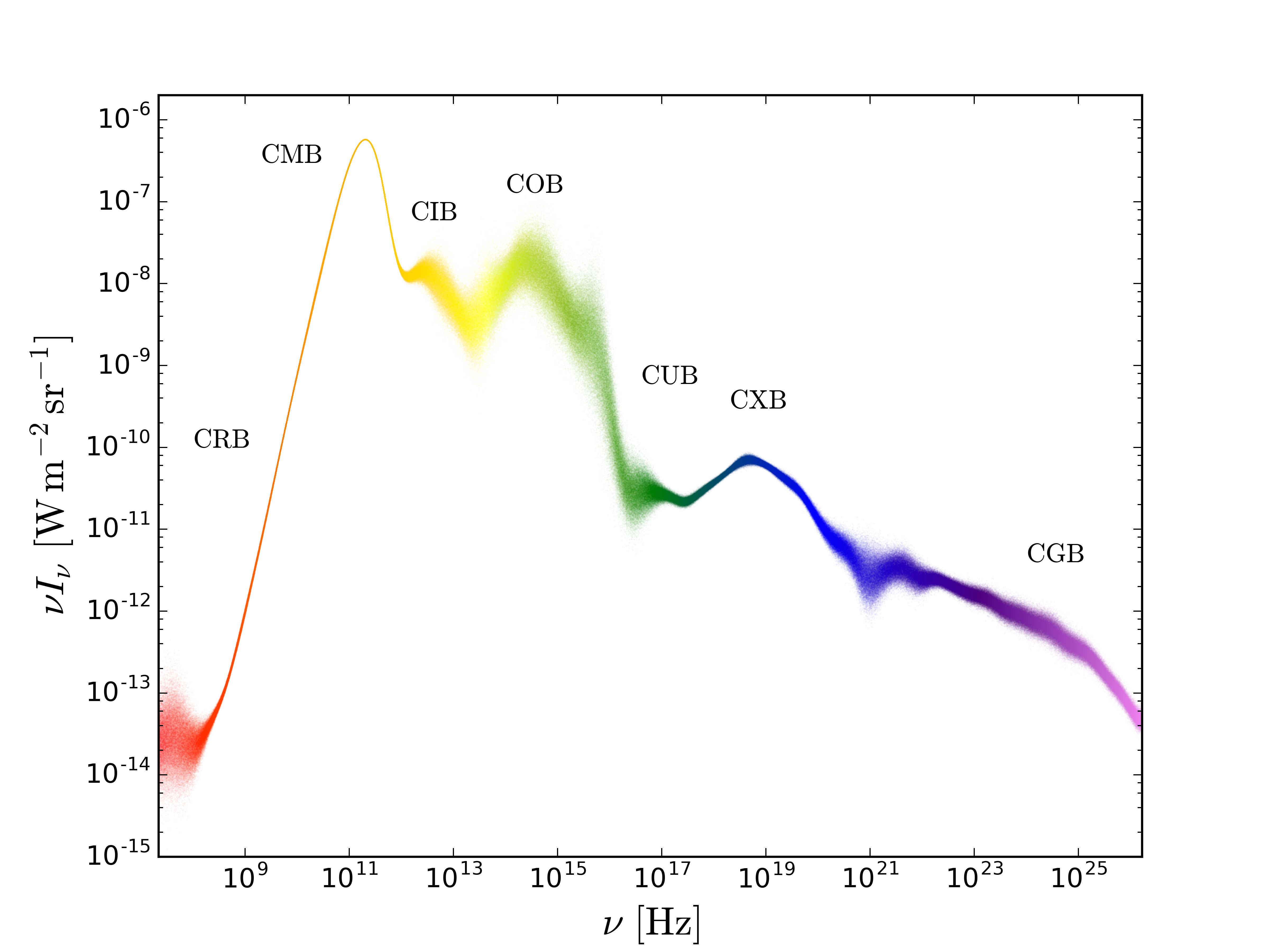
We can now piece together the cosmic background radiation over the entire electromagnetic spectrum. Combining Figs. 1 to 7 gives the overall result, shown in Fig. 8. This represents the energy distribution of photons permeating the Universe, and includes radiation emitted from sources over the whole of cosmic history.
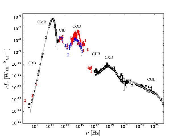
As an alternative way of presenting the data, we have produced a best-guess continuous curve from the discrete measurements of Fig. 8. The thickness of the line here is proportional to the uncertainties. These were estimated by extrapolating and smoothing a set of continuous curves along the upper and lower uncertainty values of each data point in Fig. 8 (if only an upper/lower limit is present, this is taken to be the upper/lower uncertainty value), and letting the width be , corresponding to upper and lower two-sided 95 confidence interval limits. This procedure was used to determine the spread between the two curves, which is shown as a “splatter plot” in Fig. 9. Where the curve is narrow, the spectrum is well constrained, but where the spread is wide there is still lots of room for improving the measurements.
4 Line emission perturbations
So far every emission process we have discussed has been spectrally continuous – synchrotron radiation, blackbody radiation, thermal bremsstrahlung radiation and Compton processes each depend smoothly on the energies of the particles involved. However, line emission (essentially Dirac delta functions in the cosmological rest frame) are also present in the CB. If we could extract these discrete features, this would provide information not only about physical conditions projected along the line of sight, but also about the distribution of redshifts (and therefore distances) of the sources of emission. The technique of detecting line emission at different frequencies over large solid angles is known as “intensity mapping” (e.g., Hogan & Rees, 1979; Scott & Rees, 1990; Madau et al., 1997; Suginohara et al., 1999; Chang et al., 2008; Mao et al., 2008; Kovetz et al., 2017), and can be viewed as a way to 3-dimensionally map volumes of space. The sensitivity required to successfully glean statistical information on cosmological scales from intensity mapping is quite modest, but the most challenging aspect of these experiments is the removal of foreground emission and systematic effects. Experimental results are only recently beginning to appear, as experiments are being developed to overcome these challenges. In this section we discuss the effects on the CB of a few of the most cosmologically important lines by estimating their monopole terms as functions of redshift, and hence their contribution to the spectrum of the monopole. We will also present some recent experimental attempts to constrain these line contributions to the background sky.
4.1 The Hi line
The spin-flip transition in neutral hydrogen, Hi, also known as the 21-cm line, has a rest-frame frequency of 1420 MHz, corresponding to 0.00587 eV. It comes from the transition between the aligned (triplet) and anti-aligned (singlet) electron-proton spin states, the latter of which has slightly lower energy. Although intrinsically weak (this is a forbidden transition, with a lifetime of around 10 million years), the fact that hydrogen is the most abundant element in the Universe makes this line an important tracer of neutral gas everywhere, including for cosmological large-scale structure. There is currently much promise for the 21-cm line to probe the epoch of reionization (EoR) at , which marks the end of the cosmic “dark ages”, where we currently only have indirect information (see Furlanetto et al., 2006, for a review of the prospects for 21-cm intensity mapping).
Prior to the EoR, the intensity of the 21-cm mean background depends largely on the hydrogen spin temperature, , a measure of the ratio of atoms in the singlet versus triplet configurations:
| (16) |
Here K is the transition energy in temperature units. Also necessary for calculating the line intensity is the mean fraction of neutral hydrogen, , since only bound hydrogen atoms emit 21-cm radiation. The evolution of the neutral fraction is particularly important following the EoR, when hydrogen transitioned from being mostly neutral to its present state of being mostly ionized. Expressing the intensity as a CMB-subtracted brightness temperature (which can be converted to SI units through Eq. 5), we have (Furlanetto, 2006)
| (17) |
where , and the factor of 27 arises from cosmological parameters within the best-fit CDM model, combined with the properties of the line.
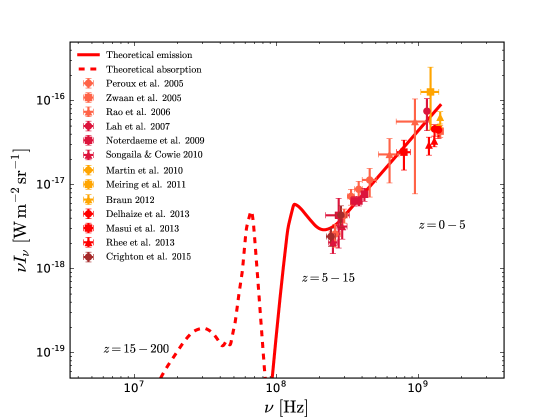
Models of the evolution of the gas density and temperature, including ionization sources in the early Universe, can be used to calculate the spin temperature and ionization fraction as a function of redshift (e.g., Pritchard & Loeb, 2008; Mirocha et al., 2013; Davé et al., 2013; Rahmati et al., 2013; Barnes & Haehnelt, 2014; Bird et al., 2014; Yajima & Khochfar, 2015; Ghara et al., 2015; Padmanabhan et al., 2017). Here we have taken the results of several representative studies (Furlanetto, 2006; Pritchard & Loeb, 2008; Mirocha et al., 2013; Yajima & Khochfar, 2015; Ghara et al., 2015) between and and produced an average spectrum, shown in Fig. 10; this gives merely a rough estimate of the integrated 21-cm line intensity, and hence we have not displayed any uncertainty. At low frequencies (coming from epochs above ), the 21-cm line is seen in absorption against the CMB, instead of emission, because the hydrogen gas adiabatically cools below the CMB temperature. We have plotted the absolute value of this negative temperature difference as the dashed line in Fig. 10.
We now turn our attention to observations. The background 21-cm brightness temperature is difficult to measure directly, since it is hard to absolutely calibrate most radio detectors, and there are also continuum foregrounds that will contaminate the measurements. However, the 21-cm monopole can be determined indirectly by estimating , the neutral hydrogen density in units of the cosmological critical density, performed via a census of hydrogen absorption (or emission) lines. In the limit where (applicable when ) Eq. (17) can be simplified and estimated in terms of . Another approach is to cross-correlate noisy radio maps of 21-cm emission with 3D maps of galaxies. This measures the extent to which clusters with galaxies, rather than measuring the or the 21-cm monopole directly. When can then use our understanding of structure formation to infer the hydrogen abundance.
Such measurements of have been carried out using radio surveys (Zwaan et al., 2005; Lah et al., 2007; Martin et al., 2010; Braun, 2012; Rhee et al., 2013; Delhaize et al., 2013; Masui et al., 2013) and optical surveys (Péroux et al., 2005; Rao et al., 2006; Noterdaeme et al., 2009; Songaila & Cowie, 2010; Meiring et al., 2011; Crighton et al., 2015). Over the redshift range of –5, has been found to be of the order 100 K (roughly – at these frequencies). We show these estimates in Fig. 10, along with the theoretical calculations discussed above. Future experiments promise to probe the “step” expected at around 100 MHz, whose detailed profile will tell us about the processes that reionized the Universe.
4.2 Lines from early Universe chemistry
In the standard picture of structure formation, there are no important atomic processes happening between the time of cosmological recombination at a redshift of about 1000 (when the Universe was a few hundred thousand years old) and when the first objects collapsed and turned into stars at redshifts perhaps around 15 (when the Universe was a few hundred million years old). The formation of the first stars began the process of creation of the heavy elements that make the world so interesting today. However, chemical processes started before that, operating on the hydrogen, helium and trace amounts of lithium and other light elements that were produced primordially (see e.g., Galli & Palla, 2013). Molecular hydrogen was able to form via intermediary species such as H, H-, and HeH+, and was a major coolant for the formation of the first structures. Detection of lines from this early H2-cooling phase would be an important probe of the early Universe, but will be extremely challenging (although there is hope through future space missions, such as the Origins Space Telescope, Meixner et al., 2016).
Additionally there will be trace amounts of other molecules, such as HD and LiH, and there have been suggestions that these may be important at certain epochs. Despite lithium having very low abundance in the early Universe, at one point it was proposed (Loeb, 2001; Stancil et al., 2002) that absorption of the CB by the (redshifted) line of neutral Li might be important. However, it was shown (Switzer & Hirata, 2005) that the small excess of UV photons created during hydrogen recombination is enough to keep lithium ionized during these dark ages, and hence the line is cosmologically unimportant. In a similar way, the possibility of free-free absorption by H- in the early Universe (Black, 2006) was substantially revised down to negligible levels (Schleicher et al., 2008). There may still be scope for early Universe chemistry to have observational consequences in the distant future, but in the meantime attention on line processes is focused on the more accessible lower redshift regime.
4.3 The Cii line
There are observable IR fine-structure lines emitted from elements such as carbon, nitrogen and oxygen that are important for cooling in star-forming regions of galaxies. Modelling these line emission processes is more complicated than for Hi, with many possible spin transitions from not only neutral atoms but ionized atoms as well, and with radiative transfer effects needing to be included to account for the diverse physical conditions. Nevertheless the general approach to estimating the background contribution remains more or less the same. As a specific example, we will first focus on emission from Cii, singly ionized carbon.
Since carbon is produced in stars and the – transition temperature (91 K) matches that of photo-dissociation regions near to bright stars, Cii plays an important role in cooling (Dalgarno & McCray, 1972). In fact it can be the brightest line in galaxy spectra, containing up to 0.1 of the bolometric luminosity (Crawford et al., 1985). This fine-structure line is at 157.7 m (or 1900 MHz), placing it in the far-IR.
Two approaches have been developed for modelling this transition in the cosmological context. The first follows directly from the discussion of Hi, calculating the spin temperature as a function of redshift through Eq. (17) (Gong et al., 2012; Kusakabe & Kawasaki, 2012). The second method, outlined in Visbal & Loeb (2010), Uzgil et al. (2014) and Silva et al. (2015), is simpler, and uses an integral over emissive sources assuming no absorption along the line of sight, using the following equation:
| (18) |
Here the line element contains the cosmology, and is the proper volume emissivity of Cii radiation at rest frequency . If all Cii emission comes from gas in galaxies located in dark matter halos, we can write the proper volume emissivity as
| (19) |
where is the dark matter halo mass function (e.g., Tinker et al., 2008), is the minimum halo mass required to form a galaxy and is the Cii luminosity at frequency for a dark matter halo of mass . We then make the further simplification that the Cii luminosity of a galaxy is proportional to the star-formation rate,
| (20) |
where the constant can be calibrated through observations of nearby galaxies and has the typical value (in solar units) of (Righi et al., 2008), and is the star-formation rate. The delta function here ensures that the line emission occurs at the proper frequency.
For , we can write
| (21) |
where and are the baryonic and matter density fractions of the Universe and is the fraction of baryons contained in stars, which form on a typical timescale . Integrating the volume emissivity over redshift then yields
| (22) |
From this equation it can be seen that one generally has to estimate and , which could in principle depend on the mass and lead to more complicated models. Improvements can also be considered, including treating heavy element abundance (Yue et al., 2015), and having depend on galaxy type, but these do not change the order of magnitude of the result.
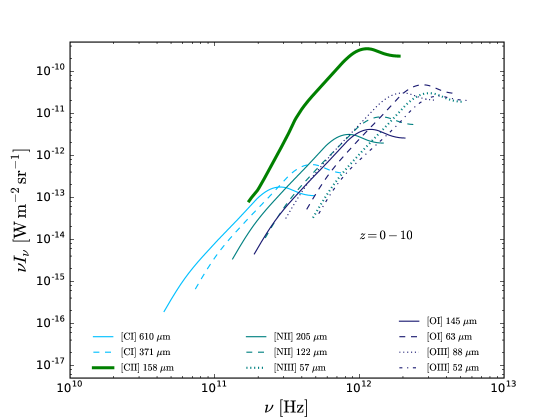
4.4 Other fine-structure lines
Other far-IR lines from low-ionization states of common elements are also prominent in galaxy spectra. To gauge the contribution to the CB from other major cooling lines, we can use Eq. (22) to scale the cosmic Cii monopole spectrum, since it just depends on and for each line. Righi et al. (2008) provides ratios for two Ci transitions (610 and 371 m), two Oi transitions (145 and 63 m), two Oiii transitions (88 and 52 m), two Nii transitions (122 and 205 m) and one Niii transition (57 m). We plot these line intensities alongside that of Cii in Fig. 11. Other studies have approached the calculation in different ways (e.g., Kusakabe & Kawasaki, 2012), but give generally similar results.
4.5 CO lines
The most abundant molecule in the Universe is , but due to the lack of dipole transitions it is hard to detect. The predominant tracer of molecular gas in galaxies is then carbon monoxide (see Bolatto et al., 2013, for a review of carbon monoxide and in star-forming galaxies). The main lines are rotational-vibrational transitions from the total angular momentum state to , and the photons emitted occur in the millimetre and submillimetre bands at multiples of 115 GHz.
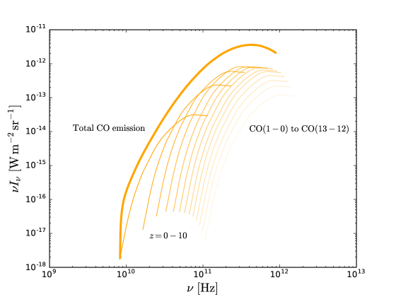
Several studies have estimated the global CO emission using a similar approach to Section 4.3, by scaling the IR galaxy luminosity (Lidz et al., 2011; Carilli, 2011; Pullen et al., 2013; Li et al., 2016) or the star-formation rate (Breysse et al., 2014). Alternatively, one can use a line luminosity to star-formation rate ratio, but model the star-formation rate through the dark matter halo abundance (Righi et al., 2008; Padmanabhan, 2018), or use the output of large-scale galaxy formation simulations (Gong et al., 2011). There is general agreement that the expected signal is in the K regime, although predictions vary in detail. We have taken an average of the above models and calculated the intensity out to , which we show in Fig. 12.
This estimate can be extended out to the higher CO transitions by scaling to different values of (from e.g., Righi et al., 2008; Visbal & Loeb, 2010) and scaling the rest frequency of each line. We include these curves in Fig. 12 up to , along with the sum of all CO transition intensities.
4.6 The Ly line
As well as radio and far-IR lines, the spectra of galaxies also have prominent emission lines at visible wavelengths. Of particular interest is the Lyman line at nm (or Hz), which results from a transition from the to state in hydrogen. This line plays an important role in the opacity of the ISM because of the abundance of hydrogen and the supply of ultraviolet continuum photons from hot young stars.
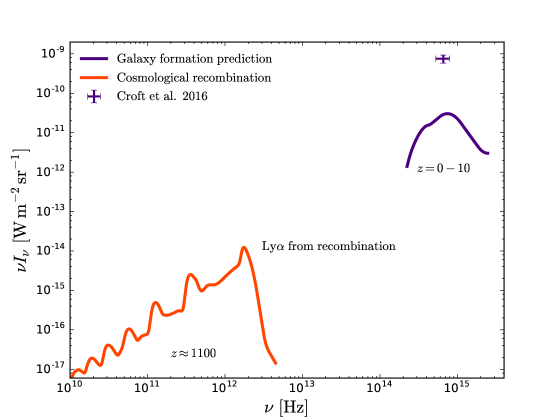
Theoretical intensity models have been constructed (e.g., Pullen et al., 2013; Silva et al., 2013; Gong et al., 2014), taking into account radiative and collisional recombinations, with stars being the sources of radiation. In contrast to CO and Cii, which are generally confined to the inner parts of galaxies, hydrogen emission also comes from diffuse gas in galaxy halos and to some extent from the intergalactic medium. Detailed calculations involve modelling radiative transfer in clumpy and dusty regions, with a great deal of uncertainty in the specifics. We merely display an average of representative results in Fig. 13 for redshifts up to .
Ly emission can also be estimated empirically. For example Croft et al. (2016) recently measured the brightness fluctuations of the Ly emission by cross-correlating optical spectra with galaxies tracing the large-scale structure of the Universe. This measures the product of the mean Ly intensity and linear bias factor (parameterizing the cosmic large-scale clumpiness of emission), and it was found that at , assuming . We have included this measurement in Fig. 13. Although the overall bias is uncertain, for any reasonable value this result is roughly an order of magnitude larger than the theoretical estimates. The extra emission could come from an unresolved population of Ly emitters, which have not been taken into account in the models, or could be due to a number of possible systematic errors. In summary, in this redshift range the total Ly brightness is highly uncertain, both in terms of theoretical models and empirically. Decreasing this uncertainty is currently an area of active research in the community studying galaxy evolution.
Another cosmologically relevant perturbation to the CB spectrum resulting from hydrogen (and, to a lesser extent, helium) is from the high redshift recombination (or “combination”, since the atoms had never previously been neutral) process, occurring at redshift . Numerical calculations have shown that this produces a distortion to the CMB of amplitude (Dubrovich & Shakhvorostova, 2004; Kholupenko et al., 2005; Wong et al., 2006; Chluba et al., 2007). Recombination contributes photons not only from the Ly transition, but from all possible hydrogen and helium transitions, including 2-photon processes. We show in Fig. 13 the specific results from Chluba et al. (2007), and note that the Ly transition discussed above corresponds to the highest peak, while the remaining peaks come from other hydrogen transitions. The detection of these spectral deviations will be extremely challenging, but there are attempts being discussed, for instance by a future mission like PIXIE (Kogut et al., 2011).
4.7 The Fe X-ray line
The last line we will consider is the 6.4-keV X-ray line from iron atoms, sometimes called the K line. This is seen in AGN accretion disk spectra, being the brightest and most prominent spectral feature (e.g., Nandra et al., 1989; Pounds et al., 1989; Fukazawa et al., 2011). In this process, iron atoms become ionized by losing an inner shell electron, and the gap is subsequently filled by an outer electron, emitting a 6.4 keV, or Hz, photon. Intensity mapping of this particular line has been suggested as a tool for investigating galaxy evolution by probing the power spectrum of highly redshifted AGN in a large-area survey (Hütsi et al., 2012; Kolodzig et al., 2013).
Continuing with our simple modelling approach, we can estimate the contribution to the sky brightness of the Fe line. Note that this should be considered as an upper limit, since in practice not every dark matter halo will host an AGN (Akylas et al., 2012; Ueda et al., 2014). To do this, we again want to scale Eq. (22). X-ray iron line luminosity measurements from AGN (Ricci et al., 2014) can be used to estimate to be about W, and combining this with typical AGN star-formation rates of around M⊙ yr-1 (Mullaney et al., 2015) yields . The resulting scaled spectrum is plotted in Fig. 14, with downward arrows suggesting that it should be considered as an upper limit only.
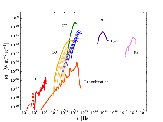
4.8 Complete line background
Figure 14 combines each line spectrum presented in this section. These are of course not the only line emission processes occurring in the Universe, but can be considered to be the most luminous or the most abundant. In comparison with the complete CB, these line emission features lie far below the continuum background, and it would be very hard to detect any of these features in the CB monopole. Despite this, there is a real prospect of being able to see the spatially fluctuating part of some of these brighter lines through future intensity mapping experiments.
5 Beyond the monopole
We have focused here on the average sky brightness at each frequency, i.e., the spectrum of the cosmic monopole. This is proportional to the energy density as a function of frequency, and hence provides important information on the census of energy processes that occur through the history of our Universe. An obvious next step would be to characterize the spectrum of the cosmic dipole. In practice this is dominated by the fact that we are moving relative to a frame defined by radiation on very large scales. Variations in the dipole caused by there being more structure on one side of the sky than another are subdominant to this relative-frame “boosting” effect, hence the spectrum of the cosmic dipole is essentially the same as the monopole (just lower by a factor of about because for our motion, Scott & Smoot, 2016; Burigana et al., 2017). Hence measurement of the spectrum of the dipole pattern is not likely to provide much new information about the Universe. However, the same is not true about sky variations on smaller angular scales.
Considering the sky as purely a source of information about the Cosmos, one could encode this by determining the spectrum in every direction, or equivalently by measuring the spectrum for every spherical harmonic coefficient of sky emission (Scott et al., 2016). In the Universe (unlike for the Solar System or the Milky Way, or the typical experimental laboratory for that matter) there are no special directions – the Universe appears to be isotropic, at least in a statistical sense. This means that there are no special s for each multipole (as there would be in axial symmetry, where , for example). An additionally important fact is that on sufficiently large scales cosmological structure is of low contrast and hence evolves under linear perturbation theory, which means that there are no strong phase correlations and the 2-point correlation function contains the majority of the cosmological information. In harmonic space we can therefore restrict ourselves to determining the squares of the amplitudes of the spherical harmonic coefficients summed over for each multipole :
| (23) |
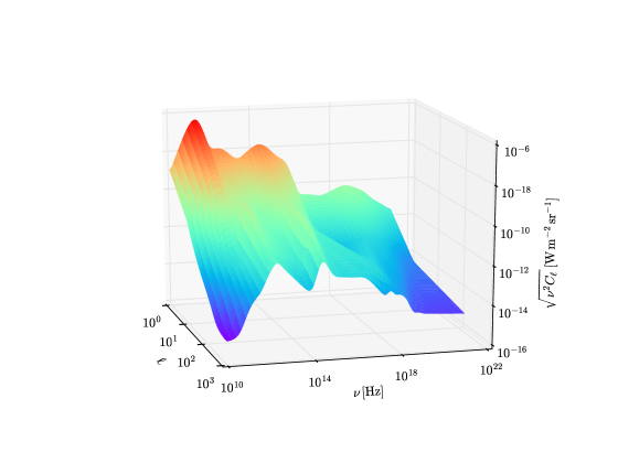
It is therefore possible to encompass most of the useful sky information by characterizing the frequency spectrum of this fluctuation power spectrum, or . We show a schematic representation of what these might look like in Fig. 15. In a sense this “power spectrum spectrum” is the blueprint describing just what sort of Universe we live in, and all the physical processes operating to give it its large-scale statistical properties.
Estimating these higher moments is much more challenging than determining the mean intensity of the sky, owing to the fact that not only must atmospheric, zodiacal and Galactic contributions be subtracted, but noise and systematic effects in experimental data must be fully understood and removed as well. In general the systematic effects are hard to control over a wide range of angular scales. The main exception comes from the CMB, by far the brightest component of the CB, whose multipole spectrum has been measured to high precision by the Planck satellite mission (Planck Collaboration XV, 2014). Further CB multipole moments have been estimated in the IR (Lagache et al., 2007; Matsuura et al., 2011; Hajian et al., 2012; Viero et al., 2013; Planck Collaboration XXX, 2014) and the optical (Kashlinsky et al., 2002; Thompson et al., 2007; Cooray et al., 2012; Zemcov et al., 2014; Mitchell-Wynne et al., 2015; Seo et al., 2015), as well as at higher X-ray and -ray energies (Śliwa et al., 2001; Cappelluti et al., 2013; Broderick et al., 2014). However, these are typically over only a restricted range of scales and there remains much more work to be done in order to extract all of the cosmological information from the background sky.
6 Conclusions
In this paper we have summarized recent measurements of the cosmic background radiation, in order to obtain a comprehensive perspective on the extragalactic photons that fill our sky. Spanning 18 orders of magnitude in frequency or wavelength, the CB requires a wide range of instruments and detector technologies to measure, and an understanding of many different astrophysical processes to interpret.
Photons are not the only particles that come to us from the distant Universe – there are also cosmic rays, neutrinos and gravitons. These can tell us about special places within galaxies (typically neutron stars, black holes, and galactic nuclei) from where they are emitted. In future such non-photon backgrounds might also provide more general information about cosmology and structure formation. But for now our view of the Cosmos is dominated by what we learn from the electromagnetic radiation background, which has been the subject of our review.
We split the CB into seven components, from radio to -rays, which we call the CRB, CMB, CIB, COB, CUB, CXB and CGB. Very broadly, the extragalactic radio emission comes from synchrotron radiation and the low-energy tail of the CMB, while the CMB is the redshifted thermal remnant of the hot early Universe. The CIB comes mainly from dust that has been heated by stars and re-radiated at cooler temperatures, while the COB comes from the stars directly. In the CUB we have a combination of scattered starlight and hot diffuse gas, while the CXB comes predominantly from the accretion disks of galactic nuclei. Lastly, CGB photons are primarily emitted from the ultra high-energy jets of galactic nuclei. In order to determine the cosmic average sky brightness, it is necessary to subtract the emission from the instrument, the Earth’s atmosphere, the Solar System and the Milky Way. This is challenging in most wavebands, and hence our knowledge of the CB is still quite incomplete.
Small amplitude spectral features should be present in the monopole spectrum, arising from line emission processes, and we have presented order-of-magnitude estimates for some of the most astrophysically important lines. The study of such line features is still in its infancy, but future experiments hold great promise through measurement of structure in 3D data cubes (“intensity mapping”) and of spatial correlations with other emission processes in the fluctuating sky.
The majority of statistical information present in the CB is encoded in higher-order multipole moments. Precise estimates of the power in these multipoles of the CMB pin down models of the early Universe, while at other wavebands we have cruder estimates of the correlated sky that tells us about the formation of structure at more recent epochs. One could imagine essentially having a full spectrum of the power at every angular scale on the sky. This “spectrum of the power spectrum” would encode a large fraction of the information accessible to us that characterizes our entire observable Universe.
Acknowledgements
This research was supported by the Natural Sciences and Engineering Research Council (NSERC) of Canada.
References
- Ackermann et al. (2015) Ackermann M., et al., 2015, Astrophys. J., 799, 86
- Ajello et al. (2008) Ajello M., et al., 2008, Astrophys. J., 689, 666
- Ajello et al. (2015) Ajello M., et al., 2015, Astrophys. J., 800, L27
- Akylas et al. (2012) Akylas A., Georgakakis A., Georgantopoulos I., Brightman M., Nandra K., 2012, Astron. Astrophys., 546, A98
- Altieri et al. (1999) Altieri B., et al., 1999, Astron. Astrophys., 343, L65
- Aravena et al. (2016) Aravena M., et al., 2016, Astrophys. J., 833, 68
- Arendt & Dwek (2003) Arendt R. G., Dwek E., 2003, Astrophys. J., 585, 305
- Ashby et al. (2013) Ashby M. L. N., et al., 2013, Astrophys. J., 769, 80
- Baldry et al. (2002) Baldry I. K., et al., 2002, Astrophys. J., 569, 582
- Barnes & Haehnelt (2014) Barnes L. A., Haehnelt M. G., 2014, Mon. Not. R. Astron. Soc., 440, 2313
- Bernstein (2007) Bernstein R. A., 2007, Astrophys. J., 666, 663
- Berta et al. (2011) Berta S., et al., 2011, Astron. Astrophys., 532, A49
- Béthermin et al. (2010) Béthermin M., Dole H., Beelen A., Aussel H., 2010, Astron. Astrophys., 512, A78
- Béthermin et al. (2012) Béthermin M., et al., 2012, Astron. Astrophys., 542, A58
- Bird et al. (2014) Bird S., Vogelsberger M., Haehnelt M., Sijacki D., Genel S., Torrey P., Springel V., Hernquist L., 2014, Mon. Not. R. Astron. Soc., 445, 2313
- Biteau & Williams (2015) Biteau J., Williams D. A., 2015, Astrophys. J., 812, 60
- Black (2006) Black J. H., 2006, Faraday Disc., 133, 27
- Bolatto et al. (2013) Bolatto A. D., Wolfire M., Leroy A. K., 2013, Annual Reviews Astron. Astrophys., 51, 207
- Boldt (1987) Boldt E., 1987, Phys. Rep., 146, 215
- Bond et al. (1986) Bond J. R., Carr B. J., Hogan C. J., 1986, Astrophys. J., 306, 428
- Bowyer (2001) Bowyer S., 2001, in Harwit M., ed., Symp. – Int. Astron. Union. Vol. 204, The Extragalactic Infrared Background and its Cosmological Implications. p. 123
- Bowyer et al. (2000) Bowyer S., Drake J. J., Vennes S., 2000, Annual Reviews Astron. Astrophys., 38, 231
- Braun (2012) Braun R., 2012, Astrophys. J., 749, 87
- Breysse et al. (2014) Breysse P. C., Kovetz E. D., Kamionkowski M., 2014, Mon. Not. R. Astron. Soc., 443, 3506
- Bridle (1967) Bridle A. H., 1967, Mon. Not. R. Astron. Soc., 136, 219
- Broderick et al. (2014) Broderick A. E., Pfrommer C., Puchwein E., Chang P., Smith K. M., 2014, Astrophys. J., 796, 12
- Brown et al. (2000) Brown T. M., Kimble R. A., Ferguson H. C., Gardner J. P., Collins N. R., Hill R. S., 2000, Astron. J., 120, 1153
- Burigana et al. (2017) Burigana C., et al., 2017, preprint, (arXiv:1704.05764)
- Cappelluti et al. (2013) Cappelluti N., et al., 2013, Astophys. J., 769, 68
- Cappelluti et al. (2017) Cappelluti N., et al., 2017, Astrophys. J., 837, 19
- Carilli (2011) Carilli C. L., 2011, Astrophys. J., 730, L30
- Carniani et al. (2015) Carniani S., et al., 2015, Astron. Astrophys., 584, A78
- Chabert & Braithwaite (2011) Chabert P., Braithwaite N., 2011, Physics of Radio-Frequency Plasmas. Cambridge University Press
- Chang et al. (2008) Chang T.-C., Pen U.-L., Peterson J. B., McDonald P., 2008, Phys. Rev. Lett., 100, 091303
- Chen et al. (2013) Chen C.-C., Cowie L. L., Barger A. J., Casey C. M., Lee N., Sanders D. B., Wang W.-H., Williams J. P., 2013, Astrophys. J., 776, 131
- Chluba et al. (2007) Chluba J., Rubiño-Martín J. A., Sunyaev R. A., 2007, Mon. Not. R. Astron. Soc., 374, 1310
- Clements et al. (1999) Clements D. L., Desert F.-X., Franceschini A., Reach W. T., Baker A. C., Davies J. K., Cesarsky C., 1999, Astron. Astrophys., 346, 383
- Comastri et al. (1995) Comastri A., Setti G., Zamorani G., Hasinger G., 1995, Astron. Astrophys., 296, 1
- Condon et al. (2012) Condon J. J., et al., 2012, Astrophys. J., 758, 23
- Cooray (2016) Cooray A., 2016, R. Soc. Open Sci., 3, 150555
- Cooray et al. (2012) Cooray A., et al., 2012, Nature, 490, 514
- Crawford et al. (1985) Crawford M. K., Genzel R., Townes C. H., Watson D. M., 1985, Astrophys. J., 291, 755
- Crighton et al. (2015) Crighton N. H. M., et al., 2015, Mon. Not. R. Astron. Soc., 452, 217
- Croft et al. (2016) Croft R. A. C., et al., 2016, Mon. Not. R. Astron. Soc., 457, 3541
- Dalgarno & McCray (1972) Dalgarno A., McCray R. A., 1972, Annual Reviews Astron. Astrophys., 10, 375
- Davé et al. (2013) Davé R., Katz N., Oppenheimer B. D., Kollmeier J. A., Weinberg D. H., 2013, Mon. Not. R. Astron. Soc., 434, 2645
- De Luca & Molendi (2004) De Luca A., Molendi S., 2004, Astron. Astrophys., 419, 837
- Delhaize et al. (2013) Delhaize J., Meyer M. J., Staveley-Smith L., Boyle B. J., 2013, Mon. Not. R. Astron. Soc., 433, 1398
- Dicke et al. (1965) Dicke R. H., Peebles P. J. E., Roll P. G., Wilkinson D. T., 1965, Astrophys. J., 142, 414
- Domínguez et al. (2011) Domínguez A., et al., 2011, Mon. Not. R. Astron. Soc., 410, 2556
- Driver et al. (2016) Driver S. P., et al., 2016, Astrophys. J., 827, 108
- Dubrovich & Shakhvorostova (2004) Dubrovich V. K., Shakhvorostova N. N., 2004, Astron. Lett., 30, 509
- Dwek & Krennrich (2013) Dwek E., Krennrich F., 2013, Astropart. Phys., 43, 112
- Edelstein et al. (2000) Edelstein J., Bowyer S., Lampton M., 2000, Astrophys. J., 539, 187
- Fabian & Barcons (1992) Fabian A. C., Barcons X., 1992, Annual Reviews Astron. Astrophys., 30, 429
- Fazio et al. (2004) Fazio G. G., et al., 2004, Astrophys. J., Suppl. Ser., 154, 39
- Finkbeiner et al. (2000) Finkbeiner D. P., Davis M., Schlegel D. J., 2000, Astrophys. J., 544, 81
- Finke et al. (2010) Finke J. D., Razzaque S., Dermer C. D., 2010, Astrophys. J., 712, 238
- Fixsen (2009) Fixsen D. J., 2009, Astrophys. J., 707, 916
- Fixsen et al. (1996) Fixsen D. J., Cheng E. S., Gales J. M., Mather J. C., Shafer R. A., Wright E. L., 1996, Astrophys. J., 473, 576
- Fixsen et al. (2004) Fixsen D. J., Kogut A., Levin S., Limon M., Lubin P., Mirel P., Seiffert M., Wollack E., 2004, Astrophys. J., 612, 86
- Fixsen et al. (2011) Fixsen D. J., et al., 2011, Astrophys. J., 734, 5
- Franceschini & Rodighiero (2017) Franceschini A., Rodighiero G., 2017, Astron. Astrophys., 603, A34
- Franceschini et al. (2008) Franceschini A., Rodighiero G., Vaccari M., 2008, Astron. Astrophy., 487, 837
- Frontera et al. (2007) Frontera F., et al., 2007, Astrophys. J., 666, 86
- Fujimoto et al. (2016) Fujimoto S., Ouchi M., Ono Y., Shibuya T., Ishigaki M., Nagai H., Momose R., 2016, Astrophys. J. Suppl. Ser., 222, 1
- Fukazawa et al. (2011) Fukazawa Y., et al., 2011, Astrophys. J., 727, 19
- Furlanetto (2006) Furlanetto S. R., 2006, Mon. Not. R. Astron. Soc., 371, 867
- Furlanetto et al. (2006) Furlanetto S. R., Oh S. P., Briggs F. H., 2006, Phys. Rep., 433, 181
- Galli & Palla (2013) Galli D., Palla F., 2013, Ann. Rev. Astron. Astrophys., 51, 163
- Gardner et al. (2000) Gardner J. P., Brown T. M., Ferguson H. C., 2000, Astrophys. J., 542, L79
- Gervasi et al. (2008) Gervasi M., Tartari A., Zannoni M., Boella G., Sironi G., 2008, Astrophys. J., 682, 223
- Ghara et al. (2015) Ghara R., Choudhury T. R., Datta K. K., 2015, Mon. Not. R. Astron. Soc., 447, 1806
- Giacconi et al. (1962) Giacconi R., Gursky H., Paolini F. R., Rossi B. B., 1962, Phys. Rev. Lett., 9, 439
- Gilli et al. (2007) Gilli R., Comastri A., Hasinger G., 2007, Astron. Astrophys., 463, 79
- Gilmore et al. (2012) Gilmore R. C., Somerville R. S., Primack J. R., Domínguez A., 2012, MNRAS, 422, 3189
- Gong et al. (2011) Gong Y., Cooray A., Silva M. B., Santos M. G., Lubin P., 2011, Astrophys. J., 728, L46
- Gong et al. (2012) Gong Y., Cooray A., Silva M., Santos M. G., Bock J., Bradford C. M., Zemcov M., 2012, Astrophys. J., 745, 49
- Gong et al. (2014) Gong Y., Silva M., Cooray A., Santos M. G., 2014, Astrophys. J., 785, 72
- Gruber et al. (1999) Gruber D. E., Matteson J. L., Peterson L. E., Jung G. V., 1999, Astrophys. J., 520, 124
- Gush et al. (1990) Gush H. P., Halpern M., Wishnow E. H., 1990, Phys. Rev. Lett., 65, 537
- Hajian et al. (2012) Hajian A., et al., 2012, Astrophys. J., 744, 40
- Halpern et al. (1988) Halpern M., Benford R., Meyer S., Muehlner D., Weiss R., 1988, Astrophys. J., 332, 596
- Harrison et al. (2016) Harrison F. A., et al., 2016, Astrophys. J., 831, 185
- Hasinger (1996) Hasinger G., 1996, Astron. Astrophys. Suppl. Ser., 120, C607
- Hauser & Dwek (2001) Hauser M. G., Dwek E., 2001, Annual Reviews Astron. Astrophys., 39, 249
- Henry et al. (2015) Henry R. C., Murthy J., Overduin J., Tyler J., 2015, Astrophys. J., 798, 14
- Hickox & Markevitch (2006) Hickox R. C., Markevitch M., 2006, Astrophys. J., 645, 95
- Hogan & Rees (1979) Hogan C. J., Rees M. J., 1979, Mon. Not. R. Astron. Soc., 188, 791
- Hopwood et al. (2010) Hopwood R., et al., 2010, Astrophys. J., 716, L45
- Hütsi et al. (2012) Hütsi G., Gilfanov M., Sunyaev R., 2012, Astron. Astrophys., 547, A21
- Inoue (2014) Inoue Y., 2014, preprint, (arXiv:1412.3886)
- Inoue et al. (2013) Inoue Y., Inoue S., Kobayashi M. A. R., Makiya R., Niino Y., Totani T., 2013, Astrophys. J., 768, 197
- Jelinsky et al. (1995) Jelinsky P., Vallerga J. V., Edelstein J., 1995, Astrophys. J., 442, 653
- Kashlinsky et al. (2002) Kashlinsky A., Odenwald S., Mather J., Skrutskie M. F., Cutri R. M., 2002, Astrophys. J., 579, L53
- Kawara et al. (2017) Kawara K., Matsuoka Y., Sano K., Brandt T. D., Sameshima H., Tsumura K., Oyabu S., Ienaka N., 2017, Publ. Astron. Soc. Jpn., 69, 31
- Keenan et al. (2010) Keenan R. C., Barger A. J., Cowie L. L., Wang W.-H., 2010, Astrophys. J., 723, 40
- Khaire & Srianand (2018) Khaire V., Srianand R., 2018, preprint, (arXiv:1801.09693)
- Kholupenko et al. (2005) Kholupenko E. E., Ivanchik A. V., Varshalovich D. A., 2005, Gravit. Cosmology, 11, 161
- Kogut et al. (2011) Kogut A., et al., 2011, J. Cosmology Astropart. Phys., 7, 025
- Kolodzig et al. (2013) Kolodzig A., Gilfanov M., Hütsi G., Sunyaev R., 2013, Astron. Astrophys., 558, A90
- Korpela et al. (1998) Korpela E. J., Bowyer S., Edelstein J., 1998, Astrophys. J., 495, 317
- Kovetz et al. (2017) Kovetz E. D., et al., 2017, preprint, (arXiv:1709.09066)
- Kusakabe & Kawasaki (2012) Kusakabe M., Kawasaki M., 2012, Mon. Not. R. Astron. Soc., 419, 873
- Lacki (2010) Lacki B. C., 2010, Mon. Not. R. Astron. Soc., 406, 863
- Lagache et al. (2005) Lagache G., Puget J.-L., Dole H., 2005, Annual Reviews Astron. Astrophys., 43, 727
- Lagache et al. (2007) Lagache G., Bavouzet N., Fernandez-Conde N., Ponthieu N., Rodet T., Dole H., Miville-Deschênes M.-A., Puget J.-L., 2007, Astrophys. J., 665, L89
- Lah et al. (2007) Lah P., et al., 2007, Mon. Not. R. Astron. Soc., 376, 1357
- Levin et al. (1992) Levin S., Bensadoun M., Bersanelli M., de Amici G., Kogut A., Limon M., Smoot G., 1992, Astrophys. J., 396, 3
- Li et al. (2016) Li T. Y., Wechsler R. H., Devaraj K., Church S. E., 2016, Astrophys. J., 817, 169
- Lidz et al. (2011) Lidz A., Furlanetto S. R., Oh S. P., Aguirre J., Chang T.-C., Doré O., Pritchard J. R., 2011, Astrophys. J., 741, 70
- Lieu et al. (1993) Lieu R., Bowyer S., Lampton M., Jelinsky P., Edelstein J., 1993, Astrophys. J., Letters, 417, L41
- Loeb (2001) Loeb A., 2001, Astrophys. J., 555, L1
- Longair (2001) Longair M., 2001, in Harwit M., ed., Symp. – Int. Astron. Union. Vol. 204, The Extragalactic Infrared Background and its Cosmological Implications. p. 505
- Longair & Sunyaev (1972) Longair M. S., Sunyaev R. A., 1972, Soviet Physics Uspekhi, 14, 569
- Madau & Pozzetti (2000) Madau P., Pozzetti L., 2000, Mon. Not. R. Astron. Soc., 312, L9
- Madau et al. (1997) Madau P., Meiksin A., Rees M. J., 1997, Astrophys. J., 475, 429
- Mao et al. (2008) Mao Y., Tegmark M., McQuinn M., Zaldarriaga M., Zahn O., 2008, Phys. Rev. D, 78, 023529
- Marsden et al. (2009) Marsden G., et al., 2009, Astrophys. J., 707, 1729
- Martin et al. (1991) Martin C., Hurwitz M., Bowyer S., 1991, Astrophys. J., 379, 549
- Martin et al. (2010) Martin A. M., Papastergis E., Giovanelli R., Haynes M. P., Springob C. M., Stierwalt S., 2010, Astrophys. J., 723, 1359
- Masui et al. (2013) Masui K. W., et al., 2013, Astophys. J., 763, L20
- Mather et al. (1990) Mather J. C., et al., 1990, Astrophys. J., 354, L37
- Matsumoto et al. (2015) Matsumoto T., Kim M. G., Pyo J., Tsumura K., 2015, Astrophys. J., 807, 57
- Matsuoka et al. (2011) Matsuoka Y., Ienaka N., Kawara K., Oyabu S., 2011, Astrophys. J., 736, 119
- Matsuura et al. (2011) Matsuura S., et al., 2011, Astrophys. J., 737, 2
- Matsuura et al. (2017) Matsuura S., et al., 2017, Astrophys. J., 839, 7
- Mattila et al. (2012) Mattila K., Lehtinen K., Väisänen P., von Appen-Schnur G., Leinert C., 2012, in IAU Symposium. pp 429–436
- Meiring et al. (2011) Meiring J. D., et al., 2011, Astrophys. J., 732, 35
- Meixner et al. (2016) Meixner M., et al., 2016, in Space Telescopes and Instrumentation 2016: Optical, Infrared, and Millimeter Wave. p. 99040K (arXiv:1608.03909)
- Meyer et al. (2012) Meyer M., Raue M., Mazin D., Horns D., 2012, Astron. Astrophys., 542, A59
- Milliard et al. (1992) Milliard B., Donas J., Laget M., Armand C., Vuillemin A., 1992, Astron. Astrophys., 257, 24
- Mirocha et al. (2013) Mirocha J., Harker G. J. A., Burns J. O., 2013, Astrophys. J., 777, 118
- Mitchell-Wynne et al. (2015) Mitchell-Wynne K., et al., 2015, Nature Commun., 6, 7945
- Miyaji et al. (1998) Miyaji T., Ishisaki Y., Ogasaka Y., Ueda Y., Freyberg M. J., Hasinger G., Tanaka Y., 1998, Astron. Astrophys., 334, L13
- Moretti et al. (2009) Moretti A., et al., 2009, Astron. Astrophys., 493, 501
- Mullaney et al. (2015) Mullaney J. R., et al., 2015, Mon. Not. R. Astron. Soc., 453, L83
- Murthy et al. (1989) Murthy J., Henry R. C., Feldman P. D., Tennyson P. D., 1989, Astrophys. J., 336, 954
- Murthy et al. (1990) Murthy J., Henry R. C., Feldman P. D., Tennyson P. D., 1990, Astron. Astrophys., 231, 187
- Murthy et al. (1999) Murthy J., Hall D., Earl M., Henry R. C., Holberg J. B., 1999, Astrophys. J., 522, 904
- Murthy et al. (2010) Murthy J., Henry R. C., Sujatha N. V., 2010, Astrophys. J., 724, 1389
- Nandra et al. (1989) Nandra K., Pounds K. A., Stewart G. C., Fabian A. C., Rees M. J., 1989, Mon. Not. R. Astron. Soc., 236, 39P
- Noterdaeme et al. (2009) Noterdaeme P., Petitjean P., Ledoux C., Srianand R., 2009, Astron. Astrophys., 505, 1087
- Odegard et al. (2007) Odegard N., Arendt R. G., Dwek E., Haffner L. M., Hauser M. G., Reynolds R. J., 2007, Astrophys. J., 667, 11
- Padmanabhan (2018) Padmanabhan H., 2018, Mon. Not. R. Astron. Soc., 475, 1477
- Padmanabhan et al. (2017) Padmanabhan H., Refregier A., Amara A., 2017, Mon. Not. R. Astron. Soc., 469, 2323
- Penzias & Wilson (1965) Penzias A. A., Wilson R. W., 1965, Astrophys. J., 142, 419
- Péroux et al. (2005) Péroux C., Dessauges-Zavadsky M., D’Odorico S., Sun Kim T., McMahon R. G., 2005, Mon. Not. R. Astron. Soc., 363, 479
- Planck Collaboration XIII (2016) Planck Collaboration XIII 2016, Astron. Astrophys., 594, A13
- Planck Collaboration XV (2014) Planck Collaboration XV 2014, Astron. Astrophys., 571, A15
- Planck Collaboration XXX (2014) Planck Collaboration XXX 2014, Astron. Astrophys., 571, A30
- Pounds et al. (1989) Pounds K. A., Nandra K., Stewart G. C., Leighly K., 1989, Mon. Not. R. Astron. Soc., 240, 769
- Pritchard & Loeb (2008) Pritchard J. R., Loeb A., 2008, Phys. Rev. D, 78, 103511
- Pullen et al. (2013) Pullen A. R., Chang T.-C., Doré O., Lidz A., 2013, Astrophys. J., 768, 15
- Rahmati et al. (2013) Rahmati A., Pawlik A. H., Raičević M., Schaye J., 2013, Mon. Not. R. Astron. Soc., 430, 2427
- Rao et al. (2006) Rao S. M., Turnshek D. A., Nestor D. B., 2006, Astrophys. J., 636, 610
- Ressell & Turner (1990) Ressell M. T., Turner M. S., 1990, Comments on Astrophys., 14, 323
- Revnivtsev et al. (2003) Revnivtsev M., Gilfanov M., Sunyaev R., Jahoda K., Markwardt C., 2003, Astron. Astrophys., 411, 329
- Rhee et al. (2013) Rhee J., Zwaan M. A., Briggs F. H., Chengalur J. N., Lah P., Oosterloo T., van der Hulst T., 2013, Mon. Not. R. Astron. Soc., 435, 2693
- Ricci et al. (2014) Ricci C., Ueda Y., Ichikawa K., Paltani S., Boissay R., Gandhi P., Stalevski M., Awaki H., 2014, Astron. Astrophys., 567, A142
- Righi et al. (2008) Righi M., Hernández-Monteagudo C., Sunyaev R. A., 2008, Astron. Astrophys., 489, 489
- Ruiz-Lapuente et al. (2001) Ruiz-Lapuente P., Cassé M., Vangioni-Flam E., 2001, Astrophys. J., 549, 483
- Samtleben et al. (2007) Samtleben D., Staggs S., Winstein B., 2007, Annual Reviews Nucl. Part. Science, 57, 245
- Sano et al. (2015) Sano K., Kawara K., Matsuura S., Kataza H., Arai T., Matsuoka Y., 2015, Astrophys. J., 811, 77
- Sano et al. (2016) Sano K., Kawara K., Matsuura S., Kataza H., Arai T., Matsuoka Y., 2016, Astrophys. J., 818, 72
- Schleicher et al. (2008) Schleicher D. R. G., Galli D., Palla F., Camenzind M., Klessen R. S., Bartelmann M., Glover S. C. O., 2008, Astro. Astrophy., 490, 521
- Scott (2000) Scott D., 2000, in Courteau S., Willick J., eds, Astron. Soc. Pacific Conf. Ser. Vol. 201, Cosmic Flows Workshop. p. 403
- Scott & Rees (1990) Scott D., Rees M. J., 1990, Mon. Not. R. Astron. Soc., 247, 510
- Scott & Smoot (2016) Scott D., Smoot G., 2016, Chinese Phys. C, 40, 100001
- Scott et al. (2016) Scott D., Contreras D., Narimani A., Ma Y.-Z., 2016, J. Cosmology Astropart. Phys., 6, 046
- Seo et al. (2015) Seo H. J., Lee H. M., Matsumoto T., Jeong W.-S., Lee M. G., Pyo J., 2015, Astrophys. J., 807, 140
- Silva et al. (2013) Silva M. B., Santos M. G., Gong Y., Cooray A., Bock J., 2013, Astrophys. J., 763, 132
- Silva et al. (2015) Silva M., Santos M. G., Cooray A., Gong Y., 2015, Astrophys. J., 806, 209
- Singal et al. (2010) Singal J., Stawarz L., Lawrence A., Petrosian V., 2010, Mon. Not. R. Astron. Soc., 409, 1172
- Singal et al. (2017) Singal J., et al., 2017, preprint, (arXiv:1711.09979)
- Śliwa et al. (2001) Śliwa W., Soltan A. M., Freyberg M. J., 2001, Astron. Astrophys., 380, 397
- Songaila & Cowie (2010) Songaila A., Cowie L. L., 2010, Astrophys. J., 721, 1448
- Staggs et al. (1996) Staggs S. T., Jarosik N. C., Wilkinson D. T., Wollack E. J., 1996, Astrophys. J., 458, 407
- Stancil et al. (2002) Stancil P. C., Loeb A., Zaldarriaga M., Dalgarno A., Lepp S., 2002, Astrophys. J., 580, 29
- Stecker et al. (2016) Stecker F. W., Scully S. T., Malkan M. A., 2016, Astrophys. J., 827, 6
- Stern & Bowyer (1979) Stern R., Bowyer S., 1979, Astrophys. J., 230, 755
- Strong et al. (2004) Strong A. W., Moskalenko I. V., Reimer O., 2004, Astrophys. J., 613, 956
- Subrahmanyan & Cowsik (2013) Subrahmanyan R., Cowsik R., 2013, Astrophys. J., 776, 42
- Suginohara et al. (1999) Suginohara M., Suginohara T., Spergel D. N., 1999, Astrophys. J., 512, 547
- Sullivan (2009) Sullivan III W. T., 2009, Cosmic Noise: A History of Early Radio Astronomy. Cambridge University Press
- Switzer & Hirata (2005) Switzer E. R., Hirata C. M., 2005, Phys. Rev. D, 72, 083002
- Teplitz et al. (2011) Teplitz H. I., et al., 2011, Astron. J., 141, 1
- Thompson et al. (2007) Thompson R. I., Eisenstein D., Fan X., Rieke M., Kennicutt R. C., 2007, Astrophys. J., 657, 669
- Tinker et al. (2008) Tinker J., Kravtsov A. V., Klypin A., Abazajian K., Warren M., Yepes G., Gottlöber S., Holz D. E., 2008, Astrophys. J., 688, 709
- Totani et al. (2001) Totani T., Yoshii Y., Iwamuro F., Maihara T., Motohara K., 2001, Astrophys. J., 550, L137
- Trimble (2006) Trimble V., 2006, Bull. Astron. Soc. India, 34, 167
- Tsumura et al. (2013) Tsumura K., Matsumoto T., Matsuura S., Sakon I., Wada T., 2013, Publ. Astron. Soc. Japan, 65, 121
- Türler et al. (2010) Türler M., Chernyakova M., Courvoisier T. J.-L., Lubiński P., Neronov A., Produit N., Walter R., 2010, Astron. Astrophys., 512, A49
- Ueda et al. (2014) Ueda Y., Akiyama M., Hasinger G., Miyaji T., Watson M. G., 2014, Astrophys. J., 786, 104
- Uzgil et al. (2014) Uzgil B. D., Aguirre J. E., Bradford C. M., Lidz A., 2014, Astrophys. J., 793, 116
- Vernstrom et al. (2011) Vernstrom T., Scott D., Wall J. V., 2011, Mon. Not. R. Astron. Soc., 415, 3641
- Vernstrom et al. (2014) Vernstrom T., et al., 2014, Mon. Not. R. Astron. Soc., 440, 2791
- Vernstrom et al. (2015) Vernstrom T., Norris R. P., Scott D., Wall J. V., 2015, Mon. Not. R. Astron. Soc., 447, 2243
- Viero et al. (2013) Viero M. P., et al., 2013, Astrophys. J., 772, 77
- Visbal & Loeb (2010) Visbal E., Loeb A., 2010, J. Cosmology Astropart. Phys., 11, 16
- Watanabe et al. (2000) Watanabe K., Leising M. D., Share G. H., Kinzer R. L., 2000, in McConnell M. L., Ryan J. M., eds, Amer. Inst. Phys. Conf. Proc. Vol. 510, The Fifth Compton Symposium. pp 471–475
- Weidenspointner et al. (2000) Weidenspointner G., et al., 2000, in McConnell M. L., Ryan J. M., eds, Amer. Inst. Phys. Conf. Proc. Vol. 510, The Fifth Compton Symposium. pp 467–470
- Whittet (1992) Whittet D. C. B., 1992, Dust in the Galactic Environment. Institute of Physics Publishing
- Widrow (2002) Widrow L. M., 2002, Reviews of Modern Physics, 74, 775
- Wong et al. (2006) Wong W. Y., Seager S., Scott D., 2006, Mon. Not. R. Astron. Soc., 367, 1666
- Worsley et al. (2005) Worsley M. A., et al., 2005, Mon. Not. R. Astron. Soc., 357, 1281
- Xu et al. (2005) Xu C. K., et al., 2005, Astrophys. J., 619, L11
- Xue et al. (2012) Xue Y. Q., et al., 2012, Astrophys. J., 758, 129
- Yajima & Khochfar (2015) Yajima H., Khochfar S., 2015, Mon. Not. R. Astron. Soc., 448, 654
- Yue et al. (2015) Yue B., Ferrara A., Pallottini A., Gallerani S., Vallini L., 2015, Mon. Not. R. Astron. Soc., 450, 3829
- Zannoni et al. (2008) Zannoni M., Tartari A., Gervasi M., Boella G., Sironi G., De Lucia A., Passerini A., Cavaliere F., 2008, Astrophys. J., 688, 12
- Zemcov et al. (2014) Zemcov M., et al., 2014, Science, 346, 732
- Zwaan et al. (2005) Zwaan M. A., Meyer M. J., Staveley-Smith L., Webster R. L., 2005, Mon. Not. R. Astron. Soc., 359, L30
- de Jager & Harding (1992) de Jager O. C., Harding A. K., 1992, Astrophys. J., 396, 161